Transcorrelated Density Matrix Renormalization Group
Abstract
We introduce the transcorrelated Density Matrix Renormalization Group (tcDMRG) theory for the efficient approximation of the energy for strongly correlated systems. tcDMRG encodes the wave function as a product of a fixed Jastrow or Gutzwiller correlator and a matrix product state. The latter is optimized by applying the imaginary-time variant of time-dependent (TD) DMRG to the non-Hermitian transcorrelated Hamiltonian. We demonstrate the efficiency of tcDMRG at the example of the two-dimensional Fermi-Hubbard Hamiltonian, a notoriously difficult target for the DMRG algorithm, for different sizes, occupation numbers, and interaction strengths. We demonstrate fast energy convergence of tcDMRG, which indicates that tcDMRG could increase the efficiency of standard DMRG beyond quasi-monodimensional systems and provides a generally powerful approach toward the dynamic correlation problem of DMRG.
I Introduction
Recent years have witnessed a growing interest in efficient configuration interaction (CI) based algorithms, such as full-CI Quantum Monte Carlo (FCIQMC) algorithm,Booth, Thom, and Alavi (2009); Cleland, Booth, and Alavi (2010) different formulations of selected CI,Huron, Malrieu, and Rancurel (1973); Evangelisti, Daudey, and Malrieu (1983); Zhang and Evangelista (2016); Tubman et al. (2016); Eriksen, Lipparini, and Gauss (2017) and tensor-network-based approaches, such as the density matrix renormalization group (DMRG).White (1992, 1993); Legeza et al. (2008); Chan et al. (2008); Chan and Zgid (2009); Marti and Reiher (2010); Schollwöck (2011); Chan and Sharma (2011); Wouters and Van Neck (2013); Kurashige (2014); Olivares-Amaya et al. (2015); Szalay et al. (2015); Yanai et al. (2015); Knecht et al. (2016); Baiardi and Reiher (2020) These advances allow for the calculation of full-CI (and complete active space-CI) energies for Hamiltonians with up to about 100 orbitals,Williams et al. (2020); Eriksen et al. (2020), thereby extending the range of methods aiming at an accurate treatment of static correlation effects. However, to develop efficient and reliable options for assessing the then still missing dynamical correlation effects remains to be a major challenge. Approaches based on perturbation theory lead to a steep increase of the computational cost of both tensor-network-based approachesKurashige and Yanai (2011); Sharma and Chan (2014); Kurashige et al. (2014); Roemelt, Guo, and Chan (2016); Ren, Yi, and Shuai (2016); Wouters, Van Speybroeck, and Van Neck (2016); Guo et al. (2016); Sharma, Jeanmairet, and Alavi (2016); Freitag et al. (2017); Sharma et al. (2017a); Guo, Li, and Chan (2018, 2018) and of selected CI algorithmsSharma et al. (2017b); Garniron et al. (2017); Mahajan et al. (2019) due to the large size of the virtual orbital space and the unfavorable scaling of the number of elements of higher-order reduced density matrices. Alternative strategies, such as the combination of such methods with density functional theory (DFT),Toulouse, Colonna, and Savin (2004); Li Manni et al. (2014); Hedegård et al. (2015); Giner et al. (2018); Sharma et al. (2019) have been explored. However, they depend on the choice of a density functional and their ultimate accuracy has not been well established yet.
An alternative solution to the dynamical correlation problem is provided by explicitly-correlated methodsTen-no (2004); Klopper et al. (2006); Kong, Bischoff, and Valeev (2012); Hättig et al. (2012) that add to the wave function parametrization terms depending explicitly on inter-electronic distances. In this way, the energy convergence with basis set size is faster, because of better accounting for the consequences of the singular Coulomb interactions of the electrons at short range. As a consequence, accurate results are obtained with smaller orbital spaces. As a side remark, we note that the handling of short-range dynamic correlation by short-range density functionals has also shown to regularize active orbital spaces making them more compact and stable with respect to changes in the active space.Hedegård et al. (2015) So-called F12-based algorithms are now routinely applied in single-reference theories such as Møller-Plesset perturbation theory and coupled cluster theory,Hättig, Tew, and Köhn (2010); Ma and Werner (2018) but their multi-reference generalizations are much less explored.Shiozaki and Werner (2010, 2013)
An alternative is the transcorrelation approach originally introduced by Boys and Handy.Boys and Handy (1969); Handy (1973) Transcorrelated methods parametrize the wave function as a product of a CI-like wave function and a fixed Jastrow factor.Jastrow (1955) The latter is revolved from the wavefunction to the definition of the Hamiltonian by similarity transformation. The former can then be optimized by applying standard quantum-chemical methods (such as Davidson subspace diagonalization) to the resulting similarity-transformed Hamiltonian known as the transcorrelated Hamiltonian. However, two factors have impeded so-far a widespread use of these approaches to quantum chemistry. First, the transcorrelated Hamiltonian contains three-body interactions, which are technically hard to include in common quantum-chemical methods as they require the implementation of new integrals over Gaussian basis functions. Second, the transcorrelated Hamiltonian is a non-Hermitian operator, which prevents a trivial application of any variational method. Even though several strategies have been proposed to overcome this second problem,Yanai and Chan (2006); Luo (2011, 2010) none has proven to be a reliable alternative to F12-based schemes.
Luo and Alavi showedLuo and Alavi (2018) that methods based on imaginary-time evolution, such as FCIQMC, can be straightforwardly applied to non-Hermitian Hamiltonians. Based on this idea, they showed that the convergence of FCIQMC is much faster when applied to transcorrelated Hamiltonians, both for the Fermi-HubbardDobrautz, Luo, and Alavi (2019) and for the non-relativistic electronic Hamiltonians.Cohen et al. (2019) The same idea has been recently exploited in the design of quantum-computing algorithms.Motta et al. (2020); McArdle and Tew (2020) Inspired by the success of the transcorrelated FCIQMC theory, we introduce here the transcorrelated DMRG (tcDMRG). tcDMRG encodes the eigenvector of the transcorrelated Hamiltonian as a matrix product state (MPS) and optimizes it with imaginary-time time-dependent DMRG. Among the various TD-DMRG theories proposed in the literature,Paeckel et al. (2019) we rely in the present work on the tangent-space formulation of TD-DMRGLubich, Oseledets, and Vandereycken (2015); Haegeman et al. (2016); Baiardi and Reiher (2019) that can support arbitrarily complex Hamiltonians, such as the transcorrelated one.
We apply tcDMRG to the calculation of the ground-state energy of the transcorrelated two-dimensional Fermi-Hubbard Hamiltonian that has a closed-form analytic expression and is therefore the ideal first test-case for tcDMRG. We show that the energy convergence of tcDMRG is much faster than for standard DMRG in both weak and strong correlation regimes. This suggests that the long-ranged interactions that make DMRG inefficient can be effectively reduced by similarity transformation. The eigenvector of the resulting non-Hermitian Hamiltonian can be effectively represented as a low-entanglement wave function and optimized with imaginary-time TD-DMRG.
II Transcorrelated DMRG theory
II.1 Two-dimensional Fermi-Hubbard model
The Fermi-Hubbard (FH) Hamiltonian for a two-dimensional lattice of width , height , spin-up and spin-down electrons reads:
| (1) |
where , with and , and denotes a sum over neighboring sites of the lattice. The first term is referred to as “hopping” term, while the second one is the “interaction” term, and the ratio between and defines the relative magnitude of the two terms. Moreover, is the creation operator for orbital with spin , while and are the corresponding annihilation and number operators, respectively. The multireference character of the ground state of Eq. (1) increases with the ratio, and therefore large values correspond to a strongly correlated regime.
The Hamiltonian defined in Eq. (1) is usually known as the real-space (’r’) representation of the Fermi-Hubbard Hamiltonian, since each orbital corresponds to a specific site of the lattice. The real-space Hamiltonian of Eq. (1) can be expressed in a momentum-space (’m’) representation (referred to as -space representation in the following) by a unitary transformation of the creation operator as follows:
| (2) |
where with and . The momentum-space representation of the Fermi-Hubbard Hamiltonian, obtained by combing Eqs. (2) and (1), reads:
| (3) |
Compared to Eq. (1), the hopping term has a simpler diagonal form, while the interaction term becomes more complex since it includes strings of four potentially different second-quantization operators. Note that the Hamiltonian defined Eq. (3) has the same structure as the quantum chemical Hamiltonian in electronic structure theory. The only major difference is that all interaction terms of Eq. (3) are scaled by the same factor (i.e., ), whereas such factor will be different for each combination of orbitals in the quantum chemical Hamiltonian.
It is known that, in the weakly correlated regime (small ), the ground state of the momentum-space Fermi-Hubbard Hamiltonian is mostly single-reference, whereas that of the real-space Hamiltonian is multi-reference. For this reason, methods that approximate the ground-state wave function based on a single reference determinant, such as configuration interaction ones, are more efficient when applied to Eq. (3) than to Eq. (1). However, in the strong correlation regime, the ground-state wave functions of both display a strong multi-reference character. To tame such correlation effects, it is convenient to parametrize the ground-state wave function of the Fermi-Hubbard Hamiltonian with a Jastrow-like ansatz as the following on:
| (4) |
with
| (5) |
is parametrized with standard quantum-chemical methods, such as Hartree-Fock (HF) or full-CIWahlen-Strothman et al. (2015); Dobrautz, Luo, and Alavi (2019) (note that Eq. (4) applies to both Hamiltonian representations). The Jastrow factor expressed in the second-quantization space is also known as Gutzwiller correlator, and is uniquely defined by the single parameter . Inspired by Ref. 59, where is parametrized as a full-CI wave function, we here encode as a matrix product state ().
The Jastrow parameter and the wave function can in principle be optimized simultaneously to minimize the energy functional variationally. However, for a given value, the optimal wave function is obtained as the right eigenfunction of the following similarity-transformed Hamiltonian, known as the transcorrelated Hamiltonian:
| (6) |
A closed-form expression for is obtained by evaluating with a Baker-Campbell-Hausdorff formula. This leads to a many-body expansion that, for the specific definition of the correlator given in Eq. (5), truncates at low order. The transcorrelated real-space Fermi-Hubbard Hamiltonian reads
| (7) | ||||
Eq. (7) was first derived in Ref. 68, and later applied to Hartree-Fock wave functions,Wahlen-Strothman et al. (2015) Monte Carlo-based methods,Neuscamman et al. (2011) and FCIQMC.Dobrautz, Luo, and Alavi (2019) The momentum-space counterpart of Eq. (7) was first derived in Ref. 59 and reads:
| (8) | ||||
Correlation effects in the two-dimensional Fermi-Hubbard model are determined not only by the ratio, but also by the Hamiltonian boundary conditions. Following Ref. 59, we rely on full periodic boundary conditions, i.e. the hopping term in Eq. 1 couples sites with , =0, , and with , =0, and . Alternative choices are open boundary conditions, where no periodicity is imposed, and so-called cylindrical boundary conditions, where periodicity is imposed along only one of the two dimensions.Stoudenmire and White (2012) A hybrid real/momentum space representation of the two-dimensional Fermi-Hubbard HamiltonianMotruk et al. (2016); Ehlers, White, and Noack (2017) based on cylindrical boundary conditions can target lattices with up to , . Even though such sizes cannot be targeted with the setup adopted here, we rely on periodic boundary conditions to enhance correlation effects and, therefore, challenge the accuracy of tcDMRG.
II.2 Imaginary-time DMRG optimization
Both Eq. (7) and Eq. (8) define non-Hermitian operators, and this impedes a variational optimization of with standard DMRG. However, Alavi and co-workersLuo and Alavi (2018) proved that the right eigenvector of , both in real- and momentum-space representation, can be optimized by imaginary-time evolution, i.e.
| (9) |
where is a guess wave function such that . Instead of evaluating the limit, Eq. (9) is often implemented by applying repeatedly the time-evolution operator for a finite time step , until convergence. Luo and Alavi solved Eq. (9) stochastically with FCIQMC,Luo and Alavi (2018) by representing as an ensemble of discrete walkers. In the present work, we encode instead as an MPS and optimize it with the imaginary-time version of the density matrix renormalization group (DMRG) theory (iTD-DMRG). The solution of Eq. (9) can be obtained by taking the limit of the solution of the following differential equation
| (10) |
where the wave function is expressed as an MPS,
| (11) |
In an MPS, the CI tensor is replaced by a product of three-dimensional tensors, one per site (). From a numeric analysis perspective, Eq. (11) is obtained from a standard CI expansion by replacing the CI tensor with its tensor-train factorization. The index in (usually referred to as physical index) runs over all possible occupations for the -th orbital (referred to as “site” in DMRG terminology). The maximum dimension for the and indices is the “bond dimension” and tunes the accuracy of approximating a CI wave function as in Eq. (11). DMRG will be efficient if an accurate representation of the wave function can be obtained with low values. The area lawHastings (2007) ensures that this is the case for the ground-state wave function of short-ranged Hamiltonians. In the DMRG context, “short-range” means that it exists a sorting of the orbitals such that only neighboring ones interact. This is not the case of the two-dimensional Fermi-Hubbard model, neither in real-space, due to the off-diagonal hopping terms, nor in momentum-space, where the potential-energy is long-range. However, as Alavi showed that the ground state of the Fermi-Hubbard Hamiltonian can be encoded as in Eq. (4) by expressing as a compact CI expansion, we aim here at showing that can be efficiently encoded as an MPS with a low bond dimension.
Eq. (10) cannot be solved exactly by fixing the bond dimension of the MPS at all times because the bond dimension of the MPS representation of is larger than that of .Schollwöck (2011) Various TD-DMRG algorithmsGuifre (2004); Al-Hassanieh et al. (2006); Ronca et al. (2017) approximate the solution to Eq. (10) with different strategies. Here, we apply the so-called tangent-space approachHaegeman et al. (2016) that replaces the imaginary-time time-dependent Schrödinger equation by the following, projected counterpart
| (12) |
where is the so-called tangent-space projectorLubich, Oseledets, and Vandereycken (2015); Haegeman et al. (2016) which ensures that the bond dimension of the MPS remains constant during the propagation. Lubich and co-workersLubich, Oseledets, and Vandereycken (2015) derived the following closed-form expression for :
| (13) |
where is the left-renormalized basis for site , defined recursively in terms of as:
| (14) |
and is defined analogously. The differential equation obtained by combining Eqs. (12) and (13) can be solved by approximating the resulting time-evolution operator with a second-order Trotter approximation.Haegeman et al. (2016); Baiardi and Reiher (2019) Under these approximations, the MPS is propagated for a time step by updating the tensors one site after the other in a sweep-like fashion. For each site, the following differential equation is solved:
| (15) |
where is the representation of the Hamiltonian in the basis (referred to in the following as “site basis”). Eq. (15) is a linear differential equation that is solved with Lanczos-based algorithms. The only approximation of our iTD-DMRG approach is therefore the Trotter factorization of the time-evolution operator. This is a remarkable difference with other TD-DMRG formulations that support only short-ranged HamiltoniansGuifre (2004) or introduce additional approximations in the solution of the differential equation.Al-Hassanieh et al. (2006); Ronca et al. (2017); Frahm and Pfannkuche (2019)
For real-time evolutions, the propagation of the MPS requires an additional back-propagation step, associated to the second term of Eq. (13). Such step prevents that some components of the MPS are forward propagated twice. However, as discussed by Haegeman and co-workers for spin latticesHaegeman et al. (2016) and shown by us for vibrational Hamiltonians,Baiardi and Reiher (2019) the back-propagation step can be neglected for imaginary-time evolution.
In the following, we will refer to imaginary-time DMRG optimization applied to transcorrelated Hamiltonian, either in real or in momentum space, as tcDMRG, and we will keep the iTD-DMRG acronym for imaginary-time optimization applied to non-transcorrelated, Hermitian Hamiltonians.
In conclusion, we highlight that the right eigenvector of the transcorrelated Hamiltonian can be in principle optimized with the non-Hermitian time-independent DMRG theory introduced by Chan and Van Voorhis in 2005Chan and Van Voorhis (2005) that has been recently extended to classical statistical mechanics.Carlon, Henkel, and Schollwöck (1999); Helms, Ray, and Chan (2019); Helms and Chan (2020) However, iTD-DMRG is a more appealing optimization strategy, mainly for two reasons. First, the diagonalization of the site Hamiltonian with iterative algorithms becomes challenging for non-Hermitian operators. This limited so far the bond dimension that can be targeted to 50-100. Conversely, the solution of the local differential equation of Eq. 15 with iterative schemesSaad (1992) is as complex for non-Hermitian operators as it is for Hermitian ones. Moreover, the non-Hermitian time-independent DMRG theory encodes both the left and right eigenfunctions of the Hamiltonian as MPSs. This is not the case of iTD-DMRG that parametrizes only the right eigenfunction. Alavi and co-workers showedDobrautz, Luo, and Alavi (2019) that the CI representation of the right eigenfunction of the transcorrelated Hamiltonian is much more compact than that of the left one, and we will show in the next section that the same effect is observed in tcDMRG. For this reason, we expect the convergence of non-Hermitian TI-DMRG to be much slower than for tcDMRG due to the need of encoding both eigenfunctions as MPS.
II.3 MPO representation of the transcorrelated Hamiltonian
The representation of the Hamiltonian in a given site basis , required to solve Eq. (15), can be conveniently calculated by encoding as matrix product operator (MPO):Schollwöck (2011); Keller et al. (2015); Chan et al. (2016)
| (16) | ||||
with
| (17) |
(note that we dropped any subscript characterizing the Hamiltonian in the two equations above as the MPO decomposition in this form is general). In Eq. (16), is therefore represented as a product of operator-valued matrices . Eq. (16) can be interpreted as the operator counterpart of Eq. (11), with the difference that we encode the Hamiltonian exactly as in Eq. (16), while the MPS is an approximation of the exact CI wave function. Several algorithm to construct MPO representations of operators have been proposed in the literature,Pirvu et al. (2010); Fröwis, Nebendahl, and Dür (2010); Hubig, McCulloch, and Schollwöck (2017); Ren et al. (2020) most of which support only operators with one- and two-body interaction terms. However, they cannot be applied to the momentum-space representation of the Fermi-Hubbard Hamiltonian of Eq. (3) that contains three-body interactions as well. We encode such long-range terms in a compact MPO format by generalizing the algorithm applied by us to electronicKeller et al. (2015); Baiardi and Reiher (2020) and vibrationalBaiardi et al. (2017, 2019) Hamiltonians, to three-body interaction terms. This algorithm starts from a naive MPO representation of the Hamiltonian , in which the matrices are diagonal, can then compresses it with so-called “fork” and “merge” operations. Without going into the details of the algorithm that can be found in Ref. 83, a fork operation optimizes the representation of the sum of two operators that share the first second-quantized operator is the same (such as, for instance, and ). Similarly, a merge operation optimizes the representation of operators strings for which the last second-quantized operator is the same (such as, for instance, and ). Ref. 83 shows that a particularly compact representation of the Hamiltonian is obtained with two fork and one merge compressions. Following the same idea, we encode three-body terms by applying three fork and two merge compressions.
We highlight that the generality of the algorithm introduced in Refs. 83 enables a straightforward support of three-body interaction terms. This extension would not be as simple within a first-generation DMRG implementationWhite and Martin (1999); Chan and Head-Gordon (2002) that constructs the representation of the Hamiltonian from so-called complementary operators, whose definition is limited to two-body interaction terms and would become very complex for three- and higher-body interaction terms. Even if, as discussed in Ref. 84, the first-generation and MPO/MPS-based formulations of DMRG are formally equivalent, the latter provides a more flexible framework to extend DMRG to transcorrelated Hamiltonians. Moreover, the Fermi-Hubbard Hamiltonian, both in its real- and momentum-space representations, conserves the overall number of and electrons. We exploit this property to construct a symmetry-adapted MPSSingh, Pfeifer, and Vidal (2011) in which the tensors are block-diagonal and enhance the energy convergence with .
To conclude, we compare the scaling of iTD-DMRG and tcDMRG. In the real-space representation, both Eq. (1) and its transcorrelated counterpart, Eq. (7), contain at most two-body terms. Both operators are therefore represented as MPOs with size scaling as .Dolfi et al. (2014) However, as we will show in the following section, the energy convergence with is comparable for both Hamiltonians, and hence, tcDMRG does not lead to any advantage over iTD-DMRG. Conversely, the momentum-space transcorrelated Fermi-Hubbard Hamiltonian includes three-body terms, and therefore the bond dimension of its MPO representation will scale as . This increases both the computational cost of calculating MPO-MPS contractions and the storage requirements for the boundaries.Keller et al. (2015) As we will discuss in the next section, this higher computational cost will be balanced by a faster energy convergence with . We highlight that the tcDMRG efficiency can be further enhanced by compressing the MPO representation of the transcorrelated Hamiltonian based on the approach presented in Ref. 86. Moreover, all contractions over the MPO indexes can be straightforwardly parallelized as suggested in Refs. 95 and 96. The tcDMRG efficiency will strongly benefit from these massively parallelized implementations.
III Results
We applied tcDMRG to the two-dimensional Fermi-Hubbard model for different lattice sizes, fillings, and interaction strengths. If not otherwise specified, we sorted the orbitals in the one-dimensional DMRG lattice with the so-called snake-likeEhlers et al. (2015) sorting: orbitals corresponding to =0 were mapped to the first sites of the lattice, sorted in increasing values. Then, the orbitals with were mapped to sites with the same sorting, and this procedure was repeated up to . If not otherwise specified, we ran time-independent (TI-)DMRG (usually, we would drop the ’TI’ label of this standard version for the sake of brevity, but may keep it here in order to avoid confusion), iTD-DMRG, and tcDMRG calculations with the two-site variant that is less prone to converge into local minima of the energy functional than its single-site counterpart. All energies are reported in units of the hopping parameter , and all time-steps are expressed in the corresponding reciprocal units.
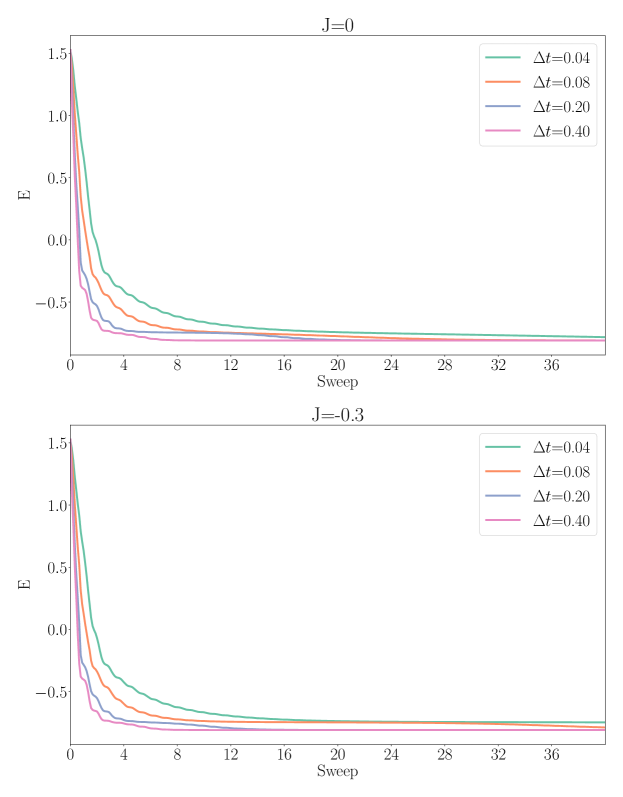
We first analyze the stability of tcDMRG on a 3x3 lattice with =8 and =1, and . We report in Figure 1 the energy convergence of iTD-DMRG and tcDMRG(=-0.3) for varying time steps for the real-space representation with =300. As we will show in the following, this value delivers converged energies. Both iTD-DMRG and tcDMRG converge smoothly, the faster convergence being obtained with the largest time step, of 0.40. For a fixed sweep number, larger time steps corresponds to longer overall propagation times, which enables to reach the limit faster. Note, however, that the computational cost of solving the local differential equation of Eq. (15) increases with the time step because a larger number of iterations is required to converge the iterative approximation of the exponential operator. For =0.40, the Lanczos approximation of the local representation of the imaginary-time propagator converges within 15 iterations in all cases. These results confirm that, unlike TI-DMRG, imaginary-time TD-DMRG can reliably optimize the ground-state wave function of non-Hermitian Hamiltonians.
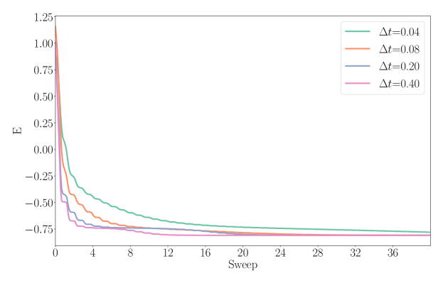
As we show in Figure 2, the same trend is observed for the -space Fermi-Hubbard Hamiltonian. The fastest convergence (12 sweeps) is observed with =0.4 au. With smaller time steps, the energy converges to a local minimum between sweeps 10 and 20, and only afterwards the algorithm converges to the correct limit. For this reason, if not otherwise stated, in the following we set =0.40 for all calculations.
| =0 | =-0.1 | =-0.3 | =-0.5 | TI | ||
|---|---|---|---|---|---|---|
| Real space | 100 | -0.8000 | -0.8006 | -0.7999 | -0.7997 | -0.8000 |
| 200 | -0.8084 | -0.8085 | -0.8084 | -0.8085 | -0.8084 | |
| 300 | -0.8094 | -0.8094 | -0.8094 | -0.8094 | -0.8094 | |
| space | 100 | -0.7537 | -0.7547 | -0.7616 | -0.7760 | -0.7537 |
| 200 | -0.8061 | -0.8060 | -0.8063 | -0.8070 | -0.8061 | |
| 300 | -0.8094 | -0.8094 | -0.8094 | -0.8094 | -0.8094 | |
| space Fiedler | 100 | -0.7608 | -0.7620 | -0.7670 | -0.7770 | -0.7608 |
| 200 | -0.8074 | -0.8074 | -0.8075 | -0.8082 | -0.8074 | |
| 300 | -0.8094 | -0.8094 | -0.8094 | -0.8094 | -0.8094 |
We depict in Table 1 the TI-DMRG, iTD-DMRG, and tcDMRG energy convergence with bond dimension and the transcorrelation parameter for both Hamiltonian representation. As expected, all methods converge towards the reference full-CI energyShi and Zhang (2013) with =300. Note that this value is large for a 9-orbital system, and this is due to the breakdown of the area law for long-ranged Hamiltonians, as we already noted in Section II. As highlighted by Ref. 97, the average interaction range of the Hamiltonian can be strongly reduced by optimizing the orbital sorting in the one-dimensional DMRG lattice based on the so-called Fiedler ordering.Barcza et al. (2011) This orbital sorting minimizes the distance between strongly interacting orbitals, where the interaction strength is evaluated from the mutual informationLegeza and Sólyom (2003); Rissler, Noack, and White (2006) calculated for the MPS optimized with a partially converged MPS, here obtained with TI-DMRG with =100. Note that in Ref. 97 the impact of the ordering on the wave function entanglement is analyzed only qualitatively. Here we assess its effect also on the energy convergence with the bond dimension . As expected, we show in Table 1, the energy for a given value is consistently lower with the Fiedler ordering than with the standard one.
We report in Table 1 tcDMRG results obtained with different values. For the real-space Fermi-Hubbard Hamiltonian, the tcDMRG energy matches the TI-DMRG one for all values for =200 and 300. With =100, the energy difference between TI-DMRG and tcDMRG is smaller than 0.0006 in all cases. The transcorrelated ansatz of Eq. (4) does not produce therefore a more compact MPS when applied to the real-space two-dimensional Fermi-Hubbard Hamiltonian. This agrees with the fact that in Ref. 59 Alavi and co-workers applied the transcorrelated FCIQMC algorithm to the -space two-dimensional Fermi-Hubbard Hamiltonian, and they did not present any results for the real-space representation.
The energy difference between TI-DMRG and tcDMRG is instead considerable for the -space representation. In this case, the difference between the tcDMRG(=-0.5) energies obtained with =100 and =300 is nearly halved compared to the corresponding TI-DMRG data. Note that a correlation factor of =-0.5 is similar to the values optimized in Ref. 59 for lattices with similar values. This confirms that the ground-state wave function of the 3x3 Fermi-Hubbard Hamiltonian can be encoded as a much more compact MPS with the addition of a Gutzwiller correlator.
| =0 | =-0.1 | =-0.3 | =-0.5 | =-0.5 Fiedler | TI | ||
|---|---|---|---|---|---|---|---|
| -space | 500 | -1.0248 | -1.0249 | -1.0255 | -1.0269 | -1.0260 | -1.0249 |
| 1000 | -1.0282 | -1.0281 | -1.0284 | -1.0285 | -1.0283 | -1.0283 | |
| 2000 | -1.0288 | -1.0288 | -1.0288 | -1.0288 | -1.0285 | -1.0288 |
We report in Table 2 the iTD-DMRG and tcDMRG results for a larger, 4x4 lattice with =8, =1, =4, and =4, a parameter set that corresponds to an intermediate correlation regime. The energy convergence with is slower than for the 3x3 lattice, and the TI-DMRG energy matches the reference valueShi and Zhang (2013) with =2000. Also in this case, the energy convergence with is faster for tcDMRG than for iTD-DMRG. The difference between =500 and fully-converged tcDMRG(=-0.5) energies is twice as small than for TI-DMRG. The lowest energy, for a given value, is consistently obtained with tcDMRG(=-0.5) and the Fiedler orbital sorting.
We have applied so-far tcDMRG to either small or weakly-correlated Hamiltonians, for which iTD-DMRG, when combined with an optimized orbital sorting, can converge the energy with reasonable values. The efficiency of tcDMRG becomes apparent in the strong correlation regime, such as for the 4x4 Fermi-Hubbard Hamiltonian with =4, =1, =8, and =8. We report in Table 3 the corresponding TI-DMRG, iTD-DMRG, and tcDMRG energies for varying and values and different orbital sortings. To avoid convergence into local minima, we adopted the so-called density-matrix perturbation theory approach by WhiteWhite (2005) extended to a two-site optimizer for all TI-DMRG simulations. The computational cost of this perturbative scheme is high, especially for large values, and would render tcDMRG calculations unpractical. To avoid a large computational overhead, we adopted the following protocol: we optimized the wave function with TI-DMRG and =500 adding the density-matrix perturbation. Then, we started TI-DMRG optimizations for larger values with the resulting MPS as starting guess. Finally, we ran all tcDMRG calculations for a given values with the MPS optimized with TI-DMRG and the same value as initial guess.
| =-0.1 | =-0.3 | =-0.5 | TI | ||
| -space | 500 | -0.7900 | -0.7779 | -0.8496 | -0.7862 |
| 1000 | -0.8145 | -0.8279 | -0.8536 | -0.8128 | |
| 2000 | -0.8310 | -0.8391 | -0.8528 | -0.8297 | |
| -space Fiedler | 500 | -0.8485 | -0.8495 | -0.8515 | -0.8484 |
| 1000 | -0.8500 | -0.8505 | -0.8513 | -0.8500 | |
| 2000 | -0.8507 | -0.8511 | -0.8514 | -0.8507 | |
| 500 Herm. | -0.8485 | -0.8491 | -0.8496 | -0.8484 |
As expected, the energy convergence of TI-DMRG with is much slower than for the previous Hamiltonian, and the =2000 energy () is still far from being converged to the reference result (-0.8514).Shi and Zhang (2013) The energy convergence of tcDMRG with the bond dimension is, however, much faster. The faster convergence is delivered by tcDMRG(=-0.5) that converges below 0.001 with =2000.
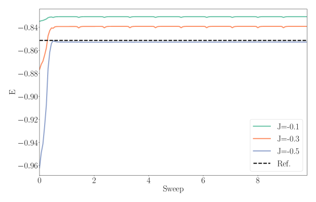
As we show in Figure 3, our computational procedure that starts the tcDMRG imaginary-time propagation from the MPS optimized with TI-DMRG converges the energy efficiently with 2-3 sweeps. It is also worth noting that the energy is lower than the reference, full-CI value for =0.3 and =0.5. We recall that the energy is the expectation value of the transcorrelated Hamiltonian (see Eq. (8)) over the MPS and, as we already highlighted in Section II, the variational principle does not apply. Therefore, an energy lower than the exact, full-CI one is physically acceptable in this case. We highlight that, unlike tcDMRG, a variational-based optimization starting from the TI guess would not converge to the correct minimum. We conclude by noting that the value that provides the best match with the reference data is 0.5. This value agrees with the optimal value obtained in Ref. 59 based on the optimization strategy described in Ref. 67 for a 18-sites Fermi-Hubbard Hamiltonian with the same value. This suggest that the same algorithm,Wahlen-Strothman et al. (2015) that requires the solution of a Coupled Cluster-like equation, can be effectively applied to determine the optimal value for tcDMRG. Note that the results reported in Figure 3 also indicate that the transcorrelation parameter cannot be optimized variationally.
As we show in Table 3, the orbital sorting has a critical impact in the energy convergence of DMRG. With the Fiedler ordering, the TI-DMRG energy obtained with =500 is only 0.0023 higher than the reference energy, while the same difference with the Fiedler ordering is larger than 0.04. However, even by adopting the Fiedler ordering, the energy is not converged even with =2000. By combining the optimized orbital ordering with tcDMRG(=-0.5), the energy differs from the reference one by only 10-4 already with =500. Therefore, the energy convergence of tcDMRG with the bond dimension is in this case truly faster than that of TI-DMRG. This further confirms that, also in the presence of strong correlation, the ground state of the Fermi-Hubbard model can be parametrized as Eq. (4), where can be efficiently represented as a low-entanglement wave function and optimized by applying iTD-DMRG to the transcorrelated Hamiltonian.
Alavi and co-workersDobrautz, Luo, and Alavi (2019) showed that, if, the right lowest-energy eigenvector of the transcorrelated Hamiltonian can be represented as compact CI wave functions, the left one will be represented by a much less compact expansion. Similarly, as we show in the last row of Table 3, the convergence of the energy of the left eigenvector is slower than for the right one (as discussed in Ref. 59, the right-eigenvector corresponding to a given value can be optimized with tcDMRG by setting the Jastrow factor to ).
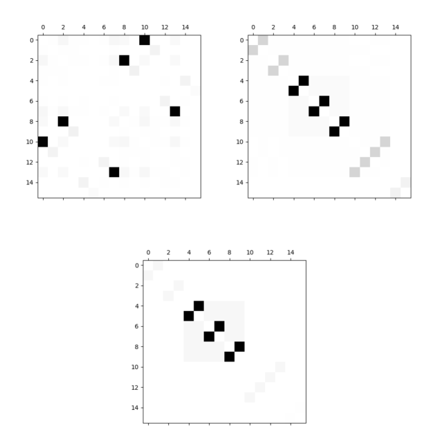
To further characterize the entanglement structure of the ground-state wave function of the transcorrelated Hamiltonian, we report in Figure 4 a graphical representation of the orbital mutual information matrix ,Legeza and Sólyom (2003); Rissler, Noack, and White (2006); Stein and Reiher (2019) with
| (18) |
calculated with TI-DMRG and tcDMRG(=-0.5) for different orbital orderings. is the single-orbital entropy for orbital , defined as
| (19) |
where is the -th eigenvalue of the one-orbital reduced density matrix. Similarly, is the two-orbital entropy, defined as
| (20) |
where the -th eigenvalue of the two-orbital reduced density matrix for orbitals and . As expected, the mutual information matrix has a sparse structure with the standard ordering, while it becomes diagonally dominant for the MPS constructed with the Fiedler ordering. Most importantly, the magnitude of most non-zero elements of the TI-DMRG mutual information matrix are much smaller for tcDMRG(=-0.5). This further confirms that the multi-reference character, measured as orbital entanglement, of the ground state of the transcorrelated Hamiltonian is much smaller than that of the original Fermi-Hubbard Hamiltonian. For this reason, the former can be much more efficiently represented as an MPS. We recall that a similar regularization of the orbital mutual information has been previously observed when combining DMRG with short-range DFT (DMRG-srDFT).Hedegård et al. (2015) In DMRG-srDFT the Hamiltonian is modified to include only the long-range part of the electron-electron Coulomb interaction. Similarly, tcDMRG removes dynamical correlation with the Jastrow factorization of the wave function. In both cases, the mutual information associated to the DMRG wave function becomes more sparse since it is large only for the orbitals coupled by pure static correlation effects.
| Nα | Nβ | TI-DMRG | tcDMRG | Ref. | ||
|---|---|---|---|---|---|---|
| 4 | 12 | 12 | 500 | -1.1500 | -1.1804 | -1.1853 |
| 2 | 18 | 18 | 500 | -1.1345 | -1.1530 | -1.1516 |
| 4 | 18 | 18 | 500 | -0.8206 | -0.8596 | -0.8574 |
| 4 | 18 | 18 | 1000 | -0.8307 | -0.8580 | -0.8574 |
We report in Table 4 the TI-DMRG and tcDMRG energies of the 6x6 Fermi-Hubbard lattice, a system that has been studied with the transcorrelated variant of FCIQMCDobrautz, Luo, and Alavi (2019) and which is out of the reach for exact-diagonalization approaches, for various fillings and ratios. To limit the computational cost, we obtained the tcDMRG results with the single-site imaginary-time propagator starting from the MPS optimized with TI-DMRG. In all cases, we sorted the orbitals in the lattice with the Fiedler ordering obtained with TI-DMRG(=500). Moreover, we set the parameter to the optimal value taken from Ref. 59. The results reported in Table 4 confirm that, also for large lattices, the energy convergence with of tcDMRG is much faster than for standard TI-DMRG. In all cases, the difference between TI-DMRG(=500) and the reference energies is larger than 0.02. The error becomes one order of magnitude smaller with tcDMRG(=500), and is consistently lower than 0.004. By further increasing to 1000, the energy of the half-filled 6x6 lattice with =4, which is the most strongly correlated lattice among the ones studied here, the tcDMRG energy matches the reference one with an error smaller than 10-3.
IV Conclusions
In this work, we introduced transcorrelated DMRG theory that optimizes the ground-state wave function of the transcorrelated Hamiltonian as a matrix product state. The optimization algorithm is tailored to the problem: imaginary-time time-dependent DMRG. Unlike standard time-independent DMRG relying on the variational principle, iTD-DMRG can reliably optimize the ground-state energy of non-Hermitian Hamiltonians. We applied tcDMRG to the two-dimensional Fermi-Hubbard Hamiltonian for different sizes, fillings, and interaction strengths. We demonstrate that, both for weak and strong correlation regimes, the energy convergence of tcDMRG is consistently much faster than that of TI-DMRG. In practice, tcDMRG can converge the energy of Fermi-Hubbard lattices including up to 36 sites, which otherwise would be a challenge for standard DMRG approaches due to the constraints imposed by the area law. Our results agree with recent findings in the framework of FCIQMC by Alavi and co-workers, who showed that the ground-state of the electronicCohen et al. (2019) and Fermi-HubbardDobrautz, Luo, and Alavi (2019) transcorrelated Hamiltonians are efficiently represented by very compact configuration-interaction expansions. In addition, we showed in the present work that the ground-state wave functions belong, more generally, to the class of low-entanglement wave functions and can be therefore encoded as a compact MPS. Note that this conclusion extends the findings of Alavi and co-workersDobrautz, Luo, and Alavi (2019) since a compact MPS wave function can encode both sparse and dense full-CI expansions.
The successful application of the tcDMRG algorithm to the two-dimensional Fermi-Hubbard Hamiltonian suggests that the same theory can be applied as successfully to the electronic Hamiltonian as well.Cohen et al. (2019) In this case, the Jastrow factor in conveniently expressed in real space because the similarity-transformed Hamiltonian includes exactly only up to three-body terms, the main hurdle being the need of calculating the resulting three-centers integrals. However, we expect that tcDMRG will be even more efficient when applied to electronic-structure problems for two reasons. In fact, the Gutzwiller correlator of the transcorrelated Fermi-Hubbard Hamiltonian is governed by a single parameter. Conversely, the real-space Jastrow factor includes a different correlation parameter for each orbital pair. The wave function parametrization is, therefore, much more flexible and can be adapted to the specific molecular system under analysis. Moreover, the three-body potential term appearing in the transcorrelated Fermi-Hubbard Hamiltonian couples any possible combination of six different orbitals. The MPO representation of the resulting Hamiltonian is highly non-compact, even though in the present work we discussed a way to encode it efficiently. For the quantum-chemical case, it will be possible to exploit orbital locality to screen and compress the three-body part of the Hamiltonian and encode it as a compact MPO and to further enhance the tcDMRG efficiency. We showed that the similarity transformation underlying tcDMRG regularizes the wave function entanglement and makes the distinction between strongly- and weakly-correlated orbitals more rigid. This suggests that tcDMRG can be effectively combined with active-space based approaches, where dynamical correlation effects are added a-posteriori with perturbation theory or with multi-reference variants of the Coupled-Cluster method.Li et al. (1997); Kinoshita, Hino, and Bartlett (2005); Veis et al. (2016); Evangelista (2018) All these extensions are currently explored in our laboratory and results will be reported in future work.
Acknowledgements.
This work was supported by ETH Zürich through the ETH Fellowship No. FEL-49 18-1.References
- Booth, Thom, and Alavi (2009) G. H. Booth, A. J. W. Thom, and A. Alavi, “Fermion Monte Carlo without fixed nodes: A game of life, death, and annihilation in Slater determinant space,” J. Chem. Phys. 131, 54106 (2009).
- Cleland, Booth, and Alavi (2010) D. Cleland, G. H. Booth, and A. Alavi, “Communications: Survival of the fittest: Accelerating convergence in full configuration-interaction quantum Monte Carlo,” J. Chem. Phys. 132, 041103 (2010).
- Huron, Malrieu, and Rancurel (1973) B. Huron, J. P. Malrieu, and P. Rancurel, “Iterative perturbation calculations of ground and excited state energies from multiconfigurational zeroth-order wave functions,” J. Chem. Phys. 58, 5745–5759 (1973).
- Evangelisti, Daudey, and Malrieu (1983) S. Evangelisti, J.-P. Daudey, and J.-P. Malrieu, “Convergence of an improved CIPSI algorithm,” Chem. Phys. 75, 91–102 (1983).
- Zhang and Evangelista (2016) T. Zhang and F. A. Evangelista, “A Deterministic Projector Configuration Interaction Approach for the Ground State of Quantum Many-Body Systems,” J. Chem. Theory Comput. 12, 4326–4337 (2016).
- Tubman et al. (2016) N. M. Tubman, J. Lee, T. Y. Takeshita, M. Head-Gordon, and K. B. Whaley, “A deterministic alternative to the full configuration interaction quantum Monte Carlo method,” J. Chem. Phys. 145, 044112 (2016).
- Eriksen, Lipparini, and Gauss (2017) J. J. Eriksen, F. Lipparini, and J. Gauss, “Virtual Orbital Many-Body Expansions: A Possible Route towards the Full Configuration Interaction Limit,” J. Phys. Chem. Lett. 8, 4633–4639 (2017).
- White (1992) S. R. White, “Density matrix formulation for quantum renormalization groups,” Phys. Rev. Lett. 69, 2863–2866 (1992).
- White (1993) S. R. White, “Density-matrix algorithms for quantum renormalization groups,” Phys. Rev. B 48, 10345–10356 (1993).
- Legeza et al. (2008) Ö. Legeza, R. M. Noack, J. Sólyom, and L. Tincani, “Applications of quantum information in the density-matrix renormalization group,” Lect. Notes Phys. 739, 653–664 (2008).
- Chan et al. (2008) G. K.-L. Chan, J. J. Dorando, D. Ghosh, J. Hachmann, E. Neuscamman, H. Wang, and T. Yanai, “An Introduction to the Density Matrix Renormalization Group Ansatz in Quantum Chemistry,” in Frontiers in Quantum Systems in Chemistry and Physics (Springer Netherlands, 2008) pp. 49–65.
- Chan and Zgid (2009) G. K. L. Chan and D. Zgid, “The Density Matrix Renormalization Group in Quantum Chemistry,” Annual Reports in Computational Chemistry 5, 149–162 (2009).
- Marti and Reiher (2010) K. H. Marti and M. Reiher, “The density matrix renormalization group algorithm in quantum chemistry,” Z. Phys. Chem. 224, 583–599 (2010).
- Schollwöck (2011) U. Schollwöck, “The density-matrix renormalization group in the age of matrix product states,” Ann. Phys. 326, 96–192 (2011).
- Chan and Sharma (2011) G. K.-L. Chan and S. Sharma, “The Density Matrix Renormalization Group in Quantum Chemistry,” Annu. Rev. Phys. Chem. 62, 465–481 (2011).
- Wouters and Van Neck (2013) S. Wouters and D. Van Neck, “The density matrix renormalization group for ab initio quantum chemistry,” Eur. Phys. J. D 31, 395–402 (2013).
- Kurashige (2014) Y. Kurashige, “Multireference electron correlation methods with density matrix renormalisation group reference functions,” Mol. Phys. 112, 1485–1494 (2014).
- Olivares-Amaya et al. (2015) R. Olivares-Amaya, W. Hu, N. Nakatani, S. Sharma, J. Yang, and G. K.-L. Chan, “The ab-initio density matrix renormalization group in practice,” J. Chem. Phys. 142, 34102 (2015).
- Szalay et al. (2015) S. Szalay, M. Pfeffer, V. Murg, G. Barcza, F. Verstraete, R. Schneider, and Ö. Legeza, “Tensor product methods and entanglement optimization for ab initio quantum chemistry,” Int. J. Quantum Chem. 115, 1342–1391 (2015).
- Yanai et al. (2015) T. Yanai, Y. Kurashige, W. Mizukami, J. Chalupský, T. N. Lan, and M. Saitow, “Density matrix renormalization group for ab initio calculations and associated dynamic correlation methods: A review of theory and applications,” Int. J. Quantum Chem. 115, 283–299 (2015).
- Knecht et al. (2016) S. Knecht, E. D. Hedegård, S. Keller, A. Kovyrshin, Y. Ma, A. Muolo, C. J. Stein, and M. Reiher, “New Approaches for ab initio Calculations of Molecules with Strong Electron Correlation,” Chimia 70, 244–251 (2016).
- Baiardi and Reiher (2020) A. Baiardi and M. Reiher, “The density matrix renormalization group in chemistry and molecular physics: Recent developments and new challenges,” J. Chem. Phys. 152, 040903 (2020).
- Williams et al. (2020) K. T. Williams, Y. Yao, J. Li, L. Chen, H. Shi, M. Motta, C. Niu, U. Ray, S. Guo, R. J. Anderson, J. Li, L. N. Tran, C.-N. Yeh, B. Mussard, S. Sharma, F. Bruneval, M. van Schilfgaarde, G. H. Booth, G. K.-L. Chan, S. Zhang, E. Gull, D. Zgid, A. Millis, C. J. Umrigar, and L. K. Wagner, “Direct Comparison of Many-Body Methods for Realistic Electronic Hamiltonians,” Phys. Rev. X 10, 011041 (2020).
- Eriksen et al. (2020) J. J. Eriksen, T. A. Anderson, J. E. Deustua, K. Ghanem, D. Hait, M. R. Hoffmann, S. Lee, D. S. Levine, I. Magoulas, J. Shen, N. M. Tubman, K. B. Whaley, E. Xu, Y. Yao, N. Zhang, A. Alavi, G. K.-L. Chan, M. Head-Gordon, W. Liu, P. Piecuch, S. Sharma, S. L. Ten-no, C. J. Umrigar, and J. Gauss, “The Ground State Electronic Energy of Benzene,” J. Phys. Chem. Lett. 11, 8922–8929 (2020).
- Kurashige and Yanai (2011) Y. Kurashige and T. Yanai, “Second-order perturbation theory with a density matrix renormalization group self-consistent field reference function: Theory and application to the study of chromium dimer,” J. Chem. Phys. 135, 94104 (2011).
- Sharma and Chan (2014) S. Sharma and G. K.-L. Chan, “A flexible multi-reference perturbation theory by minimizing the Hylleraas functional with matrix product states,” J. Chem. Phys. 141, 111101 (2014).
- Kurashige et al. (2014) Y. Kurashige, J. Chalupský, T. N. Lan, and T. Yanai, “Complete active space second-order perturbation theory with cumulant approximation for extended active-space wavefunction from density matrix renormalization group,” J. Chem. Phys. 141, 174111 (2014).
- Roemelt, Guo, and Chan (2016) M. Roemelt, S. Guo, and G. K.-L. Chan, “A projected approximation to strongly contracted N-electron valence perturbation theory for DMRG wavefunctions,” J. Chem. Phys. 144, 204113 (2016).
- Ren, Yi, and Shuai (2016) J. Ren, Y. Yi, and Z. Shuai, “Inner Space Perturbation Theory in Matrix Product States: Replacing Expensive Iterative Diagonalization,” J. Chem. Theory Comput. 12, 4871–4878 (2016).
- Wouters, Van Speybroeck, and Van Neck (2016) S. Wouters, V. Van Speybroeck, and D. Van Neck, “DMRG-CASPT2 study of the longitudinal static second hyperpolarizability of all-trans polyenes,” J. Chem. Phys. 145, 54120 (2016).
- Guo et al. (2016) S. Guo, M. A. Watson, W. Hu, Q. Sun, and G. K.-L. Chan, “N -Electron Valence State Perturbation Theory Based on a Density Matrix Renormalization Group Reference Function, with Applications to the Chromium Dimer and a Trimer Model of Poly( p -Phenylenevinylene),” J. Chem. Theory Comput. 12, 1583–1591 (2016).
- Sharma, Jeanmairet, and Alavi (2016) S. Sharma, G. Jeanmairet, and A. Alavi, “Quasi-degenerate perturbation theory using matrix product states,” J. Chem. Phys. 144, 34103 (2016).
- Freitag et al. (2017) L. Freitag, S. Knecht, C. Angeli, and M. Reiher, “Multireference Perturbation Theory with Cholesky Decomposition for the Density Matrix Renormalization Group,” J. Chem. Theory Comput. 13, 451–459 (2017).
- Sharma et al. (2017a) S. Sharma, G. Knizia, S. Guo, and A. Alavi, “Combining Internally Contracted States and Matrix Product States To Perform Multireference Perturbation Theory,” J. Chem. Theory Comput. 13, 488–498 (2017a).
- Guo, Li, and Chan (2018) S. Guo, Z. Li, and G. K.-L. Chan, “Communication: An efficient stochastic algorithm for the perturbative density matrix renormalization group in large active spaces,” J. Chem. Phys. 148, 221104 (2018).
- Sharma et al. (2017b) S. Sharma, A. A. Holmes, G. Jeanmairet, A. Alavi, and C. J. Umrigar, “Semistochastic Heat-Bath Configuration Interaction Method: Selected Configuration Interaction with Semistochastic Perturbation Theory,” J. Chem. Theory Comput. 13, 1595–1604 (2017b).
- Garniron et al. (2017) Y. Garniron, A. Scemama, P. F. Loos, and M. Caffarel, “Hybrid stochastic-deterministic calculation of the second-order perturbative contribution of multireference perturbation theory,” J. Chem. Phys. 147, 034101 (2017).
- Mahajan et al. (2019) A. Mahajan, N. S. Blunt, I. Sabzevari, and S. Sharma, “Multireference configuration interaction and perturbation theory without reduced density matrices,” J. Chem. Phys. 151, 211102 (2019).
- Toulouse, Colonna, and Savin (2004) J. Toulouse, F. Colonna, and A. Savin, “Long-range - Short-range separation of the electron-electron interaction in density-functional theory,” Phys. Rev. A 70, 62505 (2004).
- Li Manni et al. (2014) G. Li Manni, R. K. Carlson, S. Luo, D. Ma, J. Olsen, D. G. Truhlar, and L. Gagliardi, “Multiconfiguration pair-density functional theory,” J. Chem. Theory Comput. 10, 3669–3680 (2014).
- Hedegård et al. (2015) E. D. Hedegård, S. Knecht, J. S. Kielberg, H. J. Aagaard Jensen, and M. Reiher, “Density matrix renormalization group with efficient dynamical electron correlation through range separation,” J. Chem. Phys. 142, 224108 (2015).
- Giner et al. (2018) E. Giner, B. Pradines, A. Ferté, R. Assaraf, A. Savin, and J. Toulouse, “Curing basis-set convergence of wave-function theory using density-functional theory: A systematically improvable approach,” J. Chem. Phys. 149, 194301 (2018).
- Sharma et al. (2019) P. Sharma, V. Bernales, S. Knecht, D. G. Truhlar, and L. Gagliardi, “Density matrix renormalization group pair-density functional theory (DMRG-PDFT): singlet–triplet gaps in polyacenes and polyacetylenes,” Chem. Sci. 10, 1716–1723 (2019).
- Ten-no (2004) S. Ten-no, “Initiation of explicitly correlated Slater-type geminal theory,” Chem. Phys. Lett. 398, 56–61 (2004).
- Klopper et al. (2006) W. Klopper, F. R. Manby, S. Ten-No, and E. F. Valeev, “R12 methods in explicitly correlated molecular electronic structure theory,” Int. Rev. Phys. Chem.. 25, 427–468 (2006).
- Kong, Bischoff, and Valeev (2012) L. Kong, F. A. Bischoff, and E. F. Valeev, “Explicitly correlated R12/F12 methods for electronic structure,” Chem. Rev. 112, 75–107 (2012).
- Hättig et al. (2012) C. Hättig, W. Klopper, A. Köhn, and D. P. Tew, “Explicitly correlated electrons in molecules,” Chem. Rev. 112, 4–74 (2012).
- Hättig, Tew, and Köhn (2010) C. Hättig, D. P. Tew, and A. Köhn, “Communications: Accurate and efficient approximations to explicitly correlated coupled-cluster singles and doubles, CCSD-F12,” J. Chem. Phys. 132, 231102 (2010).
- Ma and Werner (2018) Q. Ma and H.-J. Werner, “Explicitly correlated local coupled-cluster methods using pair natural orbitals,” Wiley Interdiscip. Rev. Comput. Mol. Sci. 8, e1371 (2018).
- Shiozaki and Werner (2010) T. Shiozaki and H. J. Werner, “Communication: Second-order multireference perturbation theory with explicit correlation: CASPT2-F12,” J. Chem. Phys. 133, 141103 (2010).
- Shiozaki and Werner (2013) T. Shiozaki and H. J. Werner, “Multireference explicitly correlated F12 theories,” Mol. Phys. 111, 607–630 (2013).
- Boys and Handy (1969) S. F. Boys and N. C. Handy, “The Determination of Energies and Wavefunctions with Full Electronic Correlation,” Proc. R. Soc. A Math. Phys. Eng. Sci. 310, 43–61 (1969).
- Handy (1973) N. C. Handy, “Towards an understanding of the form of correlated wavefunctions for atoms,” J. Chem. Phys. 58, 279–287 (1973).
- Jastrow (1955) R. Jastrow, “Many-body problem with strong forces,” Phys. Rev. 98, 1479–1484 (1955).
- Yanai and Chan (2006) T. Yanai and G. K.-L. Chan, “Canonical transformation theory for multireference problems,” J. Chem. Phys. 124, 194106 (2006).
- Luo (2011) H. Luo, “Complete optimisation of multi-configuration Jastrow wave functions by variational transcorrelated method,” J. Chem. Phys. 135, 024109 (2011).
- Luo (2010) H. Luo, “Variational transcorrelated method,” J. Chem. Phys. 133, 154109 (2010).
- Luo and Alavi (2018) H. Luo and A. Alavi, “Combining the Transcorrelated Method with Full Configuration Interaction Quantum Monte Carlo: Application to the Homogeneous Electron Gas,” J. Chem. Theory Comput. 14, 1403–1411 (2018).
- Dobrautz, Luo, and Alavi (2019) W. Dobrautz, H. Luo, and A. Alavi, “Compact numerical solutions to the two-dimensional repulsive Hubbard model obtained via nonunitary similarity transformations,” Phys. Rev. B 99, 075119 (2019).
- Cohen et al. (2019) A. J. Cohen, H. Luo, K. Guther, W. Dobrautz, D. P. Tew, and A. Alavi, “Similarity transformation of the electronic Schrödinger equation via Jastrow factorization,” J. Chem. Phys. 151, 061101 (2019).
- Motta et al. (2020) M. Motta, T. P. Gujarati, J. E. Rice, A. Kumar, C. Masteran, J. A. Latone, E. Lee, E. F. Valeev, and T. Y. Takeshita, “Quantum simulation of electronic structure with transcorrelated Hamiltonian: increasing accuracy without extra quantum resources,” ArXiv e-prints , 2006.02488 (2020).
- McArdle and Tew (2020) S. McArdle and D. P. Tew, “Improving the accuracy of quantum computational chemistry using the transcorrelated method,” ArXiv e-prints , 2006.11181 (2020).
- Paeckel et al. (2019) S. Paeckel, T. Köhler, A. Swoboda, S. R. Manmana, U. Schollwöck, and C. Hubig, “Time-evolution methods for matrix-product states,” Ann. Phys. 411, 167998 (2019).
- Lubich, Oseledets, and Vandereycken (2015) C. Lubich, I. Oseledets, and B. Vandereycken, “Time integration of tensor trains,” SIAM J. Numer. Anal. 53, 917 (2015).
- Haegeman et al. (2016) J. Haegeman, C. Lubich, I. Oseledets, B. Vandereycken, and F. Verstraete, “Unifying time evolution and optimization with matrix product states,” Phys. Rev. B 94, 165116 (2016).
- Baiardi and Reiher (2019) A. Baiardi and M. Reiher, “Large-scale quantum-dynamics with matrix product states,” J. Chem. Theory Comput. 15, 3481–3498 (2019).
- Wahlen-Strothman et al. (2015) J. M. Wahlen-Strothman, C. A. Jiménez-Hoyos, T. M. Henderson, and G. E. Scuseria, “Lie algebraic similarity transformed Hamiltonians for lattice model systems,” Phys. Rev. B 91, 041114 (2015), arXiv:1409.2203 .
- Tsuneyuki (2008) S. Tsuneyuki, “Transcorrelated Method: Another Possible Way towards Electronic Structure Calculation of Solids,” Prog. Theor. Phys. Supp. 176, 134–142 (2008).
- Neuscamman et al. (2011) E. Neuscamman, H. Changlani, J. Kinder, and G. K. L. Chan, “Nonstochastic algorithms for Jastrow-Slater and correlator product state wave functions,” Phys. Rev. B 84, 205132 (2011).
- Stoudenmire and White (2012) E. Stoudenmire and S. R. White, “Studying Two-Dimensional Systems with the Density Matrix Renormalization Group,” Ann. Rev. Cond. Matt. Phys. 3, 111–128 (2012).
- Motruk et al. (2016) J. Motruk, M. P. Zaletel, R. S. Mong, and F. Pollmann, “Density matrix renormalization group on a cylinder in mixed real and momentum space,” Phys. Rev. B 93, 155139 (2016), arXiv:1512.03318 .
- Ehlers, White, and Noack (2017) G. Ehlers, S. R. White, and R. M. Noack, “Hybrid-space density matrix renormalization group study of the doped two-dimensional Hubbard model,” Phys. Rev. B 95, 125125 (2017) .
- Hastings (2007) M. B. Hastings, “An area law for one-dimensional quantum systems,” J. Stat. Mech. Theory Exp. 2007, P08024—-P08024 (2007).
- Guifre (2004) V. Guifre, “Efficient simulation of one-dimensional quantum many-body systems,” Phys. Rev. Lett. 93, 40501–40502 (2004).
- Al-Hassanieh et al. (2006) K. A. Al-Hassanieh, A. E. Feiguin, J. A. Riera, C. A. Büsser, and E. Dagotto, “Adaptive time-dependent density-matrix renormalization-group technique for calculating the conductance of strongly correlated nanostructures,” Phys. Rev. B 73, 195304 (2006).
- Ronca et al. (2017) E. Ronca, Z. Li, C. A. Jimenez-Hoyos, and G. K. L. Chan, “Time-Step Targeting Time-Dependent and Dynamical Density Matrix Renormalization Group Algorithms with ab Initio Hamiltonians,” J. Chem. Theory Comput. 13, 5560–5571 (2017).
- Frahm and Pfannkuche (2019) L.-H. Frahm and D. Pfannkuche, “Ultrafast ab-initio Quantum Chemistry Using Matrix Product States,” J. Chem. Theory Comput. 15, 2154–2165 (2019).
- Chan and Van Voorhis (2005) G. K. L. Chan and T. Van Voorhis, “Density-matrix renormalization-group algorithms with nonorthogonal orbitals and non-Hermitian operators, and applications to polyenes,” J. Chem. Phys. 122, 204101 (2005).
- Carlon, Henkel, and Schollwöck (1999) E. Carlon, M. Henkel, and U. Schollwöck, “Density matrix renormalization group and reaction-diffusion processes,” Eur. Phys. J. B 12, 99–114 (1999).
- Helms, Ray, and Chan (2019) P. Helms, U. Ray, and G. K. L. Chan, “Dynamical phase behavior of the single- and multi-lane asymmetric simple exclusion process via matrix product states,” Phys. Rev. E 100, 022101 (2019) .
- Helms and Chan (2020) P. Helms and G. K.-L. Chan, “Dynamical Phase Transitions in a 2D Classical Nonequilibrium Model via 2D Tensor Networks,” Phys. Rev. Lett. 125, 140601 (2020).
- Saad (1992) Y. Saad, “Analysis of Some Krylov Subspace Approximations to the Matrix Exponential Operator,” SIAM J. Numer. Anal. 29, 209–228 (1992).
- Keller et al. (2015) S. Keller, M. Dolfi, M. Troyer, and M. Reiher, “An efficient matrix product operator representation of the quantum chemical Hamiltonian,” J. Chem. Phys 143, 244118 (2015).
- Chan et al. (2016) G. K.-l. Chan, A. Keselman, N. Nakatani, Z. Li, and S. R. White, “Matrix product operators, matrix product states, and ab initio density matrix renormalization group algorithms,” J. Chem. Phys. 145, 014102 (2016).
- Pirvu et al. (2010) B. Pirvu, V. Murg, J. I. Cirac, and F. Verstraete, “Matrix product operator representations,” New J. Phys. 12, 25012 (2010).
- Fröwis, Nebendahl, and Dür (2010) F. Fröwis, V. Nebendahl, and W. Dür, “Tensor operators: Constructions and applications for long-range interaction systems,” Phys. Rev. A 81, 62337 (2010).
- Hubig, McCulloch, and Schollwöck (2017) C. Hubig, I. P. McCulloch, and U. Schollwöck, “Generic construction of efficient matrix product operators,” Phys. Rev. B 95, 35129 (2017).
- Ren et al. (2020) J. Ren, W. Li, T. Jiang, and Z. Shuai, “A general automatic method for optimal construction of matrix product operators using bipartite graph theory,” J. Chem. Phys. 153, 084118 (2020).
- Baiardi et al. (2017) A. Baiardi, C. J. Stein, V. Barone, and M. Reiher, “Vibrational Density Matrix Renormalization Group,” J. Chem. Theory Comput. 13, 3764–3777 (2017).
- Baiardi et al. (2019) A. Baiardi, C. J. Stein, V. Barone, and M. Reiher, “Optimization of highly excited matrix product states with an application to vibrational spectroscopy,” J. Chem. Phys. 150, 094113 (2019).
- White and Martin (1999) S. R. White and R. L. Martin, “Ab initio quantum chemistry using the density matrix renormalization group,” J. Chem. Phys. 110, 4127–4130 (1999).
- Chan and Head-Gordon (2002) G. K.-L. Chan and M. Head-Gordon, “Highly correlated calculations with a polynomial cost algorithm: A study of the density matrix renormalization group,” J. Chem. Phys. 116, 4462–4476 (2002).
- Singh, Pfeifer, and Vidal (2011) S. Singh, R. N. C. Pfeifer, and G. Vidal, “Tensor network states and algorithms in the presence of a global U(1) symmetry,” Phys. Rev. B 83, 115125 (2011).
- Dolfi et al. (2014) M. Dolfi, B. Bauer, S. Keller, A. Kosenkov, T. Ewart, A. Kantian, T. Giamarchi, and M. Troyer, “Matrix product state applications for the ALPS project,” Comput. Phys. Commun. 185, 3430–3440 (2014).
- Kantian et al. (2019) A. Kantian, M. Dolfi, M. Troyer, and T. Giamarchi, “Understanding repulsively mediated superconductivity of correlated electrons via massively parallel density matrix renormalization group,” Phys. Rev. B 100, 75138 (2019).
- Brabec et al. (2020) J. Brabec, J. Brandejs, K. Kowalski, S. Xantheas, Ö. Legeza, and L. Veis, “Massively parallel quantum chemical density matrix renormalization group method,” ArXiv e-prints , 2001.04890 (2020) .
- Ehlers et al. (2015) G. Ehlers, J. Sólyom, O. Legeza, and R. M. Noack, “Entanglement structure of the Hubbard model in momentum space,” Phys. Rev. B 92, 235116 (2015).
- Shi and Zhang (2013) H. Shi and S. Zhang, “Symmetry in auxiliary-field quantum Monte Carlo calculations,” Phys. Rev. B 88, 125132 (2013).
- Barcza et al. (2011) G. Barcza, Ö. Legeza, K. H. Marti, and M. Reiher, “Quantum-information analysis of electronic states of different molecular structures,” Phys. Rev. A 83, 012508 (2011).
- Legeza and Sólyom (2003) Ö. Legeza and J. Sólyom, “Optimizing the density-matrix renormalization group method using quantum information entropy,” Phys. Rev. B 68, 195116 (2003).
- Rissler, Noack, and White (2006) J. Rissler, R. M. Noack, and S. R. White, “Measuring orbital interaction using quantum information theory,” Chem. Phys. 323, 519–531 (2006).
- White (2005) S. R. White, “Density matrix renormalization group algorithms with a single center site,” Phys. Rev. B 72, 180403 (2005).
- Stein and Reiher (2019) C. J. Stein and M. Reiher, “autoCAS: A Program for Fully Automated Multiconfigurational Calculations,” J. Comput. Chem. 40, 2216 (2019).
- Qin, Shi, and Zhang (2016) M. Qin, H. Shi, and S. Zhang, “Benchmark study of the two-dimensional Hubbard model with auxiliary-field quantum Monte Carlo method,” Phys. Rev. B 94, 085103 (2016).
- Li et al. (1997) X. Li, G. Peris, J. Planelles, F. Rajadall, and J. Paldus, “Externally corrected singles and doubles coupled cluster methods for open-shell systems,” J. Chem. Phys. 107, 90–98 (1997).
- Kinoshita, Hino, and Bartlett (2005) T. Kinoshita, O. Hino, and R. J. Bartlett, “Coupled-cluster method tailored by configuration interaction,” J. Chem. Phys. 123, 074106 (2005).
- Veis et al. (2016) L. Veis, A. Antalík, J. Brabec, F. Neese, Ö. Legeza, and J. Pittner, “Coupled Cluster Method with Single and Double Excitations Tailored by Matrix Product State Wave Functions,” J. Phys. Chem. Lett. 7, 4072–4078 (2016).
- Evangelista (2018) F. A. Evangelista, “Perspective : Multireference coupled cluster theories of dynamical electron correlation,” J. Chem. Phys. 149, 030901 (2018).