1 Introduction

Consider the problem of estimating a degree $d$, real-valued tensor $\theta^{*}\in^{n_{1}\times\cdots\times n_{d}}$, whose entries are observed with noise. As in many problems in high-dimensional statistics, this tensor estimation problem requires a prohibitively large number of observations to solve without the imposition of further structure, and consequently, many structural constraints have been placed in particular applications of tensor estimation. For instance, low “rank” structure is common in chemistry and neuroscience applications (Andersen and Bro, 2003; Möcks, 1988), blockwise constant structure is common in applications to clustering and classification of relational data (Zhou et al., 2007), sparsity is commonly used in data mining applications (Kolda et al., 2005), and variants and combinations of such assumptions have also appeared in other contexts (Zhou et al., 2015). In this paper, we study a flexible, nonparametric structural assumption that generalizes parametric assumptions in applications of tensor models to discrete choice data.

Suppose we are interested in modeling ordinal data, which arises in applications ranging from information retrieval (Dwork et al., 2001) and assortment optimization (Kök et al., 2015) to recommender systems (Baltrunas et al., 2010) and crowdsourcing (Chen et al., 2013); in a generic such problem, we have $n_{1}$ “items”, subsets of which are evaluated using a multiway comparison. In particular, each datum takes the form of a tuple containing $d$ of these items, and a single item that is chosen from the tuple as the “winner” of this comparison. Such data can be represented using a stochastic model of choice: For each tuple $A$ and each item $i\in A$, suppose that $i$ wins the comparison with probability $p(i,A)$. The winner of each comparison is then modeled as a random variable; equivalently, the overall statistical model is described by a $d$-dimensional mean tensor $\theta^{*}\in^{n_{1}\times\cdots\times n_{1}}$, where $\theta^{*}(i_{1},\ldots,i_{d})=p(i_{1},(i_{1},\ldots,i_{d}))$, and our data consist of noisy observations of entries of this tensor. Imposing sensible constraints on the tensor $\theta^{*}$ in these applications goes back to classical, axiomatic work on the subject due to Luce (1959) and Plackett (1975). A natural and flexible assumption is given by simple scalability (Krantz, 1965; McFadden, 1981; Tversky, 1972): this states that each of the $n_{1}$ items can be associated with some scalar utility (item $i$ with utility $u_{i}$), and that the comparison probability is given by

$$\theta^{*}(i_{1},\ldots,i_{d})=f(u_{i_{1}},\ldots,u_{i_{d}}),$$ (1)

where $f$ is a non-decreasing function of its first argument and a coordinate-wise non-increasing function of the remaining arguments. Operationally, an item should not have a lower chance of being chosen as a winner if—all else remaining equal—its utility were to be increased.

There are many models that satisfy the nonparametric simple scalability assumption, in particular, parametric assumptions in which a specific form of the function $f$ is posited. The simplest parameterization is given by $f(u_{1},\ldots,u_{d})=u_{1}/\sum_{j=1}^{d}u_{j}$, which dates back to Luce (1959). A logarithmic transformation of Luce’s parameterization leads to the multinomial logit (MNL) model, which has seen tremendous popularity in applications ranging from transportation (Ben-Akiva et al., 1985) to marketing (Chandukala et al., 2008). See, e.g., McFadden (1974) for a classical but comprehensive introduction to this class of models. However the parametric assumptions of the MNL model have been called into question by a line of work showing that greater flexibility in modeling can lead to improved results in many applications (see, e.g., Farias et al. (2013) and references therein).

The simple scalability (SS) assumption has also been extensively explored when $d=2$, i.e., in the pairwise comparison case. In this case, the nonparametric SS assumption is equivalent to strong stochastic transitivity, and a long line of work (Marschak and Davidson, 1957; McLaughlin and Luce, 1965; Fishburn, 1973) has studied its empirical properties. In particular, the parametric MNL model specialized to this case corresponds to the popular Bradley–Terry–Luce model (Bradley and Terry, 1952; Luce, 1959), and nonparametric models are known to be significantly more robust to misspecification than their parametric counterparts in common applications (Marschak and Davidson, 1957; Ballinger and Wilcox, 1997).

Let us return now to the SS assumption in the general case, and state an equivalent formulation in terms of structure on the tensor $\theta^{*}$. For two vectors of equal dimension, let $x\preceq y$ denote that $x-y\leq 0$ entrywise, and let $\pi$ denote any permutation of $[n_{1}]$ that orders the utilities in the sense that $u_{\pi(1)}\leq\cdots\leq u_{\pi(n_{1})}$. The monotonicity of the function $f$ in the SS assumption (1) ensures that whenever $(i_{1},\ldots,i_{d})\preceq(i_{1}^{\prime},\ldots,i_{d}^{\prime})$, we have

$$\theta^{*}\bigl{(}\pi(i_{1}),\pi^{-1}(i_{2}),\ldots,\pi^{-1}(i_{d})\bigr{)} =f\bigl{(}u_{\pi(i_{1})},u_{\pi^{-1}(i_{2})},\ldots,u_{\pi^{-1}(i_{d})}\bigr{)}$$

$$\leq f\bigl{(}u_{\pi(i^{\prime}_{1})},u_{\pi^{-1}(i^{\prime}_{2})},\ldots,u_{\pi^{-1}(i^{\prime}_{d})}\bigr{)}$$

$$=\theta^{*}\bigl{(}\pi(i^{\prime}_{1}),\pi^{-1}(i_{2}^{\prime}),\ldots,\pi^{-1}(i^{\prime}_{d})\bigr{)}.$$ (2)

Crucially, since the utilities themselves are latent, the permutation $\pi$ is unknown—indeed, it represents the ranking that must be estimated from our data—and so $\theta^{*}$ is a coordinate-wise isotonic tensor with unknown permutations. In the multiway comparison problem, this tensor represents the stochastic model underlying our data, and accurate knowledge of these probabilities is useful, for instance, in informing pricing and revenue management decisions in assortment optimization applications (Kök et al., 2015).

While multiway comparisons form our primary motivation, the flexibility afforded by nonparametric models with latent permutations has also been noticed and exploited in other applications. For instance, in psychometric item-response theory, the Mokken model—which corresponds to imposing structure of the form (1) when $d=2$—is known to be significantly more robust to misspecification that the parametric Rasch model; see van Schuur (2003) for an introduction and survey. In crowd-labeling, the permutation-based model (Shah et al., 2021) has seen empirical success in applications where the parametric Dawid–Skene model (Dawid and Skene, 1979) imposes stringent assumptions. Besides these, there are also several other examples of tensor estimation problems in which parametric structure is frequently assumed; for example, in click modeling (Craswell et al., 2008) and random hypergraph models (Ghoshdastidar and Dukkipati, 2017; Angelini et al., 2015). Similarly to before, nonparametric structure has the potential to generalize and lend flexibility to these parametric models.

It is worth noting that in many of the aforementioned applications, the underlying objects can be clustered into near identical sets. For example, there is evidence that such “indifference sets” of items exist in crowdsourcing (see Shah et al. (2019a, Figure 1) for an illuminating example) and peer review applications involving comparison data (Nguyen et al., 2014); clustering is often used in the application of psychometric evaluation methods (Hardouin and Mesbah, 2004), and many models for communities in hypergraphs posit the existence of such clusters of nodes (Abbe and Montanari, 2013; Ghoshdastidar and Dukkipati, 2017). For a precise mathematical definition of indifference sets and how they induce further structure in the tensor $\theta^{*}$, see Section 2. Whenever such additional structure exists, it is conceivable that estimation can be performed in a more sample-efficient manner; we will precisely quantify such a phenomenon in our exposition in Section 3.

Using these applications as motivation, our goal in this paper is to study the tensor estimation problem under the nonparametric structural assumptions (1) of monotonicity constraints and unknown permutations.

1.1 Related work

Regression problems with unknown permutations were classically studied in applications to record-linkage (DeGroot and Goel, 1980), and similar models have witnessed recent interest driven by other modern applications in machine learning and signal processing; see, e.g., Collier and Dalalyan (2016); Unnikrishnan et al. (2018); Pananjady et al. (2017a, b); Hsu et al. (2017); Abid and Zou (2018); Behr and Munk (2017) for theoretical results and applications. We focus our discussion on the sub-class of such problems involving monotonic shape-constraints and (vector/matrix/tensor) estimation. When $d=1$, the assumption (1) corresponds to the “uncoupled” or “shuffled” univariate isotonic regression problem (Carpentier and Schlueter, 2016). Here, an estimator based on Wasserstein deconvolution is known to attain the minimax rate $\log\log n/\log n$ in (normalized) squared $\ell_{2}$-error for estimation of the underlying (sorted) vector of length $n$ (Rigollet and Weed, 2019). In a recent paper, Balabdaoui et al. (2020) considered a closely related problem, with a focus on isolating the effect of the noise distribution on the deconvolution procedure. A multivariate version of this problem (estimating multiple isotonic functions under a common unknown permutation of coordinates) has also been studied under the moniker of “statistical seriation”, and has been shown to have applications to archaeology and metagenomics (Flammarion et al., 2019; Ma et al., 2021+).

The case $d=2$ has also seen a long line of work in the mathematical statistics community in the context of estimation from pairwise comparisons, wherein the monotonicity assumption (1) corresponds to strong stochastic transitivity, or SST for short (e.g., Chatterjee, 2015; Shah et al., 2017; Chatterjee and Mukherjee, 2019; Shah et al., 2019a; Mao et al., 2020). Relatives of this model have also appeared in the context of prediction in graphon estimation (Chan and Airoldi, 2014; Airoldi et al., 2013) and calibration in crowd-labeling (Shah et al., 2021; Mao et al., 2020). The minimax rate (in normalized, squared Frobenius error) of estimating an $(n^{1/2}\times n^{1/2})$ SST matrix is known to be of the order $n^{-1/2}$ up to a polylogarithmic factor, but many computationally efficient algorithms (Chatterjee, 2015; Shah et al., 2017; Chatterjee and Mukherjee, 2019; Shah et al., 2019a) achieved only the rate $n^{-1/4}$. Recent progress has shown more sophisticated (but still efficient) procedures with improved rates: an algorithm with rate $n^{-3/8}$ was given by Mao et al. (2018), and in recent work, Liu and Moitra (2020) show that a rate $n^{-5/12}$ can be achieved. However, it is still not known whether the minimax rate is attainable by an efficient algorithm. The case of estimating rectangular matrices has also been studied, and the fundamental limits are known to be sensitive to the aspect ratio of the problem (Mao et al., 2020). Interesting adaptation properties are also known in this case, both to parametric structure (Chatterjee and Mukherjee, 2019), and to indifference sets (Shah et al., 2019a).

To the best of our knowledge, analogs of these results have not been explored in the multivariate setting $d\geq 3$, although a significant body of literature has studied parametric models for choice data in this case (see, e.g., Negahban et al. (2018) and references therein).

1.2 Overview of contributions

We begin by considering the minimax risk of estimating bounded tensors satisfying assumption (1), and show in Proposition 1 that when $d\geq 2$, it is dominated by the risk of estimating the underlying ordered coordinate-wise isotonic tensor. In other words, the latent permutations do not significantly influence the statistical difficulty of the problem. We also study the fundamental limits of estimating tensors having indifference set structure, and this allows us to assess the ability of an estimator to adapt to such structure via its adaptivity index (to be defined precisely in equation (3)). We establish two surprising phenomena in this context: First, we show in Proposition 3 that the fundamental limits of estimating these objects preclude a parametric rate, in sharp contrast to the case without unknown permutations. Second, we prove in Theorem 1 that the adaptivity index exhibits a statistical-computational gap under the assumption of a widely-believed conjecture in average-case complexity. In particular, we show that the adaptivity index of any polynomial time computable estimator must grow at least polynomially in $n$, assuming the hypergraph planted clique conjecture (Brennan and Bresler, 2020). Our results also have interesting consequences for the isotonic regression problem without unknown permutations (see Proposition 2 and Corollary 1).

Having established these fundamental limits, we then turn to our main methodological contribution. We propose and analyze—in Theorem 2—an estimator based on Mirsky’s partitioning algorithm (Mirsky, 1971) that estimates the underlying tensor (a) at the minimax rate (up to poly-logarithmic factors) for each $d\geq 3$ whenever this tensor has bounded entries, and (b) with the best possible adaptivity index for polynomial time procedures for all $d\geq 2$. The first of these findings is particularly surprising because it shows that the case $d\geq 3$ of this problem is distinctly different from the bivariate case, in that the minimax risk is achievable with a computationally efficient algorithm. This is in spite of the fact that there are more permutations to estimate as the dimension increases, which, at least in principle, ought to make the problem more difficult both statistically and computationally.

In addition to its favorable risk properties, the Mirsky partition estimator also has several other advantages: it is computable in time sub-quadratic in the size of the input, and its computational complexity also adapts to underlying indifference set structure. In particular, when there are a fixed number of indifference sets, the estimator has almost linear computational complexity with high probability. When specialized to $d=2$, this estimator exhibits significantly better adaptation properties to indifference set structure than known estimators that were designed specifically for this purpose; see Section 3.5 and Appendix A of for statements and discussions of these results.

To complement our upper bounds on the Mirsky partition estimator, we also show, somewhat surprisingly, that many other estimators proposed in the literature (Chatterjee and Mukherjee, 2019; Shah et al., 2019a, 2017), and natural variants thereof, suffer from an extremely large adaptivity index. In particular, they are unable to attain the polynomial time optimal adaptivity index (given by the fundamental limit established by Theorem 1) for any $d\geq 4$. This is in spite of the fact that some of these estimators are minimax optimal for estimation over the class of bounded tensors (see Propositions 4 and 2) for all $d\geq 3$. Thus, we see that simultaneously achieving good worst-case risk properties while remaining computationally efficient and adaptive to structure is a challenging requirement, thereby providing further evidence of the value of the Mirsky partitioning estimator.

1.3 Organization

The rest of this paper is organized as follows. In Section 2, we introduce formally the estimation problem at hand. Section 3 contains full statements and discussions of our main results, and Section 5 contains some concluding remarks. Proofs of the main results are in Section 4. The appendices also contain results that may be of independent interest. In particular, some of our results on adaptation in the special cases $d=2,3$ are postponed to Appendix A, and Appendix B collects some properties of the vanilla isotonic regression estimator.

2 Background and problem formulation

Let $\mathfrak{S}_{k}$ denote the set of all permutations on the set $[k]:\,=\{1,\ldots,k\}$. We interpret ${}^{n_{1}\times\cdots\times n_{d}}$ as the set of all real-valued, tensors of dimension $n_{1}\times\cdots\times n_{d}$. For a set of positive integers $i_{j}\in[n_{j}],j\in[d]$, we use $T(i_{1},\ldots,i_{d})$ to index entry $i_{1},\ldots,i_{d}$ of a tensor $T\in^{n_{1}\times\cdots\times n_{d}}$.

The set of all real-valued, coordinate-wise isotonic functions on the set $[0,1]^{d}$ is denoted by

$$\mathcal{F}_{d}:\,=\left\{f:[0,1]^{d}\to:f(x_{1},x_{2},\ldots,x_{d})\leq f(x^{\prime}_{1},x^{\prime}_{2},\ldots,x^{\prime}_{d})\;\text{when}\;x_{j}\leq x^{\prime}_{j}\;\text{ for }\;j\in[d]\right\}.$$

Let $n_{j}$ denote the number of observations along dimension $j$, with the total number of observations given by $n:\,=\prod_{j=1}^{d}n_{j}$. For $n_{1},\ldots,n_{d}\in\mathbb{N}$, let $\mathbb{L}_{d,n_{1},\ldots,n_{d}}:\,=\prod_{j=1}^{d}[n_{j}]$ denote the $d$-dimensional lattice. With this notation, we assume access to a tensor of observations $Y\in\mathbb{R}^{n_{1}\times\cdots\times n_{d}}$, where

$$Y(i_{1},\ldots,i_{d})=f^{*}\left(\frac{\pi^{*}_{1}(i_{1})}{n_{1}},\frac{\pi^{*}_{2}(i_{2})}{n_{2}},\ldots,\frac{\pi^{*}_{d}(i_{d})}{n_{d}}\right)+\epsilon(i_{1},\ldots,i_{d})\text{ for each }i_{j}\in[n_{j}],\;j\in[d].$$

Here, the function $f^{*}\in\mathcal{F}_{d}$ is unknown, and for each $j\in[d]$, we also have an unknown permutation $\pi^{*}_{j}\in\mathfrak{S}_{n_{j}}$. The tensor $\epsilon\in^{n_{1}\times\cdots\times n_{d}}$ represents noise in the observation process, and we assume that its entries are given by independent standard normal random variables. Denote the noiseless observations on the lattice by

$$\theta^{*}(i_{1},\ldots,i_{d}):\,=f^{*}\left(\frac{\pi^{*}_{1}(i_{1})}{n_{1}},\frac{\pi^{*}_{2}(i_{2})}{n_{2}},\ldots,\frac{\pi^{*}_{d}(i_{d})}{n_{d}}\right)\quad\text{ for each }i_{j}\in[n_{j}],\;j\in[d];$$

this is a generalization of the nonparametric structure that was posited in equation (1).

It is also convenient to define the set of tensors that can be formed by permuting evaluations of a coordinate-wise monotone function on the lattice by the permutations $(\pi_{1},\ldots,\pi_{d})$. Denote this set by

$$\mathcal{M}(\mathbb{L}_{d,n_{1},\ldots,n_{d}};\pi_{1},\ldots,\pi_{d}) :\,=\biggl{\{}\theta\in^{n_{1}\times\cdots\times n_{d}}:\;\exists f\in\mathcal{F}_{d}\;\text{such that }\forall i_{j}\in[n_{j}],\;j\in[d],$$

$$\;\;\quad\qquad\qquad\qquad\theta(i_{1},\ldots,i_{d})=f\left(\frac{\pi_{1}(i_{1})}{n_{1}},\ldots,\frac{\pi_{d}(i_{d})}{n_{d}}\right)\biggl{\}}.$$

We use the shorthand $\mathcal{M}(\mathbb{L}_{d,n_{1},\ldots,n_{d}})$ to denote this set when the permutations are all the identity. Also define the set

$$\mathcal{M}_{{\sf perm}}(\mathbb{L}_{d,n_{1},\ldots,n_{d}}):\,=\bigcup_{\pi_{1}\in\mathfrak{S}_{n_{1}}}\cdots\bigcup_{\pi_{d}\in\mathfrak{S}_{n_{d}}}\mathcal{M}(\mathbb{L}_{d,n_{1},\ldots,n_{d}};\pi_{1},\ldots,\pi_{d})$$

of tensors that can be formed by permuting evaluations of any coordinate-wise monotone function.

For a collection of permutations $\{\pi_{j}\in\mathfrak{S}_{n_{j}}\}_{j=1}^{d}$ and a tensor $T\in^{n_{1}\times\cdots\times n_{d}}$, we let $T\{\pi_{1},\ldots,\pi_{d}\}$ denote the tensor $T$ viewed along permutation $\pi_{j}$ on dimension $j$. Specifically, we have

$$T\{\pi_{1},\ldots,\pi_{d}\}(i_{1},\ldots,i_{d})=T(\pi_{1}(i_{1}),\ldots,\pi_{d}(i_{d}))\quad\text{ for each }\quad i_{j}\in[n_{j}],\;\;j\in[d].$$

With this notation, note the inclusion $\theta^{*}\{(\pi^{*}_{1})^{-1},\ldots,(\pi^{*}_{d})^{-1}\}\in\mathcal{M}(\mathbb{L}_{d,n_{1},\ldots,n_{d}})$. However, since we do not know the permutations $\pi^{*}_{1},\ldots,\pi^{*}_{d}$ a priori, we may only assume that $\theta^{*}\in\mathcal{M}_{{\sf perm}}(\mathbb{L}_{d,n_{1},\ldots,n_{d}})$, and our goal is to denoise our observations and produce an estimate of $\theta^{*}$. We study the empirical $L_{2}$ risk of any such estimate $\widehat{\theta}\in\mathbb{R}^{n_{1}\times\cdots\times n_{d}}$, given by

$$\mathcal{R}_{n}(\widehat{\theta},\theta^{*}) :\,={\mathbb{E}}\left[\ell_{n}^{2}(\widehat{\theta},\theta^{*})\right],\;\text{ where }$$

$$\ell_{n}^{2}(\theta_{1},\theta_{2}) :\,=\frac{1}{n}\sum_{j=1}^{d}\sum_{i_{j}=1}^{n_{j}}\left(\theta_{1}(i_{1},\ldots,i_{d})-\theta_{2}(i_{1},\ldots,i_{d})\right)^{2}.$$

Note that the expectation is taken over both the noise $\epsilon$ and any randomness used to compute the estimate $\widehat{\theta}$. In the case where $\widehat{\theta}\in\mathcal{M}_{{\sf perm}}(\mathbb{L}_{d,n_{1},\ldots,n_{d}})$, we also produce a function estimate $\widehat{f}\in\mathcal{F}_{d}$ and permutation estimates $\widehat{\pi}_{j}\in\mathfrak{S}_{n_{j}}$ for $j\in[d]$, with

$$\widehat{\theta}(i_{1},\ldots,i_{d}):\,=\widehat{f}\left(\frac{\widehat{\pi}_{1}(i_{1})}{n_{1}},\frac{\widehat{\pi}_{2}(i_{2})}{n_{2}},\ldots,\frac{\widehat{\pi}_{d}(i_{d})}{n_{d}}\right)\quad\text{ for each }i_{j}\in[n_{j}],\;j\in[d].$$

Note that in general, the resulting estimates $\widehat{f},\widehat{\pi}_{1},\ldots,\widehat{\pi}_{d}$ need not be unique, but this identifiability issue will not concern us since we are only interested in the tensor $\widehat{\theta}$ as an estimate of the tensor $\theta^{*}$.

As alluded to in the introduction, it is common in multiway comparisons for there to be indifference sets of items that all behave identically. These sets are easiest to describe in the space of functions. For each $j\in[d]$ and $s_{j}\in[n_{j}]$, let $I^{j}_{1},\ldots,I^{j}_{s_{j}}$ denote a set of $s_{j}$ disjoint intervals such that $[0,1]=\cup_{\ell=1}^{s_{j}}I^{j}_{\ell}$. Suppose that for each $\ell$, the length of the interval $I^{j}_{\ell}$ exceeds $1/n_{j}$, so that we are assured that the intersection of $I^{j}_{\ell}$ with the set $\frac{1}{n_{j}}\{1,\ldots,n_{j}\}$ is non-empty. With a slight abuse of terminology, we also refer to this intersection as an interval, and let the tuple $\mathbf{k}^{j}=(k^{j}_{1},\ldots,k^{j}_{s_{j}})$ denote the cardinalities of these intervals, with $\sum_{\ell=1}^{s_{j}}k^{j}_{\ell}=n_{j}$. Let $\mathbf{K}_{s_{j}}$ denote the set of all such tuples, and define $k^{j}_{\max}:\,=\max_{\ell\in[s_{j}]}\mathbf{k}^{j}_{\ell}$. Collect $\{\mathbf{k}^{j}\}_{j=1}^{d}$ in a tuple $\mathbbm{k}=(\mathbf{k}^{1},\ldots,\mathbf{k}^{d})$, and the $d$ values $\{s_{j}\}_{j=1}^{d}$ in a tuple $\mathbf{s}=(s_{1},\ldots,s_{d})$. Let $\mathbb{K}_{\mathbf{s}}$ denote the set of all such tuples $\mathbbm{k}$, and note that the possible values of $\mathbf{s}$ range over the lattice $\mathbb{L}_{d,n_{1},\ldots,n_{d}}$. Finally, let $k^{*}:\,=\min_{j\in[d]}k^{j}_{\max}$. See Figure 1 for an illustration when $d=2$.

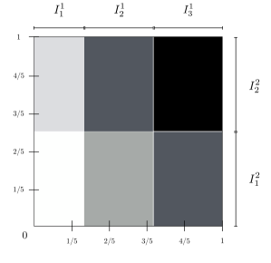
Figure 1: An illustration of a block-wise constant isotonic function on $[0,1]^{2}$, with lighter colors indicating smaller values. We observe this function on a $5\times 5$, equally spaced grid (i.e., $n_{1}=5$). The number of indifference sets along the two dimensions satisfies $s_{1}=3$ and $s_{2}=2$, and their size tuples satisfy $\mathbf{k}^{1}=(1,2,2)$ and $\mathbf{k}^{2}=(2,3)$. As a result, we have $k^{*}=2$.

.

If, for each $j\in[d]$, dimension $j$ of the domain is partitioned into the intervals $I^{j}_{1},\ldots,I^{j}_{s_{j}}$, then the set $[0,1]^{d}$ is partitioned into $s:\,=\prod_{j=1}^{d}s_{j}$ hyper-rectangles. Here, the hyper-rectangular partition is a Cartesian product of univariate partitions, i.e., each hyper-rectangle takes the form $\prod_{j=1}^{d}I^{j}_{\ell_{j}}$ for some sequence of indices $\ell_{j}\in[s_{j}],j\in[d]$. We refer to the intersection of a hyper-rectangle with the lattice $\mathbb{L}_{d,n_{1},\ldots,n_{d}}$ also as a hyper-rectangle, and note that $\mathbbm{k}$ fully specifies such a hyper-rectangular partition. Denote by $\mathcal{M}^{\mathbbm{k},\mathbf{s}}(\mathbb{L}_{d,n_{1},\ldots,n_{d}})$ the set of all $\theta\in\mathcal{M}(\mathbb{L}_{d,n_{1},\ldots,n_{d}})$ that are piecewise constant on a hyper-rectangular partition specified by $\mathbbm{k}$—we have chosen to be explicit about the tuple $\mathbf{s}$ in our notation for clarity. Let $\mathcal{M}^{\mathbbm{k},\mathbf{s}}_{{\sf perm}}(\mathbb{L}_{d,n_{1},\ldots,n_{d}})$ denote the set of all coordinate-wise permuted versions of $\theta\in\mathcal{M}^{\mathbbm{k},\mathbf{s}}(\mathbb{L}_{d,n_{1},\ldots,n_{d}})$.

For the rest of this paper, we operate in the uniform, or balanced case $2\leq n_{1}=\cdots=n_{d}=n^{1/d}$, which is motivated by the comparison setting introduced in Section 1. We use the shorthand $\mathbb{L}_{d,n}$ to represent the uniform lattice and $\mathbb{R}_{d,n}$ to represent balanced tensors. We continue to use the notation $n_{j}$ in some contexts since this simplifies our exposition, and also continue to accommodate distinct permutations $\pi^{*}_{1},\ldots,\pi^{*}_{d}$ and cardinalities of indifference sets $s_{1},\ldots,s_{d}$ along the different dimensions for flexibility.

Let $\widehat{\Theta}$ denote the set of all estimators of $\theta^{*}$, i.e. the set of all measurable functions (of the observation tensor $Y$) taking values in _d,n. Denote the minimax risk over the class of tensors in the set $\mathcal{M}^{\mathbbm{k},\mathbf{s}}_{{\sf perm}}(\mathbb{L}_{d,n})$ by

$$\mathfrak{M}_{d,n}(\mathbbm{k},\mathbf{s}):\,=\inf_{\widehat{\theta}\in\widehat{\Theta}}\;\sup_{\theta^{*}\in\mathcal{M}^{\mathbbm{k},\mathbf{s}}_{{\sf perm}}(\mathbb{L}_{d,n})}\;\mathcal{R}_{n}(\widehat{\theta},\theta^{*}).$$

Note that $\mathfrak{M}_{d,n}(\mathbbm{k},\mathbf{s})$ measures the smallest possible risk achievable with a priori knowledge of the inclusion $\theta^{*}\in\mathcal{M}^{\mathbbm{k},\mathbf{s}}_{{\sf perm}}(\mathbb{L}_{d,n})$. On the other hand, we are interested in estimators that adapt to hyper-rectangular structure without knowing of its existence in advance. One way to measure the extent of adaptation of an estimator $\widehat{\theta}$ is in terms of its adaptivity index to indifference set sizes $\mathbbm{k}$, defined as

$$\mathfrak{A}^{\mathbbm{k},\mathbf{s}}(\widehat{\theta}):\,=\frac{\sup_{\theta^{*}\in\mathcal{M}^{\mathbbm{k},\mathbf{s}}_{{\sf perm}}(\mathbb{L}_{d,n})}\;\mathcal{R}_{n}(\widehat{\theta},\theta^{*})}{\mathfrak{M}_{d,n}(\mathbbm{k},\mathbf{s})}.$$

A large value of this index indicates that the estimator $\widehat{\theta}$ is unable to adapt satisfactorily to the set $\mathcal{M}^{\mathbbm{k},\mathbf{s}}_{{\sf perm}}(\mathbb{L}_{d,n})$, since a much lower risk is achievable when the inclusion $\theta^{*}\in\mathcal{M}^{\mathbbm{k},\mathbf{s}}_{{\sf perm}}(\mathbb{L}_{d,n})$ is known in advance. The global adaptivity index of $\widehat{\theta}$ is then given by

$$\mathfrak{A}(\widehat{\theta}):\,=\max_{\mathbf{s}\in\mathbb{L}_{d,n}}\max_{\mathbbm{k}\in\mathbb{K}_{\mathbf{s}}}\;\mathfrak{A}^{\mathbbm{k},\mathbf{s}}(\widehat{\theta}).$$ (3)

We note that similar definitions of an adaptivity index or factor have appeared in the literature; our definition most closely resembles the index defined by Shah et al. (2019a), but similar concepts go back at least to Lepski and co-authors (Lepski, 1991; Lepski and Spokoiny, 1997).

Finally, for a tensor $X\in\mathbb{R}_{d,n}$ and closed set $\mathcal{C}\subseteq\mathbb{R}_{d,n}$, it is useful to define the $L_{2}$-projection of $X$ onto $\mathcal{C}$ by

$$\widehat{\theta}_{\mathsf{LSE}}(\mathcal{C},X)\in\operatorname*{argmin}_{\theta\in\mathcal{C}}\;\ell_{n}^{2}(X,\theta).$$ (4)

In our exposition to follow, the set $\mathcal{C}$ will either be compact or a finite union of closed, convex sets, and so the projection is guaranteed to exist. When $\mathcal{C}$ is closed and convex, the projection is additionally unique.

General notation

For a (semi-)normed space $(\mathcal{F},\|\cdot\|)$ and positive scalar $\delta$, let $N(\delta;\mathcal{F},\|\cdot\|)$ denote its $\delta$-covering number, i.e., the minimum cardinality of any set $U\subseteq\mathcal{F}$ such that $\inf_{u\in U}\|x-u\|\leq\delta$ for all $x\in\mathcal{F}$. Let $\mathbb{B}_{\infty}(t)$ and $\mathbb{B}_{2}(t)$ denote the $\ell_{\infty}$ and $\ell_{2}$ closed balls of radius $t$ in $\mathbb{R}_{d,n}$, respectively. Let ${\mathbb{I}\left\{\cdot\right\}}$ denote the indicator function, and denote by $\mathbbm{1}_{d,n}\in_{d,n}$ the all-ones tensor. For two sequences of non-negative reals $\{f_{n}\}_{n\geq 1}$ and $\{g_{n}\}_{n\geq 1}$, we use $f_{n}\lesssim g_{n}$ to indicate that there is a universal positive constant $C$ such that $f_{n}\leq Cg_{n}$ for all $n\geq 1$. The relation $f_{n}\gtrsim g_{n}$ indicates that $g_{n}\lesssim f_{n}$, and we say that $f_{n}\asymp g_{n}$ if both $f_{n}\lesssim g_{n}$ and $f_{n}\gtrsim g_{n}$ hold simultaneously. We also use standard order notation $f_{n}=\mathcal{O}(g_{n})$ to indicate that $f_{n}\lesssim g_{n}$ and $f_{n}=\widetilde{\mathcal{O}}(g_{n})$ to indicate that $f_{n}\lesssim g_{n}\log^{c}n$, for a universal constant $c>0$. We say that $f_{n}=\Omega(g_{n})$ (resp. $f_{n}=\widetilde{\Omega}(g_{n})$) if $g_{n}=\mathcal{O}(f_{n})$ (resp. $g_{n}=\widetilde{\mathcal{O}}(f_{n})$). The notation $f_{n}=o(g_{n})$ is used when $\lim_{n\to\infty}f_{n}/g_{n}=0$, and $f_{n}=\omega(g_{n})$ when $g_{n}=o(f_{n})$. Throughout, we use $c,C$ to denote universal positive constants, and their values may change from line to line. Finally, we use the symbols $c_{d},C_{d}$ to denote $d$-dependent constants; once again, their values will typically be different in each instantiation. All logarithms are to the natural base unless otherwise stated. We denote by $\mathcal{N}(\mu,\sigma^{2})$ a normal distribution with mean $\mu$ and variance $\sigma^{2}$. We use $\mbox{\sf Ber}(p)$ to denote a Bernoulli distribution with success probability $p$, and denote by $\mbox{\sf Bin}(n,p)$ a binomial distribution with $n$ trials and success probability $p$. We let $\mbox{\sf Hyp}(n,N,K)$ denote a hypergeometric distribution with $n$ trials, a universe of size $N$, and $K$ defectives. Finally, we denote the total variation distance between two distributions $\mu$ and $\nu$ by $d_{\mathsf{TV}}(\mu,\nu)$.

3 Main results

We begin by characterizing the fundamental limits of estimation and adaptation, and then turn to developing an estimator that achieves these limits. Finally, we analyze variants of existing estimators from this point of view.

3.1 Fundamental limits of estimation

In this subsection, our focus is on the fundamental limits of estimation over various parameter spaces without imposing any computational constraints on our procedures. We begin by characterizing the minimax risk over the class of bounded, coordinate-wise isotonic tensors with unknown permutations.

Proposition 1.

There is a universal positive constant $C$ such that for each $d\geq 2$,

$$c_{d}\cdot n^{-1/d}\leq\inf_{\widehat{\theta}\in\widehat{\Theta}}\;\sup_{\theta^{*}\in\mathcal{M}_{{\sf perm}}(\mathbb{L}_{d,n})\cap\mathbb{B}_{\infty}(1)}\mathcal{R}_{n}(\widehat{\theta},\theta^{*})\leq C\cdot n^{-1/d}\log^{2}n,$$ (5)

where $c_{d}>0$ depends on $d$ alone.

The lower bound on the minimax risk in equation (5) follows immediately from known results on estimating bounded monotone functions on the lattice without unknown permutations (Han et al., 2019; Deng and Zhang, 2020). These results show that one can take $c_{d}\asymp(d-1)^{-(d-1)}$, but the dependence of this constant on $d$ can likely be improved.

The upper bound is our main contribution to the proposition, and is achieved by the bounded least squares estimator

$$\widehat{\theta}_{\mathsf{BLSE}}:\,=\widehat{\theta}_{\mathsf{LSE}}(\mathcal{M}_{{\sf perm}}\bigl{(}\mathbb{L}_{d,n})\cap\mathbb{B}_{\infty}(1),Y\bigr{)}.$$ (6)

In fact, the risk of $\widehat{\theta}_{\mathsf{BLSE}}$ can be expressed as a sum of two terms:

$$\mathcal{R}_{n}(\widehat{\theta}_{\mathsf{BLSE}},\theta^{*})\leq C\bigl{(}n^{-1/d}\log^{2}n+n^{-(1-1/d)}\log n\bigr{)}.$$ (7)

The first term corresponds to the error of estimating the unknown isotonic function, and the second to the price paid for having unknown permutations. Such a characterization was known in the case $d=2$ (Shah et al., 2017; Mao et al., 2020), and our result shows that a similar decomposition holds even for larger $d$. Note that for all $d\geq 2$, the first term of equation (7) dominates the bound, and this is what leads to Proposition 1.

Although the bounded LSE (6) achieves the worst case risk (5), we may use its analysis as a vehicle for obtaining risk bounds for the vanilla least squares estimator without imposing any boundedness constraints. This results in the following proposition.

Proposition 2.

There is a universal positive constant $C$ such that for each $d\geq 2$:
(a) The least squares estimator over the set $\mathcal{M}_{{\sf perm}}(\mathbb{L}_{d,n})$ has worst case risk bounded as

$$\sup_{\theta^{*}\in\mathcal{M}_{{\sf perm}}(\mathbb{L}_{d,n})\cap\mathbb{B}_{\infty}(1)}\mathcal{R}_{n}\bigl{(}\widehat{\theta}_{\mathsf{LSE}}(\mathcal{M}_{{\sf perm}}(\mathbb{L}_{d,n}),Y),\theta^{*}\bigr{)}\leq Cn^{-1/d}\log^{5/2}n.$$ (8a)

(b) The isotonic least squares estimator over $$\mathcal{M}(\mathbb{L}_{d,n})$$ has worst case risk bounded as

$$\sup_{\theta^{*}\in\mathcal{M}(\mathbb{L}_{d,n})\cap\mathbb{B}_{\infty}(1)}\mathcal{R}_{n}\bigl{(}\widehat{\theta}_{\mathsf{LSE}}(\mathcal{M}(\mathbb{L}_{d,n}),Y),\theta^{*}\bigr{)}\leq Cn^{-1/d}\log^{5/2}n.$$ (8b)

Part (a) of Proposition 2 deals with the LSE computed over the entire set $\mathcal{M}_{{\sf perm}}(\mathbb{L}_{d,n})$, and appears to be new even when $d=2$; to the best of our knowledge, prior work (Shah et al., 2017; Mao et al., 2020) has only considered the bounded LSE $\widehat{\theta}_{\mathsf{BLSE}}$ (6). Part (b) of Proposition 2, on the other hand, provides a risk for the vanilla isotonic least squares estimator when estimating functions in the set $\mathcal{M}(\mathbb{L}_{d,n})\cap\mathbb{B}_{\infty}(1)$. This estimator has a long history in both the statistics and computer science communities (Robertson and Wright, 1975; Dykstra and Robertson, 1982; Stout, 2015; Kyng et al., 2015; Chatterjee et al., 2018; Han et al., 2019); unlike the other estimators considered so far, the isotonic LSE is the solution to a convex optimization problem and can be computed in time polynomial in $n$. Bounds on the worst case risk of this estimator are also known: results for $d=1$ are classical (see, e.g., Brunk (1955); Nemirovski et al. (1985); Zhang (2002)); when $d=2$, risk bounds were derived by Chatterjee et al. (2018); and the general case $d\geq 2$ was considered by Han et al. (2019). Proposition 2(b) improves the logarithmic factor in the latter two papers from $\log^{4}n$ to $\log^{5/2}n$, and is obtained via a different proof technique involving a truncation argument.

Two other comments are worth making. First, it should be noted that there are other estimators for tensors in the set $\mathcal{M}(\mathbb{L}_{d,n})\cap\mathbb{B}_{\infty}(1)$ besides the isotonic LSE. The block-isotonic estimator of Deng and Zhang (2020), first proposed by Fokianos et al. (2020), enjoys a risk bound of the order $C_{d}\cdot n^{-1/d}$ for all $d\geq 2$, where $C_{d}>0$ is a $d$-dependent constant. This eliminates the logarithmic factor entirely, and matches the minimax lower bound up to a $d$-dependent constant. In addition, the block-isotonic estimator also enjoys significantly better adaptation properties than the isotonic LSE. On the other hand, the best known algorithm to compute the block-isotonic estimator takes time $\mathcal{O}(n^{3})$, while the isotonic LSE can be computed in time $\widetilde{\mathcal{O}}(n^{3/2})$ (Kyng et al., 2015).

Second, we note that when the design is random in the setting without unknown permutations Han (2021+, Theorem 3.6) improves, at the expense of a $d$-dependent constant, the logarithmic factors in the risk bounds of prior work (Han et al., 2019). His proof techniques are based on the concentration of empirical processes on upper and lower sets of $[0,1]^{d}$, and do not apply to the lattice setting considered here. On the other hand, our proof works on the event on which the LSE is suitably bounded, and is not immediately applicable to the random design setting. Both of these techniques should be viewed as particular ways of establishing the optimality of global empirical risk minimization procedures even when the entropy integral for the corresponding function class diverges; this runs contrary to previous heuristic beliefs about the suboptimality of these procedures (see, e.g., Birgé and Massart (1993), van de Geer (2000, pp. 121–122), Kim and Samworth (2016), Rakhlin et al. (2017), and Han (2021+) for further discussion).

Let us now turn to establishing the fundamental limits of estimation over the class $\mathcal{M}^{\mathbbm{k},\mathbf{s}}_{{\sf perm}}(\mathbb{L}_{d,n})$. The following proposition characterizes the minimax risk $\mathfrak{M}_{d,n}(\mathbbm{k},\mathbf{s})$. Recall that $s=\prod_{j=1}^{d}s_{j}$ and $k^{*}=\min_{j\in[d]}\max_{\ell\in[s_{j}]}k^{j}_{\ell}$.

Proposition 3.

There is a pair of universal positive constants $(c,C)$ such that for each $d\geq 1$, $\mathbf{s}\in\mathbb{L}_{d,n}$, and $\mathbbm{k}\in\mathbb{K}_{\mathbf{s}}$, the minimax risk $\mathfrak{M}_{d,n}(\mathbbm{k},\mathbf{s})$ satisfies

$$\frac{c}{n}\cdot\Big{(}s+(n_{1}-k^{*})\Big{)}\leq\;\inf_{\widehat{\theta}\in\widehat{\Theta}}\;\sup_{\theta^{*}\in\mathcal{M}^{\mathbbm{k},\mathbf{s}}_{{\sf perm}}(\mathbb{L}_{d,n})}\;\mathcal{R}_{n}(\widehat{\theta},\theta^{*})\;\leq\frac{C}{n}\cdot\Big{(}s+(n_{1}-k^{*})\log n\Big{)}.$$ (9)

A few comments are in order. As before, the risk can be decomposed into two terms: the first term represents the parametric rate of estimating a tensor with $s$ constant pieces, and the second term is the price paid for unknown permutations. When the parameter space is also bounded in $\ell_{\infty}$-norm, such a decomposition does not occur transparently even in the special case $d=2$ (Shah et al., 2019a). Also note that when $s=\mathcal{O}(1)$ and $n_{1}-k^{*}=\omega(1)$, the second term of the bound (9) dominates and the minimax risk is no longer of the parametric form $s/n$. This is in sharp contrast to isotonic regression without unknown permutations, where there are estimators that achieve the parametric risk up to poly-logarithmic factors (Deng and Zhang, 2020). Thus, the fundamental adaptation behavior that we expect changes significantly in the presence of unknown permutations.

Second, note that when $s_{j}=n_{1}$ for all $j\in[d]$, we have $\mathcal{M}^{\mathbbm{k},\mathbf{s}}_{{\sf perm}}(\mathbb{L}_{d,n})=\mathcal{M}_{{\sf perm}}(\mathbb{L}_{d,n})$, in which case the result above shows that consistent estimation is impossible over the set of all isotonic tensors with unknown permutations. This does not contradict Proposition 1, since Proposition 3 computes the minimax risk over isotonic tensors without imposing boundedness constraints.

Finally, we note that Proposition 3 yields the following corollary in the setting where we do not have unknown permutations. With a slight abuse of notation, we let

$$\mathcal{M}^{s}(\mathbb{L}_{d,n}):\,=\bigcup_{\mathbf{s}\;:\;\prod_{j=1}^{d}s_{j}=s}\;\;\bigcup_{\mathbbm{k}\in\mathbb{K}_{\mathbf{s}}}\;\;\mathcal{M}^{\mathbbm{k},\mathbf{s}}(\mathbb{L}_{d,n})$$

denote the set of all coordinate-wise monotone tensors that are piecewise constant on a $d$-dimensional partition having $s$ pieces.

Corollary 1.

There is a pair of universal positive constants $(c,C)$ such that for each $d\geq 1$, the following statements hold.
(a) For each $\mathbf{s}\in\mathbb{L}_{d,n}$ and $\mathbbm{k}\in\mathbb{K}_{\mathbf{s}}$, we have

$$c\cdot\frac{s}{n}\leq\;\inf_{\widehat{\theta}\in\widehat{\Theta}}\;\sup_{\theta^{*}\in\mathcal{M}^{\mathbbm{k},\mathbf{s}}(\mathbb{L}_{d,n})}\mathcal{R}_{n}(\widehat{\theta},\theta^{*})\;\leq C\cdot\frac{s}{n}.$$ (10a)

(b) For each $$s\in[n]$$, we have

$$c\cdot\frac{s}{n}\leq\;\inf_{\widehat{\theta}\in\widehat{\Theta}}\;\sup_{\theta^{*}\in\mathcal{M}^{s}(\mathbb{L}_{d,n})}\mathcal{R}_{n}(\widehat{\theta},\theta^{*})\;\leq C\cdot\frac{s\log n}{n}.$$ (10b)

Let us interpret this corollary in the context of known results. When $d=1$ and there are no permutations, Bellec and Tsybakov (2015) established minimax lower bounds of order $s/n$ and upper bounds of the order $s\log n/n$ for estimating $s$-piece monotone functions, and the bound (10b) recovers this result. The problem of estimating a univariate isotonic vector with $s$ pieces was also considered by Gao et al. (2020), who showed a rate-optimal characterization of the minimax risk that exhibits an iterated logarithmic factor in the sample size whenever $s\geq 3$. When $d\geq 2$, however, the results of Corollary 1 are new to the best of our knowledge.

The fundamental limits of estimation over the class $\mathcal{M}^{\mathbbm{k},\mathbf{s}}_{{\sf perm}}(\mathbb{L}_{d,n})$ in Proposition 3 will allow us to assess the adaptivity index of particular estimators. Before we do that, however, we establish a baseline for adaptation by proving a lower bound on the adaptivity index of polynomial time estimators.

3.2 Lower bounds on polynomial time adaptation

We now turn to our average-case reduction showing that any computationally efficient estimator cannot have a small adaptivity index. Our primitive is the hypergraph planted clique conjecture $\mathsf{HPC}_{D}$, which is a hypergraph extension of the planted clique conjecture. Let us introduce the testing, or “detection”, version of this conjecture. Denote the set of $D$-uniform hypergraphs on the vertex set $[N]$ (hypergraphs in which each hyperedge is incident on $D$ vertices) by $\mathbb{H}_{D,N}$. Define, via their generative models, the random hypergraphs:

1. $\mathcal{G}_{D}(N,p)$: Generate each hyperedge independently with probability $p$, and

2. $\mathcal{G}_{D}(N,p;K)$: Choose $K\geq D$ vertices uniformly at random and form a clique, adding all $\binom{K}{D}$ possible hyperedges between them. Add each remaining hyperedge independently with probability $p$.

Given an instantiation of a random hypergraph $G\in\mathbb{H}_{D,N}$, the testing problem is to distinguish the hypotheses $H_{0}:G\sim\mathcal{G}_{D}(N,p)$ and $H_{1}:G\sim\mathcal{G}_{D}(N,p;K)$. The error of any test $\psi_{N}:\mathbb{H}_{D,N}\mapsto\{0,1\}$ is given by

$$\mathcal{E}(\psi_{N}):\,=\frac{1}{2}\;{\mathbb{E}}_{H_{0}}\left[\psi_{N}(G)\right]+\frac{1}{2}\;{\mathbb{E}}_{H_{1}}\left[1-\psi_{N}(G)\right].$$ (11)

Conjecture 1 ($\mathsf{HPC}_{D}$ conjecture).

Suppose that $p=1/2$, and that $D\geq 2$ is a fixed integer. If

$$\limsup_{N\to\infty}\;\frac{\log K}{\log\sqrt{N}}<1,$$

then for any sequence of tests $\{\psi_{N}\}_{N\geq 1}$ such that $\psi_{N}$ is computable in time polynomial in $N^{D}$, we have

$$\liminf_{N\to\infty}\;\mathcal{E}(\psi_{N})\geq 1/2.$$

Note that when $D=2$, Conjecture 1 is equivalent to the planted clique conjecture, which is a widely believed conjecture in average-case complexity (Jerrum, 1992; Feige and Krauthgamer, 2003; Barak et al., 2019). The $\mathsf{HPC}_{3}$ conjecture was used by Zhang and Xia (2018) to show statistical-computational gaps for third order tensor completion; their evidence for the validity of this conjecture was based on the threshold at which the natural spectral method for the problem fails. In a recent paper on the general case $D\geq 3$, Luo and Zhang (2020) showed that MCMC algorithms and methods based on low-degree polynomials—see Hopkins (2018); Kunisky et al. (2019) and the references therein for an introduction to such methods, which comprise a large family of popular algorithms—also fail at this threshold. In concurrent work to that of Luo and Zhang, Brennan and Bresler (2020) showed that the planted clique conjecture with “secret leakage” can be reduced to $\mathsf{HPC}_{D}$. Recall our definition of the adaptivity index (3); the $\mathsf{HPC}_{D}$ conjecture implies the following computational lower bound.

Theorem 1.

Suppose that Conjecture 1 holds, and that $d\geq 2$ is a fixed integer. Then for any sequence of estimators $\{\widehat{\theta}_{n}\}_{n\geq 1}$ such that $\widehat{\theta}_{n}$ is computable in time polynomial in $n$, we have

$$\liminf_{n\to\infty}\frac{\log\mathfrak{A}(\widehat{\theta}_{n})}{\log n^{\frac{1}{2}\big{(}1-1/d\big{)}}}\geq 1.$$ (12)

Assuming Conjecture 1, Theorem 1 thus posits that the adaptivity index of any computationally efficient estimator must grow at least at rate $n^{\frac{1}{2}\left(1-\frac{1}{d}\right)}$, up to sub-polynomial factors in $n$. In particular, this precludes the existence of efficient estimators with adaptivity index bounded poly-logarithmically in $n$. Contrast this with the case of isotonic regression without unknown permutations, where the block-isotonic estimator has adaptivity index of the order $\mathcal{O}(\log^{d}n)$ (Deng and Zhang, 2020). This demonstrates yet another salient difference in adaptation behavior with and without unknown permutations.

Finally, while Theorem 1 is novel for all $d\geq 3$, we note that when $d=2$, Shah et al. (2019a) established a computational lower bound for the case where the noise distribution is Bernoulli and the indifference sets are identical along all the dimensions. On the other hand, Theorem 1 applies in the case where the indifference sets induced by the univariate partitions may be different along the different dimensions, and also to the case of Gaussian noise. The latter, technical reduction is accomplished via the machinery of Gaussian rejection kernels introduced by Brennan et al. (2018). This device shares many similarities with other reduction “gadgets” used in earlier arguments (e.g., Berthet and Rigollet (2013); Ma and Wu (2015); Wang et al. (2016)).

We have thus established both the fundamental limits of estimation without computational considerations (5), and a lower bound on the adaptivity index of polynomial time estimators (12). Next, we show that a simple, efficient estimator simultaneously attains both lower bounds for all $d\geq 3$.

3.3 Achieving the fundamental limits in polynomial time

We begin with notation that will be useful in defining our estimator. We say that a tuple ${\sf bl}=(S_{1},\ldots,S_{L})$ is a one-dimensional ordered partition of the set $[n_{1}]$ of size $L$ if the sets $S_{1},\ldots,S_{L}\subseteq[n_{1}]$ are non-empty and pairwise disjoint, with $[n_{1}]=\bigcup_{\ell=1}^{L}S_{\ell}$. Note that any such one-dimensional ordered partition induces a partial order, which we denote by $\prec$, on the set $[n_{1}]$; to be specific, the induced partial order is such that for $a,b\in[n_{1}]$, we write $a\prec b$ if $a\in S_{\ell}$ and $b\in S_{\ell^{\prime}}$ with $\ell<\ell^{\prime}$. Furthermore, each $S_{\ell}$, $\ell=1,\ldots,L$ is an antichain of this partial order. As a concrete example, suppose that $n_{1}=6$; then the one-dimensional ordered partition ${\sf bl}=(\{2,4,6\},\{1,5\},\{3\})$ induces a partial order on $[6]$ with the set of binary relations

$$\{2\prec 1,\ 2\prec 5,\ 2\prec 3,\ 4\prec 1,\ 4\prec 5,\ 4\prec 3,\ 6\prec 1,\ 6\prec 5,\ 6\prec 3,\ 1\prec 3,\ 5\prec 3\}.$$

The antichains of this partial order are indeed $\{2,4,6\}$, $\{1,5\}$, and $\{3\}$.

Denote the set of all one-dimensional ordered partitions of size $L$ by $\mathfrak{P}_{L}$, and let $\mathfrak{P}:\,=\bigcup_{L=1}^{n_{1}}\mathfrak{P}_{L}$. Note that any one-dimensional ordered partition of size $L$ induces a map $\sigma_{{\sf bl}}:[n_{1}]\to[L]$, where $\sigma_{{\sf bl}}(i)$ is the index $\ell$ of the set $S_{\ell}\ni i$. In the example above, we have $\sigma_{{\sf bl}}(1)=\sigma_{{\sf bl}}(5)=2$ and $\sigma_{{\sf bl}}(3)=3$. Now given $d$ ordered partitions ${\sf bl}_{1},\ldots,{\sf bl}_{d}\in\mathfrak{P}$, define

$$\mathcal{M}(\mathbb{L}_{d,n};{\sf bl}_{1},\ldots,{\sf bl}_{d}) :\,=\biggl{\{}\theta\in\mathbb{R}_{d,n}:\;\;\exists f\in\mathcal{F}_{d}\;\text{ such that }\forall i_{j}\in[n_{j}],\;j\in[d],$$

$$\;\;\qquad\quad\qquad\qquad\theta(i_{1},\ldots,i_{d})=f\left(\frac{\sigma_{{\sf bl}_{1}}(i_{1})}{n_{1}},\ldots,\frac{\sigma_{{\sf bl}_{d}}(i_{d})}{n_{d}}\right)\biggr{\}}.$$

In other words, the set $\mathcal{M}(\mathbb{L}_{d,n};{\sf bl}_{1},\ldots,{\sf bl}_{d})$ represents all tensors that are piecewise constant on the hyper-rectangles $\prod_{j=1}^{d}{\sf bl}_{j}$, while also being coordinate-wise isotonic on the partial orders specified by ${\sf bl}_{1},\ldots,{\sf bl}_{d}$. We refer to any such hyper-rectangular partition of the lattice $\mathbb{L}_{d,n}$ that can be written in the form $\prod_{j=1}^{d}{\sf bl}_{j}$ as a $d$-dimensional ordered partition.

Our estimator computes various statistics of the observation tensor $Y$, and we require some more terminology to define these precisely. For each $j\in[d]$, define the vector $\widehat{\tau}_{j}\in^{n_{j}}$ of “scores”, whose $k$-th entry is given by

$$\widehat{\tau}_{j}(k):\,=\sum_{i_{1},\ldots,i_{d}\in[n_{1}]}Y(i_{1},\ldots,i_{d})\cdot{\mathbb{I}\left\{i_{j}=k\right\}}.$$ (13a)

The score vector $$\widehat{\tau}_{j} \pi^{*}_{j} Y=\theta^{*}$$ provides noisy information about the permutation . In order to see this clearly, it is helpful to specialize to the noiseless case , in which case we obtain the population scores

$$\tau^{*}_{j}(k):\,=\sum_{i_{1},\ldots,i_{d}\in[n_{1}]}\theta^{*}(i_{1},\ldots,i_{d})\cdot{\mathbb{I}\left\{i_{j}=k\right\}}.$$ (13b)

One can verify that the entries of the vector $\tau^{*}_{j}$ are increasing when viewed along permutation $\pi^{*}_{j}$, i.e., that $\tau^{*}_{j}(\pi^{*}_{j}(1))\leq\cdots\leq\tau^{*}_{j}(\pi^{*}_{j}(n_{j}))$.

For each pair $k,\ell\in[n_{j}]$, also define the pairwise statistics

$$\widehat{\Delta}^{{\sf sum}}_{j}(k,\ell) :\,=\widehat{\tau}_{j}(\ell)-\widehat{\tau}_{j}(k)\quad\text{and }$$ (14a)

$$\widehat{\Delta}^{\max}_{j}(k,\ell) :\,=\max_{(i_{q})_{q\neq j}\in\prod_{q\neq j}[n_{q}]}\left\{Y(i_{1},\ldots,i_{j-1},\ell,i_{j+1},\ldots,i_{d})-Y(i_{1},\ldots,i_{j-1},k,i_{j+1},\ldots,i_{d})\right\}.$$ (14b)

Given that the scores provide noisy information about the unknown permutation, the statistic $\widehat{\Delta}^{{\sf sum}}_{j}(k,\ell)$ provides noisy information about the event $\{\pi^{*}_{j}(k)<\pi^{*}_{j}(\ell)\}$, i.e., a large positive value of $\widehat{\Delta}^{{\sf sum}}_{j}(k,\ell)$ provides evidence that $\pi^{*}_{j}(k)<\pi^{*}_{j}(\ell)$ and a large negative value indicates otherwise. Now clearly, the scores are not the sole carriers of information about the unknown permutations; for instance, the statistic $\widehat{\Delta}^{\max}_{j}(k,\ell)$ measures the maximum difference between individual entries and a large, positive value of this statistic once again indicates that $\pi^{*}_{j}(k)<\pi^{*}_{j}(\ell)$. The statistics (14) thus allow us to distinguish pairs of indices, and our algorithm is based on precisely this observation. Finally, recall that similarly to before, one may define an antichain of a directed acyclic graph: for any pair of nodes in the antichain, there is no directed path in the graph going from one node to the other.

Having set up the necessary notation, we are now ready to describe the algorithm formally.

Algorithm: Mirsky partition estimator

1. (Partition estimation): For each $j\in[d]$, perform the following steps:

   1. Create a directed graph $G^{\prime}_{j}$ with vertex set $[n_{j}]$ and add the edge $u\to v$ if either

      $$\widehat{\Delta}^{{\sf sum}}_{j}(u,v)>8\sqrt{\log n}\cdot n^{\frac{1}{2}(1-1/d)}\quad\text{ or }\quad\widehat{\Delta}^{\max}_{j}(u,v)>8\sqrt{\log n}.$$ (15a)

      If $$G^{\prime}_{j}$$ has cycles, then prune the graph and only keep the edges corresponding to the first condition above, i.e.,

      $$u\to v\qquad\text{ if and only if }\qquad\widehat{\Delta}^{{\sf sum}}_{j}(u,v)>8\sqrt{\log n}\cdot n^{\frac{1}{2}(1-1/d)}.$$ (15b)

      Let $G_{j}$ denote the pruned graph.

   2. Compute a one-dimensional ordered partition $\widehat{\sf bl}_{j}$ as the minimal partition of the vertices of $G_{j}$ into disjoint antichains, via Mirsky’s algorithm (Mirsky, 1971).

2. (Piecewise constant isotonic regression): Project the observations on the set of isotonic functions that are consistent with the blocking obtained in step I to obtain

   $$\widehat{\theta}_{{\sf MP}}=\operatorname*{argmin}_{\theta\in\mathcal{M}(\mathbb{L}_{d,n};\widehat{\sf bl}_{1},\ldots,\widehat{\sf bl}_{d})}\ell_{n}^{2}(Y,\theta).$$

Some discussion of the pruning step is in order. Note that at the end of step Ia, the graph $G_{j}$ is guaranteed to have no cycles, since the pruning step is based exclusively on the score vector $\widehat{\tau}_{j}$. The purpose of the pruning step is precisely to accomplish this, and there are other heuristics that might also work. For instance, if the graph $G^{\prime}_{j}$ consists of disjoint cycles, then the pruning step can instead proceed by pruning each cycle individually. As will be make clear in the proof, the probability that the graph $G^{\prime}_{j}$ is pruned is vanishingly small, and so the exact mechanics of the pruning step are not crucial to the algorithm.

Owing to its acyclic structure, the vertices of graph $G_{j}$ can always be decomposed as the union of disjoint antichains, since a directed acyclic graph defines a partial order on its vertices in the natural way. The presence of an edge $u\to v$ indicates that $u\succ v$ in the partial order, and the acyclic nature of the graph ensures that there are no inconsistencies.

Let us now describe the intuition behind the estimator as a whole. On each dimension $j$, we produce a partial order on the set $[n_{j}]$. We employ the statistics (14) in order to determine such a partial order, with two indices placed in the same block if they cannot be distinguished based on these statistics. This partitioning step serves a dual purpose: first, it discourages us from committing to orderings over indices when our observations on these indices look similar, and second, it serves to cluster indices that belong to the same indifference set, since the statistics (14) computed on pairs of indices lying in the same indifference set are likely to have small magnitudes. Once we have determined the partial order via Mirsky’s algorithm, we project our observations onto isotonic tensors that are piecewise constant on the $d$-dimensional partition specified by the individual partial orders. We note that the Mirsky partition estimator presented here derives some inspiration from existing estimators. For instance, the idea of associating a partial order with the indices has appeared before (Pananjady et al., 2020; Mao et al., 2020), and variants of the pairwise statistics (14) have been used in prior work on permutation estimation (Flammarion et al., 2019; Mao et al., 2020). However, to the best of our knowledge, no existing estimator computes a partition of the indices into antichains: a natural idea that significantly simplifies both the algorithm—speeding it up considerably when there are a small number of indifference sets (see the following paragraph for a discussion)—and its analysis.

We now turn to a discussion of the computational complexity of this estimator. Suppose that we compute the score vectors $\widehat{\tau}_{j},j\in[d]$ first, which takes $\mathcal{O}(dn)$ operations. Now for each $j\in[d]$, step I of the algorithm can be computed in time $\mathcal{O}(n_{j}^{2})$, since it takes $\mathcal{O}(n_{j}^{2})$ operations to form the graph $G_{j}$, and Mirsky’s algorithm (Mirsky, 1971) for the computation of a “dual Dilworth” decomposition into antichains runs in time $\mathcal{O}(n_{j}^{2})$. Thus, the total computational complexity of step I is given by $\mathcal{O}(d\cdot n_{1}^{2})$. Step II of the algorithm involves an isotonic projection onto a partially ordered set. As we establish in Lemma 8, such a projection can be computed by first averaging the entries of $Y$ on the hyper-rectangular blocks formed by the $d$-dimensional ordered partition $\prod_{j=1}^{d}\widehat{\sf bl}_{j}$, and then performing multivariate isotonic regression on the result. The first operation takes linear time $\mathcal{O}(n)$, and the second operation is a weighted isotonic regression problem that can be computed in time $\widetilde{\mathcal{O}}(B^{3/2})$ if there are $B$ blocks in the $d$-dimensional ordered partition (Kyng et al., 2015). Now clearly, $B\leq n$, so that step II of the Mirsky partition estimator has worst-case complexity $\widetilde{\mathcal{O}}(n^{3/2})$. Thus, the overall estimator (from start to finish) has worst-case complexity $\widetilde{\mathcal{O}}(n^{3/2})$. Furthermore, we show in Lemma 4 that if $\theta^{*}\in\mathcal{M}^{\mathbbm{k},\mathbf{s}}_{{\sf perm}}(\mathbb{L}_{d,n})$, then $B\leq s$ with high probability, and on this event, step II only takes time $\mathcal{O}(n)+\widetilde{\mathcal{O}}(s^{3/2})$. When $s$ is small, the overall complexity of the Mirsky partition procedure is therefore dominated by that of computing the scores, and given by $\mathcal{O}(dn)$ with high probability. Thus, the computational complexity also adapts to underlying structure.

Having discussed its algorithmic properties, let us now turn to the risk bounds enjoyed by the Mirsky partition estimator. Recall, once again, the notation $k^{*}=\min_{j\in[d]}k^{j}_{\max}$.

Theorem 2.

There is a universal positive constant $C$ such that for all $d\geq 2$:
(a) We have the worst-case risk bound

$$\sup_{\theta^{*}\in\mathcal{M}_{{\sf perm}}(\mathbb{L}_{d,n})\cap\mathbb{B}_{\infty}(1)}\;\mathcal{R}_{n}(\widehat{\theta}_{{\sf MP}},\theta^{*})\;\leq C\left\{n^{-1/d}\log^{5/2}n+d^{2}n^{-\frac{1}{2}(1-1/d)}\log n\right\}.$$ (16)

(b) We have the adaptive bound

$$\sup_{\theta^{*}\in\mathcal{M}^{\mathbbm{k},\mathbf{s}}_{{\sf perm}}(\mathbb{L}_{d,n})}\;\mathcal{R}_{n}(\widehat{\theta}_{{\sf MP}},\theta^{*})\leq\frac{C}{n}\left\{s+d^{2}(n_{1}-k^{*})\cdot n^{\frac{1}{2}\left(1-\frac{1}{d}\right)}\right\}\log n.$$ (17a)

Consequently, the estimator $$\widehat{\theta}_{{\sf MP}}$$ has adaptivity index bounded as

$$\mathfrak{A}(\widehat{\theta}_{{\sf MP}})\leq Cd^{2}\cdot n^{\frac{1}{2}\left(1-\frac{1}{d}\right)}\log n.$$ (17b)

When taken together, the two parts of Theorem 2 characterize both the risk and adaptation behaviors of the Mirsky partition estimator $\widehat{\theta}_{{\sf MP}}$. Let us discuss some particular consequences of these results, starting with part (a) of the theorem. When $d=2$, we see that the second term of equation (16) dominates the bound, leading to a risk of order $n^{-1/4}$. Comparing with the minimax lower bound (5), we see that this is sub-optimal by a factor $n^{1/4}$. There are other estimators that attain strictly better rates (Mao et al., 2020; Liu and Moitra, 2020), but to the best of our knowledge, it is not yet known whether the minimax lower bound (5) can be attained by an estimator that is computable in polynomial time. On the other hand, for $d\geq 3$, the first term of equation (16) dominates, and we achieve the lower bound on the minimax risk (5) up to a poly-logarithmic factor. Thus, the case $d\geq 3$ of this problem is distinctly different from the bivariate case: The minimax risk is achievable with a computationally efficient algorithm in spite of the fact that there are more permutations to estimate in higher dimensions. This surprising behavior can be reconciled with prevailing intuition by two high-level observations. First, as $d$ grows, the isotonic function becomes much harder to estimate, so we are able to tolerate more sub-optimality in estimating the permutations. Second, in higher dimensional problems, a single permutation perturbs large blocks of the tensor, and this allows us to obtain more information about it than when $d=2$. Both of these observations are made quantitative and precise in the proof.

As a side note, we believe that the logarithmic factor in the bound (16) can be improved; one way to do so is to use other isotonic regression estimators (like the bounded LSE) in step II of our algorithm. But since our notion of adaptation requires an estimator that performs well even when the signal is unbounded, we have used the vanilla isotonic LSE in step II.

Turning our attention now to part (b) of the theorem, notice that we achieve the lower bound (12) on the adaptivity index of polynomial time procedures up to a sub-polynomial factor in $n$. Such a result was not known, to the best of our knowledge, for any $d\geq 3$. Even when $d=2$, the Count-Randomize-Least-Squares (CRL) estimator of Shah et al. (2019a) was shown to have adaptivity index bounded by $\widetilde{\mathcal{O}}(n^{1/4})$ over a sub-class of bounded bivariate isotonic matrices with unknown permutations that are also piecewise constant on two-dimensional ordered partitions $\mathcal{M}^{\mathbbm{k},\mathbf{s}}_{{\sf perm}}(\mathbb{L}_{2,n})\cap\mathbb{B}_{\infty}(1)$. As we show in Proposition 5 presented in Appendix A, the Mirsky partition estimator is also adaptive in this case, and attains an adaptivity index that significantly improves upon the best bound known for the CRL estimator in terms of the logarithmic factor. In particular, the adaptivity index $n^{1/4}\log^{8}n$ for the CRL estimator is improved to $n^{1/4}\log^{5/4}n$ for the Mirsky partition estimator $\widehat{\theta}_{{\sf MP}}$ and further to $n^{1/4}\log n$ for a bounded variant (see Remark 1). Appendix A also establishes some other adaptation properties for a variant of the CRL estimator in low dimensions. An even starker difference between the adaptation properties of the CRL and Mirsky partition estimators is evident in higher dimensions. We show in Theorem 3 to follow that for higher dimensional problems with $d\geq 4$, the CRL estimator has strictly sub-optimal adaptivity index. Thus, in an overall sense, the Mirsky partition estimator is better equipped to adapt to indifference set structure than the CRL estimator.

Let us also briefly comment on the proof of part (b) of the theorem, which has several components that are novel to the best of our knowledge. We begin by employing a decomposition of the error of the estimator in terms of the sum of estimation and approximation errors; while there are also compelling aspects to our bound on the estimation error, let us showcase some interesting components involved in bounding the approximation error. The first key insight is a structural result (given as Lemma 8 in Appendix B) that allows us to write step II of the algorithm as a composition of two simpler steps. Besides having algorithmic consequences (alluded to in our discussion of the running time of the Mirsky partition estimator), Lemma 8 allows us to write the approximation error as a sum of two terms corresponding to the two simpler steps of this composition. In bounding these terms, we make repeated use of a second key component: Mirsky’s algorithm groups the indices into clusters of disjoint antichains, so our bound on the approximation error incurred on any single block of the partition makes critical use of the condition (15a) used to accomplish this clustering. Our final key component, which is absent from proofs in the literature to the best of our knowledge, is to handle the approximation error on unbounded mean tensors $\theta^{*}$, which is crucial to establishing that the bound (17a) holds in expectation—this is, in turn, necessary to provide a bound on the adaptivity index. This component requires us to leverage the pruning condition (15b) of the algorithm in conjunction with some careful conditioning arguments.

Taking both parts of Theorem 2 together, then, we have produced a computationally efficient estimator that is both worst-case optimal when $d\geq 3$ and optimally adaptive among the class of computationally efficient estimators. Let us now turn to other natural estimators for this problem, and assess their worst-case risk, computation, and adaptation properties.

3.4 Adaptation properties of existing estimators

Arguably, the most natural estimator for this problem is the global least squares estimator $\widehat{\theta}_{\mathsf{LSE}}(\mathcal{M}_{{\sf perm}}(\mathbb{L}_{d,n}),Y)$, which corresponds to the maximum likelihood estimator in our setting with Gaussian errors. The worst-case risk behavior of the LSE over the set $\mathcal{M}_{{\sf perm}}(\mathbb{L}_{n,d})\cap\mathbb{B}_{\infty}(1)$ was already discussed in Proposition 2(a): It attains the minimax lower bound (5) up to a poly-logarithmic factor. However, computing such an estimator is NP-hard in the worst-case even when $d=2$, since the notoriously difficult max-clique instance can be straightforwardly reduced to the corresponding quadratic assignment optimization problem (see, e.g., Pitsoulis and Pardalos (2001) for reductions of this type).

Another class of procedures consists of two-step estimators that first estimate the unknown permutations defining the model, and then the underlying isotonic function. Estimators of this form abound in prior work (Chatterjee and Mukherjee, 2019; Shah et al., 2019a; Pananjady et al., 2020; Mao et al., 2020; Liu and Moitra, 2020). We unify such estimators under Definition 1 to follow, but first, let us consider a particular instance of such an estimator in which the permutation-estimation step is given by a multidimensional extension of the Borda or Copeland count. A close relative of such an estimator has been analyzed when $d=2$ (Chatterjee and Mukherjee, 2019).

Algorithm: Borda count estimator

1. (Permutation estimation): Recall the score vectors $\widehat{\tau}_{1},\ldots,\widehat{\tau}_{d}$ from (13a). Let $\widehat{\pi}^{{\sf BC}}_{j}$ be any permutation along which the entries of $\widehat{\tau}_{j}$ are non-decreasing; i.e.,

   $$\widehat{\tau}_{j}\bigl{(}\widehat{\pi}^{{\sf BC}}_{j}(k)\bigr{)}\leq\widehat{\tau}_{j}\bigl{(}\widehat{\pi}^{{\sf BC}}_{j}(\ell)\bigr{)}\text{ for all }1\leq k\leq\ell\leq n_{j}.$$

2. (Isotonic regression): Project the observations onto the class of isotonic tensors that are consistent with the permutations obtained in step I to obtain

   $$\widehat{\theta}_{{\sf BC}}:\,=\operatorname*{argmin}_{\theta\in\mathcal{M}(\mathbb{L}_{d,n};\widehat{\pi}^{{\sf BC}}_{1},\ldots,\widehat{\pi}^{{\sf BC}}_{d})}\;\ell_{n}^{2}(Y,\theta).$$

The rationale behind the estimator is simple: If we were given the true permutations $(\pi^{*}_{1},\ldots,\pi^{*}_{d})$, then performing isotonic regression on the permuted observations $Y\{(\pi^{*}_{1})^{-1},\ldots,(\pi^{*}_{d})^{-1}\}$ would be the most natural thing to do. Thus, a natural idea is to plug-in permutation estimates $(\widehat{\pi}^{{\sf BC}}_{1},\ldots,\widehat{\pi}^{{\sf BC}}_{d})$ of the true permutations. The computational complexity of this estimator is dominated by the isotonic regression step, and is thus given by $\widetilde{\mathcal{O}}(n^{3/2})$ (Kyng et al., 2015). The following proposition provides an upper bound on the worst-case risk of this estimator over bounded tensors in the set $\mathcal{M}_{{\sf perm}}(\mathbb{L}_{d,n})$.

Proposition 4.

There is a universal positive constant $C$ such that for each $d\geq 2$, we have

$$\sup_{\theta^{*}\in\mathcal{M}_{{\sf perm}}(\mathbb{L}_{d,n})\cap\mathbb{B}_{\infty}(1)}\;\mathcal{R}_{n}(\widehat{\theta}_{{\sf BC}},\theta^{*})\;\leq C\cdot\left(n^{-1/d}\log^{5/2}n+d^{2}n^{-\frac{1}{2}(1-1/d)}\right).$$ (18)

A few comments are in order. First, note that a variant of this estimator has been analyzed previously in the case $d=2$, but with the bounded isotonic LSE in step II instead of the (unbounded) isotonic LSE (Chatterjee and Mukherjee, 2019). When $d=2$, the second term of equation (18) dominates the bound and Proposition 4 establishes the rate $n^{-1/4}$, without the logarithmic factor present in Chatterjee and Mukherjee (2019).

Second, note that when $d\geq 3$, the first term of equation (18) dominates the bound, and comparing this bound with the minimax lower bound (5), we see that the Borda count estimator is minimax optimal up to a poly-logarithmic factor for all $d\geq 3$. In this respect, it resembles both the full least squares estimator $\widehat{\theta}_{\mathsf{LSE}}(\mathcal{M}_{{\sf perm}}(\mathbb{L}_{d,n}),Y)$ and the Mirsky partition estimator $\widehat{\theta}_{{\sf MP}}$.

Unlike the Mirsky partition estimator, however, both the global LSE and the Borda count estimator are unable to adapt optimally to indifference sets. This is a consequence of a more general result that we state after the following definition.

Definition 1 (Permutation-projection based estimator).

We say that an estimator $\widehat{\theta}$ is permutation-projection based if it can be written as either

$$\widehat{\theta}=\operatorname*{argmin}_{\theta\in\mathcal{M}(\mathbb{L}_{d,n};\widehat{\pi}_{1},\ldots,\widehat{\pi}_{d})}\ell_{n}^{2}(Y,\theta)\quad\quad\quad\text{ or }\quad\quad\quad\widehat{\theta}=\operatorname*{argmin}_{\theta\in\mathcal{M}(\mathbb{L}_{d,n};\widehat{\pi}_{1},\ldots,\widehat{\pi}_{d})\cap\mathbb{B}_{\infty}(1)}\ell_{n}^{2}(Y,\theta)$$

for a tuple of permutations $(\widehat{\pi}_{1},\ldots,\widehat{\pi}_{d})$. These permutations may be chosen in a data-dependent fashion.

The bounded LSE (6), the global LSE, and the Borda count estimator are permutation-projection based, as is the CRL estimator of Shah et al. (2019a). The Mirsky partition estimator, on the other hand, is not. The following theorem proves a lower bound on the adaptivity index of any permutation-projection based estimator.

Theorem 3.

For each $d\geq 4$, there is a pair of constants $(c_{d},C_{d})$ that depend only on the dimension $d$ such that for each $n\geq C_{d}$ and any permutation-projection based estimator $\widehat{\theta}$, we have

$$\mathfrak{A}(\widehat{\theta})\geq c_{d}\cdot n^{1-2/d}.$$

For each $d\geq 4$, we have $n^{1-2/d}\gg n^{\frac{1}{2}(1-1/d)}$, so by comparing Theorem 3 with Theorem 1, we see that no permutation-projection based estimator can attain the smallest adaptivity index possible for polynomial time algorithms. In fact, even the global LSE, which is not computable in polynomial time to the best of our knowledge, falls short of the polynomial time benchmark of Theorem 1.

On the other hand, when $d=2$, we note once again that Shah et al. (2019a) leveraged the favorable adaptation properties of the bivariate isotonic LSE (Chatterjee et al., 2018) to show that their CRL estimator has the optimal adaptivity index for polynomial time algorithms over the class $\mathcal{M}^{\mathbbm{k},\mathbf{s}}_{{\sf perm}}(\mathbb{L}_{2,n})\cap\mathbb{B}_{\infty}(1)$. They also showed that the bounded LSE (6) does not adapt optimally in this case. In higher dimensions, however, even the isotonic LSE—which must be employed within any permutation-projection based estimator—has poor adaptation properties (Han et al., 2019), and this leads to our lower bound in Theorem 3.

The case $d=3$ represents a transition between these two extremes, where the isotonic LSE adapts sub-optimally, but a good enough adaptivity index is still achievable owing to the lower bound of Theorem 1. Indeed, we show in Proposition 7 in Appendix A that a variant of the CRL estimator also attains the polynomial time optimal adaptivity index for this case. Consequently, a result as strong as Theorem 3—valid for all permutation-projection based estimators—cannot hold when $d=3$.

3.5 Adaptation of the Mirsky partition estimator in the bounded case

The careful reader would have noticed that our results on adaptation hold for unbounded signals, and as such, do not recover our minimax results in the bounded case (see the discussion following Proposition 3). This raises the natural question of whether one can show adaptation results for signals that are piecewise constant on hyper-rectangles but also uniformly bounded.

In order to answer this question, let us first define the adaptivity index over a hierarchy of bounded sets $\mathcal{M}^{\mathbbm{k},\mathbf{s}}_{{\sf perm}}(\mathbb{L}_{d,n})\cap\mathbb{B}_{\infty}(1)$. Begin by defining the minimax risk

$$\overline{\mathfrak{M}}_{d,n}(\mathbbm{k},\mathbf{s}):\,=\inf_{\widehat{\theta}\in\widehat{\Theta}}\;\sup_{\theta^{*}\in\mathcal{M}^{\mathbbm{k},\mathbf{s}}_{{\sf perm}}(\mathbb{L}_{d,n})\cap\mathbb{B}_{\infty}(1)}\mathcal{R}_{n}(\widehat{\theta},\theta^{*}).$$

Now for an estimator $\widehat{\theta}\in\widehat{\Theta}$, let

$$\overline{\mathfrak{A}}^{\mathbbm{k},\mathbf{s}}(\widehat{\theta}) :\,=\frac{\sup_{\theta^{*}\in\mathcal{M}^{\mathbbm{k},\mathbf{s}}_{{\sf perm}}(\mathbb{L}_{d,n})\cap\mathbb{B}_{\infty}(1)}\mathcal{R}_{n}(\widehat{\theta},\theta^{*})}{\overline{\mathfrak{M}}_{d,n}(\mathbbm{k},\mathbf{s})}\quad\text{ and }$$ (19a)

$$\overline{\mathfrak{A}}(\widehat{\theta}) :\,=\max_{\mathbf{s}\in\mathbb{L}_{d,n}}\max_{\mathbbm{k}\in\mathbb{K}_{\mathbf{s}}}\;\overline{\mathfrak{A}}^{\mathbbm{k},\mathbf{s}}(\widehat{\theta}).$$ (19b)

With these definitions set up, we are now ready to state our main result of this section: an adaptation result for the Mirsky partition estimator for bounded, two-dimensional signals.

Proposition 5.

Let $d=2$. There is a universal positive constant $C$ such that the Mirsky partition estimator satisfies

$$\sup_{\theta^{*}\in\mathcal{M}^{\mathbbm{k},\mathbf{s}}_{{\sf perm}}(\mathbb{L}_{d,n})\cap\mathbb{B}_{\infty}(1)}\mathcal{R}_{n}(\widehat{\theta}_{{\sf MP}},\theta^{*})\leq\frac{C}{n}\cdot(n_{1}-k^{*}+1)\cdot n^{1/4}\log^{5/4}n.$$

Consequently, we have

$$\overline{\mathfrak{A}}(\widehat{\theta}_{{\sf MP}})\leq C\cdot n^{1/4}\log^{5/4}n.$$

Let us begin by comparing Proposition 5 to the results of Shah et al. (2019a). Assuming the planted clique conjecture, Shah et al. (2019a, Theorem 3) show a lower bound on the (bounded) adaptivity index of any polynomial time procedure. Proposition 5 shows that the Mirsky partition estimator matches this bound up to a poly-logarithmic factor, thereby achieving the smallest adaptivity index achievable for any polynomial time procedure. Comparing Proposition 5 with Shah et al. (2019a, Theorem 2), we also see that in the bounded case, the Mirsky partition estimator significantly improves the logarithmic factor in the best-known upper bound, from $\log^{8}n$ (for their CRL estimator), to $\log^{5/4}n$. In fact, the following remark shows that an even smaller adaptivity index can be achieved.

Remark 1.

If step II of the Mirsky partition estimator is changed to a projection onto the bounded set $\mathcal{M}(\mathbb{L}_{d,n};\widehat{\sf bl}_{1},\ldots,\widehat{\sf bl}_{d})\cap\mathbb{B}_{\infty}(1)$, then it can be shown by repeating the steps of our proof of Proposition 5 and using metric entropy bounds from the proof of Proposition 1 that the resulting estimator $\widehat{\theta}_{{\sf MP}}^{{\sf bd}}$ satisfies

$$\sup_{\theta^{*}\in\mathcal{M}^{\mathbbm{k},\mathbf{s}}_{{\sf perm}}(\mathbb{L}_{d,n})\cap\mathbb{B}_{\infty}(1)}\mathcal{R}_{n}(\widehat{\theta}_{{\sf MP}}^{{\sf bd}},\theta^{*})\leq\frac{C}{n}\cdot(n_{1}-k^{*}+1)\cdot n^{1/4}\log n,$$

leading to the adaptivity index

$$\overline{\mathfrak{A}}(\widehat{\theta}_{{\sf MP}}^{{\sf bd}})\leq C\cdot n^{1/4}\log n.$$

Having established results when $d=2$, let us now turn to a discussion of the general case $d\geq 3$. By straightforward modifications to our arguments used to prove Proposition 5, it is possible to prove a general upper bound of the form

$$\sup_{\theta^{*}\in\mathcal{M}^{\mathbbm{k},\mathbf{s}}_{{\sf perm}}(\mathbb{L}_{d,n})\cap\mathbb{B}_{\infty}(1)}\;\mathcal{R}_{n}(\widehat{\theta}_{{\sf MP}},\theta^{*})\leq\frac{C}{n}\left\{\min\bigl{(}s,n^{1-1/d}\log^{3/2}n\bigr{)}+d^{2}(n_{1}-k^{*})\cdot n^{\frac{1}{2}\left(1-\frac{1}{d}\right)}\right\}\log n.$$ (20)

However, in order to turn the guarantee (20) into a bound on the adaptivity index $\overline{\mathfrak{A}}(\widehat{\theta}_{{\sf MP}})$, we would require a corresponding minimax lower bound over the set $\mathcal{M}^{\mathbbm{k},\mathbf{s}}_{{\sf perm}}(\mathbb{L}_{d,n})\cap\mathbb{B}_{\infty}(1)$. Now such a lower bound appears to be particularly challenging to obtain even in the case without unknown permutations, and is likely to exhibit an intricate dependence on the pair $(\mathbbm{k},\mathbf{s})$ over and above just the number of pieces $s$. Obtaining a sharp guarantee on this minimax risk—and subsequently, providing a sharper analysis of the Mirsky partition estimator to attempt to match this guarantee—are both interesting open problems that we discuss in more detail in Section 5.

4 Proofs of main results

We now turn to proofs of our main results, beginning with some quick notes for the reader. Throughout, the values of universal constants $c,C,c_{1},\ldots$ may change from line to line. We also require a bit of additional notation. For a tensor $T\in\mathbb{R}_{d,n}$, we write $\|T\|_{2}=\sqrt{\sum_{x\in\mathbb{L}_{d,n}}T^{2}_{x}}$, so that $\ell_{n}^{2}(\theta_{1},\theta_{2})=\|\theta_{1}-\theta_{2}\|_{2}^{2}$. For a pair of binary vectors $(v_{1},v_{2})$ of equal dimension, we let $d_{\sf H}(v_{1},v_{2})$ denote the Hamming distance between them. We use the abbreviation “wlog” for “without loss of generality”. Finally, since we assume throughout that $n_{1}\geq 2$ and $d\geq 2$, we will use the fact that $n\geq 4$ repeatedly and without explicit mention.

We employ two elementary facts about $\ell_{2}$ projections, which are stated below for convenience. Recall our notation for the least squares estimator (4) as the $\ell_{2}$ projection onto a closed set $\mathcal{C}\subseteq\mathbb{R}_{d,n}$, and assume that the projection exists. For tensors $T_{1}\in\mathcal{C}$ and $T_{2}\in\mathbb{R}_{d,n}$, we have

$$\|\widehat{\theta}_{\mathsf{LSE}}(\mathcal{C},T_{1}+T_{2})-T_{1}\|_{2}\leq 2\|T_{2}\|_{2}.$$ (21a)

The proof of this statement is straightforward; by the triangle inequality, we have

$$\|\widehat{\theta}_{\mathsf{LSE}}(\mathcal{C},T_{1}+T_{2})-T_{1}\|_{2} \leq\|\widehat{\theta}_{\mathsf{LSE}}(\mathcal{C},T_{1}+T_{2})-(T_{1}+T_{2})\|_{2}+\|(T_{1}+T_{2})-T_{1}\|_{2}$$

$$\leq 2\|(T_{1}+T_{2})-T_{1}\|_{2}$$

$$=2\|T_{2}\|_{2},$$

where the second inequality follows since $$\widehat{\theta}_{\mathsf{LSE}}(\mathcal{C},T_{1}+T_{2}) \mathcal{C} T_{1}+T_{2} \mathcal{C}$$ is the closest point in to . If moreover, the set is convex, then the projection is unique, and non-expansive:

$$\|\widehat{\theta}_{\mathsf{LSE}}(\mathcal{C},T_{1}+T_{2})-T_{1}\|_{2}\leq\|T_{2}\|_{2}.$$ (21b)

With this setup in hand, we are now ready to proceed to the proofs of the main results.

4.1 Proof of Proposition 1

It suffices to prove the upper bound, since the minimax lower bound was already shown by Han et al. (2019) for isotonic regression without unknown permutations. We also focus on the case $d\geq 3$ since the result is already available for $d=2$ (Shah et al., 2017; Mao et al., 2020). Our proof proceeds in two parts. First, we show that the bounded least squares estimator over isotonic tensors (without unknown permutations) enjoys the claimed risk bound. We then use our proof of this result to prove the upper bound (7). The proof of the first result is also useful in establishing part (b) of Proposition 2.

Bounded LSE over isotonic tensors

For a tensor $A\in_{d,n}$ and $x_{1},\ldots,x_{d-2}\in[n_{1}]$, let $A_{x_{1},\ldots,x_{d-2}}$ denote the matrix formed by fixing the first $d-2$ dimensions (variables) of $A$ to $x_{1},\ldots,x_{d-2}$, i.e., entry $(i,j)$ of this matrix is given by $A(x_{1},\ldots,x_{d-2},i,j)$. Recall that $\mathcal{M}(\mathbb{L}_{2,n_{1},n_{1}})$ denotes the set of all bivariate isotonic $n_{1}\times n_{1}$ matrices.

For convenience, let $\mathcal{M}(\mathbb{L}_{d,n}\mid r)$ and $\mathcal{M}(\mathbb{L}_{2,n_{1},n_{1}}\mid r)$ denote the intersection of the respective sets with the $\ell_{\infty}$ ball of radius $r$. Letting $A-B$ denote the Minkowski difference between the sets $A$ and $B$, define

$$\mathcal{M}^{{\sf diff}}(\mathbb{L}_{2,n_{1},n_{1}}\mid r) :\,=\mathcal{M}(\mathbb{L}_{2,n_{1},n_{1}}\mid r)-\mathcal{M}(\mathbb{L}_{2,n_{1},n_{1}}\mid r)\quad\text{ and }$$

$$\mathcal{M}^{{\sf full}}(r) :\,=\left\{T\in_{d,n}:T_{x_{1},\ldots,x_{d-2}}\in\mathcal{M}(\mathbb{L}_{2,n_{1},n_{1}}\mid r)\text{ for all }x_{1},\ldots,x_{d-2}\in[n_{1}]\right\}.$$

We observe that there is a bijection between $\mathcal{M}^{{\sf full}}(r)$ and the $n_{1}^{d-2}$-fold Cartesian product $\prod_{x_{1},\ldots,x_{d-2}}\mathcal{M}(\mathbb{L}_{2,n_{1},n_{1}}\mid r)$ of $\mathcal{M}(\mathbb{L}_{2,n_{1},n_{1}}\mid r)$. Note that through this notation, we are indexing the components of this Cartesian product by the elements of $\mathbb{L}_{d-2,n_{1},\ldots,n_{1}}$, so that a generic element $A$ of this set has $(x_{1},\ldots,x_{d-2})$-th component $A_{x_{1},\ldots,x_{d-2}}\in\mathcal{M}(\mathbb{L}_{2,n_{1},n_{1}}\mid r)$. The bijection of interest then maps $T\in\mathcal{M}^{{\sf full}}(r)$ to the element of $\prod_{x_{1},\ldots,x_{d-2}}\mathcal{M}(\mathbb{L}_{2,n_{1},n_{1}}\mid r)$ whose $(x_{1},\ldots,x_{d-2})$-th component is $T_{x_{1},\ldots,x_{d-2}}$.

Note that by construction, we have ensured, for each $r\geq 0$, the inclusions

$$\mathcal{M}(\mathbb{L}_{d,n}\mid r) \subseteq\mathcal{M}^{{\sf full}}(r)\quad\text{ and }$$ (22a)

$$\mathcal{M}(\mathbb{L}_{d,n}\mid r)-\mathcal{M}(\mathbb{L}_{d,n}\mid r) \subseteq\prod_{x_{1},\ldots,x_{d-2}}\mathcal{M}^{{\sf diff}}(\mathbb{L}_{2,n_{1},n_{1}}\mid r)=\mathcal{M}^{{\sf full}}(r)-\mathcal{M}^{{\sf full}}(r).$$ (22b)

With this notation at hand, let us now proceed to bound the risk of the bounded LSE. By definition, this estimator can be written as the projection of $Y$ onto the set $\mathcal{M}(\mathbb{L}_{d,n}\mid 1)$, so we have

$$\widehat{\theta}_{\mathsf{BLSE}}=\operatorname*{argmin}_{\theta\in\mathcal{M}(\mathbb{L}_{d,n}\mid 1)}\|Y-\theta\|_{2}^{2}.$$ (23)

Letting $\widehat{\Delta}:\,=\widehat{\theta}_{\mathsf{BLSE}}-\theta^{*}$, the optimality of $\widehat{\theta}_{\mathsf{BLSE}}$ and feasibility of $\theta^{*}$ in the objective (23) yield the basic inequality

$$\|Y-\widehat{\theta}_{\mathsf{BLSE}}\|_{2}^{2}\leq\|Y-\theta^{*}\|_{2}^{2},$$

and writing $Y=\theta^{*}+\epsilon$, we obtain $\|\widehat{\Delta}-\epsilon\|_{2}^{2}\leq\|\epsilon\|_{2}^{2}$. Expanding the square yields $\|\widehat{\Delta}\|_{2}^{2}+\|\epsilon\|_{2}^{2}-2\langle\widehat{\Delta},\,\epsilon\rangle\leq\|\epsilon\|_{2}^{2}$, and rearranging this inequality, we obtain

$$\frac{1}{2}\|\widehat{\Delta}\|_{2}^{2}\leq\langle\epsilon,\,\widehat{\Delta}\rangle\leq\sup_{\begin{subarray}{c}\theta\in\mathcal{M}(\mathbb{L}_{d,n}\mid 1)\\ \|\theta-\theta^{*}\|_{2}\leq\|\widehat{\Delta}\|_{2}\end{subarray}}\langle\epsilon,\,\theta-\theta^{*}\rangle\leq\sup_{\begin{subarray}{c}\Delta\in\mathcal{M}^{{\sf full}}(1)-\mathcal{M}^{{\sf full}}(1)\\ \|\Delta\|_{2}\leq\|\widehat{\Delta}\|_{2}\end{subarray}}\langle\epsilon,\,\Delta\rangle.$$

For convenience, define for each $t\geq 0$ the random variable

$$\xi(t):\,=\sup_{\begin{subarray}{c}\Delta\in\mathcal{M}^{{\sf full}}(1)-\mathcal{M}^{{\sf full}}(1)\\ \|\Delta\|_{2}\leq t\end{subarray}}\langle\epsilon,\,\Delta\rangle.$$

Also note that the set $\mathcal{M}^{{\sf full}}(1)-\mathcal{M}^{{\sf full}}(1)$ is star-shaped and non-degenerate (see Definition 2 in Appendix C.1). Now applying Lemma 12 from the appendix—which is, in turn, based on Wainwright (2019, Theorem 13.5)—we see that

$${\mathbb{E}}[\|\widehat{\Delta}\|_{2}^{2}]\leq C(t_{n}^{2}+1),$$ (24)

where $t_{n}$ is the smallest (strictly) positive solution to the critical inequality

$${\mathbb{E}}[\xi(t)]\leq\frac{t^{2}}{2}.$$ (25)

Thus, it suffices to produce a bound on ${\mathbb{E}}[\xi(t)]$, and in order to do so, we use Dudley’s entropy integral along with a bound on the $\ell_{2}$ metric entropy of the set $\left(\mathcal{M}^{{\sf full}}(1)-\mathcal{M}^{{\sf full}}(1)\right)\cap\mathbb{B}_{2}(t)$. Owing to the inclusions (22), we see that in order to cover the set $\mathcal{M}^{{\sf full}}(1)-\mathcal{M}^{{\sf full}}(1)$ in $\ell_{2}$-norm at radius $\delta$, it suffices to produce a cover of the set $\mathcal{M}(\mathbb{L}_{2,n_{1},n_{1}}\mid 1)$ in $\ell_{2}$-norm at radius $\delta^{\prime}=n_{1}^{-\frac{d-2}{2}}\cdot\frac{\delta}{\sqrt{2}}$. This is because we must cover the $n_{1}^{d-2}$-fold Cartesian product of $\mathcal{M}^{{\sf diff}}(\mathbb{L}_{2,n_{1},n_{1}}\mid 1)$, and a $\delta$-covering of the set $\mathcal{M}^{{\sf diff}}(\mathbb{L}_{2,n_{1},n_{1}}\mid 1)$ can be accomplished using $\delta/\sqrt{2}$ coverings of the two copies of $\mathcal{M}(\mathbb{L}_{2,n_{1},n_{1}}\mid 1)$ that are involved in the Minkowski difference. Thus, recalling our notation for the covering number of a set from the end of Section 2 of the main text, we have

$$N(\delta;\mathcal{M}^{{\sf full}}(1)-\mathcal{M}^{{\sf full}}(1),\|\cdot\|_{2})\leq\left\{N(\delta^{\prime};\mathcal{M}(\mathbb{L}_{2,n_{1},n_{1}}\mid 1),\|\cdot\|_{2})\right\}^{2n_{1}^{d-2}}.$$ (26)

Furthermore, by Gao and Wellner (2007, Theorem 1.1) (see also Shah et al. (2017, equation (29))), we have

$$\log N(\tau;\mathcal{M}(\mathbb{L}_{2,n_{1},n_{1}}\mid 1),\|\cdot\|_{2})\lesssim\frac{n_{1}^{2}}{\tau^{2}}\log^{2}\left(\frac{n_{1}}{\tau}\right)\;\;\text{ for each }\tau>0.$$ (27)

Recall that the notation $\lesssim$ hides a universal constant independent of the dimension. Using inequalities (26) and (27) in conjunction, we obtain

$$\log N(\delta;\mathcal{M}^{{\sf full}}(1)-\mathcal{M}^{{\sf full}}(1),\|\cdot\|_{2}) \lesssim n_{1}^{d-2}\cdot\log N(\delta^{\prime};\mathcal{M}(\mathbb{L}_{2,n_{1},n_{1}}\mid 1),\|\cdot\|_{2})$$

$$\stackrel{{\scriptstyle{\sf(i)}}}{{\lesssim}}n_{1}^{d-2}\cdot\frac{n}{\delta^{2}}\log^{2}\left(\frac{n}{\delta}\right),$$

where in step ${\sf(i)}$, we have substituted the value of $\delta^{\prime}$ and noted that $n_{1}^{d}=n$. Now the truncated form of Dudley’s entropy integral (see, e.g., Wainwright (2019, Theorem 5.22)) yields, for each $t_{0}\in[0,t]$, the bound

$${\mathbb{E}}[\xi(t)] \lesssim t_{0}\cdot\sqrt{n}+\int_{t_{0}}^{t}\sqrt{\log N(\delta;\mathcal{M}^{{\sf full}}(1)-\mathcal{M}^{{\sf full}}(1)\cap\mathbb{B}_{2}(t),\|\cdot\|_{2})}d\delta$$

$$\leq t_{0}\cdot\sqrt{n}+\int_{t_{0}}^{t}\sqrt{\log N(\delta;\mathcal{M}^{{\sf full}}(1)-\mathcal{M}^{{\sf full}}(1),\|\cdot\|_{2})}d\delta$$

Choose $t_{0}=n^{-11/2}$, apply inequality (26), and note that $\log\frac{n}{\delta}\lesssim\log n$ for all $\delta\geq n^{-11/2}$ to obtain

$${\mathbb{E}}[\xi(t)] \lesssim n^{-5}+\int_{n^{-11/2}}^{t}\sqrt{n_{1}^{d-2}}\sqrt{n}\cdot(\log n)\cdot\delta^{-1}d\delta$$

$$\lesssim n^{1-1/d}\cdot(\log n)\cdot(\log nt).$$

Some algebraic manipulation then yields that the solution $t_{n}$ to the critical inequality (25) must satisfy $t_{n}^{2}\leq Cn^{1-1/d}\cdot\log^{2}n$. Substituting into inequality (24) yields the risk bound

$${\mathbb{E}}\left[\|\widehat{\Delta}\|_{2}^{2}\right]\leq Cn^{1-1/d}\cdot\log^{2}n,$$ (28)

as desired.

Bounded least squares with unknown permutations

The proof for this case proceeds very similarly to before; the only additional effort is to bound the empirical process over a union of a large number of difference-of-monotone cones. Similarly to before, define $\mathcal{M}_{{\sf perm}}(\mathbb{L}_{d,n}\mid r):\,=\mathcal{M}_{{\sf perm}}(\mathbb{L}_{d,n})\cap\mathbb{B}_{\infty}(r)$ and the sets $\mathcal{M}(\mathbb{L}_{d,n};\pi_{1},\ldots,\pi_{d}\mid r)$ analogously. Let $\widehat{\theta}_{\mathsf{BLSE}}$ now denote the bounded LSE with permutations (6). Proceeding similarly to before with $\widehat{\Delta}=\widehat{\theta}_{\mathsf{BLSE}}-\theta^{*}$ yields

$$\frac{1}{2}\|\widehat{\Delta}\|_{2}^{2} \leq\sup_{\begin{subarray}{c}\theta_{1}\in\mathcal{M}_{{\sf perm}}(\mathbb{L}_{d,n}\mid 1)\\ \theta_{2}\in\mathcal{M}_{{\sf perm}}(\mathbb{L}_{d,n}\mid 1)\\ \|\theta_{1}-\theta_{2}\|_{2}\leq\|\widehat{\Delta}\|_{2}\end{subarray}}\langle\epsilon,\,\theta_{1}-\theta_{2}\rangle$$

$$=\max_{\pi_{1},\ldots,\pi_{d}\in\mathfrak{S}_{n_{1}}}\;\max_{\pi^{\prime}_{1},\ldots,\pi^{\prime}_{d}\in\mathfrak{S}_{n_{1}}}\;\sup_{\begin{subarray}{c}\theta_{1}\in\mathcal{M}(\mathbb{L}_{d,n};\pi_{1},\ldots,\pi_{d}\mid 1)\\ \theta_{2}\in\mathcal{M}(\mathbb{L}_{d,n};\pi^{\prime}_{1},\ldots,\pi^{\prime}_{d}\mid 1)\\ \|\theta_{1}-\theta_{2}\|_{2}\leq\|\widehat{\Delta}\|_{2}\end{subarray}}\langle\epsilon,\,\theta_{1}-\theta_{2}\rangle.$$ (29)

For convenience, denote the supremum of the empirical process localized at radius $t>0$ by

$$\xi(t):\,=\sup_{\begin{subarray}{c}\Delta\in\mathcal{M}_{{\sf perm}}(\mathbb{L}_{d,n}\mid 1)-\mathcal{M}_{{\sf perm}}(\mathbb{L}_{d,n}\mid 1)\\ \|\Delta\|_{2}\leq t\end{subarray}}\langle\epsilon,\,\Delta\rangle.$$

Since the set $\mathcal{M}_{{\sf perm}}(\mathbb{L}_{d,n}\mid 1)-\mathcal{M}_{{\sf perm}}(\mathbb{L}_{d,n}\mid 1)$ is star-shaped and non-degenerate (see Definition 2), applying Lemma 12 as before yields the risk bound ${\mathbb{E}}[\|\widehat{\Delta}\|_{2}^{2}]\leq C(t_{n}^{2}+1)$, where $t_{n}$ is the smallest positive solution to the critical inequality ${\mathbb{E}}[\xi(t)]\leq\frac{t^{2}}{2}$. Using the form of the empirical process in equation (29), notice that $\xi(t)$ is the supremum of a Gaussian process over the union of $K=(n_{1}!)^{2d}$ sets, each of which contains the origin and is contained in an $\ell_{2}$ ball of radius $t$. We also have $\log K\leq 2dn_{1}\log n_{1}=2n_{1}\log n$. Applying Lemma 10 from the appendix, we thus obtain

$${\mathbb{E}}[\xi(t)]\leq\max_{\pi_{1},\ldots,\pi_{d}\in\mathfrak{S}_{n_{1}}}\;\max_{\pi^{\prime}_{1},\ldots,\pi^{\prime}_{d}\in\mathfrak{S}_{n_{1}}}\;{\mathbb{E}}\;\sup_{\begin{subarray}{c}\theta_{1}\in\mathcal{M}(\mathbb{L}_{d,n};\pi_{1},\ldots,\pi_{d}\mid 1)\\ \theta_{2}\in\mathcal{M}(\mathbb{L}_{d,n};\pi^{\prime}_{1},\ldots,\pi^{\prime}_{d}\mid 1)\\ \|\theta_{1}-\theta_{2}\|_{2}\leq t\end{subarray}}\langle\epsilon,\,\theta_{1}-\theta_{2}\rangle+Ct\sqrt{n_{1}\log n}.$$ (30)

Let us now fix permutations $\pi_{1},\ldots,\pi_{d}\in\mathfrak{S}_{n_{1}}$ and $\pi^{\prime}_{1},\ldots,\pi^{\prime}_{d}\in\mathfrak{S}_{n_{1}}$ and bound the expectation of the supremum in equation (30). For convenience, let

$$\mathcal{D}(\pi_{1},\ldots,\pi_{d};\pi^{\prime}_{1},\ldots,\pi^{\prime}_{d}):\,=\mathcal{M}(\mathbb{L}_{d,n};\pi_{1},\ldots,\pi_{d}\mid 1)-\mathcal{M}(\mathbb{L}_{d,n};\pi^{\prime}_{1},\ldots,\pi^{\prime}_{d}\mid 1),$$

and note the sequence of covering number bounds

$$N(\delta;\mathcal{D}(\pi_{1},\ldots,\pi_{d};\pi^{\prime}_{1},\ldots,\pi^{\prime}_{d})\cap\mathbb{B}_{2}(t),\|\cdot\|_{2}) \leq N(\delta;\mathcal{D}(\pi_{1},\ldots,\pi_{d};\pi^{\prime}_{1},\ldots,\pi^{\prime}_{d}),\|\cdot\|_{2})$$

$$\stackrel{{\scriptstyle{\sf(ii)}}}{{\leq}}\left[N(\delta/\sqrt{2};\mathcal{M}(\mathbb{L}_{d,n}\mid 1),\|\cdot\|_{2})\right]^{2},$$

where step ${\sf(ii)}$ follows since it suffices to cover the sets $\mathcal{M}(\mathbb{L}_{d,n};\pi_{1},\ldots,\pi_{d}\mid 1)$ and $\mathcal{M}(\mathbb{L}_{d,n};\pi^{\prime}_{1},\ldots,\pi^{\prime}_{d}\mid 1)$ at radius $\delta/\sqrt{2}$, and each of these has covering number equal to that of $\mathcal{M}(\mathbb{L}_{d,n}\mid 1)$. Now proceeding exactly as in the previous calculation and performing the entropy integral, we have

$${\mathbb{E}}\;\sup_{\begin{subarray}{c}\theta_{1}\in\mathcal{M}(\mathbb{L}_{d,n};\pi_{1},\ldots,\pi_{d}\mid 1)\\ \theta_{2}\in\mathcal{M}(\mathbb{L}_{d,n};\pi^{\prime}_{1},\ldots,\pi^{\prime}_{d}\mid 1)\\ \|\theta_{1}-\theta_{2}\|_{2}\leq t\end{subarray}}\langle\epsilon,\,\theta_{1}-\theta_{2}\rangle\lesssim n^{1-1/d}\cdot(\log n)\cdot(\log nt).$$ (31)

Combining inequalities (30) and (31) yields the bound

$${\mathbb{E}}[\xi(t)]\lesssim n^{1-1/d}\cdot(\log n)\cdot(\log nt)+t\sqrt{n_{1}\log n}.$$

Consequently, the smallest positive solution $t_{n}$ to the critical inequality ${\mathbb{E}}[\xi(t)]\leq\frac{t^{2}}{2}$ satisfies $t_{n}\lesssim\sqrt{n^{1-1/d}}\cdot(\log n)+\sqrt{n_{1}\log n}$, and performing some algebra completes the proof. ∎

4.2 Proof of Proposition 2

This proof utilizes Proposition 1 in conjunction with a truncation argument. We provide a full proof of part (a); the proof of part (b) is very similar and we sketch the differences. Recall throughout that by assumption, we have $\theta^{*}\in\mathbb{B}_{\infty}(1)$.

Recalling our notation (4) for least squares estimators, note that the global least squares estimator $\widehat{\theta}_{\mathsf{LSE}}(\mathcal{M}_{{\sf perm}}(\mathbb{L}_{d,n}),Y)$ belongs to the set

$$\left\{\widehat{\theta}_{\mathsf{LSE}}(\mathcal{M}(\mathbb{L}_{d,n};\pi_{1},\ldots,\pi_{d}),Y)\mid\pi_{1},\ldots,\pi_{d}\in\mathfrak{S}_{n_{1}}\right\}.$$

Applying Lemma 9 from the appendix, we see that for each tuple of permutations $(\pi_{1},\ldots,\pi_{d})$, the projection onto the set $\mathcal{M}(\mathbb{L}_{d,n};\pi_{1},\ldots,\pi_{d})$ is $\ell_{\infty}$-contractive, so that

$$\|\widehat{\theta}_{\mathsf{LSE}}(\mathcal{M}(\mathbb{L}_{d,n};\pi_{1},\ldots,\pi_{d}),Y)\|_{\infty}\leq\|Y\|_{\infty}.$$

Consequently, we have $\|\widehat{\theta}_{\mathsf{LSE}}(\mathcal{M}_{{\sf perm}}(\mathbb{L}_{d,n}),Y)\|_{\infty}\leq\|Y\|_{\infty}\leq 1+\|\epsilon\|_{\infty}$. By a union bound,

$$\Pr\{\|\epsilon\|_{\infty}\geq 4\sqrt{\log n}\}\leq n\Pr\{|\epsilon_{1}|\geq 4\sqrt{\log n}\}\leq n^{-7},$$

where in the final step, we have used the standard Gaussian tail bound $\Pr\{Z\geq t\}\leq\frac{1}{2}e^{-t^{2}/2}$.

Let $\psi_{n}:\,=4\sqrt{\log n}+1$ for convenience. On the event $\mathcal{E}:\,=\{\|\epsilon\|_{\infty}\leq 4\sqrt{\log n}\}$, we thus have $\|\widehat{\theta}_{\mathsf{LSE}}(\mathcal{M}_{{\sf perm}}(\mathbb{L}_{d,n}),Y)\|_{\infty}\leq\psi_{n}$. Therefore, on this event, we have an equivalence between the vanilla LSE and the bounded LSE:

$$\widehat{\theta}_{\mathsf{LSE}}(\mathcal{M}_{{\sf perm}}(\mathbb{L}_{d,n}),Y)=\widehat{\theta}_{\mathsf{LSE}}(\mathcal{M}_{{\sf perm}}(\mathbb{L}_{d,n})\cap\mathbb{B}_{\infty}(\psi_{n}),Y).$$ (32)

Now replicating the proof of Proposition 1 for the bounded LSE with $\ell_{\infty}$-radius $r\in(0,n]$ yields the risk bound

$${\mathbb{E}}\left[\|\widehat{\theta}_{\mathsf{LSE}}(\mathcal{M}_{{\sf perm}}(\mathbb{L}_{d,n})\cap\mathbb{B}_{\infty}(r),Y)-\theta^{*}\|_{2}^{2}\right]\leq c(rn^{1-1/d}\log^{2}n+n^{1/d}\log n).$$ (33)

Finally, since the least squares estimator is a projection onto a union of convex sets, inequality (21a) yields the bound

$$\|\widehat{\theta}_{\mathsf{LSE}}(\mathcal{M}_{{\sf perm}}(\mathbb{L}_{d,n}),Y)-\theta^{*}\|^{2}_{2}\leq 4\|\epsilon\|^{2}_{2}.$$ (34)

Using the bounds (32), (33) with $r=\psi_{n}$, and (34) in conjunction with Lemma 18 from the appendix yields

$$\mathcal{R}_{n}(\widehat{\theta}_{\mathsf{LSE}}(\mathcal{M}_{{\sf perm}}(\mathbb{L}_{d,n}),Y),\theta^{*}) \leq C\left\{\psi_{n}\cdot n^{1-1/d}\log^{2}n+n^{1/d}\log n+n^{-7/2}\cdot\sqrt{{\mathbb{E}}[\|\epsilon\|_{2}^{4}]}\right\}$$

$$\stackrel{{\scriptstyle{\sf(i)}}}{{\leq}}C\left\{\psi_{n}\cdot n^{1-1/d}\log^{2}n+n^{1/d}\log n\right\},$$

where step ${\sf(i)}$ follows since

$${\mathbb{E}}[\|\epsilon\|_{2}^{4}]=n^{2}+2n\leq(n+1)^{2}.$$ (35)

In order to prove part (b) of the proposition, all steps of the previous argument can be reproduced verbatim with the set $\mathcal{M}(\mathbb{L}_{d,n})$ replacing $\mathcal{M}_{{\sf perm}}(\mathbb{L}_{d,n})$. The risk bound for the estimator $\widehat{\theta}_{\mathsf{LSE}}(\mathcal{M}(\mathbb{L}_{d,n})\cap\mathbb{B}_{\infty}(r),Y)$ can be obtained from the first part of the proof of Proposition 1 (see equation (28)) and takes the form

$${\mathbb{E}}\left[\|\widehat{\theta}_{\mathsf{LSE}}(\mathcal{M}(\mathbb{L}_{d,n})\cap\mathbb{B}_{\infty}(r),Y)-\theta^{*}\|_{2}^{2}\right]\leq crn^{1-1/d}\log^{2}n\quad\text{ for each }0<r\leq n.$$ (36)

Replacing equation (33) with (36), setting $r=\psi_{n}$, and putting together the pieces as before proves the claimed result. ∎

4.3 Proof of Proposition 3

We prove the upper and lower bounds separately. Recall our notation $\mathbf{K}_{q}$ for the set of all tuples of positive integers $\mathbf{k}=(k_{1},\ldots,k_{q})$ with $\sum_{\ell=1}^{q}k_{\ell}=n_{1}$. In this proof, we make use of notation that was defined in Section 3.3. Recall from that section our definition of a one-dimensional ordered partition, the set $\mathcal{M}(\mathbb{L}_{d,n};{\sf bl}_{1},\ldots,{\sf bl}_{d})$, and that $\mathfrak{P}_{L}$ denotes the set of all one-dimensional ordered partitions of size $L$. Also, let $\mathfrak{P}^{\max}_{k}$ denote all one-dimensional partitions of $[n_{1}]$ in which the largest block has size at least $k$.

4.3.1 Proof of upper bound

For each tuple $\mathbf{k}\in\mathbf{K}_{q}$, let $\beta(\mathbf{k})\subseteq\mathfrak{P}_{q}$ denote the set of all one-dimensional ordered partitions that are consistent with the set sizes $\mathbf{k}$. For example, when $n_{1}=3$ and $\mathbf{k}=(1,2)$, the set $\beta(\mathbf{k})$ consists of the elements

$${\sf bl}_{1} =(\{1,2\},\{3\}), {\sf bl}_{2} =(\{3\},\{1,2\}),$$

$${\sf bl}_{3} =(\{1,3\},\{2\}), {\sf bl}_{4} =(\{2\},\{1,3\}),$$

$${\sf bl}_{5} =(\{2,3\},\{1\}),\qquad\text{ and } {\sf bl}_{6} =(\{1\},\{2,3\}).$$

Note the equivalence

$$\mathcal{M}^{\mathbbm{k},\mathbf{s}}_{{\sf perm}}(\mathbb{L}_{d,n})=\bigcup_{{\sf bl}_{1}\in\beta(\mathbf{k}^{1})}\cdots\bigcup_{{\sf bl}_{d}\in\beta(\mathbf{k}^{d})}\mathcal{M}(\mathbb{L}_{d,n};{\sf bl}_{1},\ldots,{\sf bl}_{d}),$$

and also that $|\beta(\mathbf{k}^{j})|\leq|\mathfrak{P}^{\max}_{k^{j}_{\max}}|\leq e^{3(n_{1}-k^{j}_{\max})\log n_{1}}$; here, the final inequality follows from Lemma 20(b) in the appendix. Recall that we have $Y=\theta^{*}+\epsilon$ for some tensor $\theta^{*}\in\mathcal{M}(\mathbb{L}_{d,n};\sf bl^{*}_{1},\ldots,\sf bl^{*}_{d})$, where $\sf bl^{*}_{j}\in\beta(\mathbf{k}^{j})$ for each $j\in[d]$. The estimator that we analyze for the upper bound is the least squares estimator $\widehat{\theta}_{\mathsf{LSE}}(\mathcal{M}^{\mathbbm{k},\mathbf{s}}_{{\sf perm}}(\mathbb{L}_{d,n}),Y)$, which we denote for convenience by $\widehat{\theta}$ for this proof. Since we are analyzing a least squares estimator, our strategy for this proof will be to set up the appropriate empirical process and apply the variational inequality in Lemma 14 in order to bound the error.

Specifically, for each $t\geq 0$, define the random variable

$$\xi(t):\,=\sup_{\begin{subarray}{c}\theta\in\mathcal{M}^{\mathbbm{k},\mathbf{s}}_{{\sf perm}}(\mathbb{L}_{d,n})\\ \|\theta-\theta^{*}\|_{2}^{2}\leq t\end{subarray}}\langle\epsilon,\,\theta-\theta^{*}\rangle=\max_{\begin{subarray}{c}{\sf bl}_{1},\ldots,{\sf bl}_{d}\\ {\sf bl}_{j}\in\beta(\mathbf{k}^{j})\end{subarray}}\;\sup_{\begin{subarray}{c}\theta\in\mathcal{M}(\mathbb{L}_{d,n};{\sf bl}_{1},\ldots,{\sf bl}_{d})\\ \|\theta-\theta^{*}\|_{2}\leq t\end{subarray}}\langle\epsilon,\,\theta-\theta^{*}\rangle,$$

which is the pointwise maximum of $K=\prod_{j=1}^{d}|\beta(\mathbf{k}^{j})|$ random variables. Note that we have

$$\log K=\sum_{j=1}^{d}\log|\beta(\mathbf{k}^{j})|\leq\sum_{j=1}^{d}3(n_{1}-k^{j}_{\max})\log n_{1}\leq 3(n_{1}-k^{*})\log n.$$

Applying Lemma 10(a) from the appendix, we have that for each $u\geq 0$,

$$\Pr\left\{\xi(t)\geq\max_{\begin{subarray}{c}{\sf bl}_{1},\ldots,{\sf bl}_{d}\\ {\sf bl}_{j}\in\beta(\mathbf{k}^{j})\end{subarray}}\;{\mathbb{E}}\!\sup_{\begin{subarray}{c}\theta\in\mathcal{M}(\mathbb{L}_{d,n};{\sf bl}_{1},\ldots,{\sf bl}_{d})\\ \|\theta-\theta^{*}\|_{2}\leq t\end{subarray}}\langle\epsilon,\,\theta-\theta^{*}\rangle+Ct(\sqrt{(n_{1}\!-\!k^{*})\log n}+\sqrt{u})\right\}\leq e^{-u}.$$ (37)

for some universal constant $C>0$. Lemma 1, which is stated and proved at the end of this subsection, controls the expected supremum of the empirical process for a fixed choice of the partitions ${\sf bl}_{1},\ldots,{\sf bl}_{d}$. Combining Lemma 1 with the high probability bound (37), we obtain, for each pair of non-negative scalars $(t,u)$, the bound

$$\Pr\left\{\xi(t)\geq Ct\left(\sqrt{s}+\sqrt{(n_{1}-k^{*})\log n}+\sqrt{u}\right)\right\}\leq e^{-u}.$$ (38)

Now define the function $f_{\theta^{*}}(t):\,=\xi(t)-\frac{t^{2}}{2}$; our goal—driven by Lemma 14—is to compute a value $t_{*}$ such that with high probability, $f_{\theta^{*}}(t)<0$ for all $t\geq t_{*}$.

For a sufficiently large constant $C>0$, define the scalar

$$t_{u}:\,=C(\sqrt{s}+\sqrt{(n_{1}-k^{*})\log n}+\sqrt{u})\;\;\text{ for each }u\geq 0.$$

We claim that on an event $\mathcal{E}$ occurring with probability at least $1-Cn^{-10}$, the choice $u^{*}=C\log n$ ensures that

$$f_{\theta^{*}}(t)<0\qquad\text{ simultaneously for all }t\geq t_{u^{*}}.$$ (39)

Taking this claim as given for the moment, the proof of the upper bound of the proposition follows straightforwardly: Applying Lemma 14 and substituting the value $t^{*}=t_{u^{*}}$ yields the bound

$$\|\widehat{\theta}-\theta^{*}\|_{2}^{2}\leq C\left(s+(n_{1}-k^{*})\log n\right)$$

with probability at least $1-Cn^{-10}$. In order to produce a bound that holds in expectation, note that since $\widehat{\theta}$ is obtained via a projection onto a union of convex sets, inequality (21a) yields the pointwise bound $\|\widehat{\theta}-\theta^{*}\|_{2}^{2}\leq 4\|\epsilon\|_{2}^{2}$. Applying Lemma 18 and combining the pieces yields

$${\mathbb{E}}[\|\widehat{\theta}-\theta^{*}\|_{2}^{2}] \leq C\left(s+(n_{1}-k^{*})\log n\right)+C^{\prime}\sqrt{{\mathbb{E}}[\|\epsilon\|_{2}^{4}]}\cdot\sqrt{n^{-10}}$$

$$\leq C\left(s+(n_{1}-k^{*})\log n\right),$$

where the final inequality is a consequence of the bound (35).

It remains to establish claim (39). First, inequality (38) ensures that $\xi(t)<t^{2}/8$ for each fixed $t\geq t_{u}$ with probability at least $1-e^{-u}$, thereby guaranteeing that $f_{\theta^{*}}(t)<0$ for each fixed $t\geq t_{u}$. Moreover, the Cauchy–Schwarz inequality yields the pointwise bound $\xi(t)\leq t\|\epsilon\|_{2}$, so that applying the chi-square tail bound from Laurent and Massart (2000, Lemma 1) yields

$$\Pr\left\{\xi(t)\leq t(\sqrt{n}+\sqrt{2u^{\prime}})\right\}\geq 1-e^{-u^{\prime}}\quad\text{ for each }u^{\prime}\geq 0.$$

Set $u^{\prime}=u^{*}$, and note that on this event, we have $f_{\theta^{*}}(t)<0$ simultaneously for all $t\geq t^{\#}_{u^{*}}:\,=C(\sqrt{n}+\sqrt{\log n})$. It remains to handle the values of $t$ between $t_{u^{*}}$ and $t^{\#}_{u^{*}}$. We suppose that $t^{\#}_{u^{*}}\geq t_{u^{*}}$ without loss of generality—there is nothing to prove otherwise—and employ a discretization argument. Let $T=\{t^{1},\dots,t^{L}\}$ be a discretization of the interval $[t_{u^{*}},t^{\#}_{u^{*}}]$ such that $t_{u^{*}}=t^{1}<\cdots<t^{L}=t^{\#}_{u^{*}}$ and $2t^{i}\geq t^{i+1}$. Note that $T$ can be chosen so that

$$L=|T|\leq\log_{2}\frac{t^{\#}_{u^{*}}}{t_{u^{*}}}+1\leq c\log n.$$

Using the high probability bound $\xi(t)<t^{2}/8$ for each individual $t\geq t_{u^{*}}$ and a union bound over $T$, we obtain that with probability at least $1-c\log n\cdot e^{-u^{*}}$, we have

$$\max_{t\in T}\left\{\xi(t)-t^{2}/8\right\}<0.$$

On this event, we use the fact that $\xi(t)$ is (pointwise) non-decreasing and that $t^{i}\geq t^{i+1}/2$ to conclude that for each $i\in[L-1]$ and $t\in[t^{i},t^{i+1}]$, we have

$$f_{\theta^{*}}(t)=\xi(t)-t^{2}/2\leq\xi(t^{i+1})-(t^{i})^{2}/2\leq\xi(t^{i+1})-(t^{i+1})^{2}/8\leq\max_{t\in T}\left\{\xi(t)-t^{2}/8\right\}<0.$$

Thus, we have shown that $f_{\theta^{*}}(t)<0$ simultaneously for all $t\geq t_{u^{*}}$ with probability at least $1-e^{-u^{*}}-c\log n\cdot e^{-u^{*}}\geq 1-Cn^{-10}$. The final inequality is ensured by adjusting the constants appropriately. ∎

Lemma 1.

Let $\epsilon$ be the standard Gaussian tensor in $\mathbb{R}_{d,n}$. Suppose that $\mathbf{s}=(s_{1},\ldots,s_{d})$ satisfies $\prod_{j=1}^{d}s_{j}=s$, and that $\mathbf{k}^{j}\in\mathbf{K}_{s_{j}}$ for each $j\in[d]$. Then for any tensor $\theta^{*}\in\mathbb{R}_{d,n}$ and any sequence of ordered partitions ${\sf bl}_{1},\ldots,{\sf bl}_{d}$ with ${\sf bl}_{j}\in\beta(\mathbf{k}^{j})$ for all $j\in[d]$, we have

$${\mathbb{E}}\;\sup_{\begin{subarray}{c}\theta\in\mathcal{M}(\mathbb{L}_{d,n};{\sf bl}_{1},\ldots,{\sf bl}_{d})\\ \|\theta-\theta^{*}\|_{2}\leq t\end{subarray}}\langle\epsilon,\,\theta-\theta^{*}\rangle\leq t\sqrt{s}\quad\text{ for each }t\geq 0.$$

Proof.

First, let $\overline{\theta}=\widehat{\theta}_{\mathsf{LSE}}(\mathcal{M}(\mathbb{L}_{d,n};{\sf bl}_{1},\ldots,{\sf bl}_{d}),\theta^{*})$ denote the projection of $\theta^{*}$ onto the set $\mathcal{M}(\mathbb{L}_{d,n};{\sf bl}_{1},\ldots,{\sf bl}_{d})$. Let $\mathbb{B}_{2}(\theta,t)$ denote the $\ell_{2}$ ball of radius $t$ centered at $\theta$. Since the $\ell_{2}$ projection onto a convex set is non-expansive (21b), each $\theta\in\mathcal{M}(\mathbb{L}_{d,n};{\sf bl}_{1},\ldots,{\sf bl}_{d})$ satisfies $\|\theta-\overline{\theta}\|_{2}\leq\|\theta-\theta^{*}\|_{2},$ and so we have the inclusion $\mathcal{M}(\mathbb{L}_{d,n};{\sf bl}_{1},\ldots,{\sf bl}_{d})\cap\mathbb{B}_{2}(\theta^{*},t)\subseteq\mathcal{M}(\mathbb{L}_{d,n};{\sf bl}_{1},\ldots,{\sf bl}_{d})\cap\mathbb{B}_{2}(\overline{\theta},t)$ for each $t\geq 0$. Consequently, we obtain

$$\sup_{\begin{subarray}{c}\theta\in\mathcal{M}(\mathbb{L}_{d,n};{\sf bl}_{1},\ldots,{\sf bl}_{d})\\ \|\theta-\theta^{*}\|_{2}\leq t\end{subarray}}\langle\epsilon,\,\theta-\theta^{*}\rangle =\langle\epsilon,\,\overline{\theta}-\theta^{*}\rangle+\sup_{\begin{subarray}{c}\theta\in\mathcal{M}(\mathbb{L}_{d,n};{\sf bl}_{1},\ldots,{\sf bl}_{d})\\ \|\theta-\theta^{*}\|_{2}\leq t\end{subarray}}\langle\epsilon,\,\theta-\overline{\theta}\rangle$$

$$\leq\langle\epsilon,\,\overline{\theta}-\theta^{*}\rangle+\sup_{\begin{subarray}{c}\theta\in\mathcal{M}(\mathbb{L}_{d,n};{\sf bl}_{1},\ldots,{\sf bl}_{d})\\ \|\theta-\overline{\theta}\|_{2}\leq t\end{subarray}}\langle\epsilon,\,\theta-\overline{\theta}\rangle.$$

Since $\overline{\theta}$ is non-random, the term $\langle\epsilon,\,\overline{\theta}-\theta^{*}\rangle$ has expectation zero. Thus, taking expectations and applying Lemma 11 from the appendix yields

$${\mathbb{E}}\sup_{\begin{subarray}{c}\theta\in\mathcal{M}(\mathbb{L}_{d,n};{\sf bl}_{1},\ldots,{\sf bl}_{d})\\ \|\theta-\theta^{*}\|_{2}\leq t\end{subarray}}\langle\epsilon,\,\theta-\theta^{*}\rangle\leq{\mathbb{E}}\sup_{\begin{subarray}{c}\theta\in\mathcal{M}(\mathbb{L}_{d,n};{\sf bl}_{1},\ldots,{\sf bl}_{d})\\ \|\theta-\overline{\theta}\|_{2}\leq t\end{subarray}}\langle\epsilon,\,\theta-\overline{\theta}\rangle\leq t\sqrt{s},$$

thereby completing the proof. ∎

4.3.2 Proof of lower bound

Our proof proceeds in two parts: We separately establish the inequalities

$$\mathfrak{M}_{d,n}(\mathbbm{k},\mathbf{s}) \geq c_{1}\cdot\frac{s}{n}$$ (40a)

$$\mathfrak{M}_{d,n}(\mathbbm{k},\mathbf{s}) \geq c_{2}\cdot\frac{n_{1}-k^{*}}{n}$$ (40b)

for a pair of universal positive constants $$(c_{1},c_{2}) \mathbf{s}\in\mathbb{L}_{d,n} \mathbbm{k}\in\mathbb{K}_{\mathbf{s}}$$ and each and . Combining the bounds (40) yields the claimed lower bound on the minimax risk.

Proof of claim (40a)

We show this lower bound over just the set $\mathcal{M}^{\mathbbm{k},\mathbf{s}}(\mathbb{L}_{d,n})$, without the unknown permutations. In order to simplify notation, we let $\phi_{\mathbbm{k}}:_{d,n}\to_{d,s_{1},\ldots,s_{d}}$ be a map that that collapses each hyper-rectangular block, defined by the tuple $\mathbbm{k}$, of the input into a scalar that is equal to the average of the entries within that block. By construction, for an input tensor $\theta\in\mathcal{M}^{\mathbbm{k},\mathbf{s}}(\mathbb{L}_{d,n})$, we have the inclusion $\phi_{\mathbbm{k}}(\theta)\in\mathcal{M}(\mathbb{L}_{d,s_{1},\ldots,s_{d}})$. Let $\phi^{-1}_{\mathbbm{k}}:_{d,s_{1},\ldots,s_{d}}\to_{d,n}$ denote the inverse (“lifting”) map obtained by populating each block of the output with identical entries. Furthermore, for each $x\in\mathbb{L}_{d,s_{1},\ldots,s_{d}}$, let $b(x)$ denote the cardinality of block $x$ specified by the tuple $\mathbbm{k}$. We now split the proof into two cases, depending on the value of $s$.

Case $s<32$: The proof for this case follows from considering the case $s=1$. In particular, let $\mathbbm{k}_{1}$ denote the tuple $((n_{1}),\ldots,(n_{d}))$ corresponding to a single indifference set along all dimensions, with $\mathbf{s}^{(1)}:\,=(1,\ldots,1)$ denoting the corresponding tuple of indifference set cardinalities along the $d$ dimensions. Note that $\mathcal{M}^{\mathbbm{k}_{1},\mathbf{s}^{(1)}}(\mathbb{L}_{d,n})$ consists of all constant tensors on the lattice. Clearly, we have the inclusion $\mathcal{M}^{\mathbbm{k}_{1},\mathbf{s}^{(1)}}(\mathbb{L}_{d,n})\subseteq\mathcal{M}^{\mathbbm{k},s}(\mathbb{L}_{d,n})$, and the estimation problem over the class of tensors $\mathcal{M}^{\mathbbm{k}_{1},\mathbf{s}^{(1)}}(\mathbb{L}_{d,n})$ is equivalent to estimating a single scalar parameter from $n$ i.i.d. observations with standard Gaussian noise. The minimax lower bound of order $1/n$ is classical, and adjusting the constant factor completes the proof for this case.

Case $s\geq 32$: In this case, we construct a packing of the set $\mathcal{M}(\mathbb{L}_{d,s_{1},\ldots,s_{d}})$ and lift this packing into the space of interest. First, let $\alpha_{0}\in\mathcal{M}(\mathbb{L}_{d,s_{1},\ldots,s_{d}})$ denote a base tensor having entries

$$\alpha_{0}(i_{1},\ldots,i_{d})=\sum_{j=1}^{d}(i_{j}-1)\quad\text{ for each }i_{j}\in[s_{j}],\;j\in d.$$

The Gilbert–Varshamov bound (Gilbert, 1952; Varshamov, 1957) guarantees the existence a set of binary tensors on the lattice $\Omega\subseteq\{0,1\}^{\mathbb{L}_{d,s_{1},\ldots,s_{d}}}$ such that the Hamming distance between each pair of distinct vectors $\omega,\omega^{\prime}\in\Omega$ is lower bounded as $d_{\sf H}(\omega,\omega^{\prime})\geq s/4$ and

$$|\Omega|\geq\frac{2^{s}}{\sum_{i=0}^{s/4}\binom{s}{i}}\geq e^{s/8}.$$

In deriving the final inequality, we have used Hoeffding’s inequality on the lower tail of the distribution $\mbox{\sf Bin}(s,1/2)$ to deduce that $\sum_{i=0}^{(s-\alpha)/2}\binom{s}{i}\leq 2^{s}\exp(-\alpha^{2}/2s)$ for each $\alpha\geq 0$; see, also, Massart (2003, Lemma 4.7).

We now use the set $\Omega$ to construct a packing over $\mathcal{M}(\mathbb{L}_{d,s_{1},\ldots,s_{d}})$: For a scalar $\delta\in(0,1]$ to be chosen shortly, define

$$\alpha^{\omega}(x):\,=\alpha_{0}(x)+\omega(x)\cdot\frac{\delta}{\sqrt{b(x)}}\quad\text{ for each }\;\;x\in\mathbb{L}_{d,s_{1},\ldots,s_{d}}.$$

By construction, the inclusion $\alpha^{\omega}\in\mathcal{M}(\mathbb{L}_{d,s_{1},\ldots,s_{d}})$ holds for each $\omega\in\Omega$. Finally, define the tensors $\theta^{\omega}:\,=\phi^{-1}_{\mathbbm{k}}(\alpha^{\omega})$ for each $\omega\in\Omega$. Note that $\theta^{\omega}\in\mathcal{M}^{\mathbbm{k},\mathbf{s}}(\mathbb{L}_{d,n})$ for each $\omega\in\Omega$, and also that

$$\|\theta^{\omega}-\theta^{\omega^{\prime}}\|_{2}^{2}=\delta^{2}\cdot d_{\sf H}(\omega,\omega^{\prime})\text{ for each distinct pair }\omega,\omega^{\prime}\in\Omega.$$

Thus, we see that we have constructed a local packing $\{\theta^{\omega}\}_{\omega\in\Omega}$ with $\log(|\Omega|)\geq s/8$ such that

$$\frac{s}{4}\delta^{2}\leq\|\theta^{\omega}-\theta^{\omega^{\prime}}\|_{2}^{2}\leq s\delta^{2}\text{ for each distinct pair }\omega,\omega^{\prime}\in\Omega.$$

Employing Fano’s method (see, e.g., Wainwright (2019, Proposition 15.12 and equation (15.34))) then yields, for a universal positive constant $c$, the minimax risk lower bound

$$\inf_{\widehat{\theta}\in\widehat{\Theta}}\sup_{\theta^{*}\in\mathcal{M}^{\mathbbm{k},\mathbf{s}}(\mathbb{L}_{d,n})}\mathcal{R}_{n}(\widehat{\theta},\theta^{*})\geq c\cdot\delta^{2}s\left(1-\frac{\delta^{2}s+\log 2}{\log(|\Omega|)}\right)\geq c\cdot\delta^{2}s\left(3/4-8\delta^{2}\right),$$

where we have used the fact that $s\geq 32$ in order to write $\frac{\log 2}{s/8}\leq 1/4$. Choosing $\delta=1/4$ completes the proof. ∎

Proof of claim (40b)

The proof of this claim uses the unknown permutations defining the model in order to construct a packing. Related ideas have appeared in the special case $d=2$ (Shah et al., 2019a). Let us begin by defining some notation. For any tuple $\mathbf{k}\in\cup_{i=1}^{n_{1}}\mathbf{K}_{i}$, let

$$\mathbbm{k}_{j}(\mathbf{k}) =((n_{1}),\ldots,(n_{j-1}),\mathbf{k},(n_{j+1}),\ldots,(n_{d}))\text{ and }$$

$$\mathbf{s}_{j}(\mathbf{k}) =(\;1,\quad\ldots\quad,1\;,\;\;\;|\mathbf{k}|\;,\;1,\quad\ldots\quad,1\;),$$

respectively. In words, these denote the size tuple and cardinality tuple corresponding to a single indifference set along all dimensions except the $j$-th, along which we have $|\mathbf{k}|$ indifference sets with cardinalities given by the tuple $\mathbf{k}$.

Turning now to the problem at hand, consider $\mathbbm{k}\in\mathbb{K}_{\mathbf{s}}$, and let $j^{*}\in\operatorname*{argmin}_{j\in[d]}k^{j}_{\max}$ be any index that satisfies $k^{j^{*}}_{\max}=k^{*}$. Let $\widetilde{\mathbbm{k}}=\mathbbm{k}_{j^{*}}(\mathbf{k}^{j^{*}})$, and $\widetilde{\mathbf{s}}=\mathbf{s}_{j^{*}}(\mathbf{k}^{j^{*}})$. Finally, define the special tuple $\mathbf{s}^{(2)}\in\mathbb{N}^{d}$ by specifying, for each $j\in[d]$, its $j$-th entry as

$$[\mathbf{s}^{(2)}]_{j}:\,=\begin{cases}2\quad&\text{ if }j=j^{*}\\ 1&\text{ otherwise}.\end{cases}$$

By definition, we have

$$\mathcal{M}_{{\sf perm}}^{\widetilde{\mathbbm{k}},\widetilde{\mathbf{s}}}(\mathbb{L}_{d,n})\subseteq\mathcal{M}_{{\sf perm}}^{\mathbbm{k},\mathbf{s}}(\mathbb{L}_{d,n}).$$ (41)

We require Lemma 2, which is stated and proved at the end of this subsection, and split the proof into two cases depending on a property of the size tuple $\mathbbm{k}$.

Case $k^{*}>n_{1}/3$: In this case, set $\mathbf{k}=(k^{*},n_{1}-k^{*})$ and note the inclusion

$$\mathcal{M}^{\mathbbm{k}_{j^{*}}(\mathbf{k}),\mathbf{s}^{(2)}}_{{\sf perm}}(\mathbb{L}_{d,n})\subseteq\mathcal{M}^{\widetilde{\mathbbm{k}},\widetilde{\mathbf{s}}}_{{\sf perm}}(\mathbb{L}_{d,n}).$$

Applying Lemma 2 in conjunction with the further inclusion (41) then yields the bound

$$\mathfrak{M}_{d,n}(\mathbbm{k},\mathbf{s})\geq\frac{c}{n}\min\{k^{*},n_{1}-k^{*}\}\geq\frac{c}{2n}(n_{1}-k^{*}),$$

where in the final inequality, we have used the bound $k^{*}>n_{1}/3$.

Case $k^{*}\leq n_{1}/3$: In this case, note that the largest indifference set defined by the size tuple $\mathbf{k}^{j^{*}}$ is at most $n_{1}/3$. Consequently, these indifference sets can be combined to form two indifference sets of sizes $(\widetilde{k},n_{1}-\widetilde{k})$ for some $n_{1}/3\leq\widetilde{k}\leq 2n_{1}/3$. Now letting $\widetilde{\mathbf{k}}:\,=(\widetilde{k},n_{1}-\widetilde{k})$, we have

$$\mathcal{M}^{\mathbbm{k}_{j^{*}}(\widetilde{\mathbf{k}}),\mathbf{s}^{(2)}}_{{\sf perm}}(\mathbb{L}_{d,n})\subseteq\mathcal{M}^{\widetilde{\mathbbm{k}},\widetilde{\mathbf{s}}}_{{\sf perm}}(\mathbb{L}_{d,n}),$$

and proceeding as before completes the proof for this case. ∎

Lemma 2.

Suppose $\mathbf{k}=(k_{1},k_{2})$, with $\overline{k}:\,=\max_{\ell=1,2}k_{\ell}$, and let $\mathcal{K}_{{\sf perm}}:\,=\mathcal{M}^{\mathbbm{k}_{j}(\mathbf{k}),\mathbf{s}_{j}(\mathbf{k})}_{{\sf perm}}(\mathbb{L}_{d,n})$ for convenience. Then, for each $j\in[d]$, we have

$$\inf_{\widehat{\theta}\in\widehat{\Theta}}\sup_{\theta^{*}\in\mathcal{K}_{{\sf perm}}}\mathcal{R}_{n}(\widehat{\theta},\theta^{*})\geq c\cdot\frac{n_{1}-\overline{k}}{n},$$

where $c$ is a universal positive constant.

Proof.

Suppose wlog that $k_{2}\leq k_{1}$, so that it suffices to prove the bound

$$\inf_{\widehat{\theta}\in\widehat{\Theta}}\sup_{\theta^{*}\in\mathcal{K}_{{\sf perm}}}\mathcal{R}_{n}(\widehat{\theta},\theta^{*})\geq c\cdot\frac{k_{2}}{n}.$$

Also note that by symmetry, it suffices to prove the bound for $j=1$.

Case $k_{2}<32$: From the proof of claim (40a), recall the set $\mathcal{M}^{\mathbbm{k}_{1},\mathbf{s}^{(1)}}(\mathbb{L}_{d,n})$, noting the inclusion $\mathcal{M}^{\mathbbm{k}_{1},\mathbf{s}^{(1)}}(\mathbb{L}_{d,n})\subseteq\mathcal{K}_{{\sf perm}}$. From the same proof, we thus have the bound $\inf_{\widehat{\theta}\in\widehat{\Theta}}\sup_{\theta^{*}\in\mathcal{K}_{{\sf perm}}}\mathcal{R}_{n}(\widehat{\theta},\theta^{*})\geq c\cdot\frac{1}{n}$, which suffices since the constant factors can be adjusted appropriately.

Case $k_{2}\geq 32$: Define the set $\mathcal{K}:\,=\mathcal{M}^{\mathbbm{k}_{j}(\mathbf{k}),\mathbf{s}_{j}(\mathbf{k})}(\mathbb{L}_{d,n})$ for convenience. As before, we use the Gilbert–Varshamov bound (Gilbert, 1952; Varshamov, 1957) to claim that there must exist a set of binary vectors $\Omega\subseteq\{0,1\}^{k_{2}}$ such that $\log(|\Omega|)\geq k_{2}/8$ and $d_{\sf H}(\omega,\omega^{\prime})\geq k_{2}/4$ for each distinct $\omega,\omega^{\prime}\in\Omega$. For a positive scalar $\delta$ to be specified shortly, construct a base tensor $\theta_{0}\in\mathcal{K}$ by specifying its entries as

$$\theta_{0}(i_{1},\ldots,i_{d}):\,=\begin{cases}\delta\quad&\text{ if }i_{1}\leq k_{2}\\ 0\quad&\text{ otherwise.}\end{cases}$$

Now for each $\omega\in\Omega$, define the tensor $\theta^{\omega}\in_{d,n}$ via

$$\theta^{\omega}(i_{1},\ldots,i_{d}):\,=\begin{cases}\delta\cdot\omega_{i_{1}}\quad&\text{ if }i_{1}\leq k_{2}\\ \delta\cdot(1-\omega_{n_{1}-i_{1}+1})\quad&\text{ if }n_{1}-k_{2}+1\leq i_{1}\leq n_{1}\\ 0&\text{ otherwise.}\end{cases}$$

Since $k_{2}\leq k_{1}$, we have $n_{1}-k_{2}\geq k_{2}$. Thus, an equivalent way to construct the tensor $\theta^{\omega}$ is to specify a permutation using the vector $\omega$ (which flips particular entries depending of the value of $\omega$ on that entry), and then apply this permutation along the first dimension of $\theta_{0}$. Consequently, we have $\theta^{\omega}\in\mathcal{K}_{{\sf perm}}$ for each $\omega\in\Omega$. Also, by construction, we have $\|\theta^{\omega}-\theta^{\omega^{\prime}}\|_{2}^{2}=\delta^{2}d_{\sf H}(\omega,\omega^{\prime})$, so that the packing over the Hamming cube ensures that

$$\frac{k_{2}}{4}\cdot\delta^{2}\leq\|\theta^{\omega}-\theta^{\omega^{\prime}}\|_{2}^{2}\leq k_{2}\delta^{2}\text{ for all distinct pairs }\omega,\omega^{\prime}\in\Omega.$$

Thus, applying Fano’s method as in the proof of the claim (40a) yields, for a small enough universal constant $c>0$, the bound

$$\inf_{\widehat{\theta}\in\widehat{\Theta}}\sup_{\theta^{*}\in\mathcal{K}_{{\sf perm}}}\mathcal{R}_{n}(\widehat{\theta},\theta^{*})\geq c\cdot\delta^{2}\frac{k_{2}}{n}\left(1-\frac{\delta^{2}k_{2}+\log 2}{k_{2}/8}\right);$$

choosing $\delta$ to be a small enough constant and noting that $k_{2}\geq 32$ completes the proof. ∎

4.4 Proof of Corollary 1

We establish the two parts of the corollary separately.

4.4.1 Proof of part (a)

The lower bound follows immediately from our proof of claim (40a). Let us prove the upper bound. First, note that the set $\mathcal{M}^{\mathbbm{k},\mathbf{s}}(\mathbb{L}_{d,n})-\mathcal{M}^{\mathbbm{k},\mathbf{s}}(\mathbb{L}_{d,n})$ is star-shaped and non-degenerate (see Definition 2). Thus, it suffices, as in the proof of Proposition 1, to bound the expectation of the random variable

$$\xi(t)=\sup_{\begin{subarray}{c}\theta_{1},\theta_{2}\in\mathcal{M}^{\mathbbm{k},\mathbf{s}}(\mathbb{L}_{d,n})\\ \|\theta_{1}-\theta_{2}\|_{2}\leq t\end{subarray}}\langle\epsilon,\,\theta_{1}-\theta_{2}\rangle.$$

Applying Lemma 11 from the appendix yields

$${\mathbb{E}}[\xi(t)]\leq t\sqrt{s},$$

and so the smallest positive solution $t_{n}$ to the critical inequality ${\mathbb{E}}[\xi(t_{n})]\leq\frac{t^{2}_{n}}{2}$ satisfies $t^{2}_{n}\leq 4s$. This completes the proof. ∎

4.4.2 Proof of part (b)

The lower bound follows directly from the corresponding lower bound in part (a) of the corollary. In order to establish the upper bound, we use an argument that is very similar to the proof of the corresponding upper bound in Proposition 3, and so we sketch the differences.

First, note that $\mathcal{M}^{s}(\mathbb{L}_{d,n})$ can be written as the union of convex sets. For convenience, let $\phi_{s}:\,=\{\mathbf{s}\in\mathbb{L}_{d,n}:\prod_{j=1}^{d}s_{j}=s\}$. Proceeding as in the proof of Proposition 3, we see that it suffices to control the expectation of the random variable

$$\xi(t)=\max_{\mathbf{s}\in\phi_{s}}\;\;\max_{\mathbbm{k}\in\mathbb{K}_{\mathbf{s}}}\;\sup_{\begin{subarray}{c}\theta\in\mathcal{M}^{\mathbbm{k},\mathbf{s}}(\mathbb{L}_{d,n})\\ \|\theta-\theta^{*}\|_{2}\leq t\end{subarray}}\langle\epsilon,\,\theta-\theta^{*}\rangle.$$

Now note that $|\mathbb{K}_{\mathbf{s}}|$ can be bounded by counting, for each $j\in[d]$, the number of $s_{j}$-tuples of positive integers whose sum is $n_{1}$. A stars-and-bars argument thus yields $|\mathbb{K}_{\mathbf{s}}|=\prod_{j=1}^{d}\binom{n_{1}-1}{s_{j}-1}\leq n_{1}^{s}$. Simultaneously, we also have $|\phi_{s}|\leq s^{d}$. As a consequence, we see that $\xi(t)$ is the maximum of at most $K:\,=n_{1}^{s}\cdot s^{d}$ random variables. Note that $\log K=s\log n_{1}+d\log s\lesssim s\log n$, where we have used the fact that $d\log s\lesssim ds\log n_{1}=s\log n$.

Applying Lemma 10(a) from the appendix in conjunction with Lemma 1 yields, for each $u\geq 0$, the tail bound

$$\Pr\left\{\xi(t)\geq t\sqrt{s}+Ct\left(\sqrt{s\log n}+\sqrt{u}\right)\right\}\leq e^{-u}.$$

The rest of the proof is identical to the proof of Proposition 3, and putting it all together yields the claim. ∎

4.5 Proof of Theorem 1

Let us begin with a high-level sketch of the proof, which proceeds by contradiction. We assume that we are given access to a polynomial-time estimator $\widehat{\theta}$ having small adaptivity index, and to a random hypergraph $G$ generated from either the null hypothesis $H_{0}$ or the alternative hypothesis $H_{1}$ of Conjecture 1. We apply a polynomial-time algorithm to $G$ in order to generate an ensemble of tensor detection problems, and then apply the estimator $\widehat{\theta}$ to this ensemble in order to distinguish the hypotheses $H_{0}$ and $H_{1}$ even when the size of the planted clique $K$ is small. Our polynomial-time reduction proceeds roughly as follows: Given access to $G$, we transform this data into a random, (near-)Gaussian tensor. In particular, this transformation does not require knowledge of the underlying hypothesis from which the hypergraph is generated, but produces a zero mean tensor under hypothesis $H_{0}$, and a tensor with suitably structured mean under hypothesis $H_{1}$. The crucial aspect of this structure that we will leverage is that the mean tensor under $H_{1}$ always belongs to the set $\mathcal{M}_{{\sf perm}}(\mathbb{L}_{d,n})$, and in addition, has a small number of indifference sets along each dimension. Applying the estimator $\widehat{\theta}$ to our noisy tensor then yields an effective denoising procedure, since the estimator $\widehat{\theta}$ has a small adaptivity index and can therefore take advantage of such structure in the mean. Finally, we apply a simple threshold test on the denoised tensor to distinguish the two hypotheses.

Let $E(G)$ represent the edge set of hypergraph $G$. Recall our notation $\mathbb{H}_{D,N}$ for the set of all $D$-regular hypergraphs on the vertex set $[N]$. Finally, we require the notion of a Gaussian rejection kernel, due to Brennan et al. (2018), which is used to transform Bernoulli random variables into near-Gaussian random variables. This device is provided in Appendix C.2 for convenience, along with the associated guarantee on the total variation distance between the output and suitably defined Gaussians.

We are now ready to describe our algorithm that produces a polynomial-time test to distinguish the hypotheses $H_{0}$ and $H_{1}$.

Algorithm: Detection via adaptation (DA)

Input: $G\in\mathbb{H}_{d,N}$ with $N=n_{1}\cdot d$, clique size $K$ in the hypothesis $H_{1}$. Polynomial time estimator $\widehat{\theta}_{n}:\mathbb{R}_{d,n}\to\mathbb{R}_{d,n}$; scalar $\rho$ defining the elevation level for the rejection kernel.

• Step I: Form the tensor $\widetilde{Y}\in\mathbb{R}_{d,n}$ via the following procedure. Set

  $$\widetilde{Y}(i_{1},\ldots,i_{d})={\mathbb{I}\left\{(i_{1},i_{2}+n_{1},\ldots,i_{d}+(d-1)n_{1})\in E(G)\right\}}\quad\text{ for each }i_{1},\ldots,i_{d}\in[n_{1}].$$

• Step II: Apply the Gaussian rejection kernel to each entry of $\widetilde{Y}$ in order to obtain the tensor $Y\in\mathbb{R}_{d,n}$ (see Lemma 16 in Appendix C.2).

• Step III: Apply the estimator $\widehat{\theta}_{n}$ to the tensor $Y$ in order to obtain the estimate $\widehat{\theta}=\widehat{\theta}_{n}(Y)$.

• Step IV: Let $\widetilde{K}=K/(2d)$ and compute the test $\psi^{\prime}={\mathbb{I}\left\{\|\widehat{\theta}\|_{2}^{2}\geq\rho^{2}\widetilde{K}^{d}/4\right\}}$.

Output: Hypothesis test $\psi^{\mathsf{DA}}_{n}(G)=\psi^{\prime}$.

Step I of this algorithm is by now standard in the literature on average-case reductions, and allows the breaking of symmetry by “zooming in” to a portion of the graph on which there are no self-edges; see, e.g., Berthet and Rigollet (2013); Ma and Wu (2015); Luo and Zhang (2020). In step II, we transform our Bernoulli data into Gaussians via the rejection kernel technique (Brennan et al., 2018). Finally, steps III and IV use the estimator $\widehat{\theta}_{n}$ to denoise the tensor $Y$ and produce a threshold test, respectively. Note that all four steps of the algorithm can be computed in time polynomial in $n$. Theorem 1 is then an immediate consequence of the following proposition and Conjecture 1; recall our notation for the error $\mathcal{E}(\psi)$ of a test $\psi$ from equation (11).

Proposition 6.

Suppose the adaptivity index of the sequence of estimators $\{\widehat{\theta}_{n}\}_{n\geq 1}$ satisfies

$$\limsup_{n\to\infty}\frac{\log\mathfrak{A}(\widehat{\theta}_{n})}{\log n^{\frac{1}{2}(1-1/d)}}\leq 1-\tau\quad\text{ for some }0<\tau\leq 1,$$

the clique sizes satisfy $\liminf_{N\to\infty}\frac{\log K}{\log\sqrt{N}}\geq 1-\tau/2$, and $\rho=\frac{\log 2}{2\sqrt{6(d+1)\log n_{1}+2\log 2}}$. Then, we have $\limsup_{n\to\infty}\mathcal{E}(\psi^{\mathsf{DA}}_{n}(G))\leq 1/3$.

We dedicate the rest of this section to a proof of Proposition 6, beginning with some notational setup. We use the shorthand $\binom{[n]}{s}:\,=\{S\subseteq[n]\;\mid\;|S|=s\}$ to represent all subsets of $[n]$ of size $s$. For a set $S$ of non-negative integers and a positive integer $z$, let $S\ominus z:\,=\{s-z\;\mid\;s\in S\}$. Let $\mathcal{V}\subset[N]$ represent the (random) set of vertices chosen to form the clique under hypothesis $H_{1}$; in particular, under $H_{1}$, we have $\mathcal{V}\sim\mathsf{Unif}\binom{[N]}{K}$. Note that the random set of vertices $\mathcal{V}$ induces, for each $j\in[d]$, the sets

$$\widetilde{\mathcal{V}}_{j}:\,=\mathcal{V}\cap\{n_{1}(j-1)+1,\ldots,n_{1}j\}\quad\text{ and }\quad\mathcal{V}_{j}:\,=\widetilde{\mathcal{V}}_{j}\ominus n_{1}(j-1).$$

In words, the set $\widetilde{\mathcal{V}}_{j}$ consists of the (random) vertices within the set $\{n_{1}(j-1)+1,\ldots,n_{1}j\}$ that are also in the clique, and $\mathcal{V}_{j}\subseteq[n_{1}]$ “recenters” the labels of these vertices.

By construction of the tensor $\widetilde{Y}$ in the DA algorithm, the sets $\mathcal{V}_{1},\ldots,\mathcal{V}_{d}$ provide locations of the signal in $\widetilde{Y}$. Under $H_{0}$, the tensor $\widetilde{Y}$ has i.i.d. entries drawn from the distribution $\mbox{\sf Ber}(1/2)$. Under $H_{1}$, we have $\widetilde{Y}(i_{1},\ldots,i_{d})=1$ if $(i_{1},\ldots,i_{d})\in\mathcal{V}_{1}\times\cdots\times\mathcal{V}_{d}$ and $\widetilde{Y}(i_{1},\ldots,i_{d})\sim\mbox{\sf Ber}(1/2)$ otherwise. In step II of the DA algorithm, we use the Gaussian rejection kernel to then transform this Bernoulli tensor into a near-Gaussian tensor, where the mean of a particular entry of $Y$ is elevated (i.e., large) if the corresponding entry of $\widetilde{Y}$ was equal to $1$. See Lemma 16 and the surrounding discussion in Appendix C.2 for details. In particular, the mean of any such entry is given by the scalar

$$\rho:\,=\frac{\log 2}{2\sqrt{6(d+1)\log n_{1}+2\log 2}}.$$ (42)

Now for each tuple $V_{1},\ldots,V_{d}\subseteq[n_{1}]$, define the tensor $\mu_{V_{1},\ldots,V_{d}}\in\mathbb{R}_{d,n}$ via

$$\mu_{V_{1},\ldots,V_{d}}(i_{1},\ldots,i_{d})=\begin{cases}\rho\qquad&\text{ if }(i_{1},\ldots,i_{d})\in V_{1}\times\cdots\times V_{d}\\ 0&\text{ otherwise.}\end{cases}$$

When $\mathcal{V}_{j}=V_{j}$ for all $j\in[d]$, the rejection kernel ensures that the mean of $Y$ is roughly equal to $\mu_{V_{1},\ldots,V_{d}}$; once again, see Lemma 16 in the appendix. With these definitions in hand, we are now ready to state the main technical lemma used in the proof of Proposition 6.

Lemma 3.

Let $\epsilon\in\mathbb{R}_{d,n}$ denote a standard Gaussian tensor, and let $V_{1},\ldots,V_{d}$ denote subsets of $[n_{1}]$ such that $|V_{j}|\leq\kappa$ for all $j\in[d]$. There is a universal positive constant $C$ such that the following statements hold true:

(a) Let $\widehat{\theta}=\widehat{\theta}_{n}(\mu_{V_{1},\ldots,V_{d}}+\epsilon)$. Then

$$\|\widehat{\theta}-\mu_{V_{1},\ldots,V_{d}}\|_{2}^{2}\leq C\cdot\mathfrak{A}(\widehat{\theta}_{n})\cdot\big{(}2^{d}+\kappa\big{)}\cdot\log n$$

with probability at least $2/3$.

(b) Let $\widehat{\theta}=\widehat{\theta}_{n}(\epsilon)$. Then

$$\|\widehat{\theta}\|_{2}^{2}\leq C\cdot\mathfrak{A}(\widehat{\theta}_{n})\cdot\log n$$

with probability at least $2/3$.

The proof of this lemma is postponed to the end of this section. For now, we take it as given and proceed to the proof of Proposition 6.

Proof of Proposition 6

Recall that $\widetilde{K}=K/(2d)$. Throughout this proof, we suppose that the adaptivity index of $\widehat{\theta}_{n}$ and the normalized size of the planted clique $\widetilde{K}$ satisfy, for some $0<\tau\leq 1$, the bounds

$$\limsup_{n\to\infty}\frac{\log\mathfrak{A}(\widehat{\theta}_{n})}{\log n^{\frac{1}{2}(1-1/d)}}\leq 1-\tau\quad\quad\text{ and }\quad\quad\liminf_{n\to\infty}\frac{\log\widetilde{K}}{\log\sqrt{n_{1}d}}\geq 1-\tau/2,$$ (43)

respectively. Now, for each $\tau\in(0,1]$, we have

$$\frac{\mathfrak{A}(\widehat{\theta}_{n})\cdot\log n}{\rho^{2}\widetilde{K}^{d-1}}=\frac{\mathfrak{A}(\widehat{\theta}_{n})}{n^{\frac{1}{2}(1-1/d)(1-\tau)}}\cdot\frac{n^{\frac{1}{2}(1-1/d)(1-\tau)}}{(n_{1}d)^{\frac{1}{2}(d-1)(1-\tau/2)}}\cdot\left(\frac{(n_{1}d)^{\frac{1}{2}{(1-\tau/2)}}}{\widetilde{K}}\right)^{d-1}\cdot\frac{\log n}{\rho^{2}}.$$

Note that by our choice of $\rho$ in equation (42), we have $\frac{\log n}{\rho^{2}}\leq C$. Thus, in the limit $n\to\infty$, the assumed relations (43) yield

$$\lim_{n\to\infty}\frac{\mathfrak{A}(\widehat{\theta}_{n})\cdot\log n}{\rho^{2}\widetilde{K}^{d-1}}=0.$$ (44)

Our goal is to show that condition (44) ensures that the test $\psi_{n}^{\mathsf{DA}}(G)$ has small error. We split the rest of the proof into the null case and the alternative case.

Null case: Under hypothesis $H_{0}$, Lemma 16 in the appendix yields the total variation bound $d_{\mathsf{TV}}(\mathcal{L}(Y),\mathcal{L}(\epsilon))\leq C/n_{1},$ and so combining with Lemma 3(b), we have

$$\|\widehat{\theta}\|_{2}^{2}=\|\widehat{\theta}_{n}(Y)\|_{2}^{2}\leq C\mathfrak{A}(\widehat{\theta}_{n})\cdot\log n$$ (45)

with probability at least $2/3-C/n_{1}$. Note that this bound holds for finite $n$. It remains to show that such a bound suffices for step IV of the algorithm to produce a good test. Owing to the conditions (44), for some large enough $n$ depending on the value of the tuple $(d,\tau)$, we must have $C\mathfrak{A}(\widehat{\theta}_{n})\cdot\log n<\rho^{2}\widetilde{K}^{d}/4$. Consequently, when inequality (45) holds and for large enough $n$, we have $\psi^{\prime}=0$. Thus, we have the bound $\limsup_{n\to\infty}{\mathbb{E}}_{H_{0}}[\psi_{n}^{\mathsf{DA}}(G)]\leq 1/3.$

Alternative case: The proof for this case is slightly more involved. As a first step, we show that the random variables $|\mathcal{V}_{1}|,\ldots,|\mathcal{V}_{d}|$ concentrate around $2\widetilde{K}$. Note that $|\mathcal{V}_{1}|$ is drawn from the hypergeometric distribution $\mbox{\sf Hyp}(N/d,N,K)$; applying Lemma 21 from the appendix in conjunction with a union bound yields that the event

$$\Omega_{n}^{(1)}:\,=\left\{\widetilde{K}\leq|\mathcal{V}_{j}|\leq 3\widetilde{K}\text{ for all }j\in[d]\right\},$$ (46)

occurs with probability at least $1-2de^{-c\widetilde{K}}$ for some universal positive constant $c$.

Recall that the tensor $Y$ was produced in step II of the DA algorithm. By Lemma 3(a) and Lemma 16, we have that the event

$$\Omega_{n}^{(2)}:\,=\left\{\|\widehat{\theta}(Y)-\mu_{\mathcal{V}_{1},\ldots,\mathcal{V}_{d}}\|_{2}^{2}\leq C\mathfrak{A}(\widehat{\theta}_{n})\cdot\bigl{(}2^{d}+\max_{j\in[d]}|\mathcal{V}_{j}|\bigr{)}\log n\right\}$$ (47)

occurs with probability exceeding $2/3-C/n_{1}$. Under hypothesis $H_{1}$ and on the event $\Omega_{n}^{(1)}\cap\Omega_{n}^{(2)}$, we may write

$$\|\widehat{\theta}(Y)\|_{2}^{2} \stackrel{{\scriptstyle{\sf(i)}}}{{\geq}}\frac{1}{2}\|\mu_{\mathcal{V}_{1},\ldots,\mathcal{V}_{d}}\|_{2}^{2}-\|\widehat{\theta}(Y)-\mu_{\mathcal{V}_{1},\ldots,\mathcal{V}_{d}}\|_{2}^{2}$$

$$\stackrel{{\scriptstyle{\sf(ii)}}}{{\geq}}\frac{1}{2}\rho^{2}\prod_{j=1}^{d}|\mathcal{V}_{j}|-C\mathfrak{A}(\widehat{\theta}_{n})\cdot\bigl{(}2^{d}+\max_{j\in[d]}|\mathcal{V}_{j}|\bigr{)}\log n$$

$$\stackrel{{\scriptstyle{\sf(iii)}}}{{\geq}}\frac{1}{2}\rho^{2}\widetilde{K}^{d}-C\mathfrak{A}(\widehat{\theta}_{n})\cdot\bigl{(}2^{d}+3\widetilde{K}\bigr{)}\log n$$

$$=:\frac{1}{4}\rho^{2}\widetilde{K}^{d}+\Delta_{n}.$$

Here, step ${\sf(i)}$ follows from Young’s inequality $\|u+v\|_{2}^{2}\leq 2\|u\|_{2}^{2}+2\|v\|_{2}^{2}$. Step ${\sf(ii)}$ holds by definition of the tensor $\mu_{\mathcal{V}_{1},\ldots,\mathcal{V}_{d}}$ and equation (47). Step ${\sf(iii)}$ follows from the relation (46). It is now straightforward to verify that owing to condition (44), we have $\liminf_{n\to\infty}\Delta_{n}>0$. Thus, on the event $\Omega_{n}^{(1)}\cap\Omega_{n}^{(2)}$, we reject the null in step IV of the DA algorithm.

Consequently, the reverse Fatou lemma yields

$$\limsup_{n\to\infty}\;{\mathbb{E}}_{H_{1}}[1-\psi_{n}^{\mathsf{DA}}(G)]$$

$$\leq\limsup_{n\to\infty}\;\Pr\left\{(\Omega_{n}^{(1)}\cap\Omega_{n}^{(2)})^{c}\right\}+\limsup_{n\to\infty}\;{\mathbb{E}}_{H_{1}}\left[(1-\psi_{n}^{\mathsf{DA}}(G))\cdot{\mathbb{I}\left\{\Omega_{n}^{(1)}\cap\Omega_{n}^{(2)}\right\}}\right]$$

$$\leq\limsup_{n\to\infty}\;\big{(}1/3+C/n_{1}+2de^{-c\widetilde{K}}\big{)}$$

$$=1/3.$$

Finally, combining the null and alternative cases, we have $\limsup_{n\to\infty}\mathcal{E}(\psi_{n}^{\mathsf{DA}}(G))\leq 1/3$, and this completes the proof. ∎

Proof of Lemma 3

The proof of this lemma follows immediately from the definition of the adaptivity index, and from noting certain properties of the mean tensor $\mu_{V_{1},\ldots,V_{d}}$. Both parts of the proof make use of the following inequality, which is an application of Markov’s inequality to the definition of the adaptivity index: If $\mu\in\mathcal{M}_{{\sf perm}}^{\mathbbm{k},\mathbf{s}}(\mathbb{L}_{d,n})$, then

$$\Pr\left\{\|\widehat{\theta}_{n}(\mu+\epsilon)-\mu\|_{2}^{2}\geq 3n\cdot\mathfrak{A}(\widehat{\theta}_{n})\cdot\mathfrak{M}_{d,n}(\mathbbm{k},\mathbf{s})\right\}\leq 1/3.$$

Applying the upper bound on the minimax risk $\mathfrak{M}_{d,n}(\mathbbm{k},\mathbf{s})$ in Proposition 3, we then obtain

$$\Pr\left\{\|\widehat{\theta}_{n}(\mu+\epsilon)-\mu\|_{2}^{2}\geq C\log n\cdot\mathfrak{A}(\widehat{\theta}_{n})\cdot\left\{s+(n_{1}-k^{*})\right\}\right\}\leq 1/3.$$ (48)

In order to prove part (a) of the lemma, note that each $\mu_{V_{1},\ldots,V_{d}}\in\mathcal{M}_{{\sf perm}}(\mathbb{L}_{d,n})$, and furthermore, that the number of indifference sets of this tensor along each dimension $j\in[d]$ satisfies $s_{j}\leq 2$. Now note that by definition, we have

$$n_{1}-k^{*}=\max_{j\in[d]}\min(n_{1}-|V_{j}|,|V_{j}|)\leq\max_{j\in[d]}|V_{j}|\leq\kappa,$$

where the final inequality holds by assumption. Substituting into the bound (48) then completes the proof. Part (b) of the lemma follows immediately from equation (48), since in this case, we have $\mu=0$, and the all zero tensor has $s=1$ and $k^{*}=n_{1}$. ∎

4.6 Proof of Theorem 2

We first establish a certain error decomposition that results from our algorithm, and then proceed to proofs of the two parts of the theorem. Recall that the algorithm computes, from the score vectors, a set of estimated ordered partitions $\widehat{\sf bl}_{1},\ldots,\widehat{\sf bl}_{d}$, and projects the observations onto the set $\mathcal{M}(\mathbb{L}_{d,n};\widehat{\sf bl}_{1},\ldots,\widehat{\sf bl}_{d})$. Denote by ${\mathfrak{B}}(\theta;{\sf bl}_{1},\ldots,{\sf bl}_{d})$ the tensor obtained by projecting $\theta\in\mathbb{R}_{d,n}$ onto the set $\mathcal{M}(\mathbb{L}_{d,n};{\sf bl}_{1},\ldots,{\sf bl}_{d})$; since the set is closed and convex, the projection is unique and given by

$${\mathfrak{B}}(\theta;{\sf bl}_{1},\ldots,{\sf bl}_{d})=\operatorname*{argmin}_{\widetilde{\theta}\in\mathcal{M}(\mathbb{L}_{d,n};{\sf bl}_{1},\ldots,{\sf bl}_{d})}\|\theta-\widetilde{\theta}\|_{2}^{2}.$$ (49)

Additionally, for notational convenience, let $\widehat{\sf B}:\,=\widehat{\sf bl}_{1},\ldots,\widehat{\sf bl}_{d}$. Given $\widehat{\sf bl}_{1},\ldots,\widehat{\sf bl}_{d}$, note that since $\widehat{\theta}_{{\sf MP}}$ is simply a projection onto the set $\mathcal{M}(\mathbb{L}_{d,n};\widehat{\sf bl}_{1},\ldots,\widehat{\sf bl}_{d})$, and so we may write $\widehat{\theta}_{{\sf MP}}={\mathfrak{B}}(\theta^{*}+\epsilon;\widehat{\sf B})$. Applying the triangle inequality yields

$$\|\widehat{\theta}_{{\sf MP}}-\theta^{*}\|_{2}$$

$$\leq\|\widehat{\theta}_{{\sf MP}}-{\mathfrak{B}}({\mathfrak{B}}(\theta^{*};\widehat{\sf B})\!+\!\epsilon;\widehat{\sf B})\|_{2}+\|{\mathfrak{B}}({\mathfrak{B}}(\theta^{*};\widehat{\sf B})+\epsilon;\widehat{\sf B})-{\mathfrak{B}}(\theta^{*};\widehat{\sf B})\|_{2}+\|{\mathfrak{B}}(\theta^{*};\widehat{\sf B})-\theta^{*}\|_{2}$$

$$=\|{\mathfrak{B}}({\mathfrak{B}}(\theta^{*};\widehat{\sf B})+\epsilon;\widehat{\sf B})-{\mathfrak{B}}(\theta^{*}+\epsilon;\widehat{\sf B})\|_{2}+\|{\mathfrak{B}}({\mathfrak{B}}(\theta^{*};\widehat{\sf B})+\epsilon;\widehat{\sf B})-{\mathfrak{B}}(\theta^{*};\widehat{\sf B})\|_{2}$$

$$\qquad\qquad\qquad\qquad\qquad\qquad\qquad\qquad\qquad\qquad\qquad\qquad\qquad+\|{\mathfrak{B}}(\theta^{*};\widehat{\sf B})-\theta^{*}\|_{2}$$

$$\leq\underbrace{\|{\mathfrak{B}}({\mathfrak{B}}(\theta^{*};\widehat{\sf B})+\epsilon;\widehat{\sf B})-{\mathfrak{B}}(\theta^{*};\widehat{\sf B})\|_{2}}_{\text{estimation error}}+\underbrace{2\|{\mathfrak{B}}(\theta^{*};\widehat{\sf B})-\theta^{*}\|_{2}}_{\text{approximation error}}.$$ (50)

Here, inequality (50) follows from the non-expansiveness of the ${\mathfrak{B}}$ operator, since it is an $\ell_{2}$-projection onto a convex set (21b). In particular, we have used the fact that

$$\|{\mathfrak{B}}({\mathfrak{B}}(\theta^{*};\widehat{\sf B})+\epsilon;\widehat{\sf B})-{\mathfrak{B}}(\theta^{*}+\epsilon;\widehat{\sf B})\|_{2}\leq\|({\mathfrak{B}}(\theta^{*};\widehat{\sf B})+\epsilon)-(\theta^{*}+\epsilon)\|_{2}=\|{\mathfrak{B}}(\theta^{*};\widehat{\sf B})-\theta^{*}\|_{2}.$$

We now state three lemmas that lead to the desired bounds in the various cases. For an ordered partition ${\sf bl}$, denote by $\operatorname{{\sf card}}({\sf bl})$ the number of blocks in the partition, and let $\kappa^{*}({\sf bl})$ denote the size of the largest block in the partition. Our first lemma captures some key structural properties of the estimated ordered partitions $\widehat{\sf bl}_{1},\ldots,\widehat{\sf bl}_{d}$.

Lemma 4.

Suppose that $\theta^{*}\in\mathcal{M}_{{\sf perm}}^{\mathbbm{k},\mathbf{s}}(\mathbb{L}_{d,n})$. Then with probability at least $1-2n^{-7}$, the partition $\widehat{\sf B}=\widehat{\sf bl}_{1},\ldots,\widehat{\sf bl}_{d}$ satisfies

$$\operatorname{{\sf card}}(\widehat{\sf bl}_{j})\leq s_{j}\quad\text{ and }\quad\kappa^{*}(\widehat{\sf bl}_{j})\geq k^{j}_{\max}\quad\text{ simultaneously for all }\;j\in[d].$$ (51)

Our next lemma bounds the estimation error term in two different ways.

Lemma 5.

There is a universal positive constant $C$ such that for all $u\geq 0$, each of the following statements holds with probability at least $1-e^{-u}$:

(a) For any set of one-dimensional ordered partitions ${\sf bl}_{1},\ldots,{\sf bl}_{d}$ satisfying $\operatorname{{\sf card}}({\sf bl}_{j})\leq\widetilde{s}_{j}$ for all $j\in[d]$, and any tensor $\theta\in\mathcal{M}(\mathbb{L}_{d,n};{\sf bl}_{1},\ldots,{\sf bl}_{d})$, we have

$$\|{\mathfrak{B}}(\theta+\epsilon;{\sf bl}_{1},\ldots,{\sf bl}_{d})-\theta\|^{2}_{2}\leq C\left(\widetilde{s}+u\right),$$

where $\widetilde{s}=\prod_{j=1}^{d}\widetilde{s}_{j}$.

(b) For any set of one-dimensional ordered partitions ${\sf bl}_{1},\ldots,{\sf bl}_{d}$ and any tensor $\theta\in\mathcal{M}(\mathbb{L}_{d,n};{\sf bl}_{1},\ldots,{\sf bl}_{d})\cap\mathbb{B}_{\infty}(1)$, we have

$$\|{\mathfrak{B}}(\theta+\epsilon;{\sf bl}_{1},\ldots,{\sf bl}_{d})-\theta\|^{2}_{2}\leq C(n^{1-1/d}\log^{5/2}n+u).$$

Our final lemma handles the approximation error term.

Lemma 6.

There is a universal positive constant $C$ such that for all $\theta^{*}\in\mathcal{M}^{\mathbbm{k},\mathbf{s}}_{{\sf perm}}(\mathbb{L}_{d,n})$, we have

$$\Pr\{\|{\mathfrak{B}}(\theta^{*};\widehat{\sf B})-\theta^{*}\|^{2}_{2}\geq Cd^{2}(n_{1}-k^{*})\cdot n^{\frac{1}{2}(1-1/d)}\log n\}\leq 4n^{-7},\text{ and }$$ (52a)

$${\mathbb{E}}\left[\|{\mathfrak{B}}(\theta^{*};\widehat{\sf B})-\theta^{*}\|^{2}_{2}\right]\leq Cd^{2}(n_{1}-k^{*})\cdot n^{\frac{1}{2}(1-1/d)}\log n.$$ (52b)

We prove these lemmas in the subsections to follow. For now, let us use them to prove the two parts of Theorem 2.

4.6.1 Proof of Theorem 2, part (a)

Consider any tensor $\theta_{0}\in\mathbb{B}_{\infty}(1)$. First, by applying Lemma 9 in the appendix, we deduce that ${\mathfrak{B}}(\theta_{0};{\sf bl}_{1},\ldots,{\sf bl}_{d})\in\mathcal{M}(\mathbb{L}_{d,n};{\sf bl}_{1},\ldots,{\sf bl}_{d})\cap\mathbb{B}_{\infty}(1)$, since the operator ${\mathfrak{B}}$ is $\ell_{\infty}$-contractive. Also, note from Lemma 20(a) in the appendix that the total number of one-dimensional partitions satisfies $|\mathfrak{P}|=(n_{1})^{n_{1}}.$ Thus, we may apply Lemma 5(b) with the substitution $\theta={\mathfrak{B}}(\theta_{0};{\sf bl}_{1},\ldots,{\sf bl}_{d})$ and $u=n_{1}\log n+u^{\prime}$. In conjunction with a union bound over at most $|\mathfrak{P}|^{d}$ possible choices of one-dimensional ordered partitions ${\sf bl}_{1},\ldots,{\sf bl}_{d}\in\mathfrak{P}$, this yields the bound

$$\max_{{\sf bl}_{1},\ldots,{\sf bl}_{d}\in\mathfrak{P}}\|{\mathfrak{B}}({\mathfrak{B}}(\theta_{0};{\sf bl}_{1},\ldots,{\sf bl}_{d})+\epsilon;{\sf bl}_{1},\ldots,{\sf bl}_{d})-{\mathfrak{B}}(\theta_{0};{\sf bl}_{1},\ldots,{\sf bl}_{d})\|^{2}_{2}$$

$$\qquad\qquad\qquad\qquad\qquad\qquad\qquad\qquad\qquad\qquad\leq C\cdot(n^{1-1/d}\log^{5/2}n+n_{1}\log n+u^{\prime})$$

with probability at least

$$1-|\mathfrak{P}|^{d}\exp\left(-n_{1}\log n-u^{\prime}\right)\geq 1-(n_{1})^{n_{1}\cdot d}\cdot(n_{1})^{-n_{1}\cdot d}\cdot e^{-u^{\prime}}=1-e^{-u^{\prime}},$$

where we have used the fact that $\log(n_{1})^{n_{1}\cdot d}=n_{1}\log n$ for each $n_{1}\geq 2$. Integrating this tail bound and noting that $\widehat{\sf bl}_{1},\ldots,\widehat{\sf bl}_{d}\in\mathfrak{P}$, we obtain

$${\mathbb{E}}\left[\|{\mathfrak{B}}({\mathfrak{B}}(\theta_{0};\widehat{\sf B})+\epsilon;\widehat{\sf B})-{\mathfrak{B}}(\theta_{0};\widehat{\sf B})\|^{2}_{2}\right]\leq Cn^{1-1/d}\log^{5/2}n$$

for any $\theta_{0}\in\mathbb{B}_{\infty}(1)$. Choosing $\theta_{0}=\theta^{*}$ and combining this with equation (50) and Lemma  6 completes the proof. ∎

4.6.2 Proof of Theorem 2, part (b)

We split the proof into two cases depending on the value of $s$.

Case 1

Let us first handle the case $s=1$, in which case $n_{1}-k^{*}=0$. By Lemma 4, there is an event occurring with probability at least $1-2n^{-7}$ such that on this event, our estimated blocks satisfy $\operatorname{{\sf card}}(\widehat{\sf bl}_{j})=1$. On this event, the projection is a constant tensor, and each entry of the error tensor ${\mathfrak{B}}({\mathfrak{B}}(\theta^{*};\widehat{\sf B})+\epsilon;\widehat{\sf B})-{\mathfrak{B}}(\theta^{*};\widehat{\sf B})$ is equal to $\overline{\epsilon}:\,=n^{-1}\sum_{x\in\mathbb{L}_{d,n}}\epsilon_{x}$. But $\|\overline{\epsilon}\cdot\mathbbm{1}_{d,n}\|_{2}^{2}\sim\chi^{2}_{1}$, and so a tail bound for the standard Gaussian yields

$$\Pr\{\|\overline{\epsilon}\cdot\mathbbm{1}_{d,n}\|_{2}\geq t\}\leq e^{-t^{2}/2}.$$

Employing a union bound then yields $\|{\mathfrak{B}}({\mathfrak{B}}(\theta^{*};\widehat{\sf B})+\epsilon;\widehat{\sf B})-{\mathfrak{B}}(\theta^{*};\widehat{\sf B})\|^{2}_{2}\leq 8\log n$ with probability at least $1-2n^{-7}-n^{-4}$. In order to bound the error in expectation, first note that since the projection onto a convex set is non-expansive (21b), we have the pointwise bound

$$\|{\mathfrak{B}}({\mathfrak{B}}(\theta^{*};\widehat{\sf B})+\epsilon;\widehat{\sf B})-{\mathfrak{B}}(\theta^{*};\widehat{\sf B})\|^{2}_{2}\leq\|\epsilon\|_{2}^{2}.$$

Putting together the two bounds and applying Lemma 18 from the appendix then yields the bound

$${\mathbb{E}}\left[\|{\mathfrak{B}}({\mathfrak{B}}(\theta^{*};\widehat{\sf B})+\epsilon;\widehat{\sf B})-{\mathfrak{B}}(\theta^{*};\widehat{\sf B})\|^{2}_{2}\right]\leq 8\log n+\sqrt{2n^{-7}+n^{-4}}\cdot\sqrt{{\mathbb{E}}[\|\epsilon\|_{2}^{4}]}\leq Cs\log n.$$

Combining with equation (50) and Lemma 6 completes the proof of the claim in expectation. The proof for this case is thus complete.

Case 2

In this case, $s\geq 2$, which ensures that $n_{1}-k^{*}\geq 1$. Recall the set $\mathfrak{P}^{\max}_{k^{*}}$ defined in the proof of Proposition 3, and note that applying Lemma 20(b) from the appendix yields the bound $|\mathfrak{P}^{\max}_{k^{*}}|\leq e^{3(n_{1}-k^{*})\log n_{1}}$. With this calculation in hand, the proof proceeds very similarly to that of Theorem 2(a).

We first apply Lemma 5(a) with the substitution $u=C(n_{1}-k^{*})\log n$ and take a union bound over at most $|\mathfrak{P}^{\max}_{k^{*}}|^{d}$ possible choices of ordered partitions ${\sf bl}_{1},\ldots,{\sf bl}_{d}\in\mathfrak{P}^{\max}_{k^{*}}$ satisfying $\operatorname{{\sf card}}({\sf bl}_{j})\leq s_{j}$ for all $j\in[d]$. This yields, for each $\theta^{*}\in\mathbb{R}_{d,n}$, the bound

$$\max_{\begin{subarray}{c}{\sf bl}_{1},\ldots,{\sf bl}_{d}\in\mathfrak{P}^{\max}_{k^{*}}:\\ \operatorname{{\sf card}}({\sf bl}_{j})\leq s_{j},\;j\in[d]\end{subarray}}\|{\mathfrak{B}}({\mathfrak{B}}(\theta^{*};{\sf bl}_{1},\ldots,{\sf bl}_{d})+\epsilon;{\sf bl}_{1},\ldots,{\sf bl}_{d})-{\mathfrak{B}}(\theta^{*};{\sf bl}_{1},\ldots,{\sf bl}_{d})\|^{2}_{2}$$

$$\qquad\qquad\qquad\qquad\qquad\qquad\qquad\qquad\qquad\qquad\leq C\cdot\left(s+(n_{1}-k^{*})\log n\right)$$

with probability exceeding

$$1-|\mathfrak{P}^{\max}_{k^{*}}|^{d}\cdot\exp(-C(n_{1}-k^{*})\log n)\geq 1-\exp(-(C-3)\cdot(n_{1}-k^{*})\log n)\geq 1-n^{-7}.$$

Here, the last inequality can be ensured by choosing a large enough constant $C$, since $n_{1}-k^{*}\geq 1$.

Furthermore, Lemma 4 guarantees that with probability at least $1-2n^{-7}$, we have $\widehat{\sf bl}_{1},\ldots,\widehat{\sf bl}_{d}\in\mathfrak{P}^{\max}_{k^{*}}$ and $\operatorname{{\sf card}}(\widehat{\sf bl}_{j})\leq s_{j}$ for all $j\in[d]$. Consequently, by applying a union bound, we obtain, for any $\theta^{*}\in\mathbb{R}_{d,n}$, the high probability bound

$$\Pr\left\{\|{\mathfrak{B}}({\mathfrak{B}}(\theta^{*};\widehat{\sf B})+\epsilon;\widehat{\sf B})-{\mathfrak{B}}(\theta^{*};\widehat{\sf B})\|^{2}_{2}\geq C\cdot\left(s+(n_{1}-k^{*})\log n\right)\right\}\leq 3n^{-7}.$$ (53)

Thus, we have succeeded in bounding the error with high probability. In order to bound the error in expectation, note once again that the projection onto a convex set is non-expansive (21b), and so we have the pointwise bound

$$\|{\mathfrak{B}}({\mathfrak{B}}(\theta^{*};\widehat{\sf B})+\epsilon;\widehat{\sf B})-{\mathfrak{B}}(\theta^{*};\widehat{\sf B})\|^{2}_{2}\leq\|\epsilon\|_{2}^{2}.$$

Putting it all together and applying Lemma 18 from the appendix then yields

$${\mathbb{E}}\left[\|{\mathfrak{B}}({\mathfrak{B}}(\theta^{*};\widehat{\sf B})+\epsilon;\widehat{\sf B})-{\mathfrak{B}}(\theta^{*};\widehat{\sf B})\|^{2}_{2}\right] \leq C\cdot\left\{s+(n_{1}-k^{*})\log n\right\}+\sqrt{3n^{-7}}\cdot\sqrt{{\mathbb{E}}[\|\epsilon\|_{2}^{4}]}$$

$$\leq C\cdot\left\{s+(n_{1}-k^{*})\log n\right\}.$$

Combining with equation (50) and Lemma 6 completes the proof in this case.

Combining the two cases completes the proof of the theorem. ∎

Remark 2.

Note that in establishing the two parts of Theorem 2, we have actually derived the high probability bound

$$\Pr\left\{\|{\mathfrak{B}}({\mathfrak{B}}(\theta^{*};\widehat{\sf B})\!+\!\epsilon;\widehat{\sf B})\!-\!{\mathfrak{B}}(\theta^{*};\widehat{\sf B})\|^{2}_{2}\geq C\,\min\left(s\!+\!(n_{1}\!-\!k^{*}\!+\!1)\log n,n^{1-1/d}\log^{5/2}n\right)\right\}$$

$$\qquad\qquad\qquad\qquad\qquad\qquad\qquad\qquad\qquad\qquad\qquad\qquad\qquad\qquad\qquad\qquad\leq 4n^{-4},$$

which we use in Proposition 5 in the main text.

It remains to prove the three technical lemmas. Before we do so, we state and prove a claim that will be used in multiple proofs.

4.6.3 A preliminary result

Define two events

$$\mathcal{E}_{1} :\,=\left\{\|Y-\theta^{*}\|_{\infty}\leq 4\sqrt{\log n}\right\}\text{ and }$$ (54a)

$$\mathcal{E}_{2} :\,=\left\{\max_{1\leq j\leq d}\|\widehat{\tau}_{j}-\tau^{*}_{j}\|_{\infty}\leq 4\sqrt{\log n}\cdot n^{\frac{1}{2}(1-1/d)}\right\}.$$ (54b)

Note that by applying a union bound in conjunction with Gaussian tail bounds, we have $\Pr\{\mathcal{E}_{1}\cap\mathcal{E}_{2}\}\geq 1-2n^{-7}$. Recall the graphs $G^{\prime}_{j}$ and $G_{j}$ obtained over the course of running the algorithm. We use the following fact, guaranteed by step Ia of the algorithm.

Claim 1.

On the event $\mathcal{E}_{1}\cap\mathcal{E}_{2}$, the following statements hold simultaneously for all $j\in[d]$:

(a) The graph $G^{\prime}_{j}$ is a directed acyclic graph, and consequently $G_{j}=G^{\prime}_{j}$.

(b) For each $\ell\in[s_{j}]$ and all pairs of indices $u,v\in I^{j}_{\ell}$, the edges $u\to v$ and $v\to u$ do not exist in the graph $G_{j}$.

Proof.

Recall our pairwise statistics $\widehat{\Delta}^{{\sf sum}}_{j}(u,v)$ and $\widehat{\Delta}^{\max}_{j}(u,v)$, and let $\Delta^{{\sf sum}}_{j}(u,v)$ and $\Delta^{\max}_{j}(u,v)$ denote their population versions, that is, with $\theta^{*}$ replacing $Y$ in the definition (14). Note that by applying the triangle inequality, we obtain

$$|\widehat{\Delta}^{{\sf sum}}_{j}(u,v)-\Delta^{{\sf sum}}_{j}(u,v)| \leq|\widehat{\tau}_{j}(u)-\tau^{*}_{j}(u)|+|\widehat{\tau}_{j}(v)-\tau^{*}_{j}(v)|\text{ and }$$ (55a)

$$|\widehat{\Delta}^{\max}_{j}(u,v)-\Delta^{\max}_{j}(u,v)| \leq 2\|Y-\theta^{*}\|_{\infty}.$$ (55b)

We now prove each part of the claim separately.

Proof of part (a)

Working on the event $\mathcal{E}_{1}\cap\mathcal{E}_{2}$ and using equations (54) and (55), we see that if

$$\widehat{\Delta}^{{\sf sum}}_{j}(u,v)>8\sqrt{\log n}\cdot n^{\frac{1}{2}(1-1/d)}\quad\text{or }\quad\widehat{\Delta}^{\max}_{j}(u,v)>8\sqrt{\log n}$$

then

$$\Delta^{{\sf sum}}_{j}(u,v) =\tau^{*}_{j}(v)-\tau^{*}_{j}(u)>0\quad\text{ or }\quad\Delta^{\max}_{j}(u,v)>0.$$

In particular, the relation $\Delta^{\max}_{j}(u,v)>0$ implies that for some $i_{\ell}\in[n_{\ell}],\;\ell\in[d]\setminus\{j\}$,

$$\theta^{*}(i_{1},\ldots,i_{j-1},v,i_{j+1},\ldots,i_{d})-\theta^{*}(i_{1},\ldots,i_{j-1},u,i_{j+1},\ldots,i_{d})>0.$$

In either case, we have $\pi^{*}_{j}(u)<\pi^{*}_{j}(v)$ by the monotonicity property of $\theta^{*}$. Thus, every edge $u\to v$ in the graph is consistent with the permutation $\pi^{*}_{j}$, and so the graph $G^{\prime}_{j}$ is acyclic.

Proof of part (b)

Note that if $u,v\in I^{j}_{\ell}$ for some $\ell\in[s_{j}]$, then

$$\Delta^{{\sf sum}}_{j}(u,v)=\Delta^{\max}_{j}(u,v)=0.$$

Therefore, on the event $\mathcal{E}_{1}\cap\mathcal{E}_{2}$ and owing to the inequalities (54) and (55), we have

$$|\widehat{\Delta}^{{\sf sum}}_{j}(u,v)|\leq 8\sqrt{\log n}\cdot n^{\frac{1}{2}(1-1/d)}\quad\text{and }\quad|\widehat{\Delta}^{\max}_{j}(u,v)|\leq 8\sqrt{\log n}.$$

Consequently, neither of the edges $u\to v$ or $v\to u$ exists in the graph $G_{j}$. ∎

We are now ready to establish the individual lemmas.

4.6.4 Proof of Lemma 4

Suppose wlog that $\pi^{*}_{1}=\cdots=\pi^{*}_{d}={\sf id}$, so that $\theta^{*}\in\mathcal{M}^{\mathbbm{k},\mathbf{s}}(\mathbb{L}_{d,n})$. This implies that the true ordered partition ${\sf bl}^{*}_{j}$ consists of $s_{j}$ intervals $(I^{j}_{1},\ldots,I^{j}_{s_{j}})$ of sizes $(k^{j}_{1},\ldots,k^{j}_{s_{j}})$, respectively. The largest interval, which we denote by $I^{j}_{\max}$, has size $k^{j}_{\max}$.

By part (a) of Claim 1, the graph $G_{j}$ is a directed acyclic graph, and so $\operatorname{{\sf card}}(\widehat{\sf bl}_{j})$ is equal to the size of the minimal partition of the graph into disjoint antichains. But Claim 1(b) ensures that each of the sets $I^{j}_{\ell},\ell\in[s_{j}]$ forms an antichain of graph $G_{j}$, and furthermore, these sets are disjoint and form a partition of $[n_{j}]$. Hence, $\operatorname{{\sf card}}(\widehat{\sf bl}_{j})\leq s_{j}$.

In order to show that $\kappa^{*}(\widehat{\sf bl}_{j})\geq k^{j}_{\max}$, note that by Claim 1(b), the set $I^{j}_{\max}$ is an antichain of $G_{j}$ of size $k^{j}_{\max}$. ∎

4.6.5 Proof of Lemma 5

Recall that the estimator ${\mathfrak{B}}(\theta+\epsilon;{\sf bl}_{1},\ldots,{\sf bl}_{d})$ is a projection onto a closed, convex set. Using this fact, let us prove the two parts of the lemma separately.

Proof of part (a)

Recall that Corollary 1(a) already provides a bound on the error of interest in expectation. Multiplying both sides of that guarantee by $n$ and combining it with Lemma 13 then yields the claimed high probability bound. ∎

Proof of part (b)

Let us begin with a simple definition. Note that any one-dimensional ordered partition ${\sf bl}$ specifies a partial ordering over the set $[n_{1}]$. In particular, recall that any one-dimensional ordered partition ${\sf bl}=(S_{1},\ldots,S_{L})$ induces a map $\sigma_{{\sf bl}}:[n_{1}]\to[L]$, where $\sigma_{{\sf bl}}(i)$ is the index $\ell$ of the set $S_{\ell}\ni i$. We say that a permutation $\pi$ is faithful to the ordered partition ${\sf bl}$ if it is consistent with this partial ordering, and denote by $\mathcal{F}({\sf bl})$ the set of all permutations that are faithful to ${\sf bl}$. Specifically,

$$\mathcal{F}({\sf bl}):\,=\left\{\pi\in\mathfrak{S}_{n_{1}}\mid\text{ for all }i,j\in[n_{1}]\text{ with }\sigma_{{\sf bl}}(i)<\sigma_{{\sf bl}}(j),\text{ we have }\pi(i)<\pi(j)\right\}.$$ (56)

By definition, we have the inclusion $\mathcal{M}(\mathbb{L}_{d,n};{\sf bl}_{1},\ldots,{\sf bl}_{d})\subseteq\mathcal{M}(\mathbb{L}_{d,n};\pi_{1},\ldots,\pi_{d})$ for any tuple $(\pi_{1},\ldots,\pi_{d})$ satisfying $\pi_{j}\in\mathcal{F}({\sf bl}_{j})$ for all $j\in[d]$. We now turn to the proof of the lemma. Denote the error tensor by $\widehat{\Delta}:\,={\mathfrak{B}}(\theta+\epsilon;{\sf bl}_{1},\ldots,{\sf bl}_{d})-\theta$; our key claim is that

$${\mathbb{E}}[\|\widehat{\Delta}\|_{2}^{2}]\lesssim n^{1-1/d}\log^{5/2}n.$$ (57)

Indeed, with this claim in hand, the proof of the lemma follows by applying Lemma 13 from the appendix.

We dedicate the rest of the proof to establishing claim (57). Our strategy is almost identical to the proof of Proposition 2; we first control the error of the bounded least squares estimator in this setting and then obtain claim (57) via a truncation argument.

Denote the bounded LSE for this setting by

$$\widehat{\theta}_{\mathsf{BLSE}}(r):\,=\operatorname*{argmin}_{\widetilde{\theta}\in\mathcal{M}(\mathbb{L}_{d,n};{\sf bl}_{1},\ldots,{\sf bl}_{d})\cap\mathbb{B}_{\infty}(r)}\|\theta+\epsilon-\widetilde{\theta}\|_{2}^{2},$$

and let $\widehat{\Delta}_{\mathsf{BLSE}}(r):\,=\widehat{\theta}_{\mathsf{BLSE}}(r)-\theta$. Rearranging the basic inequality similarly to the argument below equation (23) (see also Wainwright (2019, Chapter 13)) yields the bound

$$\frac{1}{2}\|\widehat{\Delta}_{\mathsf{BLSE}}(r)\|_{2}^{2}\leq\sup_{\begin{subarray}{c}\widetilde{\theta}\in\mathcal{M}(\mathbb{L}_{d,n};{\sf bl}_{1},\ldots,{\sf bl}_{d})\cap\mathbb{B}_{\infty}(r)\\ \|\widetilde{\theta}-\theta\|_{2}\leq\|\widehat{\Delta}_{\mathsf{BLSE}}(r)\|_{2}\end{subarray}}\langle\epsilon,\,\widetilde{\theta}-\theta\rangle\leq\sup_{\begin{subarray}{c}\widetilde{\theta}\in\mathcal{M}(\mathbb{L}_{d,n};\pi_{1},\ldots,\pi_{d})\cap\mathbb{B}_{\infty}(r)\\ \|\widetilde{\theta}-\theta\|_{2}\leq\|\widehat{\Delta}_{\mathsf{BLSE}}(r)\|_{2}\end{subarray}}\langle\epsilon,\,\widetilde{\theta}-\theta\rangle,$$

for permutations $(\pi_{1},\ldots,\pi_{d})$ satisfying $\pi_{j}\in\mathcal{F}({\sf bl}_{j})$ for all $j\in[d]$. For convenience, let $\theta_{\pi^{-1}}:\,=\theta\{\pi^{-1}_{1},\ldots,\pi^{-1}_{d}\}$. Proceeding from the previous bound, we have

$$\sup_{\begin{subarray}{c}\widetilde{\theta}\in\mathcal{M}(\mathbb{L}_{d,n};\pi_{1},\ldots,\pi_{d})\cap\mathbb{B}_{\infty}(r)\\ \|\widetilde{\theta}-\theta\|_{2}\leq\|\widehat{\Delta}_{\mathsf{BLSE}}(r)\|_{2}\end{subarray}}\langle\epsilon,\,\widetilde{\theta}-\theta\rangle =\sup_{\begin{subarray}{c}\widetilde{\theta}\in\mathcal{M}(\mathbb{L}_{d,n};\pi_{1},\ldots,\pi_{d})\cap\mathbb{B}_{\infty}(r)\\ \|\widetilde{\theta}-\theta\|_{2}\leq\|\widehat{\Delta}_{\mathsf{BLSE}}(r)\|_{2}\end{subarray}}\langle\epsilon\{\pi^{-1}_{1},\ldots,\pi^{-1}_{d}\},\,(\widetilde{\theta}-\theta)\{\pi^{-1}_{1},\ldots,\pi^{-1}_{d}\}\rangle$$

$$=\sup_{\begin{subarray}{c}\widetilde{\theta}\in\mathcal{M}(\mathbb{L}_{d,n})\cap\mathbb{B}_{\infty}(r)\\ \|\widetilde{\theta}-\theta_{\pi^{-1}}\|_{2}\leq\|\widehat{\Delta}_{\mathsf{BLSE}}(r)\|_{2}\end{subarray}}\langle\epsilon\{\pi^{-1}_{1},\ldots,\pi^{-1}_{d}\},\,\widetilde{\theta}-\theta_{\pi^{-1}}\rangle$$

$$\stackrel{{\scriptstyle d}}{{=}}\sup_{\begin{subarray}{c}\widetilde{\theta}\in\mathcal{M}(\mathbb{L}_{d,n})\cap\mathbb{B}_{\infty}(r)\\ \|\widetilde{\theta}-\theta_{\pi^{-1}}\|_{2}\leq\|\widehat{\Delta}_{\mathsf{BLSE}}(r)\|_{2}\end{subarray}}\langle\epsilon,\,\widetilde{\theta}-\theta_{\pi^{-1}}\rangle,$$

where the equality in distribution follows from the exchangeability of the components of the noise $\epsilon$. Recall the notation $\mathcal{M}^{{\sf full}}(r)$ from the proof of Proposition 1. Since $\theta_{\pi^{-1}}\in\mathcal{M}(\mathbb{L}_{d,n})\cap\mathbb{B}_{\infty}(1)$, we have $\widetilde{\theta}-\theta_{\pi^{-1}}\in\mathcal{M}^{{\sf full}}(r)-\mathcal{M}^{{\sf full}}(r)$ provided $r\geq 1$. Let

$$\xi(t):\,=\sup_{\begin{subarray}{c}\widetilde{\theta}\in\mathcal{M}(\mathbb{L}_{d,n})\cap\mathbb{B}_{\infty}(r)\\ \|\widetilde{\theta}-\theta_{\pi^{-1}}\|_{2}\leq t\end{subarray}}\langle\epsilon,\,\widetilde{\theta}-\theta_{\pi^{-1}}\rangle,$$

and note from the proof of Propositions 1 and 2 that we have ${\mathbb{E}}[\xi(t)]\lesssim rn^{1-1/d}\log n\cdot\log(nt)$ for each $r\in(0,n]$. Since the set $\mathcal{M}^{{\sf full}}(r)-\mathcal{M}^{{\sf full}}(r)$ is star-shaped and non-degenerate, applying Lemma 12 then yields the bound

$${\mathbb{E}}[\|\widehat{\Delta}_{\mathsf{BLSE}}(r)\|^{2}_{2}]\lesssim rn^{1-1/d}\log^{2}n\text{ for each }r\in[1,n].$$

We now employ the truncation argument from the proof of Proposition 2 to bound ${\mathbb{E}}[\|\widehat{\Delta}\|_{2}^{2}]$. Lemma 9 from the appendix guarantees the existence of an event $\mathcal{E}$ occurring with probability at least $1-n^{-7}$, on which $\|{\mathfrak{B}}(\theta+\epsilon;{\sf bl}_{1},\ldots,{\sf bl}_{d})\|_{\infty}\leq 4\sqrt{\log n}+1=:\psi_{n}$. On this event, we therefore have

$${\mathfrak{B}}(\theta+\epsilon;{\sf bl}_{1},\ldots,{\sf bl}_{d})=\widehat{\theta}_{\mathsf{BLSE}}(\psi_{n})\quad\text{ and }\quad\|\widehat{\Delta}\|_{2}^{2}=\|\widehat{\Delta}_{\mathsf{BLSE}}(\psi_{n})\|_{2}^{2}.$$

Finally, since ${\mathfrak{B}}(\theta+\epsilon;{\sf bl}_{1},\ldots,{\sf bl}_{d})$ is obtained via an $\ell_{2}$-projection onto a convex set, we may apply inequality (21b) to obtain $\|\widehat{\Delta}\|^{2}_{2}\leq\|\epsilon\|_{2}^{2}$ pointwise. Finishing the argument as in the proof of Proposition 2, we obtain claim (57). ∎

4.6.6 Proof of Lemma 6

Suppose wlog that $\pi^{*}_{1}=\cdots=\pi^{*}_{d}={\sf id}$, so that $\theta^{*}\in\mathcal{M}^{\mathbbm{k},\mathbf{s}}(\mathbb{L}_{d,n})$. Recall from equation (56) the set $\mathcal{F}({\sf bl})$ consisting of permutations that are faithful to the ordered partition ${\sf bl}$.

We will now apply Lemma 8 from the appendix. We refer the reader to equation (88), in which we define two projection operators $\mathcal{P}$ and $\mathcal{A}$ onto convex sets. These correspond to projections onto the (permuted) isotonic cone and block-wise constant cone, respectively. Lemma 8 shows that the $L_{2}$-projection onto the set $\mathcal{M}(\mathbb{L}_{d,n};\widehat{\sf bl}_{1},\ldots,\widehat{\sf bl}_{d})$ can be written as two successive projections: in other words

$$\mathfrak{B}(\;\cdot\;;\widehat{\sf bl}_{1},\ldots,\widehat{\sf bl}_{d})=\mathcal{P}(\;\mathcal{A}(\;\cdot\;;\widehat{\sf bl}_{1},\ldots,\widehat{\sf bl}_{d})\;;\widehat{\pi}_{1},\ldots,\widehat{\pi}_{d}),$$

where $\widehat{\pi}_{1},\ldots,\widehat{\pi}_{d}$ is any set of permutations such that $\widehat{\pi}_{j}\in\mathcal{F}(\widehat{\sf bl}_{j})$. Thus, from successive applications of the triangle inequality, we obtain

$$\|\mathfrak{B}(\theta^{*};\widehat{\sf bl}_{1},\ldots,\widehat{\sf bl}_{d})-\theta^{*}\|_{2}$$

$$\quad\leq\|\mathfrak{B}(\theta^{*};\widehat{\sf bl}_{1},\ldots,\widehat{\sf bl}_{d})-\mathcal{P}(\theta^{*};\widehat{\pi}_{1},\ldots,\widehat{\pi}_{d})\|_{2}+\|\mathcal{P}(\theta^{*};\widehat{\pi}_{1},\ldots,\widehat{\pi}_{d})-\theta^{*}\{\widehat{\pi}_{1},\ldots,\widehat{\pi}_{d}\}\|_{2}$$

$$\qquad\qquad\qquad\qquad\qquad\qquad\qquad\qquad\qquad\qquad\qquad\qquad+\|\theta^{*}\{\widehat{\pi}_{1},\ldots,\widehat{\pi}_{d}\}-\theta^{*}\|_{2}$$

$$\quad\stackrel{{\scriptstyle{\sf(i)}}}{{\leq}}\|\mathcal{A}(\theta^{*};\widehat{\sf bl}_{1},\ldots,\widehat{\sf bl}_{d})-\theta^{*}\|_{2}+2\|\theta^{*}\{\widehat{\pi}_{1},\ldots,\widehat{\pi}_{d}\}-\theta^{*}\|_{2},$$

where in step ${\sf(i)}$, we have twice used the fact that the projection onto a convex set is non-expansive (21b). We now bound these two terms separately, starting with the second term, but first, for each $j\in[d]$, define the random variables

$$T_{j}:\,=2\|\widehat{\tau}_{j}-\tau^{*}_{j}\|_{\infty}+8\sqrt{\log n}\cdot n^{\frac{1}{2}(1-1/d)}\quad\text{ and }\quad U:\,=2\|Y-\theta^{*}\|_{\infty}+8\sqrt{\log n}.$$ (58)

Also recall the events $\mathcal{E}_{1}$ and $\mathcal{E}_{2}$ defined in equation (54).

Bound on permutation error

Our proof proceeds by bounding this term in two different ways; let us now sketch it. We will establish the claims

$$\|\theta^{*}\{\widehat{\pi}_{1},\ldots,\widehat{\pi}_{d}\}-\theta^{*}\|_{2}^{2}\leq 2d\cdot(n_{1}-k^{*})\cdot\begin{cases}U\cdot\sum_{j=1}^{d}T_{j}\quad&\text{on the event }\mathcal{E}_{1}\cap\mathcal{E}_{2},\\ \sum_{j=1}^{d}T^{2}_{j}\quad&\text{pointwise}.\end{cases}$$ (59)

Let us take equation (59) as given for the moment and establish a bound on the permutation error. First, note that on $\mathcal{E}_{1}\cap\mathcal{E}_{2}$, we have $\max_{j\in[d]}\;T_{j}\lesssim\sqrt{\log n}\cdot n^{\frac{1}{2}(1-1/d)}$ and $U\lesssim\sqrt{\log n}$. Also note that $\Pr\{(\mathcal{E}_{1}\cap\mathcal{E}_{2})^{c}\}\leq 2n^{-7}$; this establishes the high probability bound

$$\Pr\left\{\|\theta^{*}\{\widehat{\pi}_{1},\ldots,\widehat{\pi}_{d}\}-\theta^{*}\|_{2}^{2}\leq Cd^{2}(n_{1}-k^{*})\cdot n^{\frac{1}{2}(1-1/d)}\cdot\log n\right\}\geq 1-2n^{-7}.$$

On the other hand, we have

$${\mathbb{E}}\biggl{[}\big{(}\sum_{j=1}^{d}T_{j}^{2}\big{)}^{2}\biggr{]}\lesssim d\cdot\sum_{j=1}^{d}\bigg{\{}{\mathbb{E}}\left[\|\widehat{\tau}_{j}-\tau^{*}_{j}\|_{\infty}^{4}\right]+(\log n)^{2}\cdot n^{2(1-1/d)}\bigg{\}}\lesssim\left(d\log n\cdot n^{1-1/d}\right)^{2},$$

where the second inequality follows since $\widehat{\tau}_{j}\sim\mathcal{N}(\tau^{*}_{j},n^{1-1/d}\cdot I)$ and so $\|\widehat{\tau}_{j}-\tau^{*}_{j}\|_{\infty}$ is the maximum absolute deviation of $n_{1}$ i.i.d. Gaussian random variables with mean zero and variance $n^{1-1/d}$.

Putting together the bounds in expectation and high probability and applying Lemma 18 from the appendix, we obtain

$$\frac{{\mathbb{E}}\left[\|\theta^{*}\{\widehat{\pi}_{1},\ldots,\widehat{\pi}_{d}\}-\theta^{*}\|_{2}^{2}\right]}{d^{2}(n_{1}-k^{*})} \lesssim\left(\log n\right)\cdot n^{\frac{1}{2}(1-1/d)}+d(\log n)\cdot n^{1-1/d}\cdot n^{-7/2}$$

$$\lesssim(\log n)\cdot n^{\frac{1}{2}(1-1/d)},$$

which is of the same order as the bound claimed by Lemma 6. It remains to establish claim (59).

In order to do so, we employ an inductive argument by handling the approximation error along one dimension at a time. As a first step, we have

$$\|\theta^{*}\{\widehat{\pi}_{1},\ldots,\widehat{\pi}_{d}\}-\theta^{*}\|_{2}$$

$$\qquad\qquad\qquad\leq\|\theta^{*}\{\widehat{\pi}_{1},\ldots,\widehat{\pi}_{d}\}-\theta^{*}\{\pi^{*}_{1},\widehat{\pi}_{2},\ldots,\widehat{\pi}_{d}\}\|_{2}+\|\theta^{*}\{\pi^{*}_{1},\widehat{\pi}_{2},\ldots,\widehat{\pi}_{d}\}-\theta^{*}\|_{2}$$

$$\qquad\qquad\qquad\stackrel{{\scriptstyle{\sf(ii)}}}{{=}}\|\theta^{*}\{\widehat{\pi}_{1},{\sf id},\ldots,{\sf id}\}-\theta^{*}\{\pi^{*}_{1},{\sf id},\ldots,{\sf id}\}\|_{2}+\|\theta^{*}\{\pi^{*}_{1},\widehat{\pi}_{2},\ldots,\widehat{\pi}_{d}\}-\theta^{*}\|_{2},$$ (60)

where step ${\sf(ii)}$ follows by the unitary invariance of the $\ell_{2}$-norm. If we write $P_{j}$ for the squared error along the $j$-th dimension with $P_{1}:\,=\|\theta^{*}\{\widehat{\pi}_{1},{\sf id},\ldots,{\sf id}\}-\theta^{*}\{\pi^{*}_{1},{\sf id},\ldots,{\sf id}\}\|^{2}_{2}$, then bounding the error along the remaining dimensions using an inductive argument yields the bound

$$\|\theta^{*}\{\widehat{\pi}_{1},\ldots,\widehat{\pi}_{d}\}-\theta^{*}\|^{2}_{2}\leq\Biggl{(}\sum_{j=1}^{d}\sqrt{P_{j}}\Biggr{)}^{2}\leq d\cdot\sum_{j=1}^{d}P_{j}.$$

Thus, our strategy to establish claim (59) will be to establish the sufficient claim

$$P_{j}\leq 2(n_{1}-k^{*})\cdot\begin{cases}U\cdot T_{j}\quad&\text{on the event }\mathcal{E}_{1}\cap\mathcal{E}_{2}\\ T^{2}_{j}\quad&\text{pointwise.}\end{cases}$$ (61)

We establish this claim for $j=1$; the general proof is identical. Letting $\overline{n}:\,=n_{1}^{d-1}$ and recalling our assumption $\pi^{*}_{j}={\sf id}$ for all $j\in[d]$, we have

$$P_{1} =\|\theta^{*}\{\widehat{\pi}_{1},{\sf id},\ldots,{\sf id}\}-\theta^{*}\{{\sf id},{\sf id},\ldots,{\sf id}\}\|_{2}^{2}$$

$$=\sum_{i_{1}=1}^{n_{1}}\;\;\sum_{(i_{2},\ldots,i_{d})\in\mathbb{L}_{d-1,\overline{n}}}\left(\theta^{*}(\widehat{\pi}_{1}(i_{1}),i_{2},\ldots,i_{d})-\theta^{*}(i_{1},i_{2},\ldots,i_{d})\right)^{2}.$$

We now split the proof into the two cases of equation (61).

Case 1: In this case, we work on the event $\mathcal{E}_{1}\cap\mathcal{E}_{2}$. By Claim 1, we know that on this event, we have $G^{\prime}_{j}=G_{j}$. Consequently, for any $\widehat{\pi}_{1}\in\mathcal{F}(\widehat{\sf bl}_{1})$, we have $\widehat{\pi}_{1}(k)<\widehat{\pi}_{1}(\ell)$ if

$$\widehat{\tau}_{1}(\ell)-\widehat{\tau}_{1}(k) >8\sqrt{\log n}\cdot n^{\frac{1}{2}(1-1/d)}\qquad\text{ or}$$ (62)

$$\max_{i_{2},\ldots,i_{d}}\;\left[Y(\ell,i_{2},\ldots,i_{d})-Y(k,i_{2},\ldots,i_{d})\right] >8\sqrt{\log n}.$$

As a consequence of the second condition, for any fixed tuple $(i_{2},\ldots,i_{d})$, we have $\widehat{\pi}_{1}(k)<\widehat{\pi}_{1}(\ell)$ whenever $Y(\ell,i_{2},\ldots,i_{d})-Y(k,i_{2},\ldots,i_{d})>8\sqrt{\log n}$. Applying Lemma 17 from the appendix with the substitution $a=\theta^{*}(\cdot,i_{2},\ldots,i_{d})$, $b=Y(\cdot,i_{2},\ldots,i_{d})$ and $\tau=8\sqrt{\log n}$ yields the bound

$$\max_{i_{1},\ldots,i_{d}\in[n_{1}]}|\theta^{*}(\widehat{\pi}_{1}(i_{1}),i_{2},\ldots,i_{d})-\theta^{*}(i_{1},i_{2},\ldots,i_{d})|\leq 2\|Y-\theta^{*}\|_{\infty}+8\sqrt{\log n}=U.$$

We may now apply Hölder’s inequality to obtain for each $i_{1}\in[n_{1}]$ that

$$\sum_{(i_{2},\ldots,i_{d})\in\mathbb{L}_{d-1,\overline{n}}}\left(\theta^{*}(\widehat{\pi}_{1}(i_{1}),i_{2},\ldots,i_{d})-\theta^{*}(i_{1},i_{2},\ldots,i_{d})\right)^{2}$$

$$\qquad\qquad\qquad\qquad\leq U\cdot\sum_{(i_{2},\ldots,i_{d})\in\mathbb{L}_{d-1,\overline{n}}}\left|\theta^{*}(\widehat{\pi}_{1}(i_{1}),i_{2},\ldots,i_{d})-\theta^{*}(i_{1},i_{2},\ldots,i_{d})\right|$$

$$\qquad\qquad\qquad\qquad\stackrel{{\scriptstyle{\sf(iii)}}}{{=}}U\cdot\Biggl{|}\sum_{(i_{2},\ldots,i_{d})\in\mathbb{L}_{d-1,\overline{n}}}\bigg{\{}\theta^{*}(\widehat{\pi}_{1}(i_{1}),i_{2},\ldots,i_{d})-\theta^{*}(i_{1},i_{2},\ldots,i_{d})\bigg{\}}\Biggr{|}$$

$$\qquad\qquad\qquad\qquad=U\cdot|\tau^{*}_{1}(\widehat{\pi}_{1}(i_{1}))-\tau^{*}_{1}(i_{1})|,$$ (63)

where step ${\sf(iii)}$ follows since the set of scalars

$$\Big{\{}\theta^{*}(\widehat{\pi}_{1}(i_{1}),i_{2},\ldots,i_{d})-\theta^{*}(i_{1},i_{2},\ldots,i_{d})\Big{\}}_{(i_{2},\ldots,i_{d})\in\mathbb{L}_{d-1,\overline{n}}}$$

all have the same sign by our monotonicity assumption $\theta^{*}\in\mathcal{M}(\mathbb{L}_{d,n})$.

Let $\mathcal{I}$ denote the set containing all indices $i_{1}$ for which $\tau^{*}_{1}(\widehat{\pi}_{1}(i_{1}))-\tau^{*}_{1}(i_{1})$ is non-zero. Since there is an indifference set of size $k^{1}_{\max}$ along the first dimension, a non-zero value can only occur if either $i_{1}$ or $\widehat{\pi}_{1}(i_{1})$ belong to the $n_{1}-k^{1}_{\max}$ indices that are not in the largest indifference set. Consequently, we obtain $|\mathcal{I}|\leq 2(n_{1}-k^{1}_{\max})\leq 2(n_{1}-k^{*})$. Therefore, by the first part of equation (62), we have

$$\sum_{i_{1}=1}^{n_{1}}|\tau^{*}_{1}(\widehat{\pi}_{1}(i_{1}))-\tau^{*}_{1}(i_{1})| =\sum_{i_{1}\in\mathcal{I}}|\tau^{*}_{1}(\widehat{\pi}_{1}(i_{1}))-\tau^{*}_{1}(i_{1})|$$

$$\stackrel{{\scriptstyle{\sf(iv)}}}{{\leq}}2(n_{1}-k^{*})\cdot\left(2\|\widehat{\tau}_{1}-\tau^{*}_{1}\|_{\infty}+8\sqrt{\log n}\cdot n^{\frac{1}{2}(1-1/d)}\right)$$

$$=2(n_{1}-k^{*})\cdot T_{1},$$ (64)

where step ${\sf(iv)}$ follows by applying Lemma 17 once again, but now to the scores. This completes the proof of the first case in equation (61).

Case 2: In this case, our goal is to prove a pointwise bound. In order to do so, we appeal to the properties of our algorithm: by construction, the edges of the graph $G_{1}$ are always consistent with the conditions imposed by the pairwise statistics $\widehat{\Delta}^{{\sf sum}}_{1}$, so that for any $\widehat{\pi}_{1}\in\mathcal{F}(\widehat{\sf bl}_{1})$, we have $\widehat{\pi}_{1}(k)<\widehat{\pi}_{1}(\ell)$ if $\widehat{\tau}_{1}(\ell)-\widehat{\tau}_{1}(k)>8\sqrt{\log n}\cdot n^{\frac{1}{2}(1-1/d)}.$ We now repeat the reasoning from before to obtain the (crude) sequence of bounds

$$\sum_{(i_{2},\ldots,i_{d})\in\mathbb{L}_{d-1,\overline{n}}}\left(\theta^{*}(\widehat{\pi}_{1}(i_{1}),i_{2},\ldots,i_{d})-\theta^{*}(i_{1},i_{2},\ldots,i_{d})\right)^{2}$$ (65)

$$\qquad\qquad\qquad\qquad\leq\Biggl{(}\sum_{(i_{2},\ldots,i_{d})\in\mathbb{L}_{d-1,\overline{n}}}\left|\theta^{*}(\widehat{\pi}_{1}(i_{1}),i_{2},\ldots,i_{d})-\theta^{*}(i_{1},i_{2},\ldots,i_{d})\right|\Biggr{)}^{2}$$

$$\qquad\qquad\qquad\qquad=\Biggl{|}\sum_{(i_{2},\ldots,i_{d})\in\mathbb{L}_{d-1,\overline{n}}}\theta^{*}(\widehat{\pi}_{1}(i_{1}),i_{2},\ldots,i_{d})-\theta^{*}(i_{1},i_{2},\ldots,i_{d})\Biggr{|}^{2}$$

$$\qquad\qquad\qquad\qquad=|\tau^{*}_{1}(\widehat{\pi}_{1}(i_{1}))-\tau^{*}_{1}(i_{1})|^{2}.$$

Proceeding exactly as before then yields the bound

$$\sum_{i_{1}=1}^{n_{1}}|\tau^{*}_{1}(\widehat{\pi}_{1}(i_{1}))-\tau^{*}_{1}(i_{1})|^{2}\leq 2(n_{1}-k^{*})\cdot T_{1}^{2},$$ (66)

which establishes the second case of equation (61). ∎

Bound on averaging error

In order to prove a bound on the averaging error, we first set up some notation and terminology to write the averaging error in a manner that is very similar to the permutation error bounded above. Then the proof follows from the arguments above.

First, note that the averaging operator can be equivalently implemented by sequentially averaging the entries along one dimension at a time. Let us make this precise with some ancillary definitions. Let $\widehat{\mathcal{A}}_{j}(\theta)$ denote the average of $\theta\in_{d,n}$ along dimension $j$ according to the partition specified by $\widehat{\sf bl}_{j}$, i.e., for each $i_{1},\ldots,i_{d}\in[n_{1}]$,

$$\widehat{\mathcal{A}}_{j}(\theta)(i_{1},\ldots,i_{d}):\,=\frac{1}{|\widehat{\sf bl}_{j}(i_{j})|}\sum_{\ell\in\widehat{\sf bl}_{j}(i_{j})}\theta(i_{1},\ldots,i_{j-1},\ell,i_{j+1},\ldots,i_{d}).$$

As a straightforward consequence of the linearity of the averaging operation, we have

$$\mathcal{A}(\theta;\widehat{\sf bl}_{1},\ldots,\widehat{\sf bl}_{d})=\widehat{\mathcal{A}}_{1}\circ\cdots\circ\widehat{\mathcal{A}}_{d}(\theta)\qquad\text{ for each }\;\theta\in_{d,n}.$$

Consequently, we may peel off the first dimension from the error of interest to write

$$\|\mathcal{A}(\theta^{*};\widehat{\sf bl}_{1},\ldots,\widehat{\sf bl}_{d})-\theta^{*}\|_{2}$$

$$\qquad\qquad\qquad\leq\|\widehat{\mathcal{A}}_{1}\circ\cdots\circ\widehat{\mathcal{A}}_{d}(\theta^{*})-\widehat{\mathcal{A}}_{2}\circ\cdots\circ\widehat{\mathcal{A}}_{d}(\theta^{*})\|_{2}+\|\widehat{\mathcal{A}}_{2}\circ\cdots\circ\widehat{\mathcal{A}}_{d}(\theta^{*})-\theta^{*}\|_{2}$$

$$\qquad\qquad\qquad=\|\widehat{\mathcal{A}}_{1}(\widehat{\theta}_{2:d})-\widehat{\theta}_{2:d}\|_{2}+\|\widehat{\theta}_{2:d}-\theta^{*}\|_{2},$$ (67)

where we have let $\widehat{\theta}_{2:d}:\,=\widehat{\mathcal{A}}_{2}\circ\cdots\circ\widehat{\mathcal{A}}_{d}(\theta^{*})$. Note the similarity between equations (67) and (60). Indeed, if we now write $P^{\prime}_{j}$ for the squared error peeled along the $j$-th dimension with $P^{\prime}_{1}=\|\widehat{\mathcal{A}}_{1}(\widehat{\theta}_{2:d})-\widehat{\theta}_{2:d}\|^{2}_{2}$, then peeling the error along the remaining dimensions using an inductive argument, we obtain (exactly as before)

$$\|\mathcal{A}(\theta^{*};\widehat{\sf bl}_{1},\ldots,\widehat{\sf bl}_{d})-\theta^{*}\|_{2}^{2}\leq\Biggl{(}\sum_{j=1}^{d}\sqrt{P^{\prime}_{j}}\Biggr{)}^{2}\leq d\cdot\sum_{j=1}^{d}P^{\prime}_{j}.$$

We now claim that with the random variables $U$ and $T_{j}$ defined exactly as before, we have the (identical) bound

$$P^{\prime}_{j}\leq(n_{1}-k^{*})\cdot\begin{cases}U\cdot T_{j}\quad&\text{on the event }\mathcal{E}_{1}\cap\mathcal{E}_{2}\\ T^{2}_{j}\quad&\text{pointwise,}\end{cases}$$ (68)

from which the proof of Lemma 6 for the averaging term follows identically.

Let us now establish the bound (68) for $j=1$, for which we require some ancillary definitions. For an ordered partition ${\sf bl}=(S_{1},\ldots,S_{L})$ and index $i\in[n_{1}]$, recall the notation $\sigma_{{\sf bl}}(i)$ as the index $\ell$ of the set $S_{\ell}\ni i$. Let ${\sf bl}(i)=S_{\sigma_{{\sf bl}}(i)}$ denote the block containing index $i$. In a slight abuse of notation, let $\mathfrak{S}_{V}$ denote the set of all permutations on a set $V\subseteq[n_{1}]$, and let $\mathcal{J}({\sf bl})$ denote the set of all permutations $\pi\in\mathfrak{S}_{n_{1}}$ such that $\pi(i)\in{\sf bl}(i)$ for all $i\in[n_{1}]$. Note that any permutation in the set $\mathcal{J}({\sf bl})$ is given by compositions of individual permutations in $\mathfrak{S}_{V}$ for $V\in{\sf bl}$.

With this notation, we have for each $\theta\in_{d,n}$, the sequence of bounds

$$\|\widehat{\mathcal{A}}_{1}(\theta)-\theta\|_{2}^{2} =\sum_{i_{2},\ldots,i_{d}}\sum_{i_{1}=1}^{n_{1}}\left(\frac{1}{|\widehat{\sf bl}_{1}(i_{1})|}\sum_{\ell\in\widehat{\sf bl}_{1}(i_{1})}\theta(\ell,i_{2},\ldots,i_{d})-\theta(i_{1},\ldots,i_{d})\right)^{2}$$

$$=\sum_{i_{2},\ldots,i_{d}}\sum_{V\in\widehat{\sf bl}_{1}}\sum_{i_{1}\in V}\left(\frac{1}{|V|}\sum_{\ell\in V}\theta(\ell,i_{2},\ldots,i_{d})-\theta(i_{1},\ldots,i_{d})\right)^{2}$$

$$\stackrel{{\scriptstyle{\sf(i)}}}{{\leq}}\sum_{i_{2},\ldots,i_{d}}\sum_{V\in\widehat{\sf bl}_{1}}\max_{\pi^{\prime}\in\mathfrak{S}_{V}}\sum_{i_{1}\in V}\left(\theta(\pi^{\prime}(i_{1}),i_{2},\ldots,i_{d})-\theta(i_{1},\ldots,i_{d})\right)^{2}$$

$$=\sum_{V\in\widehat{\sf bl}_{1}}\max_{\pi^{\prime}\in\mathfrak{S}_{V}}\sum_{i_{1}\in V}\sum_{i_{2},\ldots,i_{d}}\left(\theta(\pi^{\prime}(i_{1}),i_{2},\ldots,i_{d})-\theta(i_{1},\ldots,i_{d})\right)^{2}$$

$$\stackrel{{\scriptstyle{\sf(ii)}}}{{=}}\max_{\pi\in\mathcal{J}(\widehat{\sf bl}_{1})}\sum_{i_{1},\ldots,i_{d}}(\theta(\pi(i_{1}),i_{2},\ldots,i_{d})-\theta(i_{1},i_{2},\ldots,i_{d}))^{2}.$$ (69)

Here, step ${\sf(i)}$ follows from Lemma 19 in the appendix, and step ${\sf(ii)}$ follows since the maximization over permutations $\pi\in\mathcal{J}(\widehat{\sf bl}_{1})$ can be carried out by individual maximizations over permutations on each block of the partition.

It is also useful to note that $\widehat{\theta}_{2:d}$ enjoys some additional structure. In particular, the estimate $\widehat{\theta}_{2:d}$ satisfies some properties that are straightforward to verify:

1. For any $\theta^{*}\in_{d,n}$, the slices along the first dimension have the same sum as $\theta^{*}$: i.e., for each index $\ell\in[n_{1}]$, we have

   $$\sum_{j=1}^{d}\sum_{i_{j}=1}^{n_{j}}\;\widehat{\theta}_{2:d}(i_{1},\ldots,i_{d})\cdot{\mathbb{I}\left\{i_{1}=\ell\right\}}=\sum_{j=1}^{d}\sum_{i_{j}=1}^{n_{j}}\;\theta^{*}(i_{1},\ldots,i_{d})\cdot{\mathbb{I}\left\{i_{1}=\ell\right\}}=\tau^{*}_{1}(\ell),$$ (70a)

   where the final equality holds by definition (13b).

2. If $\theta^{*}\in\mathcal{M}(\mathbb{L}_{d,n})$, then its monotonicity property is preserved along the first dimension: i.e., for each pair of indices $1\leq k\leq\ell\leq n_{1}$, we have

   $$\widehat{\theta}_{2:d}(k,i_{2},\ldots,i_{d})\leq\widehat{\theta}_{2:d}(\ell,i_{2},\ldots,i_{d})\quad\text{ for all }i_{2},\ldots,i_{d}\in[n_{1}].$$ (70b)

With these properties in hand, we are now ready to establish the proof of claim (68). First, use equation (69) and let $\overline{n}:\,=n_{1}^{d-1}$ to obtain the pointwise bound

$$P^{\prime}_{1}\leq\max_{\pi_{1}\in\mathcal{J}(\widehat{\sf bl}_{1})}\sum_{i_{1}=1}^{n_{1}}\;\;\sum_{(i_{2},\ldots,i_{d})\in\mathbb{L}_{d-1,\overline{n}}}\left(\widehat{\theta}_{2:d}(\pi_{1}(i_{1}),i_{2},\ldots,i_{d})-\widehat{\theta}_{2:d}(i_{1},i_{2},\ldots,i_{d})\right)^{2}.$$ (71)

We now establish the two cases of equation (68) separately.

Case 1: In this case, we work on the event $\mathcal{E}_{1}\cap\mathcal{E}_{2}$, in which case the estimated blocks obey the conditions (62); in particular, two indices $k,\ell$ are placed in the same block of $\widehat{\sf bl}_{1}$ if and only if

$$|\widehat{\tau}_{1}(k)-\widehat{\tau}_{1}(\ell)| \leq 8\sqrt{\log n}\cdot n^{\frac{1}{2}(1-1/d)}\quad\text{ and }$$ (72)

$$\max_{i_{2},\ldots,i_{d}}\;|Y(k,i_{2},\ldots,i_{d})-Y(\ell,i_{2},\ldots,i_{d})| \leq 8\sqrt{\log n}.$$

Since the averaging operation is $\ell_{\infty}$-contractive, we have, for each $\pi_{1}\in\mathcal{J}(\widehat{\sf bl}_{1})$, the sequence of bounds

$$\max_{i_{1},\ldots,i_{d}\in[n_{1}]}|\widehat{\theta}_{2:d}(\pi_{1}(i_{1}),i_{2},\ldots,i_{d})-\widehat{\theta}_{2:d}(i_{1},i_{2},\ldots,i_{d})|$$

$$\quad\leq\max_{i_{1},\ldots,i_{d}\in[n_{1}]}\bigg{\{}|\theta^{*}(\pi_{1}(i_{1}),i_{2},\ldots,i_{d})-\theta^{*}(i_{1},i_{2},\ldots,i_{d})|\bigg{\}}$$

$$\quad\leq\max_{i_{1},\ldots,i_{d}\in[n_{1}]}\bigg{\{}|\theta^{*}(\pi_{1}(i_{1}),i_{2},\ldots,i_{d})-Y(\pi_{1}(i_{1}),i_{2},\ldots,i_{d})|$$

$$\qquad\qquad\qquad\qquad+|Y(i_{1},i_{2},\ldots,i_{d})-\theta^{*}(i_{1},i_{2},\ldots,i_{d})|$$

$$\qquad\qquad\qquad\qquad+|Y(\pi_{1}(i_{1}),i_{2},\ldots,i_{d})-Y(i_{1},i_{2},\ldots,i_{d})|\bigg{\}}$$

$$\quad\stackrel{{\scriptstyle{\sf(ii)}}}{{\leq}}2\|Y-\theta^{*}\|_{\infty}+8\sqrt{\log n}=U,$$

where step ${\sf(ii)}$ follows from the second condition (72).

Thus, we have

$$\frac{P^{\prime}_{1}}{U} \leq\max_{\pi_{1}\in\mathcal{J}(\widehat{\sf bl}_{1})}\;\sum_{i_{1}=1}^{n_{1}}\;\sum_{(i_{2},\ldots,i_{d})\in\mathbb{L}_{d-1,\overline{n}}}\left|\widehat{\theta}_{2:d}(\pi_{1}(i_{1}),i_{2},\ldots,i_{d})-\widehat{\theta}_{2:d}(i_{1},i_{2},\ldots,i_{d})\right|$$

$$\stackrel{{\scriptstyle{\sf(iii)}}}{{=}}\max_{\pi_{1}\in\mathcal{J}(\widehat{\sf bl}_{1})}\;\sum_{i_{1}=1}^{n_{1}}\;\left|\sum_{(i_{2},\ldots,i_{d})\in\mathbb{L}_{d-1,\overline{n}}}\bigg{\{}\widehat{\theta}_{2:d}(\pi_{1}(i_{1}),i_{2},\ldots,i_{d})-\widehat{\theta}_{2:d}(i_{1},i_{2},\ldots,i_{d})\bigg{\}}\right|$$

$$\stackrel{{\scriptstyle{\sf(iv)}}}{{=}}\max_{\pi_{1}\in\mathcal{J}(\widehat{\sf bl}_{1})}\;\sum_{i_{1}=1}^{n_{1}}\;|\tau^{*}_{1}(\pi_{1}(i_{1}))-\tau^{*}_{1}(i_{1})|,$$ (73)

where step ${\sf(iii)}$ follows by the monotonicity property (70b) and step ${\sf(iv)}$ from property (70a).

Now for each $\pi_{1}\in\mathcal{J}(\widehat{\sf bl}_{1})$, we have

$$|\tau^{*}_{1}(\pi_{1}(i_{1}))-\tau^{*}_{1}(i_{1})| \leq|\tau^{*}_{1}(\pi_{1}(i_{1}))-\widehat{\tau}_{1}(\pi(i_{1}))|+|\widehat{\tau}_{1}(i_{1})-\tau^{*}_{1}(i_{1})|+|\widehat{\tau}_{1}(\pi_{1}(i_{1}))-\widehat{\tau}_{1}(i_{1})|$$

$$\stackrel{{\scriptstyle{\sf(v)}}}{{\leq}}2\|\widehat{\tau}_{1}-\tau^{*}_{1}\|_{\infty}+8\sqrt{\log n}\cdot n^{\frac{1}{2}(1-1/d)}=T_{1},$$ (74)

where step ${\sf(v)}$ is guaranteed by the first condition (72). Since there are at most $2(n_{1}-k^{*})$ indices in the sum (73) that are non-zero, we have

$$P^{\prime}_{1}\leq 2U\cdot(n_{1}-k^{*})\cdot T_{1},$$

and this completes the proof of the first case of equation (68).

Case 2: In this case, our goal is to establish a pointwise bound. Once again, by construction, the estimated ordered partitions are always consistent with the pairwise statistics $\widehat{\Delta}^{{\sf sum}}_{1}$, so that two indices $k,\ell$ are placed within the same block of $\widehat{\sf bl}_{1}$ if and only if

$$|\widehat{\tau}_{1}(k)-\widehat{\tau}_{1}(\ell)|\leq 8\sqrt{\log n}\cdot n^{\frac{1}{2}(1-1/d)}.$$ (75)

Consequently, proceeding from equation (71) and using the same properties as before, we have

$$P^{\prime}_{1} \leq\max_{\pi_{1}\in\mathcal{J}(\widehat{\sf bl}_{1})}\sum_{i_{1}=1}^{n_{1}}\;\;\left(\sum_{(i_{2},\ldots,i_{d})\in\mathbb{L}_{d-1,\overline{n}}}|\widehat{\theta}_{2:d}(\pi_{1}(i_{1}),i_{2},\ldots,i_{d})-\widehat{\theta}_{2:d}(i_{1},i_{2},\ldots,i_{d})|\right)^{2}$$

$$=\max_{\pi_{1}\in\mathcal{J}(\widehat{\sf bl}_{1})}\;\sum_{i_{1}=1}^{n_{1}}\;\left|\sum_{(i_{2},\ldots,i_{d})\in\mathbb{L}_{d-1,\overline{n}}}\bigg{\{}\widehat{\theta}_{2:d}(\pi_{1}(i_{1}),i_{2},\ldots,i_{d})-\widehat{\theta}_{2:d}(i_{1},i_{2},\ldots,i_{d})\bigg{\}}\right|^{2}$$

$$=\max_{\pi_{1}\in\mathcal{J}(\widehat{\sf bl}_{1})}\;\sum_{i_{1}=1}^{n_{1}}\;|\tau^{*}_{1}(\pi_{1}(i_{1}))-\tau^{*}_{1}(i_{1})|^{2}.$$

By equation (74) and the fact that there are at most $2(n_{1}-k^{*})$ indices in the sum (73) that are non-zero, we obtain

$$P^{\prime}_{1}\leq 2(n_{1}-k^{*})\cdot T^{2}_{1},$$

and this completes the proof of the second case of equation (68). ∎

4.7 Proof of Proposition 4

At the heart of the proposition lies the following lemma, which bounds the $\ell_{2}$ error as a sum of approximation and estimation errors.

Lemma 7.

There is a universal positive constant $C$ such that for all $\theta^{*}\in\mathcal{M}_{{\sf perm}}(\mathbb{L}_{d,n})\cap\mathbb{B}_{\infty}(1)$, we have

$$\mathcal{R}_{n}(\widehat{\theta}_{{\sf BC}},\theta^{*})\leq C\biggl{(}n^{-1/d}\log^{5/2}n+\frac{d}{n}\sum_{j=1}^{d}{\mathbb{E}}\left[\|\widehat{\tau}_{j}-\tau^{*}_{j}\|_{1}\right]\biggr{)}.$$

Taking this lemma as given for the moment, the proof of the proposition is straightforward. The random variable $\widehat{\tau}_{j}(k)-\tau^{*}_{j}(k)$ is the sum of $n^{1-1/d}$ independent standard Gaussians, so that

$${\mathbb{E}}[|\widehat{\tau}_{j}(k)-\tau^{*}_{j}(k)|]=\sqrt{\frac{2}{\pi}}\cdot n^{\frac{1}{2}(1-1/d)}\text{ for each }k\in[n_{1}],\;j\in[d].$$

Summing over both $k\in[n_{1}]$ and $j\in[d]$ and normalizing, we have

$$\frac{d}{n}\sum_{j=1}^{d}{\mathbb{E}}\left[\|\widehat{\tau}_{j}-\tau^{*}_{j}\|_{1}\right]\leq Cd^{2}n^{-\frac{1}{2}(1-1/d)},$$

as required. ∎

It remains to prove Lemma 7.

4.7.1 Proof of Lemma 7

In order to lighten notation in this section, we use the convenient shorthand $\widehat{\theta}\equiv\widehat{\theta}_{{\sf BC}}$ and $\widehat{\pi}_{j}\equiv\widehat{\pi}^{{\sf BC}}_{j}$ for each $j\in[d]$. Assume without loss of generality that $\pi^{*}_{1}=\cdots=\pi^{*}_{d}={\sf id}$, so that $\theta^{*}\in\mathcal{M}(\mathbb{L}_{d,n})$. Let $\widetilde{\theta}$ denote the projection of the tensor $\theta^{*}\{\widehat{\pi}_{1},\ldots,\widehat{\pi}_{d}\}+\epsilon$ onto the set $\mathcal{M}(\mathbb{L}_{d,n};\widehat{\pi}_{1},\ldots,\widehat{\pi}_{d})$. With this setup, we have

$$\|\widehat{\theta}-\theta^{*}\|_{2} \leq\|\widehat{\theta}-\widetilde{\theta}\|_{2}+\|\widetilde{\theta}-\theta^{*}\{\widehat{\pi}_{1},\ldots,\widehat{\pi}_{d}\}\|_{2}+\|\theta^{*}\{\widehat{\pi}_{1},\ldots,\widehat{\pi}_{d}\}-\theta^{*}\|_{2}$$

$$\stackrel{{\scriptstyle{\sf(i)}}}{{\leq}}\|\theta^{*}+\epsilon-(\theta^{*}\{\widehat{\pi}_{1},\ldots,\widehat{\pi}_{d}\}+\epsilon)\|_{2}+\|\widetilde{\theta}-\theta^{*}\{\widehat{\pi}_{1},\ldots,\widehat{\pi}_{d}\}\|_{2}$$

$$\qquad\qquad\qquad\qquad\qquad\qquad\qquad\qquad\qquad+\|\theta^{*}\{\widehat{\pi}_{1},\ldots,\widehat{\pi}_{d}\}-\theta^{*}\|_{2}$$

$$=\underbrace{\|\widetilde{\theta}-\theta^{*}\{\widehat{\pi}_{1},\ldots,\widehat{\pi}_{d}\}\|_{2}}_{\text{estimation error}}+\underbrace{2\cdot\|\theta^{*}\{\widehat{\pi}_{1},\ldots,\widehat{\pi}_{d}\}-\theta^{*}\|_{2}}_{\text{approximation error}}.$$ (76)

Here, step ${\sf(i)}$ follows since $\widetilde{\theta}$ is the projection of the tensor $\theta^{*}\{\widehat{\pi}_{1},\ldots,\widehat{\pi}_{d}\}+\epsilon$ onto the convex set $\mathcal{M}(\mathbb{L}_{d,n};\widehat{\pi}_{1},\ldots,\widehat{\pi}_{d})$, and an $\ell_{2}$-projection onto a convex set is always non-expansive (21b). We now bound the estimation and approximation error terms separately.

Bounding the estimation error

The key difficulty here is that the estimated permutations $\widehat{\pi}_{1},\ldots,\widehat{\pi}_{d}$ depend on the noise tensor $\epsilon$. Similarly to before, we handle this dependence by establishing a uniform result that holds simultaneously over all choices of permutations. In particular, letting $\widehat{\theta}_{\pi_{1},\ldots,\pi_{d}}$ denote the $\ell_{2}$ projection of the tensor $\theta^{*}\{\pi_{1},\ldots,\pi_{d}\}+\epsilon$ onto the closed, convex set $\mathcal{M}(\mathbb{L}_{d,n};\pi_{1},\ldots,\pi_{d})$, we claim that for each $\theta^{*}\in\mathcal{M}(\mathbb{L}_{d,n})\cap\mathbb{B}_{\infty}(1)$, we have

$${\mathbb{E}}\left[\max_{\pi_{1},\ldots,\pi_{d}}\|\widehat{\theta}_{\pi_{1},\ldots,\pi_{d}}-\theta^{*}\{\pi_{1},\ldots,\pi_{d}\}\|_{2}^{2}\right]\leq Cn^{1-1/d}\log^{5/2}n.$$ (77)

Since $\widetilde{\theta}=\widehat{\theta}_{\widehat{\pi}_{1},\ldots,\widehat{\pi}_{d}}$, equation (77) provides a bound on the expected estimation error that is of the claimed order.

Let us now prove claim (77). For each fixed tuple of permutations $(\pi_{1},\ldots,\pi_{d})$, combining Proposition 2(b) with Lemma 13 yields the tail bound

$$\Pr\left\{\|\widehat{\theta}_{\pi_{1},\ldots,\pi_{d}}-\theta^{*}\{\pi_{1},\ldots,\pi_{d}\}\|_{2}^{2}\geq C\cdot n^{1-1/d}\log^{5/2}n+4u\right\}\leq\exp\left\{-u\right\}\text{ for all }u\geq 0.$$

Taking a union bound over all $\prod_{j=1}^{d}n_{j}!\leq\exp(dn_{1}\log n_{1})=\exp(n_{1}\log n)$ permutations and setting $u=Cn_{1}\log n+u^{\prime}$ for a sufficiently large constant $C$, we obtain that for every $u^{\prime}\geq 0$,

$$\Pr\left\{\max_{\pi_{1},\ldots,\pi_{d}}\|\widehat{\theta}_{\pi_{1},\ldots,\pi_{d}}-\theta^{*}\{\pi_{1},\ldots,\pi_{d}\}\|_{2}^{2}\geq C(n^{1-1/d}\log^{5/2}n+n_{1}\log n)+u^{\prime}\right\}$$ (78)

$$\qquad\qquad\qquad\qquad\qquad\qquad\qquad\qquad\qquad\qquad\leq e^{-cu^{\prime}}.$$

Finally, note that for each $d\geq 2$, we have $n_{1}\leq n^{1-1/d}$ and integrate the tail bound (78) to complete the proof of claim (77).

Bounding the approximation error

Our bound on the approximation error proceeds very similarly to the steps (60)–(63), so we sketch the key differences. First, we have the decomposition

$$\|\theta^{*}\{\widehat{\pi}_{1},\ldots,\widehat{\pi}_{d}\}-\theta^{*}\|_{2}$$

$$\qquad\qquad\qquad\leq\|\theta^{*}\{\widehat{\pi}_{1},{\sf id},\ldots,{\sf id}\}-\theta^{*}\{\pi^{*}_{1},{\sf id},\ldots,{\sf id}\}\|_{2}+\|\theta^{*}\{\pi^{*}_{1},\widehat{\pi}_{2},\ldots,\widehat{\pi}_{d}\}-\theta^{*}\|_{2}.$$

But since $\theta^{*}\in\mathbb{B}_{\infty}(1)$, now each scalar $\theta^{*}(\widehat{\pi}_{1}(i_{1}),i_{2},\ldots,i_{d})-\theta^{*}(\pi^{*}_{1}(i_{1}),i_{2},\ldots,i_{d})$ is bounded in the range $[-2,2]$. Letting $\overline{n}:\,=n_{1}^{d-1}$, Hölder’s inequality yields

$$\sum_{(i_{2},\ldots,i_{d})\in\mathbb{L}_{d-1,\overline{n}}}\left(\theta^{*}(\widehat{\pi}_{1}(i_{1}),i_{2},\ldots,i_{d})-\theta^{*}(i_{1},i_{2},\ldots,i_{d})\right)^{2}$$

$$\qquad\qquad\qquad\qquad\leq 2\cdot\sum_{(i_{2},\ldots,i_{d})\in\mathbb{L}_{d-1,\overline{n}}}\left|\theta^{*}(\widehat{\pi}_{1}(i_{1}),i_{2},\ldots,i_{d})-\theta^{*}(i_{1},i_{2},\ldots,i_{d})\right|$$

$$\qquad\qquad\qquad\qquad=2\cdot\Biggl{|}\sum_{(i_{2},\ldots,i_{d})\in\mathbb{L}_{d-1,\overline{n}}}\bigg{\{}\theta^{*}(\widehat{\pi}_{1}(i_{1}),i_{2},\ldots,i_{d})-\theta^{*}(i_{1},i_{2},\ldots,i_{d})\bigg{\}}\Biggr{|}$$

$$\qquad\qquad\qquad\qquad=2\cdot|\tau^{*}_{1}(\widehat{\pi}_{1}(i_{1}))-\tau^{*}_{1}(i_{1})|,$$

where, as before, the first equality follows since the set of scalars

$$\Big{\{}\theta^{*}(\widehat{\pi}_{1}(i_{1}),i_{2},\ldots,i_{d})-\theta^{*}(i_{1},i_{2},\ldots,i_{d})\Big{\}}_{(i_{2},\ldots,i_{d})\in\mathbb{L}_{d-1,\overline{n}}}$$

all have the same sign by our monotonicity assumption $\theta^{*}\in\mathcal{M}(\mathbb{L}_{d,n})$.

Now,

$$\sum_{i_{1}=1}^{n_{1}}|\tau^{*}_{1}(\widehat{\pi}_{1}(i_{1}))-\tau^{*}_{1}(i_{1})| \leq\sum_{i_{1}=1}^{n_{1}}\bigg{\{}|\widehat{\tau}_{1}(\widehat{\pi}_{1}(i_{1}))-\tau^{*}_{1}(i_{1})|+|\widehat{\tau}_{1}(\widehat{\pi}_{1}(i_{1}))-\tau^{*}_{1}(\widehat{\pi}_{1}(i_{1}))|\bigg{\}}$$

$$\stackrel{{\scriptstyle{\sf(ii)}}}{{\leq}}\sum_{i_{1}=1}^{n_{1}}\bigg{\{}|\widehat{\tau}_{1}(i_{1})-\tau^{*}_{1}(i_{1})|+|\widehat{\tau}_{1}(\widehat{\pi}_{1}(i_{1}))-\tau^{*}_{1}(\widehat{\pi}_{1}(i_{1}))|\bigg{\}}$$

$$=2\|\widehat{\tau}_{1}-\tau^{*}_{1}\|_{1}$$

where step ${\sf(ii)}$ follows from the rearrangement inequality for the $\ell_{1}$ norm (Vince, 1990), since $\widehat{\tau}_{1}$ and $\tau^{*}_{1}$ are sorted in increasing order along the permutations $\widehat{\pi}_{1}$ and $\pi^{*}_{1}={\sf id}$, respectively. Putting together the pieces, we have shown that

$$\|\theta^{*}\{\widehat{\pi}_{1},\ldots,\widehat{\pi}_{d}\}-\theta^{*}\|_{2}\leq\sqrt{4\|\widehat{\tau}_{1}-\tau^{*}_{1}\|_{1}}+\|\theta^{*}\{\pi^{*}_{1},\widehat{\pi}_{2},\ldots,\widehat{\pi}_{d}\}-\theta^{*}\|_{2}.$$

Proceeding inductively, we have

$$\|\theta^{*}\{\widehat{\pi}_{1},\ldots,\widehat{\pi}_{d}\}-\theta^{*}\|^{2}_{2}\leq\biggl{(}\sum_{j=1}^{d}\sqrt{4\|\widehat{\tau}_{j}-\tau^{*}_{j}\|_{1}}\biggr{)}^{2}\leq 4d\sum_{j=1}^{d}\|\widehat{\tau}_{j}-\tau^{*}_{j}\|_{1},$$

and this provides a bound on the approximation error that is of the claimed order. ∎

4.8 Proof of Theorem 3

We handle the case where the projection in Definition 1 is onto unbounded tensors; the bounded case follows identically. For each tuple of permutations $\pi_{1},\ldots,\pi_{d}$, define the estimator

$$\widehat{\theta}_{\pi_{1},\ldots,\pi_{d}}:\,=\operatorname*{argmin}_{\theta\in\mathcal{M}(\mathbb{L}_{d,n};\pi_{1},\ldots,\pi_{d})}\|Y-\theta\|_{2}.$$

By definition, any permutation-projection based estimator must equal $\widehat{\theta}_{\pi_{1},\ldots,\pi_{d}}$ for some choice of permutations $\pi_{1},\ldots,\pi_{d}\in\mathfrak{S}_{n_{1}}$. Our strategy will thus be to lower bound the risk $\min_{\pi_{1},\ldots,\pi_{d}}\|\widehat{\theta}_{\pi_{1},\ldots,\pi_{d}}-\theta^{*}\|^{2}_{2}$ for a particular choice of $\theta^{*}$. To that end, let us analyze the risk of the individual estimators around the point $\theta^{*}=0$. Define the positive scalar $t_{0}$ via

$$t_{0} :\,=\operatorname*{argmax}_{t\geq 0}\left\{{\mathbb{E}}\sup_{\theta\in\mathcal{M}(\mathbb{L}_{d,n};\pi_{1},\ldots,\pi_{d})\cap\mathbb{B}_{2}(t)}\langle\epsilon,\,\theta\rangle-t^{2}/2\right\}$$

$$=\operatorname*{argmax}_{t\geq 0}\left\{{\mathbb{E}}\sup_{\theta\in\mathcal{M}(\mathbb{L}_{d,n})\cap\mathbb{B}_{2}(t)}\langle\epsilon,\,\theta\rangle-t^{2}/2\right\}$$

$$\stackrel{{\scriptstyle{\sf(i)}}}{{=}}\operatorname*{argmax}_{t\geq 0}\left\{t\cdot{\mathbb{E}}\sup_{\theta\in\mathcal{M}(\mathbb{L}_{d,n})\cap\mathbb{B}_{2}(1)}\langle\epsilon,\,\theta\rangle-t^{2}/2\right\}$$

$$={\mathbb{E}}\sup_{\theta\in\mathcal{M}(\mathbb{L}_{d,n})\cap\mathbb{B}_{2}(1)}\langle\epsilon,\,\theta\rangle,$$

where step ${\sf(i)}$ follows since since $\mathcal{M}(\mathbb{L}_{d,n})$ is a cone, so for each $\theta\in\mathcal{M}(\mathbb{L}_{d,n})\cap\mathbb{B}_{2}(t)$, we may write $\theta=t\theta^{\prime}$ for some $\theta^{\prime}\in\mathcal{M}(\mathbb{L}_{d,n})\cap\mathbb{B}_{2}(1)$.

Applying Chatterjee (2014, Theorem 1.1) yields that for each tuple $\pi_{1},\ldots,\pi_{d}$, we have

$$\Pr\left\{\left|\|\widehat{\theta}_{\pi_{1},\ldots,\pi_{d}}-\theta^{*}\|_{2}-t_{0}\right|\geq u\sqrt{t_{0}}\right\}\leq 3\exp\left(-\frac{u^{4}}{32(1+u/\sqrt{t_{0}})^{2}}\right)\text{ for each }u\geq 0.$$ (79)

Furthermore, applying Han et al. (2019, Proposition 5) yields the lower bound

$$t_{0}\geq c_{d}\cdot n^{1/2-1/d}\quad\text{ for each }d\geq 3.$$ (80)

Substituting the value $u=\sqrt{t_{0}}/2$ into the bound (79) and using the lower bound (80) on $t_{0}$ yields, for each fixed tuple of permutations $\pi_{1},\ldots,\pi_{d}$, the high probability bound

$$\Pr\biggl{\{}\|\widehat{\theta}_{\pi_{1},\ldots,\pi_{d}}-\theta^{*}\|_{2}\leq c_{d}\cdot n^{1/2-1/d}\biggl{\}}\leq 3\exp\left\{-c^{\prime}_{d}\cdot n^{1-2/d}\right\},$$

where the pair $(c_{d},c^{\prime}_{d})$ are different constants that depends on $d$ alone. Applying a union bound over all choices of permutations now yields

$$\Pr\left\{\min_{\pi_{1},\ldots,\pi_{d}}\|\widehat{\theta}_{\pi_{1},\ldots,\pi_{d}}-\theta^{*}\|_{2}^{2}\leq c_{d}\cdot n^{1-2/d}\right\}\leq 3\exp\left\{-c^{\prime}_{d}\cdot n^{1-2/d}+dn_{1}\log n_{1}\right\}.$$

Now for each $d\geq 4$, there is a large enough constant $C_{d}>0$ depending on $d$ alone such that if $n\geq C_{d}$, then $c^{\prime}_{d}\cdot n^{1-2/d}\geq 2dn_{1}\log n_{1}$. Consequently, if $n\geq C_{d}$, then

$$\Pr\bigg{\{}\min_{\pi_{1},\ldots,\pi_{d}}\|\widehat{\theta}_{\pi_{1},\ldots,\pi_{d}}-\theta^{*}\|_{2}^{2} \geq c_{d}\cdot n^{1-2/d}\bigg{\}}\geq 1/2\quad\text{ and }$$

$${\mathbb{E}}\big{[}\min_{\pi_{1},\ldots,\pi_{d}}\|\widehat{\theta}_{\pi_{1},\ldots,\pi_{d}}-\theta^{*}\|_{2}^{2}\big{]} \geq c_{d}\cdot n^{1-2/d}$$

for a sufficiently small constant $c_{d}>0$ depending only on $d$. Thus, any permutation-projection based estimator $\widehat{\theta}$ must satisfy

$${\mathbb{E}}\left[\|\widehat{\theta}-\theta^{*}\|_{2}^{2}\right]\geq c_{d}\cdot n^{1-2/d}.$$

On the other hand, we have $\theta^{*}\in\mathcal{M}^{\mathbbm{k}_{0},\mathbf{s}_{0}}_{{\sf perm}}(\mathbb{L}_{d,n})$ with $\mathbf{s}_{0}=(1,\ldots,1)$ and $\mathbbm{k}_{0}=((n_{1}),\ldots,(n_{1}))$. Thus, $s(\theta^{*})=1$ and $k^{*}(\theta^{*})=n_{1}$, and Proposition 3 yields the upper bound $\mathfrak{M}_{d,n}(\mathbbm{k}_{0},\mathbf{s}_{0})\lesssim 1/n$. Thus, the adaptivity index of any permutation-projection based estimator $\widehat{\theta}$ must satisfy

$$\mathfrak{A}(\widehat{\theta})\geq\mathfrak{A}^{\mathbbm{k}_{0},\mathbf{s}_{0}}(\widehat{\theta})\geq c_{d}\cdot n^{1-2/d},$$ (81)

and this completes the proof. ∎

5 Discussion

We considered the problem of estimating a multivariate isotonic regression function on the lattice from noisy observations that were also permuted along each coordinate, and established several results. In this section, we summarize these results, and discuss some related and open questions.

Summary of results. First, we showed that unlike in the bivariate case, computationally efficient estimators are able to achieve the minimax lower bound for estimation of bounded tensors in this class. Second, when the tensor is also structured, in that it is piecewise constant on a $d$-dimensional partition with a small number of blocks, we showed that the fundamental limits of adaptation are still nonparametric. Third, by appealing to the hypergraph planted clique conjecture, we also argued that the adaptivity index of polynomial time estimators is significantly poorer than that of their inefficient counterparts. The second and third phenomena are both significantly different from the case without unknown permutations. Fourth, we introduced a novel Mirsky partition estimator that was simultaneously optimal both in worst-case risk and adaptation, while being computable in sub-quadratic time. This procedure also enjoys better adaptation properties than existing estimators when $d=2$ (see Appendix A), and its computational complexity adapts to structure in the underlying tensor. Our results for the Mirsky partition estimator are particularly surprising given that a large class of natural estimators does not exhibit fast adaptation in the multivariate case. Finally, we also established risk bounds and structural properties (see Appendix B) for natural isotonic regression estimators without unknown permutations.

Dependence on signal strength. Let us briefly comment on a particular facet of our results that was not emphasized in Section 3.1: The dependence of the derived rates on the signal-to-noise ratio of the problem. In particular, suppose that the true signal $\theta^{*}\in\mathbb{B}_{\infty}(r)$ for some positive scalar $r$. Then how do our results in Propositions 1 and 2 change? By carefully repeating the steps in the respective proofs, it can be shown that for all $d\geq 2$, the BLSE over the class of isotonic functions with unknown permutations achieves the worst-case risk bound

$$\sup_{\theta^{*}\in\mathcal{M}_{{\sf perm}}(\mathbb{L}_{d,n})\cap\mathbb{B}_{\infty}(r)}\mathcal{R}_{n}(\widehat{\theta}_{\mathsf{BLSE}},\theta^{*})\leq C\cdot(rn^{-1/d}\log^{2}n+n^{-(1-1/d)}\log n).$$

On the other hand, the LSE (without boundedness constraints) is shown by our techniques (for all $d\geq 2$) to achieve the risk bounds

$$\sup_{\theta^{*}\in\mathcal{M}_{{\sf perm}}(\mathbb{L}_{d,n})\cap\mathbb{B}_{\infty}(r)}\mathcal{R}_{n}\bigl{(}\widehat{\theta}_{\mathsf{LSE}}(\mathcal{M}_{{\sf perm}}(\mathbb{L}_{d,n}),Y),\theta^{*}\bigr{)}$$ (82a)

$$\qquad\qquad\qquad\qquad\qquad\qquad\leq C\cdot(\sqrt{\log n}+r)\cdot(rn^{-1/d}\log^{2}n+n^{-(1-1/d)}\log n)$$

and

$$\sup_{\theta^{*}\in\mathcal{M}(\mathbb{L}_{d,n})\cap\mathbb{B}_{\infty}(r)}\mathcal{R}_{n}\bigl{(}\widehat{\theta}_{\mathsf{LSE}}(\mathcal{M}(\mathbb{L}_{d,n}),Y),\theta^{*}\bigr{)}\leq C\cdot\left\{(\sqrt{\log n}+r)\cdot rn^{-1/d}\log^{2}n+n^{-1}\right\}$$ (82b)

over the sets defined with and without unknown permutations, respectively.

It is instructive to compare the latter bound (82b) on the vanilla isotonic regression estimator with the one that can be derived from the proof of Han et al. (2019, Theorem 1). There, the authors show the worst case bound

$$\sup_{\theta^{*}\in\mathcal{M}(\mathbb{L}_{d,n})\cap\mathbb{B}_{\infty}(r)}\mathcal{R}_{n}\bigl{(}\widehat{\theta}_{\mathsf{LSE}}(\mathcal{M}(\mathbb{L}_{d,n}),Y),\theta^{*}\bigr{)}\leq C\cdot(rn^{-1/d}\log^{4}n+n^{-2/d}\log^{8}n).$$ (83)

Comparing the bounds (82b) and (83) in terms of their dependence on $r$, we see that our bound (82b) is sharper in the regime $r\to 0$, since the error floor is much smaller: $n^{-1}\ll n^{-2/d}\log^{8}n$. On the other hand, the bound (83) is better when $r$ is very large, i.e., growing with $n$. Since both bounds are on the same estimator, one can combine them to obtain the guarantee

$$\sup_{\theta^{*}\in\mathcal{M}(\mathbb{L}_{d,n})\cap\mathbb{B}_{\infty}(r)}\mathcal{R}_{n}\bigl{(}\widehat{\theta}_{\mathsf{LSE}}(\mathcal{M}(\mathbb{L}_{d,n}),Y),\theta^{*}\bigr{)}$$

$$\qquad\qquad\qquad\qquad\qquad\leq C\cdot\left(rn^{-1/d}\log^{5/2}n\right)\cdot\min\left\{\sqrt{\log n}+r,\log^{2}n\right\}+Cn^{-1},$$

which inherits the favorable properties of both bounds.

Open questions. Our work raises many interesting questions from both the modeling and theoretical standpoints. From a modeling perspective, the isotonic regression model with unknown permutations should be viewed as just a particular nonparametric model for tensor data. There are many ways one may extend these models. For instance, taking a linear combination of $k>1$ tensors in the set $\mathcal{M}_{{\sf perm}}(\mathbb{L}_{d,n})$ directly generalizes the class of nonnegative tensors of (canonical polyadic) rank $k$. Studying such models would parallel a similar investigation that was conducted in the case $d=2$ for matrix estimation (Shah et al., 2019b). It would also be interesting to incorporate latent permutations within other multidimensional nonparametric function estimation tasks that are not shape constrained; a similar study has been carried out in the case $d=2$ in the context of graphon estimation (Gao et al., 2015). In the case $d\geq 3$, the analogous application would be in modeling hypergraphs in a flexible manner, going beyond existing models involving planted partitions (Abbe and Montanari, 2013; Ghoshdastidar and Dukkipati, 2017).

Methodological and theoretical questions also abound. First, note that in typical applications, $n_{1}$ will be very large, and we will only observe a subset of entries chosen at random. Indeed, when $d=2$, Mao et al. (2020) showed that the fundamental limits of the problem exhibit an intricate dependence on the probability of observing each entry and the dimensions of the tensor. What are the analogs of these results when $d\geq 3$? The second question concerns adaptation. Our focus on indifference sets to define structure in the tensor was motivated by the application to multiway comparisons, but other structures are also interesting to study. For instance, what does a characterization of adaptation look like when there is simply a partition into hyper-rectangles—not necessarily Cartesian products of one-dimensional partitions—on which the tensor is piecewise constant? Such structure has been extensively studied in the isotonic regression literature (Chatterjee et al., 2018; Han et al., 2019; Deng and Zhang, 2020). What about cases where $\theta^{*}$ is a nonnegative tensor of rank $1$? It would be worth studying spectral methods for tensor estimation for this problem, especially in the latter case. Finally, an interesting open question is whether the block-isotonic regression estimator of Fokianos et al. (2020) can be employed in conjunction with permutation estimation to yield an estimator that is minimax optimal as well as adaptive. For instance, we could replace step II in the Borda count estimator with the block-isotonic regression estimator (Fokianos et al., 2020; Deng and Zhang, 2020), and call this estimator $\widehat{\theta}_{{\sf block}}$. Note that $\widehat{\theta}_{{\sf block}}$ is not permutation-projection based, so it is possible that it achieves the optimal adaptivity index for polynomial time algorithms while remaining minimax optimal. On the other hand, the best existing algorithms for the block-isotonic estimator require time $\mathcal{O}(n^{3})$, as opposed to our estimation procedure that runs in time $\widetilde{\mathcal{O}}(n^{3/2})$ in the worst-case, and faster if the problem is structured. From a technical perspective, understanding the behavior of the estimator $\widehat{\theta}_{{\sf block}}$ in our setting is intricately related to the oracle properties of the block-isotonic regression estimator around permuted versions of isotonic tensors.

Finally, let us discuss in more detail two independently interesting questions in shape-constrained estimation. The first was raised in the context of adaptation in Section 3.5. Can we obtain a characterization of the minimax risk of estimation over the set $\mathcal{M}^{\mathbbm{k},\mathbf{s}}(\mathbb{L}_{d,n})\cap\mathbb{B}_{\infty}(1)$ as a function of the pair $(\mathbbm{k},\mathbf{s})$? In spite of multiple investigations of related issues (Chatterjee et al., 2015; Bellec and Tsybakov, 2015; Chatterjee et al., 2018; Gao et al., 2020), this question is complementary and does not seem to have been addressed (or even asked) in the literature. While a complete answer to this question would make significant progress towards characterizing adaptation in the bounded case (with unknown permutations), the question is one of independent interest even in the case of univariate isotonic regression, as witnessed by the following examples. First, suppose that the partition into $s$ pieces induces blocks of equal sizes, i.e., $k_{1}=\cdots=k_{s}=n/s$. For this pair $(\mathbbm{k},\mathbf{s})$, existing results (see, e.g., Bellec and Tsybakov (2015)) show that we have

$$\inf_{\widehat{\theta}}\;\sup_{\theta^{*}\in\mathcal{M}^{\mathbbm{k},\mathbf{s}}(\mathbb{L}_{d,n})\cap\mathbb{B}_{\infty}(1)}\;\mathcal{R}_{n}(\widehat{\theta},\theta^{*})\gtrsim\frac{1}{n}\min\bigl{(}s,n^{1/3}\bigr{)},$$ (84)

and it can be shown that this bound is matched by the block-wise isotonic estimator that first averages the observations within each block and then performs isotonic regression on the result. Indeed, the vanilla isotonic regression estimator (without averaging within blocks) also achieves the same rate up to a logarithmic factor (Chatterjee et al., 2015). On the other hand, consider the second case in which the pair $(\mathbbm{k},\mathbf{s})$ satisfies $k_{1}=\cdots=k_{s-1}=1$ and $k_{s}=n-(s-1)$. By treating the first $s-1$ entries of the problem as standard isotonic regression and setting the last $n-(s-1)$ entries (deterministically) to $1$, one can establish the minimax lower bound

$$\inf_{\widehat{\theta}}\;\sup_{\theta^{*}\in\mathcal{M}^{\mathbbm{k},\mathbf{s}}(\mathbb{L}_{d,n})\cap\mathbb{B}_{\infty}(1)}\;\mathcal{R}_{n}(\widehat{\theta},\theta^{*})\gtrsim\frac{(s-1)^{1/3}+1}{n}.$$ (85)

Once again, this bound can be achieved by the block-wise isotonic regression estimator. Comparing the bounds (84) and (85), we see that the minimax risk in this case must depend on the values of the block sizes $k_{1},\ldots,k_{s}$, and not just the number of blocks $s$. Characterizing the risk as a function of $\mathbbm{k}$ and $\mathbf{s}$ (especially in the general multivariate case) is thus likely to be a challenging problem.

The second question is about measuring adaptation with respect to a larger class of structured tensors. Note that we considered isotonic tensors with piecewise constant structure on a hyper-rectangular partition that was formed by indifference sets along different dimensions, i.e., a Cartesian product of univariate partitions. While our focus on this type of structure was motivated by the application to multi-way comparisons—in which each block of the univariate partition represents a set of items among which we are indifferent—a more general type of structure has been studied in the isotonic regression literature (without unknown permutations), in which we have a general hyper-rectangular partition that is not necessarily a Cartesian product of univariate partitions (Chatterjee et al., 2018; Han et al., 2019; Deng and Zhang, 2020). An interesting open question is to derive analogs of Proposition 3 and Theorems 2 and 3 under this more general notion of structure. The key difference in such a bound is that while the tuple $\mathbbm{k}=(\mathbf{k}_{1},\ldots,\mathbf{k}_{d})$ of indifference set sizes (and the associated functionals $s$ and $k^{*}$) suffice to characterize structure in the tensor in the setting of the current paper, a different set of quantities would be needed to measure complexity in this more general class of tensors. Note that one can always refine a general hyper-rectangular partition into a Cartesian product of univariate partitions, though this can increase the number of hyper-rectangular pieces exponentially in the dimension and yield suboptimal rates.

Acknowledgments

A.P. was partially supported by a Simons–Berkeley research fellowship when part of this work was done. R.J.S. was supported by EPSRC grants EP/P031447/1 and EP/N031938/1. We thank the anonymous referees for their feedback, which improved the scope and presentation of the paper.

Appendix A Adaptation properties in the low-dimensional setting

In this appendix, we collect some results regarding the adaptation properties of the CRL and Mirsky partition estimators when $d\in\{2,3\}$. We consider both bounded and unbounded parameter spaces.

A.1 Adaptation of CRL estimator in unbounded case

Let us begin by writing down the CRL estimator proposed by Shah et al. [2019a] in the multivariate case $d\geq 3$. Recall the score vectors $\widehat{\tau}_{1},\ldots,\widehat{\tau}_{d}$ from equation (13a).

Algorithm: Count-Randomize-Least-Squares (CRL) estimator

1. For each $j\in[d]$:

   1. (Count): Let $\widehat{\pi}^{{\sf BC}}_{j}$ be any permutation along which entries of $\widehat{\tau}_{j}$ are non-decreasing; i.e.,

      $$\widehat{\tau}_{j}\bigl{(}\widehat{\pi}^{{\sf BC}}_{j}(k)\bigr{)}\leq\widehat{\tau}_{j}\bigl{(}\widehat{\pi}^{{\sf BC}}_{j}(\ell)\bigr{)}\text{ for all }1\leq k\leq\ell\leq n_{j}.$$

   2. (Prune): For each pair $k,\ell\in[n_{j}]$, if

      $$\widehat{\pi}^{{\sf BC}}_{j}(k)>\widehat{\pi}^{{\sf BC}}_{j}(\ell)\quad\text{ and }\quad\widehat{\Delta}^{\max}_{j}(k,\ell)>8\sqrt{\log n},$$

      then flip the pair $(k,\ell)$ in the ordering $\widehat{\pi}^{{\sf BC}}_{j}$. Let $\widetilde{\pi}_{j}$ denote the permutation obtained at the end of this process.

      If a collision (inconsistent ordering) occurs during this process, set $\widehat{\pi}^{{\sf CRL}}_{j}=\widehat{\pi}^{{\sf BC}}_{j}$ and skip step Ic.

   3. (Randomize): Compute the largest set of indices $T^{j}_{\max}$ (if there are multiple such sets, choose one of them arbitrarily) such that for all $k,\ell\in T^{j}_{\max}$, we have

      $$\widehat{\Delta}^{{\sf sum}}_{j}(k,\ell)\leq 8\sqrt{\log n}\cdot n^{\frac{1}{2}(1-1/d)}\quad\text{ and }\quad\widehat{\Delta}^{\max}_{j}(k,\ell)\leq 8\sqrt{\log n}.$$

      Choose a uniformly random permutation on the set $T^{j}_{\max}$ independently of the data, and let $\widehat{\pi}^{{\sf CRL}}_{j}$ be the composition of $\widetilde{\pi}_{j}$ with this permutation.

2. (Least squares): Project the observations onto the class of isotonic tensors that are consistent with the permutations $\widehat{\pi}^{{\sf CRL}}_{1},\ldots,\widehat{\pi}^{{\sf CRL}}_{d}$ to obtain

   $$\widehat{\theta}_{{\sf CRL}}\in\operatorname*{argmin}_{\theta\in\mathcal{M}(\mathbb{L}_{d,n};\widehat{\pi}^{{\sf CRL}}_{1},\ldots,\widehat{\pi}^{{\sf CRL}}_{d})}\;\ell_{n}^{2}(Y,\theta).$$

In the case $d=2$, Shah et al. [2019a] showed that under a definition of adaptivity index involving bounded function classes $\mathcal{M}^{\mathbbm{k},\mathbf{s}}_{{\sf perm}}(\mathbb{L}_{d,n})\cap\mathbb{B}_{\infty}(1)$ (see equation (19) to follow), the CRL estimator has the smallest adaptivity index attainable by polynomial time procedures. For completeness, we extend this analysis to our setting, where adaptation is measured over a hierarchy of unbounded sets $\mathcal{M}^{\mathbbm{k},\mathbf{s}}_{{\sf perm}}(\mathbb{L}_{d,n})$, $\mathbbm{k}\in\mathbb{K}_{\mathbf{s}},\mathbf{s}\in\mathbb{L}_{d,n}$ (see equation (3)). We also handle the case $d=3$.

Proposition 7.

There is a universal positive constant $C$ such that

$$\sup_{\theta^{*}\in\mathcal{M}^{\mathbbm{k},\mathbf{s}}_{{\sf perm}}(\mathbb{L}_{d,n})}\mathcal{R}_{n}(\widehat{\theta}_{{\sf CRL}},\theta^{*})\leq\frac{C}{n}\cdot\begin{cases}s\log^{8}n+(n_{1}-k^{*})\cdot n^{1/4}\log n\quad&\text{ if }d=2,\\ s^{2/3}\cdot n^{1/3}\log^{8}n+(n_{1}-k^{*})\cdot n^{1/3}\log n&\text{ if }d=3.\end{cases}$$

Consequently, the adaptivity index (3) of the CRL estimator satisfies

$$\mathfrak{A}(\widehat{\theta}_{{\sf CRL}})\leq C\cdot\begin{cases}n^{1/4}\log n\quad&\text{ if }d=2,\\ n^{1/3}\log^{8}n&\text{ if }d=3.\end{cases}$$

Comparing Proposition 7 with Theorem 1, we see that for $d=2,3$, the CRL estimator attains (up to a poly-logarithmic factor) the smallest adaptivity index possible for polynomial time procedures if we assume Conjecture 1. On the other hand, Theorem 3 already showed that when $d\geq 4$, the CRL estimator is unable to attain the polynomial time optimal adaptivity index, since the estimator is permutation-projection based.

Proof of Proposition 7.

This proof borrows tools from the proofs of Theorem 2(b) and Proposition 4. For the rest of this proof, let $\widehat{\pi}_{j}=\widehat{\pi}^{{\sf CRL}}_{j}$ for convenience. Also, let $\pi^{*}_{1}=\cdots=\pi^{*}_{d}={\sf id}$ wlog, so that we have $\theta^{*}\in\mathcal{M}^{\mathbbm{k},\mathbf{s}}(\mathbb{L}_{d,n})$. The decomposition (76) for the Borda count estimator still applies to yield

$$\|\widehat{\theta}_{{\sf CRL}}-\theta^{*}\|_{2}\leq\|\widetilde{\theta}-\theta^{*}\{\widehat{\pi}_{1},\ldots,\widehat{\pi}_{d}\}\|_{2}+2\cdot\|\theta^{*}\{\widehat{\pi}_{1},\ldots,\widehat{\pi}_{d}\}-\theta^{*}\|_{2},$$

where $\widetilde{\theta}$ denotes the projection of the tensor $\theta^{*}\{\widehat{\pi}_{1},\ldots,\widehat{\pi}_{d}\}+\epsilon$ onto the set $\mathcal{M}(\mathbb{L}_{d,n};\widehat{\pi}_{1},\ldots,\widehat{\pi}_{d})$. With this decomposition at hand, let us now bound the two terms separately. Recall the high probability events $\mathcal{E}_{1}$ and $\mathcal{E}_{2}$ from equations (54).

Estimation error bound: Similarly to the proof of Claim 1 in Section 4.6.3, it can be shown that on the event $\mathcal{E}_{1}\cap\mathcal{E}_{2}$, there are no collisions in the permutation estimation step Ib of the CRL estimator. We prove the estimation error bound

$$\|\widetilde{\theta}-\theta^{*}\{\widehat{\pi}_{1},\ldots,\widehat{\pi}_{d}\}\|^{2}_{2}\leq\begin{cases}C\left\{n\cdot\left(\frac{s}{n}\right)^{2/d}\log^{8}n+(n_{1}-k^{*})\log n\right\}&\text{ on }\mathcal{E}_{1}\cap\mathcal{E}_{2}\cap\mathcal{E}\\ \|\epsilon\|_{2}^{2}\quad&\text{ pointwise,}\end{cases}$$ (86)

where $\mathcal{E}$ is a third event (to be defined shortly) such that $\Pr\{\mathcal{E}_{1}\cap\mathcal{E}_{2}\cap\mathcal{E}\}\geq 1-5n^{-7}$. Now applying Lemma 18 from the appendix yields

$${\mathbb{E}}\left[\|\widetilde{\theta}-\theta^{*}\{\widehat{\pi}_{1},\ldots,\widehat{\pi}_{d}\}\|^{2}_{2}\right] \leq C\left\{n\left(\frac{s}{n}\right)^{2/d}\log^{8}n\!+\!(n_{1}\!-\!k^{*})\log n\right\}+\sqrt{5n^{-7}}\cdot\sqrt{{\mathbb{E}}[\|\epsilon\|_{2}^{4}]}$$

$$\leq C\left\{n\left(\frac{s}{n}\right)^{2/d}\log^{8}n\!+\!(n_{1}\!-\!k^{*})\log n\right\}.$$

Let us now proceed to the proof of the estimation error bound (86). Note that the second case is a direct consequence of the fact that $\widetilde{\theta}$ is a projection onto the convex set $\mathcal{M}(\mathbb{L}_{d,n};\widehat{\pi}_{1},\ldots,\widehat{\pi}_{d})$. We thus dedicate the rest of this proof to the proof of the first case. For a fixed tuple of permutations $\pi_{1},\ldots,\pi_{d}$, let $\widehat{\theta}_{\pi_{1},\ldots,\pi_{d}}$ denote the projection of the tensor $\theta^{*}\{\pi_{1},\ldots,\pi_{d}\}+\epsilon$ onto the set $\mathcal{M}(\mathbb{L}_{d,n};\pi_{1},\ldots,\pi_{d})$. Applying Han et al. [2019, Theorem 3], note that for each $\theta^{*}\in\mathcal{M}^{\mathbbm{k},\mathbf{s}}(\mathbb{L}_{d,n})$, we obtain

$$\frac{1}{n}\cdot{\mathbb{E}}\left[\|\widehat{\theta}_{\pi_{1},\ldots,\pi_{d}}-\theta^{*}\{\pi_{1},\ldots,\pi_{d}\}\|_{2}^{2}\right]\leq C\left(\frac{s}{n}\right)^{2/d}\log^{8}\left(\frac{Cn}{s}\right).$$

Combining this expectation bound with Lemma 13(b) and adjusting constants appropriately, we obtain the high probability bound

$$\Pr\left\{\|\widehat{\theta}_{\pi_{1},\ldots,\pi_{d}}-\theta^{*}\{\pi_{1},\ldots,\pi_{d}\}\|_{2}^{2}\geq C\left(n\cdot\left(\frac{s}{n}\right)^{2/d}\log^{8}n+(n_{1}-k^{*})\log n\right)\right\}$$

$$\qquad\qquad\qquad\qquad\qquad\qquad\qquad\qquad\qquad\qquad\qquad\leq\exp\left\{-8(n_{1}-k^{*}+1)\log n\right\}.$$

Owing to the randomization step of the algorithm, at least $|T^{j}_{\max}|$ indices are shuffled in a data-independent manner along dimension $j$. Similarly to Lemma 4, it can be shown that on the event $\mathcal{E}_{1}\cap\mathcal{E}_{2}$, we have $|T^{j}_{\max}|\geq k^{j}_{\max}$. Thus, applying Lemma 20 yields that the number of problematic data-dependent partial orders along dimension $j$ is at most $\exp(3(n_{1}-k^{*})\log n_{1})$. Taking a union bound over at most $\exp(3d(n_{1}-k^{*})\log n_{1})=\exp(3(n_{1}-k^{*})\log n)$ such partial orders, we have

$$\Pr\left\{\max_{\pi_{1},\ldots,\pi_{d}}\|\widehat{\theta}_{\pi_{1},\ldots,\pi_{d}}-\theta^{*}\{\pi_{1},\ldots,\pi_{d}\}\|_{2}^{2}\geq C\left(n\cdot\left(\frac{s}{n}\right)^{2/d}\log^{8}n+(n_{1}-k^{*})\log n\right)\right\}$$

$$\qquad\qquad\qquad\qquad\qquad\qquad\qquad\qquad\qquad\qquad\leq\exp\left\{-5(n_{1}-k^{*}+1)\log n\right\}.$$

Letting $\mathcal{E}$ denote the complement of this event, we have shown that the event $\mathcal{E}_{1}\cap\mathcal{E}_{2}\cap\mathcal{E}$ occurs with probability at least $1-5n^{-7}$ and that on this event, we have

$$\|\widehat{\theta}_{\widehat{\pi}_{1},\ldots,\widehat{\pi}_{d}}-\theta^{*}\{\widehat{\pi}_{1},\ldots,\widehat{\pi}_{d}\}\|_{2}^{2}\leq C\left(n\cdot\left(\frac{s}{n}\right)^{2/d}\log^{8}n+(n_{1}-k^{*})\log n\right).$$

Approximation error bound: Peeling off the first dimension from the error as usual, we have

$$\|\theta^{*}\{\widehat{\pi}_{1},\ldots,\widehat{\pi}_{d}\}-\theta^{*}\|_{2}\leq\|\theta^{*}\{\widehat{\pi}_{1},{\sf id},\ldots,{\sf id}\}-\theta^{*}\|_{2}+\|\theta^{*}\{{\sf id},\widehat{\pi}_{2},\ldots,\widehat{\pi}_{d}\}-\theta^{*}\|_{2}.$$

Now recall the random variables $T_{j}$ and $U$ (58) and the high probability events (54). We claim that the square of the first term may be bounded as

$$\|\theta^{*}\{\widehat{\pi}_{1},{\sf id},\ldots,{\sf id}\}-\theta^{*}\|^{2}_{2}\lesssim(n_{1}-k^{*})\cdot\begin{cases}U\cdot T_{1}\quad&\text{on the event }\mathcal{E}_{1}\cap\mathcal{E}_{2}\\ T_{1}^{2}\quad&\text{pointwise.}\end{cases}$$ (87)

The rest of the argument is completed exactly as before (see the proof of Lemma 6), and so we focus on establishing the two cases of equation (87).

Case 1: On the event $\mathcal{E}_{1}\cap\mathcal{E}_{2}$, there are no collisions in step Ib of the CRL estimator, and so we have $\widehat{\pi}_{1}(k)<\widehat{\pi}_{1}(\ell)$ if

$$\widehat{\tau}_{1}(\ell)-\widehat{\tau}_{1}(k) >8\sqrt{\log n}\cdot n^{\frac{1}{2}(1-1/d)}\qquad\text{ or}$$

$$\max_{i_{2},\ldots,i_{d}}\;Y(\ell,i_{2},\ldots,i_{d})-Y(k,i_{2},\ldots,i_{d}) >8\sqrt{\log n}.$$

Thus, proceeding exactly as in equations (60)–(64), we have

$$\|\theta^{*}\{\widehat{\pi}_{1},{\sf id},\ldots,{\sf id}\}-\theta^{*}\|^{2}_{2}\leq U\cdot(n_{1}-k^{*})\cdot T_{1}.$$

Case 2: Let us now establish the pointwise bound. Just as before, it still holds that $\widehat{\pi}_{1}(k)<\widehat{\pi}_{1}(\ell)$ if

$$\widehat{\tau}_{1}(\ell)-\widehat{\tau}_{1}(k)>8\sqrt{\log n}\cdot n^{\frac{1}{2}(1-1/d)},$$

since even after the pruning step, the estimated permutation is consistent with the Borda counts. Therefore, we may proceed exactly as in equations (65)–(66) to complete the proof of this case. ∎

A.2 Adaptation of the Mirsky partition estimator in the bounded case

In this section, we prove Proposition 5 from the main text.

Proof of Proposition 5.

The proof of this proposition follows almost immediately from some of our earlier calculations. First, the decomposition (50) still applies to yield

$$\|\widehat{\theta}_{{\sf MP}}-\theta^{*}\|_{2}\leq\|{\mathfrak{B}}({\mathfrak{B}}(\theta^{*};\widehat{\sf B})+\epsilon;\widehat{\sf B})-{\mathfrak{B}}(\theta^{*};\widehat{\sf B})\|_{2}+2\|{\mathfrak{B}}(\theta^{*};\widehat{\sf B})-\theta^{*}\|_{2}.$$

Applying Lemma 5 to the first term along with a union bound as in the proof of Theorem 2(b) (see Remark 2) yields the bound

$$\|{\mathfrak{B}}({\mathfrak{B}}(\theta^{*};\widehat{\sf B})+\epsilon;\widehat{\sf B})-{\mathfrak{B}}(\theta^{*};\widehat{\sf B})\|_{2}^{2} \lesssim\min\left\{s+(n_{1}-k^{*}+1)\log n,n^{1/2}\log^{5/2}n\right\}$$

$$\lesssim\min\left\{s,n^{1/2}\log^{5/2}n\right\}$$

with probability at least $1-4n^{-4}$. Note also that when $d=2$, we have $s\leq(n_{1}-k^{*}+1)^{2}$. Applying the inequality $\min\{a^{2},b^{2}\}\leq ab$ valid for any two positive scalars $a$ and $b$, we obtain

$$\|{\mathfrak{B}}({\mathfrak{B}}(\theta^{*};\widehat{\sf B})+\epsilon;\widehat{\sf B})-{\mathfrak{B}}(\theta^{*};\widehat{\sf B})\|_{2}^{2} \lesssim(n_{1}-k^{*}+1)\cdot n^{1/4}\log^{5/4}n$$

with probability at least $1-4n^{-4}$. At the same time, Lemma 6 still applies to yield the approximation error bound

$${\mathbb{E}}\left[\|{\mathfrak{B}}(\theta^{*};\widehat{\sf B})-\theta^{*}\|^{2}_{2}\right]\lesssim(n_{1}-k^{*})\cdot n^{1/4}\log n$$

in expectation, and a similar bound with high probability. In order to obtain the bound in expectation, note that $\|\widehat{\theta}_{{\sf MP}}-\theta^{*}\|^{2}_{2}\leq\|\epsilon\|_{2}^{2}$ pointwise and apply Lemma 18 to obtain the claimed result on the risk. For the claimed bounds on the adaptivity index, combine these bounds with the minimax lower bound

$$\inf_{\widehat{\theta}}\sup_{\theta^{*}\in\mathcal{M}^{\mathbbm{k},\mathbf{s}}_{{\sf perm}}(\mathbb{L}_{d,n})\cap\mathbb{B}_{\infty}(1)}\mathcal{R}_{n}(\widehat{\theta},\theta^{*})\geq C(n_{1}-k^{*}+1),$$

which was shown in Shah et al. [2019a, Proposition 1]. ∎

Appendix B Technical results on the isotonic projection

In this section, we collect some technical results on the isotonic projection onto piecewise constant hyper-rectangular partitions. This is the operator given by ${\mathfrak{B}}(\;\cdot\;;{\sf bl}_{1},\ldots,{\sf bl}_{d})$, which was defined in equation (49). Let us begin by defining some other helpful notation. Let $\mathcal{C}(\mathbb{L}_{d,n};{\sf bl}_{1},\ldots,{\sf bl}_{d})$ denote the set of all tensors in $\mathbb{R}_{d,n}$ that are piecewise constant on the $d$-dimensional blocks specified by the Cartesian products of one-dimensional partitions ${\sf bl}_{1},\ldots,{\sf bl}_{d}$. Define the operators $\mathcal{P}:\mathbb{R}_{d,n}\to\mathbb{R}_{d,n}$ and $\mathcal{A}:\mathbb{R}_{d,n}\to\mathbb{R}_{d,n}$ as projection operators onto the sets $\mathcal{M}(\mathbb{L}_{d,n};\pi_{1},\ldots,\pi_{d})$ and $\mathcal{C}(\mathbb{L}_{d,n};{\sf bl}_{1},\ldots,{\sf bl}_{d})$, respectively, i.e., for each $\theta\in\mathbb{R}_{d,n}$, we have

$$\mathcal{P}(\theta;\pi_{1},\ldots,\pi_{d}) \in\operatorname*{argmin}_{\theta^{\prime}\in\mathcal{M}(\mathbb{L}_{d,n};\pi_{1},\ldots,\pi_{d})}\|\theta-\theta^{\prime}\|_{2}^{2},\text{ and }$$ (88a)

$$\mathcal{A}(\theta;{\sf bl}_{1},\ldots,{\sf bl}_{d}) \in\operatorname*{argmin}_{\theta^{\prime}\in\mathcal{C}(\mathbb{L}_{d,n};{\sf bl}_{1},\ldots,{\sf bl}_{d})}\|\theta-\theta^{\prime}\|_{2}^{2}.$$ (88b)

Recall our notion of a permutation that is faithful to a one-dimensional ordered partition from the proof of Lemma 5(b). Finally, let $\overline{\theta}_{S}$ denote the average of the entries of $\theta\in\mathbb{R}_{d,n}$ on the set $S\subseteq\mathbb{L}_{d,n}$.

Our first technical lemma demonstrates that the operator $\mathfrak{B}$ can be written as a composition of the operators $\mathcal{P}$ and $\mathcal{A}$, i.e., in order to project onto the class of isotonic tensors that are piecewise constant on hyper-rectangular blocks given by a $d$-dimensional ordered partition, it suffices to first average all entries within each block, and then project the result onto the class of isotonic tensors whose partial orderings are consistent with the corresponding one-dimensional ordered partitions.

Lemma 8 (Composition).

For each $j\in[d]$, let $\pi_{j}\in\mathfrak{S}_{n_{1}}$ be any permutation that is faithful to the ordered partition ${\sf bl}_{j}$. Then, for each $\theta\in\mathbb{R}_{d,n}$, we have

$$\mathfrak{B}(\theta;{\sf bl}_{1},\ldots,{\sf bl}_{d})=\mathcal{P}(\;\mathcal{A}(\theta;{\sf bl}_{1},\ldots,{\sf bl}_{d})\;;\pi_{1},\ldots,\pi_{d}).$$

Proof.

To fix notation, suppose that ${\sf bl}_{j}$ is a partition of $[n_{j}]$ into $s_{j}$ blocks, and that $\prod_{j=1}^{d}s_{j}=s$. Note that the ordered partitions ${\sf bl}_{1},\ldots,{\sf bl}_{d}$ induce a hyper-rectangular partition of the lattice $\mathbb{L}_{d,n}$ into $s$ pieces. Index each of these hyper-rectangles by the corresponding member of the smaller lattice $\mathbb{L}_{d,s_{1},\ldots,s_{d}}$, and for each $x\in\mathbb{L}_{d,s_{1}\ldots,s_{d}}$, let $B_{x}\subseteq\mathbb{L}_{d,n}$ denote the indices of hyper-rectangle $x$. With this notation, the projection operator for any $\theta\in\mathbb{R}_{d,n}$ takes the form

$$\mathfrak{B}(\theta;{\sf bl}_{1},\ldots,{\sf bl}_{d}) \in\operatorname*{argmin}_{\mu\in\mathcal{M}(\mathbb{L}_{d,s_{1},\ldots,s_{d}})}\sum_{x\in\mathbb{L}_{d,s_{1},\ldots,s_{d}}}\sum_{w\in B_{x}}\left(\theta_{w}-\mu_{x}\right)^{2}.$$

The inner sum in the objective can be written as

$$\sum_{w\in B_{x}}\left(\theta_{w}-\mu_{x}\right)^{2} =\sum_{w\in B_{x}}\left(\theta_{w}\!-\!\overline{\theta}_{B_{x}}\right)^{2}+\sum_{w\in B_{x}}\left(\overline{\theta}_{B_{x}}\!-\!\mu_{x}\right)^{2}+2\left(\overline{\theta}_{B_{x}}\!-\!\mu_{x}\right)\sum_{w\in B_{x}}\left(\theta_{w}-\overline{\theta}_{B_{x}}\right)$$

$$=\sum_{w\in B_{x}}\left(\theta_{w}-\overline{\theta}_{B_{x}}\right)^{2}+|B_{x}|\cdot\left(\overline{\theta}_{B_{x}}-\mu_{x}\right)^{2},$$ (89)

where equation (89) follows since $\sum_{w\in B_{x}}\left(\theta_{w}-\overline{\theta}_{B_{x}}\right)=0$. Now, noting that the first term of inequality (89) does not depend on $\mu$, we have

$$\mathfrak{B}(\theta;{\sf bl}_{1},\ldots,{\sf bl}_{d}) \in\operatorname*{argmin}_{\mu\in\mathcal{M}(\mathbb{L}_{d,s_{1},\ldots,s_{d}})}\sum_{x\in\mathbb{L}_{d,s_{1},\ldots,s_{d}}}|B_{x}|\cdot\left(\overline{\theta}_{B_{x}}-\mu_{x}\right)^{2}.$$

The proof is completed by noting that $\mathcal{A}(\theta;{\sf bl}_{1},\ldots,{\sf bl}_{d})$ is equal to $\overline{\theta}_{B_{x}}$ on each block $B_{x}$, and so the optimization problem above can be viewed as the projection of $\mathcal{A}(\theta;{\sf bl}_{1},\ldots,{\sf bl}_{d})$ onto any set $\mathcal{M}(\mathbb{L}_{d,n};\pi_{1},\ldots,\pi_{d})$ such that the permutations $\pi_{1},\ldots,\pi_{d}$ are faithful to the ordered partitions ${\sf bl}_{1},\ldots,{\sf bl}_{d}$, respectively. ∎

Lemma 9 ($\ell_{\infty}$-contraction).

For each $\theta,\theta^{\prime}\in\mathbb{R}_{d,n}$, ordered partitions ${\sf bl}_{1},\ldots,{\sf bl}_{d}$, and permutations $\pi_{1},\ldots,\pi_{d}$, we have

$$\|\mathcal{A}(\theta;{\sf bl}_{1},\ldots,{\sf bl}_{d})-\mathcal{A}(\theta^{\prime};{\sf bl}_{1},\ldots,{\sf bl}_{d})\|_{\infty} \leq\|\theta-\theta^{\prime}\|_{\infty}\text{ and }$$ (90a)

$$\|\mathcal{P}(\theta;\pi_{1},\ldots,\pi_{d})-\mathcal{P}(\theta^{\prime};\pi_{1},\ldots,\pi_{d})\|_{\infty} \leq\|\theta-\theta^{\prime}\|_{\infty}.$$ (90b)

Consequently,

$$\|\mathfrak{B}(\theta;{\sf bl}_{1},\ldots,{\sf bl}_{d})-\mathfrak{B}(\theta^{\prime};{\sf bl}_{1},\ldots,{\sf bl}_{d})\|_{\infty} \leq\|\theta-\theta^{\prime}\|_{\infty}.$$ (90c)

Proof.

Owing to Lemma 8, equation (90c) follows directly from equations (90a) and (90b). Equation (90a) is also immediate, since the operator $\mathcal{A}$ simply averages entries within each partition, and the averaging operation is trivially $\ell_{\infty}$-contractive.

The proof of equation (90b) is slightly more involved. First, since the $\ell_{\infty}$ norm is invariant to the labeling of the entries of the tensor, it suffices to establish the result when $\pi_{j}={\sf id}$ for all $j\in[d]$. We use the notation $\mathcal{P}(\cdot):\,=\mathcal{P}(\;\cdot\;;{\sf id},\ldots,{\sf id})$, for convenience. For each $x\in\mathbb{L}_{d,n}$, let $\mathcal{L}(x)$ and $\mathcal{U}(x)$ denote the collections of lower and upper sets containing $x$, respectively. Recall the min-max characterization of the isotonic projection [Robertson et al., 1988, Chapter 1]: For each tensor $a\in\mathbb{R}_{d,n}$ and $x\in\mathbb{L}_{d,n}$, we have

$$\mathcal{P}(a)(x)=\min_{L\in\mathcal{L}(x)}\max_{U\in\mathcal{U}(x)}\overline{a}_{L\cap U}.$$

Consequently, for each pair of tensors $a,b\in\mathbb{R}_{d,n}$, we obtain the sequence of bounds

$$|\mathcal{P}(a)(x)-\mathcal{P}(b)(x)| =\left|\min_{L\in\mathcal{L}(x)}\max_{U\in\mathcal{U}(x)}\overline{a}_{L\cap U}-\min_{L\in\mathcal{L}(x)}\max_{U\in\mathcal{U}(x)}\overline{b}_{L\cap U}\right|$$

$$\leq\max_{L\in\mathcal{L}(x)}\left|\max_{U\in\mathcal{U}(x)}\overline{a}_{L\cap U}-\max_{U\in\mathcal{U}(x)}\overline{b}_{L\cap U}\right|$$

$$\leq\max_{L\in\mathcal{L}(x)}\max_{U\in\mathcal{U}(x)}|\overline{a}_{L\cap U}-\overline{b}_{L\cap U}|$$

$$\leq\|a-b\|_{\infty}.$$

Since this holds for all $x\in\mathbb{L}_{d,n}$, we have proved the claimed result. ∎

As an immediate corollary of equation (90b), we obtain the following result that may be of independent interest.

Corollary 2.

The isotonic projection is $\ell_{\infty}$ contractive, i.e., for any $\theta,\theta^{\prime}\in\mathbb{R}_{d,n}$, we have

$$\|\mathcal{P}(\theta;{\sf id},\ldots,{\sf id})-\mathcal{P}(\theta^{\prime};{\sf id},\ldots,{\sf id})\|_{\infty} \leq\|\theta-\theta^{\prime}\|_{\infty}.$$

To the best of our knowledge, similar results are only known when $d=1$ [Yang and Barber, 2019].

Appendix C Ancillary results

In this section, we collect several results that are used in multiple proofs.

C.1 Basic lemmas for least squares estimators

Our first lemma allows us to bound the expected supremum of a Gaussian process over a union of sets in terms of the individual expected suprema. Similar results have appeared in the literature [Chatterjee and Lafferty, 2019, Guntuboyina et al., 2020]. We state a version that can be readily deduced from Guntuboyina et al. [2020, Lemma D.1].

Lemma 10.

Let $K\geq 1$, and let $\epsilon$ denote a standard Gaussian tensor in _d,n. Suppose that for some positive scalar $t$, we have $\Theta_{1},\ldots,\Theta_{K}\subseteq\mathbb{B}_{2}(t)$. There is a universal positive constant $C$ such that
(a) The supremum of the empirical process satisfies

$$\Pr\left\{\max_{k\in[K]}\sup_{\theta\in\Theta_{k}}\langle\epsilon,\,\theta\rangle\geq\max_{k\in[K]}{\mathbb{E}}\left[\sup_{\theta\in\Theta_{k}}\langle\epsilon,\,\theta\rangle\right]+Ct(\sqrt{\log K}+\sqrt{u})\right\}\leq e^{-u}\ \ \text{ for all }u\geq 0.$$

(b) If, in addition, the all-zero tensor is contained in each individual set $\{\Theta_{k}\}_{k=1}^{K}$, then

$${\mathbb{E}}\left[\max_{k\in[K]}\sup_{\theta\in\Theta_{k}}\langle\epsilon,\,\theta\rangle\right]\leq\max_{k\in[K]}{\mathbb{E}}\left[\sup_{\theta\in\Theta_{k}}\langle\epsilon,\,\theta\rangle\right]+Ct\sqrt{\log K}.$$

Our second lemma bounds the supremum of a Gaussian process over a set that is piecewise constant over known blocks. Recall that for $\theta\in\mathbb{R}_{d,n}$ and $S\subseteq\mathbb{L}_{d,n}$, we let $\theta_{S}$ denote the sub-tensor formed by restricting $\theta$ to indices in $S$. In the statement of the lemma, we also use the notation of stochastic dominance: for a pair of scalar random variables $(X_{1},X_{2})$, the relation $X_{1}\stackrel{{\scriptstyle d}}{{\leq}}X_{2}$ means that $\Pr\{X_{1}\geq t\}\leq\Pr\{X_{2}\geq t\}$ for each $t\in$.

Lemma 11.

Let $B_{1},\ldots,B_{s}$ denote a (known) partition of the lattice $\mathbb{L}_{d,n}$. Let $\Theta\subseteq\mathbb{R}_{d,n}$ denote a collection of tensors such that for each $\theta\in\Theta$ and $\ell\in[s]$, the sub-tensor $\theta_{B_{\ell}}$ is constant. Let $\epsilon\in\mathbb{R}_{d,n}$ represent a standard Gaussian tensor. Then, for each $t\geq 0$, we have

$$\sup_{\theta\in\Theta\cap\mathbb{B}_{2}(t)}\langle\epsilon,\,\theta\rangle\stackrel{{\scriptstyle d}}{{\leq}}t\cdot Y_{s},$$

where $Y^{2}_{s}\sim\chi^{2}_{s}$. Consequently, we have

$${\mathbb{E}}\left[\sup_{\theta\in\Theta\cap\mathbb{B}_{2}(t)}\langle\epsilon,\,\theta\rangle\right]\leq t\sqrt{s}.$$

Proof.

We focus on proving the first claim, since the second claim follows immediately from it by Jensen’s inequality. For each $S\subseteq\mathbb{L}_{d,n}$, we write $\overline{\theta}_{S}:\,=\frac{1}{|S|}\sum_{x\in S}\theta_{x}$. By definition of the set $\Theta$, each sub-tensor $\theta_{B_{\ell}}$ is constant. Consequently, we have the decomposition

$$\langle\epsilon,\,\theta\rangle=\sum_{\ell\in[s]}\sum_{x\in B_{\ell}}\epsilon_{x}\cdot\theta_{x}=\sum_{\ell\in[s]}\sqrt{|B_{\ell}|}\cdot\overline{\theta}_{B_{\ell}}\cdot\frac{\sum_{x\in B_{\ell}}\epsilon_{x}}{\sqrt{|B_{\ell}|}}.$$

Now define the $s$-dimensional vectors $\widetilde{\epsilon}$ and $v(\theta)$ via

$$\widetilde{\epsilon}_{\ell}:\,=\frac{\sum_{x\in B_{\ell}}\epsilon_{x}}{\sqrt{|B_{\ell}|}}\quad\text{ and }\quad[v(\theta)]_{\ell}:\,=\sqrt{|B_{\ell}|}\cdot\overline{\theta}_{B_{\ell}},\quad\text{ for each }\;\ell\in[s].$$

By construction, the vector $\widetilde{\epsilon}$ consists of standard Gaussian entries, and we also have

$$\|v(\theta)\|_{2}^{2}=\sum_{\ell}|B_{\ell}|\cdot(\overline{\theta}_{B_{\ell}})^{2}=\sum_{\ell}\|\theta_{B_{\ell}}\|_{2}^{2}=\|\theta\|_{2}^{2}$$

for each $\theta\in\Theta$. Applying the Cauchy–Schwarz inequality then yields

$$\sup_{\theta\in\Theta\cap\mathbb{B}_{2}(t)}\langle\epsilon,\,\theta\rangle\leq\sup_{\begin{subarray}{c}v\in^{s}\\ \|v\|_{2}\leq t\end{subarray}}\langle\widetilde{\epsilon},\,v\rangle\leq t\cdot\|\widetilde{\epsilon}\|_{2},$$

as desired. ∎

Our third lemma follows almost directly from Wainwright [2019, Theorem 13.5], after a little bit of algebraic manipulation. In order to state the lemma, we require a few preliminaries.

Definition 2.

A set $\mathcal{C}$ is star-shaped if for all $\theta\in\mathcal{C}$ and $\alpha\in[0,1]$, the inclusion $\alpha\theta\in\mathcal{C}$ holds. We say that $\mathcal{C}$ is additionally non-degenerate if it does not consist solely of the zero element.

Let $\epsilon$ denote a standard Gaussian in _d,n, and suppose that the set $\Theta\subseteq_{d,n}$ is star-shaped and non-degenerate. Let $\widehat{\Delta}\in_{d,n}$ denote a (random) tensor satisfying the pointwise inequality

$$\|\widehat{\Delta}\|_{2}^{2}\leq\sup_{\begin{subarray}{c}\Delta\in\Theta\\ \|\Delta\|_{2}\leq\|\widehat{\Delta}\|_{2}\end{subarray}}\langle\epsilon,\,\Delta\rangle,$$

and for each $t\geq 0$, define the random variable

$$\xi(t)=\sup_{\begin{subarray}{c}\Delta\in\Theta\\ \|\Delta\|_{2}\leq t\end{subarray}}\langle\epsilon,\,\Delta\rangle.$$

Let $t_{n}$ denote the smallest positive solution to the critical inequality

$${\mathbb{E}}[\xi(t)]\leq\frac{t^{2}}{2}.$$

Such a solution always exists provided $\Theta$ is star-shaped and non-degenerate; this can be shown via a standard rescaling argument (see Wainwright [2019, Lemma 13.6]).

We are now ready to state a high probability bound on the error $\|\widehat{\Delta}\|_{2}^{2}$.

Lemma 12.

Under the setup above, there is a pair of universal positive constants $(c,C)$ such that

$$\Pr\left\{\|\widehat{\Delta}\|_{2}^{2}\geq Ct_{n}^{2}+u\right\}\leq\exp\left\{-cu\right\}\quad\text{ for all }\quad u\geq 0.$$

Consequently,

$${\mathbb{E}}[\|\widehat{\Delta}\|_{2}^{2}]\leq C(t_{n}^{2}+1).$$

Proof.

Applying Wainwright [2019, Theorem 13.5] and rescaling appropriately yields the bound

$$\Pr\left\{\|\widehat{\Delta}\|_{2}^{2}\geq 16t_{n}\cdot\delta\right\}\leq\exp\left\{-\frac{\delta t_{n}}{2}\right\}\quad\text{ for all }\quad\delta\geq t_{n}.$$

Now note that $t_{n}>0$, and that for any $u\geq 0$, we may set $\delta=t_{n}+\frac{u}{16t_{n}}$. This yields the bound

$$\Pr\left\{\|\widehat{\Delta}\|_{2}^{2}\geq 16t^{2}_{n}+u\right\}\leq\exp\left\{-\frac{t^{2}_{n}}{2}\right\}\cdot\exp\left\{-\frac{u}{32}\right\}\leq\exp\left\{-\frac{u}{32}\right\}.$$

The bound on the expectation follows straightforwardly by integrating the tail bound. ∎

Our fourth lemma is an immediate corollary of van de Geer and Wainwright [2017, Theorem 2.1], and shows that the error of a least squares estimator—recall our notation from equation (4)—over a convex set concentrates around its expected value.

Lemma 13.

Let $\epsilon$ denote a standard Gaussian tensor in $\mathbb{R}_{d,n}$, and let $K\subseteq\mathbb{R}_{d,n}$ denote a closed convex set. For a fixed tensor $\theta^{*}\in K$, let $\widehat{\theta}=\widehat{\theta}_{\mathsf{LSE}}(K,\theta^{*}+\epsilon)$. Then for each $u\geq 0$:
(a) The $\ell_{2}$ norm of the error satisfies the two-sided tail bound

$$\Pr\left\{\big{|}\|\widehat{\theta}-\theta^{*}\|_{2}-{\mathbb{E}}[\|\widehat{\theta}-\theta^{*}\|_{2}]\big{|}\geq\sqrt{2u}\right\}\leq e^{-u}.$$

(b) The squared $\ell_{2}$ norm of the error satisfies the one-sided tail bound

$$\Pr\left\{\|\widehat{\theta}-\theta^{*}\|_{2}^{2}\geq 2{\mathbb{E}}[\|\widehat{\theta}-\theta^{*}\|_{2}^{2}]+4u\right\}\leq e^{-u}.$$

Proof.

Part (a) of the lemma follows directly by rescaling the terms in van de Geer and Wainwright [2017, Theorem 2.1]. Part (b) of the lemma follows from part (a) by noting that if $\|\widehat{\theta}-\theta^{*}\|_{2}-{\mathbb{E}}[\|\widehat{\theta}-\theta^{*}\|_{2}]|\leq\sqrt{2u}$, then

$$\|\widehat{\theta}-\theta^{*}\|_{2}^{2}\leq 2\left({\mathbb{E}}[\|\widehat{\theta}-\theta^{*}\|_{2}]\right)^{2}+2\cdot 2u\leq 2{\mathbb{E}}[\|\widehat{\theta}-\theta^{*}\|_{2}^{2}]+4u.$$

∎

Finally, we state the following variant of Chatterjee’s variational formula [Chatterjee, 2014], due to Flammarion et al. [2019, Lemma 6.1]. Unlike in Chatterjee’s original result and specific improvements [e.g., Chatterjee and Lafferty, 2019], this lemma applies to least squares estimators that are obtained via projections onto closed (not necessarily convex) sets.

Lemma 14.

Let $\mathcal{C}$ be a closed subset of $\mathbb{R}_{d,n}$, and let $\epsilon\in\mathbb{R}_{d,n}$ denote a (not necessarily Gaussian) noise tensor. For $\theta^{*}\in\mathcal{C}$, let $\widehat{\theta}:\,=\widehat{\theta}_{\mathsf{LSE}}(\mathcal{C},\theta^{*}+\epsilon)$ denote the least squares estimator. Define a function $f_{\theta^{*}}:[0,\infty)\to{}$ by

$$f_{\theta^{*}}(t)=\sup_{\begin{subarray}{c}\theta\in\mathcal{C}\\ \|\theta-\theta^{*}\|_{2}\leq t\end{subarray}}\langle\epsilon,\,\theta-\theta^{*}\rangle-\frac{t^{2}}{2}.$$

If there exists a scalar $t_{*}>0$ such that $f_{\theta^{*}}(t)<0$ for all $t\geq t_{*}$, then we have $\|\widehat{\theta}-\theta^{*}\|_{2}\leq t_{*}$.

C.2 Results on average-case reductions

In this section, we present the Gaussian rejection kernel from Brennan et al. [2018] as a concrete algorithm below for completeness. We also collect a lemma about the low total variation distortion property that it enjoys when transforming a Bernoulli random variable into a Gaussian random variable.

Algorithm Gaussian rejection kernel $\textsc{rk}(\rho,B)$

Parameters: Input $B\in\{0,1\}$, Bernoulli probabilities $0<q<p\leq 1$, Gaussian mean $\rho$, number of iterations $T$, let $\varphi_{\rho}(x)=\frac{1}{\sqrt{2\pi}}\cdot\exp\left(-\frac{1}{2}(x-\rho)^{2}\right)$ denote the density of $\mathcal{N}(\rho,1)$.

• Initialize $z\leftarrow 0$.

• Until $z$ is set or $T$ iterations have elapsed:

  • Sample $z^{\prime}\sim\mathcal{N}(0,1)$ independently.

  • If $B=0$ and the condition

    $$p\cdot\varphi_{0}(z^{\prime})\geq q\cdot\varphi_{\rho}(z^{\prime})$$

    holds, then set $z\leftarrow z^{\prime}$ with probability $1-\frac{q\cdot\varphi_{\rho}(z^{\prime})}{p\cdot\varphi_{0}(z^{\prime})}$.

  • If $B=1$ and the condition

    $$(1-q)\cdot\varphi_{\rho}(z^{\prime}+\rho)\geq(1-p)\cdot\varphi_{0}(z^{\prime}+\rho)$$

    holds, then set $z\leftarrow z^{\prime}+\rho$ with probability $1-\frac{(1-p)\cdot\varphi_{0}(z^{\prime}+\rho)}{(1-q)\cdot\varphi_{\rho}(z^{\prime}+\rho)}$.

Output $z$.

Lemma 15 (Gaussian Rejection Kernels – Lemma 5.4 in Brennan et al. [2018]).

Suppose that $\rho\in(0,1)$ satisfies

$$\rho=\frac{\log 2}{2\sqrt{6(d+1)\log n_{1}+2\log 2}}.$$ (91)

Then the map rk with $T=\left\lceil 6(\log 2)^{-1}(d+1)\log n_{1}\right\rceil$ iterations can be computed in time polynomial in $n_{1}^{d}$ and satisfies

$$d_{\mathsf{TV}}\left(\textsc{rk}(\rho,\mbox{\sf Ber}(1)),\mathcal{N}(\rho,1)\right) =O\left(n_{1}^{-(d+1)}\right)\;\text{ and }$$

$$d_{\mathsf{TV}}\left(\textsc{rk}(\rho,\mbox{\sf Ber}(1/2)),\mathcal{N}(0,1)\right) =O\left(n_{1}^{-(d+1)}\right).$$

In the next lemma, we state a straightforward consequence of Lemma 15 to the tensor case. Abusing notation slightly, we let $\mathcal{N}(\mu,I)$ denote a normal distribution having tensor valued mean $\mu\in\mathbb{R}_{d,n}$, and independent entries of unit variance.

Lemma 16.

Let $Y\in\mathbb{R}_{d,n}$ be a tensor with independent Bernoulli entries having mean either $1$ or $1/2$, and let $\mu:\,={\mathbb{E}}[Y]$. With $\rho$ as in equation (91), define the tensor $\overline{\mu}:\,=2\rho(\mu-\frac{1}{2}\cdot\mathbbm{1}_{d,n})$. Let $\textsc{rk}(Y)$ denote the law of the random tensor obtained by applying the Gaussian rejection kernel to each entry of $Y$ with the choice of parameters given in Lemma 15. Then,

$$d_{\mathsf{TV}}(\textsc{rk}(Y),\mathcal{N}(\overline{\mu},I))\leq C/n_{1}.$$

C.3 Some other useful lemmas

We first state a useful (deterministic) lemma regarding permutations, which generalizes Mao et al. [2020, Lemma A.10].

Lemma 17.

Let $\{a_{i}\}_{i=1}^{n}$ be a non-decreasing sequence of real numbers, let $\{b_{i}\}_{i=1}^{n}$ be a sequence of real numbers, and let $\tau$ be a positive scalar. If $\pi$ is a permutation in $\mathfrak{S}_{n}$ such that $\pi(i)<\pi(j)$ whenever $b_{j}-b_{i}>\tau$, then $|a_{\pi(i)}-a_{i}|\leq\tau+2\|b-a\|_{\infty}$ for all $i\in[n]$. Here, we have defined the vectors $a=(a_{1},\ldots,a_{n})$ and $b=(b_{1},\ldots,b_{n})$.

Proof.

The proof is by contradiction. Letting $\Delta=b-a$, assume that $a_{j}-a_{\pi(j)}>\tau+2\|\Delta\|_{\infty}$ for some index $j\in[n]$. Since $\pi$ is a bijection, there must exist—by the pigeonhole principle—an index $i\leq\pi(j)$ such that $\pi(i)\geq\pi(j)$. Hence, we have

$$b_{j}-b_{i}=a_{j}-a_{i}+\Delta_{j}-\Delta_{i}\geq a_{j}-a_{\pi(j)}+\Delta_{j}-\Delta_{i}>\tau+2\|\Delta\|_{\infty}-2\|\Delta\|_{\infty},$$

which contradicts the assumption that $\pi(i)<\pi(j)$ whenever $b_{j}-b_{i}>\tau$.

On the other hand, suppose that $a_{\pi(j)}-a_{j}>\tau+2\|\Delta\|_{\infty}$ for some $j\in[n]$. Since $\pi$ is a bijection, there must exist an index $i\geq\pi(j)$ such that $\pi(i)\leq\pi(j)$. In this case, we have

$$b_{i}-b_{j}=a_{i}-a_{j}+\Delta_{i}-\Delta_{j}\geq a_{\pi(j)}-a_{j}+\Delta_{i}-\Delta_{j}>\tau,$$

which also leads to a contradiction. ∎

Our next technical lemma is a basic result about random variables.

Lemma 18.

Let $(X,Y,Z)$ denote a triple of real-valued random variables defined on a common probability space, with $X^{2}\leq Z^{2}$ almost surely. Let $\mathcal{E}$ be a measurable event such that on the event $\mathcal{E}$, we have $X^{2}\leq Y^{2}$. Then,

$${\mathbb{E}}[X^{2}]\leq{\mathbb{E}}[Y^{2}]+\sqrt{{\mathbb{E}}[Z^{4}]}\cdot\sqrt{\Pr\{\mathcal{E}^{c}\}}.$$

Proof.

Since $X^{2}\leq Y^{2}$ on $\mathcal{E}$, we have $X^{2}\leq Y^{2}{\mathbb{I}\left\{\mathcal{E}\right\}}+X^{2}{\mathbb{I}\left\{\mathcal{E}^{c}\right\}}$. Consequently,

$${\mathbb{E}}[X^{2}] \leq{\mathbb{E}}[Y^{2}{\mathbb{I}\left\{\mathcal{E}\right\}}]+{\mathbb{E}}[X^{2}{\mathbb{I}\left\{\mathcal{E}^{c}\right\}}]$$

$$\leq{\mathbb{E}}[Y^{2}]+{\mathbb{E}}[Z^{2}{\mathbb{I}\left\{\mathcal{E}^{c}\right\}}]$$

$$\leq{\mathbb{E}}[Y^{2}]+\sqrt{{\mathbb{E}}[Z^{4}]}\cdot\sqrt{{\mathbb{E}}[{\mathbb{I}\left\{\mathcal{E}^{c}\right\}}]},$$

where the final inequality is an application of the Cauchy–Schwarz inequality. ∎

Our third lemma is an elementary type of rearrangement inequality. For a permutation $\pi\in\mathfrak{S}_{n}$ and vector $v\in^{n}$, we use the notation $v\{\pi\}$ to denote the vector formed by permuting the entries of $v$ according to $\pi$, so that $v\{\pi\}=(v_{\pi(1)},\ldots,v_{\pi(n)})$. Let ${\bf 1}_{n}$ denote the $n$-dimensional all-ones vector.

Lemma 19.

Let $v\in^{n}$ with $\overline{v}=\left(\frac{1}{n}\sum_{i=1}^{n}v_{i}\right)\cdot{\bf 1}_{n}$. Then, we have

$$\|v-\overline{v}\|_{2}^{2}\leq\max_{\pi\in\mathfrak{S}_{n}}\|v-v\{\pi\}\|_{2}^{2}.$$

Proof.

First note that $\overline{v}=\frac{1}{|\mathfrak{S}_{n}|}\sum_{\pi\in\mathfrak{S}_{n}}v\{\pi\}$, so that we have

$$\|v-\overline{v}\|_{2}^{2}=\left\|v-\frac{1}{|\mathfrak{S}_{n}|}\sum_{\pi\in\mathfrak{S}_{n}}v\{\pi\}\right\|_{2}^{2}\stackrel{{\scriptstyle{\sf(i)}}}{{\leq}}\frac{1}{|\mathfrak{S}_{n}|}\sum_{\pi\in\mathfrak{S}_{n}}\|v-v\{\pi\}\|_{2}^{2}\leq\max_{\pi\in\mathfrak{S}_{n}}\|v-v\{\pi\}\|_{2}^{2},$$

where step ${\sf(i)}$ follows from Jensen’s inequality. ∎

Next, we state an elementary lemma that bounds the number of distinct one-dimensional ordered partitions satisfying certain conditions. Recall that $\mathfrak{P}_{L}$ denotes the set of all one-dimensional ordered partitions of the set $[n_{1}]$ consisting of exactly $L$ blocks. Also recall that $\mathfrak{P}^{\max}_{k}$ denotes all one-dimensional ordered partitions of $[n_{1}]$ in which the largest block has size at least $k$.

Lemma 20.

For each $n_{1}\geq 2$, the following statements hold:
(a) For any $L\in[n_{1}]$, we have

$$\left|\bigcup_{\ell=1}^{L}\mathfrak{P}_{\ell}\right|=L^{n_{1}},\quad\text{ and so }\quad|\mathfrak{P}|=\left|\bigcup_{\ell=1}^{n_{1}}\mathfrak{P}_{\ell}\right|=(n_{1})^{n_{1}}.$$

(b) For any $k^{*}\in[n_{1}]$, we have

$$|\mathfrak{P}^{\max}_{k^{*}}|\leq(n_{1})^{3(n_{1}-k^{*})}.$$

Proof.

The second claim of part (a) follows from the first. In order to prove the first claim, note that each $i\in[n_{1}]$ can be placed into any one of the $L$ blocks, and each different choice yields a different element of the set $\cup_{\ell=1}^{L}\mathfrak{P}_{\ell}$.

We now proceed to prove part (b). First, note that the claim is immediately true whenever $k^{*}\geq n_{1}-1$, since

$$|\mathfrak{P}^{\max}_{n_{1}}|=1\quad\text{ and }\quad|\mathfrak{P}^{\max}_{n_{1}-1}|=2n_{1}.$$

Consequently, we focus our proof on the case $k^{*}\leq n_{1}-2$, in which case $n_{1}-k^{*}+1\leq\frac{3}{2}(n_{1}-k^{*})$. Suppose we are interested in bounding the number of one-dimensional ordered partitions in which the largest block has size at least $k$ and the number of blocks is at most $s_{1}$. Then there are $\binom{n_{1}}{k}$ distinct ways of choosing the first $k$ elements of the largest block and $s_{1}$ ways of choosing the position of the largest block. After having done this, the remaining $n_{1}-k$ elements of $[n_{1}]$ can be placed in any of the $s_{1}$ blocks. Finally, note that $s_{1}\leq n_{1}-k+1$, so that the number of such one-dimensional ordered partitions is bounded above by

$$\binom{n_{1}}{k^{*}}\cdot s_{1}\cdot s_{1}^{n_{1}-k}\leq\binom{n_{1}}{k^{*}}\cdot(n_{1}-k+1)^{n_{1}-k+1}.$$

Choosing $k=k^{*}$ yields the bound

$$|\mathfrak{P}^{\max}_{k^{*}}| \leq\binom{n_{1}}{k^{*}}\cdot(n_{1}-k^{*}+1)^{n_{1}-k^{*}+1}$$

$$=\frac{n_{1}!}{(k^{*})!}\cdot(n_{1}-k^{*}+1)\cdot\frac{(n_{1}-k^{*}+1)^{n_{1}-k^{*}+1}}{(n_{1}-k^{*}+1)!}$$

$$\leq\frac{n_{1}!}{(k^{*})!}\cdot\sqrt{n_{1}-k^{*}+1}\cdot e^{n_{1}-k^{*}+1}\cdot(2\pi)^{-1/2}$$

$$\leq(n_{1})^{n_{1}-k^{*}}\cdot\sqrt{n_{1}-k^{*}+1}\cdot e^{n_{1}-k^{*}+1}\cdot(2\pi)^{-1/2}$$

where the second inequality uses the bound $n!\geq\left(\frac{n}{e}\right)^{n}\sqrt{2\pi n}$ given by Stirling’s approximation. Now note that for each $n_{1}\geq 2$, we have $e/\sqrt{2\pi}\leq\sqrt{n_{1}}$. Combining this with the bound $n_{1}-k^{*}+1\leq n_{1}$ and putting together the pieces, we have

$$|\mathfrak{P}^{\max}_{k^{*}}| \leq(n_{1})^{n_{1}-k^{*}+1}\cdot e^{n_{1}-k^{*}}\leq(n_{1})^{3(n_{1}-k^{*})},$$

where the final inequality is a consequence of the bounds $n_{1}-k^{*}+1\leq\frac{3}{2}(n_{1}-k^{*})$ and $e\leq(n_{1})^{3/2}$ for each $n_{1}\geq 2$. ∎

Finally, we state an elementary lemma about the concentration of hypergeometric random variables, whose proof is provided for completeness.

Lemma 21.

Suppose that $d$ is a fixed positive integer that divides $N$, and that $X\sim\mbox{\sf Hyp}(N/d,N,K)$. There is a universal positive constant $c$ such that

$$\Pr\{\big{|}X-K/d\big{|}\geq K/(2d)\}\leq 2e^{-cK/d}.$$

In fact, it suffices to take $c=1/9$.

Proof.

Define the random variable $Y\sim\mbox{\sf Bin}(N/d,K/N)$, and note that ${\mathbb{E}}[X]={\mathbb{E}}[Y]=K/d=:\mu$. Also use the shorthand $p:\,=K/N$ and $n:\,=N/d$. Markov’s inequality applied to the moment generating function yields that for each $\delta>0$, we have

$$\Pr\{X\geq(1+\delta)\mu\}\leq\inf_{\lambda>0}\;\frac{{\mathbb{E}}[e^{\lambda X}]}{e^{\lambda(1+\delta)\mu}} \stackrel{{\scriptstyle{\sf(i)}}}{{\leq}}\inf_{\lambda>0}\;\frac{{\mathbb{E}}[e^{\lambda Y}]}{e^{\lambda(1+\delta)\mu}}$$

$$=\inf_{\lambda>0}\;\frac{(pe^{\lambda}+(1-p))^{n}}{e^{\lambda(1+\delta)\mu}}$$

$$\stackrel{{\scriptstyle{\sf(ii)}}}{{\leq}}\inf_{\lambda>0}\;\frac{\exp(\mu(e^{\lambda}-1))}{e^{\lambda(1+\delta)\mu}}$$

$$\stackrel{{\scriptstyle{\sf(iii)}}}{{\leq}}\left(\frac{e^{\delta}}{(1+\delta)^{1+\delta}}\right)^{\mu}$$

$$\stackrel{{\scriptstyle{\sf(iv)}}}{{\leq}}e^{-\delta^{2}\mu/(2+\delta)}.$$

Here, step ${\sf(i)}$ is a classical result due to Hoeffding [1963, Theorem 4] (see also Bardenet and Maillard [2015, Lemma 1.1]). Step ${\sf(ii)}$ uses the inequality $1+x\leq e^{x}$ to deduce that

$$(pe^{\lambda}+(1-p))^{n}=(p(e^{\lambda}-1)+1)^{n}\leq\exp(p(e^{\lambda}-1)n)=\exp(\mu(e^{\lambda}-1)).$$

Step ${\sf(iii)}$ follows from setting $\lambda=\log(1+\delta)$, and step ${\sf(iv)}$ follows from using the inequality $1+\delta\geq e^{2\delta/(2+\delta)}$, which holds for all $\delta\geq 0$.

Proceeding identically for the lower tail yields the bound

$$\Pr\{X\leq(1-\delta)\mu\}\leq\left(\frac{e^{-\delta}}{(1-\delta)^{1-\delta}}\right)^{\mu}\stackrel{{\scriptstyle{\sf(v)}}}{{\leq}}e^{-\delta^{2}\mu/2}\quad\text{ for all }0<\delta\leq 1,$$

where step ${\sf(v)}$ follows from the inequality $(1-\delta)^{2(1-\delta)}\geq e^{-\delta(2-\delta)}$, which holds for all $\delta\in[0,1]$.

Putting together the two tail bounds with the substitution $\delta=1/2$ completes the proof of the lemma. ∎

References

• Abbe and Montanari [2013] E.ย Abbe and A.ย Montanari. Conditional random fields, planted constraint satisfaction and entropy concentration. In Approximation, Randomization, and Combinatorial Optimization: Algorithms and Techniques, pages 332โ€“346. Springer, 2013.
• Abid and Zou [2018] A.ย Abid and J.ย Zou. A stochastic expectation-maximization approach to shuffled linear regression. In 2018 56th Annual Allerton Conference on Communication, Control, and Computing (Allerton), pages 470โ€“477. IEEE, 2018.
• Airoldi etย al. [2013] E.ย M. Airoldi, T.ย B. Costa, and S.ย H. Chan. Stochastic blockmodel approximation of a graphon: Theory and consistent estimation. In Advances in Neural Information Processing Systems, pages 692โ€“700, 2013.
• Andersen and Bro [2003] C.ย M. Andersen and R.ย Bro. Practical aspects of PARAFAC modeling of fluorescence excitation-emission data. Journal of Chemometrics: A Journal of the Chemometrics Society, 17(4):200โ€“215, 2003.
• Angelini etย al. [2015] M.ย C. Angelini, F.ย Caltagirone, F.ย Krzakala, and L.ย Zdeborovรก. Spectral detection on sparse hypergraphs. In 2015 53rd Annual Allerton Conference on Communication, Control, and Computing (Allerton), pages 66โ€“73. IEEE, 2015.
• Balabdaoui etย al. [2020] F.ย Balabdaoui, C.ย R. Doss, and C.ย Durot. Unlinked monotone regression. arXiv preprint arXiv:2007.00830, 2020.
• Ballinger and Wilcox [1997] T.ย P. Ballinger and N.ย T. Wilcox. Decisions, error and heterogeneity. The Economic Journal, 107(443):1090โ€“1105, 1997.
• Baltrunas etย al. [2010] L.ย Baltrunas, T.ย Makcinskas, and F.ย Ricci. Group recommendations with rank aggregation and collaborative filtering. In Proceedings of the Fourth ACM Conference on Recommender Systems, RecSys โ€™10, pages 119โ€“126, New York, USA, 2010. ACM.
• Barak etย al. [2019] B.ย Barak, S.ย Hopkins, J.ย Kelner, P.ย K. Kothari, A.ย Moitra, and A.ย Potechin. A nearly tight sum-of-squares lower bound for the planted clique problem. SIAM Journal on Computing, 48(2):687โ€“735, 2019.
• Bardenet and Maillard [2015] R.ย Bardenet and O.-A. Maillard. Concentration inequalities for sampling without replacement. Bernoulli, 21(3):1361โ€“1385, 2015.
• Behr and Munk [2017] M.ย Behr and A.ย Munk. Minimax estimation in linear models with unknown finite alphabet design. arXiv preprint arXiv:1711.04145, 2017.
• Bellec and Tsybakov [2015] P.ย C. Bellec and A.ย B. Tsybakov. Sharp oracle bounds for monotone and convex regression through aggregation. The Journal of Machine Learning Research, 16:1879โ€“1892, 2015.
• Ben-Akiva etย al. [1985] M.ย E. Ben-Akiva, S.ย R. Lerman, and S.ย R. Lerman. Discrete Choice Analysis: Theory and Application to Travel Demand, volumeย 9. MIT press, 1985.
• Berthet and Rigollet [2013] Q.ย Berthet and P.ย Rigollet. Optimal detection of sparse principal components in high dimension. The Annals of Statistics, 41(4):1780โ€“1815, 2013.
• Birgรฉ and Massart [1993] L.ย Birgรฉ and P.ย Massart. Rates of convergence for minimum contrast estimators. Probability Theory and Related Fields, 97(1-2):113โ€“150, 1993.
• Bradley and Terry [1952] R.ย A. Bradley and M.ย E. Terry. Rank analysis of incomplete block designs. I. The method of paired comparisons. Biometrika, 39:324โ€“345, 1952.
• Brennan and Bresler [2020] M.ย Brennan and G.ย Bresler. Reducibility and statistical-computational gaps from secret leakage. In J.ย Abernethy and S.ย Agarwal, editors, Proceedings of 33rd Conference on Learning Theory, volume 125 of Proceedings of Machine Learning Research, pages 648โ€“847. PMLR, 2020.
• Brennan etย al. [2018] M.ย Brennan, G.ย Bresler, and W.ย Huleihel. Reducibility and computational lower bounds for problems with planted sparse structure. In S.ย Bubeck, V.ย Perchet, and P.ย Rigollet, editors, Proceedings of the 31st Conference On Learning Theory, volumeย 75 of Proceedings of Machine Learning Research, pages 48โ€“166. PMLR, 2018.
• Brunk [1955] H.ย D. Brunk. Maximum likelihood estimates of monotone parameters. Ann. Math. Statist., 26(4):607โ€“616, 12 1955.
• Carpentier and Schlueter [2016] A.ย Carpentier and T.ย Schlueter. Learning relationships between data obtained independently. In Proceedings of the 19th International Conference on Artificial Intelligence and Statistics, pages 658โ€“666, 2016.
• Chan and Airoldi [2014] S.ย Chan and E.ย Airoldi. A consistent histogram estimator for exchangeable graph models. In International Conference on Machine Learning, pages 208โ€“216, 2014.
• Chandukala etย al. [2008] S.ย R. Chandukala, J.ย Kim, T.ย Otter, and G.ย M. Allenby. Choice Models in Marketing: Economic Assumptions, Challenges and Trends. Now Publishers Inc, 2008.
• Chatterjee [2014] S.ย Chatterjee. A new perspective on least squares under convex constraint. The Annals of Statistics, 42(6):2340โ€“2381, 2014.
• Chatterjee [2015] S.ย Chatterjee. Matrix estimation by universal singular value thresholding. The Annals of Statistics, 43(1):177โ€“214, 2015.
• Chatterjee and Lafferty [2019] S.ย Chatterjee and J.ย Lafferty. Adaptive risk bounds in unimodal regression. Bernoulli, 25(1):1โ€“25, 2019.
• Chatterjee and Mukherjee [2019] S.ย Chatterjee and S.ย Mukherjee. Estimation in tournaments and graphs under monotonicity constraints. IEEE Transactions on Information Theory, 65(6):3525โ€“3539, 2019.
• Chatterjee etย al. [2015] S.ย Chatterjee, A.ย Guntuboyina, and B.ย Sen. On risk bounds in isotonic and other shape restricted regression problems. The Annals of Statistics, 43(4):1774โ€“1800, 08 2015. doi: 10.1214/15-AOS1324.
• Chatterjee etย al. [2018] S.ย Chatterjee, A.ย Guntuboyina, and B.ย Sen. On matrix estimation under monotonicity constraints. Bernoulli, 24(2):1072โ€“1100, 2018.
• Chen etย al. [2013] X.ย Chen, P.ย N. Bennett, K.ย Collins-Thompson, and E.ย Horvitz. Pairwise ranking aggregation in a crowdsourced setting. In Proceedings of the sixth ACM international conference on Web search and data mining, pages 193โ€“202. ACM, 2013.
• Collier and Dalalyan [2016] O.ย Collier and A.ย S. Dalalyan. Minimax rates in permutation estimation for feature matching. The Journal of Machine Learning Research, 17(1):162โ€“192, 2016.
• Craswell etย al. [2008] N.ย Craswell, O.ย Zoeter, M.ย Taylor, and B.ย Ramsey. An experimental comparison of click position-bias models. In Proceedings of the 2008 International Conference on Web Search and Data Mining, pages 87โ€“94, 2008.
• Dawid and Skene [1979] A.ย P. Dawid and A.ย M. Skene. Maximum likelihood estimation of observer error-rates using the em algorithm. Journal of the Royal Statistical Society. Series C (Applied Statistics), 28(1):20โ€“28, 1979.
• DeGroot and Goel [1980] M.ย H. DeGroot and P.ย K. Goel. Estimation of the correlation coefficient from a broken random sample. The Annals of Statistics, 8(2):264โ€“278, 1980.
• Deng and Zhang [2020] H.ย Deng and C.-H. Zhang. Isotonic regression in multi-dimensional spaces and graphs. The Annals of Statistics, 48(6):3672 โ€“ 3698, 2020.
• Dwork etย al. [2001] C.ย Dwork, R.ย Kumar, M.ย Naor, and D.ย Sivakumar. Rank aggregation methods for the web. In Proceedings of the 10th International Conference on World Wide Web, pages 613โ€“622. ACM, 2001.
• Dykstra and Robertson [1982] R.ย L. Dykstra and T.ย Robertson. An algorithm for isotonic regression for two or more independent variables. The Annals of Statistics, 10(3):708โ€“716, 1982.
• Farias etย al. [2013] V.ย F. Farias, S.ย Jagabathula, and D.ย Shah. A nonparametric approach to modeling choice with limited data. Management Science, 59(2):305โ€“322, 2013.
• Feige and Krauthgamer [2003] U.ย Feige and R.ย Krauthgamer. The probable value of the Lovรกszโ€“Schrijver relaxations for maximum independent set. SIAM Journal on Computing, 32(2):345โ€“370, 2003.
• Fishburn [1973] P.ย C. Fishburn. Binary choice probabilities: on the varieties of stochastic transitivity. Journal of Mathematical Psychology, 10(4):327โ€“352, 1973.
• Flammarion etย al. [2019] N.ย Flammarion, C.ย Mao, and P.ย Rigollet. Optimal rates of statistical seriation. Bernoulli, 25(1):623โ€“653, 2019.
• Fokianos etย al. [2020] K.ย Fokianos, A.ย Leucht, and M.ย H. Neumann. On integrated $l^{1}$ convergence rate of an isotonic regression estimator for multivariate observations. IEEE Transactions on Information Theory, 66(10):6389โ€“6402, 2020.
• Gao etย al. [2015] C.ย Gao, Y.ย Lu, and H.ย H. Zhou. Rate-optimal graphon estimation. The Annals of Statistics, 43(6):2624โ€“2652, 2015.
• Gao etย al. [2020] C.ย Gao, F.ย Han, and C.-H. Zhang. On estimation of isotonic piecewise constant signals. The Annals of Statistics, 48(2):629โ€“654, 2020.
• Gao and Wellner [2007] F.ย Gao and J.ย A. Wellner. Entropy estimate for high-dimensional monotonic functions. Journal of Multivariate Analysis, 98(9):1751โ€“1764, 2007.
• Ghoshdastidar and Dukkipati [2017] D.ย Ghoshdastidar and A.ย Dukkipati. Consistency of spectral hypergraph partitioning under planted partition model. The Annals of Statistics, 45(1):289โ€“315, 2017.
• Gilbert [1952] E.ย N. Gilbert. A comparison of signalling alphabets. Bell Labs Technical Journal, 31(3):504โ€“522, 1952.
• Guntuboyina etย al. [2020] A.ย Guntuboyina, D.ย Lieu, S.ย Chatterjee, and B.ย Sen. Adaptive risk bounds in univariate total variation denoising and trend filtering. The Annals of Statistics, 48(1):205โ€“229, 2020.
• Han [2021+] Q.ย Han. Set structured global empirical risk minimizers are rate optimal in general dimensions. The Annals of Statistics, to appear, 2021+.
• Han etย al. [2019] Q.ย Han, T.ย Wang, S.ย Chatterjee, and R.ย J. Samworth. Isotonic regression in general dimensions. The Annals of Statistics, 47(5):2440โ€“2471, 2019.
• Hardouin and Mesbah [2004] J.-B. Hardouin and M.ย Mesbah. Clustering binary variables in subscales using an extended Rasch model and Akaike information criterion. Communications in Statistics-Theory and Methods, 33(6):1277โ€“1294, 2004.
• Hoeffding [1963] W.ย Hoeffding. Probability inequalities for sums of bounded random variables. Journal of the American Statistical Association, 58(301):13โ€“30, 1963.
• Hopkins [2018] S.ย B.ย K. Hopkins. Statistical inference and the sum of squares method. PhD thesis, Cornell University, 2018.
• Hsu etย al. [2017] D.ย J. Hsu, K.ย Shi, and X.ย Sun. Linear regression without correspondence. In Advances in Neural Information Processing Systems, pages 1531โ€“1540, 2017.
• Jerrum [1992] M.ย Jerrum. Large cliques elude the metropolis process. Random Structures & Algorithms, 3(4):347โ€“359, 1992.
• Kim and Samworth [2016] A.ย K.ย H. Kim and R.ย J. Samworth. Global rates of convergence in log-concave density estimation. The Annals of Statistics, 44(6):2756โ€“2779, 2016.
• Kรถk etย al. [2015] A.ย G. Kรถk, M.ย L. Fisher, and R.ย Vaidyanathan. Assortment planning: Review of literature and industry practice. In N.ย Agrawal and S.ย A. Smith, editors, Retail Supply Chain Management: Quantitative Models and Empirical Studies, pages 175โ€“236. Springer US, Boston, MA, 2015.
• Kolda etย al. [2005] T.ย G. Kolda, B.ย W. Bader, and J.ย P. Kenny. Higher-order web link analysis using multilinear algebra. In Fifth IEEE International Conference on Data Mining (ICDMโ€™05), pages 8โ€“pp. IEEE, 2005.
• Krantz [1965] D.ย H. Krantz. The Scaling of Small and Large Color Differences. PhD thesis, University of Pennsylvania, 1965.
• Kunisky etย al. [2019] D.ย Kunisky, A.ย S. Wein, and A.ย S. Bandeira. Notes on computational hardness of hypothesis testing: Predictions using the low-degree likelihood ratio. arXiv preprint arXiv:1907.11636, 2019.
• Kyng etย al. [2015] R.ย Kyng, A.ย Rao, and S.ย Sachdeva. Fast, provable algorithms for isotonic regression in all $\ell_{p}$-norms. In Advances in Neural Information Processing Systems, pages 2719โ€“2727, 2015.
• Laurent and Massart [2000] B.ย Laurent and P.ย Massart. Adaptive estimation of a quadratic functional by model selection. The Annals of Statistics, 28(5):1302โ€“1338, 2000.
• Lepski [1991] O.ย Lepski. On a problem of adaptive estimation in Gaussian white noise. Theory of Probability & Its Applications, 35(3):454โ€“466, 1991.
• Lepski and Spokoiny [1997] O.ย V. Lepski and V.ย G. Spokoiny. Optimal pointwise adaptive methods in nonparametric estimation. The Annals of Statistics, 25(6):2512โ€“2546, 1997.
• Liu and Moitra [2020] A.ย Liu and A.ย Moitra. Better algorithms for estimating non-parametric models in crowd-sourcing and rank aggregation. In J.ย Abernethy and S.ย Agarwal, editors, Proceedings of 33rd Conference on Learning Theory, volume 125 of Proceedings of Machine Learning Research, pages 2780โ€“2829. PMLR, 2020.
• Luce [1959] R.ย D. Luce. Individual Choice Behavior: A Theoretical Analysis. Wiley New York, 1959.
• Luo and Zhang [2020] Y.ย Luo and A.ย R. Zhang. Tensor clustering with planted structures: Statistical optimality and computational limits. arXiv preprint arXiv:2005.10743v2, 2020.
• Ma etย al. [2021+] R.ย Ma, T.ย T. Cai, and H.ย Li. Optimal estimation of bacterial growth rates based on a permuted monotone matrix. Biometrika, to appear, 2021+.
• Ma and Wu [2015] Z.ย Ma and Y.ย Wu. Computational barriers in minimax submatrix detection. The Annals of Statistics, 43(3):1089โ€“1116, 2015.
• Mao etย al. [2018] C.ย Mao, A.ย Pananjady, and M.ย J. Wainwright. Breaking the $1/\sqrt{n}$ barrier: Faster rates for permutation-based models in polynomial time. In S.ย Bubeck, V.ย Perchet, and P.ย Rigollet, editors, Proceedings of the 31st Conference On Learning Theory, volumeย 75 of Proceedings of Machine Learning Research, pages 2037โ€“2042. PMLR, 2018.
• Mao etย al. [2020] C.ย Mao, A.ย Pananjady, and M.ย J. Wainwright. Towards optimal estimation of bivariate isotonic matrices with unknown permutations. The Annals of Statistics, 48(6):3183 โ€“ 3205, 2020.
• Marschak and Davidson [1957] J.ย Marschak and D.ย Davidson. Experimental tests of stochastic decision theory. Technical report, Cowles Foundation for Research in Economics, Yale University, 1957.
• Massart [2003] P.ย Massart. Concentration Inequalities and Model Selection, volumeย 6. Springer, 2003.
• McFadden [1974] D.ย McFadden. Conditional logit analysis of qualitative choice behavior. In P.ย Zarembka, editor, Frontiers in Econometrics, pages 105โ€“142. Academic Press, 1974.
• McFadden [1981] D.ย McFadden. Econometric models of probabilistic choice. In C.ย Manski and D.ย McFadden, editors, Structural Analysis of Discrete Data with Econometric Applications, pages 198โ€“272. MIT press, 1981.
• McLaughlin and Luce [1965] D.ย H. McLaughlin and R.ย D. Luce. Stochastic transitivity and cancellation of preferences between bitter-sweet solutions. Psychonomic Science, 2(1-12):89โ€“90, 1965.
• Mirsky [1971] L.ย Mirsky. A dual of Dilworthโ€™s decomposition theorem. The American Mathematical Monthly, 78(8):876โ€“877, 1971.
• Mรถcks [1988] J.ย Mรถcks. Decomposing event-related potentials: A new topographic components model. Biological Psychology, 26(1-3):199โ€“215, 1988.
• Negahban etย al. [2018] S.ย Negahban, S.ย Oh, K.ย K. Thekumparampil, and J.ย Xu. Learning from comparisons and choices. The Journal of Machine Learning Research, 19(1):1478โ€“1572, 2018.
• Nemirovski etย al. [1985] A.ย S. Nemirovski, B.ย T. Polyak, and A.ย B. Tsybakov. Convergence rate of nonparametric estimates of maximum-likelihood type. Problemy peredachi informatsii, 21(4):17โ€“33, 1985.
• Nguyen etย al. [2014] A.ย Nguyen, C.ย Piech, J.ย Huang, and L.ย Guibas. Codewebs: Scalable homework search for massive open online programming courses. In Proceedings of the 23rd International Conference on World Wide Web, pages 491โ€“502, 2014.
• Pananjady etย al. [2017a] A.ย Pananjady, M.ย J. Wainwright, and T.ย A. Courtade. Denoising linear models with permuted data. In 2017 IEEE International Symposium on Information Theory (ISIT), pages 446โ€“450. IEEE, 2017a.
• Pananjady etย al. [2017b] A.ย Pananjady, M.ย J. Wainwright, and T.ย A. Courtade. Linear regression with shuffled data: Statistical and computational limits of permutation recovery. IEEE Transactions on Information Theory, 64(5):3286โ€“3300, 2017b.
• Pananjady etย al. [2020] A.ย Pananjady, C.ย Mao, V.ย Muthukumar, M.ย J. Wainwright, and T.ย A. Courtade. Worst-case versus average-case design for estimation from partial pairwise comparisons. The Annals of Statistics, 48(2):1072โ€“1097, 2020.
• Pitsoulis and Pardalos [2001] L.ย Pitsoulis and P.ย M. Pardalos. Quadratic assignment problem. In C.ย A. Floudas and P.ย M. Pardalos, editors, Encyclopedia of Optimization, pages 2075โ€“2107. Springer US, Boston, MA, 2001.
• Plackett [1975] R.ย L. Plackett. The analysis of permutations. Journal of the Royal Statistical Society: Series C (Applied Statistics), 24(2):193โ€“202, 1975.
• Rakhlin etย al. [2017] A.ย Rakhlin, K.ย Sridharan, and A.ย B. Tsybakov. Empirical entropy, minimax regret and minimax risk. Bernoulli, 23(2):789โ€“824, 2017.
• Rigollet and Weed [2019] P.ย Rigollet and J.ย Weed. Uncoupled isotonic regression via minimum Wasserstein deconvolution. Information and Inference: A Journal of the IMA, 8(4):691โ€“717, 2019.
• Robertson and Wright [1975] T.ย Robertson and F.ย Wright. Consistency in generalized isotonic regression. The Annals of Statistics, 3(2):350โ€“362, 1975.
• Robertson etย al. [1988] T.ย Robertson, F.ย T. Wright, and R.ย L. Dykstra. Order Restricted Statistical Inference. Wiley Series in Probability and Mathematical Statistics: Probability and Mathematical Statistics. John Wiley & Sons, Ltd., Chichester, 1988.
• Shah etย al. [2017] N.ย B. Shah, S.ย Balakrishnan, A.ย Guntuboyina, and M.ย J. Wainwright. Stochastically transitive models for pairwise comparisons: Statistical and computational issues. IEEE Transactions on Information Theory, 63(2):934โ€“959, 2017.
• Shah etย al. [2019a] N.ย B. Shah, S.ย Balakrishnan, and M.ย J. Wainwright. Feeling the Bern: Adaptive estimators for Bernoulli probabilities of pairwise comparisons. IEEE Transactions on Information Theory, 65(8):4854โ€“4874, 2019a.
• Shah etย al. [2019b] N.ย B. Shah, S.ย Balakrishnan, and M.ย J. Wainwright. Low permutation-rank matrices: Structural properties and noisy completion. Journal of Machine Learning Research, 20(101):1โ€“43, 2019b.
• Shah etย al. [2021] N.ย B. Shah, S.ย Balakrishnan, and M.ย J. Wainwright. A permutation-based model for crowd labeling: Optimal estimation and robustness. IEEE Transactions on Information Theory, 67(6):4162โ€“4184, 2021.
• Stout [2015] Q.ย F. Stout. Isotonic regression for multiple independent variables. Algorithmica, 71(2):450โ€“470, 2015.
• Tversky [1972] A.ย Tversky. Elimination by aspects: A theory of choice. Psychological Review, 79(4):281, 1972.
• Unnikrishnan etย al. [2018] J.ย Unnikrishnan, S.ย Haghighatshoar, and M.ย Vetterli. Unlabeled sensing with random linear measurements. IEEE Transactions on Information Theory, 64(5):3237โ€“3253, 2018.
• vanย de Geer and Wainwright [2017] S.ย vanย de Geer and M.ย J. Wainwright. On concentration for (regularized) empirical risk minimization. Sankhya A, 79(2):159โ€“200, 2017.
• vanย de Geer [2000] S.ย A. vanย de Geer. Applications of Empirical Process Theory, volumeย 91. Cambridge University Press, 2000.
• van Schuur [2003] W.ย H. van Schuur. Mokken scale analysis: Between the Guttman scale and parametric item response theory. Political Analysis, 11(2):139โ€“163, 2003.
• Varshamov [1957] R.ย R. Varshamov. Estimate of the number of signals in error correcting codes. In Dokl. Akad. Nauk SSSR, volume 117, pages 739โ€“741, 1957.
• Vince [1990] A.ย Vince. A rearrangement inequality and the permutahedron. The American Mathematical Monthly, 97(4):319โ€“323, 1990.
• Wainwright [2019] M.ย J. Wainwright. High-Dimensional Statistics: A Non-Asymptotic Viewpoint, volumeย 48. Cambridge University Press, 2019.
• Wang etย al. [2016] T.ย Wang, Q.ย Berthet, and R.ย J. Samworth. Statistical and computational trade-offs in estimation of sparse principal components. The Annals of Statistics, 44(5):1896โ€“1930, 2016.
• Yang and Barber [2019] F.ย Yang and R.ย F. Barber. Contraction and uniform convergence of isotonic regression. Electronic Journal of Statistics, 13(1):646โ€“677, 2019.
• Zhang and Xia [2018] A.ย Zhang and D.ย Xia. Tensor SVD: Statistical and computational limits. IEEE Transactions on Information Theory, 64(11):7311โ€“7338, 2018.
• Zhang [2002] C.-H. Zhang. Risk bounds in isotonic regression. The Annals of Statistics, 30(2):528โ€“555, 2002.
• Zhou etย al. [2007] D.ย Zhou, J.ย Huang, and B.ย Schรถlkopf. Learning with hypergraphs: Clustering, classification, and embedding. In Advances in Neural Information Processing Systems, pages 1601โ€“1608, 2007.
• Zhou etย al. [2015] J.ย Zhou, A.ย Bhattacharya, A.ย H. Herring, and D.ย B. Dunson. Bayesian factorizations of big sparse tensors. Journal of the American Statistical Association, 110(512):1562โ€“1576, 2015.