Survival Modeling of Suicide Risk with Uncertain Diagnoses and a Cure Fraction

Abstract

Motivated by the pressing need for suicide prevention through improving behavioral healthcare, we use medical claims data to study the risk of subsequent suicide attempts for patients who were hospitalized due to suicide attempts and later discharged. Understanding the risk behaviors of such patients at elevated suicide risk is an important step towards the goal of “Zero Suicide”. An immediate and unconventional challenge is that the identification of suicide attempts from medical claims contains substantial uncertainty: almost 20% of “suspected” suicide attempts are identified from diagnosis codes indicating external causes of injury and poisoning with undermined intent. It is thus of great interest to learn which of these undetermined events are more likely actual suicide attempts and how to properly utilize them in survival analysis with severe censoring. To tackle these interrelated problems, we develop an integrative Cox cure model with regularization to perform survival regression with uncertain events and a latent cure fraction. We apply the proposed approach to study the risk of subsequent suicide attempts after suicide-related hospitalization for the adolescent and young adult population, using medical claims data from Connecticut. The identified risk factors are highly interpretable; more intriguingly, our method distinguishes the risk factors that are most helpful in assessing either susceptibility or timing of subsequent attempts. The predicted statuses of the uncertain attempts are further investigated, leading to several new insights on suicide event identification.

Keywords  Integrative learning, Medical claims data, Mental health, Rare event, Uncertainty quantification, Missing censoring indicator

1 Introduction

Suicide is a serious public health problem in the US. According to the National Institute of Mental Health (Hedegaard et al., 2018), the annual suicide rate for the US population, as measured by the number of deaths by suicide per every 100,000 population, increased 33% (from 10.5 to 14.0 per 100,000) from 1999 through 2017. Losing a loved one to suicide is devastating. The effects of suicide or suicide attempt on the survivors can be long-lasting and far-reaching. Further, suicide is associated with high economic costs for individuals, families, communities, and the society as a whole (Shepard et al., 2016). Various studies show that a prior suicide attempt is a strong risk factor for suicidal death (Bostwick et al., 2015), and there is a strong likelihood of a subsequent suicide attempt after the initial one (Suominen et al., 2004; Parra-Uribe et al., 2017). Unfortunately, suicidal behavior is not always preceded by clear warnings. On the other hand, opportunities for prevention do exist. In particular, a suicide attempter may have been in contact with the healthcare system prior to his/her attempt, which creates a window of opportunity for professional intervention.

Motivated by the pressing need for suicide prevention through improving behavioral healthcare and inspired by the “Zero Suicide” initiative (Brodsky et al., 2018) for transforming healthcare systems, we aim to build a data-driven approach with large-scale medical claims data to understand and identify risk factors associated with a subsequent suicide attempt among patients who were previously hospitalized for suicide attempt. Being able to identify the patients at elevated risk for subsequent attempts is an important first step towards a better allocation of prevention efforts with limited resources. More specifically, we examine the suicide attempt risk of youth and young adult patients in the State of Connecticut who had been hospitalized due to probable or suspected suicide attempts, using the 2012–2017 medical claims from the state’s All Payers Claims Database.

Statistically, it appears straightforward to formulate the problem as a survival analysis, to model the time to the subsequent suicide attempt from the initial suicide-related hospitalization (Doshi et al., 2020). That is, for each patient, the event time is observed if there was a record of a subsequent suicide attempt, and otherwise it is considered as right censored and the censoring time is determined by the end of the follow-up, e.g., the end of the last encounter with the healthcare system or the end of the study period. However, the problem is not that straightforward, and our attempt at adopting a conventional model such as Cox’s regression (Cox, 1972) becomes problematic.

The most immediate and unconventional challenge is that the identification of suicide attempts from medical claims data carries substantial uncertainty. The prevailing rules for identifying suicide attempts are based on ICD-9/ICD-10 (International Classification of Diseases, 9th/10th Revision) diagnosis codes. These include codes that directly record suicidal attempt (e.g., ICD-9 E950–E958/ICD-10 X71–X83: suicide and self-inflicted injury) and some combinations of codes that are indicative of suicidal behaviors (Patrick et al., 2010; Chen and Aseltine, 2017; Doshi et al., 2020). While a majority of the attempts identified by these rules can be safely considered as factual, there are also “suspected” attempts that hold some unignorable uncertainty. In particular, about 19% of the attempts in the data we examined were identified through the ICD-9 E980–E988 codes (or their ICD-10 equivalences), meaning external causes of injury and poisoning with undermined intent, be it accidentally or purposely inflicted. Most existing research either included these events without taking account of their uncertainty or simply removed them altogether (Barak-Corren et al., 2017; Walsh et al., 2018; Chang et al., 2020). Both approaches may lead to substantial bias and/or information loss, especially when modeling a rare event like suicide attempts. In fact, the uncertainty in the identification of medical conditions from diagnosis codes in claims data is quite common (Strom, 2001), and it can be caused by various reasons including intrinsic diagnosis uncertainty, coding errors, difference in physician practice, inaccuracy in patient reporting, among others (Bhise et al., 2018; Bell et al., 2020). Therefore, to better understand suicide risk and improve its predictive modeling, there is a strong rationale for determining which events identified by the E98 codes are actual suicide attempts.

Besides the uncertainty in event identification, there are several other challenges in suicide risk modeling, including the rarity of attempts and the large-dimensionality of candidate predictors. The rarity of suicide attempts, even among patients with previous attempts, directly translates to a very high censoring rate in the observed data, for which conventional survival regression methods may lack power in making inference on the effects of risk factors and may predict poorly. This difficulty may partly explain why most existing research on suicide risk modeling has moved away from survival analysis, opting instead for a less ambiguous goal of modeling the occurrence of attempt or death with classification methods (Belsher et al., 2019; Kessler et al., 2020; Chang et al., 2020).We argue, however, that it could be beneficial to combine classification and survival analysis. In particular, the so-called cure model (Berkson and Gage, 1952; Peng and Dear, 2000; Amico and Keilegom, 2018) can be attractive. The approach incorporates a “cured” sub-population, which is not subject to or has negligible risk of the outcome event of interest. In our study, it is indeed plausible that some patients are not exposed to the risk of a subsequent suicide attempt or can be considered “long-term survivors” of suicidal behavior. Since our study cohort consists of patients who were hospitalized due to either a probable or suspected suicide attempt or self-injury of undetermined intent, it is possible that some of these patients never actually attempted suicide. Another rationale for considering the cure fraction is that it can help to evaluate whether hospitalization and/or intervention following the initial attempt are effective in promoting long-term survival. Therefore, it is of great interest to be able to differentiate and understand the cured sub-population, under this unique setting of uncertain suicide attempts. Furthermore, there are many candidate risk factors extracted from medical claims data such as the ICD-9/10 diagnosis codes, making variable selection a necessity.

Figure 1 summarizes the survival analysis setup where uncertainty, censoring, and a latent cure fraction are simultaneously present. A decomposition of the subjects to different categories helps to disentangle the puzzle. In the suicide risk study, Case 1 consists of patients for whom the events of suicide attempt are observed with certainty, e.g., determined by the presence of E95 codes in ICD-9. As such, there is no uncertainty or cure fraction in Case 1. Case 2 consists of patients whose event times are censored. Among those patients, some are censored under risk (Case 2a), while some are considered cured without exposure to the risk (Case 2b). Lastly, Case 3 consists of patients having uncertainty or events with undetermined cause. In our study, Case 3 refers to patients who were diagnosed with the E98x codes. Such events can truly be suicide attempts (Case 3a), a misdiagnosis with risk of subsequent attempt (Case 3b), or a misdiagnosis without subsequent risk (Case 3c). It should be clear that the decomposition of Case 2 and of Case 3 is not observed and have to be inferred from proper modeling of the observed data.

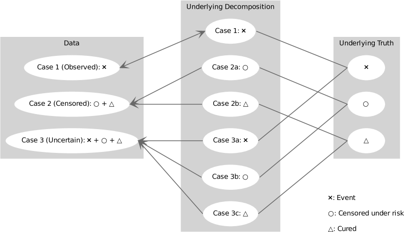
Figure 1: Decomposition of subjects in three different cases.

We propose an integrative Cox cure model with regularization to perform survival regression with uncertain events and a latent cure fraction. The model setup thus extends both the Cox model and the cure model. More specifically, our approach can be regarded as a mixture model with the regular Cox model as its skeleton, in which the event uncertainty and the cure status are modeled as latent variables with missing values. Regularized estimation techniques are utilized to enable shrinkage estimation and variable selection. We developed a computational algorithm based on an integration of the Majorization-Minimization algorithm, the profile likelihood, and the coordinate descent method. The algorithm was shown to be stable, efficient, and have monotonic descending property. Our new method outperformed competing methods in simulation studies under realistic settings similar to the motivating application of the suicide risk study.

The proposed approach was applied to study the risk of subsequent suicide attempt after suicide-related hospitalization for adolescent and young adult population, using medical claims data of year 2012 to 2017 from Connecticut All-Payer Claims Database (APCD). The identified risk factors are highly interpretable and consistent with current understanding; intriguingly, our method is able to distinguish the risk factors that are mostly helpful in assessing whether the patients are under risk of subsequent attempt and the ones that can actually predict the time of subsequent attempt. The predicted cure and event status among those uncertain suicide attempts identified by the E98x codes are further investigated, providing several new insights on suicide risk identification and prevention.

The rest of the paper is organized as follows. In Section 2, we describe the claims data and the problem setup for studying subsequent suicide attempt. In Section 3, based on a methodological review, we propose the integrative Cox cure model with uncertain events and derive its likelihood. The estimation procedure is developed in Section 4. Simulation studies are presented in Section 5. The suicide risk study is reported in Section 6. Section 7 concludes with a discussion.

2 Data and Exploratory Analysis

We focused on young patients of age 10–24 who were admitted to hospitals in Connecticut from 2012–2017 due to suicide attempts, whether determined or suspected. Data on primary and secondary diagnoses were available from the Connecticut APCD. We excluded a small proportion of patients with expired/dead status at discharge of their first recorded suicide-related hospitalization, and focused on those patients who survived and were discharged. The event of interest was a subsequent suicide attempt after the first hospitalization due to possible suicidal behaviors (diagnosed by E95x or E98x codes). The available APCD data was from October 1, 2012 to September 30, 2017. As such, we considered a retrospective follow-up study setup, in which the patients were followed up until a determined or suspected suicide attempt occurred or until September 20, 2017 if no suicide attempt was observed.

A total of 7,552 patients with prior hospitalizations for suicide attempts were included in this analysis. Among them, 3,831 patients were female and 3,721 patients were male. A total of 736 patients were coded as having subsequently attempted suicide using the E95x codes, while 173 patients experienced injuries whose cause was undetermined as to whether a suicide attempt or accident as indicated by the E98x diagnosis codes, and the remaining 6,643 subjects did not have a recorded suicide attempt during the follow-up. In other words, the size of Case 1–3 is, respectively, 736, 6,643, and 173. The censoring rate among subjects in Case 1–2 is 90.0%, and almost 20% of suicide attempts were identified with uncertainty.

The APCD data contained a large amount of information on the characteristics of patients and their previous hospital admissions. The diagnoses were mainly recorded as ICD-9 diagnosis codes prior to fiscal year 2015, and ICD-10 codes (the 10th Revision) were used afterwards. As the existing rules (Patrick et al., 2010; Chen and Aseltine, 2017) for identifying determined/suspected suicide attempts were mainly based on ICD-9 codes, we translated all the ICD-10 diagnosis codes to their ICD-9 equivalence by the General Equivalence Mappings developed from Centers by the Medicare and Medicaid Services. Both forward and backward mapping were used in the crosswalk as suggested by the Agency for Healthcare Research and Quality. The translation was efficiently done by R package touch (Wang et al., 2018).

After harmonizing to ICD-9 codes, we grouped the codes in the data by their three leading characters, which resulted in 911 major diagnosis categories. For each patient, we counted the number of appearances of the diagnosis codes belonging to each category in his/her historical records up to the initial admission. We further filtered out rare diagnosis codes to avoid separation/semi-separation problem by restricting minimum cell counts of the 2 by 2 contingency table of the diagnosis indicator and the event indicator of subjects in Case 1–2 to be at least 10. While this simple filtering approach is a common practice, we remark that it is possible to apply some newly developed feature aggregation methods (Yan and Bien, 2021; Chen et al., 2022) to better utilize very rare diagnosis codes. The remaining 246 ICD-9 categories, in addition to demographic covariate gender and age, were considered in the survival analysis predicting a subsequent attempt.

For subjects in Cases 1–2, the overall survival probability estimated by the Kaplan–Meier estimator (Kaplan and Meier, 1958) with point-wise confidence intervals (based on normality of the logarithm of survival rate estimates) is plotted in Figure 2. A flat tail was observed at the end of the survival curve, which suggested a long enough follow-up time and a possible presence of a cure fraction. We applied the method proposed by Maller and Zhou (1994) to formally test whether the follow-up is sufficient. The test statistic $a_{n}$ was proposed to be ${(1-N_{n}/n)}^{n}$, where $n$ is the sample size, $N_{n}$ is the number of uncensored observations in time period $(2T_{n}^{*}-T_{n},T_{n}^{*}]$, $T_{n}^{*}$ is the largest uncensored event time, and $T_{n}$ is the largest survival observed time. In our case, the test statistics $a_{n}$ computed based on the data excluding Case 3 is 0.25%, which suggested a strong evidence of a sufficient follow-up and motivated us to consider a potential cure fraction in the modeling. We further performed the likelihood ratio test proposed by Maller and Zhou (1995) for testing the presence of a cure fraction among patients in Case 1–2. More specifically, we fitted a regular Cox model and Cox cure model with age and gender as control variables to patients in Case 1–2, where the logistic part of the Cox cure model only included an intercept term. The test statistic was 3678.0, much larger than the critical value 2.71, which provided a strong evidence of the presence of a cure fraction among patients in Cases 1–2.

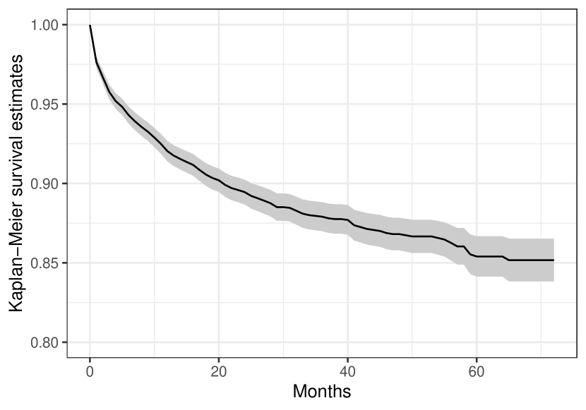
Figure 2: The overall survival curve by the Kaplan-Meier estimator for subjects in Cases 1–2.

The unique features of the problem demonstrated in our exploratory analysis motivate us to develop a general statistical approach on handling uncertain and rare medical diagnosis in time-to-event modeling.

3 Integrative Cox Cure Model with Uncertain Events

3.1 Overview of Existing Methods

In the literature, a few methods have been proposed to similar problems of mis-measured survival outcomes or uncertain events. When a binary diagnosis outcome was measured with uncertainty, Richardson and Hughes (2000) proposed an estimation procedure for the product limit estimate of survival function with no covariate based on the expectation maximization (EM) algorithm (Dempster et al., 1977). The method is only applicable for discrete-time contexts where the time points of outcome testing are predetermined. Meier et al. (2003) extended the discrete proportional hazards model (Kalbfleisch and Prentice, 2002) to mis-measured outcomes under a setting similar to Richardson and Hughes (2000) but allowed covariate effects. Wang et al. (2020) proposed a model for survival data with uncertain event times arising from partial linkage of different datasets, i.e., for a subject there could be multiple conflicting potential event times and censoring time, arising from linking different datasets without unique identifiers and among which only one of them is the truth. None of the above methods is appropriate for the uncertainty scenario in our problem, and none of them considered cure fraction and feature selection.

On the other hand, the cure rate model was first proposed by Berkson and Gage (1952). The logit link has been widely used in modeling the susceptible probability as proposed by Farewell (1982). Kuk and Chen (1992) proposed modeling the conditional survival times through a Cox proportional hazards model (Cox, 1972). Its model estimation based on the EM algorithm was later proposed by Sy and Taylor (2000). So far limited efforts have been made for survival data with masked events and the presence of a cure fraction. Dahlberg and Wang (2007) and Zhang and Wang (2009) proposed cure models with masked events based on the Cox model and the accelerated failure time (AFT) model (Wei, 1992), respectively, in the framework of competing risks. Unfortunately, neither of the above methods considered uncertain events, where no unmasking event is observed.

Regularization techniques are often adopted in practice to conduct feature selection with large data. Here our review shall mainly focus on the computational and methodological aspects of regularization that are related to survival analysis. Coordinate descent (CD) methods for solving the lasso problem (Tibshirani, 1996) was proposed by Fu (1998) and known as the “shooting” procedure. The CD algorithms for generalized linear models and Cox models were developed by Friedman et al. (2010) and Simon et al. (2011), respectively.However, as mentioned in Friedman et al. (2010), the convergence of Newton’s method used for handling non-quadratic loss is generally expected but not guaranteed. For regularized Cox model, Simon et al. (2011) used an approximated Hessian matrix of the (partial) log-likelihood, which also lacks convergence guarantee. To resolve these convergence issues, Yang and Zou (2013) derived the coordinate-majorization-descent (CMD) algorithm for the regularized Cox’s model, which combines the CD method with the principle of majorization-minimization (MM) algorithm (Hunter and Lange, 2004; Lange et al., 2000) and always converges. Recently, a few works have been proposed to perform variable selection for cure models. Scolas et al. (2016) proposed variable selection with adaptive lasso for interval-censored data in a parametric cure model. Masud et al. (2018) proposed variable selection methods for mixture cure model and promotion cure model. Some recent works on cure models have promoted structural similarity (Fan et al., 2017) and sign consistency (Shi et al., 2019) of covariate coefficient estimates on both model components of the cure model.

3.2 Proposed Method

Consider a random sample of $n$ subjects who fall into the three cases as illustrated in Figure 1. Let $I_{1}$, $I_{2}$, and $I_{3}$ be the indices of the subjects in Case 1, 2, and 3, respectively. Define $T_{j}=\min(V_{j},C_{j})$, $\Delta_{j}=\bm{1}(V_{j}\leq C_{j})$ with realizations $t_{j}$ and $\delta_{j}$, where $V_{j}$ and $C_{j}$ is random variable of the event time and the censoring time of subject $j$, $j\in\{1,\ldots,n\}$, respectively. The survival time $T_{j}$ is observed for all cases. However, the event indicator $\Delta_{j}$ is observed only for $j\in I_{1}\cup I_{2}$ but missing for $j\in I_{3}$. Let $\xi_{j}=\bm{1}(j\in I_{1}\cup I_{2})$ be an indicator variable taking value 1 if $\Delta_{j}$ is observed and taking value 0 otherwise. Define $Z_{j}=1$ if subject $j$ is susceptible (not cured), and $Z_{j}=0$ otherwise with probability $p_{j}=\Pr(Z_{j}=1)$. We assume that censoring time $C_{j}$ is independent of $Z_{j}$. Note that $Z_{j}=1$ is observed for $j\in I_{1}$ but missing for $j\in I_{2}\cup I_{3}$, which suggests that we observe $\xi_{j}=1$, $\Delta_{j}=1$, and $Z_{j}=1$ for $j\in I_{1}$. Given that $Z_{j}=0$, that $\Delta_{j}=0$ holds with probability one. For $j\in I_{2}$, we observe $\xi_{j}=1$ and $\Delta_{j}=0$. Suppose that the available data of subject $j$ are $\{(\bm{x}_{j}^{\top},t_{j},\sigma_{j},\xi_{j})\}$, where $\bm{x}_{j}$ is a $p$-dimensional covariate vector, the actual event indicator $\delta_{j}$ is masked by $\sigma_{j}=z_{j}\delta_{j}\xi_{j}$, and $z_{j}$ is the realization of $Z_{j}$. Given that $\xi_{j}=1$, we have $j\in I_{1}\cup I_{2}$ by definition and we observe $\sigma_{j}=1$ for $j\in I_{1}$, and $\sigma_{j}=0$ for $j\in I_{2}$. We assume $\delta_{j}$ is missing at random (MAR) satisfying

$$q_{j}:=\Pr(\xi_{j}=1\mid T_{j}=t_{j},\Delta_{j}=\delta_{j},Z_{j}=z_{j},\bm{x}_{j})=\Pr(\xi_{j}=1\mid T_{j}=t_{j},\bm{x}_{j}),$$

which means the event missing indicator $\xi_{j}$ depends on the fully observed $t_{j}$ and $\bm{x}_{j}$ only.

We regard the problem as a label-missing problem and give the likelihood function under the complete data as follows:

$$\prod_{j\in I_{1}}q_{j}p_{j}f(t_{j}\mid Z_{j}=1,\bm{x}_{j})\overline{G}(t_{j})\prod_{j\in I_{2}}q_{j}g(t_{j}){\left[p_{j}S(t_{j}\mid Z_{j}=1,\bm{x}_{j})\right]}^{z_{j}}{\left[(1-p_{j})\right]}^{1-z_{j}}$$

$$\prod_{j\in I_{3}}(1-q_{j}){\left[p_{j}f(t_{j}\mid Z_{j}=1,\bm{x}_{j})\overline{G}(t_{j})\right]}^{\delta_{j}z_{j}}{\left[p_{j}g(t_{j})S(t_{j}\mid Z_{j}=1,\bm{x}_{j})\right]}^{(1-\delta_{j})z_{j}}{\left[(1-p_{j})g(t_{j})\right]}^{1-z_{j}}$$

where $f(t\mid Z_{j}=1,\bm{x}_{j})$ and $S(t\mid Z_{j}=1,\bm{x}_{j})$ are the density function and survival function of $V_{j}$ given the covariates and that the subject $j$ is susceptible, respectively; $g(t)$ and $\overline{G}(t)$ are the density function and survival function of $C_{j}$, respectively. Due to the MAR assumption, we treat the likelihood contributions of the $\{\xi_{j}\}$ as nuisance components and simplify the complete-data likelihood function as follows:

$$\prod_{j\in I_{1}}p_{j}f(t_{j}\mid Z_{j}=1,\bm{x}_{j})\overline{G}(t_{j})\prod_{j\in I_{2}}g(t_{j}){\left[p_{j}S(t_{j}\mid Z_{j}=1,\bm{x}_{j})\right]}^{z_{j}}{\left[(1-p_{j})\right]}^{1-z_{j}}$$

$$\prod_{j\in I_{3}}{\left[p_{j}f(t\mid Z_{j}=1,\bm{x}_{j})\overline{G}(t_{j})\right]}^{\delta_{j}z_{j}}{\left[p_{j}g(t_{j})S(t_{j}\mid Z_{j}=1,\bm{x}_{j})\right]}^{(1-\delta_{j})z_{j}}{\left[(1-p_{j})g(t_{j})\right]}^{1-z_{j}},$$ (1)

which is useful for deriving an EM algorithm for computation. See Supplementary Materials for the derivation details.

Given that $Z_{j}=1$, we assume the event time $V_{j}$ of subject $j$ follows a Cox proportional hazards model (Cox, 1972) with the hazard function

$$h(t\mid Z_{j}=1,\bm{x}_{j})=h_{0}(t\mid Z_{j}=1)\exp(\bm{x}_{j}^{\top}\bm{\beta}),$$ (2)

where $h_{0}(\cdot\mid Z_{j}=1)$ is an unspecified baseline function for events, and $\bm{\beta}$ is a vector of unknown coefficient of the covariate vector $\bm{x}_{j}$. Then the conditional survival function of the event time of subject $j$ is $S(t\mid Z_{j}=1,\bm{x}_{j})=\exp\{-H_{0}(t\mid Z_{j}=1)\exp(\bm{x}_{j}^{\top}\bm{\beta})\}$, where $H_{0}(t\mid Z_{j}=1)=\int_{0}^{t}h_{0}(s\mid Z_{j}=1)\mathrm{d}s$ and the conditional density function is $f(t\mid Z_{j}=1,\bm{x}_{j})=h(t\mid Z_{j}=1,\bm{x}_{j})S(t\mid Z_{j}=1,\bm{x}_{j})$. Given that subject $j$ is cured ($Z_{j}=0$), the conditional survival function satisfies $S(t\mid Z_{j}=0,\bm{x}_{j})=1$, for $t<+\infty$.

Similarly, let $h_{c}(\cdot)$ denote the hazard function of censoring times and $H_{c}(t)=\int_{0}^{t}h_{c}(s)\mathrm{d}s$. Then $g(t)=h_{c}(t)\overline{G}(t)$ and $\overline{G}(t)=\exp\{-H_{c}(t)\}$. Here we assume the censoring time is independent of the event times and susceptible indicators conditional on the covariates $\bm{x}_{j}$. This conditional independence assumption of the censoring time is justified for our study because the censoring was administrative.

We utilize a logistic regression setup (Farewell, 1982) to model $p_{j}$ with an intercept and covariates $\bm{x}_{j}$’s. Here by allowing zero covariate coefficients, the same set of covariates is considered for modeling both the Cox regression part (2) and the cure probability part. The logistic model can be expressed as

$$\Pr(Z_{j}=1)=p_{j}=\frac{\exp(\bm{x}_{j}^{\top}\bm{\gamma}+\gamma_{0})}{1+\exp(\bm{x}_{j}^{\top}\bm{\gamma}+\gamma_{0})},$$ (3)

where $\gamma_{0}$ is the coefficient of the intercept term.

Let $\bm{\theta}=\left\{\bm{\gamma},\bm{\beta},\gamma_{0},h_{0}(\cdot\mid Z_{j}=1),h_{c}(\cdot)\right\}$ be the set of unknown parameters. Then from the complete-data likelihood in (3.2), by integrating out the missing components, the likelihood function under the observed data $\bm{Y}^{O}=\left\{\bm{Y}_{1},\bm{Y}^{O}_{2},\bm{Y}^{O}_{3}\right\}$ is

$$L(\bm{\theta}\mid\bm{Y}^{O})= \prod_{j\in I_{1}}\left[p_{j}f(t_{j}\mid Z_{j}=1,\bm{x}_{j})\overline{G}(t_{j})\right]$$

$$\prod_{j\in I_{2}}\left[p_{j}g(t_{j})S(t_{j}\mid Z_{j}=1,\bm{x}_{j})+(1-p_{j})g(t_{j})\right]$$

$$\prod_{j\in I_{3}}\large[p_{j}f(t_{j}\mid Z_{j}=1,\bm{x}_{j})\overline{G}(t_{j})+$$

$$~{}~{}~{}~{}~{}~{}p_{j}g(t_{j})S(t_{j}\mid Z_{j}=1,\bm{x}_{j})+(1-p_{j})g(t_{j})\large].$$ (4)

With the above likelihood derivations, we propose the following regularized likelihood estimator

$$\hat{\bm{\theta}}=\operatorname*{arg\,min}_{\bm{\theta}}-\frac{1}{n}\ell(\bm{\theta}\mid\bm{Y}^{O})+P(\bm{\theta};\lambda),$$ (5)

where $\ell(\bm{\theta}\mid\bm{Y}^{O})$ is the log-likelihood function under the observed data given in (3.2), and $P(\bm{\theta};\lambda)$ represents the penalty function for $\bm{\theta}$ with the tuning parameter $\lambda$. More specifically, we consider the elastic net penalties (Zou and Hastie, 2005) for both $\bm{\beta}$ and $\bm{\gamma}$, and let $P(\bm{\theta};\lambda)=P_{1}(\bm{\beta};\alpha_{1},\lambda_{1})+P_{2}(\bm{\gamma};\alpha_{2},\lambda_{2})$, where

$$P_{1}(\bm{\beta};\alpha_{1},\lambda_{1}) =\lambda_{1}\left(\alpha_{1}\sum_{k=1}^{p}\omega_{k}\lvert\beta_{k}\rvert+\frac{1-\alpha_{1}}{2}\sum_{k=1}^{p}\beta_{k}^{2}\right),$$

$$P_{2}(\bm{\gamma};\alpha_{2},\lambda_{2}) =\lambda_{2}\left(\alpha_{2}\sum_{k=1}^{p}\nu_{k}\lvert\gamma_{k}\rvert+\frac{1-\alpha_{2}}{2}\sum_{k=1}^{p}\gamma_{k}^{2}\right),$$

with tuning parameters ($\alpha_{1}$, $\lambda_{1}$) and ($\alpha_{2}$, $\lambda_{2}$) for $\bm{\beta}$ and $\bm{\gamma}$, respectively. In addition, the $\omega_{k}$ and $\nu_{k}$, $k=1,\ldots,p$, represent optional non-negative weights (Zou and Zhang, 2009). For example, in the low-dimensional case where the non-regularized estimators $(\bm{\beta}^{0},\bm{\gamma}^{0})$ are reliable, one could set $\omega_{k}=|\beta_{k}^{0}|^{-1}$ and $\nu_{k}=|\gamma_{k}^{0}|^{-1}$. In our study, we adopted unit weights $\omega_{k}=1$ and $\nu_{k}=1$ for simplicity.

4 Model Estimation

4.1 Computational Algorithm

We propose an estimation procedure to solve (5) by utilizing the architecture of the EM algorithm, in which the M-step adopts a profile likelihood similar to the partial likelihood (Cox, 1975) and the CMD algorithm (Yang and Zou, 2013).

We briefly describe the structure of the proposed algorithm. In the E-step, we compute the conditional expectation of the complete-data log-likelihood given the observed data and estimates from the last step. In the M-step, the conditional expectation of the complete-data log-likelihood are decomposed into several parts that involve exclusive sets of parameters. Specifically, after the hazard functions are profiled out using “Breslow estimator” (Breslow, 1974) and the idea of partial likelihood of Cox (1975), the problem boils down to two parts involving $\bm{\beta}$ and ($\bm{\gamma}$,$\gamma_{0}$), respectively. We adopt the monotonic quadratic approximation (Böhning and Lindsay, 1988) and derive CMD algorithms (Yang and Zou, 2013) for optimizing these two sub-problems. We show the descending properties of the proposed updating steps and consequently conclude that our proposed algorithm enjoys the monotonic descending property in principle of an MM algorithm.

We summarize the resulting EM algorithm in Algorithm 1, with the sub-routine algorithms of $\bm{\beta}$, and ($\bm{\gamma}$,$\gamma_{0}$) in Algorithms 2 and 3, respectively. To simplify the notations, we define $h_{j}:=h(t_{j}\mid Z_{j}=1,\bm{x}_{j})$, $S_{j}:=S(t\mid Z_{j}=1,\bm{x}_{j})$. Most necessary quantities are defined within Algorithm 1. We define some additional quantities below. For simplicity, the dependency on the last step estimates is omitted. The M-step objective functions for $\bm{\beta}$ and ($\bm{\gamma}$,$\gamma_{0}$) are respectively

$$J(\bm{\beta}) =-\frac{1}{n}l(\bm{\beta})+P_{1}(\bm{\beta};\alpha_{1},\lambda_{1}),$$ (6)

$$J(\bm{\gamma},\gamma_{0}) =-\frac{1}{n}l(\bm{\gamma},\gamma_{0})+P_{2}(\bm{\gamma};\alpha_{2},\lambda_{2}),$$ (7)

where

$$l(\bm{\beta}) =\sum_{j=1}^{n}\int_{0}^{\infty}I_{j}(\bm{\beta},t)\mathrm{d}N_{j}(t),$$

$$I_{j}(\bm{\beta},t) =\bm{x}_{j}^{\top}\bm{\beta}-\log\left[\sum_{j=1}^{n}\bm{1}(t\leq t_{j})M_{j}\exp(\bm{x}_{j}^{\top}\bm{\beta})\right],$$

$$N_{j}(t) =\bm{1}(t_{j}\leq t)\left[\bm{1}(j\in I_{1})+w_{j,1}\bm{1}(j\in I_{3})\right],$$

$$l(\bm{\gamma},\gamma_{0}) =\sum_{j=1}^{n}(\bm{x}_{j}^{\top}\bm{\gamma}+\gamma_{0})M_{j}-\log\left[1+\exp(\bm{x}_{j}^{\top}\bm{\gamma}+\gamma_{0})\right],$$

$$M_{j} =\bm{1}(j\in I_{1})+v_{j}\bm{1}(j\in I_{2})+(w_{j,1}+w_{j,2})\bm{1}(j\in I_{3}),$$

$$v_{j} =p_{j}S_{j}/[p_{j}S_{j}+(1-p_{j})],$$

$$m_{j} =p_{j}h_{j}S_{j}\overline{G}_{j}+p_{j}S_{j}g_{j}+(1-p_{j})g_{j},$$

$$w_{j,1} =p_{j}h_{j}S_{j}\overline{G}_{j}/m_{j},~{}w_{j,2}=p_{j}S_{j}g_{j}/m_{j}.$$

Let $\dot{l}_{k}(\bm{\beta})$ and $\dot{l}_{k^{\prime}}(\bm{\gamma},\gamma_{0})$ denote the first partial derivative of $l(\bm{\beta})$ and $l(\bm{\gamma},\gamma_{0})$ with respect to $\beta_{k}$ and $\gamma_{k^{\prime}}$, respectively, where $k\in\{1,\ldots,p\}$ and $k^{\prime}\in\{0,\ldots,p\}$. Define

$$D_{k}=\frac{1}{4n}\sum_{j=1}^{n}\int_{0}^{\infty}{\left[\max_{j\in\mathcal{R}(t)}(x_{j,k})-\min_{j\in\mathcal{R}(t)}(x_{j,k})\right]}^{2}\mathrm{d}N_{j}(t),~{}B_{k}=\frac{1}{4n}\sum_{j=1}^{n}x_{j,k}^{2},$$

where $\mathcal{R}(t)=\{j\mid Y_{j}(t)=1\}$ represents the index set of subjects in the risk-set at time $t$. See Supplementary Materials for details.

Algorithm 1 Estimation procedure for the proposed model.

initialize $\bm{\beta}$, $\bm{\gamma}$, $\gamma_{0}$, $h_{0}(\cdot\mid Z_{j}=1)$, and $h_{c}(\cdot)$;

repeat 

    for $j=1,2,\ldots,n$ do $\triangleright$ The E-step

$$p_{j} \leftarrow\frac{1}{1+\exp(-\bm{x}_{j}^{\top}\bm{\gamma}+\gamma_{0})};$$

$$S_{j} \leftarrow\exp\left[-\sum_{s\leq t_{j}}h_{0}(s\mid Z_{j}=1)\exp(\bm{x}^{\top}_{j}\bm{\beta})\right];~{}\overline{G}_{j}\leftarrow\exp\left[-\sum_{s\leq t_{j}}h_{c}(s)\right];$$

$$m_{j,1} \leftarrow p_{j}h_{j}S_{j}\overline{G}_{j};~{}m_{j,2}\leftarrow p_{j}h_{c}S_{j}\overline{G}_{j};~{}m_{j,3}\leftarrow(1-p_{j})h_{c}\overline{G}_{j};~{}v_{j}\leftarrow\frac{m_{j,2}}{m_{j,2}+m_{j,3}};$$

         for $k=1,2,3$ do

$$w_{j,k}\leftarrow\frac{m_{j,k}}{\sum_{k=1}^{3}m_{j,k}};$$

         end for 

$$M_{j}\leftarrow\bm{1}(j\in I_{1})+v_{j}\bm{1}(j\in I_{2})+(w_{j,1}+w_{j,2})\bm{1}(j\in I_{3});$$

    end for 

    for each $t\in\mathcal{T}_{2}\cup\mathcal{T}_{3}$ do $\triangleright$ The M-step of $h_{c}(\cdot)$

$$C(t) \leftarrow\sum_{j=1}^{n}\bm{1}(t_{j}\leq t)\bm{1}(j\in I_{2})+(w_{j,2}+w_{j,3})\bm{1}(t_{j}\leq t)\bm{1}(j\in I_{3});$$

$$h_{c}(t) \leftarrow\frac{\mathrm{d}C(t)}{\sum_{j=1}^{n}Y_{j}(t)};$$

    end for 

    for each $t\in\mathcal{T}_{1}\cup\mathcal{T}_{3}$ do $\triangleright$ The M-step of $h_{0}(\cdot\mid Z_{j}=1)$

$$N(t) \leftarrow\sum_{j=1}^{n}\bm{1}(t_{j}\leq t)\bm{1}(j\in I_{1})+w_{j,1}\bm{1}(t_{j}\leq t)\bm{1}(j\in I_{3});$$

$$h_{0}(t\mid Z_{j}=1) \leftarrow\frac{\mathrm{d}N(t)}{\sum_{j=1}^{n}\bm{1}(t\leq t_{j})M_{j}\exp(\bm{x}_{j}^{\top}\bm{\beta})};$$

    end for 

    go to Algorithm 2 $\triangleright$ The M-step of $\bm{\beta}$

    go to Algorithm 3 $\triangleright$ The M-step of $\bm{\gamma}$ and $\gamma_{0}$

until Convergence of $\bm{\beta}$, $\bm{\gamma}$, and $\gamma_{0}$

Algorithm 2 The M-step of $\bm{\beta}$.

input: $\bm{\beta}$ from last EM iteration

repeat 

    for $k=1,\ldots,p$ do $\triangleright$ update $\beta_{k}$

$$\beta_{k}\leftarrow\frac{s(D_{k}\beta_{k}+\frac{1}{n}\dot{l}_{k}(\bm{\beta}),\lambda_{1}\alpha_{1}\omega_{k})}{D_{k}+\lambda_{1}(1-\alpha_{1})},$$

      where $s(a,b)={(\lvert a\rvert-b)}_{+}\mathrm{sign}(a)$ is the soft-thresholding operator.

    end for 

until Convergence of $\bm{\beta}$

Algorithm 3 The M-step of $\bm{\gamma}$ and $\gamma_{0}$.

input: $\bm{\gamma}$ and $\gamma_{0}$ from last EM iteration;

repeat 

    do $\triangleright$ update $\gamma_{0}$

$$\gamma_{0}\leftarrow\gamma_{0}+\frac{4}{n}\dot{l}_{0}(\bm{\gamma},\gamma_{0});$$

    for $k=1,\ldots,p$ do $\triangleright$ update $\gamma_{k}$

$$\gamma_{k}\leftarrow\frac{s(B_{k}{\gamma}_{k}+\frac{1}{n}\dot{l}_{k}(\bm{\gamma},\gamma_{0}),\lambda_{2}\alpha_{2}\nu_{k})}{B_{k}+\lambda_{2}(1-\alpha_{2})},$$

      where $s(a,b)={(\lvert a\rvert-b)}_{+}\mathrm{sign}(a)$ is the soft-thresholding operator.

    end for 

until Convergence of $\bm{\gamma}$ and $\gamma_{0}$

4.2 Initialization, Tail Completion, and Tuning

We propose a simple yet pragmatic initialization procedure for the proposed EM algorithm:

• Setting the event indicators of subjects in Case 3 to be 0.5, fit a regular logistic model on event indicators and use the estimated coefficients to initialize $\hat{\bm{\gamma}}$ and $\hat{\gamma_{0}}$;

• Fit a regular Cox model on all the certain events (Case 1) and use the estimated coefficients to initialize $\hat{\bm{\beta}}$; For subject $j$, $j\in\{1,\ldots,n\}$, initialize $\hat{S}_{j}$ with the fitted survival function evaluated at $t_{j}$; initialize $\hat{h}_{j}$ with a nearest left neighbor interpolation of the fitted hazard function (if no left neighbor, use nearest right neighbor).

• Switching event and censoring for all the certain records (Case 1–2), estimate the hazard function for censoring by the Nelson-Aalen estimator (without covariates) and obtain the corresponding survival function estimate; initialize $\hat{\overline{G}}_{j}$ with the fitted survival function evaluated at $t_{j}$; initialize $\hat{h}_{c}(t_{j})$ with a nearest left neighbor interpolation of the fitted hazard function (if no left neighbor, use nearest right neighbor).

The initialization procedure was applied in the simulation studies presented in Section 5 and the results were satisfactory in all scenarios. In addition, we applied the zero tail completion (Sy and Taylor, 2000) in the E-steps when updating the conditional survival function of event times to avoid identifiability issue of cure models (Li et al., 2001; Hanin and Huang, 2014), which imposes the constraint that $S_{0}(t^{*}\mid Z=1)=0$ for any $t^{*}$ greater than the largest event time onto the baseline survival function $S_{0}(t)$.

We select the tuning parameters, $(\lambda_{1},\alpha_{1},\lambda_{2},\alpha_{2})$, through a grid search. To be more specific, we generate an equally-spaced decreasing sequence in logarithm scale of the tuning parameters, $\lambda_{1}$ and $\lambda_{2}$, respectively, from the smallest values that produce all zero coefficients for the corresponding model component. Similarly, we can select $\alpha_{1}$ and $\alpha_{2}$, respectively, from an equally-spaced sequence between 0 and 1; in practice it is also common to simply set them as some constant close to 1. As we have multiple tuning parameters, we propose to use the Bayesian information criteria (BIC) for computational efficiency. In particular, we adopted the BIC for censored survival models (Volinsky and Raftery, 2000), where the penalty term is proportional to the effective sample size, i.e., number of uncensored observations, instead of number of observations. Alternatively, one may select the final model by K-fold cross-validation, where the observation with the largest event time must always stay in the training set to avoid numerical issue due to zero-tail completion. However, the tuning procedure using cross-validation can be much more computationally intensive than using the BIC.

We have made our implementation of the proposed methods available in a user-friendly R package intsurv, which can be accessed at https://cran.r-project.org/package=intsurv.

5 Simulation Study

5.1 Setup and Data Generation

We designed simulation settings to mimic our suicide risk application. The main concern was the estimation/prediction performance of the proposed model and its ability to distinguish the true events among the uncertain events.

The simulated dataset consisted of subjects in three different cases as illustrated in Figure 1. Accordingly, we first generated the survival data with a cure fraction, which served as the ground truth. Then we randomly assigned each subject to different cases from its ground truth. To be more specific, for each subject who actually has observed event, we assigned it randomly to Case 1 with probability $p_{1}$, or Case 3a with probability $1-p_{1}$. For each susceptible subject whose event time was censored, we randomly assign it to Case 2a with probability $p_{2}$, or Case 3b with probability $1-p_{2}$. For each cured subject, we randomly assign it to Case 2b with probability $p_{3}$, or Case 3c with probability $1-p_{3}$. A diagram of the data generation is provided in Supplementary Materials.

In the following simulation settings, we fixed the size of Case 1 and Case 2 to be approximately 100 and 1,900, respectively. The censoring rate among these certain records (Case 1–2) was thus about 95%, which simulated the severe censoring in the real suicide risk data. The size of Case 3 was set to be 100 or 200, i.e., the same or twice of the size of Case 1, which resulted in the sample size being 2,100 or 2,200, respectively. Within Case 3, we set the proportion of Case 3a to be 30% or 70%, respectively. The value of $p_{1}$ could then be computed as the size ratio of Case 3a to Case 1. For simplicity, we let $p_{2}=p_{3}$. Thus, the size ratio of Case 2 to Case 3b & Case 3c could be computed as $p_{2}/(1-p_{2})$, which determined the value of $p_{2}$ (and $p_{3}$).

We generated susceptible indicators from logistic model with an intercept term. We set the coefficient of the intercept term to $-0.847$ or $0.847$ so that the baseline cure rate (when all covariates are zeros) was 70% or 30%, respectively. For susceptible subjects, the event times were generated from Weibull-Cox model with baseline hazard function $h_{0}(t;\bm{x})=0.2t\exp(\bm{x}^{\top}\bm{\beta})$; For cured subjects, the event times were set to be infinity. The censoring times were generated independently with the event times from exponential distribution truncated at 10. The rate parameter of the truncated exponential distribution is tuned so that the desired case’s decomposition was attained.

The different specification on the baseline cure rate, the size of Case 3, and the proportion of Case 3a resulted in totally eight different simulation scenarios. More specifically, the size of Case 3 was set to be the same with the size of Case 1 in the scenario (1) to (4) and twice in the scenario (5) to (8); The proportion of Case 3a was set to be 30% in the scenario (1), (2), (5), and (6), and 70% in the remaining scenarios; The baseline cure rate was set to be 30% in scenarios (1), (3), (5), and (7), and 70% in the remaining scenarios. We applied these eight scenarios to a low-dimensional setting ($p=8$) without regularization and a large-dimensional setting ($p=100$) with regularization in Section 5.4 and Section 5.5, respectively. The number of replicates for each scenario was 1,000.

5.2 Competing Methods

The proposed method is denoted by I.Cure. We considered three competing approaches based on the Cox cure rate model. The first approach (denoted by Cure1) fits the Cox cure model to those certain records (Case 1–2) only, which simply excludes subjects with uncertain events. The second approach (denoted by Cure2) fits the Cox cure model for all subjects, where subjects having uncertain events in Case 3 are all treated as censored. In contrast, the third method (denoted by Cure3) fits the Cox cure model by taking the uncertain events all as actual events ignoring their uncertainty. We did not include the Cox models as they performed worse than their corresponding Cox cure rate models in the presence of a cure fraction.

We also included an oracle procedure (denoted by O.Cure) based on Cox cure rate model where the true event indicators in Case 3 were all given. The oracle procedure is infeasible in practice, but it provides a reference on the best achievable performances in the comparison.

5.3 Evaluation Metrics

For both model components, we measured the estimation performance by the $\ell_{2}$-norm of $(\hat{\bm{\beta}}-\bm{\beta}^{0})$, i.e., $\|\hat{\bm{\beta}}-\bm{\beta}^{0}\|={[{(\hat{\bm{\beta}}-\bm{\beta}^{0})}^{\top}(\hat{\bm{\beta}}-\bm{\beta}^{0})]}^{1/2}$, where $\hat{\bm{\beta}}$ and $\bm{\beta}^{0}$ represent the estimated covariate coefficients and the underlying true covariate coefficients, respectively.

For subject $j$ in Case 3, we took estimated posterior probability $w_{j,1}$ from Algorithm 1, i.e., the estimated probability of subject $j$ having actual event at time $t_{j}$, for the identification of uncertain events. We also computed the oracle posterior probability based on Bayes rule for such identification using the underlying true models and simulated datasets, providing references of the best achievable performances. Given the simulated true event indicators in Case 3, we were able to evaluate the identification correctness by the area under curve (AUC) of the receiver operating characteristic curve (ROC).

For large-dimensional models, we were interested in the variable selection performance of regularized estimation. The performance was measured by the true positive rate (TPR) among those non-zero coefficients and the false positive rate (FPR) among those zero coefficients, which were defined as follows:

$$\mathrm{TPR}=\frac{\sum_{k=1}^{p}\bm{1}(\hat{\beta}_{k}\neq 0)\bm{1}(\beta_{k}^{0}\neq 0)}{\sum_{k=1}^{p}\bm{1}(\beta_{k}^{0}\neq 0)},~{}\mathrm{FPR}=\frac{\sum_{k=1}^{p}\bm{1}(\hat{\beta}_{k}\neq 0)\bm{1}(\beta_{k}^{0}=0)}{\sum_{k=1}^{p}\bm{1}(\beta_{k}^{0}=0)},$$

where $\beta_{k}^{0}$ is the $k$-th underlying truth covariate coefficient, and $\hat{\beta}_{k}$ is the $k$-th estimated covariate coefficient from the regularized estimation procedure.

5.4 Setting 1

In Setting 1, we considered $p=8$ covariates, $x_{k}$, $k\in\{1,\ldots,8\}$, that were randomly generated from multivariate normal distribution with marginal means zero and variances one. The correlation between $x_{k}$ and $x_{l}$, $k\neq l$, was set to be $\rho^{\lvert k-l\rvert}$, where $\rho=0.2$. We considered two overlapped but different sets of covariates in the logistic model and the Weibull-Cox model. The covariates $x_{4}$–$x_{8}$ were used in the logistic model for generating the susceptible indicators for each subject. For susceptible subjects, the covariates $x_{1}$–$x_{5}$ were used in the Weibull Cox model for generating event times. The underlying true non-zero covariate coefficients were fixed to be $\bm{\beta}^{0}=\bm{\gamma}^{0}={(0.8,0.5,1,0.3,0.6)}^{\top}$ in both parts. We assumed that the underlying true sets of covariates were both known in the low-dimensional settings. In other words, among eight covariates, only $x_{1}$–$x_{5}$ were considered in the Cox model (2) and only $x_{4}$–$x_{8}$ were considered in the logistical model (3), and no regularization was applied in all methods.

The estimation results are presented in Table 1, which show that I.Cure gave better estimation performance in both model parts than those competing methods and close performance compared with the oracle method in almost all 8 scenarios. In addition, the AUC’s on identifying the true events from uncertain records were about 75% using I.Cure, about 13% lower than those from the oracle method across all scenarios; the detailed results are presented in Supplementary Materials.

Table 1: Simulation results of Setting 1: comparison on parameter estimation performance for the incidence part and the latency part, respectively, through mean of $\|\hat{\bm{\gamma}}-\bm{\gamma}^{0}\|$ and $\|\hat{\bm{\beta}}-\bm{\beta}^{0}\|$ (with the standard deviation given in parenthesis).

	$\|\hat{\bm{\gamma}}-\bm{\gamma}^{0}\|$						$\|\hat{\bm{\beta}}-\bm{\beta}^{0}\|$
#	O.Cure	I.Cure	Cure1	Cure2	Cure3		O.Cure	I.Cure	Cure1	Cure2	Cure3
1	1.05	1.17	1.28	1.37	1.20		0.26	0.29	0.31	0.33	0.70
	(0.42)	(0.45)	(0.43)	(0.44)	(0.54)		(0.10)	(0.11)	(0.12)	(0.12)	(0.10)
2	0.57	0.69	0.74	0.78	1.17		0.28	0.30	0.33	0.34	0.71
	(0.21)	(0.28)	(0.26)	(0.26)	(0.37)		(0.09)	(0.10)	(0.12)	(0.12)	(0.11)
3	0.86	1.11	1.39	1.54	0.87		0.23	0.30	0.33	0.35	0.38
	(0.33)	(0.40)	(0.41)	(0.41)	(0.38)		(0.08)	(0.11)	(0.12)	(0.13)	(0.10)
4	0.47	0.70	0.88	0.95	0.63		0.24	0.30	0.34	0.35	0.39
	(0.17)	(0.27)	(0.26)	(0.26)	(0.21)		(0.08)	(0.10)	(0.12)	(0.12)	(0.11)
5	0.93	1.15	1.35	1.52	1.34		0.24	0.29	0.33	0.35	0.87
	(0.35)	(0.45)	(0.45)	(0.44)	(0.65)		(0.08)	(0.10)	(0.11)	(0.12)	(0.08)
6	0.48	0.68	0.79	0.89	1.62		0.24	0.28	0.32	0.34	0.87
	(0.17)	(0.27)	(0.25)	(0.25)	(0.43)		(0.08)	(0.10)	(0.12)	(0.12)	(0.08)
7	0.65	1.03	1.54	1.81	0.75		0.19	0.33	0.36	0.38	0.44
	(0.23)	(0.35)	(0.38)	(0.38)	(0.27)		(0.07)	(0.12)	(0.12)	(0.13)	(0.08)
8	0.35	0.74	1.09	1.22	0.78		0.19	0.30	0.35	0.37	0.47
	(0.12)	(0.27)	(0.23)	(0.22)	(0.20)		(0.06)	(0.11)	(0.12)	(0.13)	(0.11)

We estimated the standard error estimates based on inter-quartile range and normal approximation. To check the performance of the proposed method in making inferences about the unknown covariate coefficients, we used bootstrap with 200 bootstrap samples. The mean of standard error (SE) estimates and the empirical SEs for the coefficient of all covariates are presented in Supplementary Materials. The bootstrap SE estimates were close to the empirical SEs of the coefficient estimates in most of the settings.

5.5 Setting 2

Table 2: Simulation results of Setting 2: comparison on variable selection performance for the logistic model part and Cox model part through mean of true positive rate (TPR) and false positive rate (FPR) in percentage (with the standard deviation given in parenthesis).

		Logistic						Cox
#	Measure	O.Cure	I.Cure	Cure1	Cure2	Cure3		O.Cure	I.Cure	Cure1	Cure2	Cure3
1	TPR	22.0	29.3	24.3	22.0	7.4		95.4	93.5	89.5	89.6	92.1
		(29.7)	(31.1)	(25.3)	(12.5)	(33.3)		(13.1)	(21.4)	(7.9)	(13.2)	(19.9)
	FPR	1.14	1.93	1.52	1.40	0.41		3.29	4.14	2.98	2.96	2.41
		(1.96)	(2.70)	(3.16)	(0.66)	(2.44)		(2.68)	(3.07)	(3.68)	(2.03)	(2.80)
2	TPR	70.5	66.2	66.5	65.7	29.5		94.7	92.9	89.6	87.6	89.5
		(29.4)	(35.3)	(27.3)	(29.1)	(31.7)		(16.7)	(19.0)	(17.1)	(7.9)	(24.8)
	FPR	2.42	3.06	2.54	2.61	0.73		3.24	4.50	3.20	3.18	3.05
		(2.44)	(1.39)	(2.68)	(2.51)	(2.47)		(3.46)	(2.51)	(2.98)	(2.82)	(2.69)
3	TPR	29.1	42.3	29.7	26.3	17.0		97.5	96.6	90.0	87.0	97.5
		(29.0)	(33.7)	(30.6)	(28.0)	(32.1)		(21.7)	(7.6)	(19.8)	(17.3)	(4.7)
	FPR	1.17	2.35	1.67	1.60	0.63		3.40	4.29	3.16	2.89	3.16
		(2.29)	(1.90)	(2.77)	(3.55)	(1.08)		(2.77)	(2.58)	(2.90)	(4.54)	(2.26)
4	TPR	80.6	81.8	74.1	68.3	61.2		97.3	97.2	90.5	87.8	96.4
		(28.5)	(33.1)	(38.8)	(28.8)	(21.3)		(22.3)	(10.6)	(9.0)	(17.6)	(3.6)
	FPR	2.42	3.64	2.82	2.55	1.42		3.10	4.40	3.09	2.99	3.29
		(2.18)	(2.55)	(2.03)	(2.64)	(2.24)		(2.66)	(3.46)	(2.79)	(2.75)	(2.25)
5	TPR	27.5	36.1	26.6	24.3	3.4		97.4	95.2	91.8	88.7	95.0
		(17.9)	(30.6)	(33.3)	(29.9)	(14.6)		(19.4)	(20.3)	(9.1)	(21.7)	(5.1)
	FPR	1.12	2.39	1.37	1.42	0.15		3.34	5.30	3.23	3.07	2.26
		(1.17)	(2.29)	(1.83)	(2.67)	(3.41)		(2.18)	(2.86)	(2.66)	(2.68)	(4.61)
6	TPR	79.1	73.9	72.4	69.3	15.0		97.3	94.2	90.3	87.6	93.9
		(32.7)	(29.5)	(30.5)	(27.7)	(20.8)		(11.8)	(24.8)	(15.1)	(12.9)	(13.2)
	FPR	2.43	3.82	2.67	2.60	0.26		3.10	5.62	2.92	2.77	3.45
		(2.57)	(2.39)	(2.62)	(0.85)	(2.59)		(2.84)	(2.64)	(4.03)	(2.37)	(2.61)
7	TPR	43.9	61.3	42.4	31.0	21.7		99.2	98.8	89.4	85.7	98.9
		(32.7)	(27.9)	(29.8)	(38.2)	(22.8)		(17.7)	(7.8)	(19.1)	(3.8)	(18.2)
	FPR	1.15	3.22	1.94	1.72	0.45		3.47	5.38	3.05	2.85	3.29
		(2.97)	(1.33)	(2.07)	(1.62)	(2.72)		(3.79)	(2.24)	(2.83)	(2.65)	(2.47)
8	TPR	90.9	91.7	82.1	76.1	62.6		99.4	98.7	92.3	87.9	98.6
		(32.2)	(29.4)	(28.6)	(31.4)	(41.8)		(19.5)	(7.0)	(22.5)	(5.9)	(5.2)
	FPR	2.19	4.23	2.80	2.67	1.32		2.49	5.49	2.66	2.41	3.33
		(2.65)	(2.44)	(2.15)	(2.81)	(2.08)		(3.06)	(2.82)	(2.73)	(4.04)	(2.64)

In Setting 2, we increased the number of covariates to 100. The covariates were randomly generated from multivariate normal distribution with marginal means zero and variances one. The correlation between $x_{k}$ and $x_{l}$, $k\neq l$, $k,l\in\{1,\ldots,100\}$, was set to be $\rho^{\lvert k-l\rvert}$, where $\rho=0.2$. For $x_{1}$–$x_{8}$, we considered a same set of covariate coefficients in the low-dimensional settings. We set the coefficients of the remaining covariates to be all zero. We conducted the proposed regularized estimation approach with the estimation criteria given in (5). The number of the grid points was set to be 10 for both $\lambda_{1}$ and $\lambda_{2}$, which resulted in a 10 by 10 two-dimensional grid. The minimum tuning parameter was set to be 0.1 of the smallest value that produces all zero coefficients. For simplicity, we set $\alpha_{1}=\alpha_{2}=1$.

The variable selection results are summarized in Table 2. The TPR’s from I.Cure were evidently greater than those from the competing methods under almost all the settings for both model components. On the other hand, the FPR’s from I.Cure were only slightly larger than those from the competing methods. Overall, I.Cure gave considerably high TPR’s compared with the oracle method at a cost of slightly high FPR’s.

In addition, we investigated the prediction performance of different methods using an out-of-sample procedure. The results show that I.Cure led to consistently better out-of-sample AUC for the prediction of susceptibility and better out-of-sample C-index for the prediction of survival time than the competing methods in all the scenarios. We also considered using adaptive weights and obtained similar results compared to using unit weights. The detailed results are provided in Supplementary Materials.

6 Understanding Subsequent Suicide Attempts with Uncertain Diagnosis Records

We applied the proposed method and three competing methods to the Connecticut suicide attempt data. The elastic-net penalization was used because some predictors could be highly correlated. Our main interests were to (1) identify relevant diagnosis categories that were predictive of subsequent suicide attempts after the initial hospitalization due to suicidal behaviors, (2) verify that the proposed integrative approach has the potential of improving predictive power over methods that do not address uncertainty, and (3) investigate the suspected attempts among subjects in Case 3, to understand which injuries of undetermined intent were more likely self-inflicted.

Risk factor selection

The odds ratio and hazard ratio estimates from the proposed method and those competing ones are summarized in Table 3, in which we also report the prevalence of each selected ICD-9 category in each of the three cases of patients. Several ICD-9 categories related to mental health and drug abuse were selected by the different approaches. As expected, the prevalence of each selected ICD-9 category is the highest among Case 1 patients and the lowest among Case 2 patients. The number of variables selected in the incidence part for modeling susceptible status ranged from 6 to 11, while only 1 to 2 variables were selected for modeling the conditional time-to-event distribution. This suggests that understanding the timing of suicide is generally a much harder problem than understanding its occurrence.

Table 3: Suicide risk study: prevalence of selected ICD-9 categories in three cases of patients and the exponentiated coefficient estimates (hazard or odd ratios) from different approaches.

	Prevalence %			I.Cure		Cure1		Cure2		Cure3
ICD-9	$I_{1}$	$I_{2}$	$I_{3}$	$e^{\hat{\bm{\gamma}}}$	$e^{\hat{\bm{\beta}}}$	$e^{\hat{\bm{\gamma}}}$	$e^{\hat{\bm{\beta}}}$	$e^{\hat{\bm{\gamma}}}$	$e^{\hat{\bm{\beta}}}$	$e^{\hat{\bm{\gamma}}}$	$e^{\hat{\bm{\beta}}}$	Description
296	55.3	26.0	29.4	1.78		1.80		1.77		1.77		Episodic mood disorders
298	19.2	7.6	8.9	1.08				1.06		1.01		Other Nonorganic Psychoses
300	47.6	25.8	28.3	1.10		1.04		1.10		1.02		Anxiety, Dissociative and Somatoform Disorders
301	13.9	4.6	5.6	1.32		1.22		1.32		1.21		Personality disorders
304	12.4	4.0	5.3	1.31	1.01	1.11		1.17		1.60		Drug Dependence
312	8.7	3.0	3.7	1.10				1.10		1.06		Disturbance of Conduct, Not Elsewhere Classified
313	6.8	2.2	2.7	1.23		1.01		1.19		1.15		Disturbance of Emotions Specific to Childhood and Adolescence
319	1.6	0.3	0.4	1.02				1.21				Unspecified intellectual disabilities
507	6.2	2.6	3.0							1.05		Pneumonitis Due to Solids and Liquids
564	31.8	12.6	14.8	1.02				1.04		1.02		Functional Digestive Disorders, Not Elsewhere Classified
977	1.8	0.4	0.6							1.05		Poisoning by Other and Unspecified Drugs and Medicinal Substances
V62	24.7	14.5	16.2	1.31	1.01	1.32	1.00	1.33	1.02	1.25	1.00	Other Psychosocial Circumstances

There were 6 ICD-9 predictors selected by all methods in the incidence part. We found that these results were well supported by existing literature. In particular, all models suggested that patients with personality disorders (ICD-9 301) had a higher risk of being susceptible and making further suicide attempts. Among these patients, about 35.2% had borderline personality disorder (ICD-9 301.83) and 15.9% had chronic depressive personality disorder (ICD-9 301.12) in our data. Similar finding had been reported by e.g., Harris and Barraclough (1997), Lieb et al. (2004) and McGirr et al. (2007), among others. Another interesting selected ICD-9 category was V62 indicating psychosocial circumstances. The majority (66.3%) of the patients with V62 had suicide ideations (ICD-9 V62.84), which was one of the conditions for identifying determined suicide attempts in addition to the E95 codes. Among patients with suicide ideation diagnosis, about 88.2% were diagnosed at the initial hospitalization, which strongly suggested that initial hospitalization could provide important information relevant to the prevention of further suicide attempts. Other commonly selected ICD-9 categories were related to mood disorders (ICD-9 296), anxiety (ICD-9 300), drug dependence (ICD-9 304), and disturbance of emotions (313), which are well known to be important suicide risk factors. Besides the aforementioned 6 categories, our proposed method selected 4 more, including nonorganic psychoses (ICD-9 298), disturbance of conduct (ICD-9 312), unspecified intellectual disabilities (ICD-9 319), and functional digestive disorders (ICD-9 564). The associations between these conditions and suicide risk are well supported by existing studies (Falcone et al., 2010; Linker et al., 2012; Ludi et al., 2012; Spiegel et al., 2007). In our data, we found that among patients whose event times were censored, 59.8% of them were without any of these 10 conditions identified by the incidence part of our model. As such, these patients could be regarded as with the least risk of having subsequent suicide attempt. Our findings could help clinical practice for a better allocation of the limited resource for suicide prevention.

Our proposed method selected drug dependence (ICD-9 304) and psychosocial diagnoses (ICD-9 V62) in both the incidence part and the latency part, which suggested that these two conditions not only increased the probability of being susceptible to subsequent suicide attempt after the initial hospitalization but also associated with a reduced time to subsequent attempt. On the other hand, the other three naive methods all missed the selection of drug dependence. The link between drug dependence and suicide attempt is well known in children and adolescents (Berman and Schwartz, 1990; Doshi et al., 2020; Luo et al., 2022), and suicide death is recognized as a major component of the ongoing opioid crisis by the National Institute on Drug Abuse.

We also attempted to conduct post-selection inference on the I.Cure model. To this end, we simply refitted the selected model without regularization and performed bootstrap to obtain 95% confidence intervals of the coefficient estimates. According to Zhao et al. (2021), such a naive two-step procedure could still yield asymptotically valid inference under certain conditions. The results are shown in Supplementary Materials. Indeed, most of the predictors were significant except ICD-9 298, 300, and V62 in the incidence part.

Prediction performance

We evaluated the model prediction performance based on the selected variables from those different approaches by a random splitting procedure. To be more specific, we randomly split subjects in Case 1–2, respectively, into a training set with probability 0.6 and a test set with probability 0.4. The number of subjects in Case 1 and Case 2 in the testing set is thus 294 and 2,657, respectively. The proposed method was fitted to the split training set and Case 3, while for the Cure1 method, only the split training set was utilized. By definition, the Cure2 method and the Cure3 method took uncertain events in Case 3 as censoring and actual events, respectively. The procedure was repeated 1,000 times.

We applied the time-varying sensitivity and specificity estimator proposed by Uno et al. (2007) to evaluate the prediction performance based on the estimated survival probabilities over the test set that consists of Case 1–2 only. We focused on short-term survival in the first 4 months when about 40% of subjects in Case 3 had observed time. Motivated by the clinical setting, in which suicide related interventions would not be universally implemented but be targeted on those at highest risk, we evaluated the predictive performance within an estimated high-risk group of small size.

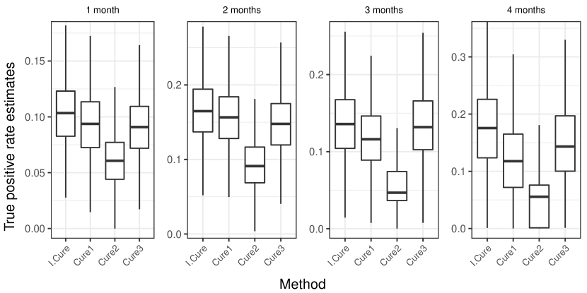
Figure 3: Suicide risk study: boxplot matrix of true positive rate of predicting 1–4 months survival with the proportion of high-risk group controlled at 5%.

Figure 3 provides a visual comparison of the prediction performance for 1–4 month’s survival when the proportion of the high risk group is controlled at 5% of the population. The TPR from the I.Cure method was the largest in the first four months compared with those competing methods. The Cure1 and Cure3 method provided the second largest TPR in the first two month and last two months, respectively, while the Cure2 method always gave the worst performance in the first four months.

Understanding suspected attempts

We then investigated the suspected attempts in Case 3, to understand which injuries of undetermined intent were more likely to be self-inflicted. The estimated posterior probabilities were used to classify whether these patients had actual attempts, censored events, or cured using the Bayes’ rule. Among those 173 patients in Case 3 with injury of undetermined origin, 36 (20.8%) patients were classified as having an actual events (determined suicide attempts), 137 (79.1%) patients were classified as being cured, and none of the patients were classified as being censored under risk. The result was consistent with our early conclusion on the sufficient follow-up period.

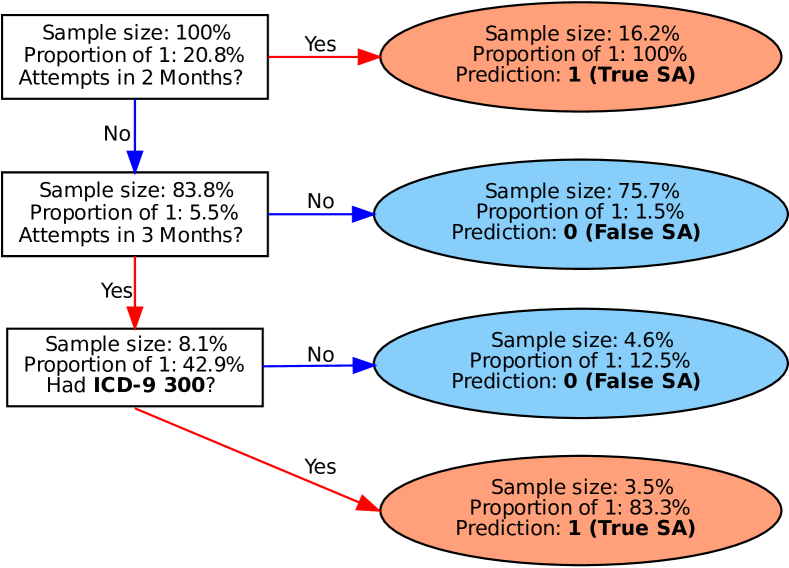
(a) Model with survival times

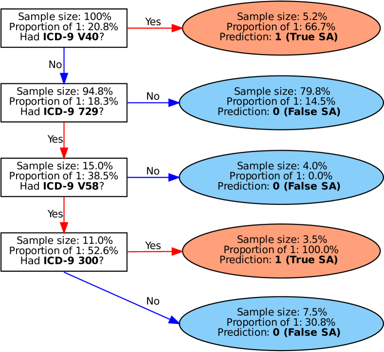
(b) Model without survival times

Figure 4: Suicide risk study: classification trees of actual suicide attempts (SA) among subjects having undetermined SA based on identified Case 3a among Case 3 from I.Cure.

Given the identified subjects in Case 3a from I.Cure, we fitted two classification tree models with a regular complexity pruning procedure among subjects in Case 3 to further explore ICD-9 categories that predict Case 3a. Figure 4 provides their visualization.

In tree model (a), we included the survival times of the suspected suicide attempt as one of the predictors. The results show that the patients who have had undetermined suicide attempts within 2 months (accounting for 16.2% of patients) after the initial hospitalization were very likely to have made actual suicide attempts. On the other hand, those patients who have not made a suspected attempt within 3 months (accounting for 75.7% of patients) were unlikely to have made actual suicide attempts. Among the remaining (8.1%) patients, those having anxiety, dissociative, and somatoform disorders (ICD-9 300) were predicted to have had an actual suicide attempt. Then, in tree model (b), we excluded the survival times to see how well we could use historical information to predict Case 3a. In the root node, patients having mental and behavioral problems (ICD-9 V40) were predicted to have had actual suicide attempts. In the second node, the remaining (94.8%) patients without disorders of soft tissues (ICD-9 729) were predicted to not have had actual suicide attempts. About 85% of patients were classified to the corresponding terminal nodes by the first two nodes. For the remaining (15.0%) patients, those who required continued care after initial treatment (ICD-9 V58) and had anxiety, dissociative, and somatoform disorders (ICD-9 300) were predicted to have had actual attempts.

Out of 36 identified cases, model (a) was able to capture 34 of them, while model (b) only captured 15, which suggested that the estimated baseline hazard functions from I.Cure based on observations in Case 1 and Case 2 played an important role in identifying Case 3a. Our analysis provided the compositions of these suspected suicide events, which could be insightful and further examined by domain experts for a more effective suicide prevention strategy among youth and young adults.

Another interesting question is that, among all the actual attempts, why some were coded as determined while some were coded as suspected? That is, how to distinguish the subjects in Case 1 and the identified subjects in Case 3a? We fitted a classification tree model for these two sets of subjects. The fitted model suggested that subjects having prior poisoning by unspecified biological substances (ICD-9 979), or general symptoms (ICD-9 780), such as physiological exhaustion (ICD-9 780.79), unspecified altered mental status (ICD-9 780.97) were more likely to be recorded as having suspected suicide attempts with E98 codes.

7 Discussion

We have examined a general modeling setup for survival data with the presence of a cure fraction and uncertain events indicators. In our application, we obtained insightful results on potential risk factors associated with both the occurrence and timing of subsequent suicide attempt following initial suicide-related hospitalization among adolescents. Several important risk factors might have been missed by the other naive approaches that improperly treat uncertain diagnosis records. We thoroughly examined the estimated cure and event status among those subjects with suspected suicide attempt diagnosis, which provided important insights on how to identify the true suicidal events among them and how to utilize such uncertain records in predictive modeling of suicide.

Several directions are worth pursuing for future research. For the proposed method, the relative risk on the conditional latency is specified by a Cox proportional hazards model, which may be restrictive. It is interesting to consider testing procedures of the proportional hazard assumption in the presence of outcome uncertainty and cure fraction (Wileyto et al., 2013), and develop other more flexible models to relax the proportional hazards assumption. In the estimation procedure, we applied in the E-steps the zero tail completion, which essentially treats the subjects who have survived after the largest uncensored event time as not susceptible. This may be too restricted in some applications. It is worth exploring other methods such as exponential and Weibull tail completion (Peng, 2003) to model the tail of the conditional survival curve. In fact, we tried exponential tail completion in our simulation studies in Section 5 and obtained very similar results from using zero tail completion.

Given the prevalence of uncertainty in the identification of medical conditions from diagnosis codes, we believe our approach can be broadly applied to improve many studies on health conditions with real-world claims data.

Conflict of Interest

None.

Supplementary Material

A Derivation of Likelihood Functions

To simplify the notations, we let $p(\cdot)$ be a generic notation representing the probability density function. For discrete random variables, we can still view $p(\cdot)$ as the density function by the adoption of counting measure.

We derive both the complete-data likelihood and the corresponding observed-data likelihood. Firstly, for subject $j\in I_{1}$, we observe that $T_{j}=V_{j}$ and $\sigma_{j}=\delta_{j}=Z_{j}=\xi_{j}=1$; no label is missing. Thus, the likelihood contribution can be derived as follows:

$$p(T_{j}=t_{j},\Delta_{j}=1,\xi_{j}=1,Z_{j}=1)$$

$$=~{} p(\xi_{j}=1,T_{j}=t_{j},\Delta_{j}=1\mid Z_{j}=1)p(Z_{j}=1)$$

$$=~{} p(\xi_{j}=1\mid T_{j}=t_{j},\Delta_{j}=1,Z_{j}=1)p(T_{j}=t_{j},\Delta_{j}=1\mid Z_{j}=1)p(Z_{j}=1)$$

$$=~{} p(\xi_{j}=1\mid T_{j}=t_{j})p(T_{j}=t_{j},\Delta_{j}=1\mid Z_{j}=1)p(Z_{j}=1)$$

$$=~{} q_{j}p_{j}f_{j}(t_{j})\overline{G}(t_{j}),$$

where $q_{j}=p(\xi_{j}=1\mid T_{j}=t_{j})$, $f_{j}(t)$ is the density function of $V_{j}$ given that the subject $j$ is susceptible, and $\overline{G}(t)$ is the survival function of $C_{j}$.

Secondly, for subject $j\in I_{2}$, we observe $T_{j}=C_{j}$, $\Delta_{j}=0$, and $\xi_{j}=1$. But $Z_{j}$ is not observed. We have

$$p(T_{j}=t_{j},\Delta_{j}=0,\xi_{j}=1\mid Z_{j}=1)$$

$$=~{} p(\xi_{j}=1\mid T_{j}=t_{j},\Delta_{j}=0,Z_{j}=1)p(T_{j}=t_{j},\Delta_{j}=0\mid Z_{j}=1)$$

$$=~{} p(\xi_{j}=1\mid T_{j}=t_{j})p(C_{j}=t_{j},V_{j}>C_{j}\mid Z_{j}=1)$$

$$=~{} q_{j}g(t_{j})S_{j}(t_{j}),$$

$$p(T_{j}=t_{j},\Delta_{j}=0,\xi_{j}=1\mid Z_{j}=0)$$

$$=~{} p(\xi_{j}=1\mid T_{j}=t_{j},\Delta_{j}=0,Z_{j}=0)p(T_{j}=t_{j},\Delta_{j}=0\mid Z_{j}=0)$$

$$=~{} p(\xi_{j}=1\mid T_{j}=t_{j})p(C_{j}=t_{j},V_{j}>C_{j}\mid Z_{j}=0)$$

$$=~{} q_{j}g(t_{j}),$$

where $g(t)$ is the density function of $C_{j}$, $S_{j}(t)$ is the survival function of $V_{j}$ given that the subject $j$ is susceptible. Therefore, the observed-data likelihood contribution of subject $j$ is

$$p(T_{j}=t_{j},\Delta_{j}=0,\xi_{j}=1)= \sum_{z_{j}\in\{0,1\}}p(T_{j}=t_{j},\Delta_{j}=0,\xi_{j}=1\mid Z_{j}=z_{j})p(Z_{j}=z_{j})$$

$$=~{} q_{j}g(t_{j})[p_{j}S_{j}(t_{j})+(1-p_{j})],$$

and the likelihood contribution under the complete data is

$$p(T_{j}=t_{j},\Delta_{j}=0,\xi_{j}=1,Z_{j}=z_{j})=q_{j}g(t){\left[p_{j}S_{j}(t_{j})\right]}^{z_{j}}{\left[(1-p_{j})\right]}^{1-z_{j}}.$$

Lastly, for subject $j\in I_{3}$, we only observe uncertain event time $T_{j}=\min(V_{j},C_{j})$ with $\xi_{j}=0$. Neither $\Delta_{j}$ nor $Z_{j}$ is observable. We can obtain the likelihood contribution of subject $j$ in Case 3a and Case 3b under the observed data as follows:

$$p(T_{j}=t_{j},\xi_{j}=0\mid Z_{j}=1)$$

$$=~{} p(T_{j}=t_{j},\xi_{j}=0,\delta_{j}=0\mid Z_{j}=1)+p(T_{j}=t_{j},\xi_{j}=0,\delta_{j}=1\mid Z_{j}=1)$$

$$=~{} p(\xi_{j}=0\mid T_{j}=t_{j},\Delta_{j}=1,Z_{j}=1)p(T_{j}=t_{j},\Delta_{j}=1\mid Z_{j}=1)+$$

$$p(\xi_{j}=0\mid T_{j}=t_{j},\Delta_{j}=0,Z_{j}=1)p(T_{j}=t_{j},\Delta_{j}=0\mid Z_{j}=1)$$

$$=~{} p(\xi_{j}=0\mid T_{j}=t_{j})\left[p(V_{j}=t_{j},C_{j}\geq V_{j}\mid Z_{j}=1)+p(C_{j}=t_{j},V_{j}>C_{j}\mid Z_{j}=1)\right]$$

$$=~{} (1-q_{j})\left[f_{j}(t_{j})\overline{G}(t_{j})+g(t_{j})S_{j}(t_{j})\right],$$

and thus

$$p(T_{j}=t_{j},\xi_{j}=0,Z_{j}=1)= p(T_{j}=t_{j},\xi_{j}=0\mid Z_{j}=1)p(Z_{j}=1)$$

$$= (1-q_{j})p_{j}\left[f_{j}(t_{j})\overline{G}(t_{j})+g(t_{j})S_{j}(t_{j})\right].$$

Similarly, as for the subject $j$ in Case 3c, we can derive the observed data likelihood contribution as follows:

$$p(T_{j}=t_{j},\xi_{j}=0\mid Z_{j}=0)$$

$$=~{} p(T_{j}=t_{j},\xi_{j}=0,\delta_{j}=0\mid Z_{j}=0)$$

$$=~{} p(\xi_{j}=0\mid T_{j}=t_{j},\Delta_{j}=0,Z_{j}=0)p(T_{j}=t_{j},\Delta_{j}=0\mid Z_{j}=0)$$

$$=~{} p(\xi_{j}=0\mid T_{j}=t_{j})p(C_{j}=t_{j},V_{j}>C_{j}\mid Z_{j}=1)$$

$$=~{} (1-q_{j})g(t_{j}),$$

and thus

$$p(T_{j}=t_{j},\xi_{j}=0,Z_{j}=0)= p(T_{j}=t_{j},\xi_{j}=0\mid Z_{j}=0)p(Z_{j}=0)$$

$$= (1-q_{j})g(t_{j})(1-p_{j}).$$

Notice that $\Pr(\Delta_{j}=1\mid Z_{j}=0)=0$. Therefore, the observed data likelihood contribution for subject $j$ in Case 3 is

$$p(T_{j}=t_{j},\xi_{j}=0)=~{} (T_{j}=t_{j},\xi_{j}=0,Z_{j}=1)+p(T_{j}=t_{j},\xi_{j}=0,Z_{j}=0)$$

$$=~{} (1-q_{j})p_{j}\left[f_{j}(t_{j})\overline{G}(t_{j})+g(t_{j})S_{j}(t_{j})\right]+(1-q_{j})g(t_{j})(1-p_{j}),$$

and the likelihood contribution under the complete data is

$$p(T_{j}=t_{j},\Delta_{j}=\delta_{j},\xi_{j}=0,Z_{j}=z_{j})$$

$$=~{} (1-q_{j}){\left[p_{j}f_{j}(t_{j})\overline{G}(t_{j})\right]}^{\delta_{j}z_{j}}{\left[p_{j}g(t_{j})S_{j}(t_{j})\right]}^{(1-\delta_{j})z_{j}}{\left[(1-p_{j})g(t_{j})\right]}^{1-z_{j}}.$$

From the derived likelihood contributions for Case 1–3, we write down the likelihood functions under the complete data as follows:

$$\prod_{j\in I_{1}}q_{j}p_{j}f_{j}(t_{j})\overline{G}(t_{j})\prod_{j\in I_{2}}q_{j}g(t){\left[p_{j}S_{j}(t_{j})\right]}^{z_{j}}{\left[(1-p_{j})\right]}^{1-z_{j}}$$

$$\prod_{j\in I_{3}}(1-q_{j}){\left[p_{j}f_{j}(t_{j})\overline{G}(t_{j})\right]}^{\delta_{j}z_{j}}{\left[p_{j}g(t_{j})S_{j}(t_{j})\right]}^{(1-\delta_{j})z_{j}}{\left[(1-p_{j})g(t_{j})\right]}^{1-z_{j}}.$$

In addition, the missing at random assumption of the $\{\xi_{j}\}$ suggests that the likelihood contributions of $\{\xi_{j}\}$ do not involve $\{\delta_{j}\}$ or $\{z_{j}\}$, and thus can be treated as nuisance components that play no role in estimating the parameters of interest. As a result, the derived EM algorithm for those parameters of interest in next section do not depend on the ${q_{j}}$ at all.

Therefore, the simplified complete-data likelihood function and the corresponding observed-data likelihood function are, respectively, as follows:

$$\prod_{j\in I_{1}}p_{j}f_{j}(t_{j})\overline{G}(t_{j})\prod_{j\in I_{2}}g(t){\left[p_{j}S_{j}(t_{j})\right]}^{z_{j}}{\left[(1-p_{j})\right]}^{1-z_{j}}$$

$$\prod_{j\in I_{3}}{\left[p_{j}f_{j}(t_{j})\overline{G}(t_{j})\right]}^{\delta_{j}z_{j}}{\left[p_{j}g(t_{j})S_{j}(t_{j})\right]}^{(1-\delta_{j})z_{j}}{\left[(1-p_{j})g(t_{j})\right]}^{1-z_{j}},$$

and

$$\prod_{j\in I_{1}}p_{j}f_{j}(t_{j})\overline{G}(t_{j})\prod_{j\in I_{2}}g(t){\left[p_{j}S_{j}(t_{j})+(1-p_{j})\right]}$$

$$\prod_{j\in I_{3}}{\left[p_{j}f_{j}(t_{j})\overline{G}(t_{j})+p_{j}g(t_{j})S_{j}(t_{j})(1-p_{j})g(t_{j})\right]}.$$

B Derivation of Model Estimation Procedure

B.1 Derivation of the E-step

There is no missing indicators for subjects in Case 1. So we only need to derive the E-step for subjects in Case 2 and Case 3, respectively. For subjects in Case 2, the log-likelihood function under the complete data $\bm{Y}_{2}$ is

$$\ell(\bm{\theta}\mid\bm{Y}_{2})$$

$$= \sum_{j\in I_{2}}\log{g(t_{j})}+z_{j}\left(\log{p_{j}}+\log{S_{j}(t_{j}\mid Z_{j}=1)}\right)+(1-z_{j})\log{(1-p_{j})}$$

$$= \sum_{j\in I_{2}}z_{j}\left[(\bm{x}_{j}^{\top}\bm{\gamma}+\gamma_{0})-H_{0}(t_{j}\mid Z_{j}=1)\exp(x_{j}^{\top}\bm{\beta})\right]-\log\left[1+\exp(\bm{x}_{j}^{\top}\bm{\gamma}+\gamma_{0})\right]$$

$$+\log h_{c}(t_{j})-H_{c}(t_{j}).$$

Let $\bm{\theta}^{(i)}$ denote the set of parameter estimates at the $i$-th iteration. Given the observed data of subject $j$ in Case 2 and $\bm{\theta}^{(i)}$, by Bayes rule we have

$$\mathbb{E}\,(Z_{j}\mid T_{j}=t_{j},\Delta_{j}=0,\xi_{j}=1,\bm{\theta}^{(i)}) =\Pr(Z_{j}=1\mid T_{j}=t_{j},\Delta_{j}=0,\xi_{j}=1,\bm{\theta}^{(i)})$$

$$=\frac{\Pr(Z_{j}=1,T_{j}=t_{j},\Delta_{j}=0,\xi_{j}=1\mid\bm{\theta}^{(i)})}{\sum_{z_{j}\in\{0,1\}}p(Z_{j}=z_{j},T_{j}=t_{j},\Delta_{j}=0,\xi_{j}=1\mid\bm{\theta}^{(i)})}$$

$$=\frac{p_{j}^{(i)}S_{j}^{(i)}}{p_{j}^{(i)}S_{j}^{(i)}+(1-p_{j}^{(i)})}.$$

where $p_{j}^{(i)}$ and $S_{j}^{(i)}$ are the estimate of $p_{j}$ and $S_{j}(t_{j}\mid Z_{j}=1)$ at the $i$-th iteration, respectively. Let $\bm{Y}^{O}_{2}$ denote the observed data for subjects in Case 2. The E-step for subjects in Case 2 is as follows:

$$\mathbb{E}\,\ell(\bm{\theta}\mid\bm{Y}^{O}_{2},\bm{\theta}^{(i)})$$

$$= \sum_{j\in I_{2}}v_{j}^{(i)}\left[(\bm{x}_{j}^{\top}\gamma+\gamma_{0})-H_{0}(t_{j}\mid Z_{j}=1)\exp(x_{j}^{\top}\bm{\beta})\right]-\log\left[1+\exp(\bm{x}_{j}^{\top}\gamma+\gamma_{0})\right]$$

$$+\log h_{c}(t_{j})-H_{c}(t_{j}),$$

where $v_{j}^{(i)}=p_{j}^{(i)}S_{j}^{(i)}/[p_{j}^{(i)}S_{j}^{(i)}+(1-p_{j}^{(i)})]$.

Similarly, for subjects in Case 3, the log-likelihood function under the complete data is

$$\ell(\bm{\theta}\mid\bm{Y}_{3})$$

$$= \sum_{j\in I_{3}}\delta_{j}z_{j}\left[\log p_{j}+\log f_{j}(t_{j}\mid Z_{j}=1)+\log\overline{G}(t_{j})\right]$$

$$+(1-\delta_{j})z_{j}\left[\log p_{j}+\log g(t_{j})+\log S_{j}(t_{j}\mid Z_{j}=1)\right]+(1-z_{j})\left[\log(1-p_{j})+\log g(t_{j})\right].$$

Define $m_{j,k}^{(i)}$, $k\in\{1,2,3\}$, as follows:

$$m_{j,1}^{(i)}:=p(\Delta_{j}=1,Z_{j}=1,T_{j}=t_{j},\xi_{j}=0\mid\bm{\theta}^{(i)}) =q_{j}^{(i)}p_{j}^{(i)}h_{j}^{(i)}S_{j}^{(i)}\overline{G}_{j}^{(i)},$$

$$m_{j,2}^{(i)}:=p(\Delta_{j}=0,Z_{j}=1,T_{j}=t_{j},\xi_{j}=0\mid\bm{\theta}^{(i)}) =q_{j}^{(i)}p_{j}^{(i)}S_{j}^{(i)}g_{j}^{(i)},$$

$$m_{j,3}^{(i)}:=p(\Delta_{j}=0,Z_{j}=0,T_{j}=t_{j},\xi_{j}=0\mid\bm{\theta}^{(i)}) =q_{j}^{(i)}(1-p_{j}^{(i)})g_{j}^{(i)},$$

where $h_{j}^{(i)}$, $g_{j}^{(i)}$, and $\overline{G}_{j}^{(i)}$ are the estimate of $h_{j}(t_{j}\mid Z_{j}=1)$, $g(t_{j})$, and $\overline{G}_{j}(t_{j})$ at the $i$-th iteration, respectively. Let $m_{j}^{(i)}=\sum_{k=1}^{3}m_{j,k}^{(i)}$ and define $w_{j,k}^{(i)}$, $k\in\{1,2,3\}$, as follows:

$$w_{j,1}^{(i)} :=\mathbb{E}\,(\Delta_{j}Z_{j}\mid T_{j}=t_{j},\xi_{j}=0,\bm{\theta}^{(i)})=m_{j,1}^{(i)}/m_{j}^{(i)},$$

$$w_{j,2}^{(i)} :=\mathbb{E}\,\left[(1-\Delta_{j})Z_{j}\mid T_{j}=t_{j},\xi_{j}=0,\bm{\theta}^{(i)}\right]=m_{j,2}^{(i)}/m_{j}^{(i)},$$

$$w_{j,3}^{(i)} :=\mathbb{E}\,(1-Z_{j}\mid T_{j}=t_{j},\xi_{j}=0,\bm{\theta}^{(i)})=m_{j,3}^{(i)}/m_{j}^{(i)}.$$

The E-step for subjects in Case 3 is then given below.

$$\mathbb{E}\,\ell(\bm{\theta}\mid\bm{Y}^{O}_{3},\bm{\theta}^{(i)})$$

$$= \sum_{j\in I_{3}}w_{j,1}^{(i)}\left[\log h_{0}(t_{j}\mid Z_{j}=1)+\bm{x}^{\top}_{j}\bm{\beta}\right]+\left(w_{j,1}^{(i)}+w_{j,2}^{(i)}\right)\left[\bm{x}_{j}^{\top}\gamma+\gamma_{0}-H_{0}(t\mid Z_{j}=1)\exp(\bm{x}_{j}^{\top}\bm{\beta})\right]$$

$$-\log\left[1+\exp(\bm{x}_{j}^{\top}\gamma+\gamma_{0})\right]+\left(w_{j,2}^{(i)}+w_{j,3}^{(i)}\right)\log h_{c}(t_{j})-H_{c}(t_{j}).$$

B.2 Derivation of the M-step

The conditional expectation of the complete-data log-likelihood given the observed data and estimates from last step can be decomposed into several parts that involve exclusive sets of parameters.

First of all, the part involving $h_{c}(\cdot)$ is

$$\mathbb{E}\,\ell(h_{c}(\cdot)\mid\bm{Y}^{O},\bm{\theta}^{(i)})=\sum_{j=1}^{n}-H_{c}(t_{j})+\sum_{j\in I_{2}}\log h_{c}(t_{j})+\sum_{j\in I_{3}}(w_{j,2}^{(i)}+w_{j,3}^{(i)})\log h_{c}(t_{j}).$$ (8)

Because $H_{c}(t)$ is a non-decreasing function, $h_{c}(t)$ maximizing (8) is a discrete function that takes non-zero values at $t_{j}$, $j\in I_{2}\cup I_{3}$. Let $Y_{j}(t)=\bm{1}(t\leq t_{j})$ denote the at-risk indicator. Define that $C_{j,2}(t)=\bm{1}(t_{j}\leq t)\bm{1}(j\in I_{2})$, $C_{j,3}(t;\bm{\theta}^{(i)})=(w_{j,2}^{(i)}+w_{j,3}^{(i)})\bm{1}(t_{j}\leq t)\bm{1}(j\in I_{3})$, and $C(t;\bm{\theta}^{(i)})=\sum_{j=1}^{n}C_{j,2}(t)+C_{j,3}(t;\bm{\theta}^{(i)})=\sum_{j\in I_{2}}C_{j,2}(t)+\sum_{j\in I_{3}}C_{j,3}(t;\bm{\theta}^{(i)})$, and let $\mathrm{d}C(t;\bm{\theta}^{(i)})=C(t;\bm{\theta}^{(i)})-C(t-0;\bm{\theta}^{(i)})$ denote the jump size of $C(t;\bm{\theta}^{(i)})$. Then we may rewrite (8) to allow ties in $t_{j}$, $j\in I_{2}\cup I_{3}$ as

$$\mathbb{E}\,\ell(h_{c}(\cdot)\mid\bm{Y}^{O},\bm{\theta}^{(i)})=\sum_{t\in\mathcal{T}_{2}\cup\mathcal{T}_{3}}\left[\mathrm{d}C(t;\bm{\theta}^{(i)})\log h_{c}(t)-h_{c}(t)\sum_{j=1}^{n}Y_{j}(t)\right],$$ (9)

where $\mathcal{T}_{k}=\{t_{j}\mid j\in I_{k}\}$. Maximizing (9) gives that

$$h_{c}^{(i+1)}(t)=\frac{\mathrm{d}C(t;\bm{\theta}^{(i)})}{\sum_{j=1}^{n}Y_{j}(t)}.$$

Secondly, the part involving both $h_{0}(\cdot\mid Z_{j}=1)$ and $\bm{\beta}$ is

$$\mathbb{E}\,\ell(\bm{\beta},h_{0}(\cdot\mid Z_{j}=1)\mid\bm{Y}^{O},\bm{\theta}^{(i)})$$

$$= ~{}\sum_{j\in I_{1}}\bm{x}_{j}^{\top}\bm{\beta}+\log h_{0}(t_{j}\mid Z_{j}=1)-H_{0}(t_{j}\mid Z_{j}=1)\exp(\bm{x}_{j}^{\top}\bm{\beta})$$

$$+\sum_{j\in I_{2}}v_{j}^{(i)}\left[-H_{0}(t_{j}\mid Z_{j}=1)\exp(\bm{x}_{j}^{\top}\bm{\beta})\right]$$

$$+\sum_{j\in I_{3}}w_{j,1}^{(i)}\left[\bm{x}_{j}^{\top}\bm{\beta}+\log h_{0}(t_{j}\mid Z_{j}=1)\right]+\left(w_{j,1}^{(i)}+w_{j,2}^{(i)}\right)\left[-H_{0}(t_{j}\mid Z_{j}=1)\exp(\bm{x}_{j}^{\top}\bm{\beta})\right].$$ (10)

Similarly, $h_{0}(t\mid Z_{j}=1)$ maximizing (10) is a discrete function that takes non-zero values at $t_{j}$, $j\in I_{1}\cup I_{3}$. Define that $M_{j}^{(i)}=\bm{1}(j\in I_{1})+v_{j}^{(i)}\bm{1}(j\in I_{2})+(w_{j,1}^{(i)}+w_{j,2}^{(i)})\bm{1}(j\in I_{3})$, $N_{j}^{(i)}=\bm{1}(j\in I_{1})+w_{j,1}^{(i)}\bm{1}(j\in I_{3})$, $N_{j}(t;\bm{\theta}^{(i)})=\bm{1}(t_{j}\leq t)N_{j}^{(i)}$, and $N(t;\bm{\theta}^{(i)})=\sum_{j=1}^{n}N_{j}(t;\bm{\theta}^{(i)})$. Let $\mathrm{d}N(t;\bm{\theta}^{(i)})=N(t;\bm{\theta}^{(i)})-N(t-0;\bm{\theta}^{(i)})$ denote the jump size of $N(t;\bm{\theta}^{(i)})$. Then we may rewrite (10) to allow ties in $t_{j}$, $j\in I_{1}\cup I_{3}$ as

$$\mathbb{E}\,\ell(\bm{\beta},h_{0}(\cdot\mid Z_{j}=1)\mid\bm{Y}^{O},\bm{\theta}^{(i)})$$

$$= \sum_{t\in\mathcal{T}_{1}\cup\mathcal{T}_{3}}\mathrm{d}N(t;\bm{\theta}^{(i)})\log h_{0}(t\mid Z_{j}=1)-h_{0}(t\mid Z_{j}=1)\left[\sum_{j=1}^{n}Y_{j}(t)M_{j}^{(i)}\exp(\bm{x}_{j}^{\top}\bm{\beta})\right]$$

$$+\sum_{j=1}^{n}N_{j}^{(i)}\bm{x}_{j}^{\top}\bm{\beta}.$$ (11)

Maximizing (B.2) with regards to $h_{0}(t\mid Z_{j}=1)$ gives

$$h_{0}^{(i+1)}(t\mid Z_{j}=1)=\frac{\mathrm{d}N(t;\bm{\theta}^{(i)})}{\sum_{j=1}^{n}Y_{j}(t)M_{j}^{(i)}\exp(\bm{x}_{j}^{\top}\bm{\beta})},$$ (12)

which is similar to the “Breslow estimator” (Breslow, 1974) for the regular Cox model. Plugging (12) into (B.2) gives the profiled expectation,

$$\mathbb{E}\,\ell(\bm{\beta},h_{0}^{(i+1)}(\cdot\mid Z_{j}=1)\mid\bm{Y}^{O},\bm{\theta}^{(i)})=\sum_{t\in\mathcal{T}_{1}\cup\mathcal{T}_{3}}\mathrm{d}N(t;\bm{\theta}^{(i)})\left[\log\mathrm{d}N(t;\bm{\theta}^{(i)})-1\right]+\ell(\bm{\beta}\mid\bm{\theta}^{(i)}),$$

where

$$\ell(\bm{\beta}\mid\bm{\theta}^{(i)}) =\sum_{j=1}^{n}\int_{0}^{\infty}I_{j}(\bm{\beta},t\mid\bm{\theta}^{(i)})\mathrm{d}N_{j}(t;\bm{\theta}^{(i)}),$$ (13)

$$I_{j}(\bm{\beta},t\mid\bm{\theta}^{(i)}) =\bm{x}_{j}^{\top}\bm{\beta}-\log\left[\sum_{j=1}^{n}Y_{j}(t)M_{j}^{(i)}\exp(\bm{x}_{j}^{\top}\bm{\beta})\right].$$

This profiling approach is similar to the partial likelihood of Cox (1975) except that the susceptible indicators and the distribution of the censoring time come into play through $M_{j}^{(i)}$ and $\mathrm{d}N_{j}(t;\bm{\theta}^{(i)})$.

Thirdly, the part involving $\bm{\gamma}$ and $\gamma_{0}$ is

$$\mathbb{E}\,\ell(\bm{\gamma},\gamma_{0}\mid\bm{Y}^{O},\bm{\theta}^{(i)})=\sum_{j=1}^{n}(\bm{x}_{j}^{\top}\bm{\gamma}+\gamma_{0})M_{j}^{(i)}-\log\left[1+\exp(\bm{x}_{j}^{\top}\bm{\gamma}+\gamma_{0})\right],$$ (14)

which is similar to the log-likelihood function of a regular logistic regression model. For ease of notation, we henceforth denote (14) by $\ell(\bm{\gamma},\gamma_{0}\mid\bm{\theta}^{(i)})$.

Without regularization, maximizing (13) with respect to $\bm{\beta}$ and maximizing (14) with respect to $\bm{\gamma}$ and $\gamma_{0}$ can be done by the Newton-Raphson algorithm or its variants, in a similar fashion to the Cox model and the logistic regression model, respectively. In our implementation, we adopted the monotonic quadratic approximation algorithm proposed by Böhning and Lindsay (1988) due to its monotonic convergence property.

With regularization, the loss function involving $\bm{\beta}$, $\bm{\gamma}$, and $\gamma_{0}$ that we aim to minimize are, respectively,

$$J(\bm{\beta}\mid\bm{\theta}^{(i)}) =-\frac{1}{n}\ell(\bm{\beta}\mid\bm{\theta}^{(i)})+P_{1}(\bm{\beta};\alpha_{1},\lambda_{1}),$$ (15)

$$J(\bm{\gamma},\gamma_{0}\mid\bm{\theta}^{(i)}) =-\frac{1}{n}\ell(\bm{\gamma},\gamma_{0}\mid\bm{\theta}^{(i)})+P_{2}(\bm{\gamma};\alpha_{2},\lambda_{2}).$$ (16)

The M-steps for $h_{c}(\cdot)$ and $h_{0}(\cdot\mid Z_{j}=1)$ remains the same. We derived the CMD algorithms for (15) and (16), respectively, in the following paragraphs.

The loss function of $\beta_{k}$, $k\in\{1,\ldots,p\}$ for fixed tuning parameter $\alpha_{1}$, $\lambda_{1}$, and fixed $\beta_{l}=\tilde{\beta}_{l}$, $l\neq k$, is

$$J_{k}(\beta_{k}\mid\bm{\theta}^{(i)})=-\frac{1}{n}\ell(\beta_{k}\mid\beta_{l}=\tilde{\beta}_{l},~{}l\neq k,~{}\bm{\theta}^{(i)})+\lambda_{1}\left(\alpha_{1}\omega_{k}\lvert\beta_{k}\rvert+\frac{1-\alpha_{1}}{2}\beta_{k}^{2}\right),$$ (17)

which is an univariate function. However, there is no a closed-form solution to minimize (17) efficiently. Thus, we derived an update step of $\beta_{k}$ to decrease (17) by following the CMD algorithm. Let $\dot{\ell}_{k}(\bm{\beta}\mid\bm{\theta}^{(i)})$ and $\ddot{\ell}_{k}(\bm{\beta}\mid\bm{\theta}^{(i)})$ denote the first and second partial derivative of $\ell(\bm{\beta}\mid\bm{\theta}^{(i)})$ with respect to $\beta_{k}$, respectively. We have

$$\dot{\ell}_{k}(\bm{\beta}\mid\bm{\theta}^{(i)}) =\sum_{j=1}^{n}\int_{0}^{\infty}\partialderivative{I_{j}(\bm{\beta},t\mid\bm{\theta}^{(i)})}{\beta_{k}}\mathrm{d}N_{j}(t;\bm{\theta}^{(i)}),$$

$$\partialderivative{I_{j}(\bm{\beta},t\mid\bm{\theta}^{(i)})}{\beta_{k}} =x_{j,k}-\frac{\sum_{j=1}^{n}x_{j,k}Y_{j}(t)M_{j}^{(i)}\exp(\bm{x}_{j}^{\top}\bm{\beta})}{\sum_{j=1}^{n}Y_{j}(t)M_{j}^{(i)}\exp(\bm{x}_{j}^{\top}\bm{\beta})},$$

and

$$\ddot{\ell}_{k}(\bm{\beta}\mid\bm{\theta}^{(i)}) =\sum_{j=1}^{n}\int_{0}^{\infty}\partialderivative[2]{I_{j}(\bm{\beta},t\mid\bm{\theta}^{(i)})}{\beta_{k}}\mathrm{d}N_{j}(t;\bm{\theta}^{(i)}),$$

$$\partialderivative[2]{I_{j}(\bm{\beta},t\mid\bm{\theta}^{(i)})}{\beta_{k}} =-\frac{\sum_{j\in\mathcal{R}(t)}x_{j,k}^{2}M_{j}^{(i)}\exp(\bm{x}_{j}^{\top}\bm{\beta})}{\sum_{j\in\mathcal{R}(t)}M_{j}^{(i)}\exp(\bm{x}_{j}^{\top}\bm{\beta})}+{\left[\frac{\sum_{j\in\mathcal{R}(t)}x_{j,k}M_{j}^{(i)}\exp(\bm{x}_{j}^{\top}\bm{\beta})}{\sum_{j\in\mathcal{R}(t)}M_{j}^{(i)}\exp(\bm{x}_{j}^{\top}\bm{\beta})}\right]}^{2},$$

where $\mathcal{R}(t)=\{j\mid Y_{j}(t)=1\}$ is the index set of subjects in the risk-set at time $t$. Define

$$D_{k}(\bm{\theta}^{(i)})=\frac{1}{4n}\sum_{j=1}^{n}\int_{0}^{\infty}{\left(\max_{j\in\mathcal{R}(t)}x_{j,k}-\min_{j\in\mathcal{R}(t)}x_{j,k}\right)}^{2}\mathrm{d}N_{j}(t;\bm{\theta}^{(i)}).$$

One may verify that the variance of a discrete random variable $X$ with $\Pr(X=x_{j,k})=M_{j}^{(i)}\exp(\bm{x}_{j}^{\top}\bm{\beta})/\sum_{j=1}^{n}M_{j}^{(i)}\exp(\bm{x}_{j}^{\top}\bm{\beta})$ is $-{\partial^{2}I(\bm{\beta},t\mid\bm{\theta}^{(i)})}/{\partial\beta_{k}^{2}}$. The variance will be maximized to ${(\max_{j\in\mathcal{R}(t)}x_{j,k}-\min_{j\in\mathcal{R}(t)}x_{j,k})}^{2}/4$, if the probability mass of $X$ is equally distributed on $\max_{j\in\mathcal{R}(t)}x_{j,k}$ and $\min_{j\in\mathcal{R}(t)}x_{j,k}$, which suggests that

$$-\frac{1}{n}\ddot{\ell}(\bm{\beta}\mid\bm{\theta}^{(i)})\leq D_{k}(\bm{\theta}^{(i)}),~{}\forall\bm{\beta}\in\mathbb{R}^{p}.$$ (18)

Then we approximated (17) with

$$q(\beta_{k}\mid\tilde{\bm{\beta}}^{(i)}_{k},\bm{\theta}^{(i)})= -\frac{1}{n}\left[\ell(\tilde{\bm{\beta}}^{(i)}_{k}\mid\bm{\theta}^{(i)})+\dot{\ell}_{k}(\tilde{\bm{\beta}}^{(i)}_{k}\mid\bm{\theta}^{(i)})(\beta_{k}-{\beta}^{(i)}_{k})\right]+\frac{D_{k}}{2}{(\beta_{k}-{\beta}^{(i)}_{k})}^{2}$$

$$+\lambda_{1}\left(\alpha_{1}\omega_{k}\lvert\beta_{k}\rvert+\frac{1-\alpha_{1}}{2}\beta_{k}^{2}\right),$$ (19)

where $\tilde{\bm{\beta}}^{(i)}_{k}={(\tilde{\beta}_{1},\ldots,\beta_{k}^{(i)},\ldots,\tilde{\beta}_{p})}^{\top}$. The minimizer of (19) can be easily found by the soft-thresholding rule. The update of $\tilde{\beta}_{k}$ is thus

$$\beta^{(i+1)}_{k}=\frac{s(D_{k}(\bm{\theta}^{(i)}){\beta}^{(i)}_{k}+\frac{1}{n}\dot{\ell}_{k}(\tilde{\bm{\beta}}^{(i)}_{k}\mid\bm{\theta}^{(i)}),\lambda_{1}\alpha_{1}\omega_{k})}{D_{k}(\bm{\theta}^{(i)})+\lambda_{1}(1-\alpha_{1})},$$ (20)

where $s(a,b)={(\lvert a\rvert-b)}_{+}\mathrm{sign}(a)$ is the soft-thresholding operator (Donoho and Johnstone, 1994).

Lemma 1.

Define the objective function $J(\bm{\beta})$ for fixed $\lambda_{1}$, $\alpha_{1}$, and $\beta_{l}=\tilde{\beta}_{l}$, $l\neq k$, to be $J_{k}(\beta_{k})$. Let $\beta_{k}^{(i)}$ and $\beta_{k}^{(i+1)}$ denote $\beta_{k}$ before and after the update step in Algorithm 2, respectively, $k\in\{1,\ldots,p\}$. Then $J_{k}(\beta_{k}^{(i+1)})\leq J_{k}(\beta_{k}^{(i)})$.

Proof.

$\forall k\in\{1,\ldots,p\}$, by the Taylor theorem, we have

$$\ell(\beta_{k}\mid\beta_{l}=\tilde{\beta}_{l},l\neq k,\bm{\theta}^{(i)})$$

$$=~{} \ell(\tilde{\bm{\beta}}^{(i)}_{k}\mid\bm{\theta}^{(i)})+\dot{\ell}_{k}(\tilde{\bm{\beta}}^{(i)}_{k}\mid\bm{\theta}^{(i)})(\beta_{k}-{\beta}^{(i)}_{k})+\frac{1}{2}\ddot{\ell}_{k}(\tilde{\bm{\xi}}_{k}\mid\bm{\theta}^{(i)}){(\beta_{k}-{\beta}^{(i)}_{k})}^{2},$$

where $\tilde{\bm{\xi}}_{k}={(\tilde{\beta}_{1},\ldots,\xi_{k},\ldots,\tilde{\beta}_{p})}^{\top}$, $\xi_{k}$ is some real number between $\beta_{k}$ and $\beta_{k}^{(i)}$. From (18), we further have that

$$-\frac{1}{n}\ell(\beta_{k}\mid\beta_{l}=\tilde{\beta}_{l},l\neq k,\bm{\theta}^{(i)})$$

$$= -\frac{1}{n}\left[\ell(\tilde{\bm{\beta}}^{(i)}_{k}\mid\bm{\theta}^{(i)})+\dot{\ell}_{k}(\tilde{\bm{\beta}}^{(i)}_{k}\mid\bm{\theta}^{(i)})(\beta_{k}-{\beta}^{(i)}_{k})\right]-\frac{1}{2n}\ddot{\ell}_{k}(\tilde{\bm{\xi}}_{k}\mid\bm{\theta}^{(i)}){(\beta_{k}-{\beta}^{(i)}_{k})}^{2}$$

$$\leq -\frac{1}{n}\left[\ell(\tilde{\bm{\beta}}^{(i)}_{k}\mid\bm{\theta}^{(i)})+\dot{\ell}_{k}(\tilde{\bm{\beta}}^{(i)}_{k}\mid\bm{\theta}^{(i)})(\beta_{k}-{\beta}^{(i)}_{k})\right]+\frac{D_{k}(\bm{\theta}^{(i)})}{2}{(\beta_{k}-{\beta}^{(i)}_{k})}^{2},$$

which suggests that $J_{k}(\beta_{k}\mid\bm{\theta}^{(i)})\leq q(\beta_{k}\mid\tilde{\bm{\beta}}^{(i)}_{k},\bm{\theta}^{(i)})$, $\forall\beta_{k}\in\mathbb{R}$. Notice that $J_{k}({\beta}^{(i)}_{k}\mid\bm{\theta}^{(i)})=q({\beta}^{(i)}_{k}\mid\tilde{\bm{\beta}}^{(i)}_{k},\bm{\theta}^{(i)})$. So $q(\beta_{k}\mid\tilde{\bm{\beta}}^{(i)}_{k},\bm{\theta}^{(i)})$ majorizes $J_{k}(\beta_{k}\mid\bm{\theta}^{(i)})$ at the point ${\beta}^{(i)}_{k}$. For $\beta_{k}^{(i+1)}$ given in (20), we have $q({\beta}^{(i+1)}_{k}\mid\tilde{\bm{\beta}}^{(i)}_{k},\bm{\theta}^{(i)})\leq q({\beta}^{(i)}_{k}\mid\tilde{\bm{\beta}}^{(i)}_{k},\bm{\theta}^{(i)})$. Therefore, we can conclude that

$$J_{k}({\beta}^{(i+1)}_{k}\mid\bm{\theta}^{(i)})\leq q({\beta}^{(i+1)}_{k}\mid\tilde{\bm{\beta}}^{(i)}_{k},\bm{\theta}^{(i)})\leq q({\beta}^{(i)}_{k}\mid\tilde{\bm{\beta}}^{(i)}_{k},\bm{\theta}^{(i)})=J_{k}({\beta}^{(i)}_{k}\mid\bm{\theta}^{(i)}),$$

which ensures the monotonic descending of (17). ∎

We similarly derived the procedure minimizing (16) based on the CMD algorithm. For fixed tuning parameters $\alpha_{2}$, $\lambda_{2}$, and $\gamma_{l}=\tilde{\gamma}_{l}$, $l\neq k$, the loss function of $\gamma_{k}$, $k\in\{0,\ldots,p\}$ is

$$J_{k}(\gamma_{k}\mid\bm{\theta}^{(i)})=-\frac{1}{n}\ell(\gamma_{k}\mid\gamma_{l}=\tilde{\gamma}_{l},~{}l\neq k,~{}\bm{\theta}^{(i)})+\lambda_{2}\bm{1}(k\neq 0)\left(\alpha_{2}\nu_{k}\lvert\gamma_{k}\rvert+\frac{1-\alpha_{2}}{2}\gamma_{k}^{2}\right).$$ (21)

Let $\dot{\ell}_{k}(\bm{\gamma},\gamma_{0}\mid\bm{\theta}^{(i)})$ and $\ddot{\ell}_{k}(\bm{\gamma},\gamma_{0}\mid\bm{\theta}^{(i)})$ denote the first and second partial derivative of $\ell(\bm{\gamma}\mid\bm{\theta}^{(i)})$ with respect to $\gamma_{k}$, respectively. We have

$$\dot{\ell}_{0}(\bm{\gamma},\gamma_{0}\mid\bm{\theta}^{(i)}) =\sum_{j=1}^{n}M_{j}^{(i)}-p_{j},~{}\ddot{\ell}_{0}(\bm{\gamma},\gamma_{0}\mid\bm{\theta}^{(i)})=-\sum_{j=1}^{n}p_{j}(1-p_{j}),$$

$$\dot{\ell}_{k}(\bm{\gamma},\gamma_{0}\mid\bm{\theta}^{(i)}) =\sum_{j=1}^{n}(M_{j}^{(i)}-p_{j})\overline{x}_{j,k},~{}\ddot{\ell}_{k}(\bm{\gamma},\gamma_{0}\mid\bm{\theta}^{(i)})=-\sum_{j=1}^{n}p_{j}(1-p_{j})\overline{x}_{j,k}^{2},~{}k\neq 0.$$

Notice that $p_{j}(1-p_{j})\leq 1/4$, $\forall 0\leq p_{j}\leq 1$. Thus, we have

$$-\frac{1}{n}\ddot{\ell}_{k}(\bm{\gamma},\gamma_{0}\mid\bm{\theta}^{(i)})\leq B_{k}=\begin{cases}1/4&k=0\\ \sum_{j=1}^{n}\overline{x}_{j,k}^{2}/(4n)&k\neq 0\end{cases},$$ (22)

where $B_{k}$ does not depend on $\bm{\theta}^{(i)}$ and thus needs computing only once. We similarly considered a quadratic approximation of (21) as follows:

$$q(\gamma_{k}\mid\tilde{\gamma}_{k},\bm{\theta}^{(i)})= -\frac{1}{n}\left[\ell(\tilde{\gamma}_{k}\mid\bm{\theta}^{(i)})+\dot{\ell}_{k}(\bm{\gamma},\gamma_{0}\mid\bm{\theta}^{(i)})(\gamma_{k}-\gamma_{k}^{(i)})\right]$$

$$+B_{k}{(\gamma_{k}-\gamma_{k}^{(i)})}^{2}+\bm{1}(k\neq 0)\lambda_{2}\left(\alpha_{2}\nu_{k}\lvert\gamma_{k}\rvert+\frac{1-\alpha_{2}}{2}\gamma_{k}^{2}\right),$$ (23)

where $\tilde{\gamma}_{k}^{(i)}={(\tilde{\gamma}_{0},\ldots,\gamma_{k}^{(i)},\ldots,\tilde{\gamma}_{p})}^{\top}$. By soft-thresholding rule, the update step that minimizes (23) is

$$\gamma^{(i+1)}_{k}=\frac{s(B_{k}{\gamma}^{(i)}_{k}+\frac{1}{n}\dot{\ell}_{k}(\tilde{\bm{\gamma}}^{(i)}_{k}\mid\bm{\theta}^{(i)}),\lambda_{2}\alpha_{2}\nu_{k}\bm{1}(k\neq 0))}{B_{k}+\lambda_{2}(1-\alpha_{2})\bm{1}(k\neq 0)},$$ (24)

where $s(a,b)={(\lvert a\rvert-b)}_{+}\mathrm{sign}(a)$ is again the soft-thresholding operator.

Lemma 2.

Define the objective function $J(\bm{\gamma},\gamma_{0})$ for fixed $\lambda_{2}$, $\alpha_{2}$, and $\gamma_{l}=\tilde{\gamma}_{l}$, $l\neq k$, to be $J_{k}(\gamma_{k})$. Let $\gamma_{k}^{(i)}$ and $\gamma_{k}^{(i+1)}$ denote $\gamma_{k}$ before and after the update step in Algorithm 3, respectively, $k\in\{0,\ldots,p\}$. Then $J_{k}(\gamma_{k}^{(i+1)})\leq J_{k}(\gamma_{k}^{(i)})$.

Proof.

$\forall k\in\{0,\ldots,p\}$, by the Taylor theorem, we have

$$\ell(\gamma_{k}\mid\gamma_{l}=\tilde{\gamma}_{l},l\neq k,\bm{\theta}^{(i)})$$

$$=~{} \ell(\tilde{\bm{\gamma}}^{(i)}_{k}\mid\bm{\theta}^{(i)})+\dot{\ell}_{k}(\tilde{\bm{\gamma}}^{(i)}_{k}\mid\bm{\theta}^{(i)})(\gamma_{k}-{\gamma}^{(i)}_{k})+\frac{1}{2}\ddot{\ell}_{k}(\tilde{\bm{\xi}}_{k}\mid\bm{\theta}^{(i)}){(\gamma_{k}-{\gamma}^{(i)}_{k})}^{2},$$

where $\tilde{\bm{\xi}}_{k}={(\tilde{\gamma}_{0},\ldots,\xi_{k},\ldots,\tilde{\gamma}_{p})}^{\top}$, $\xi_{k}$ is some real number between $\gamma_{k}$ and $\gamma_{k}^{(i)}$. From (22), we further have that

$$-\frac{1}{n}\ell(\gamma_{k}\mid\gamma_{l}=\tilde{\gamma}_{l},l\neq k,\bm{\theta}^{(i)})$$

$$= -\frac{1}{n}\left[\ell(\tilde{\bm{\gamma}}^{(i)}_{k}\mid\bm{\theta}^{(i)})+\dot{\ell}_{k}(\tilde{\bm{\gamma}}^{(i)}_{k}\mid\bm{\theta}^{(i)})(\gamma_{k}-{\gamma}^{(i)}_{k})\right]-\frac{1}{2n}\ddot{\ell}_{k}(\tilde{\bm{\xi}}_{k}\mid\bm{\theta}^{(i)}){(\gamma_{k}-{\gamma}^{(i)}_{k})}^{2}$$

$$\leq -\frac{1}{n}\left[\ell(\tilde{\bm{\gamma}}^{(i)}_{k}\mid\bm{\theta}^{(i)})+\dot{\ell}_{k}(\tilde{\bm{\gamma}}^{(i)}_{k}\mid\bm{\theta}^{(i)})(\gamma_{k}-{\gamma}^{(i)}_{k})\right]+\frac{B_{k}}{2}{(\gamma_{k}-{\gamma}^{(i)}_{k})}^{2},$$

which suggests that $J_{k}(\gamma_{k}\mid\bm{\theta}^{(i)})\leq q(\gamma_{k}\mid\tilde{\bm{\gamma}}^{(i)}_{k},\bm{\theta}^{(i)})$, $\forall\gamma_{k}\in\mathbb{R}$. Notice that $J_{k}({\gamma}^{(i)}_{k}\mid\bm{\theta}^{(i)})=q({\gamma}^{(i)}_{k}\mid\tilde{\bm{\gamma}}^{(i)}_{k},\bm{\theta}^{(i)})$. So $q(\gamma_{k}\mid\tilde{\bm{\gamma}}^{(i)}_{k},\bm{\theta}^{(i)})$ majorizes $J_{k}(\gamma_{k}\mid\bm{\theta}^{(i)})$ at the point ${\gamma}^{(i)}_{k}$. For $\gamma_{k}^{(i+1)}$ given in (24), we have $q({\gamma}^{(i+1)}_{k}\mid\tilde{\bm{\gamma}}^{(i)}_{k},\bm{\theta}^{(i)})\leq q({\gamma}^{(i)}_{k}\mid\tilde{\bm{\gamma}}^{(i)}_{k},\bm{\theta}^{(i)})$. Therefore, we can conclude that

$$J({\gamma}^{(i+1)}_{k}\mid\bm{\theta}^{(i)})\leq q({\gamma}^{(i+1)}_{k}\mid\tilde{\bm{\gamma}}^{(i)}_{k},\bm{\theta}^{(i)})\leq q({\gamma}^{(i)}_{k}\mid\tilde{\bm{\gamma}}^{(i)}_{k},\bm{\theta}^{(i)})=J({\gamma}^{(i)}_{k}\mid\bm{\theta}^{(i)}),$$

which ensures the monotonic descending of (21). ∎

C Additional Simulation Results

C.1 Diagram of Data Generation

Figure S1: Generation of survival data with a cured fraction and uncertain events.

C.2 Setting 1

Table S1: Simulation results of Setting 1: mean area under curve (AUC) in percentage (with standard deviation given in parenthesis) of identification of actual events for subjects with uncertain events (in Case 3).

	Scenario
	1	2	3	4	5	6	7	8
I.Cure	75.1	76.3	74.7	75.9	75.1	76.5	74.5	75.3
	(4.1)	(6.7)	(4.5)	(5.1)	(5.7)	(5.1)	(4.3)	(17.0)
Oracle	88.6	89.4	87.9	88.7	88.2	88.9	87.1	88.1
	(4.5)	(3.1)	(2.9)	(7.2)	(5.4)	(3.2)	(3.6)	(2.2)

Table S2: Simulation results of Setting 1: mean of standard error (SE) estimates measured in scale of $10^{-2}$ for the proposed method with the empirical SE given in the parenthesis.

	Logistic					Cox
Scenario	$\hat{\mathrm{se}}(\hat{\gamma}_{1})$	$\hat{\mathrm{se}}(\hat{\gamma}_{2})$	$\hat{\mathrm{se}}(\hat{\gamma}_{3})$	$\hat{\mathrm{se}}(\hat{\gamma}_{4})$	$\hat{\mathrm{se}}(\hat{\gamma}_{5})$		$\hat{\mathrm{se}}(\hat{\beta}_{1})$	$\hat{\mathrm{se}}(\hat{\beta}_{2})$	$\hat{\mathrm{se}}(\hat{\beta}_{3})$	$\hat{\mathrm{se}}(\hat{\beta}_{4})$	$\hat{\mathrm{se}}(\hat{\beta}_{5})$
1	41.6	39.5	42.4	32.6	35.8		12.6	12.4	13.2	14.7	15.0
	(42.4)	(39.8)	(44.4)	(33.7)	(36.3)		(12.1)	(12.5)	(13.2)	(14.6)	(15.1)
2	27.7	26.4	27.7	22.1	23.6		13.4	13.1	14.2	15.4	15.5
	(28.7)	(26.7)	(26.8)	(22.2)	(23.6)		(13.3)	(12.9)	(14.1)	(15.7)	(15.2)
3	36.0	33.8	37.8	28.2	31.4		11.9	11.7	12.5	13.5	13.9
	(38.2)	(33.9)	(39.5)	(28.6)	(33.1)		(11.8)	(11.4)	(12.9)	(13.6)	(14.3)
4	23.4	22.6	24.0	19.3	20.4		12.5	12.1	13.3	13.7	14.0
	(24.7)	(22.5)	(24.3)	(18.8)	(20.5)		(12.6)	(11.8)	(13.2)	(14.1)	(13.8)
5	39.6	37.0	40.8	31.2	34.3		12.1	11.9	12.9	13.7	13.8
	(43.2)	(38.2)	(44.6)	(35.0)	(36.0)		(11.9)	(11.9)	(13.1)	(14.3)	(14.6)
6	25.8	24.7	26.3	21.4	22.7		13.0	12.3	13.5	13.9	14.2
	(24.9)	(25.5)	(26.2)	(21.7)	(23.1)		(12.4)	(12.4)	(13.1)	(13.9)	(13.7)
7	31.4	29.5	33.4	25.4	27.3		11.0	10.6	11.8	12.0	12.3
	(32.8)	(30.2)	(36.4)	(27.0)	(28.1)		(11.7)	(10.8)	(12.2)	(12.3)	(12.7)
8	20.6	19.8	21.5	17.5	18.4		11.4	10.8	12.2	11.9	12.2
	(21.1)	(19.9)	(21.2)	(17.3)	(18.6)		(11.4)	(10.8)	(12.7)	(11.2)	(12.3)

C.3 Setting 2

For each simulated dataset (the training set) that used for variable selection, we randomly generated an additional testing set independently from the training set for evaluating of the prediction performance. The size of the testing set was set to be equal with the training set. We used the susceptible probability $p_{j}$ defined in (3) of the main paper to predict the cure status and evaluated the prediction on the cure status by the regular AUC for binary outcomes. For survival outcomes, we computed Harrell’s Concordance index among susceptible subjects in the testing set based on the estimated risk scores $\bm{x}^{\top}\hat{\bm{\beta}}$ from the fitted model. The mean and standard deviation of the out-of-sample AUC for the prediction on cure status and out-of-sample C-index are summarized in Table S3.

Table S3: Simulation results of Setting 2: comparison on prediction performance on cure status and survival outcomes, respectively, through mean of the area under curve (AUC) and the weighted C-index (in percentage) computed on the testing sets (with the standard deviation given in parenthesis).

	AUC						C-index
Scenario	O.Cure	I.Cure	Cure1	Cure2	Cure3		O.Cure	I.Cure	Cure1	Cure2	Cure3
1	58.5	60.6	59.2	58.1	53.3		84.7	84.2	83.5	83.4	83.5
	(10.7)	(9.9)	(10.3)	(9.8)	(7.4)		(3.5)	(4.7)	(6.0)	(6.7)	(5.3)
2	75.9	74.1	74.8	74.8	62.4		83.5	82.5	82.3	82.0	81.1
	(10.8)	(10.5)	(10.4)	(10.0)	(13.7)		(2.7)	(4.8)	(5.0)	(5.5)	(4.8)
3	61.3	64.8	61.5	59.9	57.1		84.8	84.6	83.3	82.5	84.6
	(12.2)	(10.8)	(11.0)	(10.4)	(11.0)		(1.7)	(2.7)	(5.4)	(7.1)	(1.8)
4	78.5	78.7	77.4	75.8	72.9		83.5	83.4	82.2	81.6	82.6
	(9.6)	(7.7)	(8.4)	(9.6)	(13.5)		(1.9)	(1.9)	(3.9)	(4.8)	(2.5)
5	60.5	62.3	60.4	59.1	51.6		84.8	84.0	83.6	83.1	83.8
	(12.0)	(9.8)	(10.7)	(10.1)	(5.6)		(2.4)	(4.3)	(5.0)	(5.8)	(3.4)
6	78.4	76.0	76.9	75.8	57.0		83.6	82.1	82.4	81.6	80.5
	(9.5)	(8.6)	(9.0)	(9.5)	(12.0)		(2.0)	(5.0)	(3.9)	(6.0)	(3.3)
7	67.1	71.0	66.2	61.9	59.5		84.4	84.3	82.6	81.7	84.2
	(13.9)	(9.8)	(11.6)	(11.1)	(13.0)		(1.4)	(1.8)	(5.1)	(6.6)	(1.4)
8	81.4	81.3	80.0	78.7	72.7		83.2	83.0	82.0	81.3	81.7
	(6.8)	(3.6)	(5.4)	(6.2)	(14.5)		(1.7)	(1.6)	(2.5)	(3.9)	(2.6)

In addition to using unit weights, we considered the adaptive weights $\omega_{k}=\lvert\tilde{\beta}_{k}^{-1}\rvert$, and $\nu_{k}=\lvert\tilde{\gamma}_{k}^{-1}\rvert$, where $\tilde{\bm{\beta}}$ and $\tilde{\bm{\gamma}}$ were the non-regularized estimates, $k\in\{1,\ldots,p\}$. The evaluation of variable selection performance is summarized in Table S4. The mean and standard deviation of the out-of-sample AUC for the prediction on cure status and out-of-sample C-index are summarized in Table S5.

Table S4: Additional simulation results of Setting 2: comparison on variable selection performance for the logistic model part and Cox model part through mean of true positive rate (TPR) and false positive rate (FPR) in percentage (with the standard deviation given in parenthesis).

		Logistic						Cox
Scenario	Measure	O.Cure	I.Cure	Cure1	Cure2	Cure3		O.Cure	I.Cure	Cure1	Cure2	Cure3
1	TPR	29.1	32.4	26.0	24.5	21.4		83.0	84.4	78.7	76.5	61.7
		(22.3)	(26.7)	(20.7)	(18.1)	(24.6)		(18.2)	(20.7)	(13.3)	(21.7)	(18.9)
	FPR	2.01	2.86	2.03	1.98	1.53		2.78	3.73	2.87	2.74	2.56
		(2.24)	(2.97)	(3.38)	(1.48)	(2.58)		(2.76)	(3.34)	(3.75)	(2.24)	(2.85)
2	TPR	57.4	57.5	50.4	48.5	36.3		85.7	87.2	80.8	79.1	67.8
		(22.8)	(23.5)	(24.6)	(21.4)	(22.9)		(19.0)	(21.3)	(20.3)	(13.5)	(23.4)
	FPR	2.43	3.55	2.65	2.74	1.46		2.79	4.08	3.31	3.36	2.85
		(2.94)	(1.91)	(2.86)	(2.41)	(2.54)		(3.63)	(2.65)	(3.03)	(2.22)	(3.07)
3	TPR	36.1	42.5	28.8	25.0	29.9		88.9	89.9	80.3	76.4	83.0
		(21.5)	(25.1)	(26.5)	(21.7)	(22.3)		(20.7)	(13.8)	(23.2)	(14.7)	(12.7)
	FPR	1.79	3.11	1.98	1.99	1.32		2.45	3.42	2.96	2.89	2.46
		(2.34)	(2.12)	(2.97)	(4.01)	(1.59)		(2.76)	(2.24)	(2.86)	(4.46)	(1.82)
4	TPR	70.1	70.5	56.7	53.9	56.3		89.2	91.4	79.8	75.9	83.4
		(21.9)	(24.0)	(24.1)	(25.2)	(15.0)		(22.4)	(13.7)	(16.5)	(20.5)	(9.5)
	FPR	2.48	3.75	2.85	2.83	1.83		2.11	3.63	3.15	3.02	2.30
		(2.31)	(2.80)	(2.06)	(2.76)	(2.06)		(2.71)	(3.34)	(2.26)	(3.08)	(1.87)
5	TPR	35.0	40.6	28.0	24.3	20.3		87.6	88.5	79.7	76.7	63.6
		(19.0)	(23.7)	(24.0)	(25.5)	(14.9)		(24.1)	(18.8)	(14.8)	(21.4)	(8.3)
	FPR	1.85	3.73	2.10	1.99	1.14		2.41	4.17	2.83	2.92	2.24
		(1.75)	(2.37)	(2.10)	(2.88)	(3.84)		(2.46)	(3.07)	(2.43)	(2.91)	(4.59)
6	TPR	67.9	68.4	55.8	52.5	32.7		89.0	91.2	79.7	76.2	72.6
		(24.9)	(22.6)	(23.2)	(22.3)	(23.9)		(16.0)	(21.7)	(14.4)	(19.7)	(19.0)
	FPR	2.41	4.49	2.81	2.84	1.05		2.29	4.73	3.10	3.04	2.63
		(2.60)	(2.46)	(3.20)	(1.49)	(2.79)		(2.55)	(2.87)	(4.08)	(2.49)	(3.32)
7	TPR	53.8	60.2	35.0	28.6	37.8		93.1	95.4	80.1	73.6	89.1
		(25.1)	(22.2)	(23.9)	(24.0)	(24.4)		(16.9)	(17.4)	(18.7)	(10.4)	(22.1)
	FPR	1.73	4.35	2.22	2.07	1.07		1.64	3.69	2.87	2.99	1.79
		(3.50)	(1.72)	(2.46)	(2.06)	(2.84)		(4.07)	(2.25)	(2.84)	(1.87)	(2.98)
8	TPR	82.7	83.8	64.1	59.1	62.5		94.0	96.6	80.7	73.9	90.3
		(25.8)	(21.0)	(22.7)	(22.1)	(21.3)		(19.3)	(13.7)	(21.6)	(9.0)	(12.6)
	FPR	1.93	4.50	2.87	2.88	1.34		1.55	4.17	3.11	3.00	1.84
		(2.91)	(2.53)	(2.43)	(3.77)	(1.62)		(3.28)	(2.11)	(2.76)	(4.03)	(1.96)

Table S5: Additional simulation results of Setting 2: comparison on prediction performance on cure status and survival outcomes, respectively, through mean of the area under curve (AUC) and the weighted C-index (in percentage) computed on the testing sets (with the standard deviation given in parenthesis).

	AUC						C-index
Scenario	O.Cure	I.Cure	Cure1	Cure2	Cure3		O.Cure	I.Cure	Cure1	Cure2	Cure3
1	64.8	65.0	63.0	62.0	62.0		83.8	83.5	83.0	82.5	79.7
	(8.9)	(8.1)	(9.0)	(9.1)	(8.6)		(3.3)	(4.3)	(4.6)	(5.3)	(7.0)
2	75.8	74.8	73.3	72.3	69.8		82.8	82.4	81.7	81.2	79.4
	(7.4)	(7.2)	(8.7)	(9.2)	(9.4)		(2.8)	(3.3)	(4.0)	(4.8)	(5.3)
3	68.2	68.8	64.2	62.3	66.6		84.3	84.1	82.9	82.0	83.6
	(9.4)	(7.5)	(9.6)	(9.5)	(9.5)		(2.0)	(2.1)	(3.5)	(5.1)	(3.0)
4	79.4	78.9	75.5	74.1	76.7		83.1	82.9	81.1	80.2	82.2
	(4.6)	(4.7)	(7.2)	(8.1)	(6.6)		(2.0)	(2.3)	(4.2)	(5.4)	(2.5)
5	67.7	67.2	63.5	61.7	62.4		84.4	84.0	83.1	82.3	80.6
	(9.1)	(7.2)	(9.7)	(9.5)	(9.0)		(2.1)	(2.5)	(3.1)	(4.7)	(5.4)
6	78.8	77.1	75.0	73.7	69.4		83.2	82.5	81.2	80.6	79.7
	(5.2)	(5.1)	(7.4)	(7.9)	(9.9)		(2.0)	(3.0)	(4.2)	(4.9)	(4.1)
7	75.2	73.8	67.0	63.9	71.2		84.4	84.3	82.5	81.0	84.0
	(6.9)	(5.4)	(9.6)	(9.5)	(8.5)		(1.5)	(1.5)	(3.2)	(5.3)	(1.7)
8	82.2	81.3	77.4	76.0	79.1		83.1	82.8	80.5	79.4	82.4
	(1.5)	(2.2)	(6.6)	(6.9)	(4.6)		(1.5)	(1.6)	(3.8)	(4.8)	(1.7)

D Additional Results for the Suicide Risk Study

We refitted the selected model without regularization and performed bootstrap to obtain 95% confidence intervals of the coefficient estimates. According to Zhao et al. (2021), such a naive two-step procedure could still yield asymptotically valid inference under certain conditions. Specifically, the SE estimates were obtained from 1,000 bootstrap samples and the confidence interval were estimated based on asymptotic normality of the coefficient estimates. The results are shown in Table S6 of Supplementary Materials. Most of the predictors were significant at $\alpha=0.05$ significance level, except ICD-9 298, 300, and V62 in the incidence part.

Table S6: Exponentiated coefficient estimates (hazard ratios or odd ratios) of the refitted I.Cure model with 95% confidence intervals.

ICD-9	HR/OR	Lower	Upper
Survival (Latency) Part
304	1.46	1.11	1.93
V62	1.40	1.09	1.80
Incidence Part
296	1.95	1.57	2.44
298	1.19	0.92	1.56
300	1.22	0.99	1.50
301	1.64	1.21	2.21
304	1.55	1.13	2.14
312	1.45	1.00	2.10
313	1.92	1.22	3.01
319	3.85	1.15	12.96
564	1.87	1.21	2.90
V62	1.22	0.95	1.57

References

- Amico and Keilegom (2018) Amico, M. and Keilegom, I. V. (2018), “Cure Models in Survival Analysis,” Annual Review of Statistics and Its Application, 5, 311–342.
- Barak-Corren et al. (2017) Barak-Corren, Y., Castro, V. M., Javitt, S., Hoffnagle, A. G., Dai, Y., Perlis, R. H., Nock, M. K., Smoller, J. W., and Reis, B. Y. (2017), “Predicting Suicidal Behavior from Longitudinal Electronic Health Records,” The American Journal of Psychiatry, 174, 154–162.
- Bell et al. (2020) Bell, S. K., Delbanco, T., Elmore, J. G., Fitzgerald, P. S., Fossa, A., Harcourt, K., Leveille, S. G., Payne, T. H., Stametz, R. A., Walker, J., and DesRoches, C. M. (2020), “Frequency and Types of Patient-Reported Errors in Electronic Health Record Ambulatory Care Notes,” JAMA Network Open, 3, e205867.
- Belsher et al. (2019) Belsher, B. E., Smolenski, D. J., Pruitt, L. D., Bush, N. E., Beech, E. H., Workman, D. E., Morgan, R. L., Evatt, D. P., Tucker, J., and Skopp, N. A. (2019), “Prediction Models for Suicide Attempts and Deaths: A Systematic Review and Simulation,” JAMA Psychiatry, 76, 642–651.
- Berkson and Gage (1952) Berkson, J. and Gage, R. P. (1952), “Survival Curve for Cancer Patients Following Treatment,” Journal of the American Statistical Association, 47, 501–515.
- Berman and Schwartz (1990) Berman, A. L. and Schwartz, R. H. (1990), “Suicide Attempts Among Adolescent Drug Users,” American Journal of Diseases of Children, 144, 310–314.
- Bhise et al. (2018) Bhise, V., Rajan, S. S., Sittig, D. F., Morgan, R. O., Chaudhary, P., and Singh, H. (2018), “Defining and Measuring Diagnostic Uncertainty in Medicine: A Systematic Review,” Journal of General Internal Medicine, 33, 103–115.
- Bostwick et al. (2015) Bostwick, M. J., Pabbati, C., Geske, J. R., and McKean, A. J. (2015), “Suicide Attempt as a Risk Factor for Completed Suicide: Even More Lethal than We Knew,” The American Journal of Psychiatry, 173, 1094–1100.
- Breslow (1974) Breslow, N. (1974), “Covariance Analysis of Censored Survival Data,” Biometrics, 30, 89–99.
- Brodsky et al. (2018) Brodsky, B. S., Spruch-Feiner, A., and Stanley, B. (2018), “The Zero Suicide Model: Applying Evidence-Based Suicide Prevention Practices to Clinical Care,” Frontiers in Psychiatry, 9, 33.
- Böhning and Lindsay (1988) Böhning, D. and Lindsay, B. G. (1988), “Monotonicity of Quadratic-Approximation Algorithms,” Annals of the Institute of Statistical Mathematics, 40, 641–663.
- Chang et al. (2020) Chang, S., Aseltine, R., Riddhi, D., Chen, K., Rogers, S., and Wang, F. (2020), “Machine Learning for Suicide Risk Prediction in Children and Adolescents with Electronic Health Records,” Translational Psychiatry, 10, 413.
- Chen et al. (2022) Chen, J., Aseltine, R., Wang, F., and Chen, K. (2022), “Tree-Guided Rare Feature Selection and Logic Aggregation with Electronic Health Records Data,” arXiv:2206.09107.
- Chen and Aseltine (2017) Chen, K. and Aseltine, R. H. (2017), “Using Hospitalization and Mortality Data to Identify Areas at Risk for Adolescent Suicide,” Journal of Adolescent Health, 61, 192–197.
- Cox (1972) Cox, D. R. (1972), “Regression Models and Life-Tables,” Journal of the Royal Statistical Society: Series B (Methodological), 34, 187–220.
- Cox (1975) — (1975), “Partial Likelihood,” Biometrika, 62, 269–276.
- Dahlberg and Wang (2007) Dahlberg, S. E. and Wang, M. (2007), “A Proportional Hazards Cure Model for the Analysis of Time to Event with Frequently Unidentifiable Causes,” Biometrics, 63, 1237–1244.
- Dempster et al. (1977) Dempster, A. P., Laird, N. M., and Rubin, D. B. (1977), “Maximum Likelihood from Incomplete Data Via the EM Algorithm,” Journal of the Royal Statistical Society: Series B (Methodological), 39, 1–38.
- Donoho and Johnstone (1994) Donoho, D. L. and Johnstone, J. M. (1994), “Ideal Spatial Adaptation by Wavelet Shrinkage,” Biometrika, 81, 425–455.
- Doshi et al. (2020) Doshi, R., Chen, K., Wang, F., Schwartz, H., Herzog, A., and Aseltine, R. (2020), “Identifying Risk Factors for Mortality Among Patients Previously Hospitalized for a Suicide Attempt,” Scientific Reports, 10, 1–9.
- Falcone et al. (2010) Falcone, T., Mishra, L., Carlton, E., Lee, C., Butler, R. S., Janigro, D., Simon, B., and Franco, K. (2010), “Suicidal Behavior in Adolescents with First-Episode Psychosis,” Clin Schizophr Relat Psychoses, 4, 34–40.
- Fan et al. (2017) Fan, X., Liu, M., Fang, K., Huang, Y., and Ma, S. (2017), “Promoting Structural Effects of Covariates in the Cure Rate Model with Penalization,” Statistical Methods in Medical Research, 26, 2078–2092.
- Farewell (1982) Farewell, V. T. (1982), “The Use of Mixture Models for the Analysis of Survival Data with Long-Term Survivors,” Biometrics, 1041–1046.
- Friedman et al. (2010) Friedman, J., Hastie, T., and Tibshirani, R. (2010), “Regularization Paths for Generalized Linear Models Via Coordinate Descent,” Journal of Statistical Software, 33, 1.
- Fu (1998) Fu, W. J. (1998), “Penalized Regressions: The Bridge Versus the Lasso,” Journal of Computational and Graphical Statistics, 7, 397–416.
- Hanin and Huang (2014) Hanin, L. and Huang, L.-S. (2014), “Identifiability of Cure Models Revisited,” Journal of Multivariate Analysis, 130, 261–274.
- Harris and Barraclough (1997) Harris, E. C. and Barraclough, B. (1997), “Suicide as an Outcome for Mental Disorders. A Meta-Analysis,” The British Journal of Psychiatry, 170, 205–228.
- Hedegaard et al. (2018) Hedegaard, H., Curtin, S. C., and Warner, M. (2018), “Suicide Mortality in the United States, 1999–2017,” Tech. Rep. 330, Hyattsville, MD: National Center for Health Statistics.
- Hunter and Lange (2004) Hunter, D. R. and Lange, K. (2004), “A Tutorial on MM Algorithms,” The American Statistician, 58, 30–37.
- Kalbfleisch and Prentice (2002) Kalbfleisch, J. D. and Prentice, R. L. (2002), The Statistical Analysis of Failure Time Data, vol. 360, John Wiley & Sons.
- Kaplan and Meier (1958) Kaplan, E. L. and Meier, P. (1958), “Nonparametric Estimation from Incomplete Observations,” Journal of the American Statistical Association, 53, 457–481.
- Kessler et al. (2020) Kessler, R. C., Bossarte, R. M., Luedtke, A., Zaslavsky, A. M., and Zubizarreta, J. R. (2020), “Suicide Prediction Models: A Critical Review of Recent Research with Recommendations for the Way Forward,” Molecular Psychiatry, 25, 168–179.
- Kuk and Chen (1992) Kuk, A. Y. C. and Chen, C.-H. (1992), “A Mixture Model Combining Logistic Regression with Proportional Hazards Regression,” Biometrika, 79, 531–541.
- Lange et al. (2000) Lange, K., Hunter, D. R., and Yang, I. (2000), “Optimization Transfer Using Surrogate Objective Functions,” Journal of Computational and Graphical Statistics, 9, 1–20.
- Li et al. (2001) Li, C.-S., Taylor, J. M. G., and Sy, J. P. (2001), “Identifiability of Cure Models,” Statistics & Probability Letters, 54, 389–395.
- Lieb et al. (2004) Lieb, K., Zanarini, M. C., Schmahl, C., Linehan, M. M., and Bohus, M. (2004), “Borderline Personality Disorder,” The Lancet, 364, 453–461.
- Linker et al. (2012) Linker, J., Gillespie, N. A., Maes, H., Eaves, L., and Silberg, J. L. (2012), “Suicidal Ideation, Depression, and Conduct Disorder in a Sample of Adolescent and Young Adult Twins,” Suicide & Life-Threatening Behavior, 42, 426–436.
- Ludi et al. (2012) Ludi, E., Ballard, E. D., Greenbaum, R., Pao, M., Bridge, J., Reynolds, W., and Horowitz, L. (2012), “Suicide Risk in Youth with Intellectual Disabilities: The Challenges of Screening,” Journal of Developmental and Behavioral Pediatrics, 33, 431–440.
- Luo et al. (2022) Luo, C., Chen, K., Doshi, R., Rickles, N., Chen, Y., Schwartz, H., and Aseltine, R. H. (2022), “The Association of Prescription Opioid Use with Suicide Attempts: An Analysis of Statewide Medical Claims Data,” PLoS One, 17, e0269809.
- Maller and Zhou (1994) Maller, R. A. and Zhou, S. (1994), “Testing for Sufficient Follow-Up and Outliers in Survival Data,” Journal of the American Statistical Association, 89, 1499–1506.
- Maller and Zhou (1995) — (1995), “Testing for the Presence of Immune or Cured Individuals in Censored Survival Data,” Biometrics, 51, 1197–1205.
- Masud et al. (2018) Masud, A., Tu, W., and Yu, Z. (2018), “Variable Selection for Mixture and Promotion Time Cure Rate Models,” Statistical Methods in Medical Research, 27, 2185–2199.
- McGirr et al. (2007) McGirr, A., Paris, J., Lesage, A., Renaud, J., and Turecki, G. (2007), “Risk Factors for Suicide Completion in Borderline Personality Disorder: A Case-Control Study of Cluster B Comorbidity and Impulsive Aggression,” The Journal of Clinical Psychiatry, 68, 721–729.
- Meier et al. (2003) Meier, A. S., Richardson, B. A., and Hughes, J. P. (2003), “Discrete Proportional Hazards Models for Mismeasured Outcomes,” Biometrics, 59, 947–954.
- Parra-Uribe et al. (2017) Parra-Uribe, I., Blasco-Fontecilla, H., Garcia-Parés, G., Martínez-Naval, L., Valero-Coppin, O., Cebrià-Meca, A., Oquendo, M. A., and Palao-Vidal, D. (2017), “Risk of Re-Attempts and Suicide Death After a Suicide Attempt: A Survival Analysis,” BMC Psychiatry, 17, 1–11.
- Patrick et al. (2010) Patrick, A. R., Miller, M., Barber, C. W., Wang, P. S., Canning, C. F., and Schneeweiss, S. (2010), “Identification of Hospitalizations for Intentional Self-Harm when E-Codes Are Incompletely Recorded,” Pharmacoepidemiology and Drug Safety, 19, 1263–1275.
- Peng (2003) Peng, Y. (2003), “Estimating Baseline Distribution in Proportional Hazards Cure Models,” Computational Statistics & Data Analysis, 42, 187–201.
- Peng and Dear (2000) Peng, Y. and Dear, K. B. G. (2000), “A Nonparametric Mixture Model for Cure Rate Estimation,” Biometrics, 56, 237–243.
- Richardson and Hughes (2000) Richardson, B. A. and Hughes, J. P. (2000), “Product Limit Estimation for Infectious Disease Data when the Diagnostic Test for the Outcome Is Measured with Uncertainty,” Biostatistics, 1, 341–354.
- Scolas et al. (2016) Scolas, S., El Ghouch, A., Legrand, C., and Oulhaj, A. (2016), “Variable Selection in a Flexible Parametric Mixture Cure Model with Interval-Censored Data,” Statistics in Medicine, 35, 1210–1225.
- Shepard et al. (2016) Shepard, D. S., Gurewich, D., Lwin, A. K., Reed Jr, G. A., and Silverman, M. M. (2016), “Suicide and Suicidal Attempts in the United States: Costs and Policy Implications,” Suicide & Life-Threatening Behavior, 46, 352–362.
- Shi et al. (2019) Shi, X., Ma, S., and Huang, Y. (2019), “Promoting Sign Consistency in the Cure Model Estimation and Selection,” Statistical Methods in Medical Research, 1–14.
- Simon et al. (2011) Simon, N., Friedman, J., Hastie, T., and Tibshirani, R. (2011), “Regularization Paths for Cox’s Proportional Hazards Model Via Coordinate Descent,” Journal of Statistical Software, 39, 1–13.
- Spiegel et al. (2007) Spiegel, B., Schoenfeld, P., and Naliboff, B. (2007), “Systematic Review: The Prevalence of Suicidal Behaviour in Patients with Chronic Abdominal Pain and Irritable Bowel Syndrome,” Alimentary Pharmacology & Therapeutics, 26, 183–193.
- Strom (2001) Strom, B. L. (2001), “Data Validity Issues in Using Claims Data,” Pharmacoepidemiology and Drug Safety, 10, 389–392.
- Suominen et al. (2004) Suominen, K., Isometsä, E., Suokas, J., Haukka, J., Achte, K., and Lönnqvist, J. (2004), “Completed Suicide After a Suicide Attempt: A 37-Year Follow-Up Study,” American Journal of Psychiatry, 161, 562–563.
- Sy and Taylor (2000) Sy, J. P. and Taylor, J. M. G. (2000), “Estimation in a Cox Proportional Hazards Cure Model,” Biometrics, 56, 227–236.
- Tibshirani (1996) Tibshirani, R. (1996), “Regression Shrinkage and Selection Via the Lasso,” Journal of the Royal Statistical Society: Series B (Methodological), 58, 267–288.
- Uno et al. (2007) Uno, H., Cai, T., Tian, L., and Wei, L.-J. (2007), “Evaluating Prediction Rules for t-Year Survivors with Censored Regression Models,” Journal of the American Statistical Association, 102, 527–537.
- Volinsky and Raftery (2000) Volinsky, C. T. and Raftery, A. E. (2000), “Bayesian Information Criterion for Censored Survival Models,” Biometrics, 56, 256–262.
- Walsh et al. (2018) Walsh, C. G., Ribeiro, J. D., and Franklin, J. C. (2018), “Predicting Suicide Attempts in Adolescents with Longitudinal Clinical Data and Machine Learning,” Journal of Child Psychology and Psychiatry, 59, 1261–1270.
- Wang et al. (2020) Wang, W., Aseltine, R. H., Chen, K., and Yan, J. (2020), “Integrative Survival Analysis with Uncertain Event Times in Application to a Suicide Risk Study,” Annals of Applied Statistics, 14, 51–73.
- Wang et al. (2018) Wang, W., Li, Y., and Yan, J. (2018), touch: Tools of Utilization and Cost in Healthcare, R package version 0.1-4.
- Wei (1992) Wei, L.-J. (1992), “The Accelerated Failure Time Model: A Useful Alternative to the Cox Regression Model in Survival Analysis,” Statistics in Medicine, 11, 1871–1879.
- Wileyto et al. (2013) Wileyto, E. P., Li, Y., Chen, J., and Heitjan, D. F. (2013), “Assessing the Fit of Parametric Cure Models,” Biostatistics, 14, 340–350.
- Yan and Bien (2021) Yan, X. and Bien, J. (2021), “Rare Feature Selection in High Dimensions,” Journal of the American Statistical Association, 116, 887–900.
- Yang and Zou (2013) Yang, Y. and Zou, H. (2013), “A Cocktail Algorithm for Solving the Elastic Net Penalized Cox’s Regression in High Dimensions,” Statistics and Its Interface, 6, 167–173.
- Zhang and Wang (2009) Zhang, J. J. and Wang, M. (2009), “An Accelerated Failure Time Mixture Cure Model with Masked Event,” Biometrical Journal: Journal of Mathematical Methods in Biosciences, 51, 932–945.
- Zhao et al. (2021) Zhao, S., Witten, D., and Shojaie, A. (2021), “In Defense of the Indefensible: A Very Naive Approach to High-Dimensional Inference,” Statistical Science, 36, 562–577.
- Zou and Hastie (2005) Zou, H. and Hastie, T. (2005), “Regularization and Variable Selection Via the Elastic Net,” Journal of the Royal Statistical Society: Series B (Statistical Methodology), 67, 301–320.
- Zou and Zhang (2009) Zou, H. and Zhang, H. H. (2009), “On the Adaptive Elastic-Net with a Diverging Number of Parameters,” Annals of Statistics, 37, 1733–1751.