A General Framework for Fairness in Multistakeholder Recommendations

Abstract.

Contemporary recommender systems act as intermediaries on multi-sided platforms serving high utility recommendations from sellers to buyers. Such systems attempt to balance the objectives of multiple stakeholders including sellers, buyers, and the platform itself. The difficulty in providing recommendations that maximize the utility for a buyer, while simultaneously representing all the sellers on the platform has lead to many interesting research problems. Traditionally, they have been formulated as integer linear programs which compute recommendations for all the buyers together in an offline fashion, by incorporating coverage constraints so that the individual sellers are proportionally represented across all the recommended items. Such approaches can lead to unforeseen biases wherein certain buyers consistently receive low utility recommendations in order to meet the global seller coverage constraints. To remedy this situation, we propose a general formulation that incorporates seller coverage objectives alongside individual buyer objectives in a real-time personalized recommender system. In addition, we leverage highly scalable submodular optimization algorithms to provide recommendations to each buyer with provable theoretical quality bounds. Furthermore, we empirically evaluate the efficacy of our approach using data from an online real-estate marketplace.

1. Introduction

The rise of e-commerce platforms in the past decade have made recommender systems ubiquitous over the world wide web. Recommender systems typically assist the buyers on a web marketplace by recommending them items that are closely aligned to their preferences, thereby significantly reducing the time required for search. They have been successfully used in several different domains viz., e-commerce platforms such as Amazon, eBay, etc., media streaming platforms like Netflix, Spotify, etc., social networks like Facebook, Twitter, etc., as well as the hospitality services like Yelp, Airbnb, etc.

Traditionally, such systems have always aimed at maximizing the utility of recommendations by tailoring them towards the preferences of an individual target buyer. Such recommendations are referred to as personalized recommendations. Increasingly, the advent of multi-sided marketplaces such as Airbnb, UberEats, etc. have shone spotlight on the issue of welfare of other stakeholders, who are also affected by these buyer-oriented recommender systems. Multi-sided marketplaces, which primarily rely on network effects for growth are therefore increasingly motivated to include their objectives in addition to buyers. Providing meaningful exposure to new sellers or niche brands that are attractive to small market segments, supporting small businesses as they compete with the conglomerates for buyer attention, etc. are a few objectives important to the other stakeholders of the platforms. Without explicitly accounting for such goals, the recommender systems can cause undesirable biases, filter bubbles, and contribute to the ‘rich become richer’ phenomenon on their platforms.

In this work, we propose a scalable multi-stakeholder recommender system capable of optimizing for multiple criteria across different stakeholders. Specifically, we consider individual sellers on the platform as different stakeholders, who would like their items to be proportionally represented in the recommendations. This problem has traditionally been formulated as an integer linear program (Sürer et al., 2018; Malthouse et al., 2019). However, the heuristic algorithms used to solve such integer programs cannot provide guarantees on the quality of solution when compared to the optimal solution. In contrast, we formulate the task as a multi-objective optimization problem consisting of submodular stakeholder coverage objective augmented with linear (modular) auxiliary objective. This task is solvable in a computationally efficient manner while also providing provable guarantees on the quality of the solution. The main contributions of our work are:

• Formulation of fair multi-stakeholder recommendations as a submodular maximization problem, capable of incorporating multiple auxiliary objectives simultaneously, while providing strong approximation guarantees on the quality of solution.

• Empirical evaluation using data from Zillow, a real estate marketplace.

2. Background

In addition to extensive literature on personalized recommendations, multi-receiver/multi-provider recommendations, etc., in recent years, there is a growing interest in analyzing recommendation systems under the lens of fairness. In this section, we position our work in the context of broad recommender systems and related optimization techniques.

2.1. Multistakeholder Systems

Multistakeholder recommender systems are a broad category of recommender systems that involve more than one stakeholders. In their simplest form, the reciprocal recommendation systems including ‘person-to-person’ links on social networks (Guy, 2015), online dating (Xia et al., 2015) and job search platforms (Mine et al., 2013) are all examples of systems with two stakeholders. We focus on large scale multi-sided platforms such as Amazon, Alibaba, Airbnb, etc., connecting sellers to buyers. Ideally, the percentage of items belonging to each seller in the items recommended to a buyer should be proportional to the number of items belonging to the particular stakeholder that are relevant to the buyer.

Solutions to the above challenges using multi-objective optimization are explored in the works such as (Burke et al., 2016; Abdollahpouri et al., 2017). The importance of price and profit awareness in the recommender systems is studied by (Jannach and Adomavicius, 2017) and (Pei et al., 2019). Works like (Yao and Huang, 2017; Modani et al., 2017; Liu and Burke, 2018) contribute to the very important domain of analyzing the fairness of recommender systems. Ekstrand and Kluver (Ekstrand et al., 2018) explore the gender-discriminatory effects of collaborative filtering in book ratings and recommendations. Works like  (Sonboli and Burke, 2019) and  (Kamishima et al., 2018) explore the impact of sensitive variables on the fairness of recommendations systems. Perhaps closest to our objective, the recent work of Sürer et al. (Sürer et al., 2018) imposes fairness constraints in terms of minimum coverage of different sellers across recommendations to all the buyers using sub-gradient based methods to reformulate the coverage optimizing integer program. In contrast, our formulation does not impose strict coverage constraints. Intuitively, in situations where adhering to strict coverage constraints results in dramatic sacrifice of utility of recommendations, our formulation automatically relaxes such constraints while still satisfying strong approximation bounds in regards to quality of solution. Moreover, our formulation determines recommendations per buyer and can be incorporated into any personalized recommendation system in form a post-processing step.

2.2. Optimization Techniques

This section reviews some of the recent advances in the field of submodulaar optimization that our method heavily relies on. Filmus and Ward (Filmus and Ward, 2012) provided one of the earliest methods to maximize a monotone submodular function under matroid constraints. Leveraging multi-linear relaxations of submodular functions, Feldman (Feldman, 2018) proposed a continuous greedy algorithm that approximately maximizes an objective comprised of a submodular function and an arbitrary linear function. Recently, scalable greedy algorithms with similar approximation bounds, to maximize difference between a submodular function and a non-negative modular function are described in (Harshaw et al., 2019). There have been further advances in the field that provide computationally faster algorithms with slightly worse approximation bounds (Avdiukhin et al., 2019). While not an exhaustive list of literature in the domain of submodular maximization, the scalability and generalizability of our proposed formulation is made possible by the exemplary contributions of the works mentioned above.

3. Problem Formulation for Multi-stakeholder Fairness

We focus on a multi-stakeholder system where an e-commerce platform provides recommendations of items from sellers to the buyers browsing on the platform. When a buyer submits a search query on such a platform, the recommender system suggests relevant items. Without loss of generalizability, we consider each seller on the platform as a stakeholder, and use the two terms interchangeably henceforth. In the application discussed in Section 5, we extend the definition of stakeholders to include different sources of property listings on Zillow, an online real-estate marketplace. As described in the previous section, the primary objective of our recommender system is to ensure that the percentage of items belonging to each stakeholder in the items recommended to a buyer is proportional to the number of items belonging to the particular stakeholder that are relevant to the buyer. Henceforth, we refer to this objective as the coverage objective. In addition to the coverage objective, a platform can have secondary objectives such as minimizing logistical costs, maximizing utility of recommendations, etc., referred to as auxiliary objectives. We aim to optimize the recommender system such that it achieves an optimal trade-off between both of these objectives.

Next, we formally define our problem setup. Let ${{B}}=\{1,\cdots,m\}$ be the set of buyers and ${{U}}=\{1,\cdots,n\}$ be the set of items. It should be noted that only a subset of items ${{U}}_{b}\in{{U}}$ from the universe of candidate items are relevant to each buyer $b$. We represent stakeholders as a set of sellers ${{S}}=\{1,\cdots,t\}$. For each item $u\in{{U}}$, let ${{S}}(u)\subseteq{{S}}$ denote the sellers who store item $u$ in their inventory. Similarly, let $U(s)\subseteq{{U}}$ be the set of items in the inventory of a seller $s\in{{S}}$. The goal of our recommendation system is to suggest $k$ items to the buyer that fairly cover all the sellers, assuming that $k\leq n$. When serving recommendations, we use a binary variable $x_{u,s}$ to denote whether an item $u$ is recommended to a buyer covers a seller $s$ i.e., $x_{u,s}=1$ iff $u\in{{U}}(s)$.

3.1. Stakeholder Coverage:

To define the stakeholder coverage objective, we first formalize the notion of fair coverage.

3.1.1. Fair coverage:

A set of $k$ recommendations denoted by ${{\mathcal{R}}}_{b}$ given to a buyer $b$ is considered fair to all stakeholders if and only if

(1) $$\forall s\in{{S}}:\frac{\sum_{u\in{{\mathcal{R}}}_{b}}x_{u,s}}{k}\geq\frac{|{{U}}_{b}(s)|}{|{{U}}_{b}|}.$$

Equation 1 ensures that the percentage of each seller’s inventory included in the recommended items ${{\mathcal{R}}}_{b}$ is at least as high as the percentage of the seller’s inventory relevant to the buyer $b$. Henceforth, we refer to the ratio $\frac{|{{U}}_{b}(s)|}{|{{U}}_{b}|}$ as the fair coverage threshold of seller $s$ for buyer $b$ and denote it by $\delta_{s,b}$. It should be noted that Sürer et al. (Sürer et al., 2018) imposes similar provider constraint across all the buyers and sellers together:

(2) $$\forall s\in{{S}}:\sum_{b\in{{B}}}\bigg{(}\frac{\sum_{u\in{{\mathcal{R}}}_{b}}x_{u,s}}{m\times k}\bigg{)}\geq\frac{|{{U}}(s)|}{n}$$

Our definition of fair coverage supersedes such a constraint because ensuring fair coverage for each seller in recommendations for every buyer query obviously leads to satisfying the provider constraint in Equation 2 across all buyers and sellers, but not vice versa. Furthermore, just satisfying provider constraints can lead to biased situations where individual buyers are consistently provided low utility recommendations in order to satisfy a global coverage constraint for a seller. Defining fair coverage on individual buyer makes it possible to augment output of any modern personalized recommendation system with our objective in real-time.

3.1.2. Coverage objective:

Having defined fair coverage, we are now in a position to formalize the coverage objective denoted by $F(.)$. For a set of recommendations ${{\mathcal{R}}}_{b}$, the value of coverage objective is:

(3) $$F({{\mathcal{R}}}_{b}):=\sum_{s\in{{S}}}\min\bigg{(}\frac{\sum_{u\in{{\mathcal{R}}}_{b}}x_{u,s}}{k},\delta_{s,b}\bigg{)}$$

Let us remind ourselves about the submodular functions. A set function $f:2^{V}\rightarrow\mathbb{R}$ is submodular if for every $A\subseteq B\subseteq V$ and $e\in V\setminus B$ it holds that $f(A\cup\{e\})-f(A)\geq f(B\cup\{e\}-f(B)$.

Lemma 3.1.

The coverage objective $F(.)$ is a submodular set function.

Proof.

For a buyer $b$, consider two sets of items ${{\mathcal{R}}}_{0},{{\mathcal{R}}}_{1}\subseteq{{U}}_{b}$ such that ${{\mathcal{R}}}_{0}\subset{{\mathcal{R}}}_{1}$. Consider an item $u_{0}\in{{U}}_{b}\setminus{{\mathcal{R}}}_{1}$. Without loss of generality, we assume that ${{S}}=\{s_{0}\}$ i.e., there is a single stakeholder to be covered and $u_{0}\in{{U}}(s_{0})$. This gives rise to two cases enumerated below.
Case 1: The set ${{\mathcal{R}}}_{0}$ provides fair coverage to stakeholder $s_{0}$. Hence, $\frac{\sum_{u\in{{\mathcal{R}}}_{0}}x_{u_{0},s_{0}}}{k}\geq\delta_{s_{0},b}$. Hence, $F({{\mathcal{R}}}_{0})=\delta_{s_{0},b}$. Given that ${{\mathcal{R}}}_{0}\subset{{\mathcal{R}}}_{1}$, we also know that $F({{\mathcal{R}}}_{1})=\delta_{s_{0},b}$. Moreover, $F({{\mathcal{R}}}_{0}\cup\{u_{0}\})=\delta_{s_{0},b}$ and $F({{\mathcal{R}}}_{1}\cup\{u_{0}\})=\delta_{s_{0},b}$. Hence, $F({{\mathcal{R}}}_{0}\cup\{u_{0}\})-F({{\mathcal{R}}}_{0})=F({{\mathcal{R}}}_{1}\cup\{u_{0}\})-F({{\mathcal{R}}}_{1})=0$.
Case 2: The set ${{\mathcal{R}}}_{0}$ does not cover the stakeholder $s_{0}$ fairly. Hence, $\frac{\sum_{u\in{{\mathcal{R}}}_{0}}x_{u_{0},s_{0}}}{k}<\delta_{s_{0},b}$. Hence, $F({{\mathcal{R}}}_{0}\cup\{u_{0}\})-F({{\mathcal{R}}}_{0})=1/k$. If the recommendations ${{\mathcal{R}}}_{1}$ fairly covers the stakeholder $s_{0}$, $F({{\mathcal{R}}}_{1}\cup\{u_{0}\})-F({{\mathcal{R}}}_{1})=0$, else, $F({{\mathcal{R}}}_{1}\cup\{u_{0}\})-F({{\mathcal{R}}}_{1})=1/k$.

Thus, in both cases, $F({{\mathcal{R}}}_{0}\cup\{u_{0}\})-F({{\mathcal{R}}}_{0})\geq F({{\mathcal{R}}}_{1}\cup\{u_{0}\})-F({{\mathcal{R}}}_{1})$. Hence, proved.

3.2. Auxiliary objectives:

Let us denote an auxiliary objective by $G(.)$. We differentiate the potential auxiliary objectives into two broad categories viz., maximization objectives and the minimization objectives.

3.2.1. Maximization Objectives

Such an auxiliary objective typically involves maximizing an attribute related to the recommended item alongside the primary objective of fair multi-stakeholder coverage. For example, maximization of the utility of recommendations. All modern personalized recommender systems typically compute a utility score $r_{u,b}$ denoting the relevance of item $u$ to a buyer $b$ using various models such as collaborative filtering or a content-based recommendation system. Thus, total utility of recommended items is:

(4) $$G({{\mathcal{R}}}_{b}):=\sum_{u\in{{\mathcal{R}}}_{b}}r_{u,b}$$

As the utility scores are non-negative and computed beforehand and generally fixed for each item, we can assume that $G(.)$ is a modular set function (equality in the submodular function definition). Note that the objectives like maximization of non-negative fixed attributes such as profit margins, etc. can be incorporated similarly.

3.2.2. Minimization Objectives

Next, we consider the scenario requiring minimizing an attribute related to the recommended items while simultaneously attempting to maximize the fair coverage objective. For example, one can envision a user-oriented goal that recommends items to a buyer that have minimum cost per unit utility. In contrast to the utility maximization objective above, we would like to minimize the cost per unit utility of recommendations. Hence,

(5) $$G({{\mathcal{R}}}_{b}):=\sum_{u\in{{\mathcal{R}}}_{b}}c_{u}/r_{u,b}$$

where $c_{u}$ is the cost of an item.

3.3. Overall Objective:

Combining the stakeholder fair coverage objective with the auxiliary objectives above, we obtain the overall objective in the form

(6) $$\mathcal{F}_{\alpha}({{\mathcal{R}}}_{b}):=\alpha F({{\mathcal{R}}}_{b})\pm(1-\alpha)G({{\mathcal{R}}}_{b})$$

where $\alpha\in[0,1]$ allows us to control the trade-off between the two objectives. Note that we add the two objectives when dealing with a maximization auxiliary objective, and take the difference in case of a minimization auxiliary objective. A reader may correctly wonder the need for differentiation between the maximization and minimization auxiliary objectives, since typically the two are interchangeable with a change of sign. However, in our case, as described in the subsequent sections, the nature of auxiliary objectives affects the properties of the overall combined objective $\mathcal{F}_{\alpha}(.)$, and subsequently the optimization algorithms. Hence, we differentiate between the two.

Problem 1.

Given a set of buyers $B$, a set of items $U$, a set of stakeholders $S$ and platform parameter $\alpha$, recommend a set of items ${{{\mathcal{R}}}_{b}^{*}}$ to each buyer such that:

$${{\mathcal{R}}}_{b}^{*} = \operatorname*{arg\,max}_{{{\mathcal{R}}}_{b}\subseteq{{U}}_{b}}\mathcal{F}_{\alpha}({{\mathcal{R}}}_{b})$$

(7) s.t., $$|{{\mathcal{R}}}_{b}|=k.$$

In the following section, we show how existing contributions from the field of submodular optimization can be used to optimize the combined objective with strong approximation guarantees.

4. Algorithms

In this section, we describe the two principal algorithms that we use to optimize the overall objective formulated above.

4.1. Maximization Auxiliary Objectives

First, we account for the case where the auxiliary objective is maximization of a non-negative modular set function, described in section 3.2.1. It can be trivially shown that the corresponding overall objective function obtained in this situation is a monotone submodular function. Such a function can be maximized using a simple greedy approach in Algorithm 1 that builds the recommended items set iteratively. Let us denote the marginal gain of adding a new item to a set of recommendations by $\mathcal{F}_{\alpha}(u|{{\mathcal{R}}}_{b})=\mathcal{F}_{\alpha}({{\mathcal{R}}}_{b}\cup\{u\})-\mathcal{F}_{\alpha}({{\mathcal{R}}}_{b})$. In each iteration, the greedy Algorithm 1 simply adds to the set the item with the largest marginal gain. Moreover, the solution provided by the greedy algorithm satisfies strong approximation guarantee.

$$\mathcal{F}_{\alpha}({{\mathcal{R}}}_{b})\geq(1-\frac{1}{e})\mathcal{F}_{\alpha}({{\mathcal{R}}}_{b}^{*})$$

where ${{\mathcal{R}}}_{b}^{*}$ is the optimal solution for the Problem 1 with a maximization auxiliary objective.

1Input: Set of relevant items for buyer ${{U}}_{b}$, fair coverage thresholds $\delta_{s,b}$ for each seller, $k,\alpha$;

2 Output: Set of recommended items ${{\mathcal{R}}}_{b}$;

3 ${{\mathcal{R}}}_{b}=\emptyset$;

4 while $|{{\mathcal{R}}}_{b}|\leq k$ 

5       $z=\operatorname*{arg\,max}_{u\in{{U}}_{b}}\mathcal{F}_{\alpha}(u|{{\mathcal{R}}}_{b})$;

6       ${{\mathcal{R}}}_{b}\leftarrow{{\mathcal{R}}}_{b}\cup\{z\}$;

7       ${{U}}_{b}\leftarrow{{U}}_{b}\setminus\{z\}$;

8      

return ${{\mathcal{R}}}_{b}$

ALGORITHM 1 Greedy

Notably, for each buyer $b$, the algorithm iterates through all candidate items on line 5 to find the item with the largest marginal gain, resulting in a time complexity of $O(nk)$ per buyer, not accounting for the complexity of evaluating the coverage objective itself.

In online personalized recommender systems with thousands of potential items, such an approach can potentially increase response times, when set of recommendations are updated continuously based on user activity within a session. For such applications, we may achieve a significant speed-up without a loss of quality of the solution by using a priority heap to avoid re-computation of marginal gain of all items, as shown in Algorithm 2.

On account of submodularity, the marginal gain of elements can only decrease in each iteration. Leveraging this observation, we only need to re-evaluate the marginal gains of a small subset of items per iteration, until the item whose marginal gain computed in the previous iteration is less than the updated marginal gain of the top-most element in the priority heap as shown on line 8 of Algorithm 2. It should be noted that the worst case complexity of Algorithm 2 is the same as that of Algorithm 1. But in most practical applications, it is significantly faster.

1Input: Set of relevant items for buyer ${{U}}_{b}$, fair coverage thresholds $\delta_{s,b}$ for each seller, $k,\alpha$;

2 Output: Set of recommended items ${{\mathcal{R}}}_{b}$;

3 ${{\mathcal{R}}}_{b}=\emptyset$;

4 Create maximum priority heap $H$ and push each key $u$ from ${{U}}_{b}$ with value $v_{u}=\mathcal{F}_{\alpha}(u|\emptyset)$;

5 while $|{{\mathcal{R}}}_{b}|\leq k$ 

6       Pull top key $i$ from the priority heap $H$;

7       Evaluate new marginal gain $\mathcal{F}_{\alpha}(i|{{\mathcal{R}}}_{b})$, $\Phi=\{i\}$;

8       while True 

9             Pull top key $j$ from the priority heap with value $v_{j}$;

10             if $\mathcal{F}_{\alpha}(i|{{\mathcal{R}}}_{b})\geq v_{j}$ 

11                   break;

12                  

13            else

14                   $\Phi\leftarrow\Phi\cup\{j\}$;

15                  

16      $z=\operatorname*{arg\,max}_{i\in\Phi}\mathcal{F}_{\alpha}(i|{{\mathcal{R}}}_{b})$;

17       ${{\mathcal{R}}}_{b}\leftarrow{{\mathcal{R}}}_{b}\cup\{z\}$;

18       $\Phi\leftarrow\Phi\setminus\{i\}$;

19       for each $j\in\Phi$ 

20             Re-insert key $j$ into the heap $H$ with value $v_{j}=\mathcal{F}_{\alpha}(j|{{\mathcal{R}}}_{b})$;

21            

return ${{\mathcal{R}}}_{b}$

ALGORITHM 2 Lazy Greedy

4.2. Minimization Auxiliary Objectives

Next, we describe the algorithm for the situation where the auxiliary objective is a minimization of a non-negative modular set function, described in Section 3.2.2. The main challenge in such cases is that the function $\alpha F({{\mathcal{R}}}_{b})-(1-\alpha)G({{\mathcal{R}}}_{b})$ can be either positive or negative, making the overall objective function non-monotone. However, very recent work of Harshaw et al. (Harshaw et al., 2019) provides us with theoretically guaranteed fast algorithms for such an objective. The reason a standard greedy algorithm fails to optimize such an objective is described below. Suppose there is a ‘bad item’ $u$ which has highest overall marginal gain $\mathcal{F}_{\alpha}(u|\varnothing)$ and so is added to the recommended items set; however, once added, the marginal gain of all remaining items drops below their corresponding auxiliary objective value, and so the greedy algorithm terminates. This is sub-optimal when there are other elements $v$ that, although their overall marginal gain $\mathcal{F}_{\alpha}(v|{{\mathcal{R}}}_{b})$ is lower, have much higher ratio between the coverage objective and the auxiliary objective.

To resolve this issue, Harshaw et al. use a distorted greedy criterion as shown in line 5 of Algorithm 3 which gradually places higher relative weight on the stakeholder coverage objective when compared to the auxiliary objective as the algorithm progresses. However, it should be noted that since the overall objective can be negative, we only recommend items with a positive distorted gain as shown in line 6 of the algorithm. Hence, for certain values of $\alpha$, we may encounter a situation where the recommendations provided by the algorithm are less than $k$. Using Theorem 3 of Harshaw et al. (Harshaw et al., 2019), it can be shown that Algorithm 3 provides a solution ${{\mathcal{R}}}_{b}$ for each buyer such that,

(8) $$\mathcal{F}_{\alpha}({{\mathcal{R}}}_{b})\geq(1-\frac{1}{e})\alpha F({{\mathcal{R}}}_{b}^{*})-(1-\alpha)G({{\mathcal{R}}}_{b}^{*}).$$

Intuitively, this guarantee states that the value of overall objective is at least as much as would be obtained by recommending items of the same cost as the optimal solution, while gaining at least a fraction $(1-1/e)$ of its stakeholder coverage. Furthermore, Algorithm 3 time complexity can be improved by sampling the items from which the best item is chosen in each iteration (line 5). Theorem 4 of Harshaw et al. (Harshaw et al., 2019) shows that, if we sample uniformly and independently $\Big{\lceil}\frac{|{{\mathcal{R}}}_{b}|}{k}\log\big{(}\frac{1}{\epsilon}\big{)}\Big{\rceil}$ items from ${{U}}_{b}$ in each iteration to maximize over, we can reduce the time complexity to $O(n\log(1/\epsilon))$ where $\epsilon$ is an error parameter, while achieving the same performance guarantee in expectation.

(9) $$\mathbb{E}[\mathcal{F}_{\alpha}({{\mathcal{R}}}_{b})]\geq(1-\frac{1}{e})\alpha F({{\mathcal{R}}}_{b}^{*})-(1-\alpha)G({{\mathcal{R}}}_{b}^{*}).$$

The sampling version of Algorithm 3 is referred to as ‘Stochastic Distorted Greedy’.

1Input: Set of relevant items for buyer ${{U}}_{b}$, fair coverage thresholds $\delta_{s,b}$ for each seller, $k,\alpha$;

2 Output: Set of recommended items ${{\mathcal{R}}}_{b}$;

3 ${{\mathcal{R}}}_{b}=\emptyset$;

4 for $i=0$ to $k-1$ 

5       $z=\operatorname*{arg\,max}_{u\in{{U}}_{b}}\bigg{\{}\big{(}1-\frac{1}{k}\big{)}^{k-(i+1)}\alpha F(u|{{\mathcal{R}}}_{b})-(1-\alpha)G(u)\bigg{\}}$;

6       if $\bigg{\{}\big{(}1-\frac{1}{k}\big{)}^{k-(i+1)}\alpha F(u|{{\mathcal{R}}}_{b})-(1-\alpha)G(u)\bigg{\}}>0$ 

7             ${{\mathcal{R}}}_{b}\leftarrow{{\mathcal{R}}}_{b}\cup\{z\}$;

8             ${{U}}_{b}\leftarrow{{U}}_{b}\setminus\{z\}$;

9            

return ${{\mathcal{R}}}_{b}$

ALGORITHM 3 Distorted Greedy (Harshaw et al. (Harshaw et al., 2019))

4.3. Multiple auxiliary objectives

One may envisage an application where there are multiple auxiliary objectives. Algorithm 2 can optimize multiple maximization objectives together. On the other hand, Algorithm 3 can optimize multiple minimization objectives simultaneously. Combination of different maximization and minimization objectives together poses an interesting dilemma. For example, consider an auxiliary objective of the form:

$$G({{\mathcal{R}}}_{b})=\beta_{0}\sum_{u\in{{\mathcal{R}}}_{b}}r_{u,b}+\beta_{1}\sum_{u\in{{\mathcal{R}}}_{b}}(-c_{u})+\beta_{2}\cdots$$

where $\beta_{i}\in[0,1]$ controls the relative importance of the auxiliary objectives. In applications where the individual auxiliary objectives are fixed (i.e. known in advance), the operator can verify in ahead of time if $G({{\mathcal{R}}}_{b})$ is non-negative and use the appropriate algorithm.

An interesting situation arises if the auxiliary objective value for each item is not fixed. For the purpose of brevity, we do not discuss such a situation in this work. However, an enterprising reader may refer to the Continuous Greedy algorithm proposed by Feldman (Feldman, 2018). It maximizes the multi-linear extension of the coverage objective alongside an arbitrary linear auxiliary objective, and follows it with Pipage rounding procedure to obtain a discrete solution with strong approximation guarantees, as described in Feldman (Feldman, 2018).

5. Data and Experiments

In this section, we begin by describing the data obtained from Zillow, an online real estate marketplace, and then we evaluate the performance of our proposed approach.

5.1. Data Description

Real estate buyers visiting the Zillow website are typically shown a paginated list of recommended property listings satisfying the various filter criteria within the searched region. Zillow uses its proprietary algorithms to personalize recommendations to potential buyers based on their search criteria. The top listings recommended to the potential buyers are typically obtained from various sources. Majority of the properties on the platform are listed by independent third-party realtors, alongside ‘New construction homes’ listed by builders, as well as Zillow owned homes. Furthermore, some of these listings have various attributes such as availability of 3D or video tours available to the potential buyers. It is in this context that Zillow is faced with the multi-stakeholder recommender system.

In this application, we consider a random sample of over 13,000 search sessions obtained from buyer interactions on the website. After applying the filters set by the buyers during these search sessions we end up with a collection of over 36,000 potential candidate listings. In this setting, we consider 5 different stakeholders viz., independent listings, new constructions, Zillow owned, 3D homes and video tours. It should be noted that a single listing can potentially belong to multiple stakeholders. For example, a new construction home listing may sometimes have an accompanying 3D home tour. Each listing has a fixed dollar cost and an associated buyer specific utility score. As a platform operator, our objective is to recommend each buyer 20 listings that cover the relevant stakeholders fairly as defined in Section 3.1.1.

5.1.1. Experimental Settings:

For all the experiments, we run a multiprocessing Python implementation of the algorithms where each process independently recommends items for an individual buyer. All the results presented below reflect the evaluation of the objectives based on a uniform random sample of 1000 sessions and their associated listings. Although our application has a limited number of stakeholders, as the computation of the coverage objective is linear in the number of stakeholders, our approach does not face scalability issues in situations with a large number of stakeholders. Furthermore, we do not require any extra storage for Algorithm  1 and Algorithm  3. In case of Algorithm  2, the extra storage required for the maximum priority heap is $O(n)$.

5.2. Experimental Results

We empirically evaluate the proposed formulation and algorithms for fair multi-stakeholder coverage alongside two separate auxiliary objectives viz., utility maximization using Algorithm 2 and dollar cost per unit utility minimization using Algorithm 3.

5.2.1. Stakeholder coverage:

In this experiment, we measure the difference between the stakeholder coverage achieved by our approach and the desired target coverage required by the fair coverage criterion.

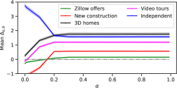
(a) Utility Maximization

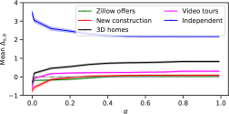
(b) Dollar Cost Per Unit Utility Minimization

Figure 1. Fair coverage of stakeholders

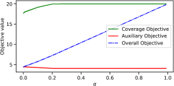
(a) Utility Maximization

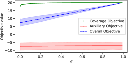
(b) Dollar Cost Per Unit Utility Minimization

Figure 2. Trade-offs between coverage and auxiliary objectives

Specifically, if we represent the proportion of recommended listings belonging to stakeholder $s$ by $\eta_{s,b}$ and the fair coverage threshold for the same stakeholder by $\delta_{s,b}$ as described in Section 3.1.1, then we plot the difference $\Delta_{s,b}=\lceil k(\eta_{s,b}-\delta_{s,b})\rceil$ averaged over all the buyers, for varying values of the parameter $\alpha$. When $\Delta_{s,b}\geq 0$ for all stakeholders, we conclude that fair coverage is achieved. On the other hand, $\Delta_{s,b}<0$ implies that at least one stakeholder $s$ is under represented in the $k$ recommendations. In Figure 1, we observe that a fair coverage of all stakeholder is achieved for both the auxiliary objectives, as the value of $\alpha$ i.e., importance of coverage objective increases.

5.2.2. Performance trade-offs:

Here, we visualize the trade-off between the primary fair coverage objective and the auxiliary objective during utility maximization and cost minimization in Figure 2. For clarity of visualization, we scale the auxiliary objective during cost per unit utility minimization by multiplying it with $10^{-6}$. We clearly see the trade-off between the coverage objective and the utility of recommendations in Figure 2a. When $\alpha=0$, only the highest utility listings are recommended. As the value of $\alpha$ increases, the overall utility of recommended listings is slightly sacrificed in order to improve the stakeholder coverage. During the cost per unit utility minimization in Figure 2b, the increase in cost of recommendations in order to improve the stakeholder coverage is not very apparent in this data due to the use of Stochastic Greedy algorithm with error parameter $\epsilon=0.1$.

5.2.3. Runtime comparisons:

Lastly, we compare the algorithm runtimes per buyer for different objectives in Figure 3. While the worst case time complexity for Lazy Greedy algorithm is same as that of Greedy algorithm, we observe that it is significantly faster in practice. In case of minimization auxiliary objectives, the Stochastic Distorted Greedy algorithm with error parameter $\epsilon=0.1$ is more efficient than the deterministic Distorted Greedy algorithm. Availability of such fast algorithms allows us to use this formulation of fair multi-stakeholder coverage in real-time personalized recommender systems.

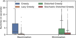
Figure 3. Runtime comparison for auxiliary objectives

6. Conclusion

In this work, we study the problem of fair multi-stakeholder recommendations. Our work confirms the idea that formulating multi-stakeholder coverage objective in form of a submodular function allows us to leverage existing submodular optimization techniques that can incorporate commonly used secondary objectives in personalized recommender systems. Using data from an online real-estate marketplace, we empirically evaluated the efficiency and scalability of our proposed approach. Incorporating non-linear secondary objectives such as learning-to-rank metrics into this framework remains an open research problem.

References

- (1)
- Abdollahpouri et al. (2017) Himan Abdollahpouri, Robin Burke, and Bamshad Mobasher. 2017. Recommender Systems as Multistakeholder Environments. In Proceedings of the 25th Conference on User Modeling, Adaptation and Personalization (UMAP ’17). ACM, New York, NY, USA, 347–348. https://doi.org/10.1145/3079628.3079657
- Avdiukhin et al. (2019) Dmitrii Avdiukhin, Grigory Yaroslavtsev, and Samson Zhou. 2019. ”Bring Your Own Greedy”+Max: Near-Optimal -Approximations for Submodular Knapsack. (Oct. 2019). arXiv:1910.05646 [cs.DS]
- Burke et al. (2016) R D Burke, H Abdollahpouri, and others. 2016. Towards Multi-Stakeholder Utility Evaluation of Recommender Systems. UMAP (Extended) (2016).
- Ekstrand et al. (2018) Michael D Ekstrand, Mucun Tian, Mohammed R Imran Kazi, Hoda Mehrpouyan, and Daniel Kluver. 2018. Exploring author gender in book rating and recommendation. In Proceedings of the 12th ACM conference on recommender systems. 242–250.
- Feldman (2018) Moran Feldman. 2018. Guess Free Maximization of Submodular and Linear Sums. (Oct. 2018). arXiv:1810.03813 [cs.DS]
- Filmus and Ward (2012) Yuval Filmus and Justin Ward. 2012. Monotone Submodular Maximization over a Matroid via Non-Oblivious Local Search. (April 2012). arXiv:1204.4526 [cs.DS]
- Guy (2015) Ido Guy. 2015. Social Recommender Systems. In Recommender Systems Handbook, Francesco Ricci, Lior Rokach, and Bracha Shapira (Eds.). Springer US, Boston, MA, 511–543. https://doi.org/10.1007/978-1-4899-7637-6_15
- Harshaw et al. (2019) Christopher Harshaw, Moran Feldman, Justin Ward, and Amin Karbasi. 2019. Submodular Maximization Beyond Non-negativity: Guarantees, Fast Algorithms, and Applications. (April 2019). arXiv:1904.09354 [cs.DS]
- Jannach and Adomavicius (2017) Dietmar Jannach and Gediminas Adomavicius. 2017. Price and Profit Awareness in Recommender Systems. (July 2017). arXiv:1707.08029 [cs.IR]
- Kamishima et al. (2018) Toshihiro Kamishima, Shotaro Akaho, Hideki Asoh, and Jun Sakuma. 2018. Recommendation independence. In Conference on Fairness, Accountability and Transparency. 187–201.
- Liu and Burke (2018) Weiwen Liu and Robin Burke. 2018. Personalizing fairness-aware re-ranking. arXiv preprint arXiv:1809.02921 (2018).
- Malthouse et al. (2019) Edward C Malthouse, Khadija Ali Vakeel, and Yasaman Kamyab Hessary. 2019. A Multistakeholder Recommender Systems Algorithm for Allocating Sponsored Recommendations. (2019).
- Mine et al. (2013) Tsunenori Mine, Tomoyuki Kakuta, and Akira Ono. 2013. Reciprocal Recommendation for Job Matching with Bidirectional Feedback. In Proceedings of the 2013 Second IIAI International Conference on Advanced Applied Informatics (IIAI-AAI ’13). IEEE Computer Society, USA, 39–44. https://doi.org/10.1109/IIAI-AAI.2013.91
- Modani et al. (2017) Natwar Modani, Deepali Jain, Ujjawal Soni, Gaurav Kumar Gupta, and Palak Agarwal. 2017. Fairness Aware Recommendations on Behance. In Advances in Knowledge Discovery and Data Mining. Springer International Publishing, 144–155. https://doi.org/10.1007/978-3-319-57529-2_12
- Pei et al. (2019) Changhua Pei, Xinru Yang, Qing Cui, Xiao Lin, Fei Sun, Peng Jiang, Wenwu Ou, and Yongfeng Zhang. 2019. Value-aware Recommendation based on Reinforcement Profit Maximization. https://doi.org/10.1145/3308558.3313404
- Sonboli and Burke (2019) Nasim Sonboli and Robin Burke. 2019. Localized fairness in recommender systems. In Adjunct Publication of the 27th Conference on User Modeling, Adaptation and Personalization. 295–300.
- Sürer et al. (2018) Özge Sürer, Robin Burke, and Edward C Malthouse. 2018. Multistakeholder recommendation with provider constraints. In Proceedings of the 12th ACM Conference on Recommender Systems. dl.acm.org, 54–62.
- Xia et al. (2015) P Xia, B Liu, Y Sun, and C Chen. 2015. Reciprocal recommendation system for online dating. 2015 IEEE/ACM International (2015).
- Yao and Huang (2017) Sirui Yao and Bert Huang. 2017. Beyond Parity: Fairness Objectives for Collaborative Filtering. In Advances in Neural Information Processing Systems 30. Curran Associates, Inc., 2921–2930.