The neutral hydrogen distribution in large-scale haloes from 21-cm intensity maps

Abstract

We detect the neutral hydrogen (HI) radial brightness temperature profile in large-scale haloes by stacking 48,430 galaxies selected from the 2dFGRS catalogue onto a set of 21-cm intensity maps obtained with the Parkes radio telescope, spanning a total area of $\sim$1,300 $\text{deg}^{2}$ on the sky and covering the redshift range $0.06\lesssim z\lesssim 0.10$. Maps are obtained by removing both 10 and 20 foreground modes in the principal component analysis. We perform the stack at the map level and extract the profile from a circularly symmetrised version of the halo emission. We detect the HI halo emission with the significance $12.5\sigma$ for the 10-mode and $13.5\sigma$ for the 20-mode removed maps at the profile peak. We jointly fit for the observed halo mass $M_{\rm v}$ and the normalisation $c_{0,\rm HI}$ for the HI concentration parameter against the reconstructed profiles, using functional forms for the HI halo abundance proposed in the literature. We find $\log_{10}{(M_{\rm v}/\text{M}_{\odot})}=16.1^{+0.1}_{-0.2}$, $c_{0,\rm HI}=3.5^{+0.7}_{-1.0}$ for the 10-mode and $\log_{10}{(M_{\rm v}/\text{M}_{\odot})}=16.5^{+0.1}_{-0.2}$, $c_{0,\rm HI}=5.3^{+1.1}_{-1.7}$ for the 20-mode removed maps. These estimates show the detection of the integrated contribution from multiple galaxies located inside very massive haloes. We also consider sub-samples of 13,979 central and 34,361 satellite 2dF galaxies separately, and obtain marginal differences suggesting satellite galaxies are HI-richer. This work shows for the first time the feasibility of testing theoretical models for the HI halo content directly on profiles extracted from 21-cm maps and opens future possibilities for exploiting upcoming HI intensity-mapping data.

1 Introduction

In the most widely accepted $\Lambda$CDM cosmological paradigm, the evolution of the Universe witnesses the formation of structures in a bottom-up scenario in which smaller overdensities grow and merge driven by gravitational instability (Peebles, 1980; Longair, 1998; Padmanabhan, 2002). This process determines the transition from an early homogeneous Universe to a highly structured distribution of matter known as the cosmic web, made of an assembly of large voids, walls, filaments and nodes. Therefore, the mapping and reconstruction of the cosmic web is an important benchmark to test cosmological models.

Our primary source of information for mapping the large-scale structure (LSS) of the Universe is provided by optical/IR galaxy catalogues, which during the past decades have undergone a dramatic improvement in terms of sensitivity and survey size. Among these, we can cite the the Two-degree Field Galaxy Redshift Survey  (Colless et al., 2001, 2dFGRS), the Six-degree Field Galaxy Survey (Jones et al., 2009), the WiggleZ Dark Energy Survey (Drinkwater et al., 2010) the Baryon Oscillation Spectroscopic Survey (BOSS Schlegel et al., 2009) and the Extended Baryon Oscillation Spectroscopic Survey (eBOSS Dawson et al., 2016). In parallel, progress has also been made in the cosmic web modelling with numerical simulations, which provide details on the large-scale distribution of baryons to levels beyond observational constraints (Cen & Ostriker, 1999; Davé et al., 1999; Cen & Ostriker, 2006; Haider et al., 2016; Cui et al., 2019). Results from numerical simulations are very efficient in probing the distribution of different baryonic phases. A detailed study of how baryonic components with different density and temperature are distributed across different cosmic web environments is described in Martizzi et al. (2019). These results show that the low-redshift diffuse baryonic gas in the LSS is expected to be mostly ionised. Consequently, new observational techniques, tailored to map the hot gas distribution, have been exploited to map cosmic web structures besides galactic surveys. X-ray observations, which probe the hottest baryonic components, are a relevant tool in this sense (Zappacosta et al., 2002; Eckert et al., 2015; Bregman et al., 2019; Walker et al., 2019; Vazza et al., 2019). Observations of the Sunyaev-Zel’dovich effect have also been largely exploited to study hot baryons in the cosmic web (Van Waerbeke et al., 2014; Hernández-Monteagudo et al., 2015; Ma et al., 2015; Génova-Santos et al., 2015; Tanimura et al., 2019; de Graaff et al., 2019).

In this effort of mapping baryons in the LSS it is interesting to consider the distribution of atomic hydrogen (HI) as the colder, neutral counterpart of the aforementioned probes. In the post-reionisation Universe the majority of intergalactic medium (IGM) is ionised, and almost all of the HI is believed to reside in dense clumps with column densities $\gtrsim 10^{20}\text{cm}^{-2}$, which are self-shielded against the ionising ultra-violet (UV) background, referred to as Damped Lyman-alpha sytems (DLAs, Wolfe et al., 2005; Prochaska & Wolfe, 2009). DLAs are expected to trace the large-scale distribution of galaxies; the corresponding cross-correlation was measured, for example, in Font-Ribera et al. (2012). Results from numerical simulations also prove that neutral hydrogen effectively traces the cosmic web at low redshift (Popping et al., 2009; Duffy et al., 2012; Cunnama et al., 2014; Takeuchi et al., 2014; Horii et al., 2017). Mapping the large-scale neutral hydrogen distribution is therefore important not only for the reconstruction of the underlying cosmic web, but also to achieve a more complete characterisation of the different baryonic phases across cosmic structures. Perhaps the most interesting targets in this sense are the nodes of the cosmic web, i.e. massive dark matter haloes, where the interplay between atomic and molecular hydrogen phases is a key element in processes of galaxy formation and evolution (Fu et al., 2010; Calette et al., 2018).

The total amount of HI in haloes hosting galaxy groups was investigated in Guo et al. (2020), where it was found to increase with the halo mass. The study separated the contribution of central and satellite galaxies, showing that the latter contribute for the majority of HI in haloes with masses above $\sim 10^{12}\,h^{-1}\text{M}_{\odot}$. Such mass represents the scale at which the HI content in central galaxies starts to be strongly suppressed by the feedback from active galactic nuclei (Di Matteo et al., 2005), as already proposed by previous studies (Kim et al., 2011, 2017; Zoldan et al., 2017; Baugh et al., 2019). Another conclusion is that the total HI content of a halo does not depend exclusively on its mass, but also on its richness and formation history (Guo et al., 2017). Such a dependence is however less relevant for very massive haloes (above $\sim 10^{13}\,h^{-1}\text{M}_{\odot}$) which are most likely assembled by mergers (Genel et al., 2010).

These considerations highlight the importance of a proper characterisation of the abundance and distribution of HI in dark matter haloes. This subject has been the focus of several studies that adopt HI-oriented halo models and provide functional parametrisations for describing the HI halo content, fitted over numerical simulations (Bagla et al., 2010; Villaescusa-Navarro et al., 2014, 2018) or observational data, most commonly DLA-related quantities (Barnes & Haehnelt, 2010, 2014; Padmanabhan & Refregier, 2017; Padmanabhan & Kulkarni, 2017). Although numerical simulations can give valuable hints on this subject, ultimately the proposed models need to be tested and verified against observations. Nonetheless, a universally accepted recipe to estimate the amount of HI residing in haloes of known mass, and its related spatial distribution, is still lacking. It is then worth considering how existing data can be used in new ways to provide alternative constraints.

A promising new probe for neutral gas in haloes is the 21-cm line emission due to the hyperfine-split transition in the ground state of neutral hydrogen (Pritchard & Loeb, 2008). This signal can be conveniently observed with ground-based facilities, and is therefore particularly useful at low redshift, where the Lyman-alpha line enters the ultra-violet range hindering observations of HI absorption. Radio 21-cm line observations can be used to detect HI-rich galaxies in large sky surveys. Among the resultant catalogues, we can cite the HI Parkes All Sky Survey (HIPASS, Meyer et al., 2004; Zwaan et al., 2005) extending up to $z\sim 0.04$ and the Arecibo Legacy Fast ALFA (ALFALFA, Martin et al., 2010; Hoppmann et al., 2015; Haynes et al., 2018) extending up to $z\sim 0.06$. HI sky surveys, however, become increasingly difficult at higher redshifts, as the faintness of the 21-cm emission requires long integration times, or reverting to stacking the spectra of galaxies (Delhaize et al., 2013; Rhee et al., 2013; Rhee et al., 2018). An alternative approach is provided by the intensity mapping technique, which allows spanning large sky areas in 21-cm with low resolution to map out the integrated HI emission on large scales, foregoing the detection of individual objects. This type of surveys can be quickly carried out with ground-based facilities and by tuning the central frequency of receivers it is possible to probe the emitting gas at different redshifts, resulting in a tomography of HI in the Universe which is ideal for reconstructing the three-dimensional cosmic web. The feasibility of tracing cosmic structures using 21-cm maps was first shown by Pen et al. (2009), by measuring the cross-correlation between the HIPASS maps and the 6dFGRS catalogue. Subsequent works continued on this line of exploiting the correlation between 21-cm maps and galaxy catalogues (under the assumption of full correlation between HI fluctuations and galaxy overdensities at large scales), to provide constraints on the cosmic HI density and bias parameters. Chang et al. (2010) combined 21-cm maps obtained with the Green Bank Telescope (GBT) with the DEEP2 survey catalogue (Davis et al., 2001), while Masui et al. (2013) combined GBT maps with the WiggleZ galaxy catalogue. Particularly relevant for the current work is the study described in Anderson et al. (2018), where the 21-cm maps are the result of observations performed with the Parkes radio telescope over the region spanned by the 2dFGRS catalogue. The main difference with respect to previous works is the much larger sky coverage, around 1300 deg².

A different strategy has been explored in Tramonte et al. (2019, hereafter T19), where the same combination of Parkes maps and 2dF galaxies has been employed to search for the HI emission of filamentary structures in the cosmic web. The signal was searched for directly at the map level, by coherently stacking the contribution from the region in between selected pairs of 2dF galaxies. The results set upper limits on the expected amount of HI in large-scale filaments, and for the first time showed the feasibility of this type of search directly on 21-cm maps. In this work, we want to conduct a similar analysis, but focussing this time on the HI found within haloes. Once again, the 2dF galaxies are used to trace the location of the cosmic web nodes, and, by taking advantage of the large sky coverage of these maps, a blind stacking technique is employed to enhance the halo signal over the background. The first, main goal of this work is to detect the halo 21-cm emission and to measure the associated HI radial profile. Secondly, we want to choose suitable functional forms discussed in the literature, describing the HI abundance in haloes, and test their prediction on our measurements. This procedure will allow us to fit for the mean mass of the objects we are detecting and for the concentration of the HI gas. For the first time, models are tested directly on profiles reconstructed from 21-cm maps.

We stress that the resolution of the available 21-cm intensity maps does not allow to resolve galactic-scale haloes in our study. This work targets instead the large-scale massive haloes in the cosmic web, at the scale of galaxy clusters and above ($M\gtrsim 10^{13}\,\text{M}_{\odot}$). In this context the 2dF objects serve as tracers of the underlying large-scale cosmic web, assuming full correlation between HI fluctuations and galaxy overdensity as in the aforementioned cross-correlation studies. Any detectable continuous radial HI emission at these scales is not to be ascribed to a diffuse neutral component in the IGM, which is highly ionised, but rather to the integrated contribution of the HI hosted in the halo member galaxies. Nonetheless, the very methodology described in this work can be applied to characterise the HI amount and distribution in galactic-scale haloes, provided intensity maps with the required resolution are available. It represents therefore a promising tool to analyse the next generation of HI survey data.

This paper is organised as follows. The description of the data set we employ is presented in Section 2. The methodology adopted for processing the 21-cm maps, and the corresponding results, are presented in Section 3 and further discussed in Section 4. The theoretical model we employ for computing the HI halo profiles is detailed in Section 5; in Section 6 we describe instead the corresponding parameter estimation. Finally, Section 7 lists the conclusions. Throughout this paper we adopt a flat-$\Lambda$CDM cosmological model with $\Omega_{\rm m}=0.3$, $\Omega_{\rm b}=0.049$ and $H_{0}=70\,\text{km}\,\text{s}^{-1}\text{Mpc}^{-1}$.

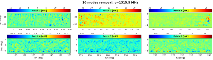
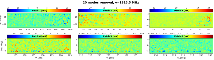
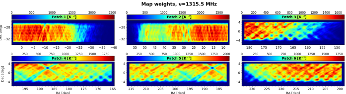
Figure 1: Top: Parkes 21-cm intensity maps of all six patches for the 10-mode removal case, sliced at the Multibeam Receiver central observing frequency and plotted in mK units in (RA, Dec) coordinates. Middle: same as in the top panel, but for the 20-mode foreground removal case. Bottom: Parkes weight maps for the same frequency slice, plotted in $\textrm{K}^{-2}$ units. The crossed stripes result from different telescope raster scans at constant elevation; the locations where bright radio sources have been masked are also visible as dark spots.

Table 1: Table summarising the main properties of the data set used in this work. For each Parkes patch we quote its central position and resolution (pixel size) in right ascension (RA, 486 pixels), declination (Dec, 106 pixels) and frequency ($\nu$, 64 pixels). The number of pixels in the three axes is the same for all patches. The RA pixel size in the low declination patches is larger because it is measured in degrees of polar rotation. Finally, the table reports the total number of 2dFGRS galaxies located within each patch, for the three different galaxy samples employed in this work.

Patch		RA [deg]			Dec [deg]			$\nu$ [MHz]			$N_{\rm gal}$	$N_{\rm gal}$	$N_{\rm gal}$
		Centre	Pixel size		Centre	Pixel size		Centre	Pixel size		[Full]	[Central]	[Satellite]
1		-18.0	0.092		-29.75	0.080		1315.5	1.0		7343	2209	5134
2		33.0	0.092		-29.75	0.080		1315.5	1.0		7708	2438	5270
3		165.0	0.080		-0.05	0.080		1315.5	1.0		9394	2658	6736
4		182.0	0.080		-0.05	0.080		1315.5	1.0		9960	2688	7272
5		199.0	0.080		-0.05	0.080		1315.5	1.0		9625	2542	7083
6		216.0	0.080		-0.05	0.080		1315.5	1.0		4310	1444	2866
Total											48430	13979	34361

2 Data set

The analysis addressed in this work requires the combined use of a galaxy catalogue, complete with angular and redshift information, and of foreground cleaned 21-cm maps, structured as three-dimensional data cubes. Clearly, the angular coverage and redshift span of these two data sets must have a significant overlap, in order to allow the association of the objects we are targeting with their HI emission. The choice for this work consists of 21-cm maps from the Parkes radio telescope over the 2dF galaxy catalogue region. This very data set was also employed in T19 and proved very efficient in the search for HI signal in intergalactic filaments. We review it in the following.

2.1 21-cm maps

The maps used in this work are the result of observations conducted using the Parkes radio telescope, equipped with the 21-cm Multibeam Receiver (Staveley-Smith et al., 1996), during a single week between April and May 2014; these observations specifically covered the volume spanned by the 2dF galaxy catalogue. In total, 152 hours of survey were conducted with the Multibeam Correlator, with a central observing frequency of 1315.5 GHz and a 64 MHz full bandwidth split into 1024 frequency channels with a 62.5 kHz resolution each. However, the frequency resolution was subsequently degraded to $1\,\text{MHz}$ after removing local radio frequency interference. The corresponding redshift range for the 21-cm emission spanned by the map is $0.06\lesssim z\lesssim 0.10$. The total sky coverage is approximately 1,300 square degrees, divided into a northern-galactic and a southern-galactic stripe. The map resolution is set by the Parkes beam, with a 14’ full width at half maximum (FWHM).

The full processing of the Multibeam Receiver data to yield the final 21-cm maps is detailed in Anderson et al. (2018). In order to improve the efficiency of the map-making code, the northern stripe was split into four different patches, and the southern one into two. These patches, although partially overlapping, underwent bandpass calibration and foreground removal independently. The current study takes it into account by initially performing separate analysis on different patches (see Section 3.1). Table 1 summarises the location, size and pixel resolution for all the patches, in both the angular and frequency space.

One of the most critical steps in yielding the final HI maps is the removal of the other radio foregrounds entering this frequency range, particularly Galactic synchrotron, that are 2 to 3 orders of magnitude higher than the underlying HI signal. By taking advantage of the smooth spectral distribution of the foregrounds, compared to the clumpy nature of the HI emission (Liu & Tegmark, 2012), the cleaning is done with a principal component analysis (PCA) which discards modes with higher frequency correlation (Switzer et al., 2015). Although the first modes are expected to be dominated by foregrounds, they still carry a marginal HI signal. As a result, a higher number of removed modes yields cleaner maps but produces also a higher loss of the targeted signal. The work in Anderson et al. (2018) established the 10-mode removal case as the optimal choice. In the current work we will use both the 10- and 20-mode removed maps to assess the effect of the foreground removal on our results. The same strategy, indeed, was adopted in T19 and showed some difference between the two cases when considering individual patches.

The 10 and 20-mode removed maps are therefore the starting point of our analysis, and are shown in Fig. 1 sliced at the central observational frequency; the value stored in each pixel is the observed HI brightness temperature. The same figure also shows the corresponding weight maps, which are necessary to account for the inhomogeneous sky coverage resulting from the telescope azimuthal drift scans. Each pixel stores the inverse squared noise weight, which is roughly proportional to the observing time with pointings within that pixel.

2.2 Galaxy catalogue

We employ the galaxy catalogue from the 2dF Galaxy Redshift Survey (Colless et al., 2001), which was carried out with the Anglo-Australian Observatory 3.9-meter telescope over the years 1997 to 2002. The majority of the objects targeted by the 2dF spectroscopic observations lie in the fields covered by the Parkes HI maps. The spectroscopic catalogue, which is publicly available, provides spectroscopic redshift information for 245,591 objects, and has to be appropriately queried to extract the most suitable galactic targets for our analysis.

First of all, we consider only sources with a reliable positive redshift estimate (according to a specific quality flag in the data), lowering the total number of sources to 227,190. At this point, we split the catalogue into six sub-catalogues contained in the 21-cm map patches. We discard sources located within $1\,\text{deg}$ in declination and $3\,\text{deg}$ in right ascension from the Parkes patch edges (patches are indeed more extended in right ascension than in declination by a factor $\sim 3$) as these regions are more likely affected by strong residual contaminations. For the same reason we excise all sources whose redshift falls within the lowest 10 MHz or the highest 4 MHz in the frequency range covered by Parkes, following the criterion adopted by Anderson et al. (2018). Notice that if a galaxy falls in the intersection area of two patches, it is included into both of the corresponding sub-catalogues. This query reduces the total galaxy number to 48,430 objects, counting the repetitions in neighbouring patches. Hereafter we shall refer to this selected ensemble of galaxies as the full 2dF galaxy sample.

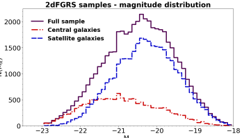
Figure 2: R-band absolute magnitude distribution, computed over bins with size 0.1, for the three samples of galaxies considered in this work. These three samples are the full 2dF galaxy sample bounded by the Parkes data volume, the selected locally brighter galaxies (the central galaxy sample) and the complementary sample between the two, made by satellite galaxies.

The selected galaxies serve to identify the position on the maps of their hosting dark matter haloes, whose HI radial profile is the object of the present study. It is clear that the 2dF sample selected with the procedure we just described contains galaxies with different masses and morphological types, and belonging to different environments in the cosmic web. Although the results of our analysis are mostly insensitive to the properties of individual galaxies, we can still apply a further selection by exploiting their magnitude information, following the criterion adopted in T19. In that case, the galaxy catalogue served to locate the endpoints of large-scale filaments, corresponding to massive haloes likely hosting galaxy clusters. The 2dF catalogue was then queried to extract the locally brighter galaxies, that are the most likely to be located in the centres of those haloes. We shall repeat the same selection here, and consider a galaxy “central” if no brighter galaxy is found within a projected separation of $1.0\,h^{-1}\text{Mpc}$ and a line-of-sight (LoS) separation of $|c\Delta z|=1000\,\text{km}\,\text{s}^{-1}$ (this isolation criteria was initially proposed in Planck Collaboration et al., 2013). We find in total 13,979 central galaxies. For the current work, however, it is also interesting to consider the complementary sample of 34,361 satellite galaxies. As a result, we are left with three galaxy samples that will be used for our study: the full 2dF sample, the one made by the central galaxies and the one made by the satellite galaxies. In Fig. 2 we show the magnitude distributions of these three 2dF sub-catalogues: as expected, the brighter, central galaxies have a distribution centred on lower values of the absolute magnitude, while the satellite galaxies are more numerous and fainter on average. Although it is not possible to study the profile for galaxies with similar magnitude, this strategy still provides a magnitude-based separation of the 2dF catalogue, which can be useful to assess the dependence of the halo HI content on the local galaxy environment. The way the full, the central and the satellite catalogues are distributed across the different patches is reported in Table 1.

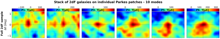
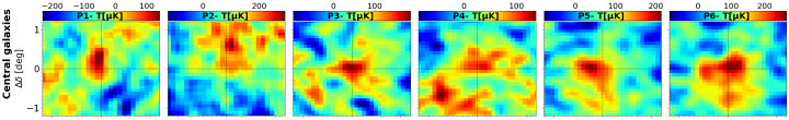
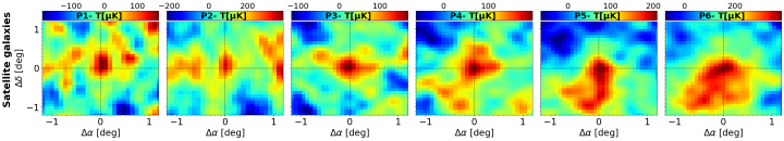
Figure 3: Results of the galaxy stacking procedure described in Section 3.1, shown separately for the six Parkes patches in the 10-mode removed maps case. Different rows show the results of stacking the full 2dF galaxy sample (top row), the central galaxy sample (middle row) and the satellite galaxy sample (bottom row).

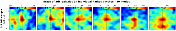
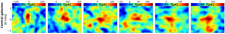
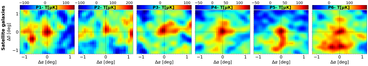
Figure 4: Same as in Fig. 3, but showing the stacks on the 20-mode removed maps.

3 HI profiles from intensity maps

In this section, we describe the methodology we employ to combine the Parkes HI maps and the 2dF galaxies for extracting the observed HI halo profile. The low resolution of intensity mapping does not allow the detection of individual galaxies at the map level, requiring further data processing to enhance the signal we are interested in. In our case, we revert to stacking the map area centred at the selected galaxy locations, taking advantage of the full statistics available for the three galaxy samples defined in Section 2.2. The HI profile is then extracted from the resultant stacked maps, after symmetrizing the signal around the halo centre. The uncertainty associated with this reconstructed profile is obtained with a bootstrap method by repeating the stacks on a set of randomized galaxy samples. Each of these steps is detailed in the following. A discussion of the results is instead provided in Section 4.

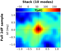
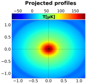
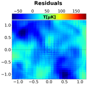
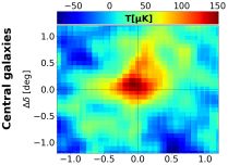
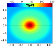
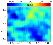
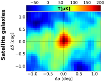
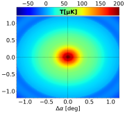
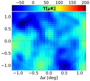
Figure 5: Results from the data analysis described in this section. Rows from top to bottom show, in order, the results from stacking the full selected 2dF galaxy sample, the subsample of locally brighter galaxies and the subsample of satellite galaxies. For each case, we show the final stack obtained combined the six Parkes patches (left column), the circular-symmetrised modelled emission obtained from the stack (central column) and the residual map obtained by subtracting the model from the stack (right column).

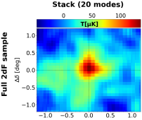
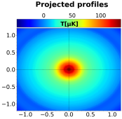
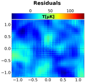
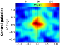
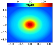
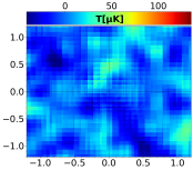
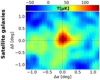
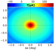
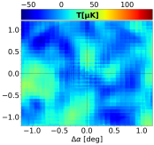
Figure 6: Same as in Fig. 5 but showing the results for the stacks on the 20-mode removed maps.

3.1 Galaxy stacking

Initially, we consider each of the six Parkes patches separately, in combination with the 2dF sub-sample overlapping with it. For each galaxy the 2dF catalogue reports its equatorial coordinates and its redshift; this information allows us to locate the galaxy in the corresponding three-dimensional Parkes HI patch. First of all, a two-dimensional HI map in (RA, Dec) is extracted by slicing the HI cube at the frequency corresponding to the galaxy redshift. From this slice, we then trim a sub-map centred on the galaxy position, with total extension $(2.4\times 2.4)\,\text{deg}^{2}$. For a generic galaxy $i$ located in the $j$th patch, we call $T_{i}^{(j)}$ the resultant sub-map, with $T$ standing for brightness temperature, which is the observable plotted in the maps. The same procedure is applied to the Parkes weight cubes, yielding a weight map $W_{i}^{(j)}$ for this particular galaxy and patch. Let $N_{j}$ be the total number of galaxies in the $j$th patch. The final stack map $T^{(j)}$ for this patch is then computed as:

$$T^{(j)}=\frac{1}{W^{(j)}}\sum_{i=1}^{N_{j}}T_{i}^{(j)}W_{i}^{(j)},$$ (1)

with $W^{(j)}$ the total weight:

$$W^{(j)}=\sum_{i=1}^{N_{j}}W_{i}^{(j)}.$$ (2)

The above procedure is applied to both the 10 and 20-mode removed maps and using all our three 2dF sub-samples. For every choice of the foreground removal and the galaxy sample, we end up with six stack maps, one for each patch. All these stacks are shown in Fig. 3 for the 10-mode removal case and in Fig. 4 for the 20-mode removal case. The stacking procedure described above does not imply any rotation of the field of view since it only produces a superposition of different regions extracted from the data cubes. Therefore, the final map axes retain the direction along the right ascension and declination axes of the Parkes maps, as it is made explicit in our plots. The stack axes values are quoted as angular separations $\Delta\alpha$ and $\Delta\delta$ from the centre, corresponding to the expected position of the stacked galaxies. We also comment that the original Parkes maps pixelisation is still visible in the stacks, corresponding to the pixel size of 0.08 deg (0.092 deg for the right ascension in patches 1 and 2) quoted in Table 1.

The stack results in individual Parkes patches provide a clear detection of the HI halo emission, although the region surrounding the central peak is often affected by spurious structures. We will discuss this issue more in detail in Section 4. For the moment it suffices to know that the (low) available statistics of the stacked galaxy samples is a major factor determining the appearance of a noisy background. To mitigate this effect, we choose to combine the contributions from all six patches together. Formally, this results in a final stack map $T_{\rm stack}$ defined as:

$$T_{\rm stack}=\frac{1}{W_{\rm stack}}\sum_{j=1}^{N_{\rm p}}T^{(j)}W^{(j)},$$ (3)

where $N_{\rm p}=6$ is the total number of available patches and

$$W_{\rm stack}=\sum_{j=1}^{N_{\rm p}}W^{(j)}$$ (4)

is the overall weight. Once again, this computation is repeated for the three 2dF sub-catalogues and for the two foreground removal schemes. The resultant stacks are shown in the first column of Fig. 5 for the 10-mode maps and in the first column of Fig. 6 for the 20-mode maps. The improvement of the available statistics is visible in these stacks, yielding more homogeneous backgrounds and more circularly symmetric halo peaks. We conclude that the quality of the individual patch stacks is too poor for any further analysis, and consider the overall stacks exclusively for the rest of this work.

This procedure merges together the contribution from haloes of different sizes, the final result being an average of the stacked sample. This effect could be mitigated by scaling each sub-map radial units by the corresponding halo virial radius. Neverthless, the latter is not know beforehand in the blind stack we are performing, and any indirect estimate would not be accurate enough to be used as a scaling unit. The change in apparent size with redshift could be taken care of by performing the stack in linear coordinates; this, however, would imply to lose information on the angular scale of the signal we are observing in relation to the Parkes beam extension. We therefore perform all the stacks in angular coordinates, being aware that the resulting halo emission is to be interpreted as an average measurement. This procedure preserves the beam dilution effect consistently and enables a final direct comparison of the recovered signal with the beam size, as it is detailed in Section 3.2.

3.2 Profile extraction

The final goal of our stacking analysis is to obtain the HI brightness temperature profile $T(\theta)$ for the large-scale haloes, expressed as a function of the observed angular separation $\theta$ from the halo centre. We do not make any assumption on the shape of such profile, and we extract it directly from the stack maps; the only condition we impose is that the halo profile is circularly symmetric. First, for each stack, we compute the average background temperature as the mean value of all pixels whose separation from the centre is higher than 1 degree. Because we are interested in the local excess temperature due to the HI emission, this background value is subtracted from the corresponding map. We then build a set of concentric annuli around the centre of each stack, corresponding to a set of bins in the angular separation from the centre of the halo. We choose a radial bin angular size of 0.015 deg, and for each annulus, we take the mean of the map pixel values found within its boundaries as the value of the HI brightness temperature profile at that radial separation.

Before considering the resultant profiles, we show the results of this methodology at the map level. The second column in Figs. 5 and 6 shows the modelled halo HI brightness maps for each of the foreground removal and 2dF sample cases, built by assigning to each circular annulus the average found as just described. These maps are two-dimensional projections of the reconstructed halo profile. Thus by construction, they represent a circularly symmetrised version of the stacks shown in the first column. To assess how well the reconstructed halo profiles capture the features in the original stacks, the last column in the same figures reports the residual maps obtained by subtracting the profile maps from the stacks. We see that the halo peak is consistently removed, the residuals being usually below $\sim 50\,\mu\text{K}$ and typically located far away from the halo centre.

The resultant radial profiles are plotted in different combinations in Figs. 7 and 8. In Fig. 7 we show, for each foreground removal case, the comparison of the profiles obtained stacking the three 2dF samples considered in this work. In Fig. 8, instead, we show for each individual 2dF sample the comparison between the profiles extracted from different foreground removed maps. In these figures, the profiles are superimposed to a shaded region which quantifies the profile 1-$\sigma$ uncertainty, computed following the procedure described in Section 3.3. In all of the panels, we show as well the radial profile for the Parkes beam, assumed for simplicity as perfectly Gaussian with $\theta_{\rm FWHM}=14^{\prime}$, with an amplitude arbitrarily set to the mean between the peaks of the profiles plotted in the same panel. In this context, the beam profile serves to prove that the halo HI emission is actually resolved in these observations, and it is then meaningful to proceed with a study of the reconstructed profile. The relationship between the profiles shown in Figs. 7 and 8 is discussed in Section 4.

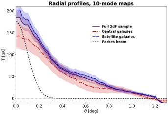
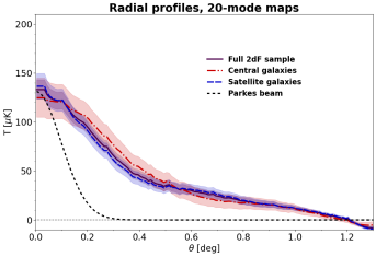
Figure 7: Radial profiles extracted from the stacks of the different galaxy samples used in this work showed for the case of the 10-mode removed maps (left panel) and the 20-mode removed maps (right panel). The shaded region around each profile shows the size of the error bar computed following the procedure described in section 3.3. For comparison, the 14’ FWHM Parkes beam is also plotted, normalised at its maximum to the mean of the profile amplitudes.

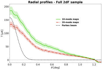
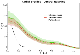
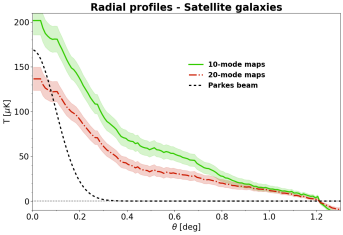
Figure 8: A complementary version of Fig. 7, in which the comparison is between profiles extracted from different foreground cleaned maps. From top to bottom, we show such a comparison for the full 2dF sample, the central galaxy sample and the satellite galaxy sample.

Table 2: Peak brightness temperature value and uncertainty for the profiles extracted using different foreground removal maps and 2dF samples. The corresponding detection significance is also quoted for each case.

	10-modes	20-modes
Full 2dF sample	$T=(184.5\pm 14.7)\,\mu\text{K}$	$T=(133.1\pm 9.9)\,\mu\text{K}$
	$(12.5\sigma)$	$(13.5\sigma)$
Central galaxies	$T=(142.3\pm 28.1)\,\mu\text{K}$	$T=(124.7\pm 20.0)\,\mu\text{K}$
	$(5.1\sigma)$	$(6.2\sigma)$
Satellite galaxies	$T=(201.7\pm 16.1)\,\mu\text{K}$	$T=(136.5\pm 13.0)\,\mu\text{K}$
	$(12.5\sigma)$	$(10.5\sigma)$

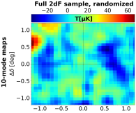
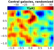
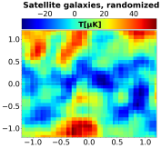
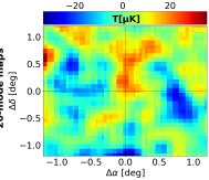
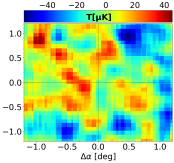
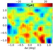
Figure 9: Example of one realisation of the randomised catalogue stacks. Columns from left to right show, in order, the results from stacking the randomised full galaxy sample, the randomised central galaxy sample, and the randomised satellite galaxy sample on the 10-mode (top row) and 20-mode (bottom row) removed maps. The top and bottom row stacks should be compared with the left column of Figs. 5 and 6 respectively, and show the absence of the signal peak.

3.3 Error estimation

The uncertainties on the extracted profiles are derived using a bootstrap approach, consisting of repeating the method described so far on a set of randomised galaxy catalogues. More precisely, for each of the three 2dF sub-samples, we generate 500 replicas in which the equatorial coordinates of each galaxy are randomly chosen within the ranges allowed by the corresponding Parkes patch; the galactic redshift values, instead, are left unchanged. For each of these scrambled catalogues we repeat the same stacking procedure we described in Section 3.1. In Fig. 9 we show what the final stacks look like in one realisation chosen out of the total 500, again for both the 10 and 20-mode removal cases, and using the randomised versions of all three 2dF sub-samples. For simplicity, we show already the overall stacks obtained by combining the six Parkes patches, but the stacks are initially performed on individual patches in the same way as for the real catalogues.

Although in this case there is no visible halo peak, we follow the same procedure described in Section 3.2, and extract the map profile over the same set of radial bins. As a result, for each foreground removal and each sub-catalogue choice, we obtain a set of 500 random profiles. For each bin, the dispersion of the measured brightness temperature across the 500 realisations yields and estimate of the error associated to the real profile value in that bin. If we denote by $T^{(k)}(\theta)$ the HI brightness temperature profile from the $k$th realisation, as a function of the angular separation $\theta$ from the halo centre, and

$$\overline{T}(\theta)=\frac{1}{N_{\rm r}}\sum_{k=1}^{N_{\rm r}}T^{(k)}(\theta)$$ (5)

is the mean randomised profile (with $N_{\rm r}=500$ the total number of realisations), then the variance for the randomised realisations is computed as:

$$\sigma^{2}_{\rm T}(\theta)=\frac{1}{N_{\rm r}}\sum_{k=1}^{N_{\rm r}}\left(T^{(k)}(\theta)-\overline{T}(\theta)\right)^{2}.$$ (6)

The quantity $\sigma_{\rm T}(\theta)$ represents the uncertainty associated to the real data profile as a function of the angular separation $\theta$, and is plotted as a shaded region around the observed profiles in Figs. 7 and 8. In table 2 we report for all profiles the peak temperature value with its uncertainty. The ratio between the two, also reported in the table, quantifies the significance of the detection.

The bin-dependent uncertainty computed with Eq. (6) does not complete the statistical characterisation of the observed profiles. Indeed, we remind that in this case different bins are not statistically independent. A single halo profile covers an extended range of angular separations, thus introducing a correlation between pairs of $\theta$-bins (which becomes more important the closer the bins are). The proper object to summarise this correlation is the covariance matrix. The covariance $\mathcal{C}_{\rm T}(\theta_{i},\theta_{j})$ between the angular separation bins centred at $\theta_{i}$ and $\theta_{j}$ is computed as:

$$\mathcal{C}_{\rm T}(\theta_{i},\theta_{j}) = \frac{1}{N_{\rm r}}\sum_{k=1}^{N_{\rm r}}\left(T^{(k)}(\theta_{i})-\overline{T}(\theta_{j})\right)$$ (7)

$$\times \left(T^{(k)}(\theta_{j})-\overline{T}(\theta_{j})\right),$$

where this time we made the discretised nature of the angular variable $\theta$ explicit. The individual bin variance computed with Eq. (6) corresponds to the covariance matrix diagonal, in the particular case of setting $\theta_{i}=\theta_{j}$ in Eq. (7). The resultant covariance matrices are plotted in Fig. 10 for the six combinations of maps and samples, and will be used in section 6 for the parameter estimation.

4 Discussion of data analysis results

We dedicate this section to a discussion of the results obtained so far with the joint analysis of the Parkes maps and the 2dF galaxy sample.

The stacks in Figs. 3 and 4 show a clear detection of a 21-cm signal peaked in the map centre at a level of 100 to 300 $\mu\text{K}$, with the 10-mode stacks having a systematically higher peak value than the 20-mode stacks. These stacks are showing the merged contribution of the 21-cm emission from the bulk HI contained in the haloes hosting the galaxies we are targeting. However, the background signal surrounding the central halo is not homogeneous and shows several structures, in some cases with an amplitude comparable to the central halo signal. This phenomenon is most likely due to a combination of the limited samples statistics and the contribution from residual foregrounds. Indeed, the usage of the full 2dF sample, which has the highest statistics, seems to mitigate this effect slightly. However, if we look again at the last three columns of Table 1, it is clear that the number of stacked galaxies alone is not enough to account for these structures. Patch number 4 seems to be the most heavily affected, although it is the patch with the highest number of galaxies. This situation suggests that foreground residuals are also contributing to this effect. In this sense, it is essential to compare their amplitude with the amplitude scale of the 21-cm maps we employed. By looking back at Fig. 1, we see that the original Parkes maps have typical fluctuations at the level of $\sim 10\,\text{mK}$. Our final stacks allow us to identify structures at the level of $\sim 100\,\mu\text{K}$ which is two orders of magnitude lower. Any spurious signal initially present in the maps, such as thermal noise or foreground residuals, would also enter the final stacks, and its relative importance compared to the actual signal is determined by the available statistics. As commented in Section 2.1, different patches underwent foreground removal independently, and it is possible for some patches to be more affected than others in this sense. Another fact corroborating this hypothesis is that the stacks on the 20-mode maps, which have undergone a more thorough foreground removal, are overall less affected by background structures. The only exception is patch number 6, where, although the asymmetrical structures are observed in both foreground removal cases, the 20-mode maps look worse. We have to take into account that the observed fluctuations may also proceed from actual HI emission distributed off-centre with respect to the selected central position for our stacking. If this is the case, then, using a different 2dF sub-sample should make a difference. In fact, for patch 6, the central galaxy catalogue and the satellite galaxy catalogue provide the best and worst results respectively (with the full 2dF catalogue in between), thus supporting the idea that the selected central 2dF galaxies are more HI-rich. Unfortunately, this conclusion cannot be generalised because it does not hold for all the six patches (for example, in patches 2 and 4, we observe the opposite situation).

To summarise, we can list three main properties emerging from the stacks at the individual patch level. First, the comparison between the 10 and 20-mode removal cases shows that the 20-mode removal maps provide cleaner stacks (with the only exception of patch 6). Second, for the same removal case, neither the central nor the satellite galaxy samples seem to provide consistently a better galaxy selection than the full 2dF sample, which is probably favoured by its higher statistics. Third, for the same removal case and chosen sub-sample, there is not a clear trend in the quality of the resultant stacks across patches, nor a clear dependence of the observed peak and fluctuation amplitudes on the number of galaxies available for a particular patch. That said, it is clear that the limited statistics of our sample is a crucial factor in this type of analysis. Even the choice of the full 2dF catalogue does not provide a statistically large enough sample to allow the study of an HI halo profile in individual patches. For this reason, we shall combine the contribution from the six patches and study the stack of each of the three 2dF sub-samples as a whole. Although the stacks may look better in some particular patches, we have no a priori reason to discard the other ones, so the contribution from all six patches is considered in their combination.

The resultant overall stacks shown in the first column of Figs. 5 and 6 show the improvement in the stack quality resulting from the larger stacked samples. Although the background fluctuations are still visible, their amplitude is no longer comparable with the peak value of the HI emission. These maps can now be used for the study of the halo profile. We notice that the central galaxy sample is now clearly the worst choice, as its final stacks still show a pronounced asymmetry, especially for the 10-mode case. This phenomenon may suggest that the location of the central galaxies does not match the loci of higher HI-density in the local Universe. Once again, the 20-mode maps yield better results than the 10-mode maps, as the resultant peaks tend to be more symmetric and the backgrounds slightly more homogeneous. In the same figures, the projected profile maps are not particularly meaningful; they provide a quick visual check that the HI profiles are representative of the stack maps they are extracted from. The associated residual maps show a consistent cancellation of the central HI peak. Their amplitude fluctuations measure to what extent the initial stack maps deviate from circular symmetry. In this case, a better result is achieved by the full 2dF sample. Indeed, it is expectable that a higher number of stacked galaxies would increase the signal-to-noise ratio of the HI emission and produce more rounded peaks.

Before analysing the radial profiles, it is worth commenting on the results of the bootstrap method employed for estimating the statistical uncertainties of the measured signal. The maps reported in Fig. 9 show what we obtain by stacking the randomised galaxy catalogues, for one particular realisation. Notice that it is still possible to compare stacks produced with the same sample across the two foreground removal cases, as the randomisation is the same. However, such a comparison is not very informative in this case. What is important here is to compare the final stacks with the ones obtained with the real data. In other words, the first and second rows of Fig. 9 should be compared with the first column of Figs. 5 and 6, respectively. We see that the randomisation destroys the detected halo signal, and the resultant stacks show absolutely no evidence of a central emission. In this case, we do not show the extracted halo profiles, which do not carry any useful information. However, the repetition of this procedure 500 times provides us with a set of profiles that we can use to characterise the statistical properties of the observed halo emission. The dispersion of these profiles for individual bins provides the 1-$\sigma$ uncertainties associated with the halo emission, visible in Figs. 7 and 8. We decided to quote explicitly the temperature and error for the peak of all profiles (Table 2) to quantify the significance associated with its measurement. The full 2dF sample, being the largest, clearly provides the highest significance, but even for the central sample the values are higher than 5, confirming the robustness of our detection. The correlation across pairs of bins can also be computed and is encoded in the covariance matrices plotted in Fig. 10. Although, as expected, the signal is peaked at the diagonal, we see that a significant area of the off-diagonal region has non-null covariance, meaning that the angular bins (particularly those closer to the peak) cannot be considered independent. This information is to be taken into account in the parameter estimation described in Section 6.

Finally, we discuss the resultant radial brightness temperature profiles shown in Figs. 7 and 8, which are the primary goal of our data analysis. First of all, as already mentioned above, the fact that all profiles are considerably more extended than the Parkes beam implies that the emission we are observing is resolved, and it is then meaningful to study its shape. If the signal radial extension were comparable with the beam Gaussian, we would just be observing the instrumental response to sources that are not resolved, and it would not be possible to test any theoretical model on it. The finite instrumental resolution still affects our detections, as the halo HI brightness temperature is convolved with the telescope beam. Ideally, a smaller beam would allow to map smaller scales and to obtain a higher fidelity reconstruction of the physical 21-cm emission. In this case, however, we are observing profiles extended out to $\sim 0.8\,\text{deg}$, and although the 14 arcminutes are still an essential fraction of the signal extension, they allow to resolve it and to map the decrease of the emission towards larger angular separations.

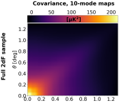
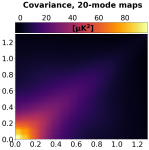
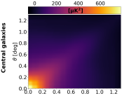
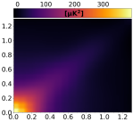
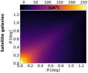
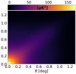
Figure 10: Covariance matrices obtained from the stacks of the 500 randomised catalogues. Rows from top to bottom show, in order, the results for the full, the central and the satellite galaxy samples, over the 10-mode (left) and 20-mode (right) removed maps. The correlation between neighbouring bins is evident, particularly for the lowest angular radii.

We focus now on the reconstructed halo profiles in Fig. 7, which allows a direct comparison of the different 2dF samples for a chosen foreground removal case. The most evident feature is that the full 2dF sample typically lies in between the central and the satellite samples. Stacking satellite galaxies results in a higher peak, and this may suggest that this type of galaxies is spatially associated with a higher abundance of HI compared to the central galaxies. As a result, when considering the full 2dF sample, the inclusion of central galaxies lowers the mean HI content, and consequently, the full sample profile has a lower peak amplitude than the satellite sample profile. Although the separation between centrals and satellites is not neat, as the contribution from one type can be picked up by the beam when centering the stack on the other, it still shows that different environments affect the galactic HI abundance, and such a difference can be detected with 21-cm intensity maps. This situation is more visible for the 10-mode removal case; the 20-mode maps, instead, yield remarkably consistent profiles across the different 2dF sub-samples. We can interpret this observation by stating that either the differences in the profiles for the 10-mode case are enhanced by a higher contamination of foreground removal, or that the 20-mode removal excises most of the physical HI emission, thus cancelling the differences coming from the choice of a different galaxy sample. Unfortunately, it is not possible to extract more information in this sense with the available data set. However, we have to stress that also for the 10-mode removal case we are talking about a separation between profiles which is still within 1-$\sigma$. The selection of a different galaxy sample determines only a marginal variation across different profiles. A final observation that can be extracted from these plots is that the profile obtained stacking the central galaxies is less concentrated than the one obtained by stacking the satellite galaxies. This effect was already visible in the final stack maps in the first column of Figs. 5 and 6, where the central galaxy stacks extended over a broader region. This could reinforce the hypothesis that the central galaxies do not trace locations with the higher abundance of HI in the volume spanned by the Parkes patches.

We conclude this section by considering the profiles plotted in Fig. 8, where the same 2dF sub-sample is shown for both foreground removal cases. As it was already clear from the stack maps, the 10-mode profile is always systematically higher than the 20-mode one. However, it is interesting to notice that the two profiles are not compatible when stacking the full or the satellite samples, while a much better consistency is achieved with the central 2dF sample. This situation is a result of the 10-mode profile being substantially lower for the central sample compared to the other ones. As already mentioned, it is likely that in this case there is an essential mismatch between the bulk of the 21-cm signal (whether it is actual halo HI emission or residual radio foreground) and the positions of the central galaxies, which has the effect of distributing the signal over a larger area, thus artificially broadening the profile and diluting its peak value.

5 Theoretical modelling

The last part of this work is dedicated to the theoretical prediction of the observed halo HI emission. Our goal is to provide a recipe to compute the mean expected radial brightness temperature profile for a generic halo of virial mass $M_{\rm v}$ at redshift $z$. This procedure will enable us to use the profiles extracted from the Parkes maps as a benchmark to test this theoretical model and to fit for the main parameters controlling the abundance and distribution of HI in haloes.

Things, in this case, are complicated by the fact that our stacks merge the contributions from halos with different masses and radial extensions. In this case, the formally most correct way to reproduce the observed profiles is to cross-correlate the galaxy sample and the HI signal. Such a strategy has been employed in Gong et al. (2019) and Tanimura et al. (2020) to model the observed profile of the thermal Sunyaev-Zel’dovich in galaxy clusters. In our case, however, we do not have prior information on the stacked halo mass distribution, which is a crucial quantity involved in this computation.

For this reason we limit this section to the computation of the expected profile observed for a single halo with chosen mass and redshift. This prediction will be compared to the observed profiles from Section 6, regarded as being produced by a single type of haloes whose properties are the mean of the corresponding stacked sample. Although this is an approximation, it is the best type of modelling we can provide for the current data set.

There are two main quantities required to predict the HI halo profile. The first is the HI mass to halo mass (HIHM) relation, which establishes the total HI mass to be assigned to a generic dark matter halo. The second is the choice of a suitable shape for the HI profile, which dictates how the HI is distributed inside its host halo. Different options have been explored in the literature. We discuss them in the following and justify our choices, before detailing the steps we took to theoretically predict the observed HI brightness temperature profile.

5.1 The HIHM relation

The relationship between the HI mass and the virial mass of a halo cannot be derived analytically. A universal recipe linking the halo mass to its HI content is still lacking, most likely a result of the observed scatter in this relation (Papastergis et al., 2013). Several functional forms have been proposed in the literature, justified by numerical simulation results or analytic approaches, with varying numbers of free parameters to be estimated by fit over observations.

The most straightforward way to model the HIHM is to take the HI mass as a fraction of the halo mass. Results from numerical simulations show that the HI fraction is expected to be maximum for halo masses of order $10^{11}\,\text{M}_{\odot}$, while disfavouring the assignment of HI to much lower or higher masses (Pontzen et al., 2008). Taking this information into account, Bagla et al. (2010) proposed a constant fraction for the HI mass within a bounded range, while Barnes & Haehnelt (2010) and Barnes & Haehnelt (2014) adopted a proportionality relation between the HI mass and the halo mass with a cut-off term for low halo masses. This functional form was further explored in Villaescusa-Navarro et al. (2014) and Padmanabhan & Refregier (2017), the latter reference also including a high-mass cut-off and including the dependence on the virial halo mass with a generic power. The cut-offs are usually expressed in terms of the virial halo velocity. The resultant relations are expressed in a parametric form, leaving the cut-off velocities, the overall normalisation and possibly the logarithmic relation slope as free parameters.

A different approach is proposed in Padmanabhan & Kulkarni (2017), where the HIHM relation is built on the basis of the observed HI mass function (HIMF) via abundance matching. This technique consists in matching the cumulative abundance of dark matter halos with the corresponding abundance of HI galaxies. The former is obtained by integrating the halo mass function, for which they chose the parametrisation from Sheth & Tormen (2002). The latter is obtained by integrating the HIMF, for which they employed a combination of the HIMFs fitted on the HIPASS and ALFALFA catalogues using a Schechter functional form. The relationship between the HI mass and the halo mass is implicitly contained in this matching, which the authors solved in the range $10^{6}\,\text{M}_{\odot}<M_{\rm HI}<10^{11}\,\text{M}_{\odot}$ (this being the range allowed by the HI surveys results). The resultant HIHM shows that the HI mass increases over the full range as a function of the halo mass. However, the growth is slower for masses above $M_{\rm HI}\sim 4\times 10^{11}\,\text{M}_{\odot}$. This behaviour is better shown in terms of the HI to halo mass fraction, which reaches a peak of $\sim 1$% in correspondence to the turning point, and decreases for lower or higher masses. On average, its value is around $10^{-3}$, showing that this relation can be applied for haloes of masses between $10^{9}\,\text{M}_{\odot}$ and $10^{14}\,\text{M}_{\odot}$. The authors fitted the HIHM with the following functional form

$$M_{\rm HI}=2N_{10}M_{\rm v}\left[\left(\dfrac{M_{\rm v}}{M_{10}}\right)^{-b_{10}}+\left(\dfrac{M_{\rm v}}{M_{10}}\right)^{y_{10}}\right]^{-1},$$ (8)

where $N_{10}$, $M_{10}$, $b_{10}$ and $y_{10}$ are model-dependent parameters whose best-fit values are

$$N_{10} = (9.89\pm 4.89)\times 10^{-3},$$

$$M_{10} = (4.58\pm 0.19)\times 10^{11}{\rm M}_{\odot},$$

$$b_{10} = 0.90\pm 0.39$$

$$y_{10} = 0.74\pm 0.03,$$ (9)

as reported in the reference. As it was remarked by the authors, it is interesting to remind that this behaviour reminds closely the stellar mass to halo mass (SHM) relation. In fact, the functional form Eq. (8) had been originally introduced in Moster et al. (2010) and later employed by Moster et al. (2013) to fit for the SHM relation, again built via abundance matching. This similarity stresses the strict connection between HI gas and star-forming gas in the galactic baryon cycle.

In this work we are going to use the functional form from Eq. (8) with the parameters quoted in Eq. (5.1) as the recipe for computing the HIHM. The reason is twofold. First of all, the stronghold of the abundance matching method is that the HIHM is built directly based on observational data, and as such is to some extent less affected by the assumptions implied by other parametrisations. The only assumption required in this case is that there is a monotonic relation between the HI mass and the halo mass and that one dark matter halo hosts one and one only HI-selected galaxy. Secondly, this fitting function has been built for the local Universe, which is also the target of our study: the HIPASS survey covers redshift values below $z\sim 0.04$, while the ALFALFA survey below $z\sim 0.06$. Our galaxy sample spans the redshift range from 0.06 to 0.1; to a first approximation, we can, therefore, extrapolate the results from HIPASS and ALFALFA over our redshift range. The analysis in Padmanabhan & Kulkarni (2017) extends the previous results by generalising the HIHM relation to higher redshift, by fitting for a redshift dependence of the controlling parameters. However, the final fit is done in combination with other parameters (controlling, e.g., the HI concentration ) and over observables ranging up to the much higher redshift limit of $z\sim 4$ (mostly DLA related quantities). Therefore, we found it more convenient to adopt the HIHM evaluated for $z\sim 0$, which is much closer to our data set and is fitted directly on its data-built counterpart.

At this point it is legit to argue that this HIHM recipe was expressely fitted over galactic objects, whereas the haloes detected in our work correspond to scales of groups and clusters of galaxies. However, the more generic halo-oriented parametrisation explored in Padmanabhan & Refregier (2017) was found to be compatible with our choice, especially at $z=0$ and at the high-mass end. A direct comparison between the two recipes is actually shown in Padmanabhan & Refregier (2017), up to haloes of virial masses $\sim 10^{13}\,\text{M}_{\odot}$. The aforementioned halo model includes a cut-off for haloes of virial velocities greater than $\sim 10^{4.39}\,\text{km}\,\text{s}^{-1}$; as for very massive haloes of $M_{\rm v}=10^{16}\,\text{M}_{\odot}$ at $z=0.08$ (the mean redshift of our sample) the virial velocity is $v_{\rm vir}\simeq 2840\,\text{km}\,\text{s}^{-1}$, we are well below that threshold and the HIHM is still monotonically increasing with halo mass at these scales. Actually, the same authors in Padmanabhan et al. (2017) abandoned that upper limit cut-off, and once again showed the consistency across the halo-motivated HIHM and the one obtained directly from data with abundance matching. In this latter reference the HIHM is also plotted up to masses of $10^{15}\text{M}_{\odot}$, which are obviously super-galactic scales. The main conclusion to be drawn from this discussion is that the HIHM at very high masses is still largely unconstrained. It is then a fair choice for the current work to adopt an HIHM fitted directly on low-redshift galactic objects, which proved to be consistent with halo-motivated parametrisation at the highest scales sampled in those studies.

5.2 The HI density profile

Once the HIHM relation has assigned a specific amount of HI to a dark matter halo, the following step is to determine how this HI is distributed inside the halo. Under the usual assumption of spherical symmetry, this information is encoded in a radial density profile for the HI gas. Again, different models have been proposed in the literature.

Some work has adopted an exponential decay for the density of neutral hydrogen as a function of the separation from the halo centre, which has proven effective in reproducing the HI content in low-redshift galaxies from numerical simulations (Obreschkow et al., 2009) and observations (Bigiel & Blitz, 2012; Wang et al., 2014). According to the results of those works, the most accredited model is an exponential radial decrease for the surface density of the gas, with the necessary inclusion of a central flattening to provide a better fit. We stress that this model is based on data from a reduced number of resolved galaxies, and mostly refers to HI-rich, spiral galaxies. As in our stacks we do not resolve individual 2dF galaxies, using this modelling may not be appropriate.

A perhaps more general form is given by the choice of a modified Navarro-Frenk-White (NFW, Navarro et al., 1996) profile of the form

$$\rho_{\rm HI}(r)=\rho_{0}\left[\left(\frac{3}{4}+\frac{r}{r_{\rm s}}\right)\left(1+\frac{r}{r_{\rm s}}\right)^{2}\right]^{-1},$$ (10)

where the density $\rho_{0}$ is a normalisation factor and $r_{\rm s}$ is the profile scale radius. This profile continues the analogy with the dark matter halo framework; it was proposed initially by Maller & Bullock (2004) in this form to model the distribution of the hot gas, which according to numerical simulations is expected to be less concentrated than dark matter (Cole et al., 2000). The resultant model traces the original NFW profile at large radii but is characterised by a thermal core in the central region (at $r\sim 3/4r_{\rm s}$). This form proved more suitable to fit simulation results, particularly in the case of large haloes (cluster scales and above). This model was then reprised in several following HI studies (Barnes & Haehnelt, 2010, 2014; Padmanabhan & Refregier, 2017), and we shall adopt it in the present work as well.

The profile in Eq. (10) is controlled by the parameters $\rho_{0}$ and $r_{\rm s}$. The normalisation density $\rho_{0}$ is not a free parameter, because the total amount of HI is set by the HIHM: the integral of the HI density profile over the halo extension should recover the full HI mass. The scale radius $r_{\rm s}$ can be related to the halo virial radius $R_{\rm v}$ via a concentration parameter $c_{\rm HI}$ as:

$$r_{\rm s}=\frac{R_{\rm v}}{c_{\rm HI}}.$$ (11)

Notice that this equation is formally identical to the relation adopted in the study of the modified NFW profile in dark matter halos; instead of the dark matter concentration parameter, in this case, we are talking about an HI concentration parameter. The latter is further decomposed into a mass and redshift dependent factors, in the same style as for dark matter haloes, as:

$$c_{\rm HI}=c_{0,\rm HI}\left(\frac{M_{\rm v}}{10^{11}\text{M}_{\odot}}\right)^{-0.109}\frac{4}{1+z}.$$ (12)

This model was proposed in Bullock et al. (2001) and later confirmed by Macciò et al. (2007) to fit for numerical simulation results. Eventually, the determination of the halo scale radius reduces to the choice of a proper normalisation for the HI concentration parameter. Dark matter profiles require a normalisation parameter $c_{0}\simeq 3.5$ (Macciò et al., 2007), while the studies as mentioned earlier of the HI distribution in haloes suggest a higher value is required for the neutral gas. In Section 6 we will fit for the value of $c_{0,\rm HI}$ on the profiles extracted from the Parkes maps.

5.3 Predicting the observed halo HI profile

We now put together the information from the halo HI abundance and distribution provided above, and detail the steps we follow to predict the observed halo brightness temperature profile. Let us consider a halo of virial mass $M_{\rm v}$ at redshift $z$. Its virial radius is computed as:

$$R_{\rm v}(M_{\rm v},z)=\left(\dfrac{3M_{\rm v}}{4\pi\rho_{\rm c}(z)\Delta_{\rm c}(z)}\right)^{1/3},$$ (13)

with $\rho_{\rm c}(z)$ the critical density of the Universe at redshift $z$ and $\Delta_{\rm c}$ the overdensity as parametrised in Bryan & Norman (1998). The corresponding HI mass $M_{\rm HI}$ can be computed using the HIHM relation (Eq. (8)), and the scale radius $r_{\rm s}$ using Eq. (11), with the concentration parameter $c_{\rm HI}$ from Eq. (12). For the moment, we suppose the normalisation for the HI concentration parameter is known a priori. To compute the density profile $\rho_{\rm HI}$, the normalisation density $\rho_{0}$ has to be determined. This is done by imposing that the volume integral of the HI density up to the virial radius yields the HI halo mass

$$M_{\rm HI}(M_{\rm v},z)=4\pi\int_{0}^{R_{\rm v}}\,\text{d}r\,r^{2}\rho_{\rm HI}(r;M_{\rm v},z),$$ (14)

where we made it explicit that the resultant HI density profile $\rho_{\rm HI}(r;M_{\rm v},z)$ inherits the dependence on the halo mass and redshift. We see that by plugging the profile expression (Eq. (10)) into Eq. (14) the normalisation density factorises out and can be easily solved for.

At this point, we have to remember that we do not observe directly the HI density profile, but the profile integrated along our line-of-sight, that is, the column density. The HI number density profile is obtained as $n_{\rm HI}=\rho_{\rm HI}/m_{\rm HI}$, with $m_{\rm HI}$ the mass of the hydrogen atom, and the column density at an observed angular separation $\theta$ from the halo centre yields:

$$N_{\rm HI}(\theta)=2\int_{0}^{R_{\rm max}(\theta)}\,\text{d}r\,n_{\rm HI}\left(\sqrt{D_{\rm A}^{2}(z)\theta^{2}+r^{2}};M_{\rm v},z\right),$$ (15)

where $D_{\rm A}(z)$ is the angular diameter distance to redshift $z$ and $R_{\rm max}(\theta)=\sqrt{R_{\rm out}^{2}-D_{\rm A}^{2}(z)\theta^{2}}$ (the integral exploits the assumed halo circular symmetry). For our computation we set $R_{\rm out}=2\,R_{\rm v}$ as the upper limit for the radial separation, and checked that by extending this limit the integral value does not change appreciably. The resultant $N_{\rm HI}(\theta)$ provides the HI column density for the considered halo, observed at an impact parameter $D_{\rm A}(z)\theta$ from its centre ($\theta$ is assumed to be expressed in radians for this computation).

Now, the radio maps obtained in Section 3 are expressed in terms of the HI line brightness temperature, which is the real observable in intensity mapping. The column density can be easily translated into the corresponding brightness temperature with the assumption of optically thin gas (which is usually satisfied by HI observed in the post-reionisation Universe). The HI line absorption coefficient is proportional to the HI number density via :

$$\kappa_{\nu}=\frac{3c^{2}}{32\pi}\frac{A_{10}}{\nu_{10}}n_{\rm HI}\frac{h}{k_{\text{B}}T_{\rm s}}\varphi(\nu)\equiv\xi n_{\rm HI}\frac{1}{T_{\rm s}}\varphi(\nu),$$ (16)

with $A_{10}\simeq 2.85\times 10^{-15}\,{\rm s}^{-1}$ the HI line emission coefficient and $\nu_{10}\simeq 1420.4\,{\rm MHz}$ the rest-frame frequency of radiation between the upper and lower spin states (Condon & Ransom, 2016). $T_{\rm s}$ is the spin temperature, $\varphi(\nu)$ is the line frequency profile, and $h$ and $k_{\text{B}}$ are the Planck and Boltzmann constants respectively. In the last equality we simplified the expression by defining the constant $\xi=2.6\times 10^{-19}\,\text{K}\,\text{m}^{2}\,\text{s}^{-1}$. We can now integrate both members of Eq. (16) along the line of sight: the left-hand side yields, by definition, the line opacity $\tau_{\nu}$, and for the right-hand side it is common to assume the HI spin temperature uniform along the line of sight. We obtain:

$$\tau(\nu)T_{\rm s}=\xi N_{\rm HI}\varphi(\nu),$$ (17)

where we moved the spin temperature to the left-hand side. The observed brightness temperature $T_{\rm HI}$ can be computed using the radiative transfer equation, which in the optically thin regime (with no background sources) simplifies as $T_{\rm HI}\simeq\tau T_{\rm s}$. We can then integrate Eq. (17) both sides over frequency and obtain:

$$\int\,\text{d}\nu\,T_{\rm HI}(\nu)=\xi N_{\rm HI}$$ (18)

(the line frequency profile is normalised to unit integral). At this point we can safely assume that the instrument bandwidth $\Delta\nu=1\,\text{MHz}$ is much larger than the HI line profile . The integral in Eq. (18) can then be approximated with the product of the instrument bandwidth and the brightness temperature at the central observing frequency. The brightness temperature angular distribution for our halo is then given by:

$$T_{\rm HI}(\theta;M_{\rm v},z)=\frac{\xi}{\Delta\nu}N_{\rm HI}(\theta;M_{\rm v},z).$$ (19)

As a final step, in order to compare this quantity with the profiles extracted from the Parkes map, we need to convolve the halo brightness temperature with the telescope beam, which we model as a Gaussian with $\theta_{\rm FWHM}=14^{\prime}$. The convolved distribution can then be obtained as:

$$T_{\rm HI}^{\rm(theo)}(\theta;M_{\rm v},z)=\int\,\text{d}\theta^{\prime}T_{\rm HI}(\theta^{\prime};M_{\rm v},z)\,B(\theta-\theta^{\prime}),$$ (20)

where the beam function is

$$B(\theta)=\frac{1}{\sigma\sqrt{2\pi}}\exp{\left[-\dfrac{\theta^{2}}{2\sigma^{2}}\right]},$$ (21)

and $\sigma=\theta_{\textrm{FWHM}}/\sqrt{(8\ln{2})}$. Notice that in order to avoid border effects and be consistent with the normalisation expressed in Eq. (21), the convolution in Eq. (20) should be evaluated with the profile function symmetrised around $\theta=0$.

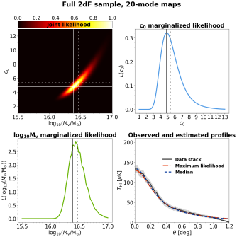
Figure 11: Results of the parameter estimation described in section 6.1, for the case of the full 2dF sample stacked on the 10-mode maps (left panel) and the 20-mode maps (right panel). In each case, we show the likelihood contours as a function of the two parameters $\log_{10}{(M_{\rm v}/\text{M}_{\odot})}$ and $c_{0,\rm HI}$ (top-left corner), the marginalized likelihood distribution as a function of $c_{0,\rm HI}$ alone (top-right corner) and $M_{\rm v}$ alone (bottom-left corner), and the comparison between the observed and estimated profiles (bottom-right). In the first three plots, the maximum likelihood estimates $\tilde{\Theta}$ are marked with solid lines, the median estimates $\hat{\Theta}$ with dashed lines. In the bottom-right corner, the observed profile (with associated uncertainty shown as a shaded region) is compared with the predictions computed using both sets of best-fit parameters.

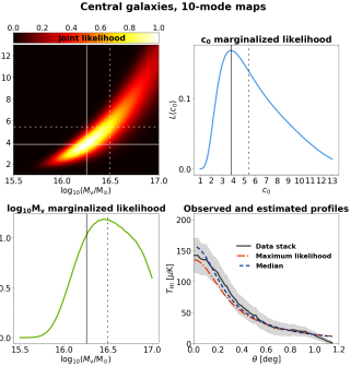
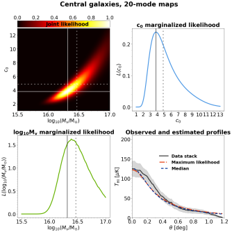
Figure 12: Same as in Fig. 11, but for the parameter estimation of the central galaxy sample.

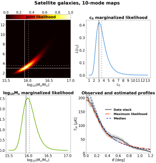
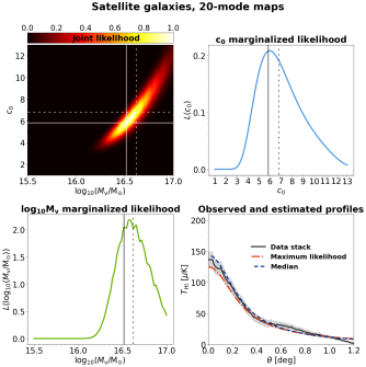
Figure 13: Same as in Figs. 11 and 12, but for the parameter estimation of the satellite galaxy sample.

6 Parameter estimation

The formalism described in Section 5 allows computing the expected observed brightness temperature profile for a generic halo. In this section, we consider the inverse problem of employing the observed profiles to estimate the corresponding halo properties.

6.1 Methodology and results

The methodology we employ has already been exploited in the literature to estimate the parameters governing the HIHM and the HI density profile; these parameters are typically fitted over DLA observables (Barnes & Haehnelt, 2014; Padmanabhan & Refregier, 2017) or numerical simulations (Villaescusa-Navarro et al., 2018). Here, for the first time, we apply this type of estimation directly against the reconstructed halo profiles. A shortcoming of our data-set, as already mentioned, is that it lacks a detailed characterisation of the mass distribution of the objects we are stacking. Given this uncertainty, we cannot fit for the parameters governing the HIHM relation. In contrast, since the size of the haloes we detect is unknown, we want to fix the HIHM relation and find the best-fit values for the halo mass to accommodate our results. As anticipated, although haloes with different sizes are merged in the stacking, this methodology would only provide us with a mean value for the mass representative of the full samples that we are stacking. For this aim we employ the HIHM functional form from Eq. (8) with the parameters (Eq. (5.1)) obtained by Padmanabhan & Kulkarni (2017) with a fit over low redshift observables. As per the halo density profile, we adopt the modified NFW profile from Eq. (10) and take the normalisation $c_{0,\rm HI}$ for the HI concentration parameter from Eq. (12) as our second free parameter. Another critical variable entering the computation of the observed halo profile (Eq. (20)) is the halo redshift. Since we are modelling the observed profile as produced by a single halo, we are also dealing with a single value of redshift. This time, we can fix it to the mean value from the redshifts of the stacked galaxies, i.e. $z=0.08$.

Our parameter space is then two-dimensional, and can be denoted as $\Theta=\{\log_{10}{(M_{\rm v}/\text{M}_{\odot})},c_{0,\rm HI}\}$ (given the high sensitivity of the profile amplitude on the virial mass, we found it more convenient to fit for its logarithm). For each point in this parameter space, Eq. (20) provides us with the corresponding profile $T_{\rm HI}^{\rm(theo)}(\theta;\Theta)$, which can be compared to any of the profiles plotted in Fig. 8. The goodness of the predicted profile to reproduce the observed ones can be assessed by a proper likelihood function; the point $\tilde{\Theta}$ that maximizes the likelihood value is taken as our best fit estimate for the combination of the two parameters. Notice that the correlation between bins that emerges from the covariance matrices plotted in Fig. 10 means that a simple chi-square estimation cannot be applied. We revert then to a more general multi-variate Gaussian likelihood function of the form:

$$\mathcal{L}(\Theta) = \dfrac{1}{\left[(2\pi)^{N}{\rm det}\,\mathcal{C}_{\rm T}\right]^{1/2}}\exp\left[-\dfrac{1}{2}\left(T_{\rm HI}^{\rm(theo)}(\Theta)-T_{\rm HI}\right)\right.$$ (22)

$$\times \left.\mathcal{C}_{\rm T}^{-1}\left(T_{\rm HI}^{\rm(theo)}(\Theta)-T_{\rm HI}\right)\right],$$

where $N$ is the number of bins in the angular separation from the halo centre, $T_{\rm HI}^{\rm(theo)}$ is the theoretical profile, $T_{\rm HI}$ is the reconstructed profile, and $\mathcal{C}_{\rm T}$ is the covariance matrix computed with Eq. (7). The factor multiplying the exponential is required to normalise the likelihood integral to unity.

The likelihood (Eq. (22)) computed for different combinations of the halo virial mass and the concentration parameter normalisation is plotted in the top-left corners of both panels in Figs. 11, 12 and 13 for the case of the full, central and satellite 2dF samples, respectively, each panel showing a different foreground removal case. The best fit parameter values $\tilde{\Theta}$ are overplotted with solid lines in all cases, and their intersection marks the point of maximum likelihood. These plots, however, are also essential in showing the resultant likelihood contours that can be used to extract the uncertainty associated with our estimates. For this aim, we marginalise the likelihood for each one of the two parameters and re-normalise to unit integral; the resultant function can then be regarded as the associated probability distribution. In the same figures, the top-right corner of each panel shows the marginalised likelihood as a function of $c_{0,\rm HI}$, and the bottom-left corner shows the marginalised likelihood as a function of $\log_{10}{(M_{\rm v}/\text{M}_{\odot})}$. Each of these marginalised functions is integrated to obtain the corresponding cumulative distribution function $F(\eta)$ (where $\eta=\log_{10}{(M_{\rm v}/\text{M}_{\odot})}$ or $\eta=c_{0,\rm HI}$). The percentiles of this distribution are used to estimate the uncertainty associated with our estimates: by defining the variables $\eta_{-}$, $\hat{\eta}$ and $\eta_{+}$ such as $F(\eta_{-})=0.16$, $F(\hat{\eta})=0.50$ and $F(\eta_{+})=0.84$, we compute the lower and upper uncertainties as $\sigma_{-}=\hat{\eta}-\eta_{-}$ and $\sigma_{+}=\eta_{+}-\hat{\eta}$. The quantity $\hat{\eta}$ is the median of the distribution and is a best-fit estimate alternative to the maximum-likelihood one.

In Table 3 we quote, for each chosen galaxy sample and foreground removal case, the maximum-likelihood estimates $\tilde{\Theta}=\{\log_{10}{(\tilde{M}_{\rm v}/\text{M}_{\odot})},\tilde{c}_{0,\rm HI}\}$ and the median estimates $\hat{\Theta}=\{\log_{10}{(\hat{M}_{\rm v}/\text{M}_{\odot})},\hat{c}_{0,\rm HI}\}$ with their uncertainties. Both the maximum likelihood $\tilde{\Theta}$ and median $\hat{\Theta}$ estimates are marked in the plots mentioned above with pairs of solid and dashed lines, respectively. Finally, the bottom-right panel of each figure shows the profile extracted from the stacks in comparison with the theoretical profiles computed using both sets of best-fit parameters $\tilde{\Theta}$ and $\hat{\Theta}$.

Table 3: Results of our parameter estimation analysis. For each 2dF sub-sample and foreground removal case, we quote the maximum likelihood estimates $\tilde{\Theta}$ and the median estimates $\hat{\Theta}$, as defined in Section 6.1.

		10-mode maps			20-mode maps
Full 2dF sample		$\log_{10}{(\tilde{M}_{\rm v}/\text{M}_{\odot})}=16.0$	$\log_{10}{(\hat{M}_{\rm v}/\text{M}_{\odot})}=16.1^{+0.1}_{-0.2}$		$\log_{10}{(\tilde{M}_{\rm v}/\text{M}_{\odot})}=16.4$	$\log_{10}{(\hat{M}_{\rm v}/\text{M}_{\odot})}=16.5^{+0.1}_{-0.2}$
		$\tilde{c}_{0,\rm HI}=3.0$	$\hat{c}_{0,\rm HI}=3.5^{+0.7}_{-1.0}$		$\tilde{c}_{0,\rm HI}=4.8$	$\hat{c}_{0,\rm HI}=5.3^{+1.1}_{-1.7}$
Central galaxies		$\log_{10}{(\tilde{M}_{\rm v}/\text{M}_{\odot})}=16.3$	$\log_{10}{(\hat{M}_{\rm v}/\text{M}_{\odot})}=16.5^{+0.3}_{-0.3}$		$\log_{10}{(\tilde{M}_{\rm v}/\text{M}_{\odot})}=16.3$	$\log_{10}{(\hat{M}_{\rm v}/\text{M}_{\odot})}=16.5^{+0.2}_{-0.3}$
		$\tilde{c}_{0,\rm HI}=3.8$	$\hat{c}_{0,\rm HI}=5.4^{+2.1}_{-3.5}$		$\tilde{c}_{0,\rm HI}=3.8$	$\hat{c}_{0,\rm HI}=4.9^{+1.5}_{-2.6}$
Satellite galaxies		$\log_{10}{(\tilde{M}_{\rm v}/\text{M}_{\odot})}=15.9$	$\log_{10}{(\hat{M}_{\rm v}/\text{M}_{\odot})}=16.0^{+0.1}_{-0.2}$		$\log_{10}{(\tilde{M}_{\rm v}/\text{M}_{\odot})}=16.5$	$\log_{10}{(\hat{M}_{\rm v}/\text{M}_{\odot})}=16.6^{+0.2}_{-0.2}$
		$\tilde{c}_{0,\rm HI}=3.0$	$\hat{c}_{0,\rm HI}=3.6^{+0.9}_{-1.4}$		$\tilde{c}_{0,\rm HI}=5.8$	$\hat{c}_{0,\rm HI}=6.8^{+1.7}_{-2.4}$

6.2 Discussion

The likelihood contour plots from Figs. 11 to 13 show the most likely combinations of the halo mass and concentration parameter that reproduce the reconstructed profiles. The size of the contours is representative of the uncertainty associated with the estimation of each parameter. We see that the contours obtained by stacking the full 2dF sample are narrower, a result of the higher statistics of the considered sample, while the contours for the central galaxy sample are the broadest. However, the main feature emerging from these plots is the tight correlation between the two parameters we fit for, that produces an evident elongation of the contours along the same direction in all cases. Qualitatively, such a correlation can be understood: the HIHM relation (Eq. (8)) implies that for virial masses above the turning point of $\sim 3\times 10^{11}\,\text{M}_{\odot}$ the HI halo mass grows slowly, approximately as $M_{\rm v}^{0.25}$. The virial radius, however, keeps growing as $M_{\rm v}^{1/3}$, and as a result, the density normalisation $\rho_{0}$ computed using Eq. (14) decreases for higher masses. In other words, with this model, higher virial masses determine shallower, more extended HI density profiles; a higher concentration parameter is then required to shrink the profile towards the centre and increase its peak amplitude.

The bottom-right panels of Figs. 11 to 13 show that the best-fit parameters associated with the maximum of the likelihood distribution are indeed effective in recovering the observed halo brightness temperature profile. The corresponding theoretical predictions, indeed, capture both the amplitude and shape of the reconstructed profiles. To assign uncertainties to the best-fit estimates, we computed the median of the contours following the procedure described above. The observed elongation of the likelihood profile is particularly visible in the marginalised likelihood plots, as it produces a clear positive skewness. As a result, the median estimates are always higher than the maximum-likelihood ones. However, it is interesting to notice how the median estimates are also very effective in reproducing the observed profiles, as the strong degeneracy between $M_{\rm v}$ and $c_{0,\rm HI}$ allows different combinations of the two parameters that yield very similar predictions. Both the maximum likelihood and the median estimates with their uncertainties are reported in table 3. The virial mass seems to be better constrained, with a relative error typically below 2%, but the uncertainty on the concentration parameter can get higher than 50%.

We can now make some considerations on the significance of our findings. Our results suggest very low values for the normalisation of the concentration parameter (typically $\lesssim 7$). In the literature, although the concentration parameter for neutral gas is generally found to be higher than for the case of dark matter, its actual value is still largely unconstrained. For example, we can quote the estimate $c_{0,\rm HI}\simeq 25$ from Barnes & Haehnelt (2010) and Barnes & Haehnelt (2014), or $c_{0,\rm HI}\simeq 133$ from (Padmanabhan & Kulkarni, 2017). However, Villaescusa-Navarro et al. (2014) found that much lower values for the concentration, $c_{0,\rm HI}\sim 3$, are favoured by numerical simulations, a result compatible with our findings. All the estimates mentioned above are fitted over high redshift observables, typically in the range of $z\sim 2$ to 4; we provide here for the first time an estimate for very low redshift, $z\sim 0.08$. We also need to remind that a direct comparison with galactic-halo estimates may be misleading, as this concentration is not referred to diffuse gas in the haloes, but rather to the integrated contribution of the HI emission from different galaxies.

The other parameter we fitted for, the virial halo mass, yields very high values averaging at $M_{\rm v}\sim 2\times 10^{16}\,\text{M}_{\odot}$, which is the scale of the most massive haloes in the Universe. This estimate can actually be a biased result because of the assumptions made in our theoretical modelling, as it is now confirmed that our chosen functional form for the HIHM (Eq. (8)) is being applied beyond the mass range over which the parameters in Eq. (5.1) were fitted ($\sim 10^{11}$ to $10^{14}\,\text{M}_{\odot}$, Padmanabhan & Kulkarni, 2017). Nonetheless, it can be double-checked quickly: the virial radius for a halo of mass $M_{\rm v}=10^{16}\,\text{M}_{\odot}$ is approximately 5.3 Mpc. If that halo is located at $z=0.08$, the angular radius it subtends is approximately 1 deg. This scale is indeed the typical extension of the profiles we detect in the stack maps. Plus, by taking $c_{0,\rm HI}=4$, the resultant angular size corresponding to the scale radius $r_{\rm s}$ is $\sim 0.25\,\text{deg}$, and we do observe a flexion in the profiles around $\theta\sim 0.3\,\text{deg}$. This rough estimate serves to verify that our stacks do indeed reveal the emission towards very massive objects. The observed HI signal likely proceeds from the HI locked inside the gas richest galaxies in the 2dF sample, to which we should add the contribution from all the optically faint, HI-rich galaxies that were not detected in the 2dF survey. As the low resolution of the intensity mapping technique probes the HI large-scale fluctuations, the estimated masses weigh the locally HI-brighter regions made by the contribution of all those galaxies, possibly assembled in large groups or clusters.

It is then interesting to compare this finding with the results presented in Papastergis et al. (2013), according to which HI-rich galaxies are the least clustered population type, so that cluster member galaxies are expected not to be included in HI-selected samples. Neverthless, other studies pointed towards satellite galaxies located in the outskirts of galaxy groups and clusters to host a significant amount of HI (Lah et al., 2009; Baugh et al., 2019; Guo et al., 2020). Now, the results of our blind stacks do not allow to draw further conclusions about the actual origin of the detected HI signal, although a hint may come from the comparison between the different 2dF subsamples we used. We have already pointed out in section 4 how the full sample shows features in between the other two, reinforcing the hypothesis that the latter are tracing galaxies belonging to different environments. We note that, for the central galaxy sample, we are most likely centring our stacks over groups and clusters of galaxies: we find, as a result, a dilution of the resultant HI profile, which appears less bright in the centre, and more slowly decaying towards larger radii. The stack of satellite galaxies, instead, yields brighter and more concentrated profiles. This phenomenon can be in agreement with the finding that even cluster-member galaxies, when located in the cluster outskirts, can be HI-rich. However, these conclusions are more evident when comparing the reconstructed profiles than the estimated parameters, because the tight degeneracy between $M_{\rm v}$ and $c_{0,\rm HI}$ easily overrides the marginal difference provided by the selected samples. Still, looking again at table 3, we can point out some differences. For the 20-mode removal case, the mass estimate is consistent within a 1% variation across different samples, while the concentration parameter is the highest for the satellite sample, the lowest for the central sample, and intermediate for the full sample. This result is in agreement with our hypothesis that the satellite galaxies trace better the HI distribution, yielding more concentrated profiles. The same is not valid, however, for the 10-mode removal case, where we obtain remarkably similar results for the full and satellite samples, while the central galaxy stack provides higher estimates for both the estimated mass and concentration parameter. Notice anyway that the 10-mode central galaxy stack was from the beginning the most irregular (Fig. 5), the resultant likelihood contours are the broadest, and the corresponding uncertainties are the largest; this case is then probably not as clean as the other ones. We can finally observe that the 10-mode case generally favours lower masses and concentration parameters than the 20-mode case. This situation may be a result of the 20-mode maps having lost HI signal in the foreground removal process, which results in more irregular stacks that are artificially broadened in the symmetrisation process. Broader profiles, in turn, require higher mass values, and, because of the degeneracy, higher concentrations.

To summarise, we can state that although our selection of specific 2dF sub-samples provides hints of different results, in terms of the corresponding stacks and extracted profiles, the resultant estimates are generally compatible with each other. Therefore, we can quote as our final results the estimates obtained with the full 2dF sample, which benefits from its more significant statistics. The strong degeneracy between $M_{\rm v}$ and $c_{0,\rm HI}$ is an additional factor that hinders possible differences in the final estimates arising from the use of a specific sub-sample. A higher variation is instead produced by choice of the 10 or 20-mode maps, although we cannot assess whether the differences arise from an excess of foreground residuals in the former or removal of physical HI emission in the latter. This consideration shows that proper foreground removal remains a critical element in the exploitation of 21-cm intensity maps for constraining the HI abundance in haloes.

7 Conclusions

This paper tackles the search for neutral hydrogen in the cosmic web using 21-cm maps. The goal is to measure the HI brightness temperature profile proceeding from the merged contribution of galaxies in massive large-scale haloes. The signal is searched for by blindly stacking map regions centred on the fiducial positions extracted from a galaxy catalogue. This approach requires to use a data set with high available statistics, and the substantial overlap between the spatial distribution of catalogue(s) and maps. Our choice reverted therefore to a set of 21-cm maps obtained with the Parkes telescope over the volume spanned by the 2dF galaxy catalogue, covering a large sky area of $\sim 1,300\,\text{deg}^{2}$ over the redshift range $0.06\lesssim z\lesssim 0.08$. The same data set proved effective in Tramonte et al. (2019) for a similar search of neutral gas in cosmic web filaments.

We considered three different galactic samples extracted from the 2dF catalogue. These are the full sample comprising all the galaxies sharing the map volume, a sample made only of the locally brightest galaxies, which more likely trace the centre of galaxy clusters and groups, and the associated complementary sample of satellite galaxies. This subdivision allows us to compare the profiles obtained with galaxies belonging to different local environments. Altogether, we employed 48,430 galaxies for the full sample, 13,979 galaxies for the central sample and 34,361 galaxies for the satellite sample. We also considered two versions of the Parkes maps, obtained by removing a different number of modes (10 and 20) in a PCA foreground cleaning algorithm, to assess to what extent possible foreground residuals affect our results.

For all six combinations of 2dF samples and foreground removal cases we provided the resultant stack maps, which clearly show the detection of the halo HI emission at a level of $\sim 200\,\mu\text{K}$ for the 10-mode removal case and of $\sim 150\,\mu\text{K}$ for 20-mode removal case. This difference can be due to either the presence of radio foreground residuals in the 10-mode maps or the excessive removal of HI signal in the 20-mode maps. In both cases, the satellite galaxy sample yields more rounded and shrunk peaks, while the central galaxy sample produces more irregular and extended peaks, with the full 2dF sample showing intermediate features. The corresponding radial profiles were obtained by circularly symmetrising the stacks and considering the mean value of pixels found within specified angular separation bins from the halo centre. For each 2dF sample and foreground removal choice, we repeated the same analysis using a set of 500 replicas of the galaxy catalogue obtained by randomising the object equatorial coordinates. The dispersion of the corresponding profiles across different realisations provides an estimate of the uncertainty associated with our measurements, and of the correlation between pairs of radial bins. The detection significance at the profile peak is always above $5\sigma$ and even higher than $12\sigma$ for the full 2dF sample. The comparison of profiles obtained with different foreground removed maps or 2dF samples confirms the considerations already drawn by comparing the associated stack maps. More importantly, we quantified the extension of the profiles out to 1 deg from the halo centre. This is considerably higher than the 14’ FWHM Parkes beam, which ensures these halo profiles are spatially resolved.

The second half of this work was dedicated to the theoretical modelling of the observed HI emission. We first outlined how to compute the mean observed HI brightness temperature profile expected for a generic halo of given mass and redshift. We adopted a functional form for the HI-halo mass (HIHM) relation directly fitted over low-redshift observations of HI-rich galaxies, and a general modified NFW shape to model the HI radial distribution. We compared then the theoretically computed brightness temperature profile with the ones extracted from our stacks; the latter were considered as as produced by a single type of haloes, whose properties (mass, redshift and HI concentration parameter) are a mean of the corresponding sample members. We fixed the redshift to the mean of the samples ($z=0.08$) and fitted for the logarithm of the virial halo mass, $\log_{10}{(M_{\rm v}/\text{M}_{\odot})}$, and for the normalisation of the HI concentration parameter, $c_{0,\rm HI}$. We built a two-dimensional likelihood distribution computed with a general multi-variate Gaussian form that takes into account the observed correlation between angular bins. The resultant contours showed a clear degeneracy between the halo mass and the concentration parameters, which makes it difficult to extract a best-fit value without the assumption of any priors on the halo mass. We found that, although marginal variations arise from the use of different 2dF samples, the estimates are mostly compatible, and favour the values $M_{\rm v}\simeq 1.3\times 10^{16}\,\text{M}_{\odot}$, $c_{0,\rm HI}\simeq 3.5$ for the 10-mode removal case and $M_{\rm v}\simeq 3.2\times 10^{16}\,\text{M}_{\odot}$, $c_{0,\rm HI}\simeq 5.3$ for the 20-mode removal case.

The recovered halo mass is very high and corresponds to the largest haloes found in the cosmic web. This finding is consistent with the observed angular extension of the profiles, and it is most likely produced by the combined contribution of neutral gas contained in different galaxies found in groups and clusters. The Parkes 21-cm maps we employed, indeed, record the large-scale fluctuations of HI and do not allow to resolve individual galactic objects. The recovered concentration is lower than the values typically favoured by studies of HI in haloes, probably a result of the HI gas being locked inside galaxies and not being diffuse inside the massive haloes we probe. However, it is still a largely unconstrained parameter, and our estimates provide a direct measurement at low redshift.

The most crucial element entering our theoretical prediction is perhaps the HIHM relation, which is applied to masses outside the range over which it was tested. This procedure is a source of possible bias for our final estimation. But given the intrinsic uncertainty on the mass of the objects we are stacking, we cannot fit at the same time for the HIHM parameters. It would be useful, in this sense, to deal with a halo sample with a characterised mass distribution. Such data set would allow to fully model the cross-correlation between the 21-cm and galaxy sample, which in real space translates into the mean radial profile around halo centres. The comparison of such a model with the observed profiles would allow fitting for the parameters governing the HIHM.

In conclusion, we stress that the most important results obtained in this study are the feasibility of measuring the HI content in large-scale haloes using 21-cm maps, and the possibility of testing theoretical models on the reconstructed profiles. Most of the theoretical modelling was previously tested on galactic-scale haloes, which are not accessible with the resolution of our maps. Still, we applied it to the large scale haloes we detected, formally treating their effective profile as if it was produced by a diffuse gas component. The resulting high masses and low concentrations remind us that we are in fact probing super-galactic scales. Nonetheless, this paper presents a novel methodology that can be applied to future, more suitable data sets: the next generation of radio interferometric experiment as MeerKAT (Jonas & MeerKAT Team, 2016), ASKAP (Meyer, 2009) and the future Square Kilometer Array (Braun et al., 2015) is expected to provide large-scale 21-cm maps with higher resolution, which may enable to extend this study to the proper galactic-scale haloes. It would also be interesting to apply our stack on the combination of the ALFALFA survey legacy catalogue with the corresponding HI cubes (the latter are not publicly available at present), or to the combination of the BOSS-LOWZ galaxy catalogue (Dawson et al., 2013) with maps resulting from the ongoing Commensal Radio Astronomy FAST Survey (CRAFTS, Zhang et al., 2019). The latter is scheduled to map the HI distribution over $\sim 20,000\,\text{deg}^{2}$ and up to $z\sim 0.35$, with a $\sim 3.24^{\prime}$ resolution that allows to resolve smaller galaxy group scales with typical halo masses of $10^{13}\,\text{M}_{\odot}$.

References

- Anderson et al. (2018) Anderson C. J., et al., 2018, MNRAS, 476, 3382
- Bagla et al. (2010) Bagla J. S., Khandai N., Datta K. K., 2010, MNRAS, 407, 567
- Barnes & Haehnelt (2010) Barnes L. A., Haehnelt M. G., 2010, MNRAS, 403, 870
- Barnes & Haehnelt (2014) Barnes L. A., Haehnelt M. G., 2014, MNRAS, 440, 2313
- Baugh et al. (2019) Baugh C. M., et al., 2019, MNRAS, 483, 4922
- Bigiel & Blitz (2012) Bigiel F., Blitz L., 2012, ApJ, 756, 183
- Braun et al. (2015) Braun R., Bourke T., Green J. A., Keane E., Wagg J., 2015, Advancing Astrophysics with the Square Kilometre Array (AASKA14), p. 174
- Bregman et al. (2019) Bregman J., et al., 2019, BAAS, 51, 450
- Bryan & Norman (1998) Bryan G. L., Norman M. L., 1998, ApJ, 495, 80
- Bullock et al. (2001) Bullock J. S., Kolatt T. S., Sigad Y., Somerville R. S., Kravtsov A. V., Klypin A. A., Primack J. R., Dekel A., 2001, MNRAS, 321, 559
- Calette et al. (2018) Calette A. R., Avila-Reese V., Rodríguez-Puebla A., Hernández-Toledo H., Papastergis E., 2018, Rev. Mex. Astron. Astrofis., 54, 443
- Cen & Ostriker (1999) Cen R., Ostriker J. P., 1999, ApJ, 514, 1
- Cen & Ostriker (2006) Cen R., Ostriker J. P., 2006, ApJ, 650, 560
- Chang et al. (2010) Chang T.-C., Pen U.-L., Bandura K., Peterson J. B., 2010, Nature, 466, 463
- Cole et al. (2000) Cole S., Lacey C. G., Baugh C. M., Frenk C. S., 2000, MNRAS, 319, 168
- Colless et al. (2001) Colless M., et al., 2001, MNRAS, 328, 1039
- Condon & Ransom (2016) Condon J. J., Ransom S. M., 2016, Essential Radio Astronomy
- Cui et al. (2019) Cui W., et al., 2019, MNRAS, 485, 2367
- Cunnama et al. (2014) Cunnama D., Andrianomena S., Cress C. M., Faltenbacher A., Gibson B. K., Theuns T., 2014, MNRAS, 438, 2530
- Davé et al. (1999) Davé R., Hernquist L., Katz N., Weinberg D. H., 1999, ApJ, 511, 521
- Davis et al. (2001) Davis M., Newman J. A., Faber S. M., Phillips A. C., 2001, in Cristiani S., Renzini A., Williams R. E., eds, Deep Fields. p. 241 (arXiv:astro-ph/0012189), doi:10.1007/10854354_66
- Dawson et al. (2013) Dawson K. S., et al., 2013, AJ, 145, 10
- Dawson et al. (2016) Dawson K. S., et al., 2016, AJ, 151, 44
- Delhaize et al. (2013) Delhaize J., Meyer M. J., Staveley-Smith L., Boyle B. J., 2013, MNRAS, 433, 1398
- Di Matteo et al. (2005) Di Matteo T., Springel V., Hernquist L., 2005, Nature, 433, 604
- Drinkwater et al. (2010) Drinkwater M. J., et al., 2010, MNRAS, 401, 1429
- Duffy et al. (2012) Duffy A. R., Kay S. T., Battye R. A., Booth C. M., Dalla Vecchia C., Schaye J., 2012, MNRAS, 420, 2799
- Eckert et al. (2015) Eckert D., et al., 2015, Nature, 528, 105
- Font-Ribera et al. (2012) Font-Ribera A., et al., 2012, J. Cosmology Astropart. Phys., 2012, 059
- Fu et al. (2010) Fu J., Guo Q., Kauffmann G., Krumholz M. R., 2010, MNRAS, 409, 515
- Genel et al. (2010) Genel S., Bouché N., Naab T., Sternberg A., Genzel R., 2010, ApJ, 719, 229
- Génova-Santos et al. (2015) Génova-Santos R., Atrio-Barandela F., Kitaura F.-S., Mücket J. P., 2015, ApJ, 806, 113
- Gong et al. (2019) Gong Y., Ma Y.-Z., Tanimura H., 2019, MNRAS, 486, 4904
- Guo et al. (2017) Guo H., Li C., Zheng Z., Mo H. J., Jing Y. P., Zu Y., Lim S. H., Xu H., 2017, ApJ, 846, 61
- Guo et al. (2020) Guo H., Jones M. G., Haynes M. P., Fu J., 2020, ApJ, 894, 92
- Haider et al. (2016) Haider M., Steinhauser D., Vogelsberger M., Genel S., Springel V., Torrey P., Hernquist L., 2016, MNRAS, 457, 3024
- Haynes et al. (2018) Haynes M. P., et al., 2018, ApJ, 861, 49
- Hernández-Monteagudo et al. (2015) Hernández-Monteagudo C., Ma Y.-Z., Kitaura F. S., Wang W., Génova-Santos R., Macías-Pérez J., Herranz D., 2015, Physical Review Letters, 115, 191301
- Hoppmann et al. (2015) Hoppmann L., Staveley-Smith L., Freudling W., Zwaan M. A., Minchin R. F., Calabretta M. R., 2015, MNRAS, 452, 3726
- Horii et al. (2017) Horii T., Asaba S., Hasegawa K., Tashiro H., 2017, PASJ, 69, 73
- Jonas & MeerKAT Team (2016) Jonas J., MeerKAT Team 2016, in MeerKAT Science: On the Pathway to the SKA. p. 1
- Jones et al. (2009) Jones D. H., et al., 2009, MNRAS, 399, 683
- Kim et al. (2011) Kim H.-S., Baugh C. M., Benson A. J., Cole S., Frenk C. S., Lacey C. G., Power C., Schneider M., 2011, MNRAS, 414, 2367
- Kim et al. (2017) Kim H.-S., Wyithe J. S. B., Baugh C. M., Lagos C. d. P., Power C., Park J., 2017, MNRAS, 465, 111
- Lah et al. (2009) Lah P., et al., 2009, MNRAS, 399, 1447
- Liu & Tegmark (2012) Liu A., Tegmark M., 2012, MNRAS, 419, 3491
- Longair (1998) Longair M. S., 1998, Galaxy formation
- Ma et al. (2015) Ma Y.-Z., Van Waerbeke L., Hinshaw G., Hojjati A., Scott D., Zuntz J., 2015, J. Cosmology Astropart. Phys., 9, 046
- Macciò et al. (2007) Macciò A. V., Dutton A. A., van den Bosch F. C., Moore B., Potter D., Stadel J., 2007, MNRAS, 378, 55
- Maller & Bullock (2004) Maller A. H., Bullock J. S., 2004, MNRAS, 355, 694
- Martin et al. (2010) Martin A. M., Papastergis E., Giovanelli R., Haynes M. P., Springob C. M., Stierwalt S., 2010, ApJ, 723, 1359
- Martizzi et al. (2019) Martizzi D., et al., 2019, MNRAS, 486, 3766
- Masui et al. (2013) Masui K. W., et al., 2013, ApJ, 763, L20
- Meyer (2009) Meyer M., 2009, in Panoramic Radio Astronomy: Wide-field 1-2 GHz Research on Galaxy Evolution. p. 15 (arXiv:0912.2167)
- Meyer et al. (2004) Meyer M. J., et al., 2004, MNRAS, 350, 1195
- Moster et al. (2010) Moster B. P., Somerville R. S., Maulbetsch C., van den Bosch F. C., Macciò A. V., Naab T., Oser L., 2010, ApJ, 710, 903
- Moster et al. (2013) Moster B. P., Naab T., White S. D. M., 2013, MNRAS, 428, 3121
- Navarro et al. (1996) Navarro J. F., Frenk C. S., White S. D. M., 1996, ApJ, 462, 563
- Obreschkow et al. (2009) Obreschkow D., Klöckner H. R., Heywood I., Levrier F., Rawlings S., 2009, ApJ, 703, 1890
- Padmanabhan (2002) Padmanabhan T., 2002, Theoretical Astrophysics - Volume 3, Galaxies and Cosmology, doi:10.2277/0521562422.
- Padmanabhan & Kulkarni (2017) Padmanabhan H., Kulkarni G., 2017, MNRAS, 470, 340
- Padmanabhan & Refregier (2017) Padmanabhan H., Refregier A., 2017, MNRAS, 464, 4008
- Padmanabhan et al. (2017) Padmanabhan H., Refregier A., Amara A., 2017, MNRAS, 469, 2323
- Papastergis et al. (2013) Papastergis E., Giovanelli R., Haynes M. P., Rodríguez-Puebla A., Jones M. G., 2013, ApJ, 776, 43
- Peebles (1980) Peebles P. J. E., 1980, The large-scale structure of the universe
- Pen et al. (2009) Pen U.-L., Staveley-Smith L., Peterson J. B., Chang T.-C., 2009, MNRAS, 394, L6
- Planck Collaboration et al. (2013) Planck Collaboration et al., 2013, A&A, 557, A52
- Pontzen et al. (2008) Pontzen A., et al., 2008, MNRAS, 390, 1349
- Popping et al. (2009) Popping A., Davé R., Braun R., Oppenheimer B. D., 2009, A&A, 504, 15
- Pritchard & Loeb (2008) Pritchard J. R., Loeb A., 2008, Phys. Rev. D, 78, 103511
- Prochaska & Wolfe (2009) Prochaska J. X., Wolfe A. M., 2009, ApJ, 696, 1543
- Rhee et al. (2013) Rhee J., Zwaan M. A., Briggs F. H., Chengalur J. N., Lah P., Oosterloo T., van der Hulst T., 2013, MNRAS, 435, 2693
- Rhee et al. (2018) Rhee J., Lah P., Briggs F. H., Chengalur J. N., Colless M., Willner S. P., Ashby M. L. N., Le Fèvre O., 2018, MNRAS, 473, 1879
- Schlegel et al. (2009) Schlegel D., White M., Eisenstein D., 2009, in astro2010: The Astronomy and Astrophysics Decadal Survey. p. 314 (arXiv:0902.4680)
- Sheth & Tormen (2002) Sheth R. K., Tormen G., 2002, MNRAS, 329, 61
- Staveley-Smith et al. (1996) Staveley-Smith L., et al., 1996, Publ. Astron. Soc. Australia, 13, 243
- Switzer et al. (2015) Switzer E. R., Chang T.-C., Masui K. W., Pen U.-L., Voytek T. C., 2015, ApJ, 815, 51
- Takeuchi et al. (2014) Takeuchi Y., Zaroubi S., Sugiyama N., 2014, MNRAS, 444, 2236
- Tanimura et al. (2019) Tanimura H., et al., 2019, MNRAS, 483, 223
- Tanimura et al. (2020) Tanimura H., et al., 2020, MNRAS, 491, 2318
- Tramonte et al. (2019) Tramonte D., Ma Y.-Z., Li Y.-C., Staveley-Smith L., 2019, MNRAS, 489, 385
- Van Waerbeke et al. (2014) Van Waerbeke L., Hinshaw G., Murray N., 2014, Phys. Rev. D, 89, 023508
- Vazza et al. (2019) Vazza F., Ettori S., Roncarelli M., Angelinelli M., Brüggen M., Gheller C., 2019, A&A, 627, A5
- Villaescusa-Navarro et al. (2014) Villaescusa-Navarro F., Viel M., Datta K. K., Choudhury T. R., 2014, J. Cosmology Astropart. Phys., 2014, 050
- Villaescusa-Navarro et al. (2018) Villaescusa-Navarro F., et al., 2018, ApJ, 866, 135
- Walker et al. (2019) Walker S., et al., 2019, BAAS, 51, 218
- Wang et al. (2014) Wang J., et al., 2014, MNRAS, 441, 2159
- Wolfe et al. (2005) Wolfe A. M., Gawiser E., Prochaska J. X., 2005, ARA&A, 43, 861
- Zappacosta et al. (2002) Zappacosta L., Mannucci F., Maiolino R., Gilli R., Ferrara A., Finoguenov A., Nagar N. M., Axon D. J., 2002, A&A, 394, 7
- Zhang et al. (2019) Zhang K., et al., 2019, Science China Physics, Mechanics, and Astronomy, 62, 959506
- Zoldan et al. (2017) Zoldan A., De Lucia G., Xie L., Fontanot F., Hirschmann M., 2017, MNRAS, 465, 2236
- Zwaan et al. (2005) Zwaan M. A., Meyer M. J., Staveley-Smith L., Webster R. L., 2005, MNRAS, 359, L30
- de Graaff et al. (2019) de Graaff A., Cai Y.-C., Heymans C., Peacock J. A., 2019, A&A, 624, A48