Scalable multiphoton generation from cavity-synchronized single-photon sources

Abstract

We propose an efficient, scalable and deterministic scheme to generate up to hundreds of indistinguishable photons over multiple channels, on demand. Our design relies on multiple single-photon sources, each coupled to a waveguide, and all of them interacting with a common cavity mode. The cavity synchronizes and triggers the simultaneous emission of one photon by each source, which are collected by the waveguides. For a state-of-the-art circuit QED implementation, this scheme supports the creation of single photons with purity, indistinguishability, and efficiency of $99\%$ at rates of $\sim$MHz. We also discuss conditions to create a device to produce 30-photon simultaneously with efficiency above $70\%$ at a rate of hundreds of kHz. This is several orders of magnitude more efficient than previous demultiplexed sources for boson sampling, and enables the realization of deterministic multi-photon sources and scalable quantum information processing with photons.

I Introduction and main results

Efficient sources of single and indistinguishable photons Eisaman et al. (2011); Senellart et al. (2017); Slussarenko and Pryde (2019) are a fundamental requirement to perform all kinds of quantum information tasks with photons: photonic quantum computation Knill et al. (2001); Kok et al. (2007); Tiecke et al. (2014); Tiarks et al. (2016); Takeda and Furusawa (2019), networking Lodahl (2017), simulation Aspuru-Guzik and Walther (2012); Hartmann (2016), communication Briegel et al. (1998); Sangouard et al. (2011); Llewellyn et al. (2019), cryptography Gisin et al. (2002), metrology Motes et al. (2015); Ge et al. (2018), boson sampling Brod et al. (2019); Wang et al. (2017); Loredo et al. (2017); Wang et al. (2019a), or even quantum optical neural networks Steinbrecher et al. (2019). Scaling up these protocols requires the generation of a large product-state of $N\gg 1$ indistinguishable photons,

$$\ket{\Psi_{N}}=\ket{1}_{1}\otimes\ket{1}_{2}\otimes\dots\otimes\ket{1}_{N},$$ (1)

propagating along $N$ or more channels. The generation of this state with high fidelity and efficiency demands the use of nearly deterministic, nearly identical and perfectly synchronized single-photon sources (SPSs), each of them producing just one photon.

The best on-demand SPSs for this task rely on few-level quantum systems Fischer et al. (2016), which can be deterministically excited He and Barkai (2006); He (2006) and decay spontaneously, producing individual photons that are collected into the desired channels. The great experimental progress in controlling single quantum systems with cavity-enhanced light-matter interactions has allowed many realizations of nearly deterministic SPSs. A long list of setups includes single atoms McKeever et al. (2004); Hijlkema et al. (2007), single molecules Brunel et al. (1999); Ahtee et al. (2009); Rezai et al. (2018), trapped ions Almendros et al. (2009); Stute et al. (2012); Higginbottom et al. (2016); Sosnova et al. (2018), and atomic ensembles Chou et al. (2004); Matsukevich et al. (2006); Farrera et al. (2016); Ripka et al. (2018), as well as solid-state systems Aharonovich et al. (2016) such as quantum dots Santori et al. (2002); Nawrath et al. (2019); Wang et al. (2019b); Schnauber et al. (2019); Thoma et al. (2016); Dusanowski et al. (2019); Kiršanskė et al. (2017); Liu et al. (2018); Uppu et al. (2020) or color centers in diamond Rodiek et al. (2017); Sipahigil et al. (2014); Alléaume et al. (2004); Gaebel et al. (2004); Wu et al. (2007); Babinec et al. (2010); Tchernij et al. (2017); Neu et al. (2011); Schröder et al. (2011); Wang et al. (2019c). In the microwave regime, superconducting quantum circuits have been used to create nearly deterministic SPSs Houck et al. (2007); Pechal et al. (2014); Peng et al. (2016); Forn-Díaz et al. (2017); Gasparinetti et al. (2017); Pfaff et al. (2017); Eder et al. (2018); Zhou et al. (2020), which have the advantage of being externally tuneable Peng et al. (2016); Forn-Díaz et al. (2017); Pfaff et al. (2017), fast Pechal et al. (2014); Zhou et al. (2020), and readily integrated on-chip with very low losses Zhou et al. (2020). Currently, quantum dots in micro-pillar cavities are proving the best overall numbers including generation efficiencies, distinguishability, and single-photon purity Reimer and Cher (2019); Wang et al. (2019c); Uppu et al. (2020), but it is hard to manufacture many of them identically, and tuning them also remains elusive for more than two emitters Patel et al. (2010); Flagg et al. (2010); Moczała-Dusanowska et al. (2019); Ellis et al. (2018); Kambs and Becher (2018).

Despite remarkable experimental progress, scaling up to large number of identical SPSs remains a great challenge Slussarenko and Pryde (2019); Wang et al. (2019a); Kaneda and Kwiat (2019); Hummel et al. (2019); Lenzini et al. (2017). Active optical multiplexing is a promising alternative which is based on repeating the single-photon generation—in time Pittman et al. (2002); Kaneda et al. (2015); Kaneda and Kwiat (2019); Xiong et al. (2016); Mendoza et al. (2016), space Migdall et al. (2002); Ma et al. (2011); Shapiro and Wong (2007); Collins et al. (2013); Francis-Jones et al. (2016); Spring et al. (2017), or frequency Grimau Puigibert et al. (2017); Joshi et al. (2018); Hiemstra et al. (2019)—and then on synchronizing and rerouting the emitted photons using adaptive delay lines and switches. This method, originally developed to increase the efficiency of heralded SPSs Pittman et al. (2002); Migdall et al. (2002); Kaneda and Kwiat (2019); Christ and Silberhorn (2012), has been adapted to prepare $N$-photon states (1) using just one nearly deterministic source Lenzini et al. (2017); Wang et al. (2017); Loredo et al. (2017); Wang et al. (2019a); Antón et al. (2019); Hummel et al. (2019). This temporal-to-spatial demultiplexing requires a high quality SPS that can emit a long stream nearly indistinguishable photons Ding et al. (2016); Somaschi et al. (2016); Liu et al. (2018); Dusanowski et al. (2019); Uppu et al. (2020), as well as an accurate circuit that demultiplexes, routes and synchronizes the photons into multiple spatial channels. This technique enabled boson sampling with multi-photon states (1) from $N=3$ to $N=14$ photons, albeit at a low photon rate of $\sim$kHz to $\sim$mHz Lenzini et al. (2017); Wang et al. (2017); Loredo et al. (2017); Wang et al. (2019a); Antón et al. (2019); Hummel et al. (2019).

Apart from errors in the collection and detection of photons, optical multiplexing schemes are inherently slow and suffer from increased losses due to delay lines Francis-Jones et al. (2016); Nunn et al. (2013) and optical switches of the synchronizing circuit Bonneau et al. (2015); Lenzini et al. (2017); Gimeno-Segovia et al. (2017). The probability $P_{N}$ of generating the state $\ket{\psi_{N}}$—also called $N$-photon efficiency—is the product Lenzini et al. (2017)

$$P_{N}=({\cal P}_{1})^{N}S_{N},$$ (2)

of the probability ${\cal P}_{1}$ of generating an individual photon on each of the $N$ channels independently, times the correlation error $S_{N}$ introduced by the circuit. An ideal scheme should scale exponentially $(S_{N}=1)$, creating $N$ synchronous and completely uncorrelated photons. However, typical active demultiplexing schemes introduce errors that scale as $S_{N}=\frac{1}{N}\left[\eta^{N}+(N-1)\left(\frac{1-\eta}{N-1}\right)^{N}\right]$ Lenzini et al. (2017), where $\eta$ characterizes the switching efficiency. Imperfect switching is a critical issue in any large photonic circuit Li et al. (2015), but even in the limit of lossless switches ($\eta=1$), the demultiplexing scheme introduces a detrimental factor $S_{N}=1/N$ to the scaling in Eq. (2). This can significantly limit the achievable $N$-photon efficiencies in practical applications such as boson sampling.

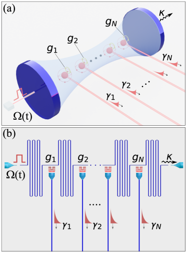
Figure 1: Cavity-QED scheme for deterministically generating a large number of synchronized and independent single-photons. (a) Idealized implementation with $N$ two-level emitters coupled to a common driven cavity mode. Each emitter additionally couples to independent output channels, which collect the $N$ emitted single-photons on parallel for later usage. (b) Efficient on-chip implementation using circuit-QED. Here, transmon qubits realize the $N$ two-level emitters, each of them capacitively coupled to an independent transmission-line antenna and to a common transmission-line resonator. Controlling the shape $\Omega(t)$ of the resonator drive, we can trigger all SPSs simultaneously and on-demand. The $N$ emitted microwave single-photons are collected by the on-chip antennas with high efficiency. These antennas are also used to send a DC current to each qubit and calibrate their frequencies into resonance with the resonator drive.

In this work, we propose a scheme to synchronize deterministic SPSs and generate $N$ photons with a negligible correlation error $S_{N}\approx 1$. The emitters reside in a bad cavity, and interact both with the common electromagnetic mode and with independent waveguides [cf. Fig. 1]. A strong coherent drive acting on the cavity excites the emitters in a perfectly synchronized way. When the drive ends, all emitters relax, producing individual photons that are collected by the waveguides. If the emitters relax faster than the timescale of cavity-mediated correlations, the photons are nearly independent and approach the state $\ket{\psi_{N}}.$ In a thorough study, we identify the optimal parameter conditions to suppress residual cavity-mediated interactions and super-radiance. Using master equation and quantum trajectories (QT) simulations, we characterize the performance and scaling of the synchronized multiphoton generation, accounting for imperfections and realistic noise sources. In particular, we find that the $N$-photon efficiency $P_{N}$ scales exponentially as in Eq. (2), except for an almost negligible quadratic deviation in $N$,

$$S_{N}=1+\epsilon N(N-1).$$ (3)

The correction factor $\epsilon$ stems from residual cavity-induced correlations. For realistic experimental conditions at the optimal working point, we find that $\epsilon\sim 10^{-8}-10^{-6}$, making the multiphoton generation scheme scalable up to $N\sim 100-1000\ll\epsilon^{-1/2}$, depending on the implementation and the noise sources.

To show the favorable scaling of the scheme in a realistic setup, we study a circuit-QED implementation with flux-tunable transmon emitters and microwave transmission lines DiCarlo et al. (2009); Barends et al. (2013); Pechal et al. (2014), considering dephasing noise, internal loss, and disorder. As shown in Fig. 1(b), this implementation is fully integrated on-chip, which allows the output antennas to have collection and transmission efficiencies above $99\%$ Zhou et al. (2020). For a strongly driven cavity, we show it is feasible to build microwave SPSs with single-photon purity and indistinguishability above $99\%$, as measured via standard Hanbury Brown and Twiss (HBT), and Hong-Ou-Mandel (HOM) experiments. Most importantly, we predict an overall single-photon efficiency or brightness of ${\cal P}_{1}\gtrsim 0.99$, a synchronized $30$-photon generation efficiency of $P_{30}\sim({\cal P}_{1})^{30}\sim 0.72$, and even $P_{100}\sim 0.33$ for $N=100$ SPSs. This means that for pulsed microwave SPSs with a repetition rate of $R\sim 0.4$ MHz, we can achieve $30$-photon generation rates of $C_{30}\sim 300$ kHz, and $100$-photon rates of $C_{100}\sim 100$ kHz. Remarkably, this is more than seven orders of magnitude more efficient than state-of-the-art boson sampling experiments with up to $N=14$ photons Wang et al. (2019a). The performance of our synchronized multiphoton generation scheme benefits from the high efficiency of the superconducting circuit implementation, as well as from the absence of switches and other optical elements. We also show that our predictions are robust to small inhomogeneities and disorder in the SPS parameters.

The paper is organized as follows. In Sec. II we introduce the setup, model, main approximations, and identify the optimal parameter regime of the scheme. In Sec. III, we introduce realistic parameter sets for a circuit-QED implementation and quantify its performance via the single- and multiphoton generation efficiencies, single-photon purity, and indistinguishability. The most important results of the paper are presented in Sec. IV, where we characterize the scalability of the synchronized $N$-photon generation. In Sec. V we analyze the effect of inhomogeneities and disorder in the SPS parameters, and finally in Sec. VI we summarize our conclusions. We complement the discussion by analytical and numerical methods to quantify the photon counting and correlations, which are briefly presented in Appendices A, B, and C.

II Setup and synchronization

In this section, we introduce a general cavity-QED model and possible nanophotonic implementations of the multiphoton emitter [cf. Sec. II.1]. We then discuss how to achieve cavity-mediated synchronization [cf. Sec. II.2], and finally we explain the basic working principle and the parameter conditions to achieve an efficient multiphoton generation [cf. Sec. II.3].

II.1 General cavity-QED model

Let us consider $N$ two-level systems or “qubits” coupled to an optical or microwave cavity as shown in Figs. 1(a) and (b). This cavity mode of frequency $\omega_{c}$ is externally driven by a coherent field with time-dependent amplitude $\Omega(t)$ and frequency $\omega_{d}$. The total Hamiltonian of the system reads

$$H(t)={} \omega_{c}a^{{\dagger}}a+2\Omega(t)\cos(\omega_{d}t)(a+a^{{\dagger}})$$

$$+\frac{1}{2}\sum_{j=1}^{N}\omega_{j}^{q}\sigma_{j}^{z}+\sum_{j=1}^{N}g_{j}(a+a^{{\dagger}})(\sigma_{j}^{-}+\sigma_{j}^{+}).$$ (4)

Here, $a^{{\dagger}}$, $a$ are the cavity creation and annihilation operators, whereas $\sigma_{j}^{+}=|e\rangle_{j}\langle g|$, $\sigma_{j}^{-}=|g\rangle_{j}\langle e|$, and $\sigma_{j}^{z}=|e\rangle_{j}\langle e|-|g\rangle_{j}\langle g|$ are standard Pauli operators for qubits $j=1,\dots,N$, with ground and excited states denoted by $|g\rangle_{j}$, and $|e\rangle_{j}$, respectively. Each qubit $j$ has a possibly different frequency $\omega_{q}^{j}$ and a coupling $g_{j}$ to the common cavity mode. Note that we do not assume rotating wave approximation (RWA) to allow for a large cavity occupation $\langle a^{\dagger}a\rangle\gg 1$. We control the emitters by modulating the envelope of the cavity drive

$$\Omega(t)=\Omega_{0}f(t),$$ (5)

using a smooth square pulse $f(t)$ of duration $T$ and maximum amplitude $\Omega_{0}.$

Additionally, each qubit $j$ is coupled to an independent decay channel or “antenna”, which collects the emitted photons [cf. Fig.1(a) and (b)]. We describe this qubit-antenna interaction in the the Born-Markov approximation, introducing the $\gamma_{j}$ at which a qubit deposits photons into its own antenna. We also introduce a photon loss rate $\gamma_{\rm loss}^{j}$ characterizing the emission of photons into any other unwanted channel. Finally, we consider the cavity decay rate $\kappa$ and introduce white noise dephasing rates $\gamma_{\phi}^{j}$ on each of the qubits. The complete dynamics of this open system is described with a master equation,

$$\dot{\rho}(t)={} -i[H(t),\rho]+\kappa{\cal{D}}[a]\rho+\sum_{j=1}^{N}\gamma_{j}{\cal{D}}[\sigma_{j}^{-}]\rho$$

$$+\sum_{j=1}^{N}\gamma_{\rm loss}^{j}{\cal{D}}[\sigma_{j}^{-}]\rho+\sum_{j=1}^{N}2\gamma_{\phi}^{j}{\cal{D}}[\sigma_{j}^{+}\sigma_{j}^{-}]\rho,$$ (6)

modelling the mixed quantum state of the qubits and the cavity mode $\rho(t)$, with the system Hamiltonian $H(t)$ from Eq. (4), and the Lindblad terms ${\cal{D}}[x]\rho=x\rho x^{\dagger}-(x^{\dagger}x\rho+\rho x^{\dagger}x)/2$.

The idealized setup in Fig. 1(a) admits various implementations. The two-level systems $\sigma_{j}^{-}$ could be neutral atoms Welte et al. (2018) or ions Casabone et al. (2015) trapped inside an optical cavity field $a$ that is localized between macroscopic mirrors. In this prototypical cavity-QED implementation the individual decay channels of each qubit would require the use of high-aperture lenses Araneda et al. (2018) or tapered nano-fibers Reitz et al. (2013) to collect the photons independently, which is very challenging to integrate and to scale-up with high collection efficiencies. Nanophotonic structures such as photonic crystals Lodahl et al. (2015) or integrated photonic circuits Antón et al. (2019); Mehta et al. (2020) are other promising platforms to realize our setup. The common mode and the independent output channels can be integrated and scaled up. In this scenario, the main limitation arise from the creation of nearly identical or tuneable emitters such as quantum dots Ellis et al. (2018), or alternatively the trapping of many atoms Goban et al. (2015) or ions Mehta et al. (2020) near these surfaces.

However, in this work we will focus on circuit-QED to discuss an efficient and scalable integration of multiple two-level emitters with individual decay channels. As sketched in Fig. 1(b), one may use superconducting transmon qubits as quantum emitters DiCarlo et al. (2009); Barends et al. (2013); Pechal et al. (2014). These qubits may be capacitively coupled to both a common transmission-line resonator, as well as to individual transmission-line waveguides that efficiently collect the microwave single-photons Zhou et al. (2020). In Secs. III and IV we analyze in detail the performance and scalability of this superconducting circuit platform.

II.2 Cavity-mediated synchronization and residual correlations

The key mechanism to achieve an efficient cavity-mediated synchronization of the SPSs is to generate a large coherent state $|\alpha|\gg 1$ in the cavity mode. This can be achieved via a very strong drive, $|\Omega_{0}|\gg\kappa,|\Delta|$, where $\Delta=\omega_{d}-\omega_{c}$ is the cavity-drive detuning. We model the resulting state using a displacement of the Fock operator

$$a=\alpha+\delta a,$$ (7)

where the amplitude $\alpha(t)$ is given by the classical harmonic oscillator equation

$$\dot{\alpha}(t)={} -\left[\kappa/2+i\omega_{c}\right]\alpha(t)-2i\Omega_{0}f(t){\color[rgb]{0,0,0}\cos(\omega_{d}t)}.$$ (8)

Once the pulse is switched on ($f(t)=1$), $|\alpha(t)|$ grows and stabilizes around the steady state value

$$|\alpha_{\rm ss}|=\frac{\Omega_{0}}{\sqrt{(\kappa/2)^{2}+\Delta^{2}}}\gg 1.$$ (9)

Similarly, once we switch the drive off $(f(t\geq T)=0),$ the cavity displacement vanishes in a time scale $\sim 1/\kappa.$

As shown in App. A.1, our control of the cavity displacement translates into a cavity-mediated driving on all coupled qubits, given by the effective Hamiltonian,

$${\color[rgb]{0,0,0}\Omega(t)\cos(\omega_{d}t)}(a+a^{\dagger})\rightarrow\sum_{j}g_{j}{\color[rgb]{0,0,0}{\rm Re}\{\alpha(t)\}}(\sigma_{j}^{-}+\sigma_{j}^{+}).$$ (10)

This is the mechanism that allows us to excite all SPSs simultaneously. In order for our cavity mediated control to succeed, the qubit back-action, cavity-induced interactions, and correlations between qubits must be suppressed. To do so, we restrict the couplings and detunings to keep the system in the bad-cavity limit

$$g_{j},|\delta_{j}|\ll\kappa,|\Delta|{\color[rgb]{0,0,0}\ll\omega_{j}^{q},\omega_{c}},$$ (11)

where $\delta_{j}=\omega_{d}-\omega_{q}^{j}$ is the detuning between qubit $j$ and cavity drive. These conditions ensure that the cavity reaches a steady state (9), where small quantum fluctuations $\delta a\ll|\alpha_{\rm ss}|$ can be adiabatically eliminated and fast oscillations neglected. As shown in  App. A.2, the dynamics of the qubit’s reduced state $\tilde{\rho}(t)={\rm Tr}_{c}\{\rho(t)\}$ can then be modeled by an effective master equation, which in the rotating frame with the drive frequency $\omega_{d}$ reads

$$\dot{\tilde{\rho}}(t)={} -i[\tilde{H}(t),\tilde{\rho}]+\sum_{j=1}^{N}\gamma_{j}{\cal{D}}[\sigma_{j}^{-}]\tilde{\rho}+{\cal{D}}\left[\sum_{j=1}^{N}\sqrt{\gamma^{j}_{\rm cm}}\sigma_{j}^{-}\right]\tilde{\rho}$$

$$+\sum_{j=1}^{N}\gamma_{\rm loss}^{j}{\cal{D}}[\sigma_{j}^{-}]\tilde{\rho}+\sum_{j=1}^{N}2\gamma_{\phi}^{j}{\cal{D}}[\sigma_{j}^{+}\sigma_{j}^{-}]\tilde{\rho},$$ (12)

with the effective Hamiltonian $\tilde{H}(t)$ given by

$$\tilde{H}(t)={} -\frac{1}{2}\sum_{j=1}^{N}(\delta_{j}-\delta^{j}_{\rm cm})\sigma_{j}^{z}+\sum_{j=1}^{N}\Omega_{\rm cm}^{j}f(t)(\sigma_{j}^{-}+\sigma_{j}^{+})$$

$$+\sum_{j>l}J^{jl}_{\rm cm}\left(\sigma_{j}^{+}\sigma_{l}^{-}+\sigma_{l}^{+}\sigma_{j}^{-}\right).$$ (13)

Here, the cavity-mediated driving $\Omega_{\rm cm}^{j}$ reads

$$\Omega_{\rm cm}^{j}={} |\alpha_{\rm ss}|g_{j},$$ (14)

with the steady state coherent amplitude given in Eq. (9). In addition, the qubits experience a Lamb-shift

$$\delta^{j}_{\rm cm}={} \frac{(g_{j})^{2}\Delta}{(\kappa/2)^{2}+\Delta^{2}},$$ (15)

and undergo long-range cavity-mediated interactions, with couplings

$$J^{jl}_{\rm cm}={} \frac{g_{j}g_{l}\Delta}{(\kappa/2)^{2}+\Delta^{2}}.$$ (16)

The cavity also induces a collective decay or “superradiance” on the qubits, described by a collective jump operator $W_{\rm cm}=\sum_{j=1}^{N}\sqrt{\gamma^{j}_{\rm cm}}\sigma^{-}_{j}.$ The cavity-mediated decay rates

$$\gamma^{j}_{\rm cm}={} \frac{(g_{j})^{2}\kappa}{(\kappa/2)^{2}+\Delta^{2}},$$ (17)

combined with the local decay and dephasing rates $\gamma_{j}$, $\gamma_{j}^{\rm loss}$, and $\gamma_{\phi},$ describe the incoherent dynamics of the qubit, as shown in Eq. (12). We will see that, for an optimal performance of the synchronized $N$-photon emitter, the residual cavity-mediated interactions $J_{\rm cm}^{jl}$ and decay $\gamma_{\rm cm}^{j}$ must be much smaller than the cavity-mediated driving $\Omega_{\rm cm}^{j}.$

II.3 Synchronization dynamics and parameter regime

Our goal is to realize the synchronized excitation and emission of each qubit, so that they act as nearly independent SPSs. The first stage of operation involves exciting each two-level systems from the ground state $|g\rangle_{j}$ to the excited state $|e\rangle_{j}$ via a fast cavity-mediated $\pi$-pulse of duration $T\sim\pi/(2\Omega_{\rm cm}^{j})$. We then expect that all emitters will produce synchronized photons, one on each of the antennas, on a timescale $t\gg 1/\gamma_{j}$. To ensure that this procedure efficiently generates $N$ nearly indistinguishable and independent single-photons, the system parameters must satisfy the conditions,

$$\Omega_{\rm cm}\gg{} \gamma\gg J_{\rm cm},\gamma_{\rm cm},\gamma_{\rm loss},\gamma_{\phi},$$ (18)

and $\delta=\delta_{\rm cm}$, as explained in the following.

First, to achieve synchronization and indistinguishability of the photon emissions, the system parameters should be as homogeneous as possible, and specially the qubit frequencies $\omega_{q}\approx\omega_{q}^{j}$, couplings $g\approx g_{j}$, and antenna decays $\gamma\approx\gamma_{j}$. In the remainder of the paper we will thus assume that all system parameters are homogeneous, except in Sec. V, where we analyze inhomogeneities and disorder.

Second, to achieve high efficiency and purity of single-photon emission we need to drive the emitters on resonance ($\delta=\delta_{\rm cm}$). We must also excite the qubits very fast ($\Omega_{\rm cm}\gg\gamma$) to suppress events where the qubit emits two photons—it creates a photon during the excitation pulse, gets excited by the remaining of the pulse, and emits a second photon—. Note that we can mitigate this effect using three-level emitters as SPSs Fischer et al. (2016), but this is not the focus of the present work.

Third, to achieve nearly independent photons in a product state (1), the photons must be created faster than the speed of the cavity mediated correlations and interactions ($\gamma\gg J_{\rm cm},\gamma_{\rm cm}$). This is the only intrinsic limitation of the proposed multiphoton scheme, and its effect can be mitigated in the case of a bad cavity $g\ll\kappa$ with strong coherent drive $|\alpha_{\rm ss}|\gg 1$. In Sec. III-IV we show that state-of-the-art circuit-QED setups satisfy this requirement and allow the synchronization of $N\sim 100-1000$ nearly independent SPSs.

The fourth condition, $\gamma\gg\gamma_{\rm loss}$, ensures an efficient collection of photons by the antennas, with minimal losses, while the last condition, $\gamma\gg\gamma_{\phi}$, ensures that those photons are phase-coherent and indistinguishable as detected by HOM interference [cf. Sec. III.5]. The degree to which we satisfy these conditions is limited by the technology of the SPSs—atoms, dots, superconductors, etc—, but we will see that they are well met by state-of-the-art circuit-QED setups [cf. Sec. III].

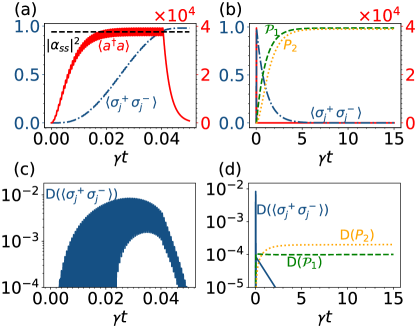
Figure 2: Synchronization of two deterministic SPSs via a cavity. (a) Short time dynamics: The cavity pulse is switched on $(f(t)=1)$ and a large coherent state with $\langle a^{\dagger}a\rangle\sim|\alpha_{\rm ss}|^{2}\sim 10^{4}$ photons is quickly created in the cavity with fast residual oscillations due to non-RWA terms [cf. red solid and black dashed lines]. This induces a cavity-mediated driving $\Omega_{\rm cm}=|\alpha_{\rm ss}|g$, which resonantly excites both qubits $\langle\sigma_{j}^{+}\sigma_{j}^{-}\rangle$ synchronously [cf. blue dash-dotted line]. After a $\pi$-pulse time $T\sim\pi/(2\Omega_{\rm cm})$, the cavity pulse is switched off $(f(t)=0)$, $\langle a^{\dagger}a\rangle$ decays in a fast timescale $\sim 1/\kappa$, and both qubits are left in their excited states $\langle\sigma_{j}^{+}\sigma_{j}^{-}\rangle\approx 1$. (b) Long time dynamics: Both qubits spontaneously decay in a timescale $t\sim 15/\gamma$, and each of them generates a single-photon with probability ${\cal P}_{1}\approx 0.99$ on its own antenna [cf.  green dashed line]. Since these spontaneous emission processes are much faster than the timescale for the cavity-mediated interactions ($J_{\rm cm}/\gamma\sim 10^{-5}$) and collective decay ($\gamma_{\rm cm}/\gamma\sim 10^{-4}$), both single-photons are nearly perfectly synchronized and independent as manifested by the two-photon probability satisfying $P_{2}\approx({\cal P}_{1})^{2}\approx 0.98$ [cf. yellow dotted line]. (c)-(d) Deviations $D(x)=|x_{\rm exact}-x_{\rm eff}|$ between the exact (6) and effective (12) models for the qubit occupations $x=\langle\sigma_{j}^{+}\sigma_{j}^{-}\rangle$, and photon generation probabilities $x={\cal P}_{1},P_{2}$ as a function of time. We observe great agreement and no heating effects despite the large cavity driving strength $\Omega_{0}=4\omega_{d}\gg\kappa,|\Delta|$. These and the rest of the parameters correspond to a state-of-the-art circuit-QED implementation shown in row C of Table 1 and discussed in Sec. III.1.

$\frac{\gamma}{2\pi}[{\rm MHz}]$

$\frac{\gamma_{\rm loss}}{2\pi}[{\rm kHz}]$

$\frac{\gamma_{\phi}}{2\pi}[{\rm kHz}]$

$\gamma/\Omega_{\rm cm}$

$\gamma_{\phi}/\gamma$

$\gamma_{\rm loss}/\gamma$

$\gamma_{\rm cm}/\gamma$

$J_{\rm cm}/\gamma$

${\cal P}_{1}$

$P_{2}$

$g^{(2)}_{\rm HBT}[0]$

$g^{(2)}_{\rm HOM}[0]$

A

0.4

0

0

$1.0\cdot 10^{-2}$

0

0

$9.4\cdot 10^{-4}$

$1.2\cdot 10^{-4}$

0.997

0.994

$4.4\cdot 10^{-3}$

$2.0\cdot 10^{-5}$

B

0.4

1

1

$1.0\cdot 10^{-2}$

$2.5\cdot 10^{-3}$

$2.5\cdot 10^{-3}$

$9.4\cdot 10^{-4}$

$1.2\cdot 10^{-4}$

0.994

0.989

$4.4\cdot 10^{-3}$

$2.5\cdot 10^{-3}$

C

1.0

5

10

$2.6\cdot 10^{-2}$

$1.0\cdot 10^{-2}$

$5.0\cdot 10^{-3}$

$3.8\cdot 10^{-4}$

$4.7\cdot 10^{-5}$

0.989

0.979

$1.0\cdot 10^{-2}$

$9.7\cdot 10^{-3}$

D

3.0

50

100

$7.7\cdot 10^{-2}$

$3.3\cdot 10^{-2}$

$1.7\cdot 10^{-2}$

$1.3\cdot 10^{-4}$

$1.6\cdot 10^{-5}$

0.968

0.936

$3.0\cdot 10^{-2}$

$3.1\cdot 10^{-2}$

Table 1: Parameters and figures of merit for a circuit-QED implementation of two synchronized SPSs. We study four parameter sets: A, B, C, and D, which show increasing antenna coupling $\gamma$ and decoherence rates $\gamma_{\rm loss}$, $\gamma_{\phi}$. The rest of the parameters are common to all sets and read $g/2\pi=0.2{\rm MHz}$, $\kappa/2\pi=400{\rm MHz}$, $\Delta/2\pi=50{\rm MHz}$, and $\Omega_{0}/2\pi=40{\rm GHz}$, which leads to $|\alpha_{\rm ss}|^{2}\approx 3.8\cdot 10^{4}$ photons in the cavity on average. The detuning of the qubits is chosen to compensate for the cavity-induced Lamb-shift $\delta_{q}=\delta_{\rm cm}$. Depending on the decoherence rates of sets A-D, the inequalities in Eq. (18) are satisfied differently, as shown in columns 5th to 9th, and this influences the performance of the four figures of merit: single-photon generation probability ${\cal P}_{1}$ [cf. Sec. III.2], synchronized two-photon generation efficiency or probability $P_{2}\approx({\cal P}_{1})^{2}$ [cf. Sec. III.3], multi-photon contamination $g^{(2)}_{\rm HBT}[0]$ [cf. Sec. III.4], and photon distinguishability $g^{(2)}_{\rm HOM}[0]$ [cf. Sec. III.5]. All these quantities are calculated using the full master equation (6), the methods in Appendices B.1 and C, and evolving up to a final time $t=15/\gamma$.

Fig. 2(a)-(b) illustrates the two processes in the cavity-mediated synchronization method, using two synchronized SPSs with parameters that satisfy Eq. (18). Fig. 2(a) displays the short time dynamics: the creation of a large coherent state on the cavity $\langle a^{\dagger}a\rangle\sim|\alpha_{\rm ss}|^{2}\sim 10^{4}$ [cf. red solid line], and the cavity-mediated simultaneous excitation of the qubits $\langle\sigma_{j}^{+}\sigma_{j}^{-}\rangle\approx 1$ [cf. blue dash-dotted line]. Fig. 2(b) shows the long time dynamics, in which the photons are generated. Each emitter decays almost independently in a timescale $t\sim 15/\gamma$, depositing a photon into its own antenna [cf. blue dash-dotted line]. To quantify the efficiency of these emission processes, we display the single-photon and synchronized two-photon generation probabilities, ${\cal P}_{1}$ and $P_{2}$, calculated using the definitions and methods in Secs. III.2-III.3. For non-optimized parameters satisfying Eq. (18), we reach ${\cal P}_{1}\approx 0.99$ [cf. green dashed line] and $P_{2}\approx({\cal P}_{1})^{2}\approx 0.98$ [cf. yellow dotted line]. This demonstrates that both emitted photons are highly independent between each other [$S_{2}\approx 1$ in Eq. (2)] and that cavity-induced correlations are indeed negligible during photon emission processes ($J_{\rm cm}/\gamma\sim 10^{-5}$ and $\gamma_{\rm cm}/\gamma\sim 10^{-4}$).

We performed the numerical simulations in Figs. 2(a)-(b) using both the full model in Eqs. (4)-(6) and the effective model in Eqs. (12)-(17). They show an excellent agreement with deviations $D(x)=|x_{\rm exact}-x_{\rm eff}|<10^{-2}$ in the qubit and photon counting observables [cf. Fig. 2(c)-(d)], despite the large cavity population of $\langle a^{\dagger}a\rangle\sim 10^{4}\gg 1$. This demonstrates that the strong cavity driving $\Omega_{0}\gg\kappa,|\Delta|$ does not introduce heating in the system, but only creates a large coherent state in the cavity with some fast oscillations around the mean value $|\alpha_{\rm ss}|^{2}\gg 1$ [cf. solid red and dashed black lines in Fig. 2(a)]. Since this fast oscillations have no detrimental impact in the functionality of our multiphoton generation scheme, in the remainder of the paper we use the simpler effective model (12) which uses the mean steady value (9) for describing the effect of the cavity field (see App. A for more details on the approximations involved in the model).

III Performance of a circuit-QED implementation

In this section, we describe typical state-of-the-art parameters to realize the synchronized multiphoton emitter in a circuit-QED implementation [cf. Sec. III.1]. Subsequently, we quantify the performance of the scheme using four figures of merit: (i) efficiency of single-photon generation ${\cal P}_{1}$ [cf. Sec. III.2], (ii) efficiency of synchronized $N$-photon generation $P_{N}$ [cf. Sec. III.3], (iii) single-photon purity as quantified by HBT correlations, $p=1-g^{(2)}_{\rm HBT}[0]$ [cf. Sec. III.4], and (iv) photon indistinguishability as quantified by HOM interference, $I=1-g^{(2)}_{\rm HOM}[0]$ [cf. Sec. III.5].

III.1 State-of-the-art parameters

In Fig. 1(b) we sketch a possible setup to implement the synchronized multiphoton emitter using superconducting circuits. For the cavity mode $a$, we consider a superconducting transmission line resonator with high decay rate $\kappa/2\pi=400{\rm MHz}$, and resonance frequency $\omega_{c}$ on the order of a few GHz. These superconducting resonators support strong drives and can hold a large number of photons in steady state $|\alpha_{\rm ss}|^{2}\gg 1$ Pietikäinen et al. (2017); Jenkins et al. (2014); Macrì et al. (2020), as it is required in our scheme. For this, we consider a driving with strength $\Omega_{0}/2\pi=40{\rm GHz}$, a detuning $\Delta/2\pi=50{\rm MHz}$, and an average number of photons $|\alpha_{\rm ss}|^{2}\approx 3.8\cdot 10^{4}$, well below the values $10^{5}-10^{9}$ photons observed in similar experiments Pietikäinen et al. (2017); Jenkins et al. (2014).

As two-level emitters, we consider flux-tunable transmon qubits DiCarlo et al. (2009); Barends et al. (2013); Pechal et al. (2014); Wang et al. (2020) weakly coupled to the resonator mode with strength $g/2\pi=0.2{\rm MHz}$. The cavity mediated driving amplitude is $\Omega_{\rm cm}/2\pi=|\alpha_{\rm ss}|g/2\pi\approx 39$MHz. This is strong but still smaller than typical transmon anharmonicities $U/2\pi\sim 300-400{\rm MHz}$ Pechal et al. (2014); McKay et al. (2019); Zhou et al. (2020), thus preventing leakage to higher excitation states. The frequency of the qubits—which will be on the few GHz range—can be fine-tuned by sending a DC current through the antenna that is coupled to each qubit [cf. Fig. 1(b)]. This is required to bring the qubits in resonance with the external drive, and to compensate the cavity-induced Lamb-shifts $\delta_{q}=\delta_{\rm cm}$ [See Sec. V for small deviations of this condition].

The antenna of each qubit is not only used for frequency calibration, but its main purpose is to collect the photons emitted by each qubit [cf. Fig. 1(b)]. The coupling rate between the qubit and antenna $\gamma$ can be chosen depending on the estimated decoherence parameters $\gamma_{\rm loss}$ and $\gamma_{\phi}$, so that the photons are efficiently ($\gamma\gg\gamma_{\rm loss}$) and coherently ($\gamma\gg\gamma_{\phi}$) collected. In our analysis, we consider four different combinations of the parameter sets ($\gamma,\gamma_{\rm loss}$,$\gamma_{\phi}$), shown in Table 1. Parameter set D corresponds to the typical relaxation $\gamma_{\rm loss}/2\pi\sim 50$kHz and dephasing rates $\gamma_{\phi}/2\pi\sim 100$kHz found in microwave quantum photonics experiments Pechal et al. (2014); Zhou et al. (2020); Wang et al. (2020). For this case we choose a relatively large decay rate of $\gamma/2\pi=3$MHz so that the emission time is faster than the decoherence timescales, but at the same time it is still slower than the effective driving $\Omega_{\rm cm}/2\pi\sim 39$MHz [cf. column D in Table 1]. In addition, parameter set C corresponds to decoherence rates reported in quantum computing experiments Barends et al. (2013); Caldwell et al. (2018); McKay et al. (2019); Andersen et al. (2020), which have reached relaxation and dephasing rates as low as $\gamma_{\rm loss}/2\pi\sim 5$kHz and $\gamma_{\phi}/2\pi\sim 10$kHz, respectively. For these parameters we can choose a slightly lower coupling to the antenna of $\gamma/2\pi\sim 1$MHz, and thus improve the ratio $\gamma/\Omega_{\rm cm}\sim 2.6\cdot 10^{-2}$ [cf. column C in Table 1]. Finally, set B corresponds to near-future parameters and set A to the ideal case of no decoherence, which we use as a reference to quantify the intrinsic limitations of the synchronization method. In the remainder of the paper, we use these four parameter sets A-D to characterize the performance and scaling of the synchronized SPSs for this circuit-QED implementation.

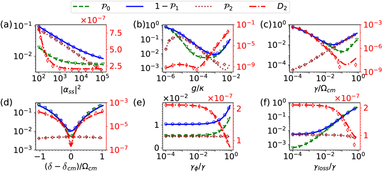
Figure 3: Few-photon statistics ${\cal P}_{n}$ and two-photon dependence $D_{2}$ as a function of various system parameters such as (a) cavity occupation $|\alpha_{\rm ss}|^{2}$, (b) qubit-cavity coupling $g/\kappa$, (c) qubit-antenna decay $\gamma/\Omega_{\rm cm}$, (d) qubit-drive detuning $(\delta-\delta_{\rm cm})/\Omega_{\rm cm}$, (e) dephasing $\gamma_{\phi}/\gamma$, and (f) relaxation loss $\gamma_{\rm loss}/\gamma$. The probabilities ${\cal P}_{0}$ (green), $1-{\cal P}_{1}$ (blue), and ${\cal P}_{2}$ (brown) are plotted using the left vertical axis, whereas the two-photon dependence $D_{2}$ (red), corresponds the right vertical axis. Solid lines are computed using the effective master equation in Eq. (12) and the discrete symbols using the full master equation in Eq. (6), which show excellent agreement. Parameters are given by set C of Table 1, except for the quantity that is changed on each subplot.

III.2 Efficiency of single-photon generation

Without loss of generality, in our discussion about photon generation efficiencies or probabilities, we assume perfect photo-detectors . In this scenario, the efficiency of a single photon source can be extracted from the photon emission statistics. For a single emitter, ${\cal P}_{1}$ is the probability of generating exactly an isolated photon in a Fock state Senellart et al. (2017). Similarly, we define ${\cal P}_{n}^{j}$ as the probability for the synchronized SPS to emit a Fock state of $n$ photons in the $j$-th antenna. Formally,

$${\cal P}_{n}^{j}={\rm Tr}\{\Lambda_{n}^{j}\rho_{\rm ext}(t)\},$$ (19)

where $\rho_{\rm ext}(t)$ is the state of the extended system including the photons emitted in all antennas. The operator $\Lambda_{n}^{j}=|n\rangle_{j}\langle n|$ projects $\rho_{\rm ext}(t)$ on the Fock state $|n\rangle_{j}$ of $n$ photons propagating in the independent antenna $j$. Computing ${\cal P}_{1}$ or ${\cal P}_{n}^{j}$ seems to require a large Hilbert space, but there are shortcuts, such as the quantum jump formalism or our new photon counting approach based on master equations [cf. App. B].

A nearly deterministic single-photon source should have ${\cal P}_{1}\approx 1$, other few-photon probabilities ${\cal P}_{0}$ and ${\cal P}_{2}$ should be strongly suppressed, and ${\cal P}_{n\geq 3}\approx 0$ negligible. This also applies to each of the probabilities ${\cal P}_{n}^{j}$ in our synchronized setup, if we want it to operate as a collection of $N$ independent emitters.

To verify this, we have computed the few-photon probabilities ${\cal P}_{0}$ (green), $1-{\cal P}_{1}$ (blue), and ${\cal P}_{2}$ (brown) for a setup with $N=2$ superconducting qubits, varying different parameters around the set C from Table 1. The results in Figs. 3(a)-(f), have been computed using the full model (6) and the effective equation (12), and are shown in lines and markers, respectively. The agreement between both methods confirms that the adiabatic elimination of the cavity is an excellent approximation over a broad range of parameters.

In Fig. 3(a) we plot the effect of cavity occupation $|\alpha_{\rm ss}|^{2}$ (controlled via the cavity drive $\Omega_{0}$) on the single-photon efficiency of the SPS. All errors reduce with the cavity population $|\alpha_{\rm ss}|^{2},$ because a larger cavity-mediated driving $\Omega_{\rm cm}=|\alpha_{\rm ss}|g$ increases the speed at which the qubit is excited and reduces the probability of emitting two consecutive photons. However, the driving strength is limited by our need to have an off-resonant cavity and by the anharmonicity of the qubits [cf. Sec. III.1].

Fig. 3(b) illustrates the need to find an optimum value of the coupling $g$, within inequalities in Eq. (18). Initially, increasing $g$ increases the driving $\Omega_{\rm cm}$ and reduces errors. However, a large coupling strength enhances the cavity-mediated dipole-dipole interactions $J_{\rm cm}\sim g^{2}$ and the collective decay $\gamma_{\rm cm}\sim g^{2}$. Both result in the transfer of excitations between qubits, increasing the probability of no emission ${\cal P}_{0}$ and of two photon emission ${\cal P}_{2}.$ For the parameters in Table 1 we find an optimal operation point around $g/\kappa=4\cdot 10^{-4}$.

In Fig. 3(c) we analyze the effect of the coupling to the antenna coupling $\gamma.$ Once more, there is an optimal point that satisfies (18), balancing the imperfections due to unwanted re-excitations ($\Omega_{\rm cm}\gg\gamma$) and cavity-mediated effects ($\gamma\ll J_{\rm cm},\gamma_{\rm cm}$). The optimal lays around $\gamma/\Omega_{\rm cm}\sim 2\cdot 10^{-2}$ for the parameter set C in Table 1.

Fig. 3(d) clearly shows an optimal operation of the emitters when they are on resonance with the drive $\delta=\delta_{\rm cm}$. At this point, a $\pi$ pulse excites the qubits with high fidelity, and the Lamb-shift is compensated.

Finally, in Fig. 3(e) and Fig. 3(f), we observe that the dephasing $\gamma_{\phi}$ and the losses into uncontrolled channels $\gamma_{\rm loss}$ have a negligible influence on the few-photon statistics ${\cal P}_{n}$ as long as they satisfy $\gamma_{\phi},\gamma_{\rm loss}\ll\gamma$ [cf. Eq. (18)]. Nevertheless, when $\gamma_{\phi},\gamma_{\rm loss}\sim\gamma$ we see a rapid increase of events where no photon is detected ${\cal P}_{0}.$ This is due to emitters becoming effectively off-resonant from the drive when $\gamma_{\phi}\sim\gamma$, or due to a decrease in the the collection efficiency in the antenna, when $\gamma_{\rm loss}\sim\gamma.$

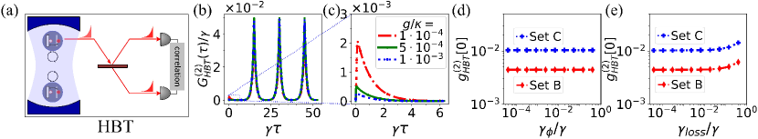
Figure 4: Multi-photon contamination of the SPS measured via the second-order correlation function. (a) Schematic of the Hanbury Brown and Twiss (HBT) experiment using a beam-splitter (BS) and two-photon coincidence measurements. (b) HBT correlation function $G^{(2)}_{\rm HBT}(\tau)$ as a function of delay $\tau$, in the case of a train of 4 excitation pulses with repetition rate $R=\gamma/15$. Parameters correspond to set C of Table 1. (c) Enlarged plot of $G^{(2)}_{\rm HBT}(\tau)$ at the zeroth peak, $\tau\sim 0$, for three values of couplings $g/\kappa=[1,5,10]\cdot 10^{-4}$. (d,e) Normalized correlation function $g^{(2)}_{\rm HBT}[0]$ at zero delay, as function of dephasing $\gamma_{\phi}/\gamma$ and out-coupling inefficiency $\gamma_{\rm loss}/\gamma$, respectively. Other parameters correspond to set C (blue) and set B (red). Decoherence has a small detrimental effect on the observed multi-photon contamitation via $g^{(2)}_{\rm HBT}[0]$.

III.3 Efficiency of synchronized N-photon generation

The quantity ${\cal P}_{1}$ is the probability of generating one photon on a given antenna irrespective of the photons emitted in the rest of the channels. To study SPS synchronization, however, we are interested in the probability $P_{N}$ of emitting exactly one photon on each of the $N$ available antennas or channels. This can be expressed using projectors onto single-photon Fock states $\Lambda_{1}^{j}=|1\rangle_{j}\langle 1|$ on each the channels

$$P_{N}={\rm Tr}\{\Lambda_{1}^{1}\cdots\Lambda_{1}^{N}\rho_{\rm ext}(t)\},$$ (20)

An efficient generation of $N$ synchronized and independent single-photons should satisfy $P_{N}\approx({\cal P}_{1})^{N}\leq{\cal P}_{1}$, meaning that the $N$-photon product state (1) is generated with high fidelity. This happens for all parameter sets in Table 1. The two-photon generation probability satisfies $P_{2}\approx({\cal P}_{1})^{2}\lesssim 1,$ and deviates from unity because of errors in the single-photon efficiency ${\cal P}_{1}\lesssim 1$.

To quantify more precisely the independence of the $N$ emitted photons, we define the $N$-photon dependence or demultiplexing error as,

$$D_{N}=\frac{P_{N}}{({\cal P}_{1})^{N}}-1,$$ (21)

which describes the deviation from the ideal limit of $N$ perfectly independent and synchronized SPSs. This quantity is also related to the demultiplexing inefficiency in Eq. (2) as $S_{N}=1+D_{N}$.

We have computed $P_{N}$ and $D_{N}$ in the simplest case of two SPSs, using the same photon counting methods introduced in Appendix B. The results of these simulations are shown as red curves of Figs. 3(a)-(f) [cf. red curves and right vertical axis]. We observe that $D_{2}$ is nearly insensitive to changes in the cavity occupation $|\alpha_{\rm ss}|^{2}$, the dephasing $\gamma_{\phi}/\gamma$, and out-coupling efficiency $\gamma_{\rm loss}/\gamma$, with typical values on order $D_{2}\sim 10^{-7}$ for parameters around set C of Table 1. Nevertheless, the variables $g$, $\gamma$, and $\delta$ can drastically change $D_{2}$ in various orders of magnitude. In particular, for larger cavity coupling $g$ or smaller antenna decay $\gamma$, $D_{2}$ increases because the cavity-mediated correlations $\sim g^{2}$ become more important in the timescale of the photon emission $\sim 15/\gamma$ [cf. right inequality in Eq. (18)].

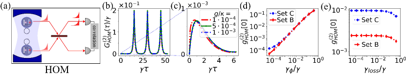
Figure 5: Indistinguishability of single-photons from two different SPSs quantified by Hong-Ou-Mandel (HOM) interference. (a) Schematic of the HOM setup using a beam splitter to interfere two nearly independent photons, followed by two-photon coincidence measurements. (b) HOM correlation function $G^{(2)}_{\rm HOM}(\tau)$ as a function of delay $\tau$, in the case of a train of 4 excitation pulses with repetition rate $R=\gamma/15$. Parameters correspond to set C of Table 1. (c) Enlarged plot of $G^{(2)}_{\rm HOM}(\tau)$ at the zeroth peak, $\tau\sim 0$, for three values of couplings $g/\kappa=[1,5,10]\cdot 10^{-4}$. (d,e) Normalized correlation function $g^{(2)}_{\rm HOM}[0]$ at zero delay, as function of dephasing $\gamma_{\phi}/\gamma$ and out-coupling inefficiency $\gamma_{\rm loss}/\gamma$, respectively. Other parameters correspond to set C (blue) and set B (red). The indistinguishability dramatically reduces with dephasing, a behaviour in good agreement with the analytical prediction $g^{(2)}_{\rm HOM}[0]\approx(\gamma_{\phi}/\gamma)/(1+\gamma_{\phi}/\gamma)$ Bylander et al. (2003).

Finally, we note that the exact pulse shape $f(t)$ is not relevant for the synchronization dynamics as long as it approximately induces a $\pi$-pulse on the qubits. To study this, we have performed the calculations in Figs. 3(a)-(f) using an ideal square pulse and a smooth step pulse $f(t)=\frac{1}{2}\tanh(\frac{t}{\tau_{r}})\{2-\tanh(\frac{T}{\tau_{r}})-\tanh(\frac{t-T}{\tau_{r}})\}$ with duration $T$ and ramp time $\tau_{r}$. When optimizing over $T$ and $\tau_{r}$ of the smooth pulse, we obtain a deviation smaller than $1\%$ with respect to the result of the simpler square $\pi$-pulse with $T=\pi/(2\Omega_{\rm cm})$. Therefore, in the remainder of the paper we safely consider the ideal square pulse, but we keep in mind that a realistic experimental pulse shape gives similar results when properly optimized.

III.4 Single-photon purity

A standard figure of merit to experimentally quantify the amount of multi-photon contamination of a SPS is the second-order correlation function $G_{\rm HBT}^{(2)}$ Kiraz et al. (2004); Fischer et al. (2016). As sketched in Fig. 4(a), this is measured in a Hanbury Brown and Twiss (HBT) setup, where the output of a given SPS is beam-splitted and measured via coincidences in two intensity detectors. For pulsed emission, the correlation function $G_{\rm HBT}^{(2)}(\tau)$ is defined as Kiraz et al. (2004); Fischer et al. (2016)

$$G_{\rm HBT}^{(2)}(\tau)\!=\! \int\!\mathrm{d}t\,\langle b^{j{\dagger}}_{\rm out}(t)b^{j{\dagger}}_{\rm out}(t+\tau)b^{j}_{\rm out}(t+\tau)b^{j}_{\rm out}(t)\rangle,$$ (22)

where $\tau$ is the time delay between the two photon detections, and $b^{j}_{\rm out}(t)$ is the annihilation operator for an outgoing photon on the $j$-th antenna Gardiner and Zoller (2004). Appendix C contains details on the input-output theory and the calculation of these correlations. For simplicity, our analysis assumes a homogeneous setup and thus we omit the $j$ index in $G_{\rm HBT}^{(2)}(\tau)$.

In Fig. 4(b) we show the behaviour of the correlation $G_{\rm HBT}^{(2)}(\tau)$ in our setup for train of 4 excitation pulses with a repetition rate

$$R=\gamma/15.$$ (23)

We observe clear peaks at integer multiples of the repetition time $\tau=n/R$, corresponding to the detection of two photons coming from different pulses. Relevant to characterize the few-photon statistics of the SPS is the small peak that appears near zero time delay, $\tau\sim 0.$ A small area in this peak signals a small probability of two- and multi-photon emission Kiraz et al. (2004). In Fig. 4(c) we enlarge the region $\tau\sim 0$ and show that the area of the zeroth peak increases with $g/\kappa,$ consistently with the behavior of ${\cal P}_{2}$ in Fig. 3(b) for the same parameters.

To quantify more precisely the amount of multi-photon contamination of the SPS, and in a way that is independent of the input power, it is convenient to define the normalized correlation $g_{\rm HBT}^{(2)}[0]$ at zero delay as Fischer et al. (2016)

$$g_{\rm HBT}^{(2)}[0]=\frac{\int_{0}^{1/(2R)}d\tau G_{\rm HBT}^{(2)}(\tau)}{\left(\int_{0}^{1/(2R)}dt\langle b_{\rm out}^{j{\dagger}}(t)b_{\rm out}^{j}(t)\rangle\right)^{2}}.$$ (24)

Here, the numerator corresponds to the area of the zeroth peak at $\tau\sim 0$ and the normalization is the area of one of the high peaks at $\tau\sim n/R$, and thus $g_{\rm HBT}^{(2)}[0]\sim{\cal P}_{2}/({\cal P}_{1})^{2}$. In Figs. 4(d)-(e), we plot the normalized correlation $g_{\rm HBT}^{(2)}[0]$ as a function of $\gamma_{\phi}/\gamma$ and $\gamma_{\rm loss}/\gamma$, respectively. We observe that $g_{\rm HBT}^{(2)}[0]$ is very insensitive to both types of decoherence, which is also consistent to the behaviour of ${\cal P}_{2}$ in Fig. 3(e)-(f) for the same parameters. In addition, we see that parameter set B gives a two-photon contamination of $g_{\rm HBT}^{(2)}[0]\sim 2.5\cdot 10^{-3}$, slightly lower than parameter set C [cf. Fig. 4(e)-(f) and Table 1]. Finally, we note that the single-photon purity $p$ is sometimes defined as $p=1-g_{\rm HBT}^{(2)}[0]$, which for parameter sets B and C of our circuit-QED implementation is higher than $p=0.99$.

III.5 Indistinguishability

Another important aspect of a high-performance multiphoton demultiplexing scheme is the degree of indistiguishability of the photons emitted by two different sources Senellart et al. (2017). Experimentally, the distinguishability of two sources is typically quantified using Hong-Ou-Mandel (HOM) interference as shown in Fig. 5(a). Photons coming from two sources interfere on a beam-splitter (BS), and a pair of detectors count coincidences. The result of these measurements are the HOM correlations $G_{\rm HOM}^{(2)}(\tau)$, which for pulsed emission read Fischer et al. (2016)

$$G_{\rm HOM}^{(2)}(\tau)\!=\!\int dt\langle b_{\text{BS}}^{1{\dagger}}(t)b_{BS}^{2{\dagger}}(t+\tau)b_{BS}^{2}(t+\tau)b_{BS}^{1}(t)\rangle,$$ (25)

where $\tau$ is the delay time between the two photon detections. In addition, $b_{BS}^{1}(t)=[b^{1}_{\rm out}(t)+b^{2}_{\rm out}(t)]/\sqrt{2}$, and $b_{BS}^{2}(t)=[b^{1}_{\rm out}(t)-b^{2}_{\rm out}(t)]/\sqrt{2}$, describe the output fields of photons after interfering at the BS [cf. Appendix C].

Due to the bosonic nature of the emitted photons, two perfectly indistinguishable photons will bunch on either output port of the BS, resulting in a vanishing HOM correlation $G_{\rm HOM}^{(2)}(\tau)$ at zero time delay $\tau\sim 0$. This is perfect HOM interference, and any deviation from it (assuming an ideal BS) can be used to quantify the distinguishability of the generated single-photons.

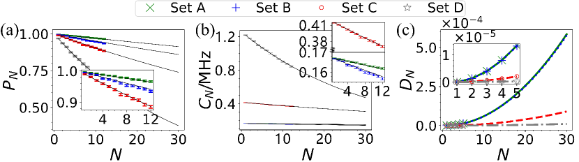
Figure 6: Scalability performance of the synchronized multiphoton generation scheme. (a) $N$-photon generation efficiency $P_{N}$ as a function of $N$, for parameter sets A (green), B (blue), C (red), and D (grey), as given in Table 1. Data points up to $N=12$ correspond to QT calculations averaged over $M=6000$ trajectories, which show excellent agreement (within the statistical error $\Delta P_{N}\sim 10^{-3}$) with the prediction for perfectly independent and synchronized SPSs, i.e. $P_{N}\approx({\cal P}_{1})^{N}$. [cf. black lines and inset]. (b) $N$-photon generation rate $C_{N}=RP_{N}$ for pulsed excitation with repetition rate $R=\gamma/15$. Despite parameter set D shows the lowest $P_{N}$ efficiency, its faster repetition rate $R\sim 1.2$MHz allows for appreciably higher $C_{N}$. (c) Demultiplexing error $D_{N}$ up to $N=5$, and quadratic fit $D_{N}=\epsilon N(N-1)$ (cf. solid lines and inset). The fitted scaling factor depends on the system parameters [cf. Eq. (28)] and read $\epsilon_{A}=6.7\times 10^{-7}$, $\epsilon_{B}=6.7\times 10^{-7},\epsilon_{C}=1.0\times 10^{-7}$, and $\epsilon_{D}=1.3\times 10^{-8}$ for parameter sets A, B, C, and D, respectively. The extrapolation of all these calculations are valid as long as $D_{N}\lesssim 1$.

A standard figure of merit of indistinguishability that accounts for losses and other imperfections is the normalized HOM correlation function $g_{\rm HOM}^{(2)}[0]$ Fischer et al. (2016)

$$g_{\rm HOM}^{(2)}[0]=\frac{\int_{0}^{1/(2R)}d\tau G_{\rm HOM}^{(2)}(\tau)}{\prod_{k=1}^{2}\left(\int_{0}^{1/(2R)}dt\langle b_{BS}^{k{\dagger}}(t)b_{BS}^{k}(t)\rangle\right)}.$$ (26)

In analogy to Eq. (24), the numerator of Eq. (26) corresponds to the area below the zeroth peak and the normalization to the area of one of the high peaks at the repetition times $\tau=n/R$. The indistinguishability of two SPSs can be simply defined as $I=1-g^{(2)}_{\rm HOM}[0].$

We have computed $G_{\rm HOM}^{(2)}(\tau)$ as a function of $\tau$, for a setup with two emitters and a train of 4 excitation pulses [cf. Fig. 5(b)]. Here, we observe clear peaks at the repetition times $\tau=n/R$ due to the detection of two nearly independent photons coming from two different pulses. The correlations $G_{\rm HOM}^{(2)}(\tau)$ are strongly suppressed at the origin, $\tau\sim 0$, showing only a minor zeroth peak which is enlarged in Fig. 5(c). The small area of this zeroth peak manifests the high indistinguishability of the single-photons prepared in our setup with parameter set C. We also see that this behaviour is nearly insensitive to the coupling $g/\kappa$, but may strongly depend on the decoherence parameters.

Figures 5(d)-(e) display $g^{(2)}_{\rm HOM}[0]$ as function of the decoherence rates $\gamma_{\phi}/\gamma$ and $\gamma_{\rm loss}/\gamma.$ Note that in our implementation with parameters B and C we reach values above $I=0.99$, as inferred from Fig. 5(e) and Table 1. We also find that the distinguishability $g^{(2)}_{\rm HOM}[0]$ is quite insensitive to $\gamma_{\rm loss}/\gamma$, but it dramatically increases with dephasing, following the analytical prediction $g^{(2)}_{\rm HOM}[0]\approx(\gamma_{\phi}/\gamma)/(1+\gamma_{\phi}/\gamma)$ Bylander et al. (2003). This contrasts with the behaviour of $D_{2}$ in Fig. 3(e), illustrating that the dependence error $D_{2}$ of two SPSs is qualitatively different from the distinguishability $g^{(2)}_{\rm HOM}[0]$ measured by HOM interference. Consequently, both figures of merit have to be considered when designing high-performance multiplexed and synchronized SPSs.

IV Scalability of synchronized multiphoton generation

We are now in position to discuss the most important results of the present work: the scalability performance of the multiphoton emitter. To do so, we analyze the $N$-photon generation probability $P_{N}$ and the demultiplexing error $D_{N}$ as a function of $N$ and the various system parameters. From these results we demonstrate the feasibility to synchronize $N\sim 100-1000$ emitters with high $N$-photon generation rates $C_{N}=RP_{N}$.

We calculate $P_{N}$ in Eq. (20) by solving the master equation (12), which includes all qubit-qubit correlations induced by the cavity ($\sim J_{\rm cm},\gamma_{\rm cm}$), as well as the decoherence effects ($\sim\gamma_{\phi},\gamma_{\rm loss}$). The Hilbert space of the system grows exponentially as $2^{N}$, but using quantum trajectories (QT) [cf. Appendix B.2] we can estimate the photon statistics of the multiphoton emission and thereby $P_{N}$ up to moderately large numbers of SPSs. Figure. 6(a) displays $P_{N}$ as a function of $N$ computed from an average over $M=6000$ trajectories and considering the four parameter sets of Table 1. In the four cases and up to $N=12$, we numerically confirm that the SPSs are nearly perfectly synchronized and independent, satisfying $P_{N}\approx({\cal P}_{1})^{N}$ within the the statistical error $\Delta P_{N}\sim 10^{-3}$ [cf. black lines in Fig. (6)]. The reduction of $N$-photon generation probability with $N$ is thus mainly limited by the imperfections in the single-photon efficiency ${\cal P}_{1}$ and not by the synchronizing and demultiplexing scheme. For the decoherence-free parameters A, we predict a $12$-photon efficiency as high as $P_{12}\approx 0.97$, and when including realistic decoherence sources as in parameter set C [cf. inset in Fig. 6(a)], this reduces only to $P_{12}\approx 0.88$. For a pulsed excitation of the SPSs with a repetition rate $R=\gamma/15$ (as in Secs. III.4-III.5), these high efficiencies imply $12$-photon generation rates $C_{12}=RP_{12}$ of $\sim 0.1-1$MHz [cf. Fig. 6(b) and inset]. Since parameter set D has the largest antenna decay $\gamma/2\pi\sim 3$MHz, it shows the largest $N$-photon generation rates $C_{N}$ despite having the lowest efficiencies $P_{N}$ and the largest decoherence rates.

To quantify more precisely the deviations from the ideal scaling $P_{N}\approx({\cal P}_{1})^{N}$ in Figs. 6(a)-(b), we compute the $N$-photon dependence or demultiplexing error $D_{N}$ as defined in Eq. (21). For $N=2$ we know this error is as small as $D_{2}\sim 10^{-7}$ [cf. Figs. 3] and therefore the QT calculations with an uncertainty $\Delta P_{N}\sim 10^{-3}$ do not provide enough precision. To address this problem, we developed a photon counting approach based on the master equation [cf. Appendix B.1], which does not suffer from any statistical uncertainty. In this alternative method we simulate the photon counters at each antenna by an additional two-level system. This increases the Hilbert space dimension to $2^{2N}$ and thus limits the numerical computations to a maximum of $N\sim 5$ emitters.

In the inset of Fig. 6(c) we show the results of $D_{N}$ as a function $N$ for the four parameter sets of Table 1, and up to $N=5$. We confirm that $D_{N}<10^{-5}$ is well below the QT precision, and most importantly, we observe that the data is very well approximated by the quadratic fit

$$D_{N}=\epsilon N(N-1),$$ (27)

where the scaling factor $\epsilon\ll 1$ depends on the system parameters [cf. inset of Fig. 6(c)]. To analyze how the cavity-induced correlations influence $\epsilon$ and thus the scalability of the multiphoton scheme, we vary the system parameters around parameter set B and extract $\epsilon$ from fits to numerical calculations of $D_{N}$ up to $N=5$. The results of this analysis are represented by the data points in Fig. 7(a), which correspond to independent sweeps over each of the system parameters. Remarkably, the apparently complicated behaviour of the system is very well approximated by the analytical formula [cf. solid lines in Fig. 7(a)],

$$\epsilon\approx(1.42)\frac{g^{4}}{\gamma^{2}}\frac{\kappa}{\left[(\kappa/2)^{2}+\Delta^{2}\right]^{3/2}},$$ (28)

which manifests the dominant dependence on $g$, $\gamma$, $\kappa$, and $\Delta$, and omits the marginal effects of the effective driving $\Omega_{\rm cm}$, and the decoherence rates $\gamma_{\rm loss}$ and $\gamma_{\phi}$. This confirms our intuition that the synchronization and demultiplexing performance of our scheme is limited exclusively by residual cavity-induced correlations, provided $J_{\rm cm},\gamma_{\rm cm}\ll\gamma$ [cf. Eq. (18)].

Although Eq. (28) was extracted from a variation of parameters around set B of Table 1, this expression accurately predicts the scaling factors $\epsilon$ obtained from the fits on all parameters sets A-D in Fig. 6(c) with an error smaller than $8\%$. Interestingly, we can exploit Eq. (28) to predict new parameter sets whose demultiplexing error grows quickly to $D_{N}\gtrsim 1$ for moderate system sizes $N\lesssim 10$. Setups with these characteristics can then be used to study the validity limits of the approximated $D_{N}$ scaling in Eq. (27). In Fig. 7(b) we illustrate this analysis by calculating $D_{N}$ for two parameter sets similar to B, but: (i) with a $10$-fold coupling enhancement $g/2\pi=2$MHz (blue data), and (ii) with a $1/2$ reduction of decay $\gamma/2\pi=0.2$MHz in addition to the same $10$-fold increase in $g$ (red data). We perform $D_{N}=\epsilon N(N-1)$ fits to both data sets up to $N=5$, and we clearly observe the on-set of deviations from this scaling only when $D_{N}\gtrsim 1$ [cf. solid red line in Fig. 7]. For $D_{N}\ll 1$, both data sets show excellent agreement with the quadratic scaling (27), and this constitutes the range of validity of this approximation.

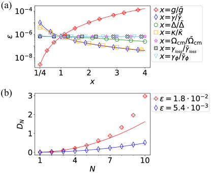
Figure 7: Limits on the scalability of the synchronized multiphoton generation. (a) Scaling factor $\epsilon$ as a function of various system parameters. The dimensionless variable $x=1$ corresponds to the parameters of set B in Table 1, which are denoted by $\tilde{g}$, $\tilde{\gamma}$, $\tilde{\Delta}$, $\tilde{\kappa}$, $\tilde{\Omega}_{\rm cm}$, $\tilde{\gamma}_{\rm loss}$, $\tilde{\gamma}_{\phi}$, and in this plot we change each of them from $25\%$ to $400\%$. We use these results to numerically extract Eq. (28). (b) Demultiplexing error $D_{N}$ calculated up to $N=10$ with QT averaged over $M=10^{4}$ trajectories. Both parameter sets are similar to B, except for $g/2\pi=2$MHz (blue data) and $[g/2\pi,\gamma/2\pi]=[2,0.2]$MHz (red data). Solid lines correspond to fits of $D_{N}=\epsilon N(N-1)$ up to $N=5$, which result in the $\epsilon$ factors shown in the legend. For both data sets we observe that the quadratic scaling is a good approximation as long as $D_{N}\ll 1$, confirming the expected limit of validity.

After analyzing the demultiplexing error $D_{N}$ as a function of $N$, and identifying the limits of scalability in the condition $D_{N}\ll 1$, we can safely extrapolate the results in Figs. 6(a)-(c) up to a large $N\gg 1$, only limited by $N\ll\epsilon^{-1/2}$. Since the scaling factors for parameters A-D of Table 1 are in the range $\epsilon\sim 10^{-8}-10^{-6}$ [cf. Fig. 6(c) and caption], we conclude that our multiphoton generation scheme allows for nearly perfect synchronization up to $N\sim 100-1000$ SPSs, depending on the decoherence rates. In particular, for the state-of-the-art circuit-QED parameters C, we therefore predict a 30-photon generation probability of $P_{30}\approx(0.989)^{30}\approx 0.72$, with a high generation rate of $C_{30}\sim 290$kHz [cf. solid black lines in Figs. 6(a)-(b)]. Following the same extrapolation, we also predict a 100-photon probability of $P_{100}\approx(0.989)^{100}\approx 0.33$ with a generation rate of $C_{100}=RP_{100}\sim 130$kHz. This is orders of magnitude more efficient than the $3$- to $14$-photon generation rates in the range $\sim$kHz-mHz that has been reported in recent boson sampling experiments Lenzini et al. (2017); Wang et al. (2017); Loredo et al. (2017); Wang et al. (2019a); Antón et al. (2019); Hummel et al. (2019).

V Inhomogeneity effects

So far, we have analyzed the performance of the scheme assuming a perfectly homogeneous setup. In large scale implementations, however, the SPS parameters will unavoidably present some degree of inhomogeneity. In this last section we analyze the impact of these imperfections.

We consider inhomogeneity deviations on all qubit parameters, which we generically denote by

$$y_{j}=y+\delta y_{j},$$ (29)

where $y=\omega_{q},g,\gamma,\gamma_{\phi},\gamma_{\rm loss}$ are the average qubit parameters discussed in the previous sections [cf. Table 1] and $\delta y_{j}$ are random deviations over each of them. To statistically describe each of these deviations $\delta y_{j}$, we assume that they are distributed according to a Gaussian probability distribution,

$$\Pi(\delta y_{j})=\frac{1}{\sqrt{2\pi(\Delta y)^{2}}}{\rm exp}\left(-\frac{1}{2}\left[\frac{\delta y_{j}}{\Delta y}\right]^{2}\right).$$ (30)

Here, $\Delta y$ denotes the standard deviation associated to the disorder on each qubit parameter $y=\omega_{q},g,\gamma,\gamma_{\phi},\gamma_{\rm loss}$.

To quantify the impact of each of the inhomogeneities $\delta y_{j}$ on the performance of the multiphoton emitter, we compute the average $N$-photon efficiency $\langle\!\langle P_{N}\rangle\!\rangle_{y}$ as

$$\langle\!\langle P_{N}\rangle\!\rangle_{y}=\frac{1}{M}\sum_{m=1}^{M}P_{N}[m]_{y},$$ (31)

where the probabilities $P_{N}[m]_{y}$ are calculated with the master equation method of Appendix B.1 for each realization $m=1,\dots,M$ of the independent disorder $y$. The results of these computations for $\langle\!\langle P_{N}\rangle\!\rangle_{y}$ in the case of disorder on the antenna couplings $\Delta\gamma$, as well as in the decoherence rates $\Delta\gamma_{\phi}$ and $\Delta\gamma_{\rm loss}$, are shown in Fig. (8). We perform calculations up to $N=4$ slightly inhomogeneous photon sources, for parameters B and C, and we do not observe any detrimental effect up to a disorder strength of $10\%$ of the average values [cf. Fig. 8(a)-(b)]. This is not surprising in the case of inhomogeneous decoherence rates $\gamma_{\phi}^{j}$ and $\gamma_{\rm loss}^{j}$ since their effects have nothing to do with the synchronization dynamics and are very marginally small anyways $\gamma_{\phi}^{j},\gamma_{\rm loss}^{j}\ll\gamma$. In the case of inhomogeneous antenna couplings $\gamma_{j}=\gamma+\delta\gamma_{j}$, they imply slightly different emission time scales for the emitted single-photons,

$$t\gg\frac{1}{\gamma+\delta\gamma_{j}}=\frac{1}{\gamma}\left(1-\frac{\delta\gamma_{j}}{\gamma}+{\cal O}^{2}\right),$$ (32)

but since we consider a long average waiting time $t=15/\gamma$, the effect of $10\%$ inhomogeneity in $\delta\gamma_{j}/\gamma$, is negligible on that timescale.

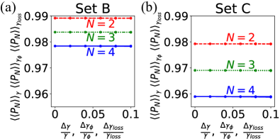
Figure 8: Average $N$-photon generation probabilities $\langle\!\langle P_{N}\rangle\!\rangle_{y}$, as a function of disorder in antenna decay $y=\Delta\gamma/\gamma$, qubit dephasing $y=\Delta\gamma_{\phi}/\gamma_{\phi}$, and waveguide loss $y=\Delta\gamma_{\rm loss}/\gamma_{\rm loss}$. (a)-(b) Up to a disorder strength of $10\%$, we do not observe any impact of these three disorder sources on the synchronization and demultiplexing dynamics, as calculated up to $N=4$ for parameter sets B and C, respectively. All results are obtained from averaging $M=10^{3}$ realizations for each type of disorder.

On the other hand, inhomogeneities in the qubit frequencies $\delta\omega^{j}_{q}$ and in the couplings $\delta g_{j}$ are much more harmful for the multiphoton synchronization performance and therefore they need to be controlled more precisely in an experimental implementation of the device. Inhomogeneous couplings $g_{j}$, in particular, induce different cavity-mediated driving strengths $\Omega^{j}_{\rm cm}=\Omega_{\rm cm}+|\alpha_{\rm ss}|\delta g_{j}$, and therefore different times to realize an exact $\pi$-pulse on each qubit $\sim\pi/(2\Omega_{\rm cm}^{j})$. Since we control only the global duration of the cavity pulse, we optimally set it to the average $\pi$-pulse time $T=\pi/(2\Omega_{\rm cm})$, but this unavoidably leads to slightly different probabilities $P_{e}^{j}$ of preparing the excited states $|e\rangle_{j}$ on each qubit. Explicitly, we have

$$P_{e}^{j}\approx\sin^{2}\left(\frac{\pi}{2}\frac{\Omega_{\rm cm}^{j}}{\Omega_{\rm cm}}\right)=1-\frac{\pi^{2}}{4}\left(\frac{\delta g_{j}}{g}\right)^{2}+{\cal O}^{4},$$ (33)

and therefore a low coupling disorder $\delta g_{j}\ll g$ is required for a high performance of the synchronized multiphoton emitter. To precisely quantity the deviation from the ideal photon independence condition, we define the average dependence or demultiplexing error $\langle\!\langle D_{N}\rangle\!\rangle_{y}$ over disorder $y$ as

$$\langle\!\langle D_{N}\rangle\!\rangle_{y}=\frac{\langle\!\langle P_{N}\rangle\!\rangle_{y}}{\left(\langle\!\langle{\cal P}_{1}\rangle\!\rangle_{y}\right)^{N}}-1.$$ (34)

Here, the average single-photon efficiency reads,

$$\langle\!\langle{\cal P}_{1}\rangle\!\rangle_{y}=\frac{1}{MN}\sum_{j=1}^{N}\sum_{m=1}^{M}{\cal P}_{1}^{j}[m]_{y},$$ (35)

with ${\cal P}_{1}^{j}[m]_{y}$ calculated from $m=1,\dots,M$ realizations of the disorder $y$ and for each of the $j=1,\dots,N$ SPSs in the setup. In Figs. 9(a)-(b) we compute $\langle\!\langle P_{N}\rangle\!\rangle_{g}$ and $\langle\!\langle D_{N}\rangle\!\rangle_{g}$ up to $N=4$ for parameter set B, and disorder strengths $\Delta g/g=0\%$ (blue), $\Delta g/g=0.5\%$ (red), and $\Delta g/g=1\%$ (green). To achieve reasonable statistical errors $\Delta D_{N}\sim 10^{-6}$, these calculations require up to $M=3\cdot 10^{5}$ realizations. We observe that the $N$-photon efficiency and dependence, $\langle\!\langle P_{N}\rangle\!\rangle_{g}$ and $\langle\!\langle D_{N}\rangle\!\rangle_{g}$, are minimally modified as long as $\delta g_{j}/g\lesssim 1\%$. Fortunately, current superconducting circuit technology allows for less than $1\%$ of geometrical errors in device fabrication, which is thus enough to suppress the disorder effects in the design of capacitive qubit-cavity couplings $g_{j}$.

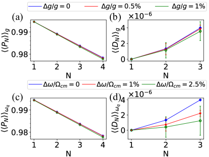
Figure 9: Impact of inhomogeneities in qubit-cavity couplings $\delta g_{j}$ and qubit frequencies $\delta\omega_{j}$ on the performance of the synchronized multiphoton emitter. (a) Average $N$-photon generation probabilities $\langle\!\langle P_{N}\rangle\!\rangle_{g}$ up to $N=4$ for coupling disorder strengths $\Delta g/g=0$ (blue), $\Delta g/g=0.5\%$ (red), and $\Delta g/g=1\%$ (green). (b) Average demultiplexing error $\langle\!\langle D_{N}\rangle\!\rangle_{g}$ up to $N=3$, for the same disorder values as in (a). (c)-(d) Analogous calculations as in (a)-(b), but considering $\langle\!\langle P_{N}\rangle\!\rangle_{\omega_{q}}$ and $\langle\!\langle D_{N}\rangle\!\rangle_{\omega_{q}}$ with disorder in the qubit frequencies $\delta\omega^{j}_{q}$. We consider disorder strengths $\Delta\omega_{q}/\Omega_{\rm cm}=0$ (blue), $\Delta\omega_{q}/\Omega_{\rm cm}=1\%$ (red), and $\Delta\omega_{q}/\Omega_{\rm cm}=2.5\%$ (green). All calculations are performed using the parameter set B of Table 1 and up to $M=3\cdot 10^{5}$ realizations of each type of disorder.

Finally, we analyze the impact of inhomogeneous qubit frequencies $\omega_{q}^{j}=\omega_{q}+\delta\omega^{j}_{q}$, which lead to slightly different qubit detunings with respect to the cavity driving frequency $\omega_{d}$, i.e. $\delta_{j}=\delta-\delta\omega_{q}^{j}$, where $\delta=\omega_{d}-\omega_{q}$ is the average detuning. We can set $\omega_{d}$ to compensate for the cavity-induced Lamb-shift $\delta=\delta_{\rm cm}$, but the remaining inhomogeneities will lead to slightly different probabilities of preparing the $|e\rangle_{j}$ states on each qubit, i.e.

$$P_{e}^{j}\approx 1-\frac{1}{4}\left(\frac{\delta\omega^{j}_{q}}{\Omega_{\rm cm}}\right)^{2}+{\cal O}{\color[rgb]{0,0,0}\left(\frac{\delta\omega^{j}_{q}}{\Omega_{\rm cm}}\right)^{4}.}$$ (36)

Therefore, frequency inhomogeneties should also be controlled $\delta\omega_{q}^{j}\ll\Omega_{\rm cm}$, in order to have a high quality synchronization and demultiplexing. We discussed in Sec. III.1 that the qubit frequencies can be fine-tuned by sending specific DC currents on each antenna channel. With this we can make all qubits nearly resonant up to a tuning imprecision in the range $\Delta\omega_{q}/2\pi\lesssim 1$MHz DiCarlo et al. (2009); Barends et al. (2013); Pechal et al. (2014); Arrangoiz-Arriola et al. (2019). This means that a frequency disorder of order $\Delta\omega_{q}/\Omega_{\rm cm}\lesssim 2.5\%$ is achievable with state-of-the-art technology. In Figs. 9(c)-(d), we calculate $\langle\!\langle P_{N}\rangle\!\rangle_{\omega_{q}}$ and $\langle\!\langle D_{N}\rangle\!\rangle_{\omega_{q}}$ up to $N=4$ and for frequency disorder strengths $\Delta\omega_{q}/\Omega_{\rm cm}\lesssim 0\%$ (blue), $\Delta\omega_{q}/\Omega_{\rm cm}\lesssim 1\%$ (red), and $\Delta\omega_{q}/\Omega_{\rm cm}\lesssim 2.5\%$ (green). These results confirm that under these realistic disorder conditions the $N$-photon generation efficiency $\langle\!\langle P_{N}\rangle\!\rangle_{\omega_{q}}$ is minimally altered with respect to the homogeneous prediction [cf. blue data in Fig. 9(c)]. Moreover, we observe that the demultiplexing error $\langle\!\langle D_{N}\rangle\!\rangle_{\omega_{q}}$ reduces with higher frequency disorder $\Delta\omega_{q}/\Omega_{\rm cm}$ due to the larger independence of the photon emission processes. This occurs at the expense of reducing the generation efficiency $\langle\!\langle P_{N}\rangle\!\rangle_{\omega_{q}}$ so it is not a good limit for our purpose.

The synchronized multiphoton generation scheme is thus resilient to moderate disorder in all system paremeters and we expect high $N$-photon generation efficiencies in realistic circuit-QED implementations of the device.

VI Conclusions and Outlook

In this work, we propose a scalable design for generating efficiently a large number of synchronized, independent and indistinguishable photons propagating over independent channels. The synchronization is provided by a strongly driven resonator in the bad cavity and weak-coupling limits. The resonator allows for a simultaneous and robust control of all emitters, which deposit photon into individual waveguides, at a high rate and with a high collection efficiency. Although our scheme can be implemented in cavity QED and nanophotonic platforms Welte et al. (2018); Casabone et al. (2015); Araneda et al. (2018); Reitz et al. (2013); Lodahl et al. (2015); Antón et al. (2019); Ellis et al. (2018); Goban et al. (2015), we have discussed a particularly efficient superconducting circuits implementation, with microwave resonators, superconducting qubits and microwave transmission lines Pechal et al. (2014); Zhou et al. (2020); Wang et al. (2020); Barends et al. (2013); Caldwell et al. (2018); McKay et al. (2019); Andersen et al. (2020); Dassonneville et al. (2020a).

The only intrinsic limitation for the scalability of the synchronized multiphoton device are the cavity-mediated interactions and collective decay, which can create correlations between SPSs and the emitted photons. Nevertheless, for state-of-the-art circuit QED parameters, we show that these correlations are strongly suppressed on the timescale of photon emission, and that they only induce a nearly negligible quadratic demultiplexing error $D_{N}\approx\epsilon N(N-1)$ with $\epsilon\sim 10^{-8}-10^{-6}$. Remarkably, this allows for the synchronization of up to hundreds of nearly independent single-photons, even in the presence of decoherence and disorder.

Given that, as we show, each SPS can achieve single-photon efficiency, purity, and indistinguishability above $99\%$, and the parallel operation in our device enables the efficient creation of large $N$-photon states. For instance, we predict a $30$-photon probability of $P_{30}\approx 0.72$ at a rate $C_{30}\approx 270$kHz and a $100$-photon probability of $P_{100}\approx 0.33$ at a rate $C_{100}\approx 130$kHz. This is seven orders of magnitude more efficient than the most sophisticated multiplexed SPSs up to $N=14$ Lenzini et al. (2017); Wang et al. (2017); Loredo et al. (2017); Wang et al. (2019a); Antón et al. (2019); Hummel et al. (2019). All these promising figures of merit can be further improved when implementing a more refined model for the SPSs such as three-level emitters Fischer et al. (2016), but this is independent from the efficient synchronization scheme we propose.

Scalable and deterministic sources of multi-photon states will be a key resource for realizing large-scale quantum information processing such as quantum optical neural networks Steinbrecher et al. (2019) or fault-tolerant photonic quantum computation Takeda and Furusawa (2019). In the short-term, the implemenation of our scheme can already enable quantum advantage experiments with hundreds of microwave photons such as boson sampling Brod et al. (2019) or quantum metrology Motes et al. (2015); Ge et al. (2018). Moreover, the setup and ideas introduced in this work can be further extended to scale up the generation of correlated multi-photon states Meyer-Scott et al. (2019); Pfaff et al. (2017) with engineered entanglement patterns Besse et al. (2020). Many-body methods such as Matrix-product-states Huang et al. (2019); Orús (2014) could be exploited to study the multi-photon correlations of the propagating fields, and recent multi-photon probing methods Ramos and García-Ripoll (2017); Muñoz et al. (2018); Dassonneville et al. (2020b); Lescanne et al. (2020); Le Jeannic et al. (2021) could be use to characterize them in the lab.

Appendix A Derivation of effective model for cavity synchronization

In this appendix we outline the derivation of the effective master equation (12) by performing a displacement transformation on the cavity mode [cf. Sec. A.1], and then an adiabatic elimination of the cavity fluctuations [cf. Sec. A.2].

A.1 Coherent displacement of driven cavity mode

The quantum Langevin equations Gardiner and Zoller (2004) associated to the master equation (6) read

$$\dot{a}={} -\left[\kappa/2+i\omega_{c}\right]a-i\sum_{j=1}^{N}g_{j}(\sigma_{j}^{-}+\sigma_{j}^{+})-\sqrt{\kappa}a_{\rm in}$$

$$-2i\Omega(t)\cos(\omega_{d}t),$$ (37)

$$\dot{\sigma}_{j}^{-}={} -\left[(\gamma_{j}+\gamma^{j}_{\rm loss})/2+i\omega_{j}^{q}\right]\sigma_{j}^{-}+ig_{j}(a+a)^{{\dagger}}\sigma_{j}^{z}$$

$$+\sqrt{\gamma_{j}}\sigma_{j}^{z}b_{\rm in}^{j}+\sqrt{\gamma^{j}_{\rm loss}}\sigma_{j}^{z}c_{\rm in}^{j}-i\sqrt{2\gamma_{\phi}^{j}}\chi(t)\sigma_{j}^{-},$$ (38)

$$\dot{\sigma}_{j}^{z}={} -(\gamma_{j}+\gamma^{j}_{\rm loss})(1+\sigma_{j}^{z})-2ig_{j}(a^{{\dagger}}+a)(\sigma_{j}^{+}-\sigma_{j}^{-})$$

$$-2\sqrt{\gamma_{j}}\left[\sigma_{j}^{+}b_{\rm in}^{j}+{\rm h.c.}\right]-2\sqrt{\gamma^{j}_{\rm loss}}\left[\sigma_{j}^{+}c_{\rm in}^{j}+{\rm h.c.}\right].$$ (39)

Here, $\chi(t)$ is a stochastic white noise dephasing fluctuation satisfying $\langle\!\langle\chi(t)\chi(t^{\prime})\rangle\!\rangle=\delta(t-t^{\prime})$ Ramos and García-Ripoll (2018), $a_{\rm in}(t)$ corresponds to the input noise field of the cavity mode, $b_{\rm in}^{j}(t)$ the input field of photons in antenna $j$, and $c_{\rm in}^{j}(t)$ the photonic input field of unwanted channels coupled to qubit $j$. A coherent driving on the cavity induces a coherent state component on this mode, and thus it is convenient to displace it using the transformation $a\rightarrow\alpha+\delta a$ as in Eq. (7). Here, $\delta a$ corresponds to the quantum fluctuation of the cavity mode around its classical value $\alpha$. By separating the classical and quantum cavity components, the displaced Langevin equation for the fluctuation reads

$$\delta\dot{a}={} -\left[\kappa/2+i\omega_{c}\right]\delta a-i\sum_{j=1}^{N}g_{j}(\sigma_{j}^{-}+\sigma_{j}^{+})-\sqrt{\kappa}a_{\rm in}(t),$$ (40)

and for the qubits,

$$\dot{\sigma}_{j}^{-}={} -\left[(\gamma_{j}+\gamma^{j}_{\rm loss})/2+i\omega_{j}^{q}\right]\sigma_{j}^{-}+ig_{j}(\delta a+\delta a^{{\dagger}})\sigma_{j}^{z}$$

$$+2ig_{j}{\rm Re}\{\alpha\}\sigma_{j}^{z}+\sqrt{\gamma_{j}}\sigma_{j}^{z}b_{\rm in}^{j}+\sqrt{\gamma^{j}_{\rm loss}}\sigma_{j}^{z}c_{\rm in}^{j}$$

$$-i\sqrt{2\gamma_{\phi}^{j}}\Theta(t)\sigma_{j}^{-},$$ (41)

$$\dot{\sigma}_{j}^{z}={} -(\gamma_{j}+\gamma_{\rm loss}^{j})(1+\sigma_{j}^{z})-2ig_{j}(\delta a^{{\dagger}}+\delta a)(\sigma_{j}^{+}-\sigma_{j}^{-})$$

$$-4ig_{j}{\rm Re}\{\alpha\}(\sigma_{j}^{+}-\sigma_{j}^{-})-2\sqrt{\gamma_{j}}\left[\sigma_{j}^{+}b_{\rm in}^{j}(t)+{\rm h.c.}\right]$$

$$-2\sqrt{\gamma^{j}_{\rm loss}}\left[\sigma_{j}^{+}c_{\rm in}^{j}(t)+{\rm h.c.}\right].$$ (42)

Here, $\alpha(t)$ is determined via the classical differential equation (8).

The master equation associated to the above Langevin equations (40)-(42) with the displaced cavity reads

$$\dot{\rho}^{\prime}(t)={} -i[H^{\prime}(t),\rho^{\prime}]+\kappa{\cal{D}}[\delta a]\rho^{\prime}+\sum_{j=1}^{N}\gamma_{j}{\cal{D}}[\sigma_{j}^{-}]\rho^{\prime}$$

$$+\sum_{j=1}^{N}\gamma^{j}_{\rm loss}{\cal{D}}[\sigma_{j}^{-}]\rho^{\prime}+\sum_{j=1}^{N}2\gamma_{\phi}^{j}{\cal{D}}[\sigma_{j}^{+}\sigma_{j}^{-}]\rho^{\prime},$$ (43)

where the system Hamiltonian after the displacement transformation $H^{\prime}(t)$ is given by,

$$H^{\prime}(t)={} \omega_{c}\delta a^{{\dagger}}\delta a+\sum_{j=1}^{N}\frac{\omega_{j}^{q}}{2}\sigma_{j}^{z}+\sum_{j=1}^{N}g_{j}(\delta a+\delta a^{{\dagger}})(\sigma_{j}^{-}+\sigma_{j}^{+})$$

$$+\sum_{j=1}^{N}2g_{j}{\rm Re}\{\alpha(t)\}(\sigma_{j}^{+}+\sigma_{j}^{-}).$$ (44)

Notice that the master equation (43) for the dynamics of $\delta a$ is the same as the master equation (6) for the total field $a$, except for the driving term in displaced Hamiltonian (44), which acts on the qubits rather than on the cavity as indicated in Eq. (10). This is the effective cavity-mediated driving on the qubits that allows for the synchronization of many SPSs in our scheme.

The displaced master equation (43) is very efficient to perform numerical simulations of the dynamics in the case of strong cavity driving $|\Omega(t)|\gg\kappa,|\Delta|$ because most of the cavity photons can be taken into account by the classical field $\alpha(t)$, and the fluctuation $\langle\delta a^{\dagger}\delta a\rangle$ is only weakly populated. This largely reduces the Hilbert space dimension needed to numerically simulate the dynamics of the driven cavity mode coupled to all qubits. In addition, if we consider the cavity in the weak coupling and bad cavity limit given by Eq. (11), the dynamics of the system can be further simplified by applying the rotating wave approximation (RWA) to the Hamiltonian in Eq. (44). On the one hand, since $g_{j}\ll\omega_{c}+\omega_{q}^{j}$ and the fluctuation is weakly populated, we can approximate the qubit-fluctuation coupling as

$$g_{j}(\delta a+\delta a^{{\dagger}})(\sigma_{j}^{-}+\sigma_{j}^{+})\approx g_{j}(\delta a^{\dagger}\sigma_{-}+{\rm h.c.}).$$ (45)

On the other hand, the cavity-mediated driving on the qubits can also be simplified by applying RWA as

$$2g_{j}{\rm Re}\{\alpha(t)\}(\sigma_{j}^{+}+\sigma_{j}^{-})\approx g_{j}|\alpha_{\rm ss}|f(t)(\sigma_{j}^{+}e^{-i(\omega_{d}t-\phi)}+{\rm h.c.}).$$ (46)

Here, $|\alpha_{\rm ss}|=\Omega_{0}/\sqrt{(\kappa/2)^{2}+\Delta^{2}}$ and $\phi={\rm Arctan}(2\Delta/\kappa)-\pi/2$ are the steady state amplitude and phase of the cavity displacement, respectively, and $f(t)$ is a step function profile. To demonstrate this last approximation (46), we first assume the square pulse is switched on $f(t)=1$ and the cavity is initially empty $\alpha(0)=0$. Then, the solution of the classical equation (8) for $\alpha(t)$ reads

$$\alpha(t)={} |\alpha_{\rm ss}|e^{-i(\omega_{d}t-\phi)}(1-e^{-(\kappa/2-i\Delta)t})$$

$$-\frac{\Omega_{0}}{2\omega_{d}}e^{i\omega_{d}t}(1-e^{-(\kappa/2+2i\omega_{d})t}),$$ (47)

where we have also used the inequalities $|\Delta|,\kappa\ll\omega_{d}$ valid for our parameter conditions. The first term in (47) reaches the steady state value $\sim|\alpha_{\rm ss}|e^{-i(\omega_{d}t-\phi)}$ in a timescale $\sim 1/\kappa$ and the second term causes the fast but low amplitude oscillation observed in Fig. 2(a). Even for a large driving strength $\Omega_{0}\gtrsim\omega_{d}$, the second term can be neglected with respect to the first when $|\alpha_{\rm ss}|\gg 1$ as it is the case for our parameters. Since in bad cavity limit (11) the timescale for the qubit dynamics is much longer than $\sim 1/\kappa$, we can use the steady state value $\alpha(t)\approx|\alpha_{\rm ss}|e^{-i(\omega_{d}t-\phi)}$ to approximate the cavity displacement when the drive is switched on $f(t)=1$ as it would be instantaneous for the qubits. Similarly, after the cavity reaches the steady state and it is switched off ($f(t)=0$), the dynamics in Eq. (8) predicts an exponential decay of $\alpha(t)$ with rate $\sim\kappa$. In the bad cavity limit we can also approximate this emptying of the cavity as instantaneous for the qubit and thus $\alpha(t)\approx 0$ for $f(t)=0$.

In summary, under the above approximations we have $\alpha(t)\approx|\alpha_{\rm ss}|e^{-i(\omega_{d}t-\phi)}f(t)$ so that when replacing it in the last term of Eq. (44), and applying RWA provided $g_{j}|\alpha_{\rm ss}|\ll\omega_{d}$, we obtain Eq. (46). Replacing Eqs. (45)-(46) in (44), and going to a rotating frame with respect to the cavity drive frequency $\omega_{d}$, the dynamics of the system in the displaced picture is finally given by the master equation (43) with the RWA Hamiltonian:

$$H^{\prime}(t)\approx{} -\Delta\delta a^{{\dagger}}\delta a-\frac{1}{2}\sum_{j=1}^{N}\delta_{j}\sigma_{j}^{z}+\sum_{j=1}^{N}g_{j}(\delta a^{{\dagger}}\sigma_{j}^{-}+\sigma_{j}^{+}\delta a)$$

$$+\sum_{j=1}^{N}\Omega_{\rm cm}^{j}(\sigma_{j}^{+}+\sigma_{j}^{-}).$$ (48)

Here, we have defined $\Omega_{\rm cm}^{j}=g_{j}|\alpha_{\rm ss}|$ as in Eq. (14) and absorbed the constant phase $\phi$ in the definition of the qubit and fluctuation operators. The qubit detunings read $\delta_{j}=\omega_{d}-\omega_{q}^{j}$ as in the main text.

A.2 Adiabatic elimination of cavity fluctuations

As discussed in the previous subsection, in the bad cavity limit $g_{j},|\delta_{j}|\ll\kappa$, the cavity reaches very quickly a coherent steady state, with its quantum fluctuations $\delta a$ close to the vacuum state $|0\rangle$. In this situation it is convenient to adiabatically eliminate the cavity fluctuation and obtain an effective dynamics for the degrees of freedom of the qubits only. To do so, we formally integrate Eq. (40) and apply Markov approximation provided the qubits’ dynamics evolves slowly on the time-scale $\sim 1/\kappa$. As a result, we get

$$\delta a(t)\approx{} -i\sum_{j}\frac{g_{j}}{(\kappa/2-i\Delta)}\sigma_{j}^{-}(t)-\frac{\sqrt{\kappa}}{(\kappa/2-i\Delta)}a_{\rm in}(t)$$

$${\color[rgb]{0,0,0}-i\sum_{j}\frac{g_{j}}{\kappa/2+i(2\omega_{d}-\Delta)}\sigma_{j}^{+}(t).}$$ (49)

Replacing the above expressions in the original quantum Langevin equations (38)-(39), applying RWA, and going to a rotating frame with frequency $\omega_{d}$, we obtain the effective dynamics of the qubits, given by the Langevin equations

$$\dot{\sigma}_{j}^{-}={} -\left[(\gamma_{j}+\gamma^{j}_{\rm loss}+\gamma_{\rm cm}^{j})/2-i(\delta_{j}-\delta^{j}_{\rm cm})\right]\sigma_{j}^{-}$$ (50)

$$+i\Omega_{\rm cm}^{j}f(t)\sigma_{j}^{z}+\sum_{l\neq j}\frac{g_{j}g_{l}}{(\kappa/2-i\Delta)}\sigma_{j}^{z}\sigma_{j}^{-}+\sqrt{\gamma^{j}_{\rm cm}}\sigma_{j}^{z}a_{\rm in}$$

$$+\sqrt{\gamma_{j}}\sigma_{j}^{z}b_{\rm in}^{j}+\sqrt{\gamma^{j}_{\rm loss}}\sigma_{j}^{z}c_{\rm in}^{j}-i\sqrt{2\gamma_{\phi}^{j}}\Theta(t)\sigma_{j}^{-},$$

$$\dot{\sigma}_{j}^{z}={} -(\gamma_{j}+\gamma_{\rm loss}^{j}+\gamma_{\rm cm}^{j})(1+\sigma_{j}^{z})-2i\Omega_{\rm cm}^{j}f(t)(\sigma_{j}^{+}-\sigma_{j}^{-})$$

$$-2\sum_{l\neq j}\left[\frac{g_{j}g_{l}}{(\kappa/2-i\Delta)}\sigma_{j}^{+}\sigma_{l}^{-}+{\rm h.c.}\right]$$

$$-2\sqrt{\gamma^{j}_{\rm cm}}\left[\sigma_{j}^{+}a_{\rm in}+{\rm h.c.}\right]-2\sqrt{\gamma_{j}}\left[\sigma_{j}^{+}b_{\rm in}^{j}+{\rm h.c.}\right]$$

$$-2\sqrt{\gamma^{j}_{\rm loss}}\left[\sigma_{j}^{+}c_{\rm in}^{j}+{\rm h.c.}\right].$$ (51)

Here, the effective cavity-mediated decay $\gamma_{\rm cm}^{j}$, detuning $\delta_{\rm cm}^{j}$, hopping $J_{\rm cm}^{jl}$, and driving strength $\Omega_{\rm cm}^{j}$ are defined in Eqs. (14)-(17).

Finally, we can find a master equation which leads to the same effective Langenvin equations in Eqs. (50)-(51). This effective master equation, which incorporates the adiabatic elimination of the cavity mode, is given in Eqs. (12)-(13).

Appendix B Photon counting and calculation of photon generation probabilities

Photon detection and counting lies at the heart of Quantum Optics and thus plenty of methods have been developed over time Gardiner and Zoller (2004); Plenio and Knight (1998). In this Appendix we describe two methods for quantifying the efficiencies and photon statistics from the output of many SPSs. In Sec. B.1 we introduce an original photon counting method that we developed based on extending the master equation formalism. Then, in Sec. B.2, we discuss a more standard photon counting method using the quantum trajectory (QT) approach. This is useful when the Hilbert space of the system becomes very large, but at the expense of losing precision in the computation of the averages.

B.1 Photon counting in master equation formalism

In the master equation dynamics the information about the emission of photons into the bath is omitted, and therefore one typically resorts to the input-output formalism (cf. Sec. C and Ref. Gardiner and Zoller (2004)) in order to relate measurable photonic quantities to multi-time system correlations. Nevertheless, obtaining the photon statistics from these system correlations involves the computation of multi-dimensional integrals over time, which can be very computationally costly and inefficient when scaling up the number of emitters or photons to probe.

To tackle the above problem, we developed a non-conventional photon counting method that extends the master equation formalism by reincorporating the information of the emitted photons. To do so, we simulate photon counters at each output channel $j=1,\dots,N$ of the system as quantum “boxes” that dynamically count the number of quantum jumps performed by each emitter and thereby the emitted photons. An adequate modeling of the photon counters is crucial to ensure that their presence does not alter the physical dynamics of the system and this is what we detail in the following. First, our method requires extending the Hilbert space of the system ${\cal H}_{\rm sys}$ as

$${\cal H}_{\rm ext}={\cal H}_{\rm sys}\otimes{\cal H}^{\rm c}_{1}\otimes\dots\otimes{\cal H}^{\rm c}_{N},$$ (52)

where ${\cal H}_{j}^{\rm c}={\rm span}\{\ket{0}_{j},\ket{1}_{j},\dots,\ket{N_{c}}_{j}\}$ correspond to the extra Hilbert spaces of each photon counter $j=1,\dots,N$ spanned by Fock states $|n\rangle_{j}$ that count the detected photons from $n=0$ to a maximum value $n=N_{c}$. The dimension of the extended Hilbert space grows exponentially as

$${\rm dim}\{{\cal H}_{\rm ext}\}={\rm dim}\{{\cal H}_{\rm sys}\}(1+N_{c})^{N},$$ (53)

but as long as the total dimension fits in ${\rm dim}\{{\cal H}_{\rm ext}\}\lesssim 2^{10}$ our method provides a fast and efficient way to numerically calculate the few-photon statistics of multiple emitters within a purely master equation approach. For any Markovian master equation for a system state $\tilde{\rho}(t)$, one can find an extended master equation that incorporates the few-photon counting statistics in the dynamics. The general recipe is actually very simple and thus we explain it directly on the synchronized multiphoton device described by Eq. (12). In this case, the extended master equation reads

$$\dot{\rho}_{\rm ext}={} -i[\tilde{H}(t),\rho_{\rm ext}]+\sum_{j=1}^{N}\gamma_{j}{\cal{D}}[\sigma_{j}^{-}S_{j}^{\dagger}]\rho_{\rm ext}$$

$${}+ \sum_{j=1}^{N}\gamma^{j}_{\rm loss}{\cal{D}}[\sigma_{j}^{-}]\rho_{\rm ext}+\sum_{j=1}^{N}2\gamma_{\phi}^{j}{\cal{D}}[\sigma_{j}^{+}\sigma_{j}^{-}]\rho_{\rm ext}$$

$$+{\cal{D}}\left[\sum_{j=1}^{N}\sqrt{\gamma^{j}_{\rm cm}}\sigma_{j}^{-}\right]\rho_{\rm ext},$$ (54)

where $\rho_{\rm ext}$ is the density operator of the extended system including counters. Importantly, the extended master equation looks identical to the original in Eq. (12), except for the inclusion of the counting operators $S_{j}^{\dagger}$ in the Lindblad terms $\sim\gamma_{j}{\cal{D}}[\sigma_{j}^{-}S_{j}^{\dagger}]$ associated to the photon emissions we want to characterize. The counting operator is a cyclic and unitary operator defined as

$$S_{j}^{\dagger}=\sum_{n=0}^{N_{c}-1}|n+1\rangle_{j}\langle n|+|0\rangle_{j}\langle N_{c}|,$$ (55)

and therefore every time the emitter $j$ performs a quantum jump and decays into its antenna with rate $\gamma_{j}$, $S_{j}^{\dagger}$ adds a new photon to the counter box $j$ as

$$S_{j}^{\dagger}|n\rangle_{j}={} |n+1\rangle_{j},\quad n\neq N_{c}.$$ (56)

When a counter reaches its maximum state $|N_{c}\rangle_{j}$, additional quantum jumps would reset the counter as,

$$S_{j}^{\dagger}|N_{c}\rangle_{j}={} |0\rangle_{j},$$ (57)

and therefore it is very important to choose $N_{c}$ large enough to avoid reaching this limit and properly account for the physically emitted photons. Using the cyclic definition of $S_{j}^{\dagger}$ in Eq. (55), as well as their unitarity properties $S_{j}^{\dagger}S_{j}=S_{j}S_{j}^{\dagger}=1$, we can take partial trace on the extended master equation (54) and show that we exactly recover the system dynamics as

$$\tilde{\rho}(t)={\rm Tr}_{\rm c}\{\rho_{\rm ext}(t)\},$$ (58)

where $\tilde{\rho}(t)$ is the state of the system governed by the original master equation without photon counting (12).

In practical calculations we therefore solve for the extended state $\rho_{\rm ext}(t)$ in Eq. (54), and we then obtain the few-photon statistics of the emitted photons by taking simple expectation values on $\rho_{\rm ext}(t)$. In particular, the probability ${\cal P}_{n}^{j}$ to count $n$ photons in channel $j$ is calculated as

$${\cal P}_{n}^{j}(t)={\rm Tr}\{\Lambda_{n}^{j}\rho_{\rm ext}(t)\},$$ (59)

where the projection operators $\Lambda_{n}^{j}$ on the counter Fock states $|n\rangle_{j}$ are defined as

$$\Lambda_{n}^{j}=|n\rangle_{j}\langle n|.$$ (60)

More generally, the probability to detect $n_{1},\dots,n_{N}$ photons in output channels $j=1,\dots,N$, respectively, is obtained by products of the projectors as

$$\Pi_{n_{1}\dots n_{N}}^{1\dots N}={\rm Tr}\{\Lambda_{n_{1}}^{1}\dots\Lambda_{n_{N}}^{N}\rho_{\rm ext}\}.$$ (61)

Using equation (61) we can calculate the full few-photon statistics of the system as long as the evolution of the extended master equation (54) is numerically tractable. This method is particularly suited for characterizing the efficiency of SPSs since in that case we expect the photon statistics to be strongly peaked at $n_{j}\approx 1$ and therefore taking $N_{c}=1$ or $N_{c}=2$ on each counter may be enough. In most calculations shown in the main text, we take $N_{c}=1$ and quantify the probability of emitting one photon on each of the $N$ channels simultaneously by computing

$$P_{N}=\Pi_{1\dots 1}^{1\dots N}={\rm Tr}\{\Lambda_{1}^{1}\dots\Lambda_{1}^{N}\rho_{\rm ext}\}.$$ (62)

In the general case, however, it is important to ensure that the occupation of the last state of the counters is negligible, so that the photon statistics is not affected by the finite size of the counters.

B.2 Photon counting in quantum trajectories formalism

The most natural way to implement an ideal photon counting is within the formalism of quantum trajectories (QT) and continuous measurements Plenio and Knight (1998); Daley (2014); Dalibard et al. (1992); Mølmer et al. (1993); Dum et al. (1992). Here, the physics of quantum jumps is explicitly simulated during the open system evolution and therefore it is very natural to count them and thereby infer the photon statistics.

The QT interpretation requires re-expressing the master equation (12) of our SPS synchronization and demultiplexing system as Plenio and Knight (1998); Daley (2014)

$$\dot{\tilde{\rho}}(t)=-i(H_{\rm nh}\tilde{\rho}-\tilde{\rho}H_{\rm nh}^{\dagger})+\sum_{q=1}^{Q}c_{q}\tilde{\rho}c_{q}^{\dagger}.$$ (63)

Here, $H_{\rm nh}$ is the non-Hermitian Hamiltonian of the system given by

$$H_{\rm nh}=\tilde{H}-\frac{i}{2}\sum_{q=1}^{Q}c_{q}^{\dagger}c_{q},$$ (64)

with $\tilde{H}$ the standard system Hamiltonian in Eq. (13) and $c_{q}$ denoting the $Q=3N+1$ jump operators appearing in the master equation (12). Using the index $j=1,\dots,N$, which describes each of the $N$ SPSs, the jump operators $c_{q}$, with $q=1,\dots,Q=3N+1$ can be decomposed as

$$c_{j}={} \sqrt{\gamma_{j}}\sigma_{j}^{-},$$ (65)

$$c_{N+j}={} \sqrt{\gamma_{\rm loss}^{j}}\sigma_{j}^{-},$$ (66)

$$c_{2N+j}={} \sqrt{2\gamma_{\phi}^{j}}\sigma_{j}^{+}\sigma_{j}^{-},$$ (67)

$$c_{3N+1}={} \sum_{j=1}^{N}\sqrt{\gamma^{j}_{\rm cm}}\sigma_{j}^{-}.$$ (68)

The dynamics of the system in the QT formalism is obtained by calculating the stochastic evolution of $m=1,\dots,M$ realizations of a pure system state $|\Psi_{m}(t)\rangle$, starting from the initial state $|\Psi_{m}(0)\rangle=\ket{g}^{\otimes N}$. The evolution of each state realization $|\Psi_{m}(t)\rangle$ combines deterministic dynamics via the non-Hermitian Schrödinger equation

$$\frac{d}{dt}\ket{\Psi_{m}(t)}=-iH_{\rm nh}\ket{\Psi_{m}(t)},$$ (69)

and stochastic quantum jumps that project the quantum state at random times as

$$|\Psi_{m}(t)\rangle\rightarrow\frac{c_{q}|\Psi_{m}(t)\rangle}{\langle\Psi_{m}(t)|c_{q}^{\dagger}c_{q}|\Psi_{m}(t)\rangle},$$ (70)

where the specific jump operator $c_{q}$ is also randomly chosen from the $q=1,\dots,Q$ possibilities on each jump process. When solving for $M\gg 1$ realizations, one can obtain the density matrix $\tilde{\rho}(t)$ of the system from the ensemble average $\tilde{\rho}(t)=(1/M)\sum_{m=1}^{M}|\Psi_{m}(t)\rangle\langle\Psi_{m}(t)|$ or calculate the expectation value of any system operator $X$ as $\langle X(t)\rangle=(1/M)\sum_{m=1}^{M}\langle\Psi_{m}(t)|X(t)|\Psi_{m}(t)\rangle$.

Importantly, if we record the information of how many jumps of each type $c_{q}$ occurred on each of the $M$ realizations $|\Psi_{m}(t)\rangle$, we can directly access the photon statistics of the system from this data. For instance, the probability ${\cal P}_{n}^{j}$ to generate $n$ photons on antenna $j=1,\dots,N$ is calculated in the QT approach as

$${\cal P}_{n}^{j}=\frac{{\cal N}(c_{j}|n)}{M},$$ (71)

where ${\cal N}(c_{j}|n)$ denotes the number of trajectories that registered $n$ jumps with a given operator $c_{j}$ of Eq. (65). Similarly, the $N$-photon probability $P_{N}$ of generating one photon on each of the $N$ independent antennas can be statistically obtained as

$$P_{N}=\frac{{\cal N}(c_{1},c_{2},\dots,c_{N}|1,1,\dots,1)}{M},$$ (72)

where ${\cal N}(c_{1},c_{2},\dots,c_{N}|1,1,\dots,1)$ denotes the number of trajectories that registered exactly one jump of each $c_{j}$ operator in Eq. (65), for $j=1,\dots,N$.

When calculating many trajectories $M\gg 1$ of the system dynamics, we can gather enough quantum jump data and determine the photon emission probabilities (71) and (72) with low statistical error. Since this error decreases as $\sim M^{-1/2}$, we typically require on the order of $M\sim 10^{3}-10^{4}$ trajectories to obtain meaningful results with an error on order $\sim 10^{-2}-10^{-3}$. In practice, this makes the calculation of ${\cal P}^{j}_{n}$ and $P_{N}$ less precise than the extended master equation method in Sec. B.1. Nevertheless, the advantage of QT formalism is that we evolve pure states instead of density matrices and that it avoids extending the Hilbert space dimension to include counters as in the extended master equation method. This two key aspects allows us to dramatically reduce the Hilbert space for the simulations and thus to treat much larger systems composed of many more SPSs [cf. the scalability calculations in Fig. 6].

Appendix C Photon correlations and input-output formalism

In Secs. III.4-III.5, we discuss how to quantify multi-photon contamination and photon indistinguishability in the emission of SPSs via second-order photon correlation functions. These photon correlations are measured via coincidence counts either in the Hanbury Brown and Twiss (HBT) or the Hong-Ou-Mandel (HOM) configurations, and can be expressed as

$$G_{\rm HBT}^{(2),j}(\tau)={} \int_{0}^{\infty}\!\!\!\!dt\langle b^{j{\dagger}}_{\rm out}(t)b^{j{\dagger}}_{\rm out}(t+\tau)b^{j}_{\rm out}(t+\tau)b^{j}_{\rm out}(t)\rangle,$$ (73)

$$G_{\rm HOM}^{(2),jl}(\tau)\!={} \!\!\!\int_{0}^{\infty}\!\!\!\!\!\!dt\langle b_{BS}^{1(jl){\dagger}}\!(t)b_{BS}^{2(jl){\dagger}}\!(t\!+\!\tau)b_{BS}^{2(jl)}(t\!+\!\tau)b_{BS}^{1(jl)}\!(t)\rangle.$$ (74)

In the HBT correlations (73), the operators $b^{j}_{\rm out}(t)$ annihilates an output photon on the antenna channel $j$ at time $t$, and in HOM correlations (74), $b_{BS}^{1(jl)}(t)=[b^{j}_{\rm out}(t)+b^{l}_{\rm out}(t)]/\sqrt{2}$, and $b_{BS}^{2(jl)}(t)=[b^{j}_{\rm out}(t)-b^{l}_{\rm out}(t)]/\sqrt{2}$ correspond to the photonic output operators after passing through a beamsplitter that connects antennas two antennas $j$ and $k$.

As explained in Secs. III.4-III.5, it is convenient to define normalized second-order correlation functions at zero time delay, which in the case of pulsed emission read,

$$g_{\rm HBT}^{(2),j}[0]{} =\frac{\int_{0}^{\frac{1}{2R}}d\tau G_{\rm HBT}^{(2),j}(\tau)}{\left(\int_{0}^{\frac{1}{2R}}dt\langle b_{\rm out}^{j{\dagger}}(t)b_{\rm out}^{j}(t)\rangle\right)^{2}},$$ (75)

$$g_{\rm HOM}^{(2),jl}[0]{} =\frac{\int_{0}^{\frac{1}{2R}}d\tau G_{\rm HOM}^{(2),jl}(\tau)}{\prod_{k=1}^{2}\left(\int_{0}^{\frac{1}{2R}}dt\langle b_{BS}^{k(jl){\dagger}}(t)b_{BS}^{k(jl)}(t)\rangle\right)}.$$ (76)

To express the photon correlations in Eqs. (73)-(76) in terms of two-time system correlations, we can use the input-output relation, which read

$$b^{j}_{\rm out}(t)=b^{j}_{\rm in}(t)+\sqrt{\gamma_{j}}\sigma_{j}^{-}(t),$$ (77)

where $\sigma_{j}^{-}(t)$ is the Pauli operator of qubit $j=1,\dots,N$. In addition, the input field $b^{j}_{\rm in}(t)$ is the same operator that appears in the quantum Langevin equations (42) or (51), and it can be expressed as a Fourier transform over the annihilation operators $b_{j}(\omega)$ of photons of frequency $\omega$ propagating in antenna $j$, namely

$$b_{\rm in}^{j}(t)={} \frac{1}{\sqrt{2\pi}}\int_{-\infty}^{\infty}d\omega e^{-i\omega t}b_{j}(\omega).$$ (78)

If we use the input-output relation (77) into the correlations functions in Eqs. (75)-(76), and consider that all antennas are initially in vacuum state $|0\rangle$, we obtain

$$g_{\rm HBT}^{(2),j}[0]{} =\frac{\int_{0}^{\frac{1}{2R}}\!d\tau\!\int_{0}^{\infty}\!dt\langle\sigma^{+}_{j}(t)\sigma^{+}_{j}(t+\tau)\sigma^{-}_{j}(t+\tau)\sigma^{-}_{j}(t)\rangle}{\left(\int_{0}^{\frac{1}{2R}}dt\langle\sigma_{j}^{+}(t)\sigma_{j}^{-}(t)\rangle\right)^{2}},$$ (79)

and

$$g_{\rm HOM}^{(2),jl}[0]{} =\frac{\int_{0}^{\frac{1}{2R}}\!d\tau\!\!\int_{0}^{\infty}\!\!dt\langle\xi_{1}^{(jl){\dagger}}\!(t)\xi_{2}^{(jl){\dagger}}\!(t\!+\!\tau)\xi_{2}^{(jl)}\!(t\!+\!\tau)\xi^{(jl)}_{1}\!(t)\rangle}{\prod_{k=1}^{2}\left(\int_{0}^{\frac{1}{2R}}dt\langle\xi_{k}^{(jl){\dagger}}(t)\xi_{k}^{(jl)}\!(t)\rangle\right)}.$$ (80)

Here, the superposition system operators between qubits $j$ and $l$ read

$$\xi_{1}^{(jl)}(t)=(\sqrt{\gamma_{j}}\sigma_{j}^{-}(t)+\sqrt{\gamma_{l}}\sigma_{l}^{-}(t))/\sqrt{2},$$ (81)

$$\xi_{2}^{(jl)}(t)=(\sqrt{\gamma_{j}}\sigma_{j}^{-}(t)-\sqrt{\gamma_{l}}\sigma_{l}^{-}(t))/\sqrt{2}.$$ (82)

Finally, we can use the Eq. (12) together with the quantum fluctuation regression theorem Gardiner and Zoller (2004) to calculate the system expectation values $\langle\sigma_{j}^{+}(t)\sigma_{j}^{-}(t)\rangle$ and $\langle\xi_{k}^{(jl){\dagger}}(t)\xi_{k}^{(jl)}\!(t)\rangle$, as well as the two-time system correlation functions $\langle\sigma^{+}_{j}(t)\sigma^{+}_{j}(t+\tau)\sigma^{-}_{j}(t+\tau)\sigma^{-}_{j}(t)\rangle$ and $\langle\xi_{1}^{(jl){\dagger}}\!(t)\xi_{2}^{(jl){\dagger}}\!(t\!+\!\tau)\xi_{2}^{(jl)}\!(t\!+\!\tau)\xi^{(jl)}_{1}\!(t)\rangle$. After calculating these quantities, we replace them into Eqs. (79)-(80), and perform the corresponding integrals over time $t$ and time delay $\tau$ to obtain the results for the HBT and HOM second-order correlations functions shown in Secs. III.4-III.5.

References

- Eisaman et al. (2011) M. D. Eisaman, J. Fan, A. Migdall, and S. V. Polyakov, Review of Scientific Instruments 82, 071101 (2011).
- Senellart et al. (2017) P. Senellart, G. Solomon, and A. White, Nature Nanotech 12, 1026 (2017).
- Slussarenko and Pryde (2019) S. Slussarenko and G. J. Pryde, Applied Physics Reviews 6, 041303 (2019).
- Knill et al. (2001) E. Knill, R. Laflamme, and G. J. Milburn, Nature 409, 46 (2001).
- Kok et al. (2007) P. Kok, W. J. Munro, K. Nemoto, T. C. Ralph, J. P. Dowling, and G. J. Milburn, Rev. Mod. Phys. 79, 135 (2007).
- Tiecke et al. (2014) T. G. Tiecke, J. D. Thompson, N. P. de Leon, L. R. Liu, V. Vuletic, and M. D. Lukin, Nature 508, 241 (2014).
- Tiarks et al. (2016) D. Tiarks, S. Schmidt, G. Rempe, and S. Duerr, Science Advances 2, e1600036 (2016).
- Takeda and Furusawa (2019) S. Takeda and A. Furusawa, APL Photonics 4, 060902 (2019), publisher: American Institute of Physics.
- Lodahl (2017) P. Lodahl, arXiv:1707.02094 [quant-ph] (2017), arXiv: 1707.02094.
- Aspuru-Guzik and Walther (2012) A. Aspuru-Guzik and P. Walther, Nature Physics 8, 285 (2012).
- Hartmann (2016) M. J. Hartmann, J. Opt. 18, 104005 (2016).
- Briegel et al. (1998) H.-J. Briegel, W. Duer, J. I. Cirac, and P. Zoller, Phys. Rev. Lett. 81, 5932 (1998).
- Sangouard et al. (2011) N. Sangouard, C. Simon, H. de Riedmatten, and N. Gisin, Rev. Mod. Phys. 83, 33 (2011).
- Llewellyn et al. (2019) D. Llewellyn, Y. Ding, I. I. Faruque, S. Paesani, D. Bacco, R. Santagati, Y.-J. Qian, Y. Li, Y.-F. Xiao, M. Huber, M. Malik, G. F. Sinclair, X. Zhou, K. Rottwitt, J. L. O’Brien, J. G. Rarity, Q. Gong, L. K. Oxenlowe, J. Wang, and M. G. Thompson, Nat. Phys. , 1 (2019).
- Gisin et al. (2002) N. Gisin, G. Ribordy, W. Tittel, and H. Zbinden, Rev. Mod. Phys. 74, 145 (2002).
- Motes et al. (2015) K. R. Motes, J. P. Olson, E. J. Rabeaux, J. P. Dowling, S. J. Olson, and P. P. Rohde, Phys. Rev. Lett. 114, 170802 (2015), publisher: American Physical Society.
- Ge et al. (2018) W. Ge, K. Jacobs, Z. Eldredge, A. V. Gorshkov, and M. Foss-Feig, Phys. Rev. Lett. 121, 043604 (2018), publisher: American Physical Society.
- Brod et al. (2019) D. J. Brod, E. F. Galvão, A. Crespi, R. Osellame, N. Spagnolo, and F. Sciarrino, AP 1, 034001 (2019), publisher: International Society for Optics and Photonics.
- Wang et al. (2017) H. Wang, Y. He, Y.-H. Li, Z.-E. Su, B. Li, H.-L. Huang, X. Ding, M.-C. Chen, C. Liu, J. Qin, J.-P. Li, Y.-M. He, C. Schneider, M. Kamp, C.-Z. Peng, S. Höfling, C.-Y. Lu, and J.-W. Pan, Nature Photonics 11, 361 (2017).
- Loredo et al. (2017) J. C. Loredo, M. A. Broome, P. Hilaire, O. Gazzano, I. Sagnes, A. Lemaitre, M. P. Almeida, P. Senellart, and A. G. White, Phys. Rev. Lett. 118, 130503 (2017).
- Wang et al. (2019a) H. Wang, J. Qin, X. Ding, M.-C. Chen, S. Chen, X. You, Y.-M. He, X. Jiang, L. You, Z. Wang, C. Schneider, J. J. Renema, S. Höfling, C.-Y. Lu, and J.-W. Pan, Phys. Rev. Lett. 123, 250503 (2019a).
- Steinbrecher et al. (2019) G. R. Steinbrecher, J. P. Olson, D. Englund, and J. Carolan, npj Quantum Information 5, 1 (2019), number: 1 Publisher: Nature Publishing Group.
- Fischer et al. (2016) K. A. Fischer, K. Müller, K. G. Lagoudakis, and J. Vučković, New J. Phys. 18, 113053 (2016).
- He and Barkai (2006) Y. He and E. Barkai, Phys. Chem. Chem. Phys. 8, 5056 (2006).
- He (2006) Y. He, Phys. Rev. A 74 (2006), 10.1103/PhysRevA.74.011803.
- McKeever et al. (2004) J. McKeever, A. Boca, A. D. Boozer, R. Miller, J. R. Buck, A. Kuzmich, and H. J. Kimble, Science 303, 1992 (2004), publisher: American Association for the Advancement of Science Section: Report.
- Hijlkema et al. (2007) M. Hijlkema, B. Weber, H. P. Specht, S. C. Webster, A. Kuhn, and G. Rempe, Nature Physics 3, 253 (2007), number: 4 Publisher: Nature Publishing Group.
- Brunel et al. (1999) C. Brunel, B. Lounis, P. Tamarat, and M. Orrit, Phys. Rev. Lett. 83, 2722 (1999), publisher: American Physical Society.
- Ahtee et al. (2009) V. Ahtee, R. Lettow, R. Pfab, A. Renn, E. Ikonen, S. Götzinger, and V. Sandoghdar, Journal of Modern Optics 56, 161 (2009), publisher: Taylor & Francis _eprint: https://doi.org/10.1080/09500340802464657.
- Rezai et al. (2018) M. Rezai, J. Wrachtrup, and I. Gerhardt, Phys. Rev. X 8, 031026 (2018).
- Almendros et al. (2009) M. Almendros, J. Huwer, N. Piro, F. Rohde, C. Schuck, M. Hennrich, F. Dubin, and J. Eschner, Phys. Rev. Lett. 103, 213601 (2009), publisher: American Physical Society.
- Stute et al. (2012) A. Stute, B. Casabone, P. Schindler, T. Monz, P. O. Schmidt, B. Brandstätter, T. E. Northup, and R. Blatt, Nature 485, 482 (2012), number: 7399 Publisher: Nature Publishing Group.
- Higginbottom et al. (2016) D. B. Higginbottom, L. Slodička, G. Araneda, L. Lachman, R. Filip, M. Hennrich, and R. Blatt, New J. Phys. 18, 093038 (2016).
- Sosnova et al. (2018) K. Sosnova, C. Crocker, M. Lichtman, A. Carter, S. Scarano, and C. Monroe, in Frontiers in Optics / Laser Science (2018), paper FW7A.5 (Optical Society of America, 2018) p. FW7A.5.
- Chou et al. (2004) C. W. Chou, S. V. Polyakov, A. Kuzmich, and H. J. Kimble, Phys. Rev. Lett. 92, 213601 (2004), publisher: American Physical Society.
- Matsukevich et al. (2006) D. N. Matsukevich, T. Chanelière, S. D. Jenkins, S.-Y. Lan, T. A. B. Kennedy, and A. Kuzmich, Phys. Rev. Lett. 97, 013601 (2006), publisher: American Physical Society.
- Farrera et al. (2016) P. Farrera, G. Heinze, B. Albrecht, M. Ho, M. Chávez, C. Teo, N. Sangouard, and H. de Riedmatten, Nature Communications 7, 1 (2016), number: 1 Publisher: Nature Publishing Group.
- Ripka et al. (2018) F. Ripka, H. Kübler, R. Löw, and T. Pfau, Science 362, 446 (2018), publisher: American Association for the Advancement of Science Section: Report.
- Aharonovich et al. (2016) I. Aharonovich, D. Englund, and M. Toth, Nat Photon 10, 631 (2016).
- Santori et al. (2002) C. Santori, D. Fattal, J. Vučković, G. S. Solomon, and Y. Yamamoto, Nature 419, 594 (2002).
- Nawrath et al. (2019) C. Nawrath, F. Olbrich, M. Paul, S. L. Portalupi, M. Jetter, and P. Michler, Appl. Phys. Lett. 115, 023103 (2019), publisher: American Institute of Physics.
- Wang et al. (2019b) H. Wang, H. Hu, T.-H. Chung, J. Qin, X. Yang, J.-P. Li, R.-Z. Liu, H.-S. Zhong, Y.-M. He, X. Ding, Y.-H. Deng, Q. Dai, Y.-H. Huo, S. Höfling, C.-Y. Lu, and J.-W. Pan, Phys. Rev. Lett. 122, 113602 (2019b).
- Schnauber et al. (2019) P. Schnauber, A. Singh, J. Schall, S. I. Park, J. D. Song, S. Rodt, K. Srinivasan, S. Reitzenstein, and M. Davanco, Nano Lett. 19, 7164 (2019).
- Thoma et al. (2016) A. Thoma, P. Schnauber, M. Gschrey, M. Seifried, J. Wolters, J.-H. Schulze, A. Strittmatter, S. Rodt, A. Carmele, A. Knorr, T. Heindel, and S. Reitzenstein, Phys. Rev. Lett. 116, 033601 (2016).
- Dusanowski et al. (2019) Ł. Dusanowski, S.-H. Kwon, C. Schneider, and S. Höfling, Phys. Rev. Lett. 122, 173602 (2019).
- Kiršanskė et al. (2017) G. Kiršanskė, H. Thyrrestrup, R. S. Daveau, C. L. Dreeßen, T. Pregnolato, L. Midolo, P. Tighineanu, A. Javadi, S. Stobbe, R. Schott, A. Ludwig, A. D. Wieck, S. I. Park, J. D. Song, A. V. Kuhlmann, I. Söllner, M. C. Löbl, R. J. Warburton, and P. Lodahl, Phys. Rev. B 96, 165306 (2017).
- Liu et al. (2018) F. Liu, A. J. Brash, J. O’Hara, L. M. P. P. Martins, C. L. Phillips, R. J. Coles, B. Royall, E. Clarke, C. Bentham, N. Prtljaga, I. E. Itskevich, L. R. Wilson, M. S. Skolnick, and A. M. Fox, Nature Nanotech 13, 835 (2018).
- Uppu et al. (2020) R. Uppu, F. T. Pedersen, Y. Wang, C. T. Olesen, C. Papon, X. Zhou, L. Midolo, S. Scholz, A. D. Wieck, A. Ludwig, and P. Lodahl, arXiv:2003.08919 [physics, physics:quant-ph] (2020), arXiv: 2003.08919.
- Rodiek et al. (2017) B. Rodiek, M. Lopez, H. Hofer, G. Porrovecchio, M. Smid, X.-L. Chu, S. Gotzinger, V. Sandoghdar, S. Lindner, C. Becher, and S. Kuck, Optica, OPTICA 4, 71 (2017).
- Sipahigil et al. (2014) A. Sipahigil, K. D. Jahnke, L. J. Rogers, T. Teraji, J. Isoya, A. S. Zibrov, F. Jelezko, and M. D. Lukin, Phys. Rev. Lett. 113, 113602 (2014).
- Alléaume et al. (2004) R. Alléaume, F. Treussart, G. Messin, Y. Dumeige, J.-F. Roch, A. Beveratos, R. Brouri-Tualle, J.-P. Poizat, and P. Grangier, New J. Phys. 6, 92 (2004), publisher: IOP Publishing.
- Gaebel et al. (2004) T. Gaebel, I. Popa, A. Gruber, M. Domhan, F. Jelezko, and J. Wrachtrup, New J. Phys. 6, 98 (2004), publisher: IOP Publishing.
- Wu et al. (2007) E. Wu, J. R. Rabeau, G. Roger, F. Treussart, H. Zeng, P. Grangier, S. Prawer, and J.-F. Roch, New J. Phys. 9, 434 (2007), publisher: IOP Publishing.
- Babinec et al. (2010) T. M. Babinec, B. J. M. Hausmann, M. Khan, Y. Zhang, J. R. Maze, P. R. Hemmer, and M. Lončar, Nature Nanotechnology 5, 195 (2010), number: 3 Publisher: Nature Publishing Group.
- Tchernij et al. (2017) S. D. Tchernij, T. Herzig, J. Forneris, J. Küpper, S. Pezzagna, P. Traina, E. Moreva, I. P. Degiovanni, G. Brida, N. Skukan, M. Genovese, M. Jakšić, J. Meijer, and P. Olivero, ACS Photonics 4, 2580 (2017), publisher: American Chemical Society.
- Neu et al. (2011) E. Neu, D. Steinmetz, J. Riedrich-Möller, S. Gsell, M. Fischer, M. Schreck, and C. Becher, New J. Phys. 13, 025012 (2011), publisher: IOP Publishing.
- Schröder et al. (2011) T. Schröder, F. Gädeke, M. J. Banholzer, and O. Benson, New J. Phys. 13, 055017 (2011), publisher: IOP Publishing.
- Wang et al. (2019c) H. Wang, Y.-M. He, T.-H. Chung, H. Hu, Y. Yu, S. Chen, X. Ding, M.-C. Chen, J. Qin, X. Yang, R.-Z. Liu, Z.-C. Duan, J.-P. Li, S. Gerhardt, K. Winkler, J. Jurkat, L.-J. Wang, N. Gregersen, Y.-H. Huo, Q. Dai, S. Yu, S. Höfling, C.-Y. Lu, and J.-W. Pan, Nat. Photonics 13, 770 (2019c).
- Houck et al. (2007) A. A. Houck, D. I. Schuster, J. M. Gambetta, J. A. Schreier, B. R. Johnson, J. M. Chow, L. Frunzio, J. Majer, M. H. Devoret, S. M. Girvin, and R. J. Schoelkopf, Nature 449, 328 (2007).
- Pechal et al. (2014) M. Pechal, L. Huthmacher, C. Eichler, S. Zeytinoğlu, A. A. Abdumalikov, S. Berger, A. Wallraff, and S. Filipp, Phys. Rev. X 4, 041010 (2014).
- Peng et al. (2016) Z. H. Peng, S. E. d. Graaf, J. S. Tsai, and O. V. Astafiev, Nature Communications 7, 12588 (2016).
- Forn-Díaz et al. (2017) P. Forn-Díaz, C. W. Warren, C. W. S. Chang, A. M. Vadiraj, and C. M. Wilson, Phys. Rev. Applied 8, 054015 (2017).
- Gasparinetti et al. (2017) S. Gasparinetti, M. Pechal, J.-C. Besse, M. Mondal, C. Eichler, and A. Wallraff, Phys. Rev. Lett. 119, 140504 (2017).
- Pfaff et al. (2017) W. Pfaff, C. J. Axline, L. D. Burkhart, U. Vool, P. Reinhold, L. Frunzio, L. Jiang, M. H. Devoret, and R. J. Schoelkopf, Nat Phys advance online publication (2017), 10.1038/nphys4143.
- Eder et al. (2018) P. Eder, T. Ramos, J. Goetz, M. Fischer, S. Pogorzalek, J. P. Martínez, E. P. Menzel, F. Loacker, E. Xie, J. J. Garcia-Ripoll, K. G. Fedorov, A. Marx, F. Deppe, and R. Gross, Supercond. Sci. Technol. 31, 115002 (2018).
- Zhou et al. (2020) Y. Zhou, Z. Peng, Y. Horiuchi, O. Astafiev, and J. Tsai, Phys. Rev. Applied 13, 034007 (2020), publisher: American Physical Society.
- Reimer and Cher (2019) M. E. Reimer and C. Cher, Nat. Photonics 13, 734 (2019).
- Patel et al. (2010) R. B. Patel, A. J. Bennett, I. Farrer, C. A. Nicoll, D. A. Ritchie, and A. J. Shields, Nature Photonics 4, 632 (2010), arXiv: 0911.3997.
- Flagg et al. (2010) E. Flagg, A. Muller, S. Polyakov, A. Ling, A. Migdall, and G. Solomon, Phys. Rev. Lett. 104, 137401 (2010).
- Moczała-Dusanowska et al. (2019) M. Moczała-Dusanowska, Ł. Dusanowski, S. Gerhardt, Y. M. He, M. Reindl, A. Rastelli, R. Trotta, N. Gregersen, S. Höfling, and C. Schneider, ACS Photonics 6, 2025 (2019).
- Ellis et al. (2018) D. J. P. Ellis, A. J. Bennett, C. Dangel, J. P. Lee, J. P. Griffiths, T. A. Mitchell, T.-K. Paraiso, P. Spencer, D. A. Ritchie, and A. J. Shields, Appl. Phys. Lett. 112, 211104 (2018), publisher: American Institute of Physics.
- Kambs and Becher (2018) B. Kambs and C. Becher, New J. Phys. 20, 115003 (2018).
- Kaneda and Kwiat (2019) F. Kaneda and P. G. Kwiat, Science Advances 5, eaaw8586 (2019).
- Hummel et al. (2019) T. Hummel, C. Ouellet-Plamondon, E. Ugur, I. Kulkova, T. Lund-Hansen, M. A. Broome, R. Uppu, and P. Lodahl, Appl. Phys. Lett. 115, 021102 (2019).
- Lenzini et al. (2017) F. Lenzini, B. Haylock, J. C. Loredo, R. A. Abrahão, N. A. Zakaria, S. Kasture, I. Sagnes, A. Lemaitre, H.-P. Phan, D. V. Dao, P. Senellart, M. P. Almeida, A. G. White, and M. Lobino, Laser & Photonics Reviews 11, 1600297 (2017).
- Pittman et al. (2002) T. B. Pittman, B. C. Jacobs, and J. D. Franson, Phys. Rev. A 66, 042303 (2002).
- Kaneda et al. (2015) F. Kaneda, B. G. Christensen, J. J. Wong, H. S. Park, K. T. McCusker, and P. G. Kwiat, Optica, OPTICA 2, 1010 (2015).
- Xiong et al. (2016) C. Xiong, X. Zhang, Z. Liu, M. J. Collins, A. Mahendra, L. G. Helt, M. J. Steel, D.-Y. Choi, C. J. Chae, P. H. W. Leong, and B. J. Eggleton, Nature Communications 7, 10853 (2016).
- Mendoza et al. (2016) G. J. Mendoza, R. Santagati, J. Munns, E. Hemsley, M. Piekarek, E. Martín-López, G. D. Marshall, D. Bonneau, M. G. Thompson, and J. L. O’Brien, Optica, OPTICA 3, 127 (2016).
- Migdall et al. (2002) A. L. Migdall, D. Branning, and S. Castelletto, Phys. Rev. A 66, 053805 (2002).
- Ma et al. (2011) X.-s. Ma, S. Zotter, J. Kofler, T. Jennewein, and A. Zeilinger, Phys. Rev. A 83, 043814 (2011), publisher: American Physical Society.
- Shapiro and Wong (2007) J. H. Shapiro and F. N. Wong, Opt. Lett., OL 32, 2698 (2007), publisher: Optical Society of America.
- Collins et al. (2013) M. Collins, C. Xiong, I. Rey, T. Vo, J. He, S. Shahnia, C. Reardon, T. Krauss, M. Steel, A. Clark, and B. Eggleton, Nat Commun 4, 2582 (2013).
- Francis-Jones et al. (2016) R. J. A. Francis-Jones, R. A. Hoggarth, and P. J. Mosley, Optica, OPTICA 3, 1270 (2016).
- Spring et al. (2017) J. B. Spring, P. L. Mennea, B. J. Metcalf, P. C. Humphreys, J. C. Gates, H. L. Rogers, C. Söller, B. J. Smith, W. S. Kolthammer, P. G. R. Smith, and I. A. Walmsley, Optica, OPTICA 4, 90 (2017).
- Grimau Puigibert et al. (2017) M. Grimau Puigibert, G. H. Aguilar, Q. Zhou, F. Marsili, M. D. Shaw, V. B. Verma, S. W. Nam, D. Oblak, and W. Tittel, Phys. Rev. Lett. 119, 083601 (2017).
- Joshi et al. (2018) C. Joshi, A. Farsi, S. Clemmen, S. Ramelow, and A. L. Gaeta, Nat Commun 9, 1 (2018).
- Hiemstra et al. (2019) T. Hiemstra, T. F. Parker, P. C. Humphreys, J. Tiedau, M. Beck, M. Karpiński, B. J. Smith, A. Eckstein, W. S. Kolthammer, and I. A. Walmsley, arXiv:1907.10355 [quant-ph] (2019), arXiv: 1907.10355.
- Christ and Silberhorn (2012) A. Christ and C. Silberhorn, Phys. Rev. A 85, 023829 (2012).
- Antón et al. (2019) C. Antón, J. C. Loredo, G. Coppola, H. Ollivier, N. Viggianiello, A. Harouri, N. Somaschi, A. Crespi, I. Sagnes, A. Lemaître, L. Lanco, R. Osellame, F. Sciarrino, and P. Senellart, arXiv:1905.00936 [cond-mat, physics:quant-ph] (2019), arXiv: 1905.00936.
- Ding et al. (2016) X. Ding, Y. He, Z.-C. Duan, N. Gregersen, M.-C. Chen, S. Unsleber, S. Maier, C. Schneider, M. Kamp, S. Höfling, C.-Y. Lu, and J.-W. Pan, Phys. Rev. Lett. 116, 020401 (2016).
- Somaschi et al. (2016) N. Somaschi, V. Giesz, L. De Santis, J. C. Loredo, M. P. Almeida, G. Hornecker, S. L. Portalupi, T. Grange, C. Antón, J. Demory, C. Gómez, I. Sagnes, N. D. Lanzillotti-Kimura, A. Lemaítre, A. Auffeves, A. G. White, L. Lanco, and P. Senellart, Nature Photonics 10, 340 (2016).
- Nunn et al. (2013) J. Nunn, N. K. Langford, W. S. Kolthammer, T. F. M. Champion, M. R. Sprague, P. S. Michelberger, X.-M. Jin, D. G. England, and I. A. Walmsley, Phys. Rev. Lett. 110, 133601 (2013).
- Bonneau et al. (2015) D. Bonneau, G. J. Mendoza, J. L. O’Brien, and M. G. Thompson, New J. Phys. 17, 043057 (2015).
- Gimeno-Segovia et al. (2017) M. Gimeno-Segovia, H. Cable, G. J. Mendoza, P. Shadbolt, J. W. Silverstone, J. Carolan, M. G. Thompson, J. L. O’Brien, and T. G. Rudolph, New Journal of Physics 19, 063013 (2017), arXiv: 1701.03306.
- Li et al. (2015) Y. Li, P. C. Humphreys, G. J. Mendoza, and S. C. Benjamin, Phys. Rev. X 5, 041007 (2015).
- DiCarlo et al. (2009) L. DiCarlo, J. M. Chow, J. M. Gambetta, L. S. Bishop, B. R. Johnson, D. I. Schuster, J. Majer, A. Blais, L. Frunzio, S. M. Girvin, and R. J. Schoelkopf, Nature 460, 240 (2009), number: 7252 Publisher: Nature Publishing Group.
- Barends et al. (2013) R. Barends, J. Kelly, A. Megrant, D. Sank, E. Jeffrey, Y. Chen, Y. Yin, B. Chiaro, J. Mutus, C. Neill, P. O’Malley, P. Roushan, J. Wenner, T. C. White, A. N. Cleland, and J. M. Martinis, Phys. Rev. Lett. 111, 080502 (2013), publisher: American Physical Society.
- Welte et al. (2018) S. Welte, B. Hacker, S. Daiss, S. Ritter, and G. Rempe, Phys. Rev. X 8, 011018 (2018).
- Casabone et al. (2015) B. Casabone, K. Friebe, B. Brandstätter, K. Schüppert, R. Blatt, and T. E. Northup, Phys. Rev. Lett. 114, 023602 (2015), publisher: American Physical Society.
- Araneda et al. (2018) G. Araneda, D. B. Higginbottom, L. Slodička, Y. Colombe, and R. Blatt, Phys. Rev. Lett. 120, 193603 (2018).
- Reitz et al. (2013) D. Reitz, C. Sayrin, R. Mitsch, P. Schneeweiss, and A. Rauschenbeutel, Phys. Rev. Lett. 110, 243603 (2013).
- Lodahl et al. (2015) P. Lodahl, S. Mahmoodian, and S. Stobbe, Rev. Mod. Phys. 87, 347 (2015).
- Mehta et al. (2020) K. K. Mehta, C. Zhang, M. Malinowski, T.-L. Nguyen, M. Stadler, and J. P. Home, arXiv:2002.02258 [physics, physics:quant-ph] (2020), arXiv: 2002.02258.
- Goban et al. (2015) A. Goban, C.-L. Hung, J. D. Hood, S.-P. Yu, J. A. Muniz, O. Painter, and H. J. Kimble, Phys. Rev. Lett. 115, 063601 (2015).
- Pietikäinen et al. (2017) I. Pietikäinen, S. Danilin, K. S. Kumar, A. Vepsäläinen, D. S. Golubev, J. Tuorila, and G. S. Paraoanu, Phys. Rev. B 96, 020501 (2017).
- Jenkins et al. (2014) M. D. Jenkins, U. Naether, M. Ciria, J. Sesé, J. Atkinson, C. Sánchez-Azqueta, E. d. Barco, J. Majer, D. Zueco, and F. Luis, Appl. Phys. Lett. 105, 162601 (2014).
- Macrì et al. (2020) V. Macrì, F. Nori, S. Savasta, and D. Zueco, Phys. Rev. A 101, 053818 (2020), publisher: American Physical Society.
- Wang et al. (2020) Z. Wang, H. Li, W. Feng, X. Song, C. Song, W. Liu, Q. Guo, X. Zhang, H. Dong, D. Zheng, H. Wang, and D.-W. Wang, Phys. Rev. Lett. 124, 013601 (2020).
- McKay et al. (2019) D. C. McKay, S. Sheldon, J. A. Smolin, J. M. Chow, and J. M. Gambetta, Phys. Rev. Lett. 122, 200502 (2019).
- Caldwell et al. (2018) S. A. Caldwell, N. Didier, C. A. Ryan, E. A. Sete, A. Hudson, P. Karalekas, R. Manenti, M. P. da Silva, R. Sinclair, E. Acala, N. Alidoust, J. Angeles, A. Bestwick, M. Block, B. Bloom, A. Bradley, C. Bui, L. Capelluto, R. Chilcott, J. Cordova, G. Crossman, M. Curtis, S. Deshpande, T. E. Bouayadi, D. Girshovich, S. Hong, K. Kuang, M. Lenihan, T. Manning, A. Marchenkov, J. Marshall, R. Maydra, Y. Mohan, W. O’Brien, C. Osborn, J. Otterbach, A. Papageorge, J.-P. Paquette, M. Pelstring, A. Polloreno, G. Prawiroatmodjo, V. Rawat, M. Reagor, R. Renzas, N. Rubin, D. Russell, M. Rust, D. Scarabelli, M. Scheer, M. Selvanayagam, R. Smith, A. Staley, M. Suska, N. Tezak, D. C. Thompson, T.-W. To, M. Vahidpour, N. Vodrahalli, T. Whyland, K. Yadav, W. Zeng, and C. Rigetti, Phys. Rev. Applied 10, 034050 (2018).
- Andersen et al. (2020) C. K. Andersen, A. Remm, S. Lazar, S. Krinner, N. Lacroix, G. J. Norris, M. Gabureac, C. Eichler, and A. Wallraff, Nature Physics , 1 (2020), publisher: Nature Publishing Group.
- Note (1) Detector inefficiencies give rise to an extra exponential factor Lenzini et al. (2017) in the -photon probability (2). See also Refs. Eisaman et al. (2011); Slussarenko and Pryde (2019) for more details.
- Kiraz et al. (2004) A. Kiraz, M. Atatüre, and A. Imamoğlu, Phys. Rev. A 69, 032305 (2004).
- Gardiner and Zoller (2004) C. Gardiner and P. Zoller, Quantum Noise (SpringerVerlag, Berlin, 3rd Ed., 2004).
- Bylander et al. (2003) J. Bylander, I. Robert-Philip, and I. Abram, Eur. Phys. J. D 22, 295 (2003).
- Arrangoiz-Arriola et al. (2019) P. Arrangoiz-Arriola, E. A. Wollack, Z. Wang, M. Pechal, W. Jiang, T. P. McKenna, J. D. Witmer, R. Van Laer, and A. H. Safavi-Naeini, Nature 571, 537 (2019), number: 7766 Publisher: Nature Publishing Group.
- Dassonneville et al. (2020a) R. Dassonneville, T. Ramos, V. Milchakov, L. Planat, É. Dumur, F. Foroughi, J. Puertas, S. Leger, K. Bharadwaj, J. Delaforce, C. Naud, W. Hasch-Guichard, J. J. García-Ripoll, N. Roch, and O. Buisson, Phys. Rev. X 10, 011045 (2020a), publisher: American Physical Society.
- Meyer-Scott et al. (2019) E. Meyer-Scott, N. Prasannan, I. Dhand, C. Eigner, V. Quiring, S. Barkhofen, B. Brecht, M. B. Plenio, and C. Silberhorn, arXiv:1908.05722 [quant-ph] (2019), arXiv: 1908.05722.
- Besse et al. (2020) J.-C. Besse, K. Reuer, M. C. Collodo, A. Wulff, L. Wernli, A. Copetudo, D. Malz, P. Magnard, A. Akin, M. Gabureac, G. J. Norris, J. I. Cirac, A. Wallraff, and C. Eichler, Nature Communications 11, 4877 (2020), number: 1 Publisher: Nature Publishing Group.
- Huang et al. (2019) H.-L. Huang, W.-S. Bao, and C. Guo, Phys. Rev. A 100, 032305 (2019), publisher: American Physical Society.
- Orús (2014) R. Orús, Annals of Physics 349, 117 (2014).
- Ramos and García-Ripoll (2017) T. Ramos and J. J. García-Ripoll, Phys. Rev. Lett. 119, 153601 (2017).
- Muñoz et al. (2018) C. S. Muñoz, F. P. Laussy, E. d. Valle, C. Tejedor, and A. González-Tudela, Optica, OPTICA 5, 14 (2018).
- Dassonneville et al. (2020b) R. Dassonneville, R. Assouly, T. Peronnin, P. Rouchon, and B. Huard, Phys. Rev. Applied 14, 044022 (2020b), publisher: American Physical Society.
- Lescanne et al. (2020) R. Lescanne, S. Deléglise, E. Albertinale, U. Réglade, T. Capelle, E. Ivanov, T. Jacqmin, Z. Leghtas, and E. Flurin, Phys. Rev. X 10, 021038 (2020), publisher: American Physical Society.
- Le Jeannic et al. (2021) H. Le Jeannic, T. Ramos, S. F. Simonsen, T. Pregnolato, Z. Liu, R. Schott, A. D. Wieck, A. Ludwig, N. Rotenberg, J. J. García-Ripoll, and P. Lodahl, Phys. Rev. Lett. 126, 023603 (2021), publisher: American Physical Society.
- Ramos and García-Ripoll (2018) T. Ramos and J. J. García-Ripoll, New J. Phys. 20, 105007 (2018).
- Plenio and Knight (1998) M. B. Plenio and P. L. Knight, Rev. Mod. Phys. 70, 101 (1998).
- Daley (2014) A. J. Daley, Advances in Physics 63, 77 (2014).
- Dalibard et al. (1992) J. Dalibard, Y. Castin, and K. Mølmer, Phys. Rev. Lett. 68, 580 (1992).
- Mølmer et al. (1993) K. Mølmer, Y. Castin, and J. Dalibard, J. Opt. Soc. Am. B 10, 524 (1993).
- Dum et al. (1992) R. Dum, P. Zoller, and H. Ritsch, Phys. Rev. A 45, 4879 (1992).