Abstract
Very massive stars occasionally expel material in colossal eruptions, driven by continuum radiation pressure rather than blast waves. Some of them rival supernovae in total radiative output, and the mass loss is crucial for subsequent evolution. Some are supernova impostors, including SN precursor outbursts, while others are true SN events shrouded by material that was ejected earlier. Luminous Blue Variable stars (LBV’s) are traditionally cited in relation with giant eruptions, though this connection is not well established. After four decades of research, the fundamental causes of giant eruptions and LBV events remain elusive. This review outlines the basic relevant physics, with a brief summary of essential observational facts. Reasons are described for the spectrum and emergent radiation temperature of an opaque outflow. Many proposed mechanisms are noted for instabilities in the star’s photosphere, in its iron opacity peak zones, and in its central region. Some of the remarks and conjectures here have not yet become familiar in the published literature.
keywords:
Eddington Limit; Eruption; Supernova Impostor; LBV; Luminous Blue Variable; Stellar Outflow; Strange Modes; Iron Opacity; Bistability Jump; Inflation0
\issuenum0
\articlenumber0
\historyReceived: 2019/12/20; Accepted: 2020/01/25; Published: 2020/02/05
\TitleRadiation-Driven Stellar Eruptions
111This is a slightly improved version of an
article in the e-book Luminous Stars in Nearby Galaxies,
https://www.mdpi.com/journal/galaxies/special_issues/Luminous
(= Galaxies 2020, 8, 10).
\AuthorKris Davidson
Contents
1. The topic and why it matters
2. History, 1965–2020
3. Categories: giant eruptions, SN impostors and precursors, LBV’s
4. Apparent temperature and spectrum of a massive outflow
5. Culpable instabilities and locales within a very massive star
6. Other issues, especially re. the most-observed example
1 Super-Eddington Events in Massive Stars
Very massive stars lose much—and possibly most—of their mass in sporadic events driven by continuum radiation. This fact has dire consequences for any attempt to predict the star’s evolution. After four decades of research, the instability mechanism has not yet been established; it may occur in the stellar core, or else in a subsurface locale, or conceivably at the base of the photosphere. Without concrete models of this process, massive-star evolution codes can generate only “proof of concept” simulations, not predictive models, because they rely on assumed mass-loss rates adjusted to give plausible results. Even worse, eruptions may illustrate the butterfly effect: the time and strength of each outburst may depend on seemingly minor details, and the total mass loss may differ greatly between two stars that appear identical at birth. And an unexpected sub-topic, involving precursors to supernova events, arose about ten years ago. Altogether, the most luminous stars cannot be understood without a greatly improved theory of radiative mass-loss events. No theorist predicted any of the main observational discoveries in this subject.
Most of the phenomena explored here are either giant eruptions (including supernova impostors, supernova precursors, and shrouded supernovae) or LBV outbursts. They have four attributes in common:
-
•
Their ratios are near or above the Eddington Limit.
-
•
Outflow speeds are usually between 100 and 800 km s-1, much slower than SN blast waves.
-
•
The eruptive photosphere temperatures range from 6000 to 20,000 K, providing enough free electrons for substantial opacity.
-
•
Observed durations are much longer than relevant dynamical timescales.
Giant eruptions are presumably driven by continuum radiation. They carry far too much kinetic energy to be “line-driven winds.” Gas pressure is quite inadequate, and blast waves are either absent or inconspicuous. MHD processes, bulk turbulent pressure, and rotational effects may play appreciable roles, but probably cannot exceed radiation pressure in these very luminous objects. Individual events have peak luminosities ranging from to more than while ejecting masses ranging from to or more. Note that continuum radiation (i.e., a super-Eddington flow) is not in itself the “cause” of an eruption. Logically the root cause must be some process or instability that either increases the local radiation flux, or enhances its ability to push a mass outflow.
This review does not include eruptions with , such as “red transients” and nova-like displays. Such events generally involve stars with or even , which are vastly more numerous than the very massive stars that produce giant eruptions (). Most likely they are highly abnormal phenomena (e.g., stellar mergers) that occur in only a tiny fraction of the stars. Giant eruptions, by contrast, tend to resemble each other regardless of their causative instabilities, and probably occur in a substantial fraction of the most massive stars – perhaps even most of them. Much of Section 4 and part of Section 5 may apply also to the lower-luminosity eruptions, however.
This article is a descriptive review like a textbook chapter, not a survey of publications. It outlines the basic physics and theoretical results with only a minimal account of the observational data. It also includes comments about some of the quoted results, with a few personal conjectures. Some of the generalities sketched here have been unfamiliar to most astronomers, even those who work on supernovae. They are conceptually simple if we refrain from exploring technicalities. One important topic—rotation— is mostly neglected here, because it would greatly lengthen the narrative and there is not yet any strong evidence that it is required for the chief processes. Binary systems are also neglected, except the special case of Car; see remarks in Section 6.
2 A Checkered History
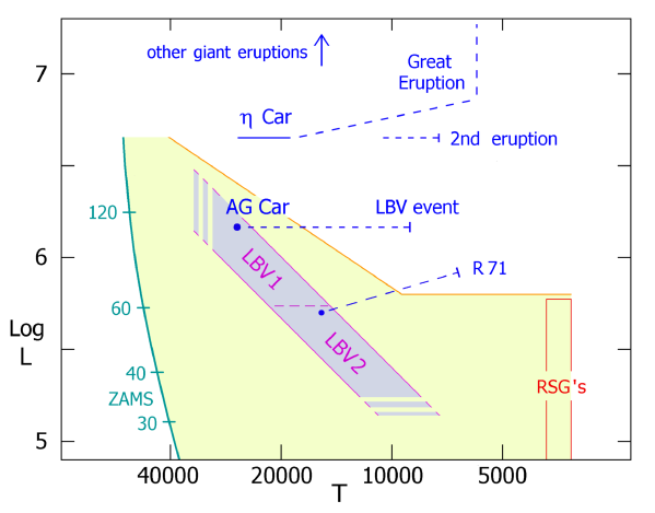
An appendix in ref. Humphreys & Davidson (1994) summarized the origins of this topic. Since only three or four giant eruptions and supernova impostors were known before 2000, they were conflated with LBV outbursts. Early discoveries followed two paths, and today we’re not yet sure whether those paths really merge. First, the examples of Car, P Cyg, SN 1961v, and SN 1954J were known before 1970 Zwicky (1965). Their outbursts produced supernova-like amounts of radiation, but with longer durations than a supernova and the stars survived.222 SN 1961v may have been a true supernova Kochanek et al. (2011); van Dyk & Matheson (2012), but, ironically, that doesn’t alter its historical role. The second path began with the recognition in 1979 of an upper boundary in the empirical HR diagram, the diagonal line in the middle of Figure 1 Humphreys & Davidson (1979). Almost no stars are found above and to the right of that line, and the rare exceptions are temporary. Since massive stars evolve almost horizontally across the diagram, this boundary indicates some sort of barrier to the outer-layer evolution of stars with . The probable explanation involves episodic mass loss as follows.
Note the various zones and boundaries in Figure 1, though in reality they are not so well defined. If a massive star loses a considerable fraction of its mass, then it cannot evolve far toward the right in the HR diagram. Thus a good way to explain the HRD boundary is to suppose that stars above 50 lose mass in some process that exceeds their line-driven winds. The S Doradus class of variable stars occurs in the “LBV1” and “LBV2” zones in Figure 1, to the left of the empirical boundary. S Dor stars are remarkably close to the Eddington Limit (Section 3.1 below), and they exhibit sporadic outbursts which can expel more material than their normal winds. If every star above 50 behaves in that way after it evolves into the LBV1 zone, then the boundary is a likely consequence. This scenario was proposed as soon as the empirical limit was recognized Humphreys & Davidson (1979). In a variant idea noted near the end of Section 3.1 below, the decisive mass loss occurs just before the stars become S Dor variables; but both hypotheses invoke eruptions in that part of the HR diagram. No better alternative has appeared in the decades since they were proposed.
Today, S Dor variables are usually called LBV’s, “Luminous Blue Variables.” Rightly or wrongly, they are frequently mentioned in connection with giant eruptions and supernova impostors. Many of them are easier to observe than eruptions in distant galaxies, and they probably offer hints to the relevant physics, Section 5 below.
Thus the key facts—episodic mass loss, and the existence of giant eruptions—were well recognized before 1995, and credible mechanisms had been noted; see many references in Humphreys & Davidson (1994). A decade later, when the mass loss rates of normal line-driven winds were revised downward Fullerton et al. (2006), the same concepts were proposed again as a way to rescue the published evolution tracks (e.g., Smith & Owocki (2006)). Unrelated to that development, extragalactic giant eruptions attracted attention after 2003 and some of them were aptly called “supernova impostors” because their stars survived Van Dyk (2005). Modern SN surveys found many examples Van Dyk & Matheson (2012), often classed among the Type IIn SNae. Some giant eruptions preceded real supernova events, the most notorious being SN 2009ip where the real SN explosion did not occur until 2012 Pastorello et al. (2013); Margutti et al. (2014). Theoretical explanations continue to be diverse and highly speculative.
3 Categories and Examples
Only a few specific objects are mentioned here, to illustrate the main phenomena.
3.1 LBV’s
The term “Luminous Blue Variable” is unfortunate in three respects: Many unrelated luminous blue stars are also variable, LBV’s are often not very blue or not strongly variable, and the term has caused extraneous objects to be included in lists of examples, often without observed outbursts Humphreys et al. (2016); Davidson et al. (2016). Thus we should regard the trigram “LBV” as an abstract label, not an acronym. Many examples are described and listed in Weis & Bomans (2020); Vink (2012); Humphreys et al. (2016). The present review includes this phenomenon because it may provide some guidance to the physics of giant eruptions, and LBV’s have been observed far more often than giant eruptions. Note, however, that suspected analogies between those two categories have not been proven and may turn out to be illusory.
LBV’s are defined by a particular form of variability like AG Car in Figure 1 Humphreys & Davidson (1994). Their hot “quiescent” states are located along a strip in the H-R Diagram (HRD) shown in the figure, sometimes called the S Doradus instability strip Wolf (1989). Its upper and lower parts, LBV1 and LBV2, represent different stages of evolution—providing a clue for theory, Section 5.1 below.
Most stars in the strip are not LBV’s. Spectroscopic analyses consistently show that genuine LBV’s have smaller masses than other stars with similar and Vink (2012); Kudritzki et al. (1989); Pauldrach & Puls (1990); Stahl, O. et al. (1990); Sterken et al. (1991); Vink & de Koter (2002). Consequently, for an LBV the Eddington parameter is close to 0.5 or somewhat larger. This is not surprising for the luminous classical LBV’s; a 60 star, for example, attains before the end of central hydrogen burning Humphreys et al. (2016). But is remarkable in zone LBV2, where most stars have . Evidently each lower-luminosity LBV has lost much of its initial mass.
Since the LBV2 stars have luminosities below the upper boundary in Figure 1, they can evolve across the HRD. Hence we can explain their low masses by supposing that they have already passed through a cool supergiant stage where mass loss was very large Humphreys & Davidson (1994). After returning to the blue side of the HRD, they now have large ratios which cause them to be LBV’s. This surmise is very strongly supported by the fact that LBV1’s are generally associated with O-type stars but LBV2’s are not Humphreys et al. (2016); Davidson et al. (2016); Aadland et al. (2018). Therefore LBV1’s are younger than LBV2’s, as expected in the evolved-LBV2 scenario. Classical LBV’s (LBV1’s) are somewhat more than 3 million years old, near or slightly after the end of core hydrogen burning. LBV2 stars are post-RSG’s near or after the end of core helium burning (Figure 1 in ref. Humphreys et al. (2016)).
The above account may seem inconsistent, because LBV’s are said to have rapid mass loss but the low masses of LBV2’s are ascribed to a different evolutionary stage. This semi-paradox arises because the two types play very different roles in this story. LBV1 outbursts probably cause enough mass loss to shape the appearance of the upper H-R Diagram. LBV2 events do not, but they are pertinent because they suggest a connection between LBV variability and the Eddington parameter as noted above. They also give a strong hint that LBV instability occurs in the outer layers, Section 5.1 below.
Figure 1 shows a well-known classical LBV, AG Carinae. It currently has and 40 to 70 , with 16000 to 25000 K at times when a major LBV event is not underway Vink (2012); Stahl et al. (2001); Groh et al. (2009, 2011). The initial mass was probably above 85 and rotation is non-negligible Groh et al. (2011). In the years 1990–1994, AG Car’s photosphere temporarily expanded by an order of magnitude with only a modest change in luminosity Stahl et al. (2001). The apparent temperature consequently declined to about 8500 K, shifting much of the luminosity to visual wavelengths. Meanwhile its mass-loss rate increased by a factor of 5 to 10, peaking above y-1. (The estimated amount depends on assumptions about the wind’s inhomogeneity.) Outflow speeds varied in the range 100–300 km s-1. Then, in 1995–1999 the photosphere contracted back to roughly twice its pre-1990 size. The event timescale, about 5 years, was more than longer than the star’s dynamical timescale. Perhaps 5 years was a thermal timescale for a particular range of outer layers. AG Car’s 1990–1999 event in Figure 1 represents the classic form of high-luminosity LBV event, except that it only partially returned to its pre-1990 state.
Like many other LBV’s Weis (2012), AG Car has a circumstellar nebula Thackeray (1950); Nota et al. (1995); Smith et al. (1997); Vamvatira-Nakou et al. (2015). The nebular mass is said to be 5–20 , ejected thousands of years ago and expanding rather slowly. Either the ejecta from multiple events have piled up there, or the star had one or more giant eruptions larger than any LBV events that have been observed in recent times. (The circumstellar material is almost certainly not due to mass loss in a red supergiant stage of evolution, since AG Car is too luminous to become a RSG—see Figure 1. The same statement applies to various other LBV’s that have circumstellar ejecta.)
Figure 1 includes another LBV, R 71, to show that rules can be broken. It had an outburst in the 1970’s Wolf et al. (1981), but a later event starting around 2005 was extraordinary Mehner et al. (2013, 2017). Unlike normal LBV events, the luminosity of R 71 substantially increased while the temperature fell definitely below 7000 K. At minimum temperature it exhibited pulsation on a dynamical timescale (cf. comments in Jiang et al. (2018)). The mass-loss rate rose well above y-1, high for its luminosity. Since is poorly known due to an uncertain amount of interstellar extinction, this object may be either a classical LBV1 or an LBV2.
Note that the empirical limit in Figure 1 does not coincide with the LBV instability strip. The instability strip might extend to the boundary, but this detail should warn us that evolution through the LBV1 stage may involve some unrecognized tricks. Each of the following scenarios would be consistent with available data.
-
•
Standard LBV1 outbursts may cause enough mass loss to limit the star’s later evolution. However, the quoted rates and durations appear, at best, to be only marginally adequate.
-
•
Or perhaps the crucial mass loss occurs in rare, more extreme eruptions. P Cygni’s dramatic brightening about 400 years ago may have been an instance de Groot & Sterken (2001_), and such an event may have created AG Car’s massive ejecta nebula mentioned above.
-
•
Conceivably the most important phenomenon occurs just before the LBV1 stage Stothers & Chin (1993); Glatzel & Kiriakidis (1993); Stothers & Chin (1994, 1999); Lovekin & Guzik (2014a). In this scenario, the star first evolves across the LBV1 strip without incident, and then becomes violently unstable at a stage near or beyond the empirical boundary. A giant eruption occurs, ejecting so much mass that the star moves back to the left in the HR Diagram and becomes an LBV. The pre-LBV evolutionary episode would be too brief for us to have any known examples—though P Cyg and/or Car might fill that role (see below). In this view LBV’s are results of the boundary, not its cause.
Resourceful theorists can devise other possibilities. This review concerns the nature of mass-loss episodes, not the resulting evolutionary tracks. The latter depend on multiple parameters which are very poorly known.
Concerning LBV photospheres, see Section 4.5 below.
3.2 Giant Eruptions
From a non-specialist’s point of view, the observed giant eruptions have too much diversity. Some of them are supernova impostors (i.e., the star survives), while others may be genuine supernovae modified by surrounding material (Section 5.4 below). Both cases are often classified as “Type IIn SNae,” a term which implies narrower emission lines than normal SNae. Major radiation-driven eruptions have several traits:
-
•
The flow is opaque during most of the event—i.e., the continuum photosphere is located in the outflow.
-
•
Photospheric temperatures are usually in the range 6000–20,000 K defined in a particular way, Section 4.1 below.
-
•
Outflow speeds are typically a few hundred km s-1, not thousands, and there are no conspicuous shock waves. Small amounts of material may attain higher speeds at the beginning of the eruption, but they are relatively faint.
-
•
H and other bright emission lines have recognizable Thomson-scattered profiles as described in Section 4.2 below. This fact is useful for indicating the nature of the eruption.
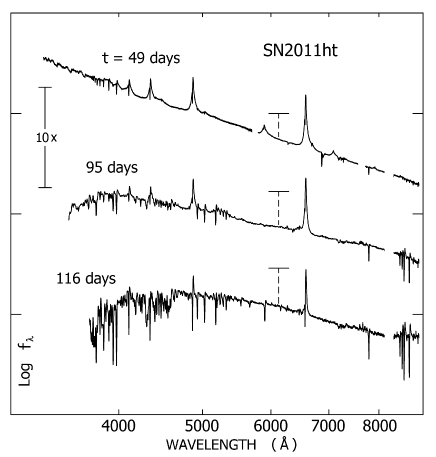
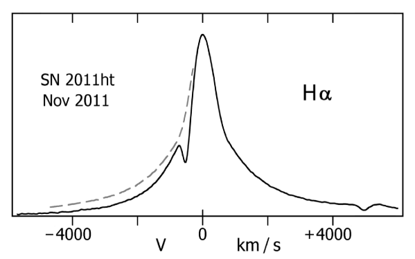
An excellent example is SN2011ht Roming et al. (2012); Humphreys et al. (2012), whose brightness and timescale resembled a supernova (Figure 2). It may have been either a supernova impostor or else a true SN within a dense envelope of prior ejecta (Section 5.4 below); but in either case the observed display was a radiation-driven outflow. Its spectrum (Figure 3) had characteristics explained in Section 4 below, with outward speeds of several hundred km s-1 and no hint of a blast wave before the brightness declined. Broad emission line wings were caused by Thomson scattering rather than bulk motion (Section 4.2), and the kinetic energy of visible ejecta was much smaller than in a normal SN Humphreys et al. (2012).
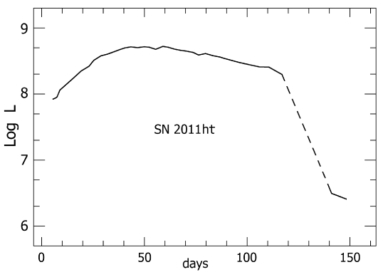
About two months after maximum, the visual-wavelength brightness of SN 2011ht abruptly decreased by a factor of 60 (Figure 2). Since normal dust formation does not account for this change Humphreys et al. (2012), the simplest interpretation is that most of the trapped radiation escaped through the photosphere just before that time. A normal core-collapse supernova would have remained substantially brighter due to radioactive decays in the ejecta. Some authors assumed that 2011ht was a supernova in a discussion of the light curve Mauerhan et al. (2013); but the lack of a radioactive afterglow was decidedly peculiar in that case, and the light curve was reasonable for a non-SN instability (Section 5 below). The spectra in Figure 3 gave far more definite information than the light curve did, and strongly implied an opaque continuum-driven outflow far above the Eddington Limit Dessart et al. (2009); Humphreys et al. (2012); Kankare et al. (2012).
Historically, the first observed giant eruption was P Cygni about 400 years ago Weis & Bomans (2020); de Groot & Sterken (2001_); Humphreys et al. (1999). Its maximum luminosity was of the order of , quite small by giant eruption standards; but, unlike normal LBV events, that amount significantly exceeded the quiescent brightness. P Cyg’s outburst (actually two or more episodes) persisted for years so the radiative energy output was probably more than ergs. Today this star is located in the LBV instability strip in the HR Diagram, but it has not exhibited an LBV event. Possibly this is a hint that the interval between episodes is related to the strength of the most recent instance, analogous to some forms of relaxation oscillators.
Among the eruptors discovered since 2000, some had luminosities comparable to Car and/or P Cyg, but behaved very differently. SN2000ch, for instance, has exhibited multiple outbursts considerably brighter than the familiar type of LBV outburst, but not as bright as Car’s Great Eruption Wagner et al. (2004); Pastorello et al. (2010); van Dyk et al. (2013). Those events were hotter than an LBV outburst, with higher outflow speeds, much shorter durations, and the luminosity may have increased appreciably on each occasion. Altogether its behavior differs from LBV’s, Car, and the brighter giant eruptions noted below. P Cyg might have appeared similar in the years 1600–1650, but this is merely a speculation.
A more extreme object with a different kind of multiplicity was described in Humphreys et al. (2016). PSN J09132750+7627410, a SN impostor in NGC 2748, attained a luminosity of the order of , comparable to Car’s maximum, for several months—even though its quiescent luminosity was probably less than . Near maximum its spectrum resembled SN2011ht described above. Its chief peculiarity was the existence of several distinct outflow velocities in each absorption feature: , , and km s-1. These may signify either a series of mass-loss episodes, or structure in the observed episode, or separate ejecta from more than one star. The two larger speeds are much faster than an LBV outflow. Multiple velocities have been seen in a few other eruptive stars—e.g., see Margutti et al. (2014); Mauerhan et al. (2015).
Two pre-2000 giant eruptions, SN1954J Tammann & Sandage (1968) and SN1961V Zwicky (1965); Humphreys et al. (1999), have had enough time to show whether their stars survived. The SN1954J event had a maximum luminosity of the order of with a duration less than a year Van Dyk (2005); Van Dyk & Matheson (2012); Humphreys et al. (2017). The surviving star, a.k.a. V12 in NGC 2403, has a likely mass around 20 and is seriously obscured by circumstellar dust. Its spectrum includes Thomson-scattered emission line profiles, indicating a present-day opaque outflow (Section 4.2 below). This fact is strong evidence that the observed object really is the survivor of a giant eruption. The star was probably in a post-RSG state when the event occurred Humphreys et al. (2017). SN1961V, on the other hand, remains doubtful. It achieved a peak luminosity well above with an overall event duration longer than a normal supernova, but no survivor has been identified with high confidence Kochanek et al. (2011); van Dyk & Matheson (2012).
An unexpected development since 2000 has been the occurrence of precursor eruptions—i.e., giant eruptions that were followed several years later by real supernova events. At first sight this seems unlikely, because the final stages of core evolution have timescales of days, hours, and minutes rather than years. A few years is a likely timescale in the outer layers (Section 5 below), but in the standard view those regions “don’t know” the precise state of the core. Hence one might conclude that precursor events arise in or near the core; but that assessment is too glib to be entirely satisfying, as noted in Section 5 below. The most notorious example of this phenomenon was SN 2009ip, whose blast wave explosion was not observed until 2012 Margutti et al. (2014). That object exhibited other events between 2009 and 2012. Evidently some part of the star became unstable a few years before the SN event, but then the observed timescale didn’t accelerate with the core evolution. Or perhaps the 2012 shock wave did not represent the real terminal event Pastorello et al. (2013); Fraser et al. (2013a)! See comments in Section 5.3 below.
SN 1994W, SN 2009kn, and SN 2011ht probably ejected material months or years before their terminal explosions Dessart et al. (2009); Humphreys et al. (2012); Fraser et al. (2013b). Since those objects became strangely faint at the stage when 56Ni decay normally produces luminosity after a core-collapse SN event, some authors suspect that core collapse did not occur—e.g., Dessart et al. (2009).
Giant eruptions are usually easy to distinguish from LBV events. They have far greater mass loss rates, substantial increases in luminosity, and shorter durations in most cases. A few LBV’s, however, have mistakenly been given SN designations. SN 2002kg, for example, is a luminous LBV also known as V37 in NGC 2403 Weis & Bomans (2005); Van Dyk (2005); Humphreys et al. (2017).
3.3 Eta Carinae
The classic example of a supernova impostor, of course, is Carinae. It merits a separate subsection here, because it has been observed in far more detail than any other relevant object. Following the tradition of classic examples in astronomy, it has abnormal properties. Its event seen in 1830-1860 persisted much longer than other known giant eruptions, and it has a companion star that approaches rather closely at periastron. Many authors reviewed Car in ref. Davidson & Humphreys (2012), and later developments have not altered the main facts.
The star’s luminosity is roughly (Figure 1). Before 1830 its mass was probably in the range 140–200 , with an apparent temperature close to 20,000–25,000 K Davidson (2012). Then its 30-year Great Eruption ejected 10-40 at speeds averaging 500 km s-1. It converted more than ergs of energy to roughly equal portions of radiation, kinetic energy of ejecta, and potential energy of escape. The resulting “Homunculus” ejecta-nebula Smith (2012) is famously bipolar, indicating a complex role for angular momentum Davidson (2012). The ejected material is clearly CNO-processed, with helium mass fraction 0.4–0.6 Davidson et al. (1986); Dufour et al. (2001). The star’s subsequent recovery has been unsteady, including a smaller eruption around 1890 and two later disturbances Davidson (2012); Humphreys et al. (2008); Humphreys & Martin (2012). Until recently its wind was opaque in the continuum with y-1, and most likely above y-1 a century ago Humphreys et al. (2008). That rate was too large for a line-driven stellar wind.
The companion object is most likely an O4-type star with a highly eccentric 5.54-year orbit, see many articles in Davidson & Humphreys (2012). The primary star is indeed the eruption survivor, since it has an extremely abnormal wind that has been diminishing since the event. But the hot secondary star alters the situation in several ways.
-
•
It ionizes much of the primary wind, greatly affecting the observed spectrum.
- •
-
•
Tidal friction near periastron can transfer orbital angular momentum to the primary star’s outer layers. If so, the equilibrium rotation period would be in the range 50-150 days. The primary star may be highly vulnerable to tidal effects because it is close to the Eddington Limit, but this possibility needs a careful quantitative analysis (see Section 6 below).
-
•
Many authors have noted that the companion star may have triggered the Great Eruption via tidal influence near periastron Davidson (2012); but we must not confuse a trigger with the instability mechanism. Perhaps the nearly-unstable primary star gradually expanded until the other star’s tidal influence tipped it over the edge. But this idea is not simple, since there is evidence for earlier episodes Davidson & Humphreys (1997); Weis (2012) and the present-day orbit eccentricity is too large to be caused entirely by the 19th-century mass loss Davidson (2012); Davidson et al. (2017). Incidentally, the present-day orbital period cannot be used to estimate periastron times for the era of the Great Eruption. If we try to extrapolate back to about 1840, the gradual period change due to fluctuating mass loss causes a phase uncertainty of the order of a year.
-
•
The companion star may be the main reason why Car’s eruption was fainter and more protracted than most supernova impostors Davidson (2012). For several years the second star was inside the radius of the eruption photosphere, and near periastron it may have stirred the instability. During the great eruption, and for many years afterward, the secondary star probably accreted some material from the primary’s outflow Soker (2005, 2007); Kashi & Soker (2009); Humphreys et al. (2008); Davidson (2012); Davidson et al. (2015). Possible consequences for the orbit have not yet been examined.
-
•
As noted in Section 6 below, various authors have speculated that Car was originally a triple system and two of the stars merged. Models of that type have a large number of assumed parameters, they do not agree with each other, and there is no evident need for a third star.
For historical reasons Humphreys & Davidson (1979), Car is often called an LBV despite its location in the HR Diagram (Figure 1). The high-luminosity end of the LBV strip in Figure 1 may be misleading, and in principle every star with and 25000 K might be an LBV; there are not enough examples to know. But that is only a possibility, and we have no definite reason to classify Car as an LBV. An LBV-like eruption would be complicated for this object, because the radius of a 10000 K photosphere would exceed the companion star’s periastron distance.
4 The Spectrum of an Opaque Outflow
This section has four main points: (1) Giant stellar eruptions usually have similar colors and spectra even if they’re caused by different processes. (2) A particular type of emission line profile indicates an opaque outflow. (3) Stellar spectral types are not reliable indicators for outflow temperatures. (4) LBV outflows are not homologous with giant eruptions.
4.1 The Continuum
The apparent radiation temperature of an opaque outflow can be defined in various ways—e.g., based on the photon-energy distribution of the emergent continuum, or its slope at selected wavelengths, or on subsets of absorption features, etc. These alternative ’s can differ by 20% or more, leading to confusion when one attempts to compare values quoted in papers. “Effective temperature” used for stellar atmospheres is not appropriate, because an outflow has no fundamental reference radius that is meaningful for that purpose. Also note that an optical depth value of 2/3 has no significance in this context. (Regarding photon escape probabilities, 1.0 to 1.3 in a diffuse spherical outflow corresponds to in a plane-parallel atmosphere.)
And we must be careful with the word “photosphere.” The region with optical depth has little effect on an outflow’s emergent photon energy distribution, because the dominant opacity is usually Thomson scattering by free electrons. That process has only a weak effect on photon energies. Consider instead a deeper region where absorption and re-emission events are frequent enough to establish . Outside some radius , the average photon escapes via multiple scattering before it experiences an absorption event. Evidently the emergent photon energy distribution depends mainly on temperatures that exist just inside radius . In this overview “photosphere” means that region.
Classical diffusion theory gives the approximate size of Rybicki & Lightman (1979); Davidson (1987b). Suppose that local opacities for absorption, scattering, and their sum are , , and , averaged over photon energies in some optimal way. Define a “thermalization opacity”
| (1) |
with associated optical depth
| (2) |
Often called thermalization depth or diffusion depth, is typically of the order of in a giant eruption or an LBV event photosphere. Calculations show that is approximately the radius where Rybicki & Lightman (1979); Davidson (1987b), and we can regard the photosphere as the region where . This is not a formal statement, but in practice it applies for any reasonable density law and for large as well as small opacity ratios . The emergent continuum is created mostly at to 2.0, while absorption and emission lines are formed mainly at or perhaps . If and are the temperatures at 1 and 2, then we can liken to the of a star with a similar spectrum, though their values may disagree because they are defined differently. (Caveat: In published models of opaque winds, some authors define the photospheric radius by or even , rather than . With those choices, a quoted “photosphere temperature” is cooler than the emergent distribution of photon energies.)
In a simple model where opacity depends only on and , the temperature at a given location depends approximately on two quantities, and where is the local outflow velocity Davidson (1987b); Owocki & Shaviv (2016). Figure 4 shows examples of and in spherical outflows. Corresponding radii are shown in Figure 5. These sketches are intended only for conceptual purposes; they are based on simplified models that ignore some major details (see below).
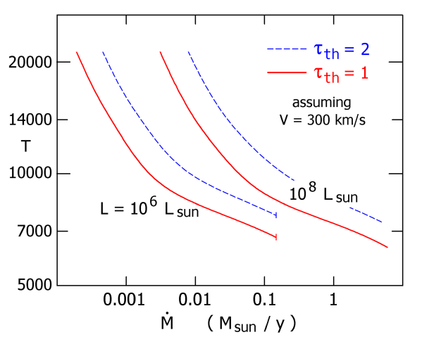
With Figure 4 in view, imagine a case with constant luminosity while gradually increases. Initially the flow is transparent so our model does not apply. But when becomes large enough to be opaque, then it determines the apparent temperature. Increasing causes the photosphere to move outward, and roughly as shown in the upper half of Figure 4. Below 9000 K, however, the proportionality changes to because the opacities decline rapidly. K requires a very large flow density. As noted above, is a fair indicator of the absorption and emission lines – except for a caveat in Section 4.3 below.
(This paragraph concerns technicalities that don’t affect the main concepts.) Each temperature in Figure 4 refers to a location in the flow, which does not represent any specific observable quantity. For comparison with observations, one would need to calculate emergent radiation in a manner resembling Davidson (1987b) and Hummer & Rybicki (1971); but a model with wavelength-dependent opacities would be much better. Figure 4 is based on many simplified models with constant luminosities , mass-loss rates , and flow velocities . It was assumed that , with LTE Rosseland mean opacities which are readily available (http://cdsweb.u-strasbg.fr/topbase/, Badnell et al. (2005), and refs. therein). Hydrogen and helium mass fractions were and . Integrating the spherical radiative transfer equations Hummer & Rybicki (1971) with those opacities, we can calculate . One recent analysis Owocki & Shaviv (2016) appears at first sight to favor lower temperatures than Figure 4, but the differences involve merely the distinction between and , and varying definitions of the observed . True ionization in the outer regions tends to be larger than the LTE values; if so then the temperatures in Figure 4 are overestimates. Errors of that type are probably comparable to the differences between alternative definitions of for the emergent radiation.
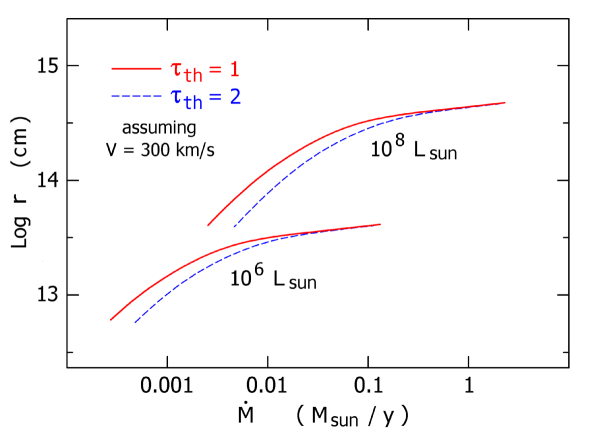
Figure 4 is fairly consistent with observed giant eruptions, such as Car marked in Figure 1. Exceptionally high flow densities occurred in Car’s 1830–1860 Great Eruption, with y-1 and Davidson & Humphreys (2012); so it should have had exceptionally low photospheric temperatures. Reflected light echos provide spectra of that event Rest et al. (2012); Prieto et al. (2014); Smith et al. (2018a). The light-echo researchers deduced a temperature near 5000 K, but that was an informal value, not well-defined and not based on a quantitative analysis. Judging from the published description and reasons noted in Section 4.3 below, the spectrum most likely indicated 5500 to 6500 K in Figure 4 Davidson & Humphreys (2012b). (Recall that denotes the temperature at a particular location in the outflow, not an emergent radiation temperature.) If we define “apparent temperature” in a different way, its value may have been as low as 5000 K Owocki & Shaviv (2016). A second, lesser eruption of Car in the 1890’s had K, according to the earliest spectrogram of this object Humphreys et al. (2008). Several extragalactic giant eruptions have been observed since 2000, usually showing K (Section 3.2 above). LBV outbursts have much smaller luminosities, and usually reach 8000-9000 K like AG Car in Figure 1. The assumptions in Figure 4 are not valid for them, because their photospheres are not located in the high-speed part of the flow (Section 4.5 below). However, those observed minimum temperatures of LBV’s are very likely determined by the rapid decline of opacity below 9000 K, even though the photospheres resemble static atmospheres.
In summary, there is no known observational reason to doubt the general appearance of Figure 4 for opaque radiation-driven outflows.
4.2 Distinctive Emission Line Profiles
The brightest emission lines from an opaque outflow generally have a certain type of profile, illustrated in Figure 6. Smooth broad line wings extend beyond km s-1 even though the wind speed is less than 700 km s-1; and the longer-wavelength side is stronger. These are classic signs of Thomson scattering by free electrons Weymann (1970); Davidson et al. (1995); Chugai (2001); Dessart et al. (2009); Humphreys et al. (2012). Since the electrons have r.m.s. thermal speeds of the order of 600 km s-1, some of the photons acquire large Doppler shifts in multiple scattering events before they escape. Meanwhile, expansion of the outflowing material favors shifts toward longer wavelengths. Obviously the resulting profile depends on , the line-emitting region’s average optical depth for Thomson scattering. The shape in Figure 6 indicates 0.5 to 2, and appears to be generic. It specifically represents SN 2011ht Humphreys et al. (2012), but SN 1994w exhibited a similar H profile, and so do other giant eruptions and Car’s dense wind Dessart et al. (2009); Humphreys & Martin (2012); Mehner et al. (2015).
The moderate size of has a simple explanation. In typical eruptions with K, 1 to 2 —a consequence of atomic physics. Hence the continuum photosphere boundary automatically has 1 to 2. Since the emission lines are formed outside the photosphere, we therefore expect , or perhaps a little smaller, for bright emission lines. The main point here is that an observed profile like Figure 6 is good evidence for an opaque or semi-opaque outflow. It recognizably differs from emission lines seen in normal stellar winds, expanding shells, nebulae, and supernova remnants.
(Caveat: In some papers a Thomson-scattered line profile is called “Lorentzian,” often without recognizing its significance. That usage gives a flatly wrong impression in two respects. First, in physics the word “Lorentzian” has very specific connotations: the Fourier transform of an exponential decay, the natural shape of an idealized spectral line, closely related to the uncertainty principle. None of these applies to the shape in Figure 6. Second, the wings of a true Lorentz profile are like but the wings of a Thomson-scattered profile are like . This difference is fundamental, not just a matter of opinion.)
4.3 Cautionary Remarks about Absorption Features
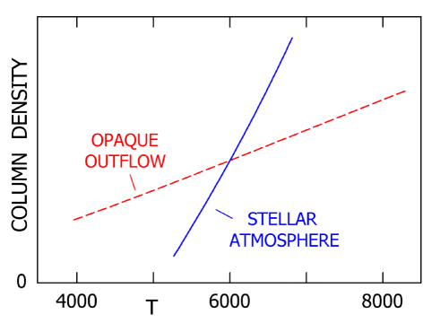
An opaque outflow also produces absorption lines, but they cannot safely be compared with stellar spectral types. The most dramatic example concerns Car’s Great Eruption. Spectra of that event have been obtained via light echos, leading to an estimate K which seemed to contradict an expected value of 7500 K Rest et al. (2012); Prieto et al. (2014); Smith et al. (2018a). But that conclusion had two disabling flaws. (1) In fact the expected value was far below 7500 K Davidson (1987b); Davidson & Humphreys (2012b); Owocki & Shaviv (2016). (2) More pertinent here, spectral classification standards for stars do not apply to a mass outflow. For instance the light-echo spectra of Car’s Great Eruption showed absorption features of CN, which would indicate K in a star—but they may occur in an outflow with K.
Figure 7 shows why. Each curve represents the column density of material cooler than . A stellar amosphere with K has almost no material below 5000 K, but a diffuse outflow with K can have an appreciable amount of cooler gas at large radii. This difference is a consequence of two facts: (1) the mass distribution in an outflow resembles a power law instead of the exponential that roughly describes a stellar atmosphere, and (2) Radiation density in an outflow has a “dilution factor.” Figure 7 is merely schematic, but it suggests that an eruption with K can form cool spectral features such as CN in its outer regions. Absorption lines formed at smaller radii may be good indicators of , but they must be chosen carefully. Since LTE is a poor approximation for , and there are other complications, a realistic model of the absorption line spectrum will be extremely complex (see below). Meanwhile, so far as available information allows us to judge, the light-echo spectra of Car’s eruption appear consistent with standard portrayals of that event.
4.4 Why a Real Outflow Spectrum is Exceedingly Difficult to Calculate
The dependence of on was first described long ago Davidson (1987b). Figure 4 and ref. Owocki & Shaviv (2016) employ modernized opacities, but the resulting quantities are highly imprecise because the models are highly simplified. A truly realistic calculation must include all of the following complications.
-
1.
Real opacities depend on photon energy, and no form of average over is fully consistent with all of the radiative transfer equations. The model should include -dependences.
-
2.
Standard LTE opacities are very unreliable in the region with , because it is far from thermodynamic equilibrium. Existing NLTE codes do not adequately include some effects, e.g., items 4 and 5 below.
-
3.
A realistic model needs a good velocity law , and the functional form used for line-driven stellar winds is probably wrong for an opaque flow. A valid is surprisingly difficult to calculate, because of item 4 below Shaviv (2000); Owocki & Shaviv (2012); Guzik (2018). This fact becomes even worse when we note that opacities due to Fe+ and other complex species depend on many spectral lines whose interactions depend on item 4 as well as !
-
4.
A radiation-driven outflow is obviously unstable—“a light fluid pushing a heavier one”—and breaks up into condensations, greatly complicating the radiative transfer problem Shaviv (2000, 2001); Owocki & Shaviv (2012). Modern codes employ a position-dependent “clumping factor” (e.g., Groh et al. (2011)) which entails several assumptions and free parameters that are very uncertain. Hence the resulting models are useful guides but there is no reason to assume that they are correct. If each condensation is not transparent, then radiation tends to escape via the easiest paths between condensations. (This definitely happened in Car’s giant eruption Shaviv (2000).) The words “porosity” and “granulation” are often used in this context. Results depend on the condensation sizes, densities, and even shapes. A practical technique, analogous to mixing length theory for convection, is needed for inhomogeneous radiative transfer. Perhaps a recipe can be developed from a large number of specialized three-dimensional simulations. See Guzik (2018); Owocki et al. (2019).
-
5.
As Car notoriously shows, spherical symmetry may be a poor approximation. Moreover, since a spherical model maximally entraps the radiation, it represents an extreme case, not typical or average. And the spectrum of a non-spherical outflow depends on the observer’s viewing direction.
Omitting any of these complications may cause the results to be almost as inaccurate as the simplified models in Figure 4. Some existing codes employ elaborate radiative transfer with some NLTE effects, but there are reasons for skepticism. Items 3, 4, and 5 have multiple undetermined free parameters, not advertised in most research papers. Items 3 and 4 acting together may invalidate the radiative transfer methods for spectral lines. Most important, the realism of a calculation is very difficult to test. Approximately matching an observed spectrum does not prove correctness, since there are enough free parameters to compensate for omitted effects. In summary, existing codes illustrate most of the chief processes, but they must not be regarded as decisive or authoritative. Their uncertainties may be far worse than most authors assume.
4.5 Are LBV’s Relevant?
As noted at the end of Section 3.1 above, the most critical mass-loss episode may conceivably occur just before the LBV stage of evolution. If so, then the relatively modest, familiar type of LBV event might have little in common with continuum-driven giant eruptions.
The fast region of any LBV wind (usually 100 to 300 km s-1) is transparent in the visual-wavelength continuum. This fact was noted before 1990 Davidson (1987b), and later motivated the static atmosphere models Leitherer et al. (1989); de Koter et al. (1996); Groh et al. (2011); Gräfener et al. (2012); Sanyal et al. (2015). But it doesn’t necessarily apply to the inner, slow, denser part of the outflow during a major LBV event. The following remarks concern major LBV1 eruptions with 10,000 K, not the states above 15,000 K that are emphasized in most analyses since 2010.
Recall the analogy between a stellar wind and flow through a transonic nozzle, with , the speed of sound, at radius Shore (1992); Lamers & Cassinelli (1999). The subsonic region resembles an atmosphere constrained by gravity, while the flow dominates outside . Imagine such a hybrid model of AG Car’s major eruption around 1994, when declined to about 9000 K while rose to about y-1 Stahl et al. (2001). At that time km s-1 in the photosphere, and the photospheric outflow speed was of the order of . The sonic point was thus two or three scale heights above the photosphere, much closer than in a normal line-driven stellar wind. According to Figure 4, a larger value of would have moved the photosphere to the sonic point – so a flow model rather than a static atmosphere would have become appropriate if had grown above that amount. In this order-of-magnitude sense the major eruption was “almost” opaque.
A normal line-driven stellar wind has an indirect relation to the continuum photosphere, with in the photosphere. The much larger in major LBV eruptions, along with proximity to the Eddington Limit, suggests that their outflows are more directly related to their continuum photospheres. This line of thought—or rather, of surmise—motivates a three-step conjecture:
-
•
The rapid decline of opacity for K encourages the eruptive photosphere to choose a temperature near that value. In other words, for a case with , the basic parameters of the subphotospheric inflated region would need to become unreasonable in order to push substantially below 8000 K.
-
•
Due to the role of continuum radiation in the initial acceleration, the sonic point is related to the photosphere. Consequently the outflow speed at is where is of the order of 0.1.
-
•
Therefore, at times when K, .
This is an empirical hypothesis, not a theoretical prediction. There are semi-theoretical methods of predicting LBV mass loss rates, far more elaborate than this reasoning, but their developed versions have been applied mainly to the hotter states above 15,000 K Vink (2018). Anyway, the above expression is fairly consistent with estimated values for major LBV1 eruptions.
If we portray LBV outbursts as quasi-static inflated states Leitherer et al. (1989); de Koter et al. (1996); Gräfener et al. (2012); Sanyal et al. (2015), then unfortunately we de-emphasize the mass outflow. Since the latter is probably more consequential, the “eruption” aspect expresses a broader significance than the inflation. On the other hand, it is conceivable that most of the cumulative LBV mass loss occurs in rare giant eruptions à la P Cygni, not merely major eruptions. In any case the static 1-D models do not answer the main questions, Section 5.1 below.
5 Physical Causes of the Eruptions
The Eddington Limit turns out to be wonderfully subtle and complicated. Relevant instabilities were recognized after 1980 (see many refs. in Humphreys & Davidson (1994)), but they’re difficult to analyze or even to describe. Practically all of our knowledge of eruption parameters, post-eruptive structure, timescales, and long-term mass loss is still empirical.
Two classic high-mass stellar instabilities were naturally suspected when giant eruptions and LBV events attracted notice in the 1980’s: The Eddington mechanism or Ledoux-Schwarzschild instability energized in the stellar core Schwarzschild & Härm (1959), and radial dynamical instability which occurs if the average adiabatic index falls below 4/3 Stothers (1999). But they proved unsuitable Glatzel (2005), and have been replaced by newer ideas which are generally non-adiabatic, involve radiation pressure, and resemble each other. Three regions in the star merit special attention: the photosphere, the “iron opacity bump” region with 200,000 K, and the stellar core, broadly defined.
Details of the instabilities are too lengthy to explore here. Instead, this overview lists a set of essential considerations, including some that have seldom been discussed in research papers. Here rotation does not get the attention that it deserves, because that would greatly lengthen the text. Interacting or merging binary scenarios are omitted because there is no clear need for them at this time, see Section 6.
5.1 The Modified Eddington Limit
Giant eruptions exceed the Eddington Limit. Thus it seems natural to guess that the progenitor stars were very massive, close to the Limit, and vulnerable to the same instabilities as LBV’s. This connection between LBV’s and giant eruptions may be illusory, but thinking about it leads to some useful ideas.
Observed ratios are clues to the LBV phenomenon in two different ways. First, of course, their proximity to the Eddington Limit (Section 3.1 above) implies a large role for radiation pressure. Second and less obvious, the distinction between two classes of LBV’s favors an instability in the outer layers, not the stellar core. Types LBV1 and LBV2 have different central structures because they represent different stages of evolution (Section 3.1 above and Humphreys et al. (2016)). The stars’ outer 3% of mass, however, have similar radiation/gas ratios for both classes, and similar variations of opacity.
In the classical Eddington Limit
| (3) |
the opacity includes only Thomson scattering by free electrons. Absorption opacity practically vanishes as a static photosphere approaches the Limit, because density becomes very low. The classical Eddington parameter can thereby approach 1 in an old-fashioned radiative atmosphere model. However, the photospheric may be appreciable in a model with 0.95, and deeper layers may have larger opacities in any case. During the 1980’s this thought inspired the idea of a “Modified Eddington Limit” that takes into account Humphreys & Davidson (1984); Appenzeller (1986); Lamers (1986); Davidson (1987a); Appenzeller (1989); Humphreys & Davidson (1994); Asplund (1998). It was an empirical hypothesis, not a theoretical prediction, motivated by Car and observed LBV behavior.
In principle there are two forms of Modified Eddington Limit. (1) It might be a well-defined limit to the allowed values of in a static stellar model, like the classical limit but including realistic , convection, incipient porosity, etc. (2) Or, more likely, it may signify an instability that arises when exceeds some value, see Section 5.2 in Humphreys & Davidson (1994). In either case the critical depends on opacities in the outer 3% of the star’s mass, or maybe the outer 1%.
Rapid rotation reduces the effective gravity mass, thereby altering any form of Modified Eddington Limit. The terms “ limit” and/or “ limit” allude to this obvious fact, but the implications are often oversimplified. Two decidedly non-trivial subtleties occur: (1) Rotation causes a star’s subsurface temperatures to depend on latitude. Resulting alterations of opacity affect the topics of Section 5.2 and 5.3 below. (2) The specific angular momentum expelled in a giant eruption may be either larger or smaller than in the lower layers. Consequently the effects of rotation may evolve during the eruption Davidson (2012).
5.2 The Photosphere, Bistability, and Surface Activity
The easiest place to start is the photosphere. Traditionally, the total energy flow in a stellar interior can exceed by inciting convection Joss et al. (1973). But convection becomes inefficient in the photosphere, so radiation must carry nearly all of the energy flux there. Imagine a static model wherein increases inward, and radiative forces are less than gravity outside some radius . Inside , convection carries the excess energy flux. But an increase in would presumably cause to move outward relative to the stellar material. For some value of , moves into the photosphere; so there may be a practical limit, somewhat smaller than . By extrapolating normal atmosphere models, one can identify a limiting around Lamers & Fitzpatrick (1988); Gustafsson & Plez (1992); Ulmer & Fitzpatrick (1998). But the reasoning is dangerously subtle, and a different approach suggests that a star may become unstable at a smaller value of , see below.
Next, instead of the above view, suppose that “Modified Eddington Limit” connotes an instability that arises somewhere in the range , rather than a well-defined static limit. At relevant photospheric densities, has a maximum in the vicinity of K, involving the ionization ratio Fe++/Fe+. Thus a high- atmosphere may be very unstable in a particular range of around that maximum, and might act as a relaxation oscillator jumping back and forth across the unstable range Appenzeller (1986, 1989).
Behavior like that is observed at a somewhat higher temperature Pauldrach & Puls (1990); Lamers et al. (1995); Vink et al. (1999); Vink (2012). Consider a standard hot line-driven wind model wherein the star gradually becomes cooler. As declines below 20000 K, Fe++ and other suitable ion species become numerous enough to drastically increase ; so the wind becomes slower and much denser. The transition occurs across a narrow range of , hence the term “bistability jump.” It was noted around 1990 as a likely cause of LBV events Pauldrach & Puls (1990); Lamers et al. (1995). That idea originally meant a difference between two outflow states, but it rapidly evolved into a bistability between two quasi-static states of the star’s outer layers Leitherer et al. (1989); de Koter et al. (1996); Groh et al. (2011); Gräfener et al. (2012); Sanyal et al. (2015). One state corresponds to a quiescent LBV, the other occurs during an LBV eruption, and intermediate states are more unstable due to the opacity maximum mentioned earlier. In the eruptive state, the outer layers are greatly expanded or “inflated.”
But a set of inflated and non-inflated models does not constitute a theory of LBV variability; instead it plays a role more like an existence theorem in mathematics. A proper theory must address the following questions.
-
1.
What is the state of the outer regions during a major event when 10000 K? The most elaborate spectral analyses Groh et al. (2011); Gräfener et al. (2012) focus instead on models with 15000 K, close to the bistability jump. The cooler state is more difficult but also more consequential. Moreover, all 1-D models disallow some effects that are probably essential Jiang et al. (2018).
-
2.
Why and when does an LBV eruption end? The star does not merely evolve into an inflated state and remain there until further evolution occurs. Instead it jumps unpredictably back and forth between differing states. Does a major LBV event cease when a critical amount of mass or energy or angular momentum has been lost, or are the reasons chaotic or related to inconspicuous changes in the stellar interior?
-
3.
Is the photospheric opacity behavior sufficient to cause an LBV event? Or is the deeper iron opacity peak (Section 5.3 below) needed?
-
4.
The central LBV problem concerns mass loss, not the star’s radius. What factors determine the increased ? Do they resemble the conjectures in Section 4.5 above? Conventional line-driven wind theory is probably inadequate in this parameter regime (Section 4.4 above). A Monte Carlo radiative transfer technique predicts credible values for LBV’s in their hotter phases Vink (2018), but it omits many intricate effects seen in a 3-D simulation Jiang et al. (2018).
-
5.
What determines the event recurrence rate? Is it like a relaxation oscillator wherein the recurrence time depends on details of the preceding event Appenzeller (1986, 1989), or is there some form of periodicity? P Cyg had an extremely large event 400 years ago and has seemed quiet ever since de Groot & Sterken (2001_).
-
6.
What determines the timescale of a transition to the LBV-event state? Is it a thermal timescale for some relevant set of outer layers?
-
7.
How large is the cumulative amount of mass loss? Does it vary greatly or randomly among LBV’s with a given luminosity?
-
8.
How strongly do these answers depend on rotation as well as chemical composition? And how much do the LBV eruptions alter the surface rotation and composition?
-
9.
Do more extreme LBV eruptions occasionally occur, violent enough to substantially increase the luminosity while ejecting far more mass than usual? Observed ejecta nebulae, e.g., around AG Car, may be relics of such events. They might account for most of the cumulative mass loss.
The last item pertains to giant eruptions. In order to expel a mass which greatly exceeds that of the unstable region, the process must be like a geyser: instability begins at the top and moves downward (relative to the material) until some factor stops it. In this way a photospheric instability might even cause a giant eruption. As outer layers depart, a large reservoir of radiative energy is progressively uncovered. At any given time the configuration resembles a steady-state model, since the observed timescale is much longer than the dynamical timescale. Presumably the eruption ends when conditions change at the base of the flow – perhaps when it reaches some particular feature in the pre-eruption interior structure.
Another form of Modified Eddington Limit relates to dynamical processes rather than the temperature dependence of opacity. A static atmosphere dominated by radiation pressure tends to develop inhomogeneities, granulation, and porosity like an outflow; see Shaviv (2001); Owocki & Shaviv (2012) and many refs. therein. Resulting turbulence can engender MHD effects, even though the photosphere is well above the temperatures traditionally associated with stellar activity. These phenomena may influence the outflow rate, and might even determine it. Conceivably, Car’s dense wind a century ago Humphreys et al. (2008) may have involved stellar activity analogous to a red supergiant! Cf. Jiang et al. (2015).
Most of the above possibilities are not mutually exclusive.
5.3 The Iron Opacity Peak
The “iron opacity peak” locale in a star, described below, is probably crucial; but its instabilities are too complex for simple analysis, math expressions, and predictions. A decisive analysis will require numerous 3-D simulations which have not been feasible so far.
Absorption opacity has a dramatic maximum at temperatures around 180,000 K, for reasons concerning ionization stages of iron. In a typical LBV-like very massive star, throughout a temperature range such as 100,000 to 300,000 K, though the actual limits depend on mass density. Vigorous convection occurs there because obviously exceeds , if signifies the total energy flow. Such a region offers a zoo of instabilities, and dynamically it decouples the outer layers from the stellar interior. Since the associated mass and energy greatly exceed the photosphere, this region is the most promising part of the star for eruption mechanisms. Its usual name, the iron opacity peak zone, might be confused with the iron peak of cosmic abundances; and “iron opacity bump zone” is both inelegant and cumbersome. For convenience we’ll use an acronym here: OPR = iron opacity peak region in the star. Although it usually occurs in the outer 1% of the star’s mass distribution, its spatial radius may be considerably smaller than the stellar radius . A second opacity peak will also be mentioned, involving helium at lower temperatures.
The OPR mass and energy are difficult to estimate from observational data. If is the mass column density of layers cooler than , and radiation pressure dominates, then so
| (4) |
where is a radius that has temperature . But the factor is quite uncertain, because may lie deep within an extended envelope. Consider, for instance, Car before its giant eruption. If we know only that , , and 20,000 to 25,000 K Davidson (2012), then the mass in the temperature range 100,000–300,000 K may have been anywhere in the range 0.002 to 0.1 . The thermal timescale for this OPR might have any value ranging from a few days to a few months, depending partly on how we define it. Given these strong dependences, the effects of OPR instabilities may be very sensitive to the evolutionary state and structure of the star—and thus consistent with observed facts about giant eruptions and LBV’s.
A standard LBV eruption might expel no more than the OPR mass, and the two amounts may even be related. But a giant eruption rooted in that region must be geyser-like (Section 5.2). Some forms of instability cannot easily function like geysers, for reasons involving timescales – see a remark later below.
Since 1993, almost every stability analysis of very massive stars has emphasized “strange modes” of pulsation Gautschy & Glatzel (1990); Glatzel & Kiriakidis (1993); Stothers & Chin (1993); Glatzel (2005); Saio (2009); Guzik & Lovekin (2014); Lovekin & Guzik (2014a); Guzik et al. (1999). Apart from mathematical details, they have the following attributes.
-
1.
Strange modes are essentially dynamical rather than thermal. They resemble accoustic waves, in contrast to thermodynamic Carnot-cycle pulsations driven by the mechanism in lower-mass stars.
-
2.
Hence they are fundamentally non-adiabatic. They become especially strong if the local thermal timescale is shorter than the dynamical timescale.
-
3.
They occur if radiation pressure exceeds gas pressure.
-
4.
The density dependence of opacity, , is more critical than .
-
5.
Purely radial strange modes can occur, but non-radial modes may be more important.
These characteristics are almost perfectly suited to the OPR in a star near the Eddington Limit. Item 3 causes the local mass density to be relatively low, thereby enabling item 2. For a very brief account of strange modes, see Saio (2009).
Altogether, then, in a star near the Eddington Limit, the OPR forms a queasy sort of cavity between the stellar interior and the outer layers—with strong consequences for pulsation modes. Even if we consider only 1-D radial motions, gas-dynamical simulations reveal phenomena that appear crucial for LBV’s and giant eruptions Lovekin & Guzik (2014a); Guzik (2018); Guzik & Lovekin (2014); Lovekin & Guzik (2014b); Onifer & Guzik (2005). An essential factor is the time dependence of convection. Normally a massive stellar interior obeys the Eddington Limit by shifting some of the energy flux to convection where necessary Joss et al. (1973). But this assumption fails in a structure that changes rapidly, e.g., in pulsating layers. Convection needs some time to develop, and the dominant convective cells have finite turnover times. Hence the convective energy flux lags behind the total energy flux, especially in the circumstances listed above for strange modes. As explained in the papers cited above, this fact causes the radiative flux to exceed the Eddington Limit at some times and places in a pulsation cycle. No actual runaway outburst occurred in the simulations, but their boundary conditions and lack of non-radial modes tended to inhibit such a development.
Three-dimensional simulations show the spatial fluctuations of convection, and reveal some opacity-related phenomena that cannot appear in the 1-D models Jiang et al. (2015, 2018, 2018b). For instance, helium opacity can become large within clumps of gas that have been lifted to regions with 70,000 K Jiang et al. (2018). The result is a second opacity-peak region, indirectly caused by the iron opacity bump. Local regions in and below the photosphere can thus have large radiative accelerations. The outer layers become supersonically turbulent, and local parcels of mass can be ejected in a chaotic way. In this manner we begin to graduate from “pulsations” to “stellar activity” or even “weather”— see Figure 2 in ref. Jiang et al. (2018). Unfortunately, the 3-D calculations are so expensive in CPU time that only a few have been attempted.
Given the facts outlined above, the OPR is very likely the root of the LBV phenomenon. It is especially dramatic in stars with LBV-like ratios, and it is rich in phenomena that appear relevant to the questions in Section 5.2 above. Moreover, effects found in numerical simulations can help to accelerate the ejecta. Therefore, contrary to most papers in this topic, we should not assume that LBV outflows are merely line-driven winds—especially during a major outburst (cf. Quataert et al. (2016)).
But can the OPR incite a giant eruption? No simulation has yet produced an outright eruption. Maybe this is so because the “weather” analogy is apt! A terrestrial atmosphere simulation would usually go for a long time before it produces a typhoon. By analogy, perhaps a stellar eruption results from an infrequent coincidence of several chaotic processes—a Perfect Storm. Note that the inflated LBV model in ref. Jiang et al. (2018) was still expanding when the calculations ended after 700 dynamical timescales, only a few percent of a typical event duration.
As mentioned earlier, if a giant eruption can originate in the OPR layers of the star, then it must be a geyser-style process with instability propagating downward through the stellar layers—or rather, the successive layers move outward past the instability zone. The energy budget thereby becomes complicated, because inner regions tend to contract in order to compensate for the lost energy. As noted by Quataert et al. (2016), the resulting small increase in local temperature can increase nuclear reaction rates; so the overall event may be indirectly powered by hydrogen burning. Nearly all of the mass is close to dynamical equilibrium throughout this process, but thermal equilibrium fails in the outer regions. This story may lend itself to additional instabilities deep within the star.
Unfortunately the geyser analogy may fail for some types of OPR pulsational instability Guzik et al. (1999); Guzik, J.A. (2005). When a pulse of material has been expelled, the driving mechanism needs time to re-establish itself, and that time may be much longer than the dynamical timescale. In that case the instability cannot easily propagate through deeper layers.
At first sight, a supernova precursor eruption (Section 3.2) cannot originate in the OPR, because such events happen only a few years before core collapse, and the outer layers evolve much slower than that. In the outer layers, there is nothing special about the core’s last few years. But this view may be too naive, for reasons noted in Arnett & Smith (2014). During those final years, turbulence in the core can generate unsteady burning and outward waves, which tend to expand the outer layers—“an early warning system for core collapse.” The OPR is so sensitive that it may respond violently to even a small change in the outer-layer structure. Thus it seems conceivable that the opacity peak might play a role in every class of eruption from LBV events to pre-SN outbursts.
5.4 Instabilities in and Near the Stellar Core
Some giant eruptions probably originate near the centers of massive stars, rather than in the OPR. But the definite examples concern true supernovae in special circumstances, and the nature of SN impostors (i.e., giant eruptions that are not related to SN events) remains murky.
A supernova can produce a radiation-driven eruption instead of a visible blast wave. Suppose that a star produces an opaque mass outflow in the years preceding its SN explosion. In that case, after the SN blast wave emerges from the star it moves into the surrounding opaque ejecta. If the circumstellar density is favorable, photons can then diffuse outward faster than the shock speed Chugai et al. (2004); Chevalier & Irwin (2011); Moriya & Tominaga (2012). Radiation thus reaches the radius substantially before the shock does; indeed the shock may emerge long after the time of maximum light. The visible event represents “photon breakout” rather than “shock breakout.” Maximum luminosity is far above the Eddington Limit.
The photon diffusion rate can be described in terms of a random walk, but the familiar version of that concept doesn’t give a unique diffusion speed for comparison with the SN shock speed. Instead, for conceptual purposes, here’s a formal example with a well-defined constant diffusion speed. Consider pure scattering in a spherical configuration; absorption and re-emission are equivalent to scattering so far as the total energy flux is concerned. Suppose that the scattering coefficient is , with a constant parameter . (In the notation of Section 4 above, .) In this case the time-dependent diffusion equation has a similarity solution that represents an expanding pulse of radiation density:
| (5) |
which has total energy . Because of the choice (which is admittedly unrealistic), this expression contains a velocity-like ratio . At any given location , the maximum radiation flux occurs at when about 24% of the energy has passed. At any given time, half of the radiation is located outside radius ; so the median diffusion speed is approximately . About 10% of the radiation energy moves outward faster than . If is small enough for this speed to outrun the SN blast wave, but large enough to make the pre-SN outflow opaque – say —then a radiation-driven eruption rapidly develops.
In a more realistic case with rather than , the diffusion speed accelerates outward. The light curve resembles Figure 2, with a sudden decline after most of the radiation has passed through the photosphere. Meanwhile, of course, the radiation accelerates the mass outflow. Later the SN blast wave may emerge after the brightness has declined, with only a modest display. Thus SN 2011ht, for instance, may have been either a true supernova with a hidden shock, or an impostor with no shock Humphreys et al. (2012).
One point about shrouded supernovae is so obvious that it’s often underemphasized: the required circumstellar material was probably ejected in one or more giant eruptions with y-1, years or decades before the core-collapse events (Section 3.2 above). Many researchers assume that the pre-SN stars were LBV’s, because LBV’s are the best-advertised eruptors. But this surmise is not entirely consistent, because the deduced amount of ejecta usually surpasses the familiar type of major LBV eruption Humphreys et al. (2012). A giant LBV event (Sections 3.1 and 5.2 above) would be needed—i.e., much stronger than any LBV outburst observed in the past few decades. If such large eruptions really do occur as part of the general LBV story, they must be very infrequent. Thus we should be very surprised if several known SN events were closely preceded by random LBV episodes on that scale. It seems far more likely that the pre-SN outbursts were somehow related to the imminent core collapse, i.e., related to the core structure. Hence the deduced pre-SN mass ejection probably had nothing to do with standard LBV behavior. Those stars may have been LBV’s, but there is no good reason to assume that they were. The precursor events may have resembled the outbursts of SN 2009ip (Section 3.2 above), but with longer time scales.
Pulsational pair instability attracted attention a decade ago with reference to supernova impostors Woosley et al. (2007); Heger (2012); Chatzopoulos & Wheeler (2012); Leung et al. (2019), because it can produce repeated eruptions. A star with initial mass around 150 eventually becomes a pair-production supernova, wherein core temperatures rise high enough to produce a significant rate of . This conversion of thermal energy to rest mass causes a pressure deficit, while the adiabatic index falls well below 4/3 which implies dynamical instability. Hence the core begins to collapse, raising the temperature so the pair creation accelerates, and runaway nuclear reactions unbind the whole star. But if the star’s mass is somewhat smaller, then the central region stabilizes before it is entirely disrupted, and the episode can repeat. This repetition motivates the term “pulsational” instability. It must be very rare because it occurs only in near-terminal stages of very massive stars. The phenomenon seems too indeterminate to be really satisfying; the time interval between events is extremely sensitive to obscure details, and the first such event probably expels all the hydrogen. For the latter reason, supernova impostors such as Car presumably did not involve this type of event. Apart from having too many syllables, the main fault of pulsational pair instability is the difficulty of making definite statements about it.
Parallel to the computational developments noted in Section 5.3, 3-D simulations have revealed new phenomena in the star’s core region. An important fact is that some numerical techniques, especially in 1-D models, entail artificial (i.e., illusory) damping of fluctuations. 3-D convection and turbulence become particularly vigorous during a massive star’s final years Arnett & Meakin (2011); Arnett & Smith (2014), with dynamic effects that cannot be represented in 1-D calculations. Turbulence generates gasdynamic waves, which carry energy outward. Consequently the outer layers, feebly bound because they are close to the Eddington Limit, expand or perhaps even erupt. Mass ejection may occur Quataert & Shiode (2012); Shiode & Quataert (2014); Arnett & Smith (2014), while the turbulence also causes the nuclear burning to be unsteady or even explosive. The outer layers are quite vulnerable because their binding energy is much smaller than the nuclear energy being processed in the central region. As mentioned earlier, the opacity-peak region may produce enhanced instabilities because of the waves flowing through it. Given these circumstances, perhaps we should not be surprised that paroxysms occur just before core collapse.
What can we say about core-based eruptions that are not related to a SN event? The processes mentioned above would not be suitable. Eta Carinae, for instance, still has considerable hydrogen even after its Great Eruption. Evidently it has not yet evolved far enough to have an exotic core region. It probably has a very capable opacity peak region, but doubts about the geyser process (see above) may require a core-region instability instead. One credible possibility has been suggested in refs. Guzik et al. (1999); Guzik, J.A. (2005); Guzik & Lovekin (2014). In a very massive, moderately evolved star, gravity pulsation modes (like ocean waves rather than pressure waves) may become numerous and strong at the lower boundary of the region that still has some hydrogen. Suppose that they grow enough to mix some hydrogen into the hot dense zones below that boundary. The resulting burst of hydrogen-burning would rapidly lift some material, possibly ejecting a set of outer layers, and then the remaining material would settle down. Events of this type may recur on a thermal timescale, reasonable for an object like Car. Some remarks in Quataert et al. (2016), concerning enhanced reaction rates when a star’s total energy has been reduced by mass ejection, may be relevant to this idea.
Explorations of core instabilities have naturally concentrated on the final pre-SN state, because the structure is highly complex then and because SN-related processes are most fashionable. With the development of 3-D computation, however, unpredicted phenomena may appear at earlier stages of evolution; anyway that’s what we need for giant eruptions if the opacity-peak region turns out to be inadequate.
6 Other Issues
This review has largely omitted stellar rotation despite its probable importance. Rotation would greatly lengthen the narrative, and would entail more free parameters. A traditional exploration strategy makes sense: (1) Begin with simple non-rotating models, (2) learn whether the known processes can produce eruptions without rotation, and then (3) explore the effects of angular momentum. This topic has not yet reached stage 3. In view of the multiple parameters required for a distribution of angular momentum, this approach is particularly justified for expensive 3-D simulations (Section 5.3 above). Apart from Car as noted below Davidson (2012) and the morphology of LBV ejecta-nebulae Weis (2012), there is little observational evidence concerning angular momentum in radiation-driven eruptions.
The same attitude is even more justified for eruption scenarios that require interactions of binary or multiple stars, particularly merger events. As noted many years ago, speculations in that vein allow theorists to “ascend into free-parameter heaven” Gallagher (1989). Generically they require either small orbits or unusual orbit parameters. They are credible for lower-luminosity events that are not discussed in this review (e.g., red transients), because moderate-luminosity star systems are very numerous. The observed lower-luminosity outbursts can be explained by supposing that a tiny fraction of stars experience mergers and other exotic interactions. Stars with , however, are scarce; so we should not see the observed number of LBV’s and giant eruptors if unusual circumstances are required. It is true that most massive stars have companions, but only a small fraction of them are close enough for major interactions Neugent & Massey (2019). Equally important, there is no evident need for giant eruption models of that type. The HRD upper limit in Figure 1 applies to practically all stars above 50 , not just those with close companions. The LBV instability strip becomes much harder to explain if we suppose that it depends on multi-parameter interacting binaries Humphreys & Davidson (1994); Davidson et al. (2016). And, perhaps most important, the single-star processes in Section 5 appear sufficiently promising until proven otherwise. In summary: Binary and multiple-system phenomena certainly deserve attention, but they have not yet earned a well-defined place in the giant eruption puzzle.
Binarity does play a role for our best-observed supernova impostor, Car, but it probably did not provide the basic instability mechanism. This object merits additional paragraphs here because its known abnormalities may offer some hints. For instance, consider the hot secondary star’s high orbital eccentricity, , with a periastron distance only about 3 or 4 larger than the primary star’s radius Davidson et al. (2017). Tidal effects are significant during about 3% of the 5.5-year orbital period, and may have triggered the Great Eruption as noted in Section 3.3. But this is not a straightforward idea! When we take the Eddington factor into account, the companion star’s maximum tidal effect is of the order of 10% as strong as effective gravity at the star’s surface Davidson (2012). The iron opacity peak region is less perturbed because it has a smaller radius, and the core region is practically unaffected. Hence the periastron tidal-trigger conjecture requires an instability that began fairly near the surface—the geyser concept again. Moreover, the Great Eruption did not begin suddenly; instead the star’s brightness began to rise and fluctuate years earlier Frew (2004); Humphreys & Martin (2012). Later the mass outflow persisted long after tidal forces became negligible. Nonetheless the trigger concept has undeniable appeal. One can easily imagine a star expanding due to evolution, until it encountered a radius limit enforced by its companion. This differs from a familiar Roche lobe story in two respects: it was close to the Eddington Limit, and the tidal force made itself felt only for a few weeks near each periastron. Since that was comparable to the star’s dynamical timescale, it was neither an adiabatic nor an impulsive perturbation.
Two other points should be noted about Car’s periastron passages. First, after a sufficiently long time, tidal friction should cause the star’s outer layers to rotate synchronously with the orbital rate at periastron, like the planet Mercury. The surface rotation period would then be roughly 90 days. In fact the X-rays show a quasi-period of that length Davidson et al. (1998). Second, why is the orbit so eccentric? Its period would be only about 130 days if it were circular with the present-day periastron distance. If the orbit was circular a few thousand years ago, then the simplest explanation for large has two or three parts: (1) Most of the eruptive mass loss must have occurred near periastron, in order to eccentrify the orbit. (2) Several giant eruptions like 1830–1860 were necessary in order to attain . (3) However, since that value is very high, some additional factor was probably needed—e.g., asymmetric mass flows. See Davidson (2012) and references therein.
Another oddity concerns Car’s equatorial skirt of ejecta. It is manifestly not a rotating disk, but instead appears to consist of radial spikes Davidson & Humphreys (2012); Artigau et al. (2011). Velocities and proper motions indicate that they formed at about the same time as the Homunculus lobes. If the radial features are “merely” illumination effects, then the asymmetries must exist closer to the star.
Various authors have speculated that Car’s giant eruption was a merger event, entailing a former third star Livio & Pringle (1998); Lamers et al. (1998); Kundt & Hillemanns (2003); Portegies Zwart & van den Heuvel (2016); Smith (2008). Their scenarios employ at least 8 adjustable parameters, plus qualitative assumptions that are not emphasized, in order to account for 5 or fewer observed quantities. There is no evident need to postulate a third object; the primary star appears well suited to the single-star ideas listed in Section 5 above. (For instance, it is near the Eddington Limit without any reference to companion objects, and probably has a substantial iron opacity peak region.) The most detailed merger model Portegies Zwart & van den Heuvel (2016) predicted too low a helium abundance, its stated quiescent brightness was far too low, and it was vague about the ejecta morphology. Exotic models offer considerable entertainment value, but so far there is no reason to suspect that they are necessary. The single-star processes in Section 6, modified by the known companion star, seem very promising for Car but have not yet been analyzed in much detail.
High-velocity material associated with Car has been interpreted as evidence for either a blast wave or an merger event Smith et al. (2018a); Smith (2008). Some outlying ejecta have Doppler velocities of 1000–3000 km s-1 Weis (2012), and light-echo spectra of the Great Eruption may show velocities as fast as 10,000 km s-1 Smith et al. (2018a). However, other interpretations appear more likely according to the “maximum simplicity” criterion. Judging from H images of the outer ejecta, the high-speed mass and kinetic energy are probably less than and ergs, and possibly much less. These amounts are substantially smaller than the mass and thermal energy of the star’s opacity peak region, for instance. If an eruptive instability begins suddenly, a small amount of leading material may be ejected at high speeds, reminiscent of the acceleration of a SN blast wave as it moves through a negative density gradient. Indeed an acceleration feature like that can be seen in Figure 2 of Jiang et al. (2018). The standard super-Eddington flow becomes established after the initial transient burst. This explanation may be wrong, but it as well-developed as the exotic conjectures, and more credible because it fits the other characteristics of Car’s ejecta Davidson & Humphreys (2012). Moreover, the very-high-velocity line wings in the light echo spectra are so faint that they may be either instrumental artifacts or features caused by Thomson scattering in small dense locales where .
As emphasized in Section 4 above, the brightness and spectrum of a radiation-driven eruption do not tell us much about the star and its structure. However, the post-eruption behavior may imply some useful information. At any given time during the event, the entire configuration is close to dynamical equilbrium (including flow processes) but far from thermal and rotational equilibrium. This remains true after the event subsides, leaving a star with a peculiar thermal structure. It should then recover—i.e., find a new equilibrium state—in a few thermal timescales. This process has been observed in Car, and the record is interesting in two respects: it has taken longer than the expected 50 years, and it has been quite unsteady Davidson (2012). Major changes occurred at 50-year intervals Humphreys & Martin (2012); Davidson (2012), and the spectrum has evolved more rapidly during the past 20 years Mehner et al. (2010); Davidson et al. (2018). This temporal structure surely depends on the star’s thermal and rotational structure. A preliminary assessment of the recovery problem was reported in Kashi et al. (2016), but multiple 3-D simulations are needed.
As mentioned near the end of Section 5.2, stellar activity and turbulent MHD may occur in the outer layers of LBV’s and/or related stars. This would not be terribly surprising, since one can write the Schwarzschild criterion in a form that looks much like the Eddington Limit. The point is that MHD waves, or similar processes, may assist the outward acceleration forces, and might even produce violent instabilities.
Finally, a point in Section 4.4 merits repetition because it affects this entire topic: a radiation-driven outflow is difficult to calculate! If one writes 1-D analytic equations for radiative transfer and acceleration, they give nonsensical results because a real outflow automatically becomes inhomogeneous. Acceleration and radiation leakage depend on the sizes, spacing, and even the shapes of the granules. These effects are too intricate to calculate ab initio for every model or sub-model. Therefore it might be valuable, and certainly would be interesting, to have some sort of general prescription based on many specialized 3-D simulations. As a first step, those simulations could include only Thomson scattering. What factors determine the characteristic size scales and time scales and density distributions? Cf. Shaviv (2000); Owocki & Shaviv (2012); Quataert et al. (2016).
This research received no external funding, and was supported primarily by photons.
Acknowledgements.
I am grateful to R.M. Humphreys, J. Guzik, I. Appenzeller, C. de Jager, M. Schwarzschild, E.E. Salpeter, and A.S. Eddington for indicating good points of view for this topic. \conflictsofinterestThe author declares no conflicts of interest. \reftitleReferencesReferences
- Humphreys & Davidson (1994) Humphreys, R.M.; Davidson, K. Luminous Blue Variables: Astrophysical Geysers. Publ. Astron. Soc. Pac. 1994, 106, 1025–1051, doi:10.1086/133478
- Zwicky (1965) Zwicky, F. Supernovae. In Stellar Structure, Stars and Stellar Systems vol. VIII; Aller, L., McLaughlin, D.B., Eds.; University of Chicago Press: Chicago, IL, USA, 1965; pp. 367–424.
- Kochanek et al. (2011) Kochanek, C.S.; Szczygiel, D.M.; Stanek, K.Z. The Supernova Impostor SN 1961V: Spitzer Shows That Zwicky Was Right (Again). Astrophys. J. 2011, 737, 76, doi:10.1088/0004-637X/737/2/76.
- van Dyk & Matheson (2012) van Dyk, S.D.; Matheson, T. It’s Alive! The Supernova Impostor 1961V. Astrophys. J. 2012, 746, 179, doi:10.1088/0004-637X/746/2/179.
- Humphreys & Davidson (1979) Humphreys, R.M.; Davidson, K. Studies of Luminous Stars in Nearby Galaxies. III. The Evolution of the Most Massive Stars in the Milky Way and the Large Magellanic Cloud. Astrophys. J. 1979, 232, 409–420, doi:10.1086/157301
- Fullerton et al. (2006) Fullerton, A.W.; Massa, D.L.; Prinja, R.K. The Discordance of Mass-Loss Estimates for Galactic O-type Stars. Astrophys. J. 2006, 637, 1025–1039, doi:10.1086/498560.
- Smith & Owocki (2006) Smith, N.; Owocki, S.P. On the Role of Continuum-driven Eruptions in the Evolution of Very Massive Stars. Astrophys. J. 2006, 645, L45–L48, doi:10.1086/506523.
- Van Dyk (2005) Van Dyk, S.D. The Carinae Analogs. In The Fate of the Most Massive Stars, A.S.P.Conf. 332; Humphreys, R.M., Stanek, K.Z., Eds.; Astron. Soc. of the Pacific: San Francisco, CA, USA, 2005; pp. 47–57, ISBN 1-58381-195-8.
- Van Dyk & Matheson (2012) Van Dyk, S.D.; Matheson, T. The Supernova Impostors. In Eta Carinae and the Supernova Impostors, ASSL 384; Davidson, K., Humphreys, R.M., Eds.; Springer: New York, NY, USA, 2012; pp. 249–274, ISBN 978-1-4614-2274-7.
- Pastorello et al. (2013) Pastorello, A.; Cappellaro, E.; Inserra, C.; Smartt, S. J.; Pignata, G.; Benetti, S.; Valenti, S.; Fraser, M.; Takits, K.; Benitez, S.; et al. Interacting Supernovae and Supernova Impostors: SN 2009ip, is this the End? Astrophys. J. 2013, 767, doi:10.1088/0004-637X/767/1/1.
- Margutti et al. (2014) Margutti, R.; Milisavljevic, D.; Soderberg, A. M.; Chornock, R.; Zauderer, B. A.; Murase, K.; Guidorzi, C.; Sanders, N. E.; Kuin, P.; Fransson, C.; et al. A Panchromatic View of the Restless SN 2009ip Reveals the Explosive Ejection of a Massive Star Envelope. Astrophys. J. 2014, 780, 21, doi:10.1088/0004-637X/780/1/21.
- Humphreys et al. (2016) Humphreys, R.M.; Weis, K.; Davidson, K.; Gordon, M.S. On the Social Traits of Luminous Blue Variables. Astrophys. J. 2016, 825, 64, doi:10.3847/0004-637X/825/1/64.
- Davidson et al. (2016) Davidson, K.; Humphreys, R.M.; Weis, K. LBVs and Statistical Inference. arXiv 2016, arXiv:1608.02007.
- Weis & Bomans (2020) Weis, K.; Bomans, D. — in this issue —
- Vink (2012) Vink, J.S. Eta Carinae and the Luminous Blue Variables. In Eta Carinae and the Supernova Impostors, ASSL 384; Davidson, K., Humphreys, R.M., Eds.; Springer: New York, NY, USA, 2012; pp. 221–247, ISBN 978-1-4614-2274-7.
- Wolf (1989) Wolf, B. Empirical Amplitude-luminosity Relation of S Doradus Variables and Extragalactic Distances. Astron. Astrophys 1989, 217, 87–91.
- Kudritzki et al. (1989) Kudritzki, R. P.; Gabler, A.; Gabler, R.; Groth, H. G.; Pauldrach, A. W. A.; Puls, J. Model Atmospheres and Quantitative Spectroscopy of Luminous Blue Stars Physics of Luminous Blue Variables, ASSP 157; Davidson, K., Moffat, A., Lamers, H., Eds.; Kluwer: Dordrecht, The Netherlands, 1989; pp. 67–82, doi:10.1007/978-94-009-1031-7_8.
- Pauldrach & Puls (1990) Pauldrach, A.W.A.; Puls, J. Radiation-driven Winds of Hot Luminous Stars. VIII. The Bistable Wind of P Cygni. Astron. Astrophys 1990, 237, 409–424.
- Stahl, O. et al. (1990) Stahl, O.; Wolf, B.; Kare, G.; Juettner, A.; Cassatella, A. Observations of the New Luminous Blue Variable R 110. Astron. Astrophys 1990, 228, 379–386.
- Sterken et al. (1991) Sterken, C.; Gosset, E.; Juttner, A.; Stahl, O.; Wolf, B.; Axer, M. HD 160529: A New Galactic Luminous Blue Variable. Astron. Astrophys 1991, 247, 383–392.
- Vink & de Koter (2002) Vink, J.S.; de Koter, A. Predictions of Variable Mass Loss for Luminous Blue Variables. Astron. Astrophys 2002, 393, 543–553, doi:10.1051/0004-6361:20021009.
- Aadland et al. (2018) Aadland, E.; Massey, P.; Neugent, K.F.; Drout, M.R. Shedding Light on the Isolation of Luminous Blue Variables. Astron. J. 2016, 156, 294, doi:10.3847/1538-3881/aaeb96.
- Stahl et al. (2001) Stahl, O.; Jankovics, I.; Ková, J.; Wolf, B.; Schmutz, W.; Kaufer, A.; Rivinius, Th.; Szeifert, Th. Long-term Spectroscopic Monitoring of the Luminous Blue Variable AG Carinae. Astron. Astrophys 2001, 375, 54–69, doi:10.1051/0004-6361.20010824.
- Groh et al. (2009) Groh, J. H.; Hillier, D. J.; Damineli, A.; Whitelock, P. A.; Marang, F.; Rossi, C. On the Nature of the Prototype Luminous Blue Variable AG Carinae. Astrophys. J. 2009, 698, 1698–1720, doi:10.1088/0004-637X/698/2/1698.
- Groh et al. (2011) Groh, J.H.; Hillier, D.J.; Damineli, A. On the Nature of the Prototype Luminous Blue Variable AG Carinae. II. Witnessing a Massive Star Evolving Close to the Eddington and Bistability Limits. Astrophys. J. 2011, 736, 46, doi:10.1088/0004-637X/736/1/46.
- Weis (2012) Weis, K. The Outer Ejecta. In Eta Carinae and the Supernova Impostors, ASSL 384; Davidson, K., Humphreys, R.M., Eds.; Springer: New York, NY, USA, 2012; pp. 171–194, ISBN 978-1-4614-2274-7.
- Thackeray (1950) Thackeray, A.D. Some Southern Stars Involved in Nebulosity. Mon. Not. R. Astron. Soc. 1950, 110, 524–530, doi:10.1093/mnras/110.6.524.
- Nota et al. (1995) Nota, A.; Livio, M.; Clampin, M.; Schulte-Ladbeck, R. Nebulae around Luminous Blue Variables: A Unified Picture. Astrophys. J. 1995, 448, 788–796, doi:10.1086/176006.
- Smith et al. (1997) Smith, L.J.; Stroud, M.P.; Esteban, C.; Vichez, J.M. The AG Carinae Nebula: Abundant Evidence for a Red Supergiant Progenitor? Mon. Not. R. Astron. Soc. 1997, 290, 265–275, doi:10.1093/mnras/290.2.265.
- Vamvatira-Nakou et al. (2015) Vamvatira-Nakou, C.; Hutsemékers, D.; Royer, P.; Cox, N. L. J.; Nazé, Y.; Rauw, G.; Waelkens, C.; Groenewegen, M. A. T. The Herschel View of the Nebula around AG Carinae. Astron. Astrophys 2015, 578, A108, doi:10.1051/0004-6361/201425090.
- Wolf et al. (1981) Wolf, B.; Appenzeller, I.; Stahl, O. IUE and Ground-based Spectroscopic Observations of the S Dor-type LMCvariable R71 During Minimum State. Astron. Astrophys 1981, 103, 94–102.
- Mehner et al. (2013) Mehner, A.; Baade, D.; Rivinius, T.; Lennon, D.J.; Martayan, C.; Stahl, O.; Stefl, S. Broad-band Spectroscopy of the Ongoing Large Eruption of the Luminous Blue Variable R71. Astron. Astrophys 2013, 555, A116, doi:10.1051/0004-6361/201321323.
- Mehner et al. (2017) Mehner, A.; Baade, D.; Groh, J. H.; Rivinius, T.; Hambsch, F.-J.; Bartlett, E. S.; Asmus, D.; Agliozzo, C.; Szeifert, T.; Stahl, O. Spectroscopic and Photometric Oscillatory Envelope Variability during the S Doradus Outburst of the Luminous Blue Variable R71. Astron. Astrophys 2017, 608, A124, doi:10.1051/0004-6361/201731829.
- Jiang et al. (2018) Jiang, Y.-F.; Cantiello, M.; Bildsten, L.; Quataert, E.; Blaes, O.; Stone, J. Outbursts of Luminous Blue Variable Stars from Variations in the Helium Opacity. Nature 2018, 561, 498–501, doi:10.1038/s41586-018-0525-0.
- de Groot & Sterken (2001_) de Groot, M.; Sterken, C. (Eds.) P Cygni 2000: 400 Years of Progress, ASP Conf. 233; Astronomical Soc. of the Pacific: San Francisco, CA, USA, 2001; ISBN 1-58381-070-6.
- Stothers & Chin (1993) Stothers, R.B.; Chin, C.-W. Dynamical Instability as the Cause of Massive Outbursts in Eta Carinae and Other Luminous Blue Variables. Astrophys. J. 1993, 408, L85–L88, doi:10.1086/186837.
- Stothers & Chin (1994) Stothers, R.B.; Chin, C.-W. Luminous Blue Variables at Quiescence: The Zone of Avoidance in the H-R Diagram. Astrophys. J. 1994, 426, L43–L46, doi:10.1086/187335.
- Stothers & Chin (1999) Stothers, R.B.; Chin, C.-W. The Brightest Supergiants Predicted by Theory. Astrophys. J. 1999, 522, 960–964, doi:10.1086/307680.
- Lovekin & Guzik (2014a) Lovekin, C.C.; Guzik, J.A. Pulsations as a Driver for LBV Variability. Mon. Not. R. Astron. Soc. 2014, 445, 1766–1773, doi:10.1093/mnras/stu1899.
- Glatzel & Kiriakidis (1993) Glatzel, W.; Kiriakidis, M. Stability of Massive Stars and the Humphreys/Davidson Limit. Mon. Not. R. Astron. Soc. 1993, 263, 375–384, doi:10.1093/mnras/263.2.375.
- Roming et al. (2012) Roming, P. W. A.; Pritchard, T. A.; Prieto, J. L.; Kochanek, C. S.; Fryer, C. L.; Davidson, K.; Humphreys, R. M.; Bayless, A. J.; Beacom, J. F.; Brown, P. J.; The Unusual Temporal and Spectral Evolution of the Type IIn Supernova 2011ht. Astrophys. J. 2012, 751, 92, doi:10.1088/0004-637X/751/2/92.
- Humphreys et al. (2012) Humphreys, R.M.; Davidson, K.; Jones, T.J.; Pogge, R.W.; Grammer, S.H. The Unusual Temporal and Spectral Evolution of SN2011ht. II. Peculiar Type IIn or Impostor? Astrophys. J. 2012, 760, 93, doi:10.1088/0004-637X/760/1/93.
- Mauerhan et al. (2013) Mauerhan, J. C.; Smith, N.; Silverman, J. M.; Filippenko, A. V.; Morgan, A. N.; Cenko, S. B.; Ganeshalingam, M. Clubb, K. I.; Bloom, J. S.; Matheson, T.; Milne, P.; SN 2011ht: Confirming a class of interacting supernovae with plateau light curves (Type IIn-P). 2013, 431, 2599–2611, doi:10.1093/mnras/stt360.
- Dessart et al. (2009) Dessart, L.; Hillier, D.J.; Gezari, S.; Basa, S.; Matheson, T. SN 1994W: An Interacting Supernova or Two Interacting Shells? Mon. Not. R. Astron. Soc. 2009, 394, 21–37, doi:10.1111/j.1365-2966.2008.14042.x.
- Kankare et al. (2012) Kankare, E.; Ergon, M.; Bufano, F.; Spyromilio, J.; Mattila, S.; Chugai, N. N.; Lundqvist, P.; Pastorello, A.; Kotak, R.; Benetti, S.; et al. SN 2009kn - the twin of the Type IIn supernova 1994W. Mon. Not. R. Astron. Soc. 2012, 424, 855–873, doi:10.1111/j.1365-2966.2012.21224.x.
- Humphreys et al. (1999) Humphreys, R.M.; Davidson, K.; Smith, N. Eta Carinae’s Second Eruption and the Light Curves of the Eta Car Variables. Publ. Astron. Soc. Pac. 1999, 111, 1124–1131, doi:10.1086/316420.
- Wagner et al. (2004) Wagner, R. M.; Vrba, F. J.; Henden, A. A.; Canzian, B.; Luginbuhl, C. B.; Filippenko, A. V.; Chornock, R.; Li, W.; Coil, A. L.; Schmidt, G. D.; et al. Discovery and Evolution of an Unusual Luminous Variable Star in NGC 3432 (SN 2000ch). Publ. Astron. Soc. Pac. 2004, 116, 326–336, doi:10.1086/382997.
- Pastorello et al. (2010) Pastorello, A.; Botticella, M. T.; Trundle, C.; Taubenberger, S.; Mattila, S.; Kankare, E.; Elias-Rosa, N.; Benetti, S.; Duszanowicz, G.; Hermansson, L.; et al. Multiple major outbursts from a restless luminous blue variable in NGC 3432. Mon. Not. R. Astron. Soc. 2010, 408, 181–198, doi:10.1111/j.1365-2966.2010.17142.x.
- van Dyk et al. (2013) Van Dyk, S. D.; Cenko, S. B.; Clubb, K. I.; Fox, O. D.; Zheng, W.; Kelly, P. L.; Filippenko, A. V.; Smith, N. PSN J10524126+3640086 is the Continued Outburst of SN 2000ch. Astron. Telegr. 2013, 4891.
- Humphreys et al. (2016) Humphreys, R.M.; Martin, J.C.; Gordon, M.S.; Jones, T.J. Multiple Outflows in the Giant Eruption of a Massive Star. Astrophys. J. 2016, 826, 191, doi:10.3847/0004-637X/826/2/191.
- Mauerhan et al. (2015) Mauerhan, J. C.; Van Dyk, S. D.; Graham, M. L.; Zheng, W.; Clubb, K. I.; Filippenko, A. V.; Valenti, S.; Brown, P.; Smith, N.; Howell, D. A.; Arcavi, I. SN Hunt 248: A super-Eddington outburst from a massive cool hypergiant. Mon. Not. R. Astron. Soc. 2015, 447, 1922–1934, doi:10.1093/mnras/stu2541.
- Tammann & Sandage (1968) Tammann, G.A.; Sandage, A. The Stellar Content and Distance of the Galaxy NGC 2403 in the M81 Group. Astrophys. J. 1968, 151, 825–860, doi:10.1086/149487.
- Humphreys et al. (2017) Humphreys, R.M.; Davidson, K.; Van Dyk, S.D.; Gordon, M.S. A Tale of Two Impostors: SN2002kg and SN1954J in NGC 2403. Astrophys. J. 2017, 848, 86, doi:10.3847/1538-4357/aa8a71.
- Fraser et al. (2013a) Fraser, M.; Inserra, C.; Jerkstrand, A.; Kotak, R.; Pignata, G.; Benetti, S.; Botticella, M.-T.; Bufano, F.; Childress, M.; Mattila, S.; et al. SN 2009ip à la PESSTO: No evidence for core collapse yet. Mon. Not. R. Astron. Soc. 2013, 433, 1312–1337, doi:10.1093/mnras/stt813.
- Fraser et al. (2013b) Fraser, M.; Magee, M.; Kotak, R.; Smartt, S. J.; Smith, K. W.; Polshaw, J.; Drake, A. J.; Boles, T.; Lee, C.-H.; Burgett, W. S.; et al. Detection of an Outburst One Year Prior to the Explosion of SN 2011ht. Astrophys. J. Lett. 2013, 779, L8, doi:10.1088/2041-8205/779/1/L8.
- Weis & Bomans (2005) Weis, K.; Bomans, D. SN 2002kg—The brightening of LBV V37 in NGC 2403. Astr. Astrophys 2005, 429, L13–L16, doi:10.1051/0004-6361:200400105.
- Davidson & Humphreys (2012) Davidson, K.; Humphreys, R.M. (Eds.) Eta Carinae and the Supernova Impostors, ASSL 384; Springer: New York, NY, USA, 2012; ISBN 978-1-4614-2274-7.
- Davidson (2012) Davidson, K. The Central Star: Instability and Recovery. In Eta Carinae and the Supernova Impostors, ASSL 384; Davidson, K., Humphreys, R.M., Eds.; Springer: New York, NY, USA, 2012; pp. 43–65, ISBN 978-1-4614-2274-7.
- Smith (2012) Smith, N. All Things Homunculus. In Eta Carinae and the Supernova Impostors, ASSL 384; Davidson, K., Humphreys, R.M., Eds.; Springer: New York, NY, USA, 2012; pp. 145–169, ISBN 978-1-4614-2274-7.
- Davidson et al. (1986) Davidson, K.; Dufour, R.J. Walborn, N.R.; Gull, T.R. Ultraviolet and Visual Wavelength Spectroscopy of Gas around Eta Carinae. Astrophys. J. 1986, 305, 867–879, doi:10.1086/164301.
- Dufour et al. (2001) Dufour, R. J.; Glover, T. W.; Hester, J. J.; Currie, D. G.; van Orsow, D.; Walter, D. K. HST-FOS UV-optical Spectra of Ejecta from Carinae. In Eta Carinae at the Millenium, ASP Conf. 179; Morse, J.A., Humphreys, R.M., Damineli, A., Eds.; Astronomical Society of the Pacific: San Francisco, CA, USA, 2005; pp. 134–143, ISBN 1-58381-003-X.
- Humphreys et al. (2008) Humphreys, R.M.; Davidson, K.; Koppelman, M. The Early Spectra of Eta Carinae 1892 to 1941 and the Onset of its High Excitation Emission Spectrum. Astron. J. 2008, 135, 1249–1263, doi:10.1088/0004-6256/135/4/1249.
- Humphreys & Martin (2012) Humphreys, R.M.; Martin, J.C. Eta Carinae from 1600 to the Present. In Eta Carinae and the Supernova Impostors, ASSL 384; Davidson, K., Humphreys, R.M., Eds.; Springer: New York, NY, USA, 2012; pp. 1–24, ISBN 978-1-4614-2274-7.
- Davidson et al. (2017) Davidson, K.; Ishibashi, K.; Martin, J.C. Concerning the Orbit of Eta Carinae. New Astron. 2017, 1, 6, doi:10.3847/2515-5172/aa96b3.
- Davidson & Humphreys (1997) Davidson, K.; Humphreys, R.M. Eta Carinae and Its Environment. Annu. Rev. Astron. Astrophys. 1997, 35, 1–32, doi:10.1146/annurev.asro.35.1.1.
- Soker (2005) Soker, N. Accretion by the Secondary in Carinae During the Spectroscopic Event. Astrophys. J. 2005, 635, 540–546, doi:10.1086/497389.
- Soker (2007) Soker, N. Accretion onto the Companion of Carine During the Spectroscopic Event. Astrophys. J. 2007, 661, 482–489, doi:10.1086/514811.
- Kashi & Soker (2009) Kashi, A.; Soker, N. Possible Implications of Mass Accretion in Eta Carinae. New Astron. 2009, 14, 11–24, doi:10.106/j.newast.2008.04.003.
- Davidson et al. (2015) Davidson, K.; Mehner, A.; Humphreys, R.M.; Martin, J.C.; Ishibashi, K. Eta Carinae’s 2014.6 Spectroscopic Event. Astrophys. J. 2015, 801, L15, doi:10.1088/2041-8205/801/1/L15.
- Rybicki & Lightman (1979) Rybicki, G.B.; Lightman, A.P. Radiative Processes in Astrophysics; Wiley: New York, NY, USA, 1979; pp. 33–45, ISBN 0-471-04815-1.
- Davidson (1987b) Davidson, K. The Relation between Apparent Temperature and Mass-Loss Rate in Hypergiant Eruptions. Astrophys. J. 1987, 317, 760–764, doi:10.1086/165324.
- Owocki & Shaviv (2016) Owocki, S.P.; Shaviv, N.J. The Spectral Temperature of Optically Thick Outflows with Application to Light Echo Spectra from Eta Carinae’s Giant Eruption. Mon. Not. R. Astron. Soc. 2016, 462, 345–351, doi:10.1093/mnras/stw1642.
- Hummer & Rybicki (1971) Hummer, D.G.; Rybicki, G.B. Radiative Transfer in Spherically Symmetric Systems. Mon. Not. R. Astron. Soc. 1971, 152, 1–19, doi:10.1093/mnras/152.1.1.
- Badnell et al. (2005) Badnell, N. R.; Bautista, M. A.; Butler, K.; Delahaye, F.; Mendoza, C.; Palmeri, P.; Zeippen, C. J.; Seaton, M. J. Updated Opacities from the Opacity Project. Mon. Not. R. Astron. Soc. 2005, 360, 458–464, doi:10.1111/j.1365-2966.2005.08991.x.
- Rest et al. (2012) Rest, A.; Prieto, J. L.; Walborn, N. R.; Smith, N.; Bianco, F. B.; Chornock, R.; Welch, D. L.; Howell, D. A.; Huber, M. E.; Foley, R. J.; et al. Light Echoes Reveal An Unexpectedly Cool Eta Carinae During Its Great Eruption. Nature 2012, 482, 375–378, doi:10.1038/nature10775.
- Prieto et al. (2014) Prieto, J. L.; Rest, A.; Bianco, F. B.; Matheson, T.; Smith, N.; Walborn, N. R.; Hsiao, E. Y.; Chornock, R.; Paredes Alvarez, L.; Campillay, A.; et al. Light Echoes from Eta Carinae’s Great Eruption. Astrophys. J. 2014, 787, L8, doi:10.1088/2041-8205/787/1/L8.
- Smith et al. (2018a) Smith, N.; Rest, A.; Andrews, J. E.; Matheson, T.; Bianco, F. B.; Prieto, J. L.; James, D. J.; Smith, R. C.; Strampelli, G. M.; Zenteno, A. Exceptionally Fast Ejecta Seen in Light Echos of Eta Carinae’s Great Eruption. Mon. Not. R. Astron. Soc. 2018, 480, 1457–1465, doi:10.1093/mnras/sty1479.
- Davidson & Humphreys (2012b) Davidson, K.; Humphreys, R.M. The Great Eruption of Eta Carinae. Nature 2012, 486, E1, doi:10.1038/nature11166.
- Weymann (1970) Weymann, R.J. Electron-Scattering Line Profiles in Nuclei of Seyfert Galaxies. Astrophys. J. 1970, 160, 31–41, doi:10.1086/150402.
- Davidson et al. (1995) Davidson, K.; Ebbets, D.; Weigelt, G.; Humphreys, R. M.; Hajian, A. R.; Walborn, N. R.; Rosa, M. HST/FOS Spectroscopy of Eta Carinae. Astron. J. 1995, 109, 1784–1796, doi:10.1086/117408.
- Chugai (2001) Chugai, N.N. Broad Emission Lines from the Opaque Electron-Scattering Environment of SN 1998S. Mon. Not. R. Astron. Soc. 2001, 326, 1448–1454, doi:10.1111/j.1365-2966.2001.04717.x.
- Mehner et al. (2015) Mehner, A.; Davidson, K.; Humphreys, R. M.; Walter, F. M.; Baade, D.; de Wit, W. J.; Martin, J.; Ishibashi, K.; Rivinius, T.; Martayan, C.; Ruiz, M. T.; Weis, K. Eta Carinae’s 2014.6 Spectroscopic Event. Astr. Astrophys 2015, 578, A122, doi:10.1051/0004-6361/201425522.
- Shaviv (2000) Shaviv, N.J. The Porous Atmosphere of Eta Carinae. Astrophys. J. 2000, 532, L137–L140, doi:10.1086/312585.
- Owocki & Shaviv (2012) Owocki, S.P.; Shaviv, N.J. Instability and Mass Loss Near the Eddington Limit. In Eta Carinae and the Supernova Impostors, ASSL 384; Davidson, K., Humphreys, R.M., Eds.; Springer: New York, NY, USA, 2012; pp. 275–299, ISBN 978-1-4614-2274-7.
- Guzik (2018) Guzik, J.A.; Fryer, C.; Urbatsch, T.J.; Owocki, S.P. Radiation Transport Through Super-Eddington Winds. In Third BRITE Science Conference; Wade, G.A., Baade, D., Guzik, J.A., Smolec, R., Eds.; Polish Astronomical Society: 2018; pp. 33–36, ISBN 978-83-540430-1-7.
- Shaviv (2001) Shaviv, N.J. The Nature of the Radiative Hydrodynamic Instabilities in Radiatively Supported Thomson Atmospheres. Astrophys. J. 2001, 549, 1093–1110, doi:10.1086/319428.
- Owocki et al. (2019) Owocki, s.P.; Hirai, R.; Podsiadlowski, P.; Schneider, F.R.N. Hydrodynamic Simulations and Similarity Relations for Eruptive Mass Loss from Massive Stars. Mon. Not. R. Astron. Soc. 2019, 485, 988–1000, doi:10.1093/mnras/stz461.
- Leitherer et al. (1989) Leitherer, C.; Schmutz, W.; Abbott, D.C.; Hamann, W.-R.; Wessolowski, U. Atmospheric Models for Luminous Blue Variables. Astrophys. J. 346, 919–931.
- de Koter et al. (1996) de Koter, A.; Lamers, H.J.G.L.M.; Schmutz, W. Variability of Luminous Blue Variables II. Parameter Study. Astr. Astrophys 1996, 306, 501–518.
- Gräfener et al. (2012) Gräfener, G.; Owocki, S.P.; Vink, J.S. Stellar Envelope Inflation near the Eddington Limit. Astr. Astrophys 2012, 538, A40. doi:10.1051/0004-6361/201117497.
- Sanyal et al. (2015) Sanyal, D.; Grassitelli, L.; Langer, N.; Bestenlehner, J.M. Massive Main-sequence Stars Evolving at the Eddington Limit. Astr. Astrophys 2015, 580, A20, doi:10.1051/0004-6361/201525945.
- Shore (1992) Shore, S.N. An Introduction to Astrophysical Hydrodynamics; Academic Press: San Diego, CA, USA, 1992; pp. 260–273, ISBN 0-12-640670-7.
- Lamers & Cassinelli (1999) Lamers, H.J.G.L.M.; Cassinelli, J.P. Introduction to Stellar Winds; Cambridge University Press: Cambridge, UK, 1999. ISBN 0-521-59398-0.
- Vink (2018) Vink, J.S. Fast & Slow Winds from Supergiants and Luminous Blue Variables. Astr. Astrophys 2018, 619, A54, doi:10.1051/0004-6361/201833352.
- Schwarzschild & Härm (1959) Schwarzschild, M.; Härm, R. On the Maximum Mass of Stable Stars. Astrophys. J. 1959, 129, 637–646, doi:10.1086/146662.
- Stothers (1999) Stothers, R.B. A Semiempirical Test for Dynamical Instability in Luminous Blue Variables. Astrophys. J. 1999, 516, 366–368, doi:10.1086/307117.
- Glatzel (2005) Glatzel, W. Instabilities in the Most Massive Evolved Stars. In The Fate of the Most Massive Stars, ASP Conf. 332; Humphreys, R., Stanek, K., Eds.; Astronomical Society of the Pacific: San Francisco, CA, USA, 2005; pp. 22–32, ISBN 1-58381-195-8.
- Humphreys & Davidson (1984) Humphreys, R.M.; Davidson, K. The Most Luminous Stars. Science 1984, 223, 243–249, doi:10.1126/science.223.4633.243.
- Appenzeller (1986) Appenzeller, I. Instability in Massive Stars - An Overview. In Luminous Stars and Associations in Galaxies, IAU Symp. 116; De Loore, C.W.H., Willis, A.J., Laskarides, P., Eds.; Reidel: Dordrecht, The Netherlands, 1986; pp. 139–149.
- Lamers (1986) Lamers, H.J.G.L.M. P Cygni Type Stars - Evolution and Physical Processes. In Luminous Stars and Associations in Galaxies, IAU Symp. 116; De Loore, C.W.H., Willis, A.J., Laskarides, P., Eds.; Reidel: Dordrecht, The Netherlands, 1986; pp. 157–178.
- Davidson (1987a) Davidson, K. Giant Outbursts of the Eta Carinae—P Cygni Type. In Instabilities in Luminous Early Type Stars, ASSL 136; Lamers, H.J.G.L.M., de Loore, W.H., Eds.; Reidel: Dordrecht, The Netherlands, 1987; pp. 127–141, doi:10.1007/978-94-009-3901-1_13.
- Appenzeller (1989) Appenzeller, I. The Role of Radiation Pressure in LBV Atmospheres. In Physics of Luminous Blue Variables, IAU Colloq. 113; Davidson, K., Moffat, A.F.J., Lamers, H.J.G.L.M., Eds.; Kluwer: Dordrecht, The Netherlands, 1989; pp. 195–204, ISBN 0-7923-0443-8.
- Asplund (1998) Asplund, M. The Stability of Late-type Stars Close to the Eddington Limit. Astr. Astrophys 1998, 330, 641–650.
- Joss et al. (1973) Joss, P.C.; Salpeter, E.E.; Ostriker, J.P. On the Critical Luminosity in Stellar Interiors. Astrophys. J. 1973, 181, 429–438, doi:10.1086/152060.
- Lamers & Fitzpatrick (1988) Lamers, H.J.G.L.M.; Fitzpatrick, E.L. The Relationship between the Eddington Limit, the Observed Upper Luminosity Limit for Massive Stars, and the Luminous Blue Variables. Astrophys. J. 1988, 324, 279–287, doi:10.1086/165894.
- Gustafsson & Plez (1992) Gustafsson, B.; Plez, B. Can Classical Model Atmospheres be of Any Use for the Study of Hypergiants? In Instabilities and Evolved Supergiants and Hypergiants; de Jager, C., Nieuwenhuijzen, Eds.; North-Holland: Amsterdam, The Netherlands, 1992; pp. 86–97.
- Ulmer & Fitzpatrick (1998) Ulmer, A.; Fitzpatrick, E.L. Revisiting the Modified Eddington Limit for Massive Stars. Astrophys. J. 1998, 504, 200–206, doi:10.1086/306048.
- Lamers et al. (1995) Lamers, H.J.G.L.M.; Snow, T.P.; Lindholm, D.M. Terminal Velocities and the Bistability of Stellar Winds. Astrophys. J. 1995. 455, 269–285. doi:10.1086/176575.
- Vink et al. (1999) Vink, J.S.; de Koter, A.; Lamers, H.J.G.L.M. On the Nature of the Bi-stability Jump in the Winds of Early-type Supergiants. Astr. Astrophys 1999, 350, 181–196.
- Gautschy & Glatzel (1990) Gautschy, A.; Glatzel, W. On Highly Non-Adiabatic Stellar Pulsations and the Origin of Strange Modes. Mon. Not. R. Astron. Soc. 245, 597, 597–613.
- Saio (2009) Saio, H. Strange Modes. In Communications in Asteroseismology, Vol. 158, Proceedings of 38th Liege International Astrophysical Colloquium; Noels, A., Aerts, C., Montalban, J., Miglio, A., Briquet, M., Eds.; 2009; pp. 245–250.
- Guzik & Lovekin (2014) Guzik, J.A.; Lovekin, C.C. Pulsations and Hydrodynamics of Luminous Blue Variable Stars. arXiv 2014, arXiv:1402.0257.
- Onifer & Guzik (2005) Onifer, A.J.; Guzik, J.A. Pulsation-Initiated Mass Loss in Luminous Blue Variables: A Parameter Study. In Massive Stars as Cosmic Engines, IAU Symp. 250; International Astronomical Union: 2005; pp. 83–88, doi:10.1017/S174392130802036X.
- Lovekin & Guzik (2014b) Lovekin, C.C.; Guzik, J.A. Behaviour of Pulsations in Hydrodynamic Models of Massive Stars. In New Windows on Massive Stars, IAU Symp. 307; International Astronomical Union: 2014; pp. 176–181, doi:10.1017/S174392131400667X.
- Jiang et al. (2015) Jiang, Y.-F.; Cantiello, M.; Bildsten, L.; Quataert, E.; Blaes, Omer Local Radiation Hydrodynamic Simulations of Massive Star Envelopes at the Iron Opacity Peak. Astrophys. J. 2015, 813, 74, doi:10.1088/0004-637X/813/1/74.
- Jiang et al. (2018b) Jiang, Y.-F.; Cantiello, M.; Bildsten, L.; Quataert, E.; Blaes, O.; Stone, J. Three Dimensional Radiation Hydrodynamic Simulations of Massive Star Envelopes. arXiv 2018, arXiv1809.10187.
- Quataert et al. (2016) Quataert, E.; Fernández, R.; Kasen, D.; Klion, H.; Paxton, W. Super-Eddington Stellar Winds Driven by Near-Surface Energy Deposition. Mon. Not. R. Astron. Soc. 2016, 458, 1214–1233, doi:10.1093/mnras/stw365.
- Guzik, J.A. (2005) Guzik, J.A. Instability Considerations for Massive Star Eruptions. In The Fate of the Most Massive Stars, A.S.P.Conf. 332; Humphreys, R.M., Stanek, K.Z., Eds.; Astron. Soc. of the Pacific: San Francisco, CA, USA, 2005; pp. 204–210, ISBN 1-58381-195-8.
- Guzik et al. (1999) Guzik, J.A.; Cox, A.N.; Despain, K.M. Pulsation-driven Outflows in Luminous Blue Variables. In Eta Carinae at the Millenium, ASP Conf. 179; Morse, J.A., Humphreys, R.M., Damineli, A., Eds.; Astronomical Society of the Pacific: San Francisco, CA, USA, 2005; pp. 347–353, ISBN 1-58381-003-X.
- Arnett & Smith (2014) Arnett, D.W.; Smith, N. Preparing for an Explosion: Hydrodynamic Instabilities and Turbulence in Presupernovae. Astrophys. J. 2014, 785, 82, doi:10.1088/0004-637X/785/2/82.
- Chugai et al. (2004) Chugai, N. N.; Blinnikov, S. I.; Cumming, R. J.; Lundqvist, P.; Bragaglia, A.; Filippenko, A. V.; Leonard, D. C.; Matheson, T.; Sollerman, J. The Type IIn Supernova 1994W: Evidence for the Explosive Ejection of a Circumstellar Envelope. Mon. Not. R. Astron. Soc. 2004, 352, 1213–1231, doi:10.1111/j.1365-2966.2004.08011.x.
- Chevalier & Irwin (2011) Chevalier, R.A.; Irwin, C.M. Shock Breakout in Dense Mass Loss: Luminous Supernovae. Astrophys. J. Lett. 2011, 729, L6, doi:10.1088/2041-8205/729/1/L6.
- Moriya & Tominaga (2012) Moriya, T.J.; Tominaga, N. Diversity of Luminous Supernovae from Non-steady Mass Loss. Astrophys. J. 2012, 747, 113, doi:10.1088/0004-637X/747/2/118.
- Woosley et al. (2007) Woosley, S.E.; Blinnikov, S.; Heger, A. Pulsational Pair Instability as an Explanation for the Most Luminous Supernovae. Nature 2007, 450, 390–392, doi:10.0138/nature06333.
- Heger (2012) Heger, A. The Final Stages of Massive Star Evolution and Their Supernovae. In Eta Carinae and the Supernova Impostors, ASSL 384; Davidson, K., Humphreys, R.M., Eds.; Springer: New York, NY, USA, 2012; pp. 299–326, ISBN 978-1-4614-2274-7.
- Chatzopoulos & Wheeler (2012) Chatzopoulos, E.; Wheeler, J.C. Hydrogen-poor Circumstellar Shells from Pulsational Pair-instability Supernovae with Rapidly Rotating Progenitors, Astrophys. J. 2012, 760, 154, doi:10.1088/0004-637X/760/2/154.
- Leung et al. (2019) Leung, S.-C.; Nomoto, K.; Blinnikov, S. Pulsational Pair-instability Supernovae. I. Pre-collapse Evolution and Pulsational Mass Ejection. Astrophys. J. 2019, 887, 72, doi:10.3847/1538-4357/ab4fe5.
- Arnett & Meakin (2011) Arnett, D.W.; Meakin, C. Toward Realistic Progenitors of Core-Collapse Supernovae. Astrophys. J. 2011, 733, 78, doi:10.1088/0004-637X/733/2/78.
- Quataert & Shiode (2012) Quataert, E.; Shiode, J.H. Wave-driven Mass Loss in the Last Year of Stellar Evolution: Setting the Stage for the Most Luminous Core-Collapse Supernovae. Mon. Not. R. Astron. Soc. 2012, 423, L92–L96, doi:10.1111/j.1745-3933.2012.01264.x.
- Shiode & Quataert (2014) Shiode, J.H.; Quataert, E. Setting the Stage for Circumstellar Interaction in Core-Collapse Supernovae. II. Wave-driven Mass Loss in Supernova Progenitors. Astrophys. J. 2014, 780, 96, doi:10.1088/0004-637X/780/1/96.
- Gallagher (1989) Gallagher, J.S. Close Binary Models for Luminous Blue Variable Stars. In Physics of Luminous Blue Variables, ASSP 157; Davidson, K., Moffat, A., Lamers, H., Eds.; Kluwer, Dordrecht, The Netherlands, 1989; pp. 185–194, doi:10.1007/978-94-009-1031-7_22.
- Neugent & Massey (2019) Neugent, K.; Massey, P. The Wolf-Rayet Content of the Galaxies of the Local Group and Beyond. Galaxies 2019, 7, 74, doi:10.3390/galaxies7030074.
- Frew (2004) Frew, D.J. The Historical Record of Carinae I. The Visual Light Curve, 1595–2000. J. Astron. Data 2004, 10.
- Davidson et al. (1998) Davidson, K.; Ishibashi, K.; Corcoran, M.F. The Relationship between Two Periodicities Observed in Eta Carinae. New Astron. 1998, 3, 241–245, doi:10.1016/S1384-1076(98)00008-6.
- Artigau et al. (2011) Artigau, E.; Martin, J. C.; Humphreys, R. M.; Davidson, K.; Chesneau, O.; Smith, N. Penetrating the Homunculus—Near-IR Adaptive Optics Images of Eta Carinae Astrophys. J. 2011, 141, 202, doi:10.1088/0004-6256/141/6/202.
- Livio & Pringle (1998) Livio, M.; Pringle, J.E. Can Eta Carinae be a Triple System? Mon. Not. R. Astron. Soc. 1998, 295, L59–L60, doi:10.1046/j.1365-8711.1998.01567.x.
- Lamers et al. (1998) Lamers, H.J.G.L.M.; Livio, M.; Panagia, N.; Walborn, N. On the Multiplicity of Carinae. Astrophys. J. 1998, 505, L131–L133, doi:10.1086/311612.
- Kundt & Hillemanns (2003) Kundt, W.; Hillemanns, C. Eta Carinae—an Evolved Triple System? Chinese J. Astr. Astrophys. 2003, 3, 349-360, doi:10.1088/1009-9271/3/S1/349.
- Portegies Zwart & van den Heuvel (2016) Portegies Zwart, S.F.; van den Heuvel, E.P.J. Was the 19th Century Giant Eruption of Eta Car a Merger Event in a Triple System? Mon. Not. R. Astron. Soc. 2016, 456, 3401–3412, doi:10.1093/mnras/stv2787.
- Smith (2008) Smith, N. A Blast Wave from the 1843 Eruption of Eta Carinae Nature 2008, 201–203, doi:10.1038/nature07269.
- Mehner et al. (2010) Mehner, A.; Davidson, K.; Humphreys, R.M.; et al. A Sea Change in Eta Carinae. Astrophys. J. Lett. 2010, 717, L22–L25, doi:10.1088/2041-8205/717/1/L22.
- Davidson et al. (2018) Davidson, K.; Ishibashi, K.; Martin, J.C.; Humphreys, R.M. Eta Carinae’s Declining Outflow Seen in the UV, 2002–2015. Astrophys. J. 2018, 858, 109, doi:10.3847.07400.
- Kashi et al. (2016) Kashi, A.; Davidson, K.; Humphreys, R.M. Recovery from Giant Eruptions n Very Massive Stars. Astrophys. J. 2016, 817, 66, doi: 10.3847/0004-637X/817/66.