Non-Fermi Liquids in Conducting 2D Networks
Abstract
We explore the physics of novel fermion liquids emerging from conducting networks, where 1D metallic wires form a periodic 2D superstructure. Such structure naturally appears in marginally-twisted bilayer graphenes, moire transition metal dichalcogenides, and also in some charge-density wave materials. For these network systems, we theoretically show that a remarkably wide variety of new non-Fermi liquids emerge and that these non-Fermi liquids can be classified by the characteristics of the junctions in networks. Using this, we calculate the electric conductivity of the non-Fermi liquids as a function of temperature, which show markedly different scaling behaviors than a regular 2D Fermi liquid.
1. Introduction: The ubiquity of Fermi liquids [1] makes it particularly interesting to find and elucidate systems in which the Fermi liquid theory breaks down, namely non-Fermi liquid (NFL) behavior. Experimentally, one of the signatures of NFL is the resistivity exponent defined the resistivity
| (1) |
as a function of the temperature . The Fermi liquid is characterized by . On the other hand, various values of the exponent been observed experimentally in strongly correlated electron systems, indicating NFL. However, a controlled theoretical description of NFLs in dimensions remains a challenging problem [2, 3, 4]. In this Letter, we propose a simple theoretical model of NFL in dimensions at finite temperatures, including “strange insulator” with a negative exponent [5, 6, 7], in terms of a network made of 1D conducting segments.
While our theory is specific to network superstructures, such systems appear in a surprisingly wide variety of materials. To name only a few, marginally twisted bilayer graphene [8, 9, 10], moire transition metal dichalcogenides [11, 12, 13], helium atoms absorbed on graphene [14], and certain charge-density wave materials [15, 16, 17] show such superstructures. Possibility of engineering a network in ultra cold gas experiments is discussed in [18]. A series of intriguing many-body phenomena have been observed in these systems, including superconductivity [19, 20, 21, 17, 22, 23, 24], and metal-insulator transition [25, 23]. Indeed, the NFL behavior with the resistivity exponent varying with pressure or gate voltage was observed in 1T-TiSe2 [17, 24].
Motivated by these observations, we will study the electric conduction through the network superstructure. The electronic properties of conducting networks have been studied theoretically in various contexts. For instance, our previous works [15, 26] have shown that 1T-TaS2 in nearly-commensurate charge-density wave states hosts a conducting honeycomb network via STM [15] and that the network supports a cascade of anomalously stable flat bands, which can explain unusual enhancement of the superconductivity [26], and higher-order topology [26, 27]. Also the network systems have received some attention in connections with the phenomenology of the magic-angle graphene and Chalker-Coddington physics [28, 29, 30, 31, 32, 33, 34, 35, 36, 37]. However, systematic investigation of electric conduction through the network in the presence of electron interaction has been largely lacking (see also phenomenological discussions in [37, 38]). In this Letter, we take a first step toward elucidating universal NFL behaviors in networks.
First, generalizing Landauer-Büttiker approach, we can naturally derive the macroscopic Pouillet’s law so that the conduction of the entire network is characterized by the conductivity of a single junction. Furthermore, by including the effects of the electron-electron interactions, we find a remarkably broad set of NFL behaviors emerging naturally in the conducting network systems. This originates from the Tomonaga-Luttinger liquid (TLL) nature of the 1D segments of interacting electrons. We will explain when and why NFL behaviors are expected. Furthermore, we will argue that these NFLs can be one-to-one matched with the characteristics of the junctions, i.e., the “boundary conditions” for electrons at the junctions. As a consequence, the resistivity exponent of the network is determined by the Luttinger parameter which describes each 1D segment, potentially explaining the intriguing variation of the resistivity exponent observed in the experiments [17, 24].
2. Model: In this Letter, as an example, we will mainly consider the minimal honeycomb network model, which consists of 1D segments of interacting spinless electrons as in [Fig.1(a)]. The network is analyzed in terms of Renormalization Group (RG), starting from the microscopic energy scale (such as the bandwidth of the 1D wire). The RG transformation should be terminated at the energy scale given by the temperature . At sufficiently low temperatures , the interacting electrons in the 1D segment of length can be described as a TLL characterized by a Luttinger parameter and the (renormalized) velocity :
| (2) |
where is the index labelling each 1D segment. Here and are different from those of the bare, free electrons due to interactions between them. See [18] for our bosonization convention. Here we assume that the electron filling per wire is incommensurate to avoid unnecessary complications and that there is no disorder. The effective Hamiltonian of the whole network reads
| (3) |
where is the local interactions between the three neighboring wires around the Y-junctions, such as the hopping between the wires. See [Fig.1(a)]. Although the precise form of depends on microscopic details, we will show that the essential NFL behaviors are independent of them and thus universal. In addition, we will assume coupling of electrons with external environment (typically phonons). However, the result is again independent of its precise form as we will explain later.
Strictly speaking, our model is based on the standard TLL theory, which applies to systems with only short-range interactions. Nevertheless, the long-range Coulomb interaction between electrons is often screened. Indeed, the TLL behaviors are rather ubiquitous in actual quasi-1D materials, e.g. [39, 40, 41, 42, 43]. As for the candidate materials hosting network superstructures, the layered quasi-2D systems, TaS2 and TiSe2, are metallic [17, 19] and thus the screening is expected. For 2D materials such as twisted bilayer graphene, substrates [44] can provide screening of long-range Coulomb interactions. Therefore our model will describe a wide variety of material realizations of electrons on networks.
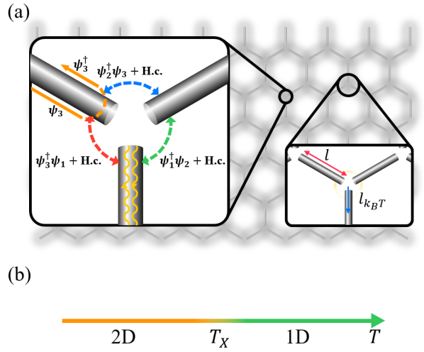
3. Dimensional Crossover: The energy scale can be translated to the lengthscale . Thus we can introduce the crossover temperature
| (4) |
which is the temperature where the thermal coherence length touches the wire length .[45] For , the electrons can ‘feel’ the finiteness of the wire length and recognize the network as the 2D system. The physics of this regime is essentially two-dimensional. On the other hand, above the crossover temperature, , we are probing the system at the lengthscale shorter than the segment length . Thus the system does not “know” that the wires form a 2D network, and the physics is largely governed by the properties of 1D wires and 0D junctions. Based on these observations, we can draw a “phase diagram” in [Fig.1(b)]. In real materials, we roughly estimate K in 1T-TaS2 and K in twisted bilayer graphenes (for nm, though it is tunable). For 1T-TiSe2, we estimate K with some assumptions. For the details and possible implications in existing experimental data, see [18].
We compare our crossover temperature Eq.(4) of the network with that of coupled wire systems or sliding LLs[46, 47, 48, 49, 50, 51, 52, 53, 54, 55, 56]. There, the wires are aligned along the same directions, and we assume only the short-ranged terms. Then the crossover temperature toward a regular 2D FL from the 1D TLL limit depends on both the intra- and interwire terms [46, 47, 48, 49, 50, 51, 52]
| (5) |
where is the strength of the interwire hopping, and is its scaling dimension.
In this Letter, we focus on the electric conduction in the network in the “1D TLL physics” regime
| (6) |
which has not been much explored. Since each segment is described by a scale-invariant TLL, the temperature dependence of the transport can be associated to the properties of the junctions. Hence, to study the network in this regime, we can utilize the RG analysis of junctions of TLLs [57, 45, 58, 59, 60]. Indeed, we find that the emergent NFLs in the network can be characterized by the RG fixed points of a single junction of TLLs. We will show that the RG fixed points of the junctions determine not only the leading dc conductivities but also leading scaling corrections, which are power-law in temperature . Namely, the NFL behavior is universal in the 1D regime (6) where the junction is described by a RG fixed point, which pins down the scaling dimensions of all the possible perturbations. Below we will explicitly illustrate this for the two simplest fixed points [60, 59], namely “disconnected fixed point” () and “connected fixed points”. As our terminology suggests, the connected fixed point gives rise the maximum conductances between the wires [60]. Some properties and stability of these fixed points are reviewed in [18].
4. Conduction through the Network: Here we show that the resistivity of the network is in general given by the power law (1) where the exponent is determined by the Luttinger parameter of the 1D TLL segment and the boundary conditions at the junctions. More precisely, where is the scaling dimension of the leading irrelevant operators at the junctions. The numerical coefficient depends on microscopic details. For example, for the disconnected fixed point, and
| (7) |
To establish this, we first show that the 0D electric conductance at a single junction determines the 2D conductivity of the whole network. For this, we imagine a perfect 2D network made out of the identical Y-junctions [Fig.1(a)]. We apply a uniform voltage drop across the -direction and then calculate the electric current flowing through the network [Fig.2]. In materials, electrons interact with the external environment such as phonons. In this Letter, as we consider the fairly high temperatures , we assume that the electron-phonon coherence length is shorter than the segment length . Then the electrons in the segment equilibrate, so that each segment has a well-defined voltage. Under this assumption, we can immediately compute the conductivity of the whole 2D network out of the “conductance tensor” of a single Y-junction.

Each fixed point of the Y-junction can be characterized by its conductance tensor , which relates the electric current at the -th wire with the voltage at the -th wire [Fig.2], i.e., . For the spinless fermions, all the known fixed points [60, 59] respect the permutation symmetry between the three neighboring wires. Hence the conductance tensor can be parameterized only by the two numbers and . Imposing at all the junctions, we can fix the electric current at every wires. From the current, we obtain the conductance of the entire network,[18] which is found to be proportional to the width, and inversely proportional to the length. (Similar discussions were given in [61, 62].) In this way, our network construction leads naturally to the classical Pouillet’s law, and the conduction property of the system can be characterized by constant conductivity tensors
| (8) |
The factors of and have the geometric origin, e.g., the size of the unitcell. We also checked and [18]. While the classical nature of the conduction is a natural consequence of the assumed local thermalization (and thus decoherence) in each segment, it is remarkable that the macroscopic property (conductivity) is determined by the property of the microscopic junctions, independently of the details of the thermalization. This can be regarded as a generalization of Landauer-Büttiker approach [63] to extensive macroscopic systems of interacting electrons.
Hence, we next compute and of an Y-junction at finite temperatures . For this, we generalize the results of [60, 59, 45, 57] to the Y-junctions. For instance, at the disconnected fixed point, the leading perturbation is the interwire hopping [Fig.1(a)]
where is identified with , and represents the electron annihilation operator of the -th wire at the Y-junction, i.e., . Up to the 2nd order in , we find [18]
| (9) |
with being the inverse of an UV cut-off of Eq.(2). The first term in is the universal conductance of the disconnected fixed point.[60, 59] The second term represents the correction from the leading irrelevant perturbation above. They are evaluated within the standard linear response theory combined with the perturbative expansion in [45, 57, 18]. The correction is consistent with Eq.(1), because the scaling dimension of is . As we have seen in Eq.(8), this conductance of the single junction directly gives the conductivity of the 2D network and the resistivity exponent is given as in Eq.(7). A fixed point is stable as far as the scaling dimension of the perturbation is larger than 1. Hence the disconnected fixed point is stable for . Furthermore, this disconnected fixed point is the only known stable fixed point for repulsive interactions[60, 59] and so this “strange insulator” behavior with the power-law divergence of the resistivity at low temperatures is generic.
For attractive interaction, , the inter-wire tunneling is a relevant perturbation. Eq.(9) could describe the conductivity at higher temperatures if the inter-wire coupling at the junction in the microscopic model is weak. In this case, the same expression (9) now describes the power-law with a positive resistivity exponent (7), namely the typical behavior of a metallic NFL. When the attractive interaction is sufficiently strong so that , as the temperature is lowered, the junction is governed by the connected fixed point. This fixed point is stable for because the scaling dimension of the leading irrelevant operators at this fixed point is [60, 18]. Taking the operators into account, we can again evaluate the conductance within the standard linear response theory[45, 57, 18]
| (10) |
where we suppressed all the unimportant constants into . As before, the first term is the universal conductance of the connected fixed point,[60, 59] and the second term is the correction from the perturbative expansion of the leading irrelevant operators.[18] If the inter-wire coupling at the junction is strong, Eq.(10) would describe the entire temperature range where the 1D TLL description is valid. This also gives the metallic NFL behavior with the decreasing resistivity at lower temperatures, but with the resistivity exponent .
For both the disconnected and connected fixed points, and thus the Hall conductivity vanish, as expected from the time-reversal invariance of the underlying model. On the other hand, for the network of under a uniform magnetic field, the chiral fixed point of is stabilized:
| (11) |
up to the perturbative correction . Such network is metallic and has the “universal” Hall conductivity, which is determined by the Luttinger parameter [38, 18]. This result is consistent with [38], which considered the electric conduction across a network consist of the chiral fixed point. We note that however, [38] missed much of the NFL physics which we explored here. See the comparison in [18]. While the realization of the chiral fixed point requires an explicit breaking of the time-reversal invariance, in principle the required breaking can be infinitesimal, e.g., by a very weak magnetic field through the junctions [59, 60]. This behavior is again quite different from a normal metal, in which the Hall conductivity is proportional to the applied magnetic field. We also note that for or , the chiral fixed point is unstable. Instead, the connected and disconnected fixed points are stable as discussed above.
Let us give a few remarks on Eqs.(9), (10), and (11), which represent the conductance in the vicinity of three different RG fixed points for the junction. First of all, in all cases, the conductivity of the network exhibits a power law in temperature, whose exponent continuously evolves as the Luttinger parameter varies. This is the manifestation of the exact marginality of the Luttinger parameter. Essentially, this marginality allows the scaling dimension of electrons vary smoothly, which translates as the continuously changing in Eq.(7). In experiment, this means that, as the external parameters, e.g., pressure and gating, are tuned, the exponent of the temperature dependence of the resistivity will continuously change. This is markedly different from the behavior of a regular Fermi Liquid, where the exactly marginal deformation, i.e., the change of the Fermi velocity, does not alter the temperature dependence of the transport coefficients.
Finally, we comment on possible effects of disorders on transport. There are distinct types of the disorders at different length scales. For instance, microscopic impurities in TLLs will induce a power-law correction to the conductivity,[45, 57, 64] which will add up to those from the junctions. Similarly, randomly missing (completely disconnected) Y-junctions will introduce an additional correction. Details are given in [18].
5. Conclusions: We have demonstrated the emergence of a novel class NFLs in the conducting networks, whose universal properties are controlled by the RG fixed points of the junction of TLLs. This makes our network system a unique theoretical platform, where the isotropic NFL behaviors in dimensions can be deduced from the well-established theory on strongly correlated electrons in 1D. The NFLs we have proposed are potentially already out there[10, 19, 17, 24, 18] in experiments, and/or can be easily realized and verified in currently-available setups. For instance, one can artificially pattern the network superstructure in experiments[65]. In twisted bilayer graphenes, the crossover temperature , which is related with the length of the underlying wires, can be controlled by tuning the twisting angle. Hence, in these systems one can look at the dependence of the conductivities on temperature and twisting angles to observe the emergence of the putative NFLs, which will be quite spectacular!
Once the power-law behavior of the resistivity is observed, the Luttinger parameter for the TLL describing each segment is inferred from the resistivity exponent . Our scenario can then be verified by a consistency check with an independent determination of the Luttinger parameter of the 1D segment, for example by ARPES measurement of the local density of states [66]. The Luttinger parameter and scaling dimensions of the leading irrelevant operators at the junctions can be also extracted from the specific heat and susceptibility . For example, the specific heat has the two contributions, one from the 1D TLLs and the other from the junctions.[67, 68, 69] The 1D part scales as , but the junction contribution has .[67, 68, 69] Hence in total and similarly . In the future, it will be interesting to investigate explicitly the effect of the long-range Coulomb interaction on the network NFLs, following the related studies on a single TLL and coupled wires [70, 71, 72, 73, 74, 75, 76].
Acknowledgements.
We thank Chenhua Geng, Jung Hoon Han, Jun-Sung Kim, Gil-Ho Lee, Sung-Sik Lee, Jeffrey Teo and Han Woong Yeom for helpful discussion. JL and GYC are supported by the National Research Foundation of Korea (NRF) grant funded by the Korea government(MSIT) (No. 2020R1C1C1006048 and No.2020R1A4A3079707) and also by IBS-R014-D1. This work is supported by the Air Force Office of Scientific Research under award number FA2386-20-1-4029. MO is supported in part by MEXT/JSPS KAKENHI Grants No. JP18H03686 and No. JP17H06462, and JST CREST Grant No. JPMJCR19T2. We also thank Claudio Chamon and Dmitry Green for bringing our attention to the reference [38] and helpful discussions.References
- Nozieres and Pines [1999] P. Nozieres and D. Pines, Theory Of Quantum Liquids, Advanced Books Classics (Avalon Publishing, 1999), ISBN 9780813346533.
- Lee [2018] S.-S. Lee, Annual Review of Condensed Matter Physics 9, 227 (2018).
- Schofield [1999] A. J. Schofield, Contemporary Physics 40, 95 (1999).
- Varma et al. [2002] C. Varma, Z. Nussinov, and W. van Saarloos, Physics Reports 361, 267 (2002).
- Donos and Hartnoll [2013] A. Donos and S. A. Hartnoll, Nature Physics 9, 649 (2013).
- Donos and Gauntlett [2014] A. Donos and J. P. Gauntlett, Journal of High Energy Physics 2014, 7 (2014).
- Andrade and Krikun [2019] T. Andrade and A. Krikun, Journal of High Energy Physics 2019, 119 (2019).
- Rickhaus et al. [2018] P. Rickhaus, J. Wallbank, S. Slizovskiy, R. Pisoni, H. Overweg, Y. Lee, M. Eich, M.-H. Liu, K. Watanabe, T. Taniguchi, et al., Nano letters 18, 6725 (2018).
- Yoo et al. [2019] H. Yoo, R. Engelke, S. Carr, S. Fang, K. Zhang, P. Cazeaux, S. H. Sung, R. Hovden, A. W. Tsen, T. Taniguchi, et al., Nature materials 18, 448 (2019).
- Xu et al. [2019] S. Xu, A. Berdyugin, P. Kumaravadivel, F. Guinea, R. K. Kumar, D. Bandurin, S. Morozov, W. Kuang, B. Tsim, S. Liu, et al., Nature communications 10, 1 (2019).
- Ma et al. [2017a] Y. Ma, S. Kolekar, H. Coy Diaz, J. Aprojanz, I. Miccoli, C. Tegenkamp, and M. Batzill, ACS nano 11, 5130 (2017a).
- Carr et al. [2018] S. Carr, D. Massatt, S. B. Torrisi, P. Cazeaux, M. Luskin, and E. Kaxiras, Physical Review B 98, 224102 (2018).
- Weston et al. [2020] A. Weston, Y. Zou, V. Enaldiev, A. Summerfield, N. Clark, V. Zólyomi, A. Graham, C. Yelgel, S. Magorrian, M. Zhou, et al., Nature Nanotechnology pp. 1–6 (2020).
- Morishita [2019] M. Morishita, pp. 1–5 (2019), eprint 1908.01991, URL http://arxiv.org/abs/1908.01991.
- Park et al. [2019] J. W. Park, G. Y. Cho, J. Lee, and H. W. Yeom, Nature Communications 10, 1 (2019), URL http://dx.doi.org/10.1038/s41467-019-11981-5.
- Spijkerman et al. [1997] A. Spijkerman, J. L. de Boer, A. Meetsma, G. A. Wiegers, and S. van Smaalen, Phys. Rev. B 56, 13757 (1997), URL https://link.aps.org/doi/10.1103/PhysRevB.56.13757.
- Li et al. [2016] L. Li, E. O’farrell, K. Loh, G. Eda, B. Özyilmaz, and A. C. Neto, Nature 529, 185 (2016).
- [18] See the supplemental material for details, which includes Refs. [15, 19, 10, 17, 22, 77, 78, 24, 79, 80, 81, 82, 83, 84, 85, 86, 38, 60, 57, 87].
- Sipos et al. [2008] B. Sipos, A. F. Kusmartseva, A. Akrap, H. Berger, L. Forró, and E. Tutiš, Nature materials 7, 960 (2008).
- Yu et al. [2015] Y. Yu, F. Yang, X. F. Lu, Y. J. Yan, Y.-H. Cho, L. Ma, X. Niu, S. Kim, Y.-W. Son, D. Feng, et al., Nature nanotechnology 10, 270 (2015).
- Liu et al. [2016] Y. Liu, D. F. Shao, L. J. Li, W. J. Lu, X. D. Zhu, P. Tong, R. C. Xiao, L. S. Ling, C. Y. Xi, L. Pi, et al., Phys. Rev. B 94, 045131 (2016), URL https://link.aps.org/doi/10.1103/PhysRevB.94.045131.
- Chen et al. [2019] C. Chen, L. Su, A. C. Neto, and V. M. Pereira, Physical Review B 99, 121108 (2019).
- Wang et al. [2019] L. Wang, E.-M. Shih, A. Ghiotto, L. Xian, D. A. Rhodes, C. Tan, M. Claassen, D. M. Kennes, Y. Bai, B. Kim, et al., arXiv preprint arXiv:1910.12147 (2019).
- Kusmartseva et al. [2009] A. F. Kusmartseva, B. Sipos, H. Berger, L. Forro, and E. Tutiš, Physical review letters 103, 236401 (2009).
- Fazekas and Tosatti [1980] P. Fazekas and E. Tosatti, Physica B+ C 99, 183 (1980).
- Lee et al. [2020] J. M. Lee, C. Geng, J. W. Park, M. Oshikawa, S.-S. Lee, H. W. Yeom, and G. Y. Cho, Physical Review Letters 124, 137002 (2020).
- Mizoguchi et al. [2019] T. Mizoguchi, M. Maruyama, S. Okada, and Y. Hatsugai, Phys. Rev. Materials 3, 114201 (2019), URL https://link.aps.org/doi/10.1103/PhysRevMaterials.3.114201.
- Wu et al. [2019] X.-C. Wu, C.-M. Jian, and C. Xu, Physical Review B 99, 161405 (2019).
- Chou et al. [2019] Y.-Z. Chou, Y.-P. Lin, S. Das Sarma, and R. M. Nandkishore, Phys. Rev. B 100, 115128 (2019), URL https://link.aps.org/doi/10.1103/PhysRevB.100.115128.
- Cao et al. [2018a] Y. Cao, V. Fatemi, A. Demir, S. Fang, S. L. Tomarken, J. Y. Luo, J. D. Sanchez-Yamagishi, K. Watanabe, T. Taniguchi, E. Kaxiras, et al., Nature 556, 80 (2018a).
- Cao et al. [2018b] Y. Cao, V. Fatemi, S. Fang, K. Watanabe, T. Taniguchi, E. Kaxiras, and P. Jarillo-Herrero, Nature 556, 43 (2018b).
- Efimkin and MacDonald [2018] D. K. Efimkin and A. H. MacDonald, Physical Review B 98, 035404 (2018).
- Chalker and Coddington [1988] J. Chalker and P. Coddington, Journal of Physics C: Solid State Physics 21, 2665 (1988).
- Chou et al. [2020] Y.-Z. Chou, F. Wu, and S. D. Sarma, Hofstadter butterfly and floquet topological insulators in minimally twisted bilayer graphene (2020), eprint 2004.15022.
- De Beule et al. [2020] C. De Beule, F. Dominguez, and P. Recher, Phys. Rev. Lett. 125, 096402 (2020), URL https://link.aps.org/doi/10.1103/PhysRevLett.125.096402.
- Ferraz et al. [2019] G. Ferraz, F. B. Ramos, R. Egger, and R. G. Pereira, Phys. Rev. Lett. 123, 137202 (2019), URL https://link.aps.org/doi/10.1103/PhysRevLett.123.137202.
- Chen et al. [2020] C. Chen, A. H. Castro Neto, and V. M. Pereira, Phys. Rev. B 101, 165431 (2020), URL https://link.aps.org/doi/10.1103/PhysRevB.101.165431.
- Medina et al. [2013] J. Medina, D. Green, and C. Chamon, Physical Review B 87, 045128 (2013).
- Bockrath et al. [1999] M. Bockrath, D. H. Cobden, J. Lu, A. G. Rinzler, R. E. Smalley, L. Balents, and P. L. McEuen, Nature 397, 598 (1999).
- Ma et al. [2017b] Y. Ma, H. C. Diaz, J. Avila, C. Chen, V. Kalappattil, R. Das, M.-H. Phan, T. Čadež, J. M. P. Carmelo, M. C. Asensio, et al., Nature Communications 8, 14231 (2017b), URL http://www.nature.com/articles/ncomms14231.
- Kim et al. [2007] N. Y. Kim, P. Recher, W. D. Oliver, Y. Yamamoto, J. Kong, and H. Dai, Physical Review Letters 99, 036802 (2007), URL https://link.aps.org/doi/10.1103/PhysRevLett.99.036802.
- Zhen et al. [1999] Y. Zhen, H. W. Postma, L. Balents, and C. Dekker, Nature 402, 273 (1999).
- Zhao et al. [2018] S. Zhao, S. Wang, F. Wu, W. Shi, I. B. Utama, T. Lyu, L. Jiang, Y. Su, S. Wang, K. Watanabe, et al., Physical Review Letters 121 (2018).
- Kim et al. [2020] M. Kim, S. G. Xu, A. I. Berdyugin, A. Principi, S. Slizovskiy, N. Xin, P. Kumaravadivel, W. Kuang, M. Hamer, R. Krishna Kumar, et al., Nature Communications 11, 2339 (2020), URL http://www.nature.com/articles/s41467-020-15829-1.
- Kane and Fisher [1992a] C. Kane and M. P. Fisher, Physical Review B 46, 15233 (1992a).
- Wen [1990] X. G. Wen, Physical Review B 42, 6623 (1990), URL https://link.aps.org/doi/10.1103/PhysRevB.42.6623.
- SCHULZ [1991] H. SCHULZ, International Journal of Modern Physics B 05, 57 (1991), URL https://www.worldscientific.com/doi/abs/10.1142/S0217979291000055.
- Cas [1992] Physical Review Letters 69, 1703 (1992), URL https://link.aps.org/doi/10.1103/PhysRevLett.69.1703.
- Brazovskii and Yakovenko [1985] S. Brazovskii and V. Yakovenko, Zh. Eksp. Teor. Fiz 89, 2318 (1985).
- Bourbonnais and Caron [1986] C. Bourbonnais and L. Caron, Physica B+C 143, 450 (1986), URL https://linkinghub.elsevier.com/retrieve/pii/0378436386901646.
- Giamarchi [2003] T. Giamarchi, Quantum physics in one dimension, vol. 121 (Clarendon press, 2003).
- Guinea and Zimanyi [1993] F. Guinea and G. Zimanyi, Physical Review B 47, 501 (1993), URL https://link.aps.org/doi/10.1103/PhysRevB.47.501.
- Sondhi and Yang [2001] S. L. Sondhi and K. Yang, Physical Review B 63, 054430 (2001), URL https://link.aps.org/doi/10.1103/PhysRevB.63.054430.
- Mukhopadhyay et al. [2001] R. Mukhopadhyay, C. L. Kane, and T. C. Lubensky, Physical Review B 64, 045120 (2001), URL https://link.aps.org/doi/10.1103/PhysRevB.64.045120.
- Emery et al. [2000] V. J. Emery, E. Fradkin, S. A. Kivelson, and T. C. Lubensky, Physical Review Letters 85, 2160 (2000), URL https://link.aps.org/doi/10.1103/PhysRevLett.85.2160.
- Vishwanath and Carpentier [2001] A. Vishwanath and D. Carpentier, Physical Review Letters 86, 676 (2001), URL https://link.aps.org/doi/10.1103/PhysRevLett.86.676.
- Kane and Fisher [1992b] C. Kane and M. P. Fisher, Physical review letters 68, 1220 (1992b).
- Furusaki and Nagaosa [1993] A. Furusaki and N. Nagaosa, Phys. Rev. B 47, 4631 (1993), URL https://link.aps.org/doi/10.1103/PhysRevB.47.4631.
- Chamon et al. [2003] C. Chamon, M. Oshikawa, and I. Affleck, Physical review letters 91, 206403 (2003).
- Oshikawa et al. [2006] M. Oshikawa, C. Chamon, and I. Affleck, Journal of Statistical Mechanics: Theory and Experiment 2006, P02008 (2006).
- d’Amato and Pastawski [1990] J. L. d’Amato and H. M. Pastawski, Physical Review B 41, 7411 (1990).
- Büttiker [1986] M. Büttiker, Phys. Rev. B 33, 3020 (1986), URL https://link.aps.org/doi/10.1103/PhysRevB.33.3020.
- Datta [1997] S. Datta, Electronic transport in mesoscopic systems (Cambridge university press, 1997).
- Giamarchi and Maurey [1996] T. Giamarchi and H. Maurey (1996), eprint 9608006, URL http://arxiv.org/abs/cond-mat/9608006.
- Forsythe et al. [2018] C. Forsythe, X. Zhou, K. Watanabe, T. Taniguchi, A. Pasupathy, P. Moon, M. Koshino, P. Kim, and C. R. Dean, Nature nanotechnology 13, 566 (2018).
- Ishii et al. [2003] H. Ishii, H. Kataura, H. Shiozawa, H. Yoshioka, H. Otsubo, Y. Takayama, T. Miyahara, S. Suzuki, Y. Achiba, M. Nakatake, et al., Nature 426, 540 (2003).
- Fujimoto [2003] S. Fujimoto (2003), eprint 0308046, URL http://arxiv.org/abs/cond-mat/0308046.
- Fujimoto and Eggert [2004] S. Fujimoto and S. Eggert, Physical Review Letters 92, 037206 (2004), URL https://link.aps.org/doi/10.1103/PhysRevLett.92.037206.
- Furusaki and Hikihara [2004] A. Furusaki and T. Hikihara, Physical Review B 69, 094429 (2004), URL https://link.aps.org/doi/10.1103/PhysRevB.69.094429.
- Kane et al. [1997] C. Kane, L. Balents, and M. P. Fisher, Physical Review Letters 79, 5086 (1997).
- Wang et al. [2001] D. W. Wang, S. Das Sarma, and A. J. Millis, Physical Review B - Condensed Matter and Materials Physics 64, 193307 (2001), URL https://link.aps.org/doi/10.1103/PhysRevB.64.193307.
- Vu et al. [2020] D. Vu, A. Iucci, and S. Das Sarma, Physical Review Research 2, 023246 (2020), URL https://link.aps.org/doi/10.1103/PhysRevResearch.2.023246.
- Schulz [1993] H. J. Schulz, Physical Review Letters 71, 1864 (1993), URL https://link.aps.org/doi/10.1103/PhysRevLett.71.1864.
- Sur and Yang [2017] S. Sur and K. Yang, Physical Review B 96, 075131 (2017), URL https://link.aps.org/doi/10.1103/PhysRevB.96.075131.
- Kopietz et al. [1995] P. Kopietz, V. Meden, and K. Schönhammer, Physical Review Letters 74, 2997 (1995), URL https://link.aps.org/doi/10.1103/PhysRevLett.74.2997.
- Kopietz et al. [1997] P. Kopietz, V. Meden, and K. Schönhammer, Physical Review B 56, 7232 (1997), URL https://link.aps.org/doi/10.1103/PhysRevB.56.7232.
- Qian et al. [2007] D. Qian, D. Hsieh, L. Wray, E. Morosan, N. Wang, Y. Xia, R. Cava, and M. Hasan, Physical review letters 98, 117007 (2007).
- Yan et al. [2017] S. Yan, D. Iaia, E. Morosan, E. Fradkin, P. Abbamonte, and V. Madhavan, Phys. Rev. Lett. 118, 106405 (2017), URL https://link.aps.org/doi/10.1103/PhysRevLett.118.106405.
- Paredes et al. [2004] B. Paredes, A. Widera, V. Murg, O. Mandel, S. Fölling, I. Cirac, G. V. Shlyapnikov, T. W. Hänsch, and I. Bloch, Nature 429, 277 (2004), URL http://www.nature.com/articles/nature02530.
- Haller et al. [2010] E. Haller, R. Hart, M. J. Mark, J. G. Danzl, L. Reichsöllner, M. Gustavsson, M. Dalmonte, G. Pupillo, and H. C. Nägerl, Nature 466, 597 (2010).
- Angelakis et al. [2011] D. G. Angelakis, M. Huo, E. Kyoseva, and L. C. Kwek, Physical Review Letters 106, 1 (2011).
- Kwon et al. [2020] W. J. Kwon, G. Del Pace, R. Panza, M. Inguscio, W. Zwerger, M. Zaccanti, F. Scazza, and G. Roati, Science 369, 84 (2020), URL https://www.sciencemag.org/lookup/doi/10.1126/science.aaz2463.
- Fukuhara et al. [2013] T. Fukuhara, A. Kantian, M. Endres, M. Cheneau, P. Schauß, S. Hild, D. Bellem, U. Schollwöck, T. Giamarchi, C. Gross, et al., Nature Physics 9, 235 (2013), URL http://www.nature.com/articles/nphys2561.
- Häusler et al. [2017] S. Häusler, S. Nakajima, M. Lebrat, D. Husmann, S. Krinner, T. Esslinger, and J.-P. Brantut, Physical Review Letters 119, 030403 (2017), URL http://link.aps.org/doi/10.1103/PhysRevLett.119.030403.
- Mazurenko et al. [2017] A. Mazurenko, C. S. Chiu, G. Ji, M. F. Parsons, M. Kanász-Nagy, R. Schmidt, F. Grusdt, E. Demler, D. Greif, and M. Greiner, Nature 545, 462 (2017).
- Schäfer et al. [2020] F. Schäfer, T. Fukuhara, S. Sugawa, Y. Takasu, and Y. Takahashi, Nature Reviews Physics 2, 411 (2020).
- Nayak et al. [1999] C. Nayak, M. P. A. Fisher, A. W. W. Ludwig, and H. H. Lin, Physical Review B 59, 15694 (1999), URL https://link.aps.org/doi/10.1103/PhysRevB.59.15694.