Quantum Coulomb glass on the Bethe lattice

Abstract

We study the Coulomb glass emerging from the interplay of strong interactions and disorder in a model of spinless fermions on the Bethe lattice. In the infinite coordination number limit, strong interactions induce a metallic Coulomb glass phase with a pseudogap structure at the Fermi energy. Quantum and thermal fluctuations both melt this glass and induce a disordered quantum liquid phase. We combine self-consistent diagrammatic perturbation theory with continuous time quantum Monte-Carlo simulations to obtain the complete phase diagram of the electron glass, and to characterize its dynamical properties in the quantum liquid, as well as in the replica symmetry broken glassy phase. Tunneling spectra display an Efros-Shklovskii pseudogap upon decreasing temperatures, but the density of states remains finite at the Fermi energy due to residual quantum fluctuations. Our results bear relevance to the metallic glass phase observed in Si inversion layers.

I Introduction

Describing the localization of disordered electrons in the presence of long-ranged Coulomb interactions and the melting of the Coulomb glass due to quantum-fluctuations represent some of the most challenging unsolved and elusive problems in modern condensed matter physics [1]. In the absence of interactions, disorder tends to suppress quantum fluctuations, and leads to Anderson localization [2, 3].

The presence of interactions, however, changes the structure of localization transition entirely: unscreened Coulomb interactions lead to stronger and stronger anomalies on the metallic side as one approaches the phase transition [4], amount in the formation of curious spin fluctuations [5], and lead to the emergence of the Coulomb gap [6, 7] on the insulating side, accompanied by glassy dynamics and memory effects [8, 9, 10, 11]. A major step towards understanding this quantum phase transition has been made by A. M. Finkel’stein, who developed a scaling theory in the presence of Coulomb interactions and weak disorder [12]. Certain implications of this scaling theory regarding the critical behavior have been verified experimentally [13], but a perturbative scaling theory leaves the structure of the localized phase unrevealed, and has little to say about properties of the localized phase such as the formation of the pseudogap or the glassy structure of the localized phase, not to mention the connection with many-body localization [14, 15].

The influence of quantum tunneling on the Coulomb gap has been addressed initially by means of numerical approaches. A configuration interaction approximation based computation predicted a considerable reduction of the width of the Coulomb gap [16], while Hartree-Fock calculations predicted a modification of the structure of the classical Efros-Shklovskii pseudogapclose to the Fermi surface [17, 18].

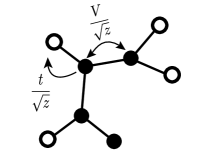
Figure 1: Sketch of the mean field electron glass model, Eq. (1). Electrons move on a disordered Bethe lattice of coordination number $z$, can hop between neighboring sites, and interact through a Coulomb interaction with nearest neighbors.

A major step towards understanding the quantum melting of the Coulomb glass is the construction of a solvable mean field theory, similar to the Sherrington-Kirkpatrick (SK) model, the standard mean field model of classical and quantum spin glass transitions [19, 20, 21, 22]. Such a mean field model, accounting for most essential properties of the Coulomb glass phase except Anderson localization, has been proposed by Pastor and Dobrosavljević in their seminal work [23], possibly inspired by the extended dynamical mean field approach applied to clean correlated systems [24, 25, 26]. In the spinless version of their model, electrons move on a Bethe lattice of coordination $z\to\infty$, experience some onsite disorder, $\varepsilon_{i}$, and interact with each other through a repulsive nearest neighbor interaction, $V_{ij}=V/\sqrt{z}$, mimicking the long-ranged Coulomb interaction (see Fig. 1),

$$\hat{H}=-\dfrac{t}{\sqrt{z}}\sum_{\langle i,j\rangle}\left(\hat{c}^{\dagger}_{i}\hat{c}_{j}+{\rm h.c}\right)+\dfrac{V}{\sqrt{z}}\delta\hat{n}_{i}\delta\hat{n}_{j}+\sum_{i}\varepsilon_{i}\delta\hat{n}_{i}\;.$$ (1)

Here $\delta\hat{n}_{i}=\hat{c}_{i}^{\dagger}\hat{c}_{i}-1/2$ denotes deviations from half-filling, and the levels $\varepsilon_{i}$ are drawn from a Gaussian distribution, $P(\varepsilon)\sim e^{-\varepsilon^{2}/(2W^{2})}$. In the rest of the paper, we shall refer to this model as the disordered $t-V$ model.

As shown in Ref. [23], even though the interaction is uniform, spontaneous density fluctuations lead to the emergence of a glass phase, and the model (1) maps onto the Sherrington-Kirkpatrick model in the absence of quantum tunneling, $t=0$. We emphasize that this transition is structural in the sense that it takes place even in the absence of disorder, $W\to 0$, and is driven by interactions rather than disorder. Here, in contrast to the SK model, frustrations do not originate from a frustrated interaction: rather, a fluctuation in the occupation of some levels creates a ”frustration by choice”, leading to the glass transition.

Later works revealed a number of key properties of the disordered $t-V$ model, Eq. (1). The quantum critical behavior has been analyzed for small disorder in terms of a Landau theory [27, 28], following a line similar to the work of Read, Sachdev, and Ye [29], and it has been argued that for finite coordination numbers, $z$, a glassy metallic phase should separate the glassy insulating phase from the disordered Fermi liquid [30], as observed on low mobility Si inversion layers [31].

Nevertheless, in spite of all these achievements and efforts, a complete solution of (1) is still missing, even in the mean field limit, $z\to\infty$. Here we attempt to give such an accurate and extensive numerical solution of the disordered $t-V$ model in the $z\to\infty$, mean field limit. In addition to determining the complete phase diagram, the distribution of local levels, the order parameter, the free energy, and the entropy, we also determine the spectral properties and the tunneling spectra of the electrons, as well as their scaling properties away from the critical point.

The solution of (1) represents a quite challenging task: to enter the glassy phase and capture the formation of the pseudogap, we must allow for complete replica symmetry breaking, –– accounting for the distribution of local (renormalized) energy levels, –- and, at the same time, we must solve an ensemble of quantum impurity problems coupled self-consistently back to the spin glass order parameter [32, 33, 34]. This route has been followed in Ref. [35] to study the glassy phase of the – somewhat simpler – transverse field Sherrington-Kirkpatrick model. Here we derive the appropriate equations for the mean field Coulomb glass model by using a path integral formalism, and solve the mean field theory numerically.

We apply two different numerical methods: In the Fermi liquid phase, we use an extended continuous time Quantum Monte-Carlo (CTQMC) dynamical mean field approach. This method provides us the numerically exact, self-consistent solution, however, is numerically demanding, and is only appropriate to give us a solution at a relatively small number of points in parameter space. We therefore combine this approach with an Iterative Perturbation Theory (IPT), similar in spirit to the one used to describe the Mott transition in a pioneering work by A. Georges et al. [36]. A combination of these two approaches allows us to obtain a coherent picture, summarized in Fig. 2.

For convenience, we measure all energy scales in Fig. 2 in the disorder strength, $W$. Phase boundaries in Fig. 2.a correspond to replica symmetry breaking. The electron glass forms at large interactions, and is destroyed both by thermal ($\sim T$) and by quantum ($\sim t$) fluctuations. Typical spectral densities are presented in Fig. 2(b) at a transition point, where $T\ll t$, and therefore quantum fluctuations drive the quantum glass to quantum liquid phase transition. A marked correlation hole structure starts to form already at the critical point. This anomaly gradually develops into a pseudogap that gets deeper and deeper as we enter the glass phase, but the density of states remains finite at the Fermi energy in the glass phase for any finite quantum tunneling, even in the $T=0$ temperature limit. This is a peculiarity of the exactly solvable mean field limit $z=\infty$, where no Anderson localization takes place. The glass state we find is therefore identified as a metallic (spinless) electron glass, observed in several experiments [31, 37, 38]. A similar glassy metallic phase has been predicted to emerge in itinerant fermionic systems with cavity mediated long-range interactions, based on a replica symmetric effective field theory approach [39].

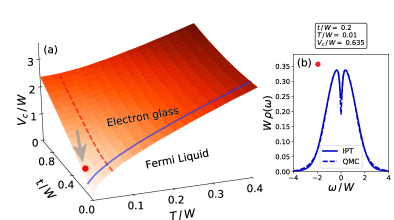
Figure 2: (a) Boundary separating the Fermi liquid and the electron glass phases. Cuts along the solid and dashed lines are presented in Fig. 6. (b) Spectral function computed at the quantum phase transition point, indicated in panel (a) by the arrow. A correlation hole preceding the pseudogap structure starts to form already at the phase boundary.

The rest of the paper is organized as follows. In Sec. II, we introduce the mean field equations through an intuitive cavity approach as well as the more technical replica method, and then formulate the resulting self-consistency equations for the replica symmetric solution and for full replica symmetry breaking. Sec. III is devoted to the more technical aspects of the solution. There we discuss the faster but approximate iterative perturbation theory (Sec.  III.1) and the exact but numerically more demanding continuous time quantum Monte Carlo (CTQMC) method (Sec.  III.2). In the rest of the paper we present our results. The spectral function in the replica symmetric Fermi liquid phase as well as the phase boundary of the electron glass phase are presented in Sec. IV. Sec. V is devoted to the glassy phase: we discuss there the evolution of the order parameter, the distribution of Hartree energies, and the properties of the spectral function deep in the glassy phase. We discuss the thermodynamics of the mean field Coulomb glass model in Sec. VI. Our main findings are summarized in Sec. VII. Technical details on the CTQMC simulations and on the numerical solution in the replica symmetry broken phase are relegated to appendices.

II Mean field equations

The mean field equations of disordered $t-V$ model (1) have been derived for $z\to\infty$ using the replica method in Ref. [23]. To our knowledge, these equations have, however, never been solved before in their full power. In fact, to obtain a full solution and to capture the formation of the Coulomb gap, one must consider the structure of full replica symmetry breaking, just as for the Sherrington-Kirckpatrick model [40, 41, 42, 34].

Before we discuss the quite technical replica method, let us start with a cavity consideration. This allows one to understand the ultimate structure of the equations to be solved.

II.1 Cavity approach and effective local action

Let us focus on site $i=0$, and write the action corresponding to the Hamiltonian (1) as follows:

$$S =\int_{\tau}{\overline{c}}_{0\,\tau}(\partial_{\tau}+\epsilon_{0})c_{0\,\tau}+\frac{V}{\sqrt{z}}{\sum_{i}}^{\prime}\int_{\tau}\delta n_{0,\tau}\delta n_{i,\tau}-\frac{t}{\sqrt{z}}{\sum_{i}}^{\prime}\int_{\tau}({\overline{c}}_{0\,\tau}{c}_{i\,\tau}+h.c.)+S_{i\neq 0}\;.$$ (2)

Here we used the shorthand notation, $\int_{\tau}=\int_{0}^{\beta}{\rm{d}\tau}$, with $\beta$ the inverse temperature, and have separated those pieces, which involve site $0$. Primes indicate summations over nearest neighbors only. We can then formally expand $e^{-S}$, and integrate out all $i\neq 0$ sites to obtain an effective action for site 0,

$$S_{0}^{\rm eff} =\int_{\tau}\overline{c}_{0\,\tau}(\partial_{\tau}+\epsilon_{0}){c}_{0\,\tau}-t^{2}\int_{\tau}\int_{\tau^{\prime}}{\overline{c}}_{0\,\tau}{c}_{0\,\tau^{\prime}}\;\frac{1}{z}{\sum_{i}}^{\prime}\langle c_{i\,\tau}{\overline{c}}_{i\,\tau^{\prime}}\rangle_{\rm cav}+\frac{V}{\sqrt{z}}{\sum_{i}}^{\prime}\int_{\tau}\delta n_{0,\tau}\langle\delta n_{i,\tau}\rangle_{\rm cav}$$

$$-\frac{V^{2}}{2}\int_{\tau}\int_{\tau^{\prime}}\delta n_{0,\tau}\delta n_{0,\tau^{\prime}}\frac{1}{z}{\sum_{i}}^{\prime}\langle\delta n_{i,\tau}\delta n_{i,\tau^{\prime}}\rangle_{\rm cav}\;+\dots.$$ (3)

Here the $\langle\ldots\rangle_{\rm cav}$ denote cavity averages, i.e. averages computed in the absence of site $i=0$. Higher order contributions, that are not displayed, vanish in the $z\to\infty$ limit on the Bethe lattice. The third term in this expansion represents a random chemical potential, arising from charge fluctuations at neighboring sites. We can rewrite the above action as

$$S_{0}^{\rm eff}= \int_{\tau}\int_{\tau^{\prime}}\Big{\{}\overline{c}_{0\,\tau}\big{(}\delta(\tau-\tau^{\prime})(\partial_{\tau}+{\tilde{\epsilon}}_{0})-t^{2}G(\tau-\tau^{\prime})\big{)}{c}_{0\,\tau^{\prime}}\;-\frac{V^{2}}{2}\chi(\tau-\tau^{\prime})\delta n_{0,\tau}\delta n_{0,\tau^{\prime}}\Big{\}}\;,$$ (4)

with $G$ and $\chi$ denoting a nearest neighbour average over cavity Green’s functions and dynamical susceptibilities, and the random field ${\tilde{\epsilon}}_{0}$ incorporating charge fluctuations on neighbouring sites into the bare local field, $\epsilon_{0}$. Since the presence of site 0 induces a perturbation of order $\sim 1/\sqrt{z}$ on its nearest neighbors, $G$ and $\chi$ can be replaced by the lattice average of the local Green’s function and dynamical charge susceptibility, respectively. Would we know the distribution of ${\tilde{\epsilon}}_{0}$, $\widetilde{P}(\tilde{\epsilon})$, we could replace these spacial averages by an average over $\tilde{\epsilon}$. We could thus solve the action (4) for $G_{\tilde{\epsilon}}(\tau)$ and $\chi_{\tilde{\epsilon}}(\tau)$, and obtain $G(\tau)$ and $\chi(\tau)$ by averaging over $P(\tilde{\epsilon})$, thereby closing a dynamical mean field theory (DMFT) cycle.

Unfortunately, it is not so simple to obtain $\widetilde{P}(\tilde{\epsilon})$. The difficulty is related to spontaneous symmetry breaking. Even for a given set of the on site energies, $\{\epsilon_{i}\}$, each ’leg’ attached to the cavity has namely many symmetry broken states. We should pick a symmetry broken charge distribution on each of these legs. However, we cannot choose these independently of each other, since the central site $i=0$ creates correlations between the legs. Adding/removing the site 0 induces namely a correlated charge shift of order $\sim 1/\sqrt{z}$ on neighboring charge distributions. This, in turn, amounts in a change of ${\cal O}(1)$ in the value of $\tilde{\epsilon}_{0}$ and, more importantly, correlates the occupation of neighboring sites through charge fluctuations at site $i=0$. The situation is quite similar to that of the ferromagnetic phase of an Ising magnet on the Bethe lattice, where the direction of magnetization on each leg gets correlated through the central site.

The appropriate distribution $\widetilde{P}(\tilde{\epsilon})$ follows from stability criteria, usually formulated in terms of the replica method, discussed in the next subsection. We shall also follow this – somewhat formal – route to determine $\widetilde{P}(\tilde{\epsilon})$.

II.2 Replica approach

The action $S_{0}^{\rm eff}$ in Eq. (4) can also be obtained via the replica trick, whereby we express the logarithm of the partition function as

$$\log Z=\lim_{n\rightarrow 0}\dfrac{Z^{n}-1}{n}\;.$$ (5)

We therefore take $n\to 0$ copies of the Hamiltonian, integrate out the Gaussian disorder and the fermions at all sites excepting the central one. The latter step becomes simple in the $z\to\infty$ limit, where a systematic $1/z$ cumulant expansion leads to a simple (extended) dynamical mean field theory structure [43] with the effective action 

$$S_{\rm rep}=\int_{0}^{\beta}d\tau\int_{0}^{\beta}d\tau^{\prime} \Bigg{\{}\sum_{a=0}^{n}\left(\overline{c}_{\,\tau}^{\,a}\left[\delta(\tau-\tau^{\prime})\partial_{\tau^{\prime}}-t^{2}G(\tau-\tau^{\prime})\right]{c}_{\,\tau^{\prime}}^{\,a}-\dfrac{V^{2}}{2}\chi(\tau-\tau^{\prime})\delta n_{\,\tau}^{\,a}\;\delta n_{\,\tau^{\prime}}^{\,a}\right)$$

$$\qquad-\dfrac{1}{2}\sum_{a\neq b}^{n}\ V^{2}Q^{\,ab}\delta n_{\,\tau}^{\,a}\delta n_{\,\tau^{\prime}}^{\,b}-\dfrac{1}{2}\sum_{a,b=0}^{n}W^{2}\delta n_{\,\tau}^{\,a}\delta n_{\,\tau^{\prime}}^{\,b}\Bigg{\}}.$$ (6)

The action (II.2) is supplemented by the self-consistency conditions,

$$G(\tau-\tau^{\prime})=\left\langle c^{\,a}_{\tau}\,\overline{c}^{\,a}_{\tau^{\prime}}\right\rangle_{{}_{S_{\text{rep}}}},\quad\quad\chi(\tau-\tau^{\prime}) =\left\langle\delta n^{a}_{\tau}\,\delta n^{a}_{\tau^{\prime}}\right\rangle_{S_{\rm rep}},\quad\quad Q^{a\neq b}=\large\langle\delta n^{a}_{\tau}\,\delta n^{b}_{\tau^{\prime}}\large\rangle_{S_{\text{rep}}}\,.$$ (7)

Disorder appears at this point only through the term $\sim W^{2}$, coupling (correlating) different replicas, and the off-diagonal structure of the glass order parameter, $Q^{a\neq b}$, capturing density fluctuation correlations between different replicas subject to the same disorder. This replica-replica coupling in $S_{\rm rep}$ may lead to spontaneous replica symmetry breaking, characteristic to the glassy phase, and signaling that replicas break ergodicity individually and differently. In the next subsection we first address the simpler replica symmetric symmetric solution, before sketching the procedure in the regime of full replica symmetric breaking in subsection II.4. For more technical details, we refer the reader to Appendix  B.

II.3 The replica symmetrical self-consistency equations

In general, the non-trivial replica structure of $Q^{ab}$ leads to difficulties when taking the limit, $n\rightarrow 0$. The equations simplify, however, considerably in the (non-glassy) replica symmetrical phase, where all replicas behave in the same way, and $Q^{a\neq b}=Q_{\text{RS}}$ for all $a\neq b$. This phase is identified as a disordered Fermi liquid phase [30].

In this case, we can decouple the off-diagonal part of the last term of the effective action (II.2) with a Hubbard-Stratonovitch field, ${\widetilde{\varepsilon}\,}$, leading to the local effective action,

$$S_{\widetilde{\varepsilon}\,} =\int_{\tau}\int_{\tau^{\prime}}\Big{\{}\overline{c}_{\tau}\Big{[}\delta_{\tau,\tau^{\prime}}\left[\partial_{\tau^{\prime}}+{\widetilde{\varepsilon}\,}\right]-t^{2}\;G(\tau-\tau^{\prime})\Big{]}\;c_{\tau^{\prime}}$$

$$- \dfrac{V^{2}}{2}\,\large(\chi(\tau-\tau^{\prime})-Q_{\text{RS}}\large)\;\delta n_{\tau}\;\delta n_{\tau^{\prime}}\Big{\}}-\dfrac{\beta\;\widetilde{\varepsilon}}{2},$$ (8)

with the Hubbard-Stratonovic field $\tilde{\epsilon}$ a Gaussian variable of distribution ${\widetilde{P}\,}_{\text{RS}}({\widetilde{\varepsilon}\,})\sim\exp\big{(}-{\widetilde{\varepsilon}\,}^{2}/(W^{2}+V^{2}Q_{\text{RS}})/2\big{)}$. The self-consistency equations (7) are now replaced by the conditions,

$$\left\{\begin{array}[]{c}G(\tau)\\ {\chi}(\tau)\end{array}\right\}=\int d{\widetilde{\varepsilon}\,}\,{\widetilde{P}\,}_{\text{RS}}({\widetilde{\varepsilon}\,},\;Q_{\text{RS}})\,\left\{\begin{array}[]{c}{G}_{\widetilde{\varepsilon}\,}(\tau\,)\\ {\chi}_{\widetilde{\varepsilon}\,}(\tau\,)\end{array}\right\}\,,$$ (9)

and $Q_{\text{RS}}$ is also determined selfconsistently by

$$Q_{\text{RS}}=\overline{\langle\delta n\rangle^{2}}=\int\text{d}{\widetilde{\varepsilon}\,}\,{\widetilde{P}\,}_{\text{RS}}({\widetilde{\varepsilon}\,},\;Q_{\text{RS}})\;{\langle\delta n\rangle_{{\widetilde{\varepsilon}\,}}}^{2}\;.$$ (10)

with ${G}_{\widetilde{\varepsilon}\,}(\tau\,)$, ${\chi}_{\widetilde{\varepsilon}\,}(\tau\,)$, and $\langle\delta n\rangle_{{\widetilde{\varepsilon}\,}}$ computed by the effective (local) action, Eq.  (II.3).

In the replica symmetrical case, we thus converted the problem into an ensemble of local, self-interacting fermion levels. The width of the distribution of the level $\tilde{\epsilon}$ as well as the fermion’s self-energy ($\sim t^{2}G(\tau)$) and its self-interaction ($\sim V^{2}[\chi(\tau)-Q_{\text{RS}}]$) must all be determined self-consistently. We defer discussing the numerical solution of this ensemble of local actions, i.e. the computation of the quantities ${G}_{\widetilde{\varepsilon}\,}(\tau\,)$, ${\chi}_{\widetilde{\varepsilon}\,}(\tau\,)$, and $\langle\delta n\rangle_{{\widetilde{\varepsilon}\,}}$, to Sec. III.

Remarkably, the local action has exactly the same structure as (4). However, the replica approach also provides us the self-consistent distribution function $\tilde{P}({\widetilde{\varepsilon}\,})$: in the replica symmetrical Fermi liquid phase, the ”Hartree field” distribution retains the Gaussian structure of the bare disorder $\varepsilon_{i}$, and interactions only renormalize the variance of the effective field.

Importantly, in the classical limit, $t=0$, we can set $G\to 0$ when we determine the occupancy, and $\delta n_{\tau}\;\delta n_{\tau^{\prime}}=1/4$. Then we simply obtain $\langle\delta n\rangle_{{\widetilde{\varepsilon}\,}}=-\tanh({\widetilde{\varepsilon}\,}/(2T))/2$. Eq. (10) then just becomes essentially the self-consistency equation of the Sherrington-Kirkpatrick (SK) model in case of replica symmetry [19, 34]. The mean field Coulomb glass problem is thus equivalent to the SK model in the classical limit, as pointed out in Ref. 23. However, contrary to the SK model, where the replica symmetrical solution with $Q_{RS}\neq 0$ is intrinsically unstable, here replica symmetry is stabilized by finite disorder as well as finite quantum fluctuations, and a valid replica symmetric phase exists.

II.4 Full replica symmetry breaking

In the electron glass phase, replica symmetry is fully broken. Fortunately, the construction of the previous section can be generalized to incorporate full replica symmetry breaking, thereby yielding a complete description of the glassy phase as well. Although derivations may seem cumbersome, the interpretation of the final results is relatively straightforward.

The local effective action Eq. (II.3), supplemented by the self-consistency conditions Eq. (9), remains unaltered, except for changing $Q_{\rm RS}\rightarrow Q_{aa}$, expressing that electrons at each site experience a different ”Hartree field”, $\varepsilon_{i}\to\widetilde{\varepsilon}_{i}$, due to the conspiracy of random onsite energies and nearest neighbor Coulomb interactions. Only the ”Hartree field’s” distribution ${\widetilde{P}\,}({\widetilde{\varepsilon}\,})$ acquires a more complicated, non-Gaussian structure, that must be determined self-consistently together with the average propagators and susceptibilities (see Appendix B).

The solution of the ensemble of effective actions, Eq. (II.3), has to be carried out exactly the same way as in the replica symmetrical phase. Only the last, least intuitive step of this derivation, the determination of the distribution of the renormalized ”Hartree” energies $\widetilde{P}({\widetilde{\varepsilon}\,})$ is much more difficult. The derivation of this distribution follows similar lines as the solution of the classical spin-glass problem [19], apart from the fact that here we need to work with the quantum action.

We parametrize $Q^{ab}$ using Parisi’s variables [21] as a function $Q(x)$, with the replica variable $x\in[0,1]$ parametrizing deeper and deeper layers of replica symmetry breaking. In the replica symmetrical phase $Q(x)$ remains constant, while in the glassy phase $Q(x)$ is no longer constant, $Q(x)\neq\mathrm{constant}$. This property allows us to detect the boundary of the glassy phase. Alternatively, we can determine the boundary by using the stability condition (20), discussed later in Section IV. For a complete solution, we need to generate a family of effective actions, parametrized by $x$. Physical quantities at different layers are related by so-called ”flow equations”. The final structure of these latter is outlined in Appendix B.

Fortunately, the flow equations are decoupled from the quantum solution in the sense that the quantum problem only provides boundary conditions for them. In fact, as input one only needs the (negative) free energy of the embedded level, $\Phi_{\widetilde{\varepsilon}\,}(T)\equiv k_{B}T\,\ln\,Z_{\widetilde{\varepsilon}\,}$, defined by

$$e^{\,\beta\Phi_{{\widetilde{\varepsilon}\,}}(T)}\equiv\int\mathcal{D}\overline{c}\,\mathcal{D}c\;e^{-S_{\widetilde{\varepsilon}\,}[\,\overline{c},c\,]}\;.$$ (11)

The solution of the flow equations then provides the renormalized distribution, $\tilde{P}({\widetilde{\varepsilon}\,})$, and the order parameter $Q(x)$.

III Solving the mean field equations

To obtain the full solution of the disordered $t-V$ model, we have to solve an ensemble of local actions, Eq. (II.3), i.e., compute the quantities ${G}_{\widetilde{\varepsilon}\,}(\tau\,)$, ${\chi}_{\widetilde{\varepsilon}\,}(\tau\,)$, and $\langle\delta n\rangle_{{\widetilde{\varepsilon}\,}}$. In the replica symmetric phase, we simply iterate the self-consistency equations Eqs. (9) and (10), whereas in the presence of full replica symmetry breaking Eq. (10) is replaced by more complicated flow equations (see Appendix  B). To treat the action in Eq. (II.3), we employed two different methods: for a fast but approximate solution, we used Iterative Perturbation Theory (IPT), which allowed us to get a complete solution in the replica symmetric Fermi liquid phase as well as to access the glass phase. To complement this approach, we have also obtained a ”numerically exact” solution by the Continuous Time Quantum Monte Carlo method (CTQMC). Since the CTQMC method is computationally very demanding, we only applied it in the replica symmetric phase, where we used it to obtain reference solutions at many points in the parameter space, and also to verify the phase boundaries.

III.1 Iterative Perturbation Theory

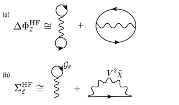
Figure 3: (a) ”Hartree-Fock” local free energy contributions and (b) corresponding self-energy diagrams. (Counter-term diagrams are not shown.) Wavy lines represent the effective interaction, $V^{2}\,\widetilde{\chi}(\tau-\tau^{\prime})$, while continuous lines stand for the unperturbed local propagator, $\mathcal{G}_{\widetilde{\varepsilon}\,}(\tau)=\langle c(\tau)\bar{c}(0)\rangle_{\rm loc}^{(0)}$, computed from the non-interacting part of Eq. (II.3) .

The effective action Eq. (II.3) describes a fermion propagating with the unperturbed propagator $\mathcal{G}_{\widetilde{\varepsilon}\,}$ associated with the first term of Eq. (II.3),

$$\mathcal{G}^{-1}_{\widetilde{\varepsilon}\,}(\tau)=\delta_{\tau,\tau^{\prime}}\left[\partial_{\tau^{\prime}}+{\widetilde{\varepsilon}\,}\right]-t^{2}\;G(\tau-\tau^{\prime}),$$ (12)

and interacting through the retarded interaction

$$V^{2}\;\tilde{\chi}(\tau-\tau^{\prime})\equiv V^{2}\;\large(\,\chi(\tau-\tau^{\prime})-\langle\delta n\rangle^{2}\large)\;.$$

To compute all needed Green’s functions and susceptibilities in a systematic way, it is convenient to formulate the approximation in terms of the the local (negative) free energy $\Phi_{\widetilde{\varepsilon}\,}$, Eq.  (11). We express $\Phi_{\widetilde{\varepsilon}\,}$ as

$$\Phi_{\widetilde{\varepsilon}\,}=\Phi^{(0)}_{{\widetilde{\varepsilon}\,}}+\Delta\Phi_{\widetilde{\varepsilon}\,}\,$$ (13)

with the second term accounting for the interaction-induced part of $\Phi_{{\widetilde{\varepsilon}\,}}$, and $\Phi^{(0)}_{{\widetilde{\varepsilon}\,}}$ being the non-interacting free energy,

$$\Phi^{(0)}_{{\widetilde{\varepsilon}\,}}=\dfrac{{\widetilde{\varepsilon}\,}}{2}+\dfrac{1}{\beta}{\rm Tr}\log\mathcal{G}_{\widetilde{\varepsilon}\,}^{-1}\;.$$ (14)

The interacting part $\Delta\Phi_{{\widetilde{\varepsilon}\,}}$ can be considered as a functional of the dressed propagator. Then its functional differential with respect to the dressed propagator is just the self-energy.

Within IPT, we simply replace the local free energy (13) by the second order perturbative expression,

$$\Delta\Phi^{\text{HF}}_{{\widetilde{\varepsilon}\,}}({\widetilde{\varepsilon}\,}) =\dfrac{V^{2}}{2}\big{(}\mathcal{G}_{\widetilde{\varepsilon}\,}(0^{-})+{1}/{2}\big{)}^{2}\int_{0}^{\beta}d\tau\,\tilde{\chi}(\tau)$$ (15)

$$-\dfrac{V^{2}}{2}\int_{0}^{\beta}d\tau\,\tilde{\chi}(\tau)\,\mathcal{G}_{\widetilde{\varepsilon}\,}(\tau)\,\mathcal{G}_{\widetilde{\varepsilon}\,}(-\tau),$$

represented by the free energy diagrams in Fig. 3(a)  . Although not constructed in terms of the full Green’s function, we shall also refer to this approximation as ”Hartree-Fock” approximation, as also inferred by the labels, ”HF”. For the self-energy, we use a similar approximation, represented in Fig. 3(b)

$$\Sigma_{\,{\widetilde{\varepsilon}\,}}^{\text{HF}}(\tau) = \delta(\tau)V^{2}\big{(}\mathcal{G}_{\,{\widetilde{\varepsilon}\,}}(0^{-})+{1}/{2}\big{)}\!\int_{0}^{\beta}\!\!d\tau^{\prime}\widetilde{\chi}_{\,{\widetilde{\varepsilon}\,}}(\tau^{\prime})$$ (16)

$$- V^{2}\widetilde{\chi}_{\,{\widetilde{\varepsilon}\,}}(\tau)\mathcal{G}_{\,{\widetilde{\varepsilon}\,}}(\tau)\;.$$

These expressions can also be obtained by functional differentiation of (15) with respect to the unperturbed propagators. The term 1/2 originates from normal ordering, and is just the average occupation.

Formally, the occupation $\langle\delta n\rangle_{\widetilde{\varepsilon}\,}$ and for the local compressibility $\chi_{\widetilde{\varepsilon}\,}(\tau)$ can be computed by inserting a time dependent energy in the action, ${\widetilde{\varepsilon}\,}\to{\widetilde{\epsilon}}_{\tau}$, and taking the functional derivatives of $\Phi_{\widetilde{\varepsilon}\,}$ with respect to ${\widetilde{\varepsilon}\,}\to{\widetilde{\epsilon}}_{\tau}$. We use this procedure to obtain the IPT expressions for the occupation $\langle\delta n\rangle_{\widetilde{\varepsilon}\,}$ and for the local compressibility $\chi_{\widetilde{\varepsilon}\,}(\tau)$, consistent with the approximations above, by just differentiating $\Phi_{\widetilde{\varepsilon}\,}^{\text{HF}}=\Phi_{\widetilde{\varepsilon}\,}^{\text{(0)}}+\Delta\Phi_{\widetilde{\varepsilon}\,}^{\text{HF}}$ as

$$\langle\delta n\rangle_{{\widetilde{\varepsilon}\,}}^{\text{HF}}=\beta\left.{\dfrac{\delta\Phi_{\widetilde{\varepsilon}\,}^{\text{HF}}}{\delta\,{\widetilde{\epsilon}}_{\tau}}}\right|_{{\widetilde{\epsilon}}_{\tau}\to{\widetilde{\varepsilon}\,}}$$ (17)

and

$$\chi^{\text{HF}}_{\,{\widetilde{\varepsilon}\,}}(\tau-\tau^{\prime})=\beta\,\left.{\dfrac{\delta^{2}\Phi_{\widetilde{\varepsilon}\,}^{\text{HF}}}{\delta\,{\widetilde{\epsilon}}_{\tau}\;\delta\,{\widetilde{\epsilon}}_{\tau^{\prime}}}}\right|_{{\widetilde{\epsilon}}_{\tau}\to{\widetilde{\varepsilon}\,}}\;.$$ (18)

The resulting expressions are quite lengthy, we therefore do not display them here, but the corresponding diagrams, shown in Fig. 4, have a quite transparent structure, and it is easy to construct the explicit formulas from them by following standard diagramatic rules.

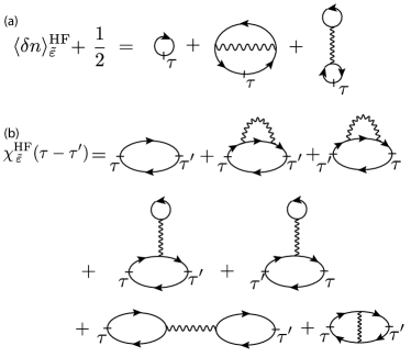
Figure 4: Hartree-Fock diagrams determining (a) the Hartree-Fock occupation, $\langle\delta n\rangle_{\text{loc}}^{\text{HF}}$, and (b) the Hartree-Fock response, $\chi_{\widetilde{\varepsilon}\,}^{\text{HF}}(\tau)$. Cuts indicate functional derivatives, counter-term diagrams are omitted.

In the RS phase, the IPT iteration is then straightforward. Assuming some ansatz for $Q_{\text{RS}}$, $\chi(\tau)$, and $G(\tau)$ we use Eq. (16) to compute $\mathcal{G}_{\widetilde{\varepsilon}\,}(\tau)$, and the diagrams in Fig. 4 to determine $\langle\delta n\rangle_{\widetilde{\varepsilon}\,}$ and $\chi_{\widetilde{\varepsilon}\,}(\tau)$ for a dense set of energies, ${\widetilde{\varepsilon}\,}$. We then determine $Q_{\text{RS}}$, $\chi(\tau)$, and $G(\tau)$ iteratively by means of Eqs. (9) and (10). In the presence of full replica symmetry breaking, the function $Q(x)$ is determined by more complicated flow equations instead of the RS expression  (10), but the rest of the iteration loop remains unaltered.

III.2 Continuous time quantum Monte Carlo

An alternative route to compute $G_{\tilde{\varepsilon}}(\tau)$, $\langle\delta n\rangle_{\tilde{\varepsilon}}$, and $\chi_{\tilde{\varepsilon}}(\tau)$ within the dynamical mean-field theory is to perform a continuous-time quantum Monte Carlo (CTQMC) computation with the effective local action $S_{{\widetilde{\varepsilon}\,}}$ given in Eq. (II.3). We use an extension of the hybridization-expansion CTQMC algorithm that can treat retarded interactions in action formalism [46, 47]. In this approach we expand the partition function $Z_{\widetilde{\varepsilon}\,}={\rm Tr}\,{\rm e}^{-S_{{\widetilde{\varepsilon}\,}}}$ in the hybridization function $F(\tau-\tau^{\prime})=t^{2}\,G(\tau-\tau^{\prime})$ while we treat the level energies $\tilde{\varepsilon}$ and interaction $V$ exactly.

In general, the hybridization-expansion CTQMC method[48, 49] relies on the expansion of the partition function $Z_{\widetilde{\varepsilon}\,}$ in the hybridization into a series of diagrams and sampling these diagrams stochastically, where $Z_{\widetilde{\varepsilon}\,}$ can be written as a sum of configurations $z_{k}$ with weight $w(z_{k})$ as $Z_{\widetilde{\varepsilon}\,}=\sum_{z_{k}}w(z_{k})$. In the segment picture a Monte Carlo configuration $z_{k}$ with expansion order $k$ is represented by $k$ segments with imaginary time intervals $\{\tau_{1},\tau^{\prime}_{1}\},...,\{\tau_{k},\tau^{\prime}_{k}\}$ where the particle number is 1, and it is 0 where there is no segment.

In our case the creation operators $\overline{c}_{\tau_{i}}$ at times $\tau_{i}$ are connected to annihilation operators $c_{\tau^{\prime}_{j}}$ at times $\tau^{\prime}_{j}$ by the hybridization function $F(\tau_{i}-\tau^{\prime}_{j})$, and the collection of these $k!$ diagrams corresponding to the hybridization lines $F$ is summed up into a determinant of a matrix $\hat{F}^{(k)}$ composed of the hybridization functions. The weight $w(z_{k})$ is expressed as $w(z_{k})={\rm det}\hat{F}^{(k)}\,w_{\tilde{\varepsilon}}\,w_{\tilde{\chi}}$ where the contributions $w_{\tilde{\varepsilon}}$ and $w_{\tilde{\chi}}$ corresponding to the level energy $\tilde{\varepsilon}$ and the interaction term $V^{2}\tilde{\chi}$ are given in Eqs. (34) and (37) in Appendix A, respectively. For further details, please visit this Appendix  A.

Since the CTQMC method is computationally very demanding, we applied it as a reference point in the RS phase. We used the extended CTQMC impurity solver in the numerical calculations with the combined weight $w(z_{k})$ by means of the Metropolis algorithm to solve the effective local action given in Eq. (II.3) for $G_{\tilde{\varepsilon}}(\tau)$, $\langle\delta n\rangle_{\tilde{\varepsilon}}$, and $\chi_{\tilde{\varepsilon}}(\tau)$ self-consistently in the Fermi-liquid (replica symmetric) phase. We proceeded to obtain the self-consistent replica symmetric solution through the following iteration steps: We may start by an arbitrary ansatz for $G^{[0]}(\tau)$, $\tilde{\chi}^{[0]}(\tau)$, and $Q^{[0]}_{\rm RS}$, for example with the non-interacting Green’s function and susceptibilities (for the explicit expressions please visit Appendix A), at the zeroth iteration step. We then compute the quantities $G^{[1]}_{\tilde{\varepsilon}}(\tau)$, $\tilde{\chi}^{[1]}_{\tilde{\varepsilon}}(\tau)$, and $\langle\delta n\rangle_{\tilde{\varepsilon}}$ at the subsequent iteration step with the effective local action, Eq. (II.3), using the CTQMC impurity solver for a wide range of level energies $\tilde{\varepsilon}$. The averaged quantities $G^{[1]}(\tau)$, $\tilde{\chi}^{[1]}(\tau)$, and $Q^{[1]}_{\rm RS}$ are obtained by (numerical) integration over $\tilde{\varepsilon}$ with the distribution $\tilde{P}(\tilde{\varepsilon})$ as it is given in Eqs. (9) and (10). They are used for the next iteration step, and we repeat this procedure until we reach convergence.

We calculated several points of the phase boundary by CTQMC using the stability condition given in Eq. (20) below for various parameter values for $t$, $V$ and $T$, and found excellent agreement between the IPT and CTQMC calculations. The spectral functions are also compared and found to show similar energy dependence between IPT and CTQMC. However, around zero energy $\omega\sim 0$ difference arises in the density of states between the IPT and the numerically exact solution as we approach the glassy phase by increasing the interaction $V$, or decreasing the hopping $t$.

IV Replica symmetric spectral functions and phase boundary

We used both approaches described in the previous section to compute the Green’s function $G(\tau)$ and the susceptibility $\tilde{\chi}(\tau)$ in the replica symmetric phase. The average local tunneling density of states (DOS) can then be computed from the Fourier transform $G(i\omega)$ as

$$\rho(\omega)=\dfrac{1}{\pi}\,{\rm Im}G(i\omega\to\omega+i\,0^{+})\;.$$ (19)

In the very last step, we have used a Padé construction to carry out the analytical continuation.

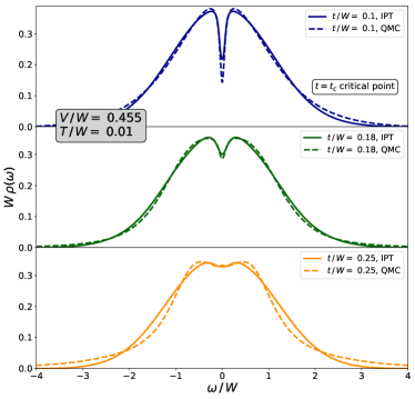
Figure 5: Average low temperature density of states in the Fermi liquid phase, as computed by CTQMC and by IPT. The density of states develops a remarkable zero bias anomaly already in the Fermi liquid, though the distribution of Hartree levels is still featureless. Increasing quantum fluctuations wash away this correlation hole.

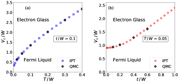
Figure 6: Phase boundary between the electron glass and the Fermi liquid, as computed by continuous time Monte Carlo and IPT along the lines indicated in Fig. 2. Interactions lead to the formation of the glass. Quantum fluctuations as well as thermal fluctuations melt the electron gas.

Fig. 5 shows the spectral functions in the Fermi liquid phase for a moderate interaction, $V/W=0.455$, and quite small temperature, $T/W=0.01$, as we drive the system closer and closer to the Fermi liquid - electron glass quantum phase transition. For large $t$, quantum fluctuations destroy the electron glass, and a dirty Fermi liquid is formed. There the density of states is almost featureless. As we decrease $t/W$, quantum fluctuations get suppressed, and a plasma dip structure starts to form in the middle of the band, even though the system still remains in the replica symmetric Fermi liquid phase. IPT and CTQMC are in very good agreement, and yield both very similar structures. Differences can be attributed to the approximations made within IPT, to the limited CTQMC accuracy, and to uncertainties related to the analytical continuation.

The presence of a plasma dip (or correlation hole) in the Fermi liquid phase reflects short range charge correlations due to the repulsive interactions between neighboring sites. This correlation hole is a manifestation of Onsager’s back reaction, and it is not directly related to the Efros-Shklovskii gap of the glassy phase [33, 34]. Indeed, in the liquid phase, replica symmetry is maintained, implying that the distribution of the renormalized Hartree-Fock levels, $\tilde{P}(\tilde{\epsilon})$ is still a featureless Gaussian, in contrast to the tunneling density of states.

The boundary of the electron glass phase is determined by a stability (marginality) condition against replica symmetry breaking, ensuring the stability of the solution $Q_{ab}\equiv Q_{\rm RS}$. This is essentially identical to the stability condition appearing in the SK model [23],

$$1=V^{2}\int\,\text{d}{\widetilde{\varepsilon}\,}\,\widetilde{P}_{\text{RS}}({\widetilde{\varepsilon}\,})\,\chi_{\rm stat}^{2}({\widetilde{\varepsilon}\,}),$$ (20)

with the static local susceptibility defined as $\chi_{\rm stat}({\widetilde{\varepsilon}\,})\equiv\partial_{\widetilde{\varepsilon}\,}\langle\delta n\rangle_{\widetilde{\varepsilon}\,}$.

The resulting phase diagram has been presented in Fig. 2 for a finite disorder, $W$. At any temperature and for any hopping $t$, replica symmetry is broken at interactions larger than some critical value, $V\geq V_{C}(T,t,W)$. In the classical limit, $t=0$, in particular, an interaction-driven glass phase emerges at low temperatures for small disorder. Contrary to naive expectations, strong disorder destroys the glassy phase, and leads to a trivial strongly disordered phase without replica symmetry breaking (RSB): fluctuations of the bare levels $\varepsilon_{i}$ are so large that each level becomes occupied or unoccupied essentially independently, leaving no room to interaction-induced frustration. For sufficiently strong interaction, however, a Coulomb glass phase emerges.

The glass phase can be destroyed not only by extreme disorder, but also by thermal and quantum fluctuations, induced by the temperature, $T$, or the tunneling, $t$. This is demonstrated in the cuts shown in Fig. 6 (indicated as dashed lines in Fig. 2), where we also compare the CTQMC results with those of IPT. The excellent agreement of these two approaches validates the latter, approximate method.

The role of thermal and quantum fluctuations is not quite identical. In the classical ($t\to 0$) limit, $V_{C}^{\text{class}}\sim\sqrt{T\,W}$, while in the quantum case ($T\to 0$), the escape rate $\Gamma\sim t^{2}/W$ takes over the role of the temperature, and $V_{C}^{\text{quant}}\sim t$.

At finite temperatures, quantum fluctuations and thermal fluctuations compete with each other. As demonstrated in Fig. 6(b), at a finite temperatures, small quantum fluctuations with $\Gamma\lesssim T$ do not change the critical interaction strength, $V_{C}$, and the transition is mostly induced by just thermal fluctuations. For $\Gamma\gtrsim T$, i.e., $t/W\gtrsim\sqrt{T/W}$, however, quantum fluctuations play the dominant role, as evidenced by the almost linear shift of $V_{C}$ with increasing $t/W$.

V Electron glass phase: full replica symmetry breaking

The exact solution of the self-consistency equations in the presence of full replica symmetry breaking is a demanding task. One first needs to solve the non-local quantum impurity problem, Eq. (II.3) for a relatively large set of ${\widetilde{\varepsilon}\,}$ values, extract the expectation values $\langle\delta n\rangle_{{\widetilde{\varepsilon}\,}}$ as well as the dressed local Green’s functions and susceptibilities. Then one needs to solve the above-mentioned flow equations in replica space to update the distribution $\widetilde{P}({\widetilde{\varepsilon}\,})$, compute the average susceptibilities and Green’s functions using (9), and then close the cycle by Eq. (II.3). Although this is, in principle, possible at a given point in parameter space using, e.g., continuous time quantum Monte-Carlo methods [50], it appears to be unavoidable to use an approximate scheme such as IPT if one aims at determining the complete phase diagram. Below, we summarize the results of IPT computations. Further CTQMC results shall be published elsewhere [50].

V.1 Overlap distribution

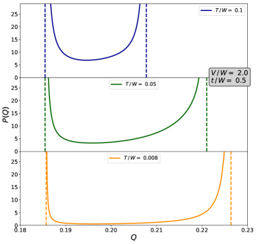
Figure 7: Overlap distribution $P(Q)$ in the electron glass phase, as a function of temperature.

The differential of the inverse function $x(Q)$ turns out to be just the distribution of the overlaps between different replicas,

$$Q^{ab}=\lim_{N\to\infty}{\frac{1}{N}\sum_{i}\langle\delta n_{i}\rangle_{a}\langle\delta n_{i}\rangle_{b}}\;,$$

$$P(Q^{ab}=Q)=\frac{\text{d}x}{\text{d}Q}\;.$$ (21)

The numerically computed function $P(Q)$ is presented in Fig. 7. In the Fermi liquid phase (not shown), $P(Q)$ is trivial, and consists of a delta function, $P^{\text{RS}}(Q)=\delta(Q-Q_{\text{RS}})$. This distribution indicates a unique, symmetric mean field solution. In the electron glass phase, the distribution becomes non-trivial, and possible overlaps have a range, $Q\in[Q_{\text{min}},Q_{\text{max}}]$, showing the onset of many symmetry-broken states. This overlap window becomes broader and broader as the temperature is lowered, and at the same time, the distribution gets depleted, and has a hight $\sim T$. This is in line with the observation, that at $T=0$ temperature, replica symmetry is restored. (It is, however, not so clear if a valid expansion around this limit exists [29].) Notice that the maximal value, $Q_{\text{max}}(T\to 0)$ remains less than $1/4$; this is a consequence of quantum fluctuations, which tend to reduce the overlaps.

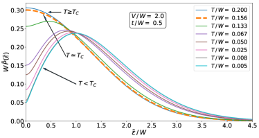
Figure 8: Formation of the pseudogap in the distribution ${\widetilde{P}\,}({\widetilde{\varepsilon}\,})$ as a function of temperature. At $T>T_{C}$ the distribution remains Gaussian, but as we decrease the temperature below $T_{C}$ a pseudogap develops gradually. The thick dashed line represents the distribution at the critical temperature $T=T_{C}$.

V.2 Distribution of Hartree-Fock levels and tunneling spectra

As in classical spin glasses [19, 34, 33], a clear signature of the glass transition is the emergence of a Coulomb gap structure in the distribution of Hartree-Fock energies, $\widetilde{P}({\widetilde{\varepsilon}\,})$, shown in Fig. 8. The Coulomb gap starts to open up gradually after crossing the phase transition, and a fully developed Coulomb gap appears only deep in the glassy phase [51]. Although the pseudogap gets deeper and deeper as the temperature decreases, $\widetilde{P}({\widetilde{\varepsilon}\,}=0)$ remains finite even at $T=0$ temperature for any finite $t$. This is a property of the infinite coordination limit, $z\to\infty$, where Anderson localization is absent, and a disordered metal state emerges in the absence of interactions at $T=0$ temperature. Nevertheless, interactions larger than a critical value drive a phase transition to a replica symmetry broken phase, where the density of states is strongly suppressed but finite even at $T=0$ temperature. We can interpret this phase as a metallic Coulomb glass.

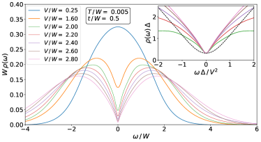
Figure 9: (Main panel) Evolution of the density of states for various interaction strengths $V$. The critical coupling is $V_{c}\approx 1.31\,W$. When $V>V_{C}$ a pseudogap appears in $\varrho(\omega)$, that grows with increasing V, but the density of states at the Fermi level $\varrho(0)$ always remains finite. (Inset) Universal collapse of $\varrho(\omega)$. The dashed curve indicates the scaling curve in the classical limit, $t\to 0$.

While the distribution of the renormalized energies ${\widetilde{\varepsilon}\,}$ is conceptually interesting, excepting the classical limit, their distribution is not directly measurable. What is, however, measurable is the tunneling density of states at a given site of renormalized energy, ${\widetilde{\varepsilon}\,}$,

$$\rho_{\widetilde{\varepsilon}\,}(\omega)=\dfrac{1}{\pi}\,{\rm Im}G_{\widetilde{\varepsilon}\,}(\omega^{+})\;,$$ (22)

and the average density of states, $\rho(\omega)=\,{\rm Im}G(\omega^{+})/\pi$,

$$\rho(\omega)=\int\text{d}{\widetilde{\varepsilon}\,}\;\rho_{\widetilde{\varepsilon}\,}(\omega)\;\tilde{P}({\widetilde{\varepsilon}\,})\,\;.$$ (23)

Fig. 9 shows the formation of the pseudogap in $\rho(\omega)$ at very small temperatures, as interactions are increased. The density of states at the Fermi energy is finite, and defines a natural energy scale $\Delta\equiv\varrho^{-1}(0)$. This scale becomes smaller and smaller upon increasing interactions, while $\rho(\omega)$ develops universal scaling as a function of $\omega\cdot\Delta/V^{2}$ at low energies, where it crosses over from a constant to a linear regime, $\rho(\omega)\propto\omega/V^{2}$ (see inset in Fig. 9). Notice that the presence of disorder does not influence this slope, also indicating that the phase transition we observe is driven by interactions and not by disorder. The classical scaling function corresponding to $t=0$, also displayed in the inset of Fig. 9, yields the same slope as the quantum version, but the two scaling functions clearly differ, thereby demonstrating the difference between the role of thermal and quantum fluctuations. As shown in Appendix  C, the distribution ${\widetilde{P}\,}({\widetilde{\varepsilon}\,})$ exhibits similar universal scaling structure.

It is instructive to investigate the structure of individual tunneling spectra, $\rho_{\widetilde{\varepsilon}\,}(\omega)$, shown for a set of levels deep in the quantum glass regime in Fig. 10. The local density of states displays peaks at around the renormalized level, ${\widetilde{\varepsilon}\,}$, which is broadened by quantum fluctuations. Levels close to the Fermi level become sharp since surrounding sites have a suppressed density of states at the pseudogap.

VI Thermodynamics

To determine the free energy of the glass we first need to determine the (negative) free energy density $\Phi_{\rm loc}(T)$ of the effective replica action $S_{\rm rep}$, Eq. (II.2),

$$\Phi_{\text{loc}}(T)\equiv\lim_{n\to 0}\frac{1}{n}k_{B}T\,\log\,\bigg{\{}\int\mathcal{D}\overline{c}\,\mathcal{D}c\;e^{-S_{\rm rep}[\,\overline{c},c\,]}\,\bigg{\}}\;.$$ (24)

This is slightly different from the physical free energy density of the lattice model, Eq. (1), which we denote by $\Phi_{\rm phys}(T)$, since we must restore some terms that we threw away in course of the Hubbard-Stratonovic transformation. Restoring these terms, which depend on the local Green’s function and susceptibility, we obtain

$$\Phi_{\rm latt}(T) =\Phi_{\rm loc}(T)+\dfrac{t^{2}}{2}\int_{0}^{\beta}{\rm d}\tau\,G(\tau)G(-\tau)$$

$$-\dfrac{V^{2}}{4}\int_{0}^{\beta}{\rm d}\tau\,\chi(\tau)^{2}-\dfrac{\beta V^{2}}{4}\dfrac{1}{n}\sum_{b\neq a}Q_{ab}Q_{ba}.$$ (25)

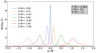
Figure 10: Unaveraged density of states deep in the glass phase for various values of ${\widetilde{\varepsilon}\,}$.

In the replica symmetrical (Fermi liquid) case, Eq.(24) simplifies, and we obtain

$$\Phi_{\text{loc}}^{\text{\,RS}}(T)=\int\text{d}{\widetilde{\varepsilon}\,}\,{\widetilde{P}\,}_{\text{RS}}({\widetilde{\varepsilon}\,})\,\Phi_{\widetilde{\varepsilon}\,}(T),$$ (26)

with the free energy $\Phi_{\widetilde{\varepsilon}\,}(T)$ computed from the local effective action, Eq. (II.3), and ${\widetilde{P}\,}_{\text{RS}}$ the Gaussian Hartree level distribution, displayed below Eq. (II.3). In this case, the last term of (VI) also simplifies to

$$-\frac{1}{n}\dfrac{\beta V^{2}}{4}\sum_{b\neq a}Q_{ab}Q_{ba}\to\beta\frac{V^{2}}{4}Q_{\text{RS}}^{2}\;$$

in the $n\to 0$ limit, yielding a complete expression for the lattice Free energy.

This procedure can be extended to the glassy phase, too, as outlined in Appendix  B, only the computation of $\Phi_{\rm loc}(T)$ becomes more complex, since one cannot decouple replicas with a single Hubbard-Stratonovich transformation. One still has to solve local effective action $S_{\widetilde{\varepsilon}\,}$ at the start, (with $\tilde{\chi}=\chi-Q_{\text{RS}}$ replaced by $\chi-Q(1)$), and solve the so-called flow equations in replica space (see Appendix  B for details) to obtain an expression for $\Phi_{\text{loc}}(T)$ analogous to Eq. (26).

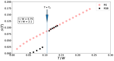
Figure 11: Temperature dependence of the entropy for the replica symmetric (RS) and replica symmetry beaking (RSB) solution. The RSB solution indicates an entropy scaling to zero as $T\rightarrow 0$. Since we can not access the immediate vicinity of the critical temperature $T_{C}$ with the RSB calculation, $\mathcal{S}(T)$ can not distinguish between a continuous phase transition and a first order entropy jump at $T_{C}$.

Once $\Phi_{\text{loc}}(T)$ and the converged Green’s functions and the order parameter $Q(x)$ at hand, the thermodynamic quantities of the lattice model can then be computed from $\Phi_{\rm latt}(T)$. In particular, we determined the temperature dependent entropy density $\mathcal{S}(T)$, given by

$$\mathcal{S}=\dfrac{\partial\Phi_{\text{latt}}}{\partial T}.$$ (27)

Our results for $\mathcal{S}(T)$ are displayed the temperature dependent entropy $\mathcal{S}(T)$ in Fig. 11. Although we cannot decrease the temperature very deep down into the RSB phase, the numerical data are consistent with the entropy remaining positive and going quadratically to zero as $T\rightarrow 0$, corresponding to a quadratic specific heat.

Calculating the entropy $\mathcal{S}(T)$ numerically in the vicinity of the phase boundary is very challenging, due to the slow convergence of the iterative solution in the RSB phase, as well as because of the difficulties in evaluating the numerical derivative in Eq. (27) with high enough precision. For these reasons, we were unable to determine $\mathcal{S}(T)$ in the immediate vicinity of the critical temperature $T_{C}$, preventing us from answering the extremely difficult question about the order of the phase transition. The results plotted in Fig. 11 are consistent either with a continuous phase transition or with a weakly first order transition with a latent heat.

Figure 12: Overlap $Q$ across the glass transition. We plot the RS solution $Q_{RS}$, as well as the RSB results $Q_{RSB}(1)$ and $Q_{RSB}(0)$ as a function of interaction strength $V$. The glass order parameter $Q_{RSB}(1)-Q_{RSB}(0)$ remains continuous at the phase boundary, pointing towards a continuous phase transition.

We can gain more insight into the properties of the glass transition by examining the behavior of the overlap function $Q(x)$ across the phase boundary. We show the RS prediction $Q_{RS}$, as well as the RSB results $Q_{RSB}(1)$ and $Q_{RSB}(0)$ as a function of interaction strength $V$ in Fig. 12. We find that $Q_{RSB}(1)-Q_{RSB}(0)$, serving as an order parameter for the glass transition, changes continuously at the phase boundary. Similarly, the distribution ${\widetilde{P}\,}$ is apparently continuous through the Coulomb glass phase transition. We also note that we do not see any evidence for a mixed phase between the RS and RSB regimes in our numerical simulations, which could signal a first order phase transition. These findings point towards a continuous Coulomb glass transition, despite the somewhat inconclusive results in Fig. 11. We note that various previous studies have relied on the assumption of a continuous phase transition, by applying Landau theory to examine the glass transition [27, 28].

VII Discussion

We presented here a detailed study of the mean field Coulomb glass (disordered $t-V$) model of Ref. [23] in the quantum regime, in the Fermi liquid (replica symmetrical) as well as deep in the glassy (replica symmetry) broken phase. The combination of continuous time quantum Monte-Carlo approach with Iterative Perturbation Theory (IPT) allowed us to map accurately the phase boundaries separating the interaction induced glassy phase from the Fermi liquid phase in the classical as well as in the quantum regime, and to determine spectral functions as well as thermodynamic properties. Having validated our IPT scheme in the metallic regime, we used it to enter the electron glass phase, where complete replica symmetry breaking must be incorporated in the theory.

In the spectral function, we observe the formation of a plasmonic correlation hole in the average tunneling density (local density of states) already in the Fermi liquid phase. This correlation hole smoothly develops into an Efros-Shklovskii pseudogap when we enter the electron glass phase, where replica symmetry is broken. The Efros-Shklovskii pseudogap gap is, however, not fully developed in this mean field model even at $T=0$ temperature: similar to thermal fluctuations, small quantum fluctuations induce a finite density of states even at the Fermi energy. This is a peculiarity of the infinite coordination limit, where Anderson localization is absent, and a glassy Fermi liquid state emerges rather than a glassy localized phase. For small tunneling, the average density of states exhibits universal scaling at at low temperatures and low energies. Similar features have been observed in the transverse field Sherrington-Kirkpatrick model in Ref. [35].

We have also computed the local density of states. In the electron glass phase, this typically consists of sharp resonances, located around some renormalized Hartree energies, whose distribution also exhibits a pseudogap. These resonances become sharper and sharper as one approaches the Fermi energy, but retain their finite width, even at the Fermi surface, indicating again that these states remain extended even in the glass phase.

We have also constructed the full thermodynamic mean field description of the disordered $t-V$ model, and analyzed its thermodynamic properties in both phases. We obtain a continuous free energy, however, our present results are not yet accurate enough to distinguish between a continuous phase transition and a first order entropy jump. While the entropy calculation remains inconclusive, the apparent continuous behavior of the glass order parameter at the phase boundary, as well as the lack of numerical evidence for a mixed phase characteristic of first order transitions, points towards a continuous glass transition, in accordance with the results of a Landau functional approach [27, 28]. Further, very accurate continuous time quantum Monte-Carlo computations for the entropy within the replica symmetry broken phase could provide more evidence for this conclusion.

As mentioned above, the absence of the insulating electron glass phase is an artifact of the infinite coordination limit. However, the unavoidably metallic glass phase emerging in this model is relevant for many metallic disordered systems, which exhibit glassy behavior. Amorphous polycrystaline solids [11] or granular metals [52] are such examples, but metallic electron glass phases can be observed in certain two dimensional systems [31, 53]. Thorough studies of $\rm{Na}^{+}$ doped silicon MOSFETs reveal a metal insulator transition at a carrier density, $n\approx n_{c}$, and an intermediate metallic glass phase emerges on the metallic side of the transition at concentrations $n_{g}>n>n_{c}$, as evidenced by low frequency resistance noise [53] and ageing [8] experiments on low mobility samples. A metallic glass phase could also be experimentally realized in ultracold atomic settings, by placing fermionic atoms into a multi-mode cavity  [39].

The understanding and solution of the mean field Coulomb glass model, Eq. (1), is just a first step in constructing a mean field theory of the real Coulomb glass. In fact, it is quite unclear, how one could incorporate localization and long-ranged interactions at the same time in a mean field model. To have an Anderson-localized phase, one should impose a finite coordination number, $z$, and thereby exclude the presence of infinite number of nearest neighbors. This challenging problem can be studied via an extended dynamical mean field theory (EDMFT) approach [55] and a coherent potential approximation (CPA), allowing to use the present scheme as a local approximation to describe the glassy phase transition in a finite dimensional system [34]. Alternatively, Anderson localization can also be captured by combining DMFT arguments with a typical medium theory (TMT) scheme [56].

Another open question is that of glassy dynamics. Global charge response should reflect the emergence of a glassy phase through anomalously slow response and a broad distribution of scales [9, 10]. It remains an open question, how the present approach is able to explain this behavior. Finally, spin degrees of freedom have been completely neglected in this work. The role of Mott-Anderson physics and spontaneous spin formation should be further explored and elucidated.

Although in this work we only focused on the description of the Coulomb glass phase, the method and formalism presented pave the way to study quantum correlations in the glassy phase of many mean field quantum glass models, such as the transverse field Sherrington-Kirkpatrick model, and the disordered Dicke model. All these questions are and should be subject of future research.

Appendix A Details of continuous time quantum Monte Carlo method

In this appendix we present the derivation of the combined Monte Carlo weight $w(z_{k})={\rm det}\hat{F}^{(k)}\,w_{\tilde{\varepsilon}}\,w_{\tilde{\chi}}$ based on the implementation presented in Ref. [46].

We separate the effective local action given in Eq. (II.3) as

$$S_{{\widetilde{\varepsilon}\,}} \equiv S_{\rm F}+S_{1},$$ (28)

$$S_{\rm F} = -\int_{\tau}\int_{\tau^{\prime}}\overline{c}_{\tau}t^{2}\;G(\tau-\tau^{\prime})\;c_{\tau^{\prime}},$$ (29)

$$S_{1} = \int_{\tau}\overline{c}_{\tau}(\partial_{\tau}+\tilde{\varepsilon})c_{\tau}$$ (30)

$$- \frac{V^{2}}{2}\int_{\tau}\int_{\tau^{\prime}}\large(\chi(\tau-\tau^{\prime})-Q_{\text{RS}}\large)\;\delta n_{\tau}\;\delta n_{\tau^{\prime}},$$

and expand the partition function $Z_{\widetilde{\varepsilon}\,}={\rm Tr}\,{\rm e}^{-S_{{\widetilde{\varepsilon}\,}}}$ in terms of the hybridiztion part $S_{\rm F}$, which gives

$$Z_{\widetilde{\varepsilon}\,} = {\rm Tr}\,{\rm e}^{-(S_{\rm F}+S_{1})}=$$

$$= \sum_{k}\int_{0}^{\beta}dt\tau_{1}...d\tau_{k}\int_{0}^{\beta}dt\tau^{\prime}_{1}...d\tau^{\prime}_{k}\,{\rm det}\hat{F}^{(k)}$$

$$\times {\rm Tr}\left[\,{\rm e}^{-S_{1}}\,\overline{c}_{\tau_{1}}c_{\tau^{\prime}_{1}}...\overline{c}_{\tau_{k}}c_{\tau^{\prime}_{k}}\right]=\int{\cal D}(k)w(z_{k}),$$ (32)

where we introduced the notation $\int{\cal D}=\sum_{k}\int_{0}^{\beta}dt\tau_{1}...d\tau_{k}\int_{0}^{\beta}dt\tau^{\prime}_{1}...d\tau^{\prime}_{k}$, and therefore the weight $w(z_{k})$ is expressed as

$$w(z_{k}) = {\rm det}\hat{F}^{(k)}\,{\rm Tr}\,\left[{\rm e}^{-S_{1}}\,\overline{c}_{\tau_{1}}c_{\tau^{\prime}_{1}}...\overline{c}_{\tau_{k}}c_{\tau^{\prime}_{k}}\right]$$ (33)

$$= {\rm det}\hat{F}^{(k)}\,\langle\overline{c}_{\tau_{1}}c_{\tau^{\prime}_{1}}...\overline{c}_{\tau_{k}}c_{\tau^{\prime}_{k}}\rangle.$$

By evaluating the first term of $S_{1}$ in Eq. (30) in the segment picture, we obtain the weight $w_{\tilde{\varepsilon}}$ as

$$w_{\tilde{\varepsilon}}={\rm e}^{-\tilde{\varepsilon}\,l},$$ (34)

where $l=\sum_{i=1}^{k}l_{i}$ is the total length of the segments $l_{i}$ with $l_{i}=\tau_{i}-\tau^{\prime}_{i}$.

The weight contribution from the second term in Eq. (30) is expressed as

$$w_{\tilde{\chi}} = {\rm e}^{\frac{1}{2}V^{2}\int_{0}^{\beta}d\tau_{1}\int_{0}^{\beta}d\tau_{2}\tilde{\chi}(\tau_{1}-\tau_{2})\,\delta n_{\tau_{1}}\delta n_{{\tau^{\prime}_{2}}}}.$$ (35)

Defining a function $K(\tau)$ as $K(\tau)^{\prime\prime}=V^{2}\tilde{\chi}(\tau)$ with the conditions $K(0)=0$ and $K^{\prime}(0)=1/2V^{2}\int_{0}^{\beta}d\tau\tilde{\chi}(\tau)$, the integral in Eq. (35) is evaluated as

$$w_{\tilde{\chi}} = {\rm exp}\biggl{(}\frac{1}{2}\sum_{k_{1},k_{2}}\left[-K(\tau_{k_{1}}^{\prime}-\tau_{k_{2}}^{\prime})+K(\tau_{k_{1}}-\tau_{k_{2}}^{\prime})\right.\biggl{.}$$ (36)

$$+ \biggl{.}\left.K(\tau_{k_{1}}^{\prime}-\tau_{k_{2}})-K(\tau_{k_{1}}-\tau_{k_{2}})\right]\biggr{.}$$

$$+ \biggr{.}K^{\prime}(0)l(1-2\langle n\rangle)\biggr{)},$$

which can be rewritten as

$$w_{\tilde{\chi}} = {\rm exp}\biggl{(}-\sum_{i>j}s_{i}s_{j}[K(\tilde{\tau}_{i}-\tilde{\tau}_{j})-K(0)]\biggr{.}$$ (37)

$$+ \biggl{.}K^{\prime}(0)l(1-2\langle n\rangle)\biggr{)}$$

$$= {\rm exp}\left(-\sum_{i>j}s_{i}s_{j}K(\tilde{\tau}_{i}-\tilde{\tau}_{j})\right),$$

where the times are ordered as $0<\tilde{\tau}_{1}<\tilde{\tau}_{2}<...<\beta$, and $s$ is $+1$ for a creation operator and $-1$ for annihilation operator. Thus, $w(z_{k})$ can finally be expressed in the compact form $w(z_{k})={\rm det}\hat{F}^{(k)}\,w_{\tilde{\varepsilon}}\,w_{\tilde{\chi}}$. We note that quantities can be measured without additional computation cost compared to the case of $V=0$ with this modified weight.

The Green’s function $G(\tau)=\langle T_{\tau}\,c(0)\,\overline{c}(\tau)\rangle$ is evaluated in the same way in our Monte Carlo procedure as in the absence of the retarded interaction $V^{2}\tilde{\chi}(\tau-\tau^{\prime})$. Namely, for measuring the Green’s function we need a configuration where operators $c_{\tau^{\prime}}$ and $\overline{c}_{\tau}$ are unconnected. In the hybridization method this is achieved by removing one of the hybridization lines, resulting in

$$G(\tau)=\left\langle\frac{1}{\beta}\sum_{i,j}^{k}\left(\hat{F}^{(k)}\right)^{-1}_{ji}\tilde{\delta}(\tau,\tau_{i}-\tau^{\prime}_{j})\right\rangle_{\rm MC}.$$ (38)

Here $F_{i,j}^{(k)}=F(\tau_{i}-\tau^{\prime}_{j})$ is the hybridization matrix, and we have defined

$$\tilde{\delta}(\tau,\tau^{\prime})=\begin{cases}\delta(\tau-\tau^{\prime})&{\rm if}\quad\tau^{\prime}>0\\ -\delta(\tau-\tau^{\prime})&{\rm if}\quad\tau^{\prime}<0.\end{cases}$$

Both averaged susceptibilities $\chi(\tau)=\langle\delta n_{\tau}\delta n_{0}\rangle$ and $\tilde{\chi}(\tau)=\langle n_{\tau}n_{0}\rangle-\langle n\rangle^{2}$ can be sampled in the Monte Carlo simulation, and therefore the properties $\chi(\tau=0)=1/4$, $\tilde{\chi}(\tau=0)=1/4-q_{\rm RS}$, and $\tilde{\chi}(\tau)=\chi(\tau)-q_{\rm RS}$ can be check-points for the correctness of the CTQMC code.

Our choice for the zeroth order ansatz for $G^{[0]}(\tau)$, $\tilde{\chi}^{[0]}(\tau)$, and $Q^{[0]}_{\rm RS}$ in obtaining the self-consistent replica symmetric solution are the non-interacting ones as

$$G^{[0]}(i\omega_{n}) = i\frac{1}{2t^{2}}\left(\omega_{n}-\sqrt{4t^{2}+\omega_{n}}\right)$$ (39)

$$\xrightarrow[]{\text{FFT}}\,G^{[0]}(\tau),$$

$$\tilde{\chi}^{[0]}(\tau) = G^{[0]}(\tau)G^{[0]}(-\tau),$$ (40)

$$Q^{[0]}_{\rm RS} = 0.$$ (41)

We note that the choice of the ansatz does not affect the converged result.

Appendix B Replica symmetry breaking

In the glassy phase, replica symmetry is broken, and $Q^{ab}$ acquires a non-trivial structure in replica space. In the limit $n\to 0$, we characterize the matrix $Q^{ab}$ in terms of a continuous variable, $x\in[0,1]$, and a corresponding function, $Q_{ab}\rightarrow Q(x)$. The parameter $x$ in this language characterizes deeper and deeper levels of replica symmetry breaking as $x$ flows from 0 towards 1.

As stated in the main text, the simple construction leading to Eqs. (II.3) and  (9) can be generalized to this more complicated case, too. Following steps similar to those in Refs. [54, 34], we can introduce a set of effective one level models (actions), parametrized by $x$, and describing different levels of replica symmetry breaking, restricted free energy densities, $\phi_{{\widetilde{\varepsilon}\,},x}(T)$, and corresponding level distributions, $P_{x}({\widetilde{\varepsilon}\,})$, both temperature dependent quantities.

There is a trade-off between these two quantities: at $x=1$, $\phi_{{\widetilde{\varepsilon}\,},x}$ simplifies to

$$\phi_{{\widetilde{\varepsilon}\,},x=1}=\Phi_{\widetilde{\varepsilon}\,}(T)=\dfrac{1}{\beta}\log Z_{{\widetilde{\varepsilon}\,}},\\$$ (42)

where $Z_{{\widetilde{\varepsilon}\,}}$ is computed from the effective action, Eq. (II.3), with

$$\tilde{\chi}(\tau-\tau^{\prime})\equiv\chi(\tau-\tau^{\prime})-Q(1).$$ (43)

At the same time, the distribution ${\widetilde{P}\,}_{x\to 1}({\widetilde{\varepsilon}\,})$ has a complicated, renormalized form

$${\widetilde{P}\,}_{x\to 1}({\widetilde{\varepsilon}\,})\equiv{\widetilde{P}\,}({\widetilde{\varepsilon}\,}),$$ (44)

i.e., the distribution, which enters the computation of the average Green’s function.

In contrast, for $x=0$, the distribution ${\widetilde{P}\,}_{x\to 0}({\widetilde{\varepsilon}\,})$ becomes just the bare distribution of levels (without replica symmetry breaking), with $Q_{\text{RS}}$ replaced by $Q_{0}\equiv Q(0)$,

$${\widetilde{P}\,}_{x\to 0}({\widetilde{\varepsilon}\,})\equiv P_{0}({\widetilde{\varepsilon}\,})=\dfrac{\exp\left\{-{\widetilde{\varepsilon}\,}^{2}/\left(2\left[W^{2}+V^{2}Q_{0}\right]\right)\right\}}{\sqrt{2\pi\left[W^{2}+V^{2}Q_{0}\right]}}\;,$$ (45)

while $\phi_{{\widetilde{\varepsilon}\,},x=0}$ incorporates all scales of replica symmetry breaking in the range $x\in[0,1]$, and is directly related to the physical (negative) free energy density of the local replica action $S_{\rm rep}$, $\Phi_{\text{loc}}(T)$, as

$$\Phi_{\text{loc}}(T)=\int\text{d}{\widetilde{\varepsilon}\,}\;P_{0}({\widetilde{\varepsilon}\,})\,\phi_{{\widetilde{\varepsilon}\,},x=0}\,.$$ (46)

The distributions $P_{{\widetilde{\varepsilon}\,},x}$ and the free energies $\phi_{{\widetilde{\varepsilon}\,},x}$ at different layers of replica symmetry breaking are related by flow equations, which we can derive following the lines of Refs. [34, 33, 54] . This relation is expressed in terms of simple partial differential equations:

$$\partial_{x}\phi_{{\widetilde{\varepsilon}\,},x}=-\dfrac{V^{2}}{2}\dfrac{dQ}{dx}\left\{\partial_{\widetilde{\varepsilon}\,}^{\,2}\,\phi_{{\widetilde{\varepsilon}\,},x}+\beta x\left(\partial_{\widetilde{\varepsilon}\,}\phi_{{\widetilde{\varepsilon}\,},x}\right)^{2}\right\},$$ (47)

$$\partial_{x}P=\dfrac{V^{2}}{2}\dfrac{dQ}{dx}\left\{\partial_{\widetilde{\varepsilon}\,}^{\,2}P-2\beta x\,\partial_{\widetilde{\varepsilon}\,}\left(P\partial_{\widetilde{\varepsilon}\,}\phi_{{\widetilde{\varepsilon}\,},x}\right)\right\}.$$ (48)

These equations just express the fact that one can determine $\phi_{{\widetilde{\varepsilon}\,},x}$ and $P_{x}({\widetilde{\varepsilon}\,})$ at a ”deeper” RSB level, $x-\text{d}x$, from the knowledge of the energy dependent free energy at level $x$ and the corresponding distribution, $P(x,{\widetilde{\varepsilon}\,})$.

Finally, $Q(x)$ is determined from the last equation of the self-consistency condition Eq. (7), coinciding with the marginality condition, which ensures that the free energy is marginal with respect to all variations of $Q(x)$. This leads to the self-consistency equation,

$$Q(x)=\int\,d{\widetilde{\varepsilon}\,}P_{\widetilde{\varepsilon}\,}(x)\left[\partial_{\widetilde{\varepsilon}\,}\phi_{{\widetilde{\varepsilon}\,},x}\right]^{2}.$$ (49)

Using IPT, the solution thus proceeds as follows: Having some ansatz for $G(\tau)$, $\widetilde{\chi}(\tau)$, and $Q(x)$, we first solve the action $S_{\widetilde{\varepsilon}\,}$ in Eq. (II.3) within the Hartree-Fock approximation, and determine $\Phi_{{\widetilde{\varepsilon}\,},x=1}=\Phi_{\widetilde{\varepsilon}\,}$ for a dense set of levels ${\widetilde{\varepsilon}\,}$’s. We then solve Eq. (47) backwards, from $x=1$ to $x=0$ to obtain an estimate for $\Phi_{{\widetilde{\varepsilon}\,},x}$. Using $\Phi_{{\widetilde{\varepsilon}\,},x}$, we can now solve Eq. (48) to obtain the distributions $P_{x}({\widetilde{\varepsilon}\,})$ from $P_{x=0}({\widetilde{\varepsilon}\,})$. We then use $P_{(}{\widetilde{\varepsilon}\,})$ together with $\Phi_{{\widetilde{\varepsilon}\,},x}$ to estimate $Q(x)$ by the marginality condition, (49). Finally, having our estimate for $P_{x=1}({\widetilde{\varepsilon}\,})={\widetilde{P}\,}({\widetilde{\varepsilon}\,})$ and for $Q(1)$, we can use Eq. (9) to obtain better estimates for $\widetilde{\chi}(\tau)$ and $G(\tau)$. This procedure is iterated until convergence is reached.

The most demanding part of this iteration procedure is the solution of the quantum impurity problem for roughly thousand values of ${\widetilde{\varepsilon}\,}$ in each iteration step.

Appendix C Universal scaling of ${\widetilde{P}\,}({\widetilde{\varepsilon}\,})$

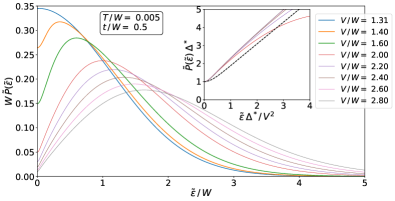
Figure 13: (Main panel) Evolution of the local field distribution in the RSB phase. The top curve corresponds to the critical coupling, $V_{c}=1.31W$. With increasing the interaction $V$, a pseudogap is formed that deepens with a slope independent of the strength of disorder $W$. (Inset) Scaling of the field distribution deep in the glassy phase.

In the main text, we have shown that the spectral function $\rho(\omega)$ displays universal scaling in the strong interaction limit. The distribution ${\widetilde{P}\,}({\widetilde{\varepsilon}\,})$ displays similar scaling properties. Similar to the SK model, ${\widetilde{P}\,}({\widetilde{\varepsilon}\,})$ scales linearly over an extended region in the limit of small quantum-tunneling and temperatures, ${\widetilde{P}\,}({\widetilde{\varepsilon}\,})\approx 1.13\;|{\widetilde{\varepsilon}\,}|/V^{2}$, with a slope independent of the strength of disorder. In the quantum limit, ${\widetilde{P}\,}(0)$ remains finite even as $T\to 0$, ${\widetilde{P}\,}(0)=1/\tilde{\Delta}$. Similar to $\rho(\omega)$, as shown in the inset of Fig. 13, $\tilde{\Delta}{\widetilde{P}\,}({\widetilde{\varepsilon}\,})$ becomes a universal function of ${\widetilde{\varepsilon}\,}\tilde{\Delta}/V^{2}$ in this quantum limit. Notice, however, that there seems to be no simple relation between the scales $\tilde{\Delta}$ and $\Delta$.