THRESHOLD SELECTION FOR EXTREMAL INDEX ESTIMATION

Abstract

We propose a new threshold selection method for the nonparametric estimation of the extremal index of stochastic processes. The so-called discrepancy method was proposed as a data-driven smoothing tool for estimation of a probability density function. Now it is modified to select a threshold parameter of an extremal index estimator. To this end, a specific normalization of the discrepancy statistic based on the Cramér-von Mises-Smirnov statistic $\omega^{2}$ is calculated by the $k$ largest order statistics instead of an entire sample. Its asymptotic distribution as $k\to\infty$ is proved to be the same as the $\omega^{2}$-distribution. The quantiles of the latter distribution are used as discrepancy values. The rate of convergence of an extremal index estimate coupled with the discrepancy method is derived. The discrepancy method is used as an automatic threshold selection for the intervals and $K-$gaps estimators and it may be applied to other estimators of the extremal index.

Keywords: Threshold selection; Discrepancy method; Cramér-von Mises-Smirnov statistic; Nonparametric estimation; Extremal index

1 Introduction

Let $X^{n}=\{X_{i}\}_{i=1}^{n}$ be a sample of random variables (r.v.s) with cumulative distribution function (cdf) $F(x)$. By Leadbetter et al. 1983 the stationary sequence $\{X_{n}\}_{n\geqslant 1}$ is said to have extremal index $\theta\in(0,1]$ if for each $0<\tau<\infty$ there is a sequence of real numbers $u_{n}=u_{n}(\tau)$ such that it holds

$$\lim_{n\to\infty}n(1-F(u_{n}))=\tau,\qquad\lim_{n\to\infty}P\{M_{n}\leqslant u_{n}\}=e^{-\tau\theta},$$

where $M_{n}=\max\{X_{1},...,X_{n}\}$. The extremal index reflects a cluster structure of an underlying sequence or its local dependence. $\theta=1$ holds if $X_{1},...,X_{n}$ are independent. For stationary sequences $\theta=1$ when mixing conditions $D(u_{n})$ and $D^{\prime}(u_{n})$ hold (Leadbetter et al. 1983).
Nonparametric estimators of $\theta$ require usually the choice of a threshold and/or a declustering parameter. The well-known blocks and runs estimators of the extremal index require an appropriate threshold $u$ and the block size $b$ or the number of consecutive observations $r$ running below $u$ to separate two clusters (Beirlant et al. 2004). A bias-corrected modification of the blocks estimator (Drees 2011) informs how to avoid the threshold selection by providing a rather stable plot of the extremal index estimates against $u$ with some remaining uncertainty. In Sun and Samorodnitsky (2018) the multilevel blocks estimator is proposed where a sequence of increasing levels and a weight function have to be defined. The sliding blocks estimator has asymptotic variance smaller than the disjoint blocks estimator (Robert et al. 2009b) and all of them require the selection of a pair $(u,b)$. The cycles estimator proposed by Ferreira (2018) needs both $u$ and the cycle size $s$ as parameters. The intervals estimator of $\theta$ by Ferro and Segers (2003) and the estimators introduced by Robert (2009b) require the choice of $u$. The $K$-gaps estimator is another threshold-based one (Süveges and Davison 2010).
One of the high quantiles of the sample $X^{n}$ is taken usually as $u$ or $u$ is selected visually corresponding to a stability interval of the plot of some estimate $\widehat{\theta}(u)$ against $u$. Following Süveges and Davison (2010), a list of pairs $(u,K)$ is selected according to the Information Matrix Test (IMT) in Fukutome et al. (2015). Then $u$ is selected from such a pair that corresponds to the largest number of clusters of exceedances separated by more than $K$ non-exceedances. The semiparametric maxima estimators (Berghaus and Bücher 2018; Northrop 2015) depend on the block size only. The choice of the latter remains an open problem.
The objective of this paper is to propose a new nonparametric tool to find the threshold $u$.
The so-called discrepancy method was proposed in Markovich (1989) and Vapnik et al. (1992) as a data-driven smoothing tool for a probability density function (pdf) estimation by i.i.d. data. We aim to extend this method for an extremal index estimation. The idea was to find an unknown parameter $h$ of the pdf as a solution of the discrepancy equation

$$\rho(\widehat{F}_{h},F_{n}) = \delta.$$

Here, $\widehat{F}_{h}(x)=\int_{-\infty}^{x}\widehat{f}_{h}(t)dt$ holds, $\hat{f}_{h}(t)$ is some pdf estimate, $\delta$ is a discrepancy value of the estimation of $F(x)$ by the empirical distribution function $F_{n}(x)$, i.e. $\delta=\rho(F,F_{n})$. $\rho(\cdot,\cdot)$ is a metric in the space of cdf’s. Since $\delta$ is usually unknown, quantiles of the limit distribution of the Cramér-von Mises-Smirnov (C-M-S) statistic

$$\omega^{2}_{n} = n\int_{-\infty}^{\infty}\left(F_{n}(x)-F(x)\right)^{2}dF(x),$$

were proposed as $\delta$. The latter limit distribution which is rather complicated can be found in Bolshev and Smirnov (1965) or Markovich (2007). One can choose other nonparametric statistics like the Kolmogorov-Smirnov or Anderson-Darling ones instead of $\omega^{2}_{n}$. Limit distributions of these statistics are invariant regarding $F(x)$ (Bolshev and Smirnov 1965). We will focus on $\omega^{2}_{n}$. Regarding practical applications the bandwidth $h$ was proposed in Markovich (1989) as a solution of the equation

$$\hat{\omega}^{2}_{n}(h)=0.05.$$ (1.1)

Here,

$$\hat{\omega}^{2}_{n}(h)=\sum_{i=1}^{n}\left(\widehat{F}_{h}(X_{i,n})-\frac{i-0.5}{n}\right)^{2}+\frac{1}{12n}$$

was calculated by the order statistics $X_{1,n}\leqslant...\leqslant X_{n,n}$ corresponding to the sample $X^{n}$, and the value $0.05$ corresponding to the mode of the pdf of the statistic $\omega^{2}_{n}$ and thus, the maximum likelihood value of the $\omega^{2}_{n}$ was found by tables of the statistic $\omega^{2}_{n}$ (Bolshev and Smirnov 1965) as the discrepancy value $\delta$. A similar idea was explored in Markovich (2015) to estimate the extremal index.
Following (Ferro and Segers 2003; Markovich 2014, 2016b, 2017) one can determine a cluster as the number of consecutive observations exceeding the threshold $u$ between two consecutive non-exceedances. Ferro and Segers (2003) state that the times between exceedances of a threshold $u$ by the process $\{X_{i}\}$, is a random variable $T(u)$ equal in distribution to $T_{1}(u)$. It holds

$$T_{1}(u) = \min\{j\geqslant 1:M_{1,j}\leqslant u,X_{j+1}>u|X_{1}>u\},$$

where $M_{i,j}=\max\{X_{i+1},...,X_{j}\}$, $M_{1,1}=-\infty$. $T_{1}(u_{n})$ normalized by the tail function $\{Y=\overline{F}(u_{n})T_{1}(u_{n})\}$, is derived to be asymptotically exponentially distributed with a weight $\theta$ and with an atom at zero with a weight $1-\theta$ (Ferro and Segers 2003).
Taking the exceedance times $1\leqslant S_{1}<...<S_{N_{u}}\leqslant n$, the observed interexceedance times are $T_{i}=S_{i+1}-S_{i}$ for $i=1,...,N_{u}-1$, where $N_{u}=\sum_{i=1}^{n}\mathbf{1}\{X_{i}>u\}$ is the number of observations which exceed a predetermined high threshold $u$ (Ferro and Segers 2003). Denote further $L\equiv L(u)=N_{u}-1$. In case of the statistic $\omega^{2}_{n}$ the discrepancy equation may be calculated by the $k$, $1\leqslant k\leqslant L$, largest order statistics of a sample $\{Y_{i}=(N_{u}/n)T_{i}\}$ as follows

$$\hat{\omega}^{2}_{L}(u)=\sum_{i=L-k+1}^{L}\left(\widehat{G}(Y_{i,L})-\frac{i-0.5}{L}\right)^{2}+\frac{1}{12L}=\delta.$$ (1.2)

Here, the distribution model of the normalized inter-exceedance times $\widehat{G}(Y_{i,L})$ is determined by $G(t)=1-\theta\exp(-\theta t)$ with a substitution of $\theta$ by some estimate $\widehat{\theta}(u)$ and of $t$ by the order statistic $Y_{i,L}$ (Markovich 2015). A value of $u$ can be found as a solution of (1.2) with regard to any consistent nonparametric estimator of $\theta$. The calculation (1.2) by the entire sample may lead to the lack of a solution of the discrepancy equation regarding $u$ the same way as for the heavy-tailed pdf estimation in (Markovich 2007; Markovich 2016a) or to too large $u$’s which may be not appropriate for the estimation of $\theta$.
The selection of $k$ and $\delta$ remains a problem. To overcome this problem we find a specific normalization of the discrepancy statistic $\hat{\omega}^{2}_{L}(u)$ in (1.2) such that its limit distribution is the same as for the C-M-S statistic. Then its quantiles may be used as $\delta$. Although the limit distribution of the C-M-S does not depend on $k$ as $k\to\infty$, for moderate samples the selection of $k$ is necessary. From Theorems 1 and 2 it is natural to select $k$ such that $k\leqslant\lfloor\theta L(u)\rfloor$. Specifically, for the discrepancy statistic the choice of $k$ has to be modified to satisfy Theorem 3. The discrepancy method can be easily applied not only to the threshold-based but generally to any extremal index estimator. In contrast to approaches based on the minimum of the mean squared error with regard to the threshold or another tuning parameter, e.g. Robert et al. (2009b), the discrepancy method does not attract any knowledge about the asymptotic rates of the variance and the bias of estimates. Similarly to Hall (1990), the minimization of the bootstrap mean squared error may require two additional parameters to select the size of a resample and to relate thresholds based on the resamples and the entire sample.
The paper is organized as follows. In Section 2 related work is recalled. In Section 3 a normalization of $\hat{\omega}^{2}_{L}(\theta)$ denoted as $\widetilde{\omega}^{2}_{L}(\theta)$ is found which has the limit distribution of $\omega^{2}_{n}$ (Theorem 2). The convergence of $\widetilde{\omega}^{2}_{L}(\widehat{\theta})$ to the $\omega^{2}_{n}$-distribution is derived when the difference $\sqrt{m_{n}}(\widehat{\theta}-\theta)$, where $m_{n}$ is some sequence relating to $k$ and $L$, has a nondegenerate distribution (Theorem 3). In Theorem 4 the consistency and the inconsistency conditions for the normalized statistic $\widetilde{\omega}^{2}_{L}(\hat{\theta})$ are given. The rate of convergence of the extremal index estimates with the threshold selected by the discrepancy method is derived in Corollary 1. The choice of the $k$ largest order statistics for $\widetilde{\omega}^{2}_{L}$ by samples of moderate sizes is discussed. Finally, an algorithm and a simulation study of the discrepancy method based on the normalized $\hat{\omega}^{2}_{L}(\widehat{\theta})$ statistic is given in Section 4 and an illustration with real data is stated in Section 5. Proofs can be found in Section 6.

2 Important mathematical results

Our results are based on Lemmas 2.2.3, 3.4.1 by de Haan and Ferreira (2006) concerning the limit distributions of the order statistics and Theorem 1 by Ferro and Segers (2003).

Lemma 1.

(de Haan and Ferreira 2006; Smirnov 1952) Let $U_{1,n}\leqslant U_{2,n}\leqslant...\leqslant U_{n,n}$ be the $n$th order statistics from a standard uniform distribution. Then, as $n\to\infty$, $k\to\infty$, $n-k\to\infty$,

$$\frac{U_{k,n}-b_{n}}{a_{n}}$$

is asymptotically standard normal with

$$b_{n}=\frac{k-1}{n-1},\qquad a_{n}=\sqrt{b_{n}(1-b_{n})\frac{1}{n-1}}.$$

Lemma 2.

(de Haan and Ferreira 2006) Let $X,X_{1},X_{2},...,X_{n}$ be i.i.d. r.v.s with common cdf $F$, and let $X_{1,n}\leqslant X_{2,n}\leqslant...\leqslant X_{n,n}$ be the $n$th order statistics. The joint distribution of $\{X_{i,n}\}^{n}_{i=n-k+1}$ given $X_{n-k,n}=t$, for some $k\in\{1,...,n-1\}$, equals the joint distribution of the set of order statistics $\{X^{*}_{i,k}\}^{k}_{i=1}$ of i.i.d. r.v.s $\{X^{*}_{i}\}^{k}_{i=1}$ with cdf

$$F_{t}(x) = P\{X\leqslant x|X>t\}=\frac{F(x)-F(t)}{1-F(t)},~{}~{}~{}x>t.$$

Definition 1.

(Ferro and Segers 2003) For real $u$ and integers $1\leqslant k\leqslant l$, let $\mathcal{F}_{k,l}(u)$ be the $\sigma$-field generated by the events $\{X_{i}>u\}$, $k\leqslant i\leqslant l$. Define the mixing coefficients $\alpha_{n,q}(u)$,

$$\alpha_{n,q}(u) = \max_{1\leqslant k\leqslant n-q}\sup|P(B|A)-P(B)|,$$

where the supremum is taken over all $A\in\mathcal{F}_{1,k}(u)$ with $P(A)>0$ and $B\in\mathcal{F}_{k+q,n}(u)$ and $k$, $q$ are positive integers.

The next theorem states that

$$\overline{F}(u_{n})T_{1}(u_{n})\to^{d}T_{\theta}=\left\{\begin{array}[]{ll}\eta,&\mbox{with probability}~{}~{}\theta,\\ 0,&\mbox{with probability}~{}~{}1-\theta,\end{array}\right.$$

where $\eta$ is exponentially distributed with mean $\theta^{-1}$. The zero asymptotic inter-exceedance times (the intracluster times) imply the times between the consecutive exceedances of the same cluster. The positive asymptotic inter-exceedance times are the inter-cluster times. $\to^{d}$ denotes convergence in distribution.

Theorem 1.

(Ferro and Segers 2003) Let $\{X_{n}\}_{n\geqslant 1}$ be a stationary process of r.v.s with tail function $\overline{F}(x)=1-F(x)$. Let the positive integers $\{r_{n}\}$ and the thresholds $\{u_{n}\}$, $n\geqslant 1$, be such that $r_{n}\to\infty$, $r_{n}\overline{F}(u_{n})\to\tau$ and $P\{M_{r_{n}}\leqslant u_{n}\}\to exp(-\theta\tau)$ hold as $n\to\infty$ for some $\tau\in(0,\infty)$ and $\theta\in(0,1]$. If there are positive integers $q_{n}=o(r_{n})$ such that $\alpha_{cr_{n},q_{n}}(u_{n})=o(1)$ for any $c>0$, then we get for $t>0$

$$P\{\overline{F}(u_{n})T_{1}(u_{n})>t\}\to\theta\exp(-\theta t),\qquad n\to\infty.$$ (2.1)

The intuition for declustering of a sample is given in Ferro and Segers (2003). One can assume that the largest $C-1=\lfloor\theta L\rfloor$ inter-exceedance times are approximately independent inter-cluster times. The larger $u$ corresponds to the larger inter-exceedance times whose number $L\equiv L(u)$ may be small. It leads to a larger variance of the estimates based on $\{T_{i}(u)\}$. The intervals estimator follows from Theorem 1. It is defined as (Beirlant et al. 2004, p. 391),

$$\hat{\theta}_{n}(u) = \Big{\{}\begin{array}[]{ll}\min(1,\hat{\theta}_{n}^{1}(u)),\mbox{ if }\max\{T_{i}:1\leqslant i\leqslant L\}\leqslant 2,\\ \min(1,\hat{\theta}_{n}^{2}(u)),\mbox{ if }\max\{T_{i}:1\leqslant i\leqslant L\}>2,\end{array}$$ (2.4)

where

$$\hat{\theta}_{n}^{1}(u)=\frac{2(\sum_{i=1}^{L}T_{i})^{2}}{L\sum_{i=1}^{L}T_{i}^{2}},~{}~{}~{}\hat{\theta}_{n}^{2}(u)=\frac{2(\sum_{i=1}^{L}(T_{i}-1))^{2}}{L\sum_{i=1}^{L}(T_{i}-1)(T_{i}-2)}.$$

The $K$-gaps estimator was proposed in Süveges and Davison (2010) as alternative to the intervals estimator, where the $K$-gaps

$$S(u_{n})^{(K)}=(\max\left(T_{1}(u_{n})-K,0\right)),~{}~{}K=0,1,2,...,$$

have the same limiting mixture law (2.1). The $K$-gaps estimator is obtained by the maximum likelihood method using the model (2.1) and assuming that the $K$-gaps observations are independent. It has the following form

$$\widehat{\theta}^{K} = 0.5\left((a+b)/c+1-\sqrt{((a+b)/c+1)^{2}-4b/c}\right),$$ (2.5)

with $a=L-N_{C}$, $b=2N_{C}$, $c=\sum_{i=1}^{L}\overline{F}(u_{n})S(u_{n})^{(K)}_{i}$. $N_{C}$ is the number of non-zero $K$-gaps. The $K$-gaps estimator is consistent and asymptotically normal as $L\to\infty$. Since the $K$-gaps may have a distribution different from (2.1) for moderate samples, $K$ is selected by a model misspecification test. The iterative weighted least squares estimator of Süveges (2007) explores the inter-exceedance times with $K=1$. The automatic selection of an optimal pair $(u,K)$ is proposed in Fukutome et al. (2015) by a choice of pairs for which values of the statistic of the information matrix test (the IMT) are less than $0.05$. The test works satisfactorily when the number of exceedances is not less than $80$.
The intervals estimator is derived to be consistent for $m$-dependent processes (Ferro and Segers 2003). Asymptotic normality $\sqrt{m_{n}}(\hat{\theta}_{n}(u)-\theta)\to^{d}N(0,V)$ as $n\to\infty$ is derived for several extremal index estimators and different values of variance $V$. Here, $m_{n}=np_{n}$ holds for the blocks and runs estimators, where $p_{n}=\mathrm{P}\{X_{1}>u_{n}\}$ holds in Weissman and Novak (1978); $m_{n}=L(u_{n})$ is the number of inter-exceedance times $\{T_{i}(u_{n})\}$ for the intervals estimator in Robert (2009a), $\lfloor x\rfloor$ denotes the integer part of $x$; $m_{n}=n/p_{n}$ is taken for the multilevel blocks estimator in Sun and Samorodnitsky (2018), where $p_{n}\overline{F}(u_{n}^{s})\to\tau_{s}$ and $s\in\{1,...,m\}$ is the number of levels $\{u_{n}^{s}\}$; $m_{n}=\lfloor n/r_{n}\rfloor$ is used for the disjoint and sliding blocks estimators, where $r_{n}=o(n)$ are positive integers related to a mixing condition (Robert 2009a); $m_{n}=k_{n}$ is taken for the disjoint and sliding blocks estimators by Berghaus and Bücher (2018) and Northrop (2015), where $k_{n}$ is a number of blocks of length $b_{n}$ such that $k_{n}=o(b^{2}_{n})$ holds as $n\to\infty$.

3 Main results: $\omega^{2}$-distribution of the normalized Cramér-von Mises-Smirnov statistic

3.1 Normalized Cramér-von Mises-Smirnov statistic for known $\theta$

Let us rewrite the left-hand side (1.2) in the following form

$$\hat{\omega}^{2}_{L}(u)=\sum_{i=L-k+1}^{L}\left(1-\theta\exp(-Y_{i,L}\theta)-\frac{i-0.5}{L}\right)^{2}+\frac{1}{12L}$$ (3.1)

and derive its limit distribution. Note that $L=L(u_{r_{n}})$ is a sequence of r.v.s converging in probability to infinity due to (Theorem 2.1, Robert 2009a). In sequel, the limit distribution of the concerned statistics does not depend on $L$, so we can neglect its randomness. The threshold sequence $u_{r_{n}}$ introduced in Robert (2009a) corresponds to the point process of time normalized exceedances defined on $(0,\infty)$, in contrast to a traditional point process defined on $(0,1)$ (Beirlant et al. 2004).
According to (Martynov 1978; Smirnov 1952) the limit distribution of the C-M-S statistic (1) or of $\omega^{2}_{n}=n\int_{0}^{1}\left(F_{n}(t)-t\right)^{2}dt$ coincides with the distribution of

$$\Omega = \int_{0}^{1}B^{2}(t)dt,$$

where $B(t)$ is a Brownian bridge on $[0,1],$ i.e. the Gaussian random process with zero mean and the covariance function $R(s,t)=\min(s,t)-st,$ $s,t\in[0,1]$. Then the statistic (3.1) built by the $k$ largest order statistics tends to $0$ for $k=o(L)$ as $L\to\infty$, since the interval over which we integrate $B^{2}(t)$ tends to an empty set. Thus, (3.1) has to be normalized. Let us consider the normalization of (3.1)

$$\widetilde{\omega}^{2}_{L}(\theta)=\frac{1}{(1-t_{k})^{2}}\cdot$$

$$\cdot \sum\limits_{i=L-k+1}^{L}\left(1-\theta\exp(-Y_{i,L}\theta)-t_{k}-\frac{i-(L-k)-0.5}{k}(1-t_{k})\right)^{2}+\frac{1}{12k},$$

where $t_{k}=1-\theta\exp(-Y_{L-k,L}\theta)$. Let us explain in more detail why we need such normalization. It follows from (Robert 2009a, Theorem 2.1), that there are a probability, $\theta$, of asymptotic positive inter-exceedance times (the inter-cluster times) and a probability, $1-\theta,$ of zero asymptotic inter-exceedance times (the intra-cluster times). Moreover, the inter-cluster times are asymptotically independent exponential with mean $1/\theta$. Let us consider the following statistic

$$\omega^{2}_{k}(\theta)=\frac{1}{Z_{L-k,L}^{2}}\cdot$$ (3.3)

$$\cdot \sum\limits_{i=L-k+1}^{L}\left(Z_{L-k,L}-Z_{i,L}-\frac{i-(L-k)-0.5}{k}Z_{L-k,L}\right)^{2}+\frac{1}{12k},$$

where $Z_{i,L}=\theta\exp(-T^{*}_{i,L}\theta)$, $T^{*}_{1,L}\leqslant\ldots\leqslant T^{*}_{L,L}$ are order statistics of a sample $\{T^{*}_{i}\},$ $\{T^{*}_{i}\}$ are independent copies of $T_{\theta}$.

It follows from (3.3), Theorem 1 and Lemma 2, that the conditional distribution of the set of order statistics $\{1-Z_{i,L}\}_{i=L-k+1}^{L}$ given $1-Z_{L-k,L}=t_{k}$ asymptotically agrees for $\limsup_{n\to\infty}k/L<\theta$ with the distribution of the set of order statistics $\{U^{\ast}_{j,k}\},$ $j=i-(L-k),$ of an i.i.d. sample $\{U_{j}^{\ast}\}$ from the uniform distribution on $[t_{k},1]$. The asymptotical distribution of $\omega^{2}_{k}(\theta)$ is given in the next theorem.

Theorem 2.

It holds

$$\omega^{2}_{k}(\theta)\stackrel{{\scriptstyle d}}{{\to}}\xi$$

as $k\to\infty$, $L\to\infty$, $\limsup_{n\to\infty}k/L<\theta$, where $\xi$ has the distribution function $A_{1},$ which is the limit distribution function of the C-M-S statistic $\omega^{2}_{n}$.

Remark 1.

Based on the proof of Theorem 2, one can propose the goodness-of-fit test of von Mises’ type to check the hypothesis $H_{0}:F(x)=F_{0}(x)$ for sufficiently large $x$ using the largest order statistics of a sample $\{X_{i}\}_{i=1}^{n}.$ The test statistic is the following

$$\omega^{2}_{k}=\sum_{i=0}^{k-1}\left(\frac{F_{0}(X_{n-i,n})-F_{0}(X_{n-k,n})}{1-F_{0}(X_{n-k,n})}-\frac{k-i-0.5}{k}\right)^{2}+\frac{1}{12k}.$$

Theorem 2 implies, that the limit distribution of the statistic $\omega^{2}_{k}$ under the hypothesis $H_{0}$ does not depend on $k$ and $n$. It is equal to the limit distribution of the C-M-S statistic, if the hypothesis $H_{0}$ is true. The consistency of the proposed test follows from the equality in distribution of the test statistic given $F_{0}(X_{n-k,n})=t$ and the C-M-S statistic. The test is based on the largest order statistics of a sample. It is reasonable both if only the upper tail of the distribution is of interest and/or if the largest order statistics of a sample are only available.

3.2 Normalized Cramér-von Mises-Smirnov statistic for unknown $\theta$

Here, we check whether one can substitute $\theta$ by its estimate $\widehat{\theta}$ in (3.1) and find conditions imposed on $\widehat{\theta}$ under which the limit distribution of $\widetilde{\omega}^{2}_{L}(\theta)$ will be the same as the limit distribution of $\omega^{2}_{k}(\theta).$ Recall again that the number of inter-exceedance times $L=L(u_{r_{n}})$ is a sequence of r.v.s tending to $+\infty$ (Robert 2009a). It follows from Theorem 2 that the limit distribution of $\omega^{2}_{k}(\theta)$ does not depend on $L(u_{r_{n}})$. We can assume that $L(u_{r_{n}})$ is a numerical sequence tending to infinity as $n\to\infty.$ We will write $L$ instead of $L(u_{r_{n}})$ in the sequel.

In spirit of Theorem 3.2 (Robert 2009a), the limit distribution of the following statistic

$$\sqrt{L}\left(\sum_{i=1}^{L-1}f(Y_{i})-Ef(Y_{1})\right)$$

for some continuous $f$ may not depend on a substitution of the set of r.v.s $\{T^{*}_{i}\}_{i=1}^{L-1}$ appearing in (3.3) instead of $\{Y_{i}\}_{i=1}^{L-1}.$ Moreover, $T^{*}_{i}\stackrel{{\scriptstyle d}}{{=}}T_{\theta},$ $i\in\{1,\ldots,L-1\}$ and there is a probability $\theta$ of the nonzero elements of this set that are independent exponentially distributed with parameter $\theta$. For convenience, we accept further $L$ instead of $L-1$. For these r.v.s, Theorem 2.2.1 (de Haan and Ferreira 2006) implies that if $k/L\to 0$ and $k\to\infty$ as $L\to\infty,$ then

$$\sqrt{k}(T^{*}_{L-k,L}-\ln(L\theta/k)/\theta)=O_{P}(1).$$

In light of these remarks let us assume that there exists a sample of independent exponentially distributed r.v.s $\{E_{i}^{(L)}\}_{i=1}^{l}$ with mean $\theta^{-1}$ for all large enough $L$ such that

$$Y_{L-k,L}-E_{l-k,l}^{(L)}=o_{P}\left(\frac{1}{\sqrt{k}}\right)$$ (3.4)

if $k/L\to 0$ and $k\to\infty$ as $L\to\infty$, where we denote $l=\lfloor\theta L\rfloor$ and assume $k<l$. Here and further, we denote for brevity a sequence of positive integers $\{k_{n}\}$ as $k$. Theorem 2 remains valid when $T^{*}_{i,L}$, $i\in\{L-k,...,L\}$ in $\omega_{k}^{2}(\theta)$ are substituted by $E^{(L)}_{i,l}$, $i\in\{l-k,...,l\}$.

Theorem 3.

Let the conditions of Theorem 1 and the condition (3.4) be fulfilled and the estimator of the extremal index $\widehat{\theta}=\widehat{\theta}_{n}$ be such that

$$\sqrt{m_{n}}(\widehat{\theta}_{n}-\theta)\stackrel{{\scriptstyle d}}{{\to}}\zeta,~{}~{}n\to\infty,$$ (3.5)

where the r.v. $\zeta$ has a nondegenerate distribution function $H$. Let us assume that the sequence $m_{n}$ is such that

$$\frac{k}{m_{n}}=o(1)\ \mbox{ and }\ \frac{(\ln L)^{2}}{m_{n}}=o(1)$$ (3.6)

as $n\to\infty$. Then

$$\widetilde{\omega}^{2}_{L}(\widehat{\theta}_{n}) \stackrel{{\scriptstyle d}}{{\to}} \xi\sim A_{1}$$

holds, where $A_{1}$ is the limit distribution function of the C-M-S statistic.

Remark 2.

Normal distributions give examples of $H$ regarding the intervals, blocks and sliding blocks estimators of the extremal index (Northrop 2015; Robert 2009a; Robert et al. 2009; Sun and Samorodnitsky 2018).

Remark 3.

The replacement of $o(1)$ by $O(1)$ in (3.6) violates Theorem 3. The assumption $k=O(m_{n})$ may lead to a limit distribution of $\widetilde{\omega}^{2}_{L}(\widehat{\theta}_{n})$ different from $A_{1}$ that is out of scope of the paper.

Remark 4.

The limit process of the point process of exceedance times is a compound Poisson process (Hsing et al. 1988). The condition (3.4) shows in fact the rate of this convergence required for the limit distribution of the normalized C-M-S statistic that is built by the largest $k$ order statistic to preserve the limit distribution of $\omega^{2}$.

Theorem 4.

Let the conditions of Theorem 1 and (3.4) be fulfilled. Assume that the sequence of estimates $\{\hat{\theta}_{n}\}$ is such that for some $\alpha\in[0,1/2]$

$$k_{n_{s}}^{\alpha}|\hat{\theta}_{n_{s}}-\theta|\stackrel{{\scriptstyle P}}{{\rightarrow}}+\infty,\qquad\mbox{if}\qquad 0<\alpha\leqslant 1/2,$$

$$|\hat{\theta}_{n_{s}}-\theta|>\varepsilon\qquad\mbox{for some}\qquad\varepsilon>0,\qquad\mbox{if}\qquad\alpha=0$$

hold as $n\to\infty$ for some subsequence $\{k_{n_{s}}\},$ $s\geqslant 1,$ of the sequence $\{k_{n}\}$. Then for corresponding subsequence $\{L_{s}\}$ of the sequence $\{L\}$

$$\widetilde{\omega}^{2}_{L_{s}}(\hat{\theta}_{n_{s}})/k_{n_{s}}^{1-2\alpha}\stackrel{{\scriptstyle P}}{{\rightarrow}}+\infty$$

holds as $n\to\infty.$

Remark 5.

Theorem 4 implies that the non-consistency of the estimator $\widehat{\theta}_{n}$ or the consistency with a sufficiently slow rate leads to the non-consistency of $\widetilde{\omega}^{2}_{L_{s}}(\widehat{\theta}_{n})$ in a sense that its limit distribution does not exist or the latter statistic tends to $+\infty$. In case that $\alpha\neq 0$ holds, the estimator $\widehat{\theta}_{n}$ may be consistent but with the rate of convergence slower than $k_{n}^{-\alpha}$. Hence, $\widetilde{\omega}^{2}_{L}(\widehat{\theta}_{n})$ may be considered as a quality functional of $\widehat{\theta}_{n}$.

The consistency of the corresponding extremal index estimates follows from Theorem 4. The next corollary states, if the solutions of the discrepancy equation exist for each $n$, then the consistency is fulfilled.

Corollary 1.

Let $\hat{\theta}_{n}(u_{n})$ be an estimator of $\theta$ and $\{\tilde{u}_{k,L}\}$ be some sequence of solutions of the discrepancy equation. Then $\hat{\theta}_{n}(\tilde{u}_{k,L})\stackrel{{\scriptstyle P}}{{\rightarrow}}\theta$ and for arbitrary $\varepsilon>0$

$$k^{1/2-\varepsilon}|\hat{\theta}_{n}(\tilde{u}_{k,L})-\theta|\stackrel{{\scriptstyle P}}{{\rightarrow}}0$$

hold as $k\to\infty,$ $L/k\to\infty,$ $L=o(n)$, $n\to\infty.$

The proof of the corollary is based on a negation of the assertion of Theorem 4.

3.3 The choice of $k$

According to Theorem 3 the asymptotic distribution of $\widetilde{\omega}^{2}_{L}(\widehat{\theta}_{n})$ does not depend on $k$. The $k$-selection gives another viewpoint that using only the largest inter-exceedance times screens out the smallest inter-exceedance times. It is helpful for the reasons discussed in Ferro and Segers (2003) and is the motivation for the introduction of the tuning parameter $K$ in the $K-$gaps estimator of $\theta$ proposed in Süveges and Davison (2010).
In practice, for each predetermined $\delta$, $u$ and $L(u)$ one may decrease the $k$-value such that $k\leqslant\min\{\widehat{\theta}_{0}L(u),L(u)^{\beta}\}$, $0<\beta<1$, ($\widehat{\theta}_{0}$ is some pilot estimate of $\theta$) until the discrepancy equations have solutions and select the largest one among such $k$’s. This choice satisfies Theorem 3 but it is not unique. For instance, one can select $k=\lfloor(\ln L)^{2}\rfloor)$. The following simulation shows an ideal case when the accuracy is the best. Namely, the $K-$gaps estimator with $K=0$ and $N_{C}=k$ coupled with the discrepancy method demonstrates the best choice when $k=\lfloor\theta L\rfloor$ is chosen. Since $\theta$ is in reality unknown, one has to take $k=\lfloor\widehat{\theta}_{0}L\rfloor$. This choice requires an accurate consistent pilot estimate $\widehat{\theta}_{0}$.

4 Simulation study

In our simulation study we focus on the threshold-based intervals and $K-$gaps estimators. We propose also a modification of the $K-$gaps estimator with $K=0$ and $N_{C}=k$ in (2.5) notated as $\widehat{\theta}^{K_{0}}$. The latter coupled with the discrepancy method demonstrates the best accuracy if an estimate $\widehat{\theta}_{0}$ is close to $\theta$. The natural drawback of the intervals estimator is that it needs a large sample size $n$ to obtain a moderate size $L(u)$ for a large $u$. The same concerns the $K$-gaps estimator.

Algorithm 1.

1. Using $X^{n}=\{X_{i}\}_{i=1}^{n}$ and taking thresholds $u$ corresponding to quantile levels $q\in\{0.90,0.905,...,0.995\}$, generate samples of the inter-exceedance times $\{T_{i}(u)\}$ and the normalized r.v.s

   $$\{Y_{i}\}=\{\overline{F}(u)T_{i}(u)\}=\{(N_{u}/n)T_{i}(u)\},~{}i\in\{1,2,...,L\},~{}L=L(u),$$ (4.1)

   where $N_{u}$ is the number of exceedances over threshold $u$.

2. For each $u$ select $k=\lfloor\widehat{\theta}_{0}L\rfloor$, $k=\min\{\lfloor\widehat{\theta}_{0}L\rfloor,\sqrt{L}\}$ (in case $\widehat{\theta}_{0}=1$, accept $k=L-1$) or $k=\lfloor(\ln L)^{2}\rfloor$, where the intervals estimator (2.4) may be selected as a pilot estimator $\widehat{\theta}_{0}=\widehat{\theta}_{0}(u)$ with the same $u$ as in Item 1.

3. Use a sorted sample $Y_{L-k+1,L}\leqslant...\leqslant Y_{L,L}$ and find among considered quantiles all solutions $u_{1},...,u_{l}$ (here, $l$ is a random number) of the following discrepancy equation

   $$\!\!\!\!\!\!\widetilde{\omega}^{2}_{L}(\widehat{\theta})=\frac{1}{(1-\widehat{t}_{k})^{2}}\cdot$$ (4.2)

   $$\!\!\!\!\!\!\!\!\!\!\sum\limits_{i=L-k+1}^{L}\left(1-\widehat{\theta}\exp(-Y_{i,L}\widehat{\theta})-\widehat{t}_{k}-\frac{i-(L-k)-0.5}{k}(1-\widehat{t}_{k})\right)^{2}+\frac{1}{12k}=\delta_{1},$$

   where $\widehat{t}_{k}=1-\widehat{\theta}\exp(-Y_{L-k,L}\widehat{\theta})$, $\widehat{\theta}=\widehat{\theta}(u)$ is calculated by (2.4), and $\delta_{1}=0.05$ is the mode of the C-M-S statistic. If $L<40$ we should replace $\widetilde{\omega}^{2}_{L}(\widehat{\theta})$ by

   $$(\widetilde{\omega}^{2}_{L}(\widehat{\theta}))^{\prime}=\left(\widetilde{\omega}^{2}_{L}(\widehat{\theta})-\frac{0.4}{L}+\frac{0.6}{L^{2}}\right)\left(1+\frac{1}{L}\right)$$

   and use quantiles of the C-M-S statistic as the discrepancy $\delta$ (Kobzar 2006).

4. For each $u_{j}$, $j\in\{1,...,l\}$ calculate $\hat{\theta}(u_{j})$ and find

   $$\widehat{\theta}_{1}=\frac{1}{l}\sum_{i=1}^{l}\widehat{\theta}(u_{i}),~{}\widehat{\theta}_{2}=\widehat{\theta}(u_{min}),~{}\widehat{\theta}_{3}=\widehat{\theta}(u_{max})$$ (4.3)

   as resulting estimates, where $u_{min}=\min\{u_{1},...,u_{l}\}$, $u_{max}=\max\{u_{1},...,u_{l}\}$.

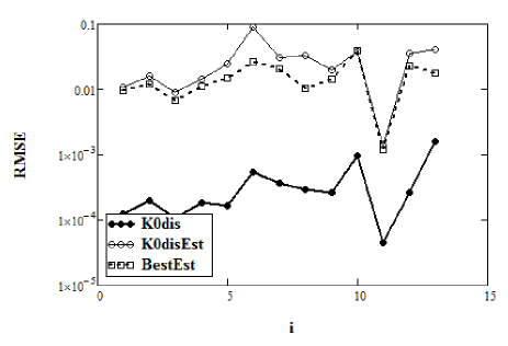
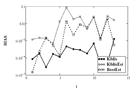
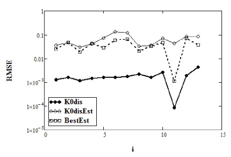
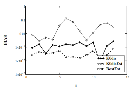
Figure 1: The best RMSE and Bias for the K-gaps estimator $\widehat{\theta}^{K_{0}}$ with the threshold $u$ selected by the discrepancy equation (4.2) and the corresponding inequality (4.4) and with $k=\lfloor sL\rfloor$, where ’K0dis’ and ’K0disEst’ correspond to $s=\theta$ and $s=\widehat{\theta}_{0}$ in Tables 1 and 2, respectively, $\widehat{\theta}_{0}$ is a pilot intervals estimate; the best RMSE and Bias among all estimates in Tables 3-8 notated as ’BestEst’ against the number of processes related to the column labels in Tables 1-8, and enumerated from left to right as in the tables for sample size $n=10^{5}$ (the upper row) and $n=5000$ (the lower row).

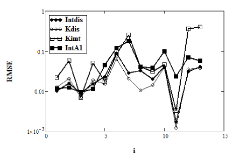
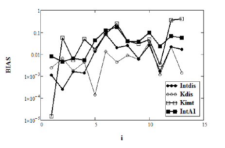
Figure 2: The best RMSE and Bias for the intervals estimator (’Intdis’) and K-gaps (’Kdis’) estimators with threshold $u$ selected by the discrepancy equation (4.2) and the corresponding inequality (4.4), and for the K-gaps estimator with $u$ selected by the test IMT (’Kimt’) and the intervals estimator with the ”plateau-finding” algorithm A1 to select $u$ (’IntA1’) against the number of processes related to the column labels in Tables 3 and 4, and enumerated from left to right as in the tables for sample size $n=10^{5}$.

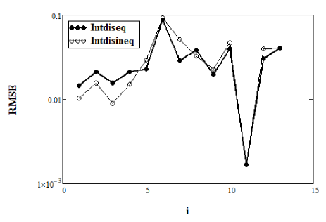
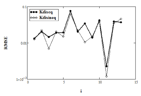
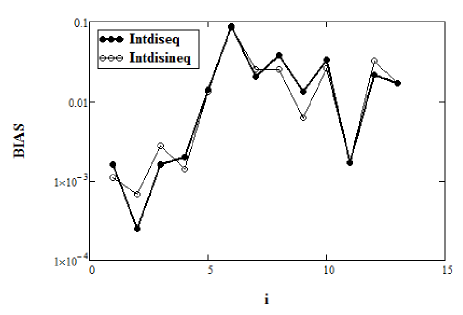
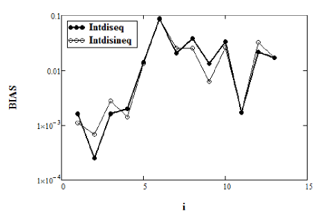
Figure 3: The best RMSE and Bias for the intervals estimator (left column) and K-gaps estimator (right column) obtained by the Algorithm with (4.2) notated as ’Intdiseq’ and ’Kdiseq’, and with the inequality (4.4) notated as ’Intdisineq’ and ’Kdisineq’ against the number of processes related to the column labels in Tables 3 and 4 for sample size $n=10^{5}$.

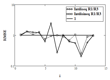
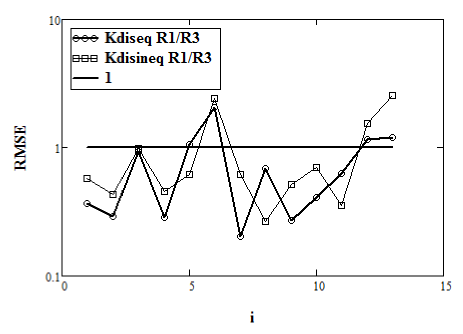
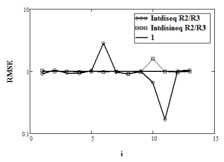
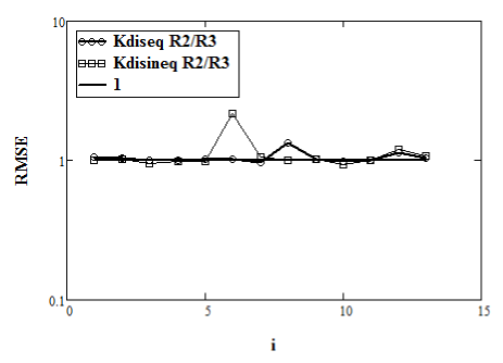
Figure 4: Ratios $R1/R3$ and $R2/R3$ of the best RMSE for the intervals estimator (left column) and K-gaps estimator (right column) obtained by the Algorithm with the equation (4.2) notated as ’Intdiseq’ and ’Kdiseq’, and with the inequality (4.4) notated as ’Intdisineq’ and ’Kdisineq’ against the number of processes related to the column labels in Tables 3, 5 and 7: The $R1/R3$ corresponds to the best results in Table 3 divided to those in Table 7, and the $R2/R3$ - to those in Tables 5 and 7, respectively, for sample size $n=10^{5}$.

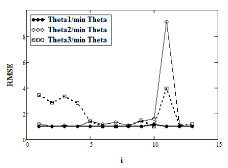
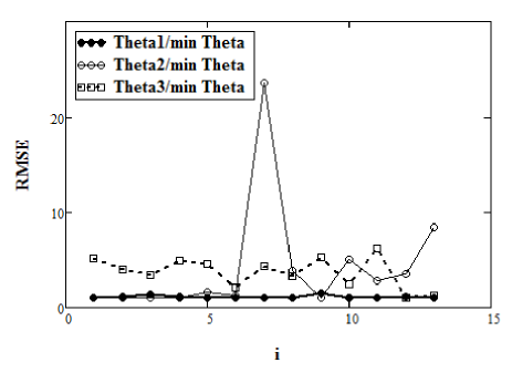
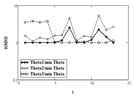
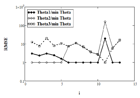
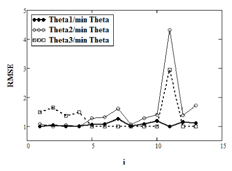
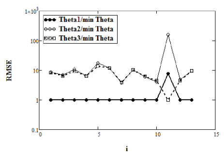
Figure 5: Ratios of the RMSEs $RMSE(\widehat{\theta}_{i})/\min_{i}(RMSE(\widehat{\theta}_{i}))$ corresponding to estimates $\{\widehat{\theta}_{i}\}$, $i\in\{1,2,3\}$ in (4.3) for the intervals estimator (left column) and the K-gaps estimator (right column) obtained by the Algorithm with (4.4) against the number of processes related to the column labels in Tables 3, 5 and 7: The upper figures correspond to $k=\lfloor\widehat{\theta}_{0}L\rfloor$ in Table 3, the middle figures to $k=\lfloor\min(\widehat{\theta}_{0}L,\sqrt{L})\rfloor$ in Table 5 and the lower figures to $k=\lfloor(\ln L)^{2}\rfloor$ in Table 7, for sample size $n=10^{5}$.

Table 1: The root mean squared error of $\widehat{\theta}^{K_{0}}$ ($k=\lfloor sL\rfloor$), $\widehat{\theta}_{0}$ is a pilot intervals estimate.

$RMSE$	MM		ARMAX		$ARu^{+}$		$ARu^{-}$		$MA(2)$		ARc	AR(2)	GARCH
$\cdot 10^{4}$/$\theta$	$0.5$	$0.8$	$0.25$	$0.75$	$0.5$	$0.8$	$0.75$	$0.96$	$0.5$	$2/3$	$0.3$	$0.25$	$0.447$
$n=10^{5}$
$s=\theta$
$\widehat{\theta}^{K0dis}_{1}$	9.018	11	8.879	10	9.489	19	15	19	12	10	5.709	9.104	16
$\widehat{\theta}^{K0dis}_{2}$	8.701	11	8.741	9.985	9.042	19	14	19	12	10	5.709	9.081	16
$\widehat{\theta}^{K0dis}_{3}$	9.866	12	9.264	11	10	19	15	19	12	10	5.709	9.141	16
$\widehat{\theta}^{K0dis*}_{1}$	3.419	5.357	2.438	5.016	4.292	9.341	7.617	7.434	5.507	9.527	0.605	4.696	19
$\widehat{\theta}^{K0dis*}_{2}$	1.244	1.959	1.073	1.859	1.681	5.412	3.712	2.938	2.643	9.569	0.446	2.667	17
$\widehat{\theta}^{K0dis*}_{3}$	14	17	14	16	14	16	16	19	14	10	5.709	11	22
$s=\widehat{\theta}_{0}$
$\widehat{\theta}^{K0dis}_{1}$	161	213	154	196	251	893	304	386	196	376	-	357	-
$\widehat{\theta}^{K0dis}_{2}$	159	213	150	195	249	894	304	387	198	377	-	357	-
$\widehat{\theta}^{K0dis}_{3}$	168	216	165	202	256	893	303	386	196	376	-	357	-
$\widehat{\theta}^{K0dis*}_{1}$	106	159	89	150	299	931	525	329	229	540	14	401	413
$\widehat{\theta}^{K0dis*}_{2}$	126	157	103	145	415	1072	690	361	324	734	156	424	404
$\widehat{\theta}^{K0dis*}_{3}$	348	443	293	445	419	989	511	350	335	463	86	446	474
$n=5000$
$s=\theta$
$\widehat{\theta}^{K0dis}_{1}$	152	147	138	151	162	189	199	211	173	254	-	199	106
$\widehat{\theta}^{K0dis}_{2}$	134	134	125	133	146	177	186	191	155	244	-	186	106
$\widehat{\theta}^{K0dis}_{3}$	214	180	181	202	207	210	232	251	216	274	-	231	109
$\widehat{\theta}^{K0dis*}_{1}$	60	59	59	51	61	60	63	79	65	82	65	66	85
$\widehat{\theta}^{K0dis*}_{2}$	13	16	12	15	16	16	18	22	16	27	0.87683	19	44
$\widehat{\theta}^{K0dis*}_{3}$	441	334	480	423	446	323	417	400	447	428	815	437	236
$s=\widehat{\theta}_{0}$
$\widehat{\theta}^{K0dis}_{1}$	1035	608	579	900	799	1444	1275	391	603	886	-	1143	1621
$\widehat{\theta}^{K0dis}_{2}$	1003	589	562	867	779	1398	1235	393	607	908	-	1137	1625
$\widehat{\theta}^{K0dis}_{3}$	1117	707	690	1006	881	1503	1301	392	672	928	-	1160	1622
$\widehat{\theta}^{K0dis*}_{1}$	359	484	366	469	732	1310	1360	324	352	712	550	949	981
$\widehat{\theta}^{K0dis*}_{2}$	362	466	299	411	803	1606	1708	395	574	1174	422	848	851
$\widehat{\theta}^{K0dis*}_{3}$	1765	1573	1578	1729	2004	1722	1843	679	1684	1725	2242	1833	2183

Table 2: The absolute bias of $\widehat{\theta}^{K_{0}}$ ($k=\lfloor sL\rfloor$), $\widehat{\theta}_{0}$ is a pilot intervals estimate.

$|Bias|$	MM		ARMAX		$ARu^{+}$		$ARu^{-}$		$MA(2)$		ARc	AR(2)	GARCH
$\cdot 10^{4}$/$\theta$	$0.5$	$0.8$	$0.25$	$0.75$	$0.5$	$0.8$	$0.75$	$0.96$	$0.5$	$2/3$	$0.3$	$0.25$	$0.447$
$n=10^{5}$
$s=\theta$
$\widehat{\theta}^{K0dis}_{1}$	5.824	10	2.935	9.194	6.493	19	13	19	8.306	6.956	5.709	1.425	16
$\widehat{\theta}^{K0dis}_{2}$	5.427	9.432	2.818	8.703	6.086	19	13	19	8.065	6.956	5.709	1.470	16
$\widehat{\theta}^{K0dis}_{3}$	6.299	11	3.041	9.727	6.899	19	14	19	8.547	6.956	5.709	1.381	16
$\widehat{\theta}^{K0dis*}_{1}$	2.789	5.198	1.167	4.799	3.495	8.924	7.232	7.409	4.402	8.053	0.605	1.284	16
$\widehat{\theta}^{K0dis*}_{2}$	0.859	1.851	0.298	1.708	1.161	4.739	3.280	2.914	1.876	8.286	0.446	0.519	13
$\widehat{\theta}^{K0dis*}_{3}$	9.880	16	5.288	15	10	15	15	19	10	7.017	5.709	2.693	20
$s=\widehat{\theta}_{0}$
$\widehat{\theta}^{K0dis}_{1}$	16	19	18	41	135	876	182	382	125	313	-	276	-
$\widehat{\theta}^{K0dis}_{2}$	12	15	14	37	137	878	183	383	127	315	-	276	-
$\widehat{\theta}^{K0dis}_{3}$	18	23	23	44	134	875	182	382	123	312	-	276	-
$\widehat{\theta}^{K0dis*}_{1}$	28	15	28	7.082	268	919	481	315	200	510	14	357	177
$\widehat{\theta}^{K0dis*}_{2}$	76	38	76	52	402	1065	668	348	302	707	156	393	193
$\widehat{\theta}^{K0dis*}_{3}$	57	65	46	72	157	889	293	259	49	246	86	318	161
$n=5000$
$s=\theta$
$\widehat{\theta}^{K0dis}_{1}$	101	117	76	98	112	162	138	182	119	192	-	125	12
$\widehat{\theta}^{K0dis}_{2}$	75	97	57	74	91	145	118	153	97	176	-	105	13
$\widehat{\theta}^{K0dis}_{3}$	142	145	104	128	141	182	162	217	147	207	-	148	11
$\widehat{\theta}^{K0dis*}_{1}$	56	58	51	49	57	59	60	79	61	78	65	56	58
$\widehat{\theta}^{K0dis*}_{2}$	8.9597	16	3.3883	14	11	16	14	22	12	22	0.87683	12	27
$\widehat{\theta}^{K0dis*}_{3}$	405	326	410	413	409	316	407	400	412	410	815	372	102
$s=\widehat{\theta}_{0}$
$\widehat{\theta}^{K0dis}_{1}$	436	202	149	332	384	1312	750	370	84	163	-	601	328
$\widehat{\theta}^{K0dis}_{2}$	365	161	111	276	370	1255	720	370	31	219	-	577	319
$\widehat{\theta}^{K0dis}_{3}$	505	243	203	400	404	1355	782	371	143	110	-	625	337
$\widehat{\theta}^{K0dis*}_{1}$	119	168	124	153	576	1252	1236	279	153	571	550	777	410
$\widehat{\theta}^{K0dis*}_{2}$	81	29	49	37	684	1557	1619	386	466	1092	422	688	386
$\widehat{\theta}^{K0dis*}_{3}$	1015	810	946	1053	1184	1421	1143	152	946	810	2242	1256	1086

Table 3: The root mean squared error ($k=\lfloor\widehat{\theta}_{0}L\rfloor$), $\widehat{\theta}_{0}$ is a pilot intervals estimate.

$RMSE$	MM		ARMAX		$ARu^{+}$		$ARu^{-}$		$MA(2)$		ARc	AR(2)	GARCH
$\cdot 10^{4}$/$\theta$	$0.5$	$0.8$	$0.25$	$0.75$	$0.5$	$0.8$	$0.75$	$0.96$	$0.5$	$2/3$	$0.3$	$0.25$	$0.447$
$n=10^{5}$
$\widehat{\theta}_{1}$	147	215	159	211	230	887	287	383	199	400	-	305	-
$\widehat{\theta}_{2}$	146	213	158	211	230	889	287	384	201	402	-	305	-
$\widehat{\theta}_{3}$	154	222	164	215	235	886	287	383	203	400	-	305	-
$\widehat{\theta}_{1}^{*}$	103	160	89	151	292	928	516	328	229	542	17	400	413
$\widehat{\theta}_{2}^{*}$	123	156	99	151	410	1070	690	354	324	745	155	420	405
$\widehat{\theta}_{3}^{*}$	354	442	294	425	413	957	516	351	336	467	67	443	470
$\widehat{\theta}^{Kdis}_{1}$	133	204	145	190	195	772	209	349	141	423	-	390	375
$\widehat{\theta}^{Kdis}_{2}$	777	844	648	940	799	777	208	1396	799	420	-	519	382
$\widehat{\theta}^{Kdis}_{3}$	895	702	651	821	398	763	207	1115	927	637	-	477	389
$\widehat{\theta}^{Kdis*}_{1}$	136	264	100	237	150	631	220	105	229	390	12	394	464
$\widehat{\theta}^{Kdis*}_{2}$	127	226	70	207	249	788	5189	404	152	1944	34	1231	3929
$\widehat{\theta}^{Kdis*}_{3}$	652	897	238	1013	690	1300	963	345	798	958	75	353	573
$\widehat{\theta}^{Kimt}$	217	569	69	498	173	844	2501	401	309	466	33	3630	4028
$\widehat{\theta}^{IA1}$	116	122	95	113	447	1193	1756	399	387	977	233	693	580
$n=5000$
$\widehat{\theta}_{1}$	565	938	506	818	783	1431	1364	394	533	816	-	900	1497
$\widehat{\theta}_{2}$	557	913	476	787	748	1401	1337	396	537	810	-	897	1497
$\widehat{\theta}_{3}$	633	1013	620	903	879	1490	1416	394	593	850	-	910	1497
$\widehat{\theta}_{1}^{*}$	359	496	350	464	715	1294	1276	315	352	760	606	835	955
$\widehat{\theta}_{2}^{*}$	352	466	291	450	808	1587	1666	395	557	1179	422	794	870
$\widehat{\theta}_{3}^{*}$	1635	1564	1377	1652	1902	1644	1754	713	1505	1656	1455	1610	2036
$\widehat{\theta}^{Kdis}_{1}$	480	917	496	772	787	1186	1820	427	406	807	-	1690	1877
$\widehat{\theta}^{Kdis}_{2}$	1525	1880	982	1793	1836	1863	2672	2981	1218	2020	-	1855	2929
$\widehat{\theta}^{Kdis}_{3}$	1624	1993	1286	1815	1692	1686	2348	1775	1924	2349	-	1737	2337
$\widehat{\theta}^{Kdis*}_{1}$	320	605	299	507	453	592	641	213	404	754	72	1528	1491
$\widehat{\theta}^{Kdis*}_{2}$	252	548	199	487	535	866	2529	423	335	488	25	3684	3787
$\widehat{\theta}^{Kdis*}_{3}$	824	1007	931	871	1086	927	916	555	714	929	2321	1106	1324
$\widehat{\theta}^{Kimt}$	247	588	188	525	293	869	2518	418	325	474	25	3680	3900
$\widehat{\theta}^{IA1}$	385	513	319	478	694	1388	1985	394	514	1114	676	980	1077

Table 4: The absolute bias ($k=\lfloor\widehat{\theta}_{0}L\rfloor$), $\widehat{\theta}_{0}$ is a pilot intervals estimate.

$|Bias|$	MM		ARMAX		$ARu^{+}$		$ARu^{-}$		$MA(2)$		ARc	AR(2)	GARCH
$\cdot 10^{4}$/$\theta$	$0.5$	$0.8$	$0.25$	$0.75$	$0.5$	$0.8$	$0.75$	$0.96$	$0.5$	$2/3$	$0.3$	$0.25$	$0.447$
$n=10^{5}$
$\widehat{\theta}_{1}$	18	2.515	20	21	142	872	203	380	132	333	-	217	-
$\widehat{\theta}_{2}$	16	2.498	16	20	142	874	203	381	134	335	-	217	-
$\widehat{\theta}_{3}$	20	8.680	24	21	141	870	203	379	131	331	-	217	-
$\widehat{\theta}_{1}^{*}$	29	6.723	28	14	259	915	469	313	200	513	17	354	184
$\widehat{\theta}_{2}^{*}$	73	43	72	55	396	1064	669	336	300	719	155	386	198
$\widehat{\theta}_{3}^{*}$	11	42	66	63	132	858	254	253	62	261	67	320	170
$\widehat{\theta}^{Kdis}_{1}$	24	66	18	43	29	757	48	341	60	383	-	323	14
$\widehat{\theta}^{Kdis}_{2}$	133	138	172	145	93	763	44	175	161	380	-	284	79
$\widehat{\theta}^{Kdis}_{3}$	188	133	181	135	1.3951	747	50	185	234	423	-	271	92
$\widehat{\theta}^{Kdis*}_{1}$	103	212	40	194	30	620	43	90	217	368	12	364	346
$\widehat{\theta}^{Kdis*}_{2}$	115	204	51	190	56	786	3497	404	137	448	34	1085	3020
$\widehat{\theta}^{Kdis*}_{3}$	225	488	34	485	141	136	306	321	359	636	75	222	249
$\widehat{\theta}^{Kimt}$	0.148	567	54	496	165	843	2501	401	306	462	33	3627	4027
$\widehat{\theta}^{IA1}$	82	45	64	54	436	1187	1752	399	378	972	233	687	563
$n=5000$
$\widehat{\theta}_{1}$	144	336	100	255	339	1284	851	373	46	242	-	345	11
$\widehat{\theta}_{2}$	103	290	54	205	317	1245	811	376	8.581	265	-	345	11
$\widehat{\theta}_{3}$	185	391	148	305	360	1322	891	370	81	221	-	344	11
$\widehat{\theta}_{1}^{*}$	99	142	109	112	560	1236	1150	272	170	631	606	665	382
$\widehat{\theta}_{2}^{*}$	82	14	51	35	681	1534	1574	385	450	1094	422	636	378
$\widehat{\theta}_{3}^{*}$	812	779	719	754	992	1192	1021	114	735	658	1455	1047	842
$\widehat{\theta}^{Kdis}_{1}$	16	218	58	98	115	1048	1260	356	41	109	-	1186	1254
$\widehat{\theta}^{Kdis}_{2}$	437	158	290	269	454	727	926	421	305	332	-	853	379
$\widehat{\theta}^{Kdis}_{3}$	467	165	467	238	341	838	858	80	715	564	-	635	154
$\widehat{\theta}^{Kdis*}_{1}$	169	343	34	309	108	480	467	135	343	680	72	1458	1342
$\widehat{\theta}^{Kdis*}_{2}$	192	492	43	443	145	852	2529	423	290	429	25	3320	3781
$\widehat{\theta}^{Kdis*}_{3}$	129	146	295	101	304	534	157	110	25	306	2321	582	241
$\widehat{\theta}^{Kimt}$	2.636	4.447	3.448	3.598	5.124	1.988	1.836	1.642	2.544	5.331	1.492	2.527	7.127
$\widehat{\theta}^{IA1}$	36	29	31	20	523	1301	1919	385	361	1033	676	884	876

Table 5: The root mean squared error ($k=\lfloor\min(\widehat{\theta}_{0}L,\sqrt{L})\rfloor$), $\widehat{\theta}_{0}$ is a pilot intervals estimate.

$RMSE$	MM		ARMAX		$ARu^{+}$		$ARu^{-}$		$MA(2)$		ARc	AR(2)	GARCH
$\cdot 10^{4}$/$\theta$	$0.5$	$0.8$	$0.25$	$0.75$	$0.5$	$0.8$	$0.75$	$0.96$	$0.5$	$2/3$	$0.3$	$0.25$	$0.447$
$n=10^{5}$
$\widehat{\theta}_{1}$	135	171	120	164	405	1059	1241	338	348	846	14	611	479
$\widehat{\theta}_{2}$	146	169	120	162	471	1150	1524	340	414	1193	137	721	700
$\widehat{\theta}_{3}$	191	245	171	246	383	997	1029	343	324	467	245	533	427
$\widehat{\theta}_{1}^{*}$	101	118	85	115	388	1116	1310	329	331	834	151	620	416
$\widehat{\theta}_{2}^{*}$	155	130	116	142	597	1527	2374	370	499	991	358	953	1124
$\widehat{\theta}_{3}^{*}$	359	444	298	433	399	964	518	349	348	701	67	431	476
$\widehat{\theta}^{Kdis}_{1}$	384	738	155	670	188	384	975	672	537	1015	19	382	322
$\widehat{\theta}^{Kdis}_{2}$	3222	4566	1672	4317	3221	4457	4252	4334	3158	4232	3000	1697	3024
$\widehat{\theta}^{Kdis}_{3}$	2821	4372	1398	4061	2517	4411	4273	4596	3255	4385	19	1589	3192
$\widehat{\theta}^{Kdis*}_{1}$	673	1361	207	1232	381	591	379	642	865	1577	380	273	195
$\widehat{\theta}^{Kdis*}_{2}$	220	572	67	501	237	843	2501	404	315	517	34	2531	4176
$\widehat{\theta}^{Kdis*}_{3}$	223	536	194	449	240	565	397	5588	303	596	75	312	398
$n=5000$
$\widehat{\theta}_{1}$	535	636	471	625	813	1260	1499	424	507	786	-	943	992
$\widehat{\theta}_{2}$	499	620	413	593	795	1328	1754	428	560	1203	-	1000	1122
$\widehat{\theta}_{3}$	918	1008	823	1004	1152	1302	1460	490	828	1655	-	1093	1242
$\widehat{\theta}_{1}^{*}$	365	499	343	483	714	1290	1445	313	357	936	606	897	891
$\widehat{\theta}_{2}^{*}$	368	496	292	458	815	1604	2260	389	577	1104	422	1120	1359
$\widehat{\theta}_{3}^{*}$	1668	1555	1359	1697	1887	1662	1716	721	1570	1043	1455	1649	2030
$\widehat{\theta}^{Kdis}_{1}$	598	1147	354	1028	454	633	746	954	725	1283	77	844	808
$\widehat{\theta}^{Kdis}_{2}$	3437	5398	1705	5075	3412	5268	5266	5742	3543	4689	3000	2133	4032
$\widehat{\theta}^{Kdis}_{3}$	3054	5158	1399	4744	2832	5335	5137	5513	3163	4776	11	1859	3553
$\widehat{\theta}^{Kdis*}_{1}$	792	1909	276	1712	582	1253	929	1044	959	1821	93	836	377
$\widehat{\theta}^{Kdis*}_{2}$	251	585	188	509	288	885	2522	423	341	498	25	3528	3775
$\widehat{\theta}^{Kdis*}_{3}$	793	958	981	876	1090	905	819	554	725	929	2321	1095	1404

Table 6: The absolute bias ($k=\lfloor\min(\widehat{\theta}_{0}L,\sqrt{L})\rfloor$), $n=10^{5}$.

$|Bias|$	MM		ARMAX		$ARu^{+}$		$ARu^{-}$		$MA(2)$		ARc	AR(2)	GARCH
$\cdot 10^{4}$/$\theta$	$0.5$	$0.8$	$0.25$	$0.75$	$0.5$	$0.8$	$0.75$	$0.96$	$0.5$	$2/3$	$0.3$	$0.25$	$0.447$
$n=10^{5}$
$\widehat{\theta}_{1}$	61	36	41	30	356	1036	1147	302	316	841	14	581	315
$\widehat{\theta}_{2}$	84	48	60	49	423	1122	1413	304	385	1190	137	687	547
$\widehat{\theta}_{3}$	35	15	21	5.4013	281	957	862	299	236	245	245	477	90
$\widehat{\theta}_{1}^{*}$	59	37	42	43	376	1111	1306	318	323	798	151	613	390
$\widehat{\theta}_{2}^{*}$	133	76	97	97	589	1522	2372	364	493	956	358	949	1116
$\widehat{\theta}_{3}^{*}$	38	35	45	42	119	865	250	251	80	617	67	304	166
$\widehat{\theta}^{Kdis}_{1}$	347	677	122	615	80	197	429	276	505	951	19	279	5.5944
$\widehat{\theta}^{Kdis}_{2}$	2177	2874	1143	2717	2012	1932	562	1868	2143	2938	3000	572	1503
$\widehat{\theta}^{Kdis}_{3}$	1840	2909	853	2669	1405	2460	2262	2414	2375	3330	19	821	2413
$\widehat{\theta}^{Kdis*}_{1}$	669	1355	200	1227	372	577	365	476	862	1574	380	243	91
$\widehat{\theta}^{Kdis*}_{2}$	217	570	52	499	163	842	2501	404	313	476	34	2271	1100
$\widehat{\theta}^{Kdis*}_{3}$	151	494	18	405	74	161	261	3538	260	568	75	223	235
$n=5000$
$\widehat{\theta}_{1}$	101	75	105	105	541	1132	1331	201	170	687	-	787	584
$\widehat{\theta}_{2}$	15	6.5514	5.8965	22	538	1203	1601	206	317	1139	-	856	798
$\widehat{\theta}_{3}$	268	203	263	210	605	1114	1068	199	39	595	-	776	423
$\widehat{\theta}_{1}^{*}$	111	125	99	150	545	1222	1384	260	165	685	606	805	625
$\widehat{\theta}_{2}^{*}$	54	26	50	29	682	1549	2249	381	457	914	422	1042	1221
$\widehat{\theta}_{3}^{*}$	925	697	706	897	977	1310	975	102	745	374	1455	1085	857
$\widehat{\theta}^{Kdis}_{1}$	476	967	101	881	148	135	61	418	630	1151	77	484	269
$\widehat{\theta}^{Kdis}_{2}$	2435	3873	1157	3633	2266	2983	2087	3242	2620	3460	3000	935	2777
$\widehat{\theta}^{Kdis}_{3}$	2044	3748	689	3427	1649	3572	3578	3254	2202	3771	11	1015	2735
$\widehat{\theta}^{Kdis*}_{1}$	775	1891	143	1696	522	1201	868	779	950	1814	93	797	94
$\widehat{\theta}^{Kdis*}_{2}$	197	549	36	473	181	874	2522	423	299	447	25	2874	3446
$\widehat{\theta}^{Kdis*}_{3}$	153	103	305	55	289	555	104	131	43	306	2321	596	271

Table 7: The root mean squared error ($k=\lfloor(\ln L)^{2}\rfloor)$).

$RMSE$	MM		ARMAX		$ARu^{+}$		$ARu^{-}$		$MA(2)$		ARc	AR(2)	GARCH
$\cdot 10^{4}$/$\theta$	$0.5$	$0.8$	$0.25$	$0.75$	$0.5$	$0.8$	$0.75$	$0.96$	$0.5$	$2/3$	$0.3$	$0.25$	$0.447$
$n=10^{5}$
$\widehat{\theta}_{1}$	147	167	126	176	396	383	1310	373	345	834	83	601	453
$\widehat{\theta}_{2}$	158	159	131	173	468	463	1669	387	409	982	358	720	693
$\widehat{\theta}_{3}$	218	261	172	257	370	353	1039	367	319	706	245	519	406
$\widehat{\theta}_{1}^{*}$	98	118	85	117	386	1122	1444	378	334	846	151	619	416
$\widehat{\theta}_{2}^{*}$	151	134	113	141	599	1534	2500	400	504	1197	358	948	1131
$\widehat{\theta}_{3}^{*}$	343	478	293	421	412	980	515	359	336	439	67	444	455
$\widehat{\theta}^{Kdis}_{1}$	366	710	155	675	186	374	1018	508	527	1032	150	338	311
$\widehat{\theta}^{Kdis}_{2}$	3148	4925	1659	4403	3336	4512	3895	5259	3208	4254	3000	1636	2962
$\widehat{\theta}^{Kdis}_{3}$	3003	4608	1439	4441	2598	4428	4004	5216	3255	4597	19	1559	3034
$\widehat{\theta}^{Kdis*}_{1}$	696	1368	210	1255	398	598	356	1248	880	1602	380	230	181
$\widehat{\theta}^{Kdis*}_{2}$	220	573	71	500	362	844	2501	401	315	558	34	2512	4101
$\widehat{\theta}^{Kdis*}_{3}$	225	526	183	458	243	263	462	498	297	584	75	304	392
$n=5000$
$\widehat{\theta}_{1}$	493	683	399	652	808	1301	1619	382	535	898	-	905	988
$\widehat{\theta}_{2}$	484	662	348	641	784	1384	1910	407	593	1087	-	953	1132
$\widehat{\theta}_{3}$	796	1026	624	997	1091	1365	1544	486	814	1037	-	1011	1146
$\widehat{\theta}_{1}^{*}$	357	480	340	472	689	1274	1631	325	367	764	559	909	908
$\widehat{\theta}_{2}^{*}$	353	482	295	432	790	1611	2441	399	554	1211	422	1138	1358
$\widehat{\theta}_{3}^{*}$	1572	1568	1295	1735	1871	1658	1754	716	1547	1617	1455	1618	1979
$\widehat{\theta}^{Kdis}_{1}$	486	915	351	822	504	557	914	673	596	1123	-	710	825
$\widehat{\theta}^{Kdis}_{2}$	3214	4704	1543	4618	3238	4581	4483	5477	3290	4262	-	1746	3571
$\widehat{\theta}^{Kdis}_{3}$	2979	4482	1718	4283	2765	4564	4559	5671	3218	4425	-	1894	3264
$\widehat{\theta}^{Kdis*}_{1}$	767	1706	263	1535	549	976	702	1715	943	1757	93	726	406
$\widehat{\theta}^{Kdis*}_{2}$	257	589	194	516	397	874	2518	418	345	502	25	3299	3817
$\widehat{\theta}^{Kdis*}_{3}$	812	1002	943	913	1058	921	897	573	720	860	2321	1253	1424

Table 8: The absolute bias ($k=\lfloor(\ln L)^{2}\rfloor)$.

$|Bias|$	MM		ARMAX		$ARu^{+}$		$ARu^{-}$		$MA(2)$		ARc	AR(2)	GARCH
$\cdot 10^{4}$/$\theta$	$0.5$	$0.8$	$0.25$	$0.75$	$0.5$	$0.8$	$0.75$	$0.96$	$0.5$	$2/3$	$0.3$	$0.25$	$0.447$
$n=10^{5}$
$\widehat{\theta}_{1}$	67	37	45	39	354	343	1212	361	309	798	83	569	285
$\widehat{\theta}_{2}$	95	56	69	60	428	425	1543	378	377	944	358	683	522
$\widehat{\theta}_{3}$	42	8.2991	15	17	277	253	861	338	232	622	245	454	57
$\widehat{\theta}_{1}^{*}$	57	30	42	42	371	1117	1440	377	326	841	151	613	391
$\widehat{\theta}_{2}^{*}$	126	78	95	96	589	1530	2500	400	498	1193	358	944	1124
$\widehat{\theta}_{3}^{*}$	56	48	42	44	120	872	262	235	82	242	67	316	175
$\widehat{\theta}^{Kdis}_{1}$	331	653	122	615	69	208	486	321	492	966	150	249	13
$\widehat{\theta}^{Kdis}_{2}$	2084	3275	1128	2821	2169	2006	22	2675	2200	2978	3000	521	1366
$\widehat{\theta}^{Kdis}_{3}$	2022	3119	891	3047	1478	2458	1895	3226	2359	3575	19	802	2215
$\widehat{\theta}^{Kdis*}_{1}$	693	1362	203	1249	388	584	337	1239	878	1598	380	191	49
$\widehat{\theta}^{Kdis*}_{2}$	217	571	56	499	149	843	2501	401	314	482	34	1676	309
$\widehat{\theta}^{Kdis*}_{3}$	159	483	17	417	87	211	265	484	258	556	75	234	225
$n=5000$
$\widehat{\theta}_{1}$	91	147	112	128	553	1173	1470	268	144	629	-	781	632
$\widehat{\theta}_{2}$	17	41	28	12	543	1255	1767	331	299	890	-	827	812
$\widehat{\theta}_{3}$	255	290	235	326	619	1106	1212	210	79	260	-	789	536
$\widehat{\theta}_{1}^{*}$	105	121	103	146	529	1274	1580	294	175	674	559	816	630
$\widehat{\theta}_{2}^{*}$	67	20	55	26	662	1560	2435	398	445	1148	422	1065	1219
$\widehat{\theta}_{3}^{*}$	814	722	761	840	959	1277	1088	89	762	536	1455	1111	830
$\widehat{\theta}^{Kdis}_{1}$	322	731	47	610	26	133	421	425	491	947	-	479	253
$\widehat{\theta}^{Kdis}_{2}$	2140	3018	944	3037	2001	2049	543	2890	2277	2926	-	359	2115
$\widehat{\theta}^{Kdis}_{3}$	1871	2941	1072	2757	1477	2572	2638	3702	2215	3232	-	952	2264
$\widehat{\theta}^{Kdis*}_{1}$	747	1680	139	1511	477	943	645	1699	933	1748	93	648	118
$\widehat{\theta}^{Kdis*}_{2}$	203	55	39	478	158	863	2518	418	305	454	25	1489	2966
$\widehat{\theta}^{Kdis*}_{3}$	195	173	352	91	239	559	106	136	77	203	2321	378	237

We take the intervals estimator as $\widehat{\theta}_{0}$ since it requires only $u$ as parameter.

Remark 6.

For the $K$-gaps estimator the algorithm is the same, but instead of $\{Y_{i}\}$ one has to use the normalized $K$-gaps $\{\overline{F}(u)S(u)_{i}^{(K)}\}$. For each value of $u$ one can examine different values of $K$, for instance, $K\in\{1,2,...,20\}$ may be taken. For $K=0$ $\{Y_{i}\}$ are still used.

Remark 7.

As the solutions of (4.2) may not exist among considered quantiles for given $k$ and $K$, we propose to use the inequality

$$\widetilde{\omega}^{2}_{L}(\widehat{\theta})\leqslant\delta_{2}$$ (4.4)

as an alternative, where $\delta_{2}=1.49$ is the $99.98\%$ quantile of the C-M-S statistic.

Remark 8.

The discrepancy method is somewhat similar to the multilevel approach by Sun and Samorodnitsky (2018), where a fixed number of levels $u_{n}^{1}<...<u_{n}^{m}$ is selected such that $\overline{F}(u_{n}^{s})/\overline{F}(u_{n}^{m})\to\tau_{s}/\tau_{m}$ for some $\tau_{1}>...>\tau_{m}>0$. In our case, the number of thresholds, which are the solutions of the discrepancy equation, is random and thus, it cannot be considered as an additional parameter.

The discrepancy method is universal and any estimator depending on $u$ can substitute $\widehat{\theta}$ in (4.2). In case of the free-threshold estimators one can express a cluster identification parameter such as the block size as depending on $u$ and find the latter by the discrepancy method. For example, the block size can be selected as $b(u)=\lfloor n/L(u)\rfloor$. The simulation study of this case is out of scope of our paper. Comparison of the threshold-based intervals and $K$-gaps estimators with other estimators based on other tuning parameters (like the block size or the length for runs of non-exceedances) is very complicated since the numbers $L(u)$ and $N_{C}=N_{C}(u)$ used for calculations are random. That is the reason our comparison concerns only intervals and $K$-gaps estimators coupled with different threshold choice methods.

4.1 Models

In our simulation study we consider the processes MM, ARMAX, AR(1), AR(2), MA(2) and GARCH(1,1) all with known values $\theta$. The simulation is repeated $1000$ times with the sample size $n=10^{5}$ of initial measurements $\{X_{1},...,X_{n}\}$. Big sample sizes may lead, however, to moderate size samples $L(u)$ of normalized inter-exceedance times $\{Y_{1},...,Y_{L(u)}\}$. We recall the definitions of the processes. The $m$th order MM process is $X_{t}=\max_{i=0,...,m}\{\alpha_{i}Z_{t-i}\}$, $t\in\textmd{Z}$, where $\{\alpha_{i}\}$ are constants with $\alpha_{i}\geqslant 0$, $\sum_{i=0}^{m}\alpha_{i}=1$, and $Z_{t}$ are i.i.d. standard Fréchet distributed r.v.s with the cdf $F(x)=\exp\left(-1/x\right)$, for $x>0$. The extremal index of the process is equal to $\theta=\max_{i}\{\alpha_{i}\}$ (Ancona-Navarrete and Tawn 2000). The distribution of $\{X_{t}\}_{t\geqslant 1}$ is standard Fréchet. Values $m=3$ and $\theta\in\{0.5,0.8\}$ corresponding to $\alpha\in\{0.5,0.3,0.15,0.05\}$ and $\alpha\in\{0.8,0.1,0.008,0.02\}$, respectively, are taken for our study.
The ARMAX process is determined as $X_{t}=\max\{\alpha X_{t-1},(1-\alpha)Z_{t}\}$, $t\in\textmd{Z},$ where $0\leqslant\alpha<1$, $\{Z_{t}\}$ are i.i.d standard Fréchet distributed r.v.s and $P\{X_{t}\leqslant x\}=\exp\left(-1/x\right)$ holds assuming $X_{0}=Z_{0}$. The extremal index of the process is given by $\theta=1-\alpha$, Beirlant et al. (2004). $P\{X_{t}\leqslant x\}=\exp(-1/x)$ holds assuming $X_{0}=Z_{0}$. We consider $\theta\in\{0.25,0.75\}$.
The positively correlated AR(1) process with uniform noise ($ARu^{+}$) is defined by $X_{j}=(1/r)X_{j-1}+\epsilon_{j}$, $j\geqslant 1$ and $X_{0}\sim U(0,1)$ with $X_{0}$ independent of $\epsilon_{j}$. $X_{1}\sim U(0,1)$ holds. For a fixed integer $r\geqslant 2$ let $\epsilon_{n}$, $n\geqslant 1$ be i.i.d. r.v.s with $P\{\epsilon_{1}=k/r\}=1/r$, $k\in\{0,1,\ldots,r-1\}$. The extremal index of $ARu^{+}$ is $\theta=1-1/r$ (Chernick et al. 1991). $\theta\in\{0.5,0.8\}$ corresponding to $r\in\{2,5\}$ are taken. The negatively correlated AR(1) process with uniform noise ($ARu^{-}$) is defined by $X_{j}=-(1/r)X_{j-1}+\epsilon_{j}$ with the similar distributed $\epsilon_{n}$ but with $k\in\{1,\ldots,r\}$. Its extremal index is $\theta=1-1/r^{2}$ (Chernick et al. 1991). The same $r$ were taken corresponding to $\theta\in\{0.75,0.96\}$.
We simulate the MA(2) process (Sun and Samorodnitsky 2018) $X_{i}=pZ_{i-2}+qZ_{i-1}+Z_{i}$, $i\geqslant 1,$ with $p>0$, $q<1$, and i.i.d. Pareto random variables $Z_{-1},Z_{0},Z_{1},...$ with $P\{Z_{0}>x\}=1$ if $x<1$, and $P\{Z_{0}>x\}=x^{-\alpha}$ if $x\geqslant 1$. for some $\alpha>0$. The extremal index of the process is $\theta=\left(1+p^{\alpha}+q^{\alpha}\right)^{-1}$. The cases $\alpha=2$, $(p,q)=(1/\sqrt{2},1/\sqrt{2}),(1/\sqrt{3},1/\sqrt{6})$ with corresponding $\theta\in\{1/2,2/3\}$ are considered. The distribution of the sum of weighted i.i.d. Pareto r.v.s behaves like a Pareto distribution in the tail and its exact form may be obtained by Ramsay (2008).
We consider also processes studied in (Ferreira 2018b; Northrop 2015; Süveges and Davison 2010). These comprise the AR(1) process $X_{j}=0.7X_{j-1}+\epsilon_{j}$, where $\epsilon_{j}$ is standard Cauchy distributed and $\theta=0.3$ (ARc); the $AR(2)$ process $X_{j}=0.95X_{j-1}-0.89X_{j-2}+\epsilon_{j}$, where $\epsilon_{j}$ is Pareto distributed with tail index $2$ and $\theta=0.25$; $GARCH(1,1)$, $X_{j}=\sigma_{j}\epsilon_{j}$, with $\sigma_{j}^{2}=\alpha+\lambda X_{j-1}^{2}+\beta\sigma_{j-1}^{2}$, $\alpha=10^{-6}$, $\beta=0.7$, $\lambda=0.25$, with $\{\epsilon_{j}\}_{j\geqslant 1}$ an i.i.d. sequence of standard Gaussian r.v.s and $\theta=0.447$ (see Laurini and Tawn 2012).

4.2 Notations

Tables 1 and 2 contain the statistics (4.3) for the $K-$gaps estimates with $K=0$ coupling with the discrepancy method (4.2) denoted as $\widehat{\theta}^{K0dis}_{i}$, $i\in\{1,2,3\}$. $\lfloor\theta L\rfloor$ and $\lfloor\widehat{\theta}_{0}L\rfloor$ are considered as options for $k$, where $\widehat{\theta}_{0}$ is a pilot intervals estimate. The sign ${}^{\prime}-^{\prime}$ means that there are no solutions of the discrepancy equation.
The rest of the tables is a partition regarding $k$ for the intervals and $K$-gaps estimators coupled with the discrepancy method. We study $k=\lfloor\widehat{\theta}_{0}L\rfloor$ in Tables 3 and 4, $k=\lfloor\min(\widehat{\theta}_{0}L,\sqrt{L})\rfloor$ in Tables 5 and 6, and $k=\lfloor(\ln L)^{2}\rfloor)$ in Tables 7 and 8. In Tables 3 and 4 the statistics (4.3) corresponding to the intervals estimates coupled with the discrepancy method (4.2) are denoted as $\{\hat{\theta}_{i}\}$, $i\in\{1,2,3\}$. The $K-$gaps estimates with pairs $(u,K)$ selected by (4.2) are denoted as $\widehat{\theta}^{Kdis}_{i}$, $i\in\{1,2,3\}$, and with IMT-selected pairs $(u,K)$ as $\widehat{\theta}^{Kimt}$. Statistics (4.3) relating to the intervals and $K-$gaps estimators and corresponding to solutions of the discrepancy inequality (4.4) are denotated by asterisks in all tables. The intervals estimate with the threshold $u$ selected by the ”plateau-finding” Algorithm 1 by Ferreira (2018a) is denoted as $\widehat{\theta}^{IA1}$. This algorithm seems to be the best one for the intervals estimator among other algorithms proposed in Ferreira (2018a) according to the provided simulation study. For this algorithm we consider the bandwidth $d=[wn]$ with $w=0.25$ and compute the moving average of $2d+1$ successive points of $\widehat{\theta}$. The value $w=0.005$ used in Ferreira (2018a) demonstrates slightly worse accuracy uniformly for all processes and we do not show it in Tables 3 and 4.
The values in bold and italic bold correspond to the first and second best performances.

4.3 Conclusions and practical recommendations

We propose to select a threshold of the threshold-based intervals and $K-$gaps estimators and a tuning parameter of free-threshold procedures as solutions of the $\omega^{2}$ discrepancy equation, where the discrepancy value is equal to the mode of the $\omega^{2}$- statistic, i.e. to its most likelihood value.
On the first view, the intervals threshold-based estimator does not require another parameter to be specified apart of the threshold. The intervals estimator coupled with the discrepancy method works the same way as the $K-$gaps estimator. An additional regularization parameter such as the moving window size for the ”plateau-finding” algorithm A1 (Ferreira 2018a) or the number of the largest order statistics $k$ is required to choose the threshold anyway. It is shown in our paper that there is a potential benefit in choosing $k$ jointly with the threshold.
It is proposed in Ferro and Segers (2003) to select the largest $C-1=\lfloor\theta L(u)\rfloor$ interexceedance times which are approximately independent intercluster times as associated with the threshold $u$. We follow a similar way, i.e. $k=\lfloor\widehat{\theta}_{0}L\rfloor$ is used as one of the choices of $k$.
The best ’ideal estimator’ $\widehat{\theta}^{K_{0}}$ coupled with discrepancy method (4.2), where $k$ is taken equal to $\lfloor\theta L\rfloor$ and $\lfloor\hat{\theta}_{0}L\rfloor$, is presented in Tables 1 and 2. Fig. 1 shows that $\widehat{\theta}^{K_{0}}$ with $k=\lfloor\theta L\rfloor$ outperforms other estimators in Tables 3-8 with the best RMSE. The results degrade if one selects the intervals estimate as $\hat{\theta}_{0}$. A small deviation from $\theta$ does not worsen the best estimate much.
The discrepancy method is competitive with threshold choices such as the IMT and ”plateau-finding” algorithms and it improves substantially the existing intervals and $K-$gaps estimates coupled with the mentioned adjustment methods. Fig. 2 corresponding to Tables 3 and 4 shows that the K-gaps estimator works better, if $u$ is selected by the discrepancy method than by the IMT method. According to our simulation study the K-gaps estimator coupled with the IMT method demonstrates a slow convergence as the sample size increases. The IMT method requires more computation time due to a full search among pairs $(u,K)$. Generally, the K-gaps estimator works better than the intervals estimator both coupled with the discrepancy method. The intervals estimator coupled with algorithm A1 provides the RMSE similar to the discrepancy method coupled with both intervals and $K$-gaps estimates only for MM and ARMAX processes, see Fig. 2.
The discrepancy inequalities can be applied when the solutions of the discrepancy equation do not exist among the considered quantiles for given $k$ and $K$. This may slightly improve the RMSE and the absolute bias of both intervals and K-gaps estimates in comparison with the usage of the discrepancy equations, see Fig. 3. This property is due to a larger number of solutions.
Fig. 4 aims to compare the impact of the choice of $k$. It shows that $k=\lfloor\min(\widehat{\theta}_{0}L,\sqrt{L})\rfloor$ and $k=\lfloor(\ln L)^{2}\rfloor$ (both satisfy Theorem 3) provide similar values of the best RMSE. $k=\lfloor\widehat{\theta}_{0}L\rfloor$ provides the best accuracy.
Fig. 5 aims to find the best measure from (4.3). Ratios $\{RMSE(\theta_{j})/\min_{i\in\{1,2,3\}}RMSE(\theta_{i})\}$, $j\in\{1,2,3\}$ are compared. One may conclude that $\widehat{\theta}_{1}$ provides consistently better accuracy than $\widehat{\theta}_{2}$ and $\widehat{\theta}_{3}$.
By the simulation study we recommend the $K$-gaps estimator coupled with the discrepancy method (4.4) with $k=\lfloor\hat{\theta}_{0}L\rfloor$ and an accurate pilot estimate $\hat{\theta}_{0}$, and the measure $\widehat{\theta}_{1}$.
The impact of the heaviness of tail on the accuracy of the discrepancy method remains an open problem. Intuitively, the heaviness of the distribution tail may impact on the rate of convergence of the exceedance point process to a compound Poisson process and hence, on the convergence of the distribution of the discrepancy statistic to the limit distribution of the C-M-S statistic.

5 Application to real data

5.1 First example

Following Ferreira (2018a) we consider two data sets of the daily maximum temperatures (in $0.1$ degrees Celsius) of July at Uccle (Belgium), from $1833$ to $1999$ and from $1900$ to $1999$ with sample sizes $n\in\{5177,3100\}$, respectively. The data are available at $"http://lstat.kuleuven.be/Wiley/Data/ecad00045TX.txt"$. The extremal index of the smaller sample was shown to be ranged between $0.49$ and $0.56$ in Beirlant et al. (2004); a reduced-bias version of Nandagopalan’s runs estimator applied in Ferreira (2018a) has shown $0.41$ and $0.57$; and the wide range of estimators has shown $0.10$ and $0.57$ in Ferreira (2018a). We have analyzed the intervals and $K-$gaps estimators coupled with the discrepancy method based on the algorithm in Section 4. The $K-$gaps estimator with the IMT method and the intervals with ”plateau-finding” Algorithm 1 with $\omega=0.3$ were also applied here and in the next example.

Table 9: Extremal index estimates for Uccle data.

$n$	’Kimt’	’IntA1’		’Intdis’		’Kdis’		’K0dis’
				$s=\widehat{\theta}_{0}$	$s=0.51$	$s=\widehat{\theta}_{0}$	$s=0.51$	$s=\widehat{\theta}_{0}$	$s=0.51$
$3100$	0.5133	0.4625	$\widehat{\theta}_{1}^{*}$	0.5329	0.5741	0.5670	0.5879	0.5383	0.5148
			$\widehat{\theta}_{2}^{*}$	0.4199	0.4637	0.5232	0.5232	0.4186	0.5104
			$\widehat{\theta}_{3}^{*}$	0.9575	0.9575	0.7244	0.7244	1	0.5520
				$s=\widehat{\theta}_{0}$	$s=0.56$	$\widehat{\theta}_{0}$	$s=0.56$	$s=\widehat{\theta}_{0}$	$s=0.56$
$5177$	0.5695	0.4392	$\widehat{\theta}_{1}^{*}$	0.4655	0.4837	0.5632	0.6251	0.4741	0.5691
			$\widehat{\theta}_{2}^{*}$	0.4184	0.4919	0.5285	0.5662	0.4201	0.5604
			$\widehat{\theta}_{3}^{*}$	0.5618	0.5618	0.7024	0.7024	0.6524	0.6524

’Kdis’, ’K0dis’ and ’Intdis’ are calculated with $k=\lfloor sL\rfloor$, where $s$ was taken equal to the pilot intervals estimate $\widehat{\theta}_{0}$ for each threshold value $u$ or to values $\{0.51,0.56\}$ for $n\in\{3100,5177\}$, respectively, based on previous estimation of $\theta$ and the ’Kimt’ estimates. The discrepancy inequality method (4.4) was used. One may trust more $\widehat{\theta}^{*}_{1}$ and $\widehat{\theta}^{*}_{2}$ as well as ’Kdis’, ’K0dis’ estimates since they provide better results on the simulation. The results are shown in Table 9.

5.2 Second example

We use the data corresponding to Figure S18 in Raymond et al. (2020) and kindly provided by the authors, which represent daily-maximum dewpoint temperatures at station Dhahran, Saudi Arabia. This station is among several selected stations where a wet-bulb temperature (TW) has exceeded $TW=33^{o}C$ at least $5$ times. The dates span from 1 Jan 1979 to 31 Dec 2017. The sample size is equal to $n=13866$ due to missing observations. The estimated values of $\theta$ are shown in Table 10.

Table 10: Extremal index estimates for dewpoint temperatures data.

$n$	’Kimt’	’IntA1’		’Intdis’	’Kdis’	’K0dis’
				$k=\lfloor\widehat{\theta}_{0}L\rfloor$
$13866$	0.4753	0.1541	$\widehat{\theta}_{1}^{*}$	0.2489	0.3178	0.2749
			$\widehat{\theta}_{2}^{*}$	0.2003	0.2016	0.2021
			$\widehat{\theta}_{3}^{*}$	0.4092	0.4765	0.5181

6 Proofs

6.1 Proof of Theorem 2

Consider the conditional distribution of $\omega^{2}_{k}(\theta)$ given $U_{L-k,L}=t_{k}.$ According to Lemma 2 and the condition $\limsup_{n\to\infty}k/L<\theta$ the conditional joint distribution of the set of the order statistics $\{U_{i,L}\}_{i=L-k+1}^{L}$ asymptotically equals to the joint distribution of the set of order statistics $\{U^{\ast}_{i,k}\}_{i=1}^{k}$ of a sample $\{U_{i}^{\ast}\}_{i=1}^{k}$ from the uniform distribution on $[t_{k},1].$ Therefore, it holds

$$\omega^{2}_{k}(\theta)\stackrel{{\scriptstyle d}}{{=}}\frac{1}{(1-t_{k})^{2}}\left(\sum\limits_{i=1}^{k}\left(U^{\ast}_{i,k}-t_{k}-\frac{i-0.5}{k}(1-t_{k})\right)^{2}\right)+\frac{1}{12k}.$$

Moreover, $V^{\ast}_{i,k}=U^{\ast}_{i,k}-t_{k}$ are the order statistics of a sample $\{V^{\ast}_{i}\}$ from the uniform distribution on $[0,1-t_{k}]$. Hence, it follows

$$\omega^{2}_{k}(\theta)\stackrel{{\scriptstyle d}}{{=}}\frac{1}{(1-t_{k})^{2}}\left(\sum\limits_{i=1}^{k}\left(V^{\ast}_{i,k}-\frac{i-0.5}{k}(1-t_{k})\right)^{2}\right)+\frac{1}{12k}.$$

Finally, $W^{\ast}_{i,k}=V^{\ast}_{i,k}/(1-t_{k})$ are the order statistics of a sample $\{W^{\ast}_{i}\}$ from the uniform distribution on $[0,1]$. Therefore, we get

$$\omega^{2}_{k}(\theta) \stackrel{{\scriptstyle d}}{{=}} \sum\limits_{i=1}^{k}\left(W^{\ast}_{i,k}-\frac{i-0.5}{k}\right)^{2}+\frac{1}{12k}.$$

It is easy to see, that the last expression is the C-M-S statistic and it converges in distribution to the r.v. $\xi$ with the cdf $A_{1}$ independently of the value of $t_{k}$.

6.2 Proof of Theorem 3

Let $\{E_{i}^{(L)}\}_{i=1}^{\lfloor\theta L\rfloor}$ be the sequence of r.v.s satisfying condition (3.4). Let us denote $t_{i}=1-\theta e^{-\theta E^{(L)}_{l-i,l}},~{}~{}\widehat{t}_{i}=1-\widehat{\theta}_{n}e^{-\widehat{\theta}_{n}E^{(L)}_{l-i,l}},$

$$a_{i}=((L-i)-(L-k)-0.5)/k,~{}~{}0\leqslant i<k.$$

Turning back to (3.1) and (3.3), we consider the following difference

$$\widetilde{\omega}^{2}_{L}(\widehat{\theta}_{n})-\omega^{2}_{k}(\theta)=\left(\widetilde{\omega}^{2}_{L}(\widehat{\theta}_{n})-\omega^{2}_{k}(\widehat{\theta}_{n})\right)+\left(\omega^{2}_{k}(\widehat{\theta}_{n})-\omega^{2}_{k}(\theta)\right)$$ (6.1)

$$= \left(\widetilde{\omega}^{2}_{L}(\widehat{\theta}_{n})-\omega^{2}_{k}(\widehat{\theta}_{n})\right)+\left(\omega^{2}_{k}(\widehat{\theta}_{n})-\frac{1}{12k}\right)\left(1-\frac{(1-\widehat{t}_{k})^{2}}{(1-t_{k})^{2}}\right)$$

$$+ \left(\left(\omega^{2}_{k}(\widehat{\theta}_{n})-\frac{1}{12k}\right)\frac{(1-\widehat{t}_{k})^{2}}{(1-t_{k})^{2}}-\left(\omega^{2}_{k}(\theta)-\frac{1}{12k}\right)\right).$$

The third term on the right-hand side of (6.1) is equal to

$$\frac{1}{(1-t_{k})^{2}}\left(\sum_{i=0}^{k-1}\left(\widehat{t}_{i}-\widehat{t}_{k}-a_{i}(1-\widehat{t}_{k})\right)^{2}-\sum_{i=0}^{k-1}\left(t_{i}-t_{k}-a_{i}(1-t_{k})\right)^{2}\right).$$

Using the relation $x^{2}-y^{2}=(y-x)^{2}-2y(y-x),$ we obtain

$$\frac{1}{(1-t_{k})^{2}}\left(\sum_{i=0}^{k-1}\left(\widehat{t}_{i}-\widehat{t}_{k}-a_{i}(1-\widehat{t}_{k})\right)^{2}-\sum_{i=0}^{k-1}\left(t_{i}-t_{k}-a_{i}(1-t_{k})\right)^{2}\right)$$

$$= \frac{1}{(1-t_{k})^{2}}\sum_{i=0}^{k-1}\left(t_{i}-\widehat{t}_{i}-(t_{k}-\widehat{t}_{k})\left(1-a_{i}\right)\right)^{2}$$

$$- \frac{2}{(1-t_{k})^{2}}\sum_{i=0}^{k-1}\left(t_{i}-\widehat{t}_{i}-(t_{k}-\widehat{t}_{k})\left(1-a_{i}\right)\right)\left(t_{i}-t_{k}-a_{i}(1-t_{k})\right).$$

Thereby, we can rewrite

$$\omega^{2}_{k}(\widehat{\theta}_{n})-\omega^{2}_{k}(\theta)=\left(\omega^{2}_{k}(\widehat{\theta}_{n})-\frac{1}{12k}\right)\left(1-\frac{(1-\widehat{t}_{k})^{2}}{(1-t_{k})^{2}}\right)$$ (6.2)

$$+ \frac{1}{(1-t_{k})^{2}}\sum_{i=0}^{k-1}\left(t_{i}-\widehat{t}_{i}-(t_{k}-\widehat{t}_{k})\left(1-a_{i}\right)\right)^{2}$$

$$- \frac{2}{(1-t_{k})^{2}}\sum_{i=0}^{k-1}\left(t_{i}-\widehat{t}_{i}-(t_{k}-\widehat{t}_{k})\left(1-a_{i}\right)\right)\left(t_{i}-t_{k}-a_{i}(1-t_{k})\right).$$

Let us find the asymptotics of the difference $t_{i}-\widehat{t}_{i}=\theta e^{-\theta E^{(L)}_{l-i,l}}-\widehat{\theta}_{n}e^{-\widehat{\theta}_{n}E^{(L)}_{l-i,l}},$ $0\leqslant i\leqslant k.$ We have

$$\widehat{\theta}_{n}e^{-\widehat{\theta}_{n}E^{(L)}_{l-i,l}}-\theta e^{-\theta E^{(L)}_{l-i,l}} = (\widehat{\theta}_{n}-\theta)e^{-\widehat{\theta}_{n}E^{(L)}_{l-i,l}}$$ (6.3)

$$+ \theta e^{-\theta E^{(L)}_{l-i,l}}(e^{-E^{(L)}_{l-i,l}(\widehat{\theta}_{n}-\theta)}-1).$$

By (3.5) it holds

$$\widehat{\theta}_{n}-\theta=O_{P}\left(\frac{1}{\sqrt{m_{n}}}\right).$$ (6.4)

We have $U_{i+1,l}\stackrel{{\scriptstyle d}}{{=}}e^{-E^{(L)}_{l-i,l}\theta}\leqslant e^{-E^{(L)}_{l-k,l}\theta}\stackrel{{\scriptstyle d}}{{=}}U_{k+1,l},$ $0\leqslant i<k<l$, where $\{U_{i,l}\}$ are the order statistics arising from a standard uniform distribution. By Lemma 1 we get

$$\frac{U_{k,l}-\frac{k-1}{l-1}}{\sqrt{\frac{(k-1)(l-k)}{(l-1)^{3}}}}\stackrel{{\scriptstyle d}}{{\to}}N(0,1)$$

as $k\to\infty,$ $L\to\infty,$ $L-k\to\infty.$ Since both

$$\frac{k-1}{l-1}-\frac{k}{l}=-\frac{l-k}{l(l-1)} ~{}\mbox{ and }~{}\frac{l-k}{l(l-1)}\sqrt{\frac{(l-1)^{3}}{(l-k)(k-1)}}=\sqrt{\frac{(l-1)(l-k)}{(k-1)l^{2}}}$$

are equivalent to $o(1)$, then under the same conditions as in Lemma 1 and using Slutsky’s theorem, we obtain

$$\frac{U_{k,l}-\frac{k}{l}}{\sqrt{\frac{k(l-k)}{l^{3}}}}\stackrel{{\scriptstyle d}}{{\to}}N(0,1).$$

This result implies

$$1-t_{k}=\theta e^{-E^{(L)}_{l-k,l}\theta}=\frac{k}{L}(1+o_{P}(1)),$$ (6.5)

and $E^{(L)}_{l-i,l}=\ln(l/i)/\theta(1+o_{P}(1))$ as $i\leqslant k,$ $i\to\infty$ holds. Using the condition $(\ln L)^{2}=o(m_{n}),$ we have $E^{(L)}_{l-i,l}(\widehat{\theta}_{n}-\theta)=o_{P}(1)$ and

$$e^{-E^{(L)}_{l-i,l}(\widehat{\theta}_{n}-\theta)}-1=-E^{(L)}_{l-i,l}(\widehat{\theta}_{n}-\theta)(1+o_{P}(1)).$$ (6.6)

Then the first term on the right-hand side in (6.3) is asymptotically smaller than the second one. Hence, from (6.3), (6.5) and (6.6) we obtain

$$\hat{t}_{i}-t_{i}=-\frac{i}{L}E^{(L)}_{l-i,l}(\widehat{\theta}_{n}-\theta)(1+o(1))=O_{P}\left(\frac{i\ln(i/L)}{L\sqrt{m_{n}}}\right).$$

Therefore, the asymptotics of the expression $t_{i}-\widehat{t}_{i}-(t_{k}-\widehat{t}_{k})\left(1-a_{i}\right)$ is the following

$$\frac{i}{L}E^{(L)}_{l-i,l}(\widehat{\theta}_{n}-\theta)(1+o_{P}(1))-\frac{i+0.5}{k}\frac{k}{L}E^{(L)}_{l-k,l}(\widehat{\theta}_{n}-\theta)(1+o_{P}(1))$$ (6.7)

$$= -\frac{i}{L}(E^{(L)}_{l-k,l}-E^{(L)}_{l-i,l})(\widehat{\theta}_{n}-\theta)(1+o_{P}(1))=O_{P}\left(\frac{i\ln(k/i)}{L\sqrt{m_{n}}}\right),$$

since (6.4) and

$$E^{(L)}_{l-i,l}-E^{(L)}_{l-k,l}\stackrel{{\scriptstyle d}}{{=}}\frac{\ln(k/i)}{\theta}(1+o_{P}(1))$$ (6.8)

hold. Note that the maximum of the function $f(x)=\ln(a/x)x,$ where $a$ is a positive constant, is achieved in the point $x_{0}=a/e,$ so $i\ln(k/i)\leqslant k/e$, $1\leqslant i\leqslant k.$ Hence, from (6.5) and (6.7) the asymptotics of the second term on the right-hand side of (6.2) is given by

$$\frac{1}{(1-t_{k})^{2}}\sum_{i=0}^{k-1}\left(t_{i}-\widehat{t}_{i}-(t_{k}-\widehat{t}_{k})\left(1-a_{i}\right)\right)^{2}=O_{P}\left(\frac{k}{m_{n}}\right)=o_{P}(1)$$

due to (3.6). Now we estimate the asymptotics of the third summand on the right-hand side of (6.2). An appeal to (6.7) and the Cauchy-Schwarz inequality gives us the following

$$\frac{2}{(1-t_{k})^{2}}\left|\sum_{i=0}^{k-1}\left(t_{i}-\widehat{t}_{i}-(t_{k}-\widehat{t}_{k})\left(1-a_{i}\right)\right)\left(t_{i}-t_{k}-a_{i}(1-t_{k})\right)\right|$$

$$\leqslant \max_{i}\left(\frac{i}{L}(E^{(L)}_{l-i,l}-E^{(L)}_{l-k,l})|\widehat{\theta}_{n}-\theta|\right)\cdot\frac{2}{(1-t_{k})^{2}}$$

$$\cdot \sum_{i=0}^{k-1}\left|1-\theta\exp(-E^{(L)}_{l-i,l}\theta)-t_{k}-\frac{k-i-0.5}{k}(1-t_{k})\right|(1+o_{P}(1))$$

$$\leqslant O_{P}\left(\frac{k}{L\sqrt{m_{n}}}\right)\frac{2\sqrt{k}}{(1-t_{k})^{2}}\cdot$$

$$\cdot \sqrt{\sum_{i=0}^{k-1}\left(1-\theta\exp(-E^{(L)}_{l-i,l}\theta)-t_{k}-\frac{k-i-0.5}{k}(1-t_{k})\right)^{2}}$$

$$= O_{P}\left(\frac{k^{3/2}}{L\sqrt{m_{n}}}\right)\frac{2}{(1-t_{k})}\sqrt{\omega^{2}_{k}(\theta)-\frac{1}{12k}}=O_{P}\left(\frac{k^{3/2}}{L\sqrt{m_{n}}}\cdot\frac{L}{k}\right)$$

$$= O_{P}\left(\frac{\sqrt{k}}{\sqrt{m_{n}}}\right)=o_{P}(1),$$

where the last two strings follow from (3.6) and (6.5) and since $\omega^{2}_{k}(\theta)-\frac{1}{12k}=O_{P}(1)$ holds from Theorem 2.
Thus, by (6.1) the sum of the second and the third terms in (6.2) is equal to

$$\left(\omega^{2}_{k}(\widehat{\theta}_{n})-\frac{1}{12k}\right)\frac{(1-\widehat{t}_{k})^{2}}{(1-t_{k})^{2}}-\left(\omega^{2}_{k}(\theta)-\frac{1}{12k}\right)=o_{P}(1).$$ (6.9)

Now we derive that the asymptotic of the first term on the right-hand side of (6.2) is $O_{P}(\frac{\ln L}{\sqrt{m_{n}}}).$ Let us prove the following

$$\frac{(1-\widehat{t}_{k})^{2}}{(1-t_{k})^{2}}-1 = o_{P}(1).$$

Using (6.3), (6.5) and (6.7), we obtain

$$\frac{(1-\widehat{t}_{k})^{2}}{(1-t_{k})^{2}}-1=\frac{(\widehat{\theta}_{n}e^{-\widehat{\theta}_{n}E^{(L)}_{l-k,l}})^{2}}{(\theta e^{-\theta E^{(L)}_{l-k,l}})^{2}}-1=(\widehat{\theta}_{n}e^{-\widehat{\theta}_{n}E^{(L)}_{l-k,l}}-\theta e^{-\theta E^{(L)}_{l-k,l}})\cdot$$ (6.10)

$$\cdot (\widehat{\theta}_{n}e^{-\widehat{\theta}_{n}E^{(L)}_{l-k,l}}-\theta e^{-\theta E^{(L)}_{l-k,l}}+2\theta e^{-\theta E^{(L)}_{l-k,l}})/(\theta e^{-\theta E^{(L)}_{l-k,l}})^{2}$$

$$= \frac{O_{P}\left(\frac{k\ln L}{L\sqrt{m_{n}}}\right)\left(O_{P}\left(\frac{k\ln L}{L\sqrt{m_{n}}}\right)+O_{P}\left(\frac{k}{L}\right)\right)}{O_{P}\left(\frac{k^{2}}{L^{2}}\right)}=O_{P}\left(\frac{\ln L}{\sqrt{m_{n}}}\right)=o_{P}(1).$$

It remains to show that $\omega^{2}_{k}(\widehat{\theta}_{n})-\frac{1}{12k}=O_{P}(1).$ It follows from (6.10) that $\frac{(1-\widehat{t}_{k})^{2}}{(1-t_{k})^{2}}=O_{P}(1).$ Dividing the expression (6.9) by $\frac{(1-\widehat{t}_{k})^{2}}{(1-t_{k})^{2}},$ we obtain again the expression, that is equal to $o_{P}(1)$. Namely, we get

$$\left(\omega^{2}_{k}(\widehat{\theta}_{n})-\frac{1}{12k}\right)-\left(\omega^{2}_{k}(\theta)-\frac{1}{12k}\right)\frac{(1-t_{k})^{2}}{(1-\widehat{t}_{k})^{2}}=\left(\omega^{2}_{k}(\widehat{\theta}_{n})-\frac{1}{12k}\right)$$ (6.11)

$$- \left(\omega^{2}_{k}(\theta)-\frac{1}{12k}\right)\left(\frac{(1-t_{k})^{2}}{(1-\widehat{t}_{k})^{2}}-1\right)-\left(\omega^{2}_{k}(\theta)-\frac{1}{12k}\right)=o_{P}(1).$$

Using (6.10), we obtain that the second term on the left-hand side of (6.11) is $o_{P}(1),$ hence

$$\omega^{2}_{k}(\widehat{\theta}_{n})-\frac{1}{12k}=O_{P}\left(\omega^{2}_{k}(\theta)-\frac{1}{12k}\right)=O_{P}(1)$$

holds. Therefore, the first term in (6.2) is $o_{P}(1)$.
It remains to prove, that the first term in (6.1) is $o_{P}(1).$ We have

$$\widetilde{\omega}^{2}_{L}(\widehat{\theta}_{n})-\omega^{2}_{k}(\widehat{\theta}_{n})=\sum_{i=0}^{k-1}\left(\frac{i+0.5}{k}-y_{i}\right)^{2}-\sum_{i=0}^{k-1}\left(\frac{i+0.5}{k}-e_{i}\right)^{2}$$

$$= \sum_{i=0}^{k-1}\left(2\frac{i+0.5}{k}-e_{i}-y_{i}\right)(e_{i}-y_{i}),$$

where $e_{i}=e_{i}(\widehat{\theta}_{n})=\exp\left(-\widehat{\theta}_{n}(E^{(L)}_{l-i,l}-E^{(L)}_{l-k,l})\right)$ and $y_{i}=y_{i}(\widehat{\theta}_{n})=$
$=\exp\left(-\widehat{\theta}_{n}(Y_{L-i,L}-Y_{L-k,L})\right),$ $i\in\{0,\ldots,k-1\}.$ It easily follows from (3.4), (3.6) and (6.4), that for all $i,$ $0\leqslant i\leqslant k-1,$

$$\!\!e_{i}-y_{i} = \!\exp\!\left(\!-\widehat{\theta}_{n}\!(E^{(L)}_{l-i,l}-E^{(L)}_{l-k,l})\right)\!-\!\exp\!\left(\!-\widehat{\theta}_{n}\!(E^{(L)}_{l-i,l}-E^{(L)}_{l-k,l}+o_{P}(1/\sqrt{k}))\right)$$

$$= o_{P}(1/\sqrt{k}).$$

Further, from the latter, (3.6), (6.4) and (6.8) we obtain for all $i,$ $0\leqslant i\leqslant k-1,$

$$2\frac{i+0.5}{k}-e_{i}-y_{i}=o_{P}(1/\sqrt{k}).$$

Thus, we derive

$$\widetilde{\omega}^{2}_{L}(\widehat{\theta}_{n})-\omega^{2}_{k}(\widehat{\theta}_{n})=\sum_{i=0}^{k-1}o_{P}(1/k)=o_{P}(1),$$ (6.12)

the required result.

6.3 Proof of Theorem 4

Note that formula (6.12) in the proof of Theorem 3

$$\widetilde{\omega}^{2}_{L}(\theta)-\omega^{2}_{k}(\theta)=o_{P}(1)$$ (6.13)

is valid after the replacement $\hat{\theta}_{n}$ by $\theta$. Simplifying (3.1), we obtain

$$\widetilde{\omega}^{2}_{L}(\theta)=\sum_{i=0}^{k-1}\left(\exp\left(-\theta(Y_{L-i,L}-Y_{L-k,L})\right)-\frac{i+0.5}{k}\right)^{2}+\frac{1}{12k}.$$

Let us consider the difference $\widetilde{\omega}^{2}_{L}(\hat{\theta}_{n})-\widetilde{\omega}^{2}_{L}(\theta)$. We have

$$\widetilde{\omega}^{2}_{L}(\hat{\theta}_{n})-\widetilde{\omega}^{2}_{L}(\theta)=\sum_{i=0}^{k-1}y_{i}(d_{i}-1)\left(y_{i}(d_{i}+1)-2\frac{i+0.5}{k}\right),$$

where $y_{i}=y_{i}(\theta)$ is taken as in the proof of Theorem 3 and $d_{i}=\exp(-(\hat{\theta}_{n}-\theta)(Y_{L-i,L}-Y_{L-k,L}))$. It follows from (3.4) and (6.8), that

$$y_{i}-\frac{i+0.5}{k}=y_{i}+o_{p}\left(\frac{1}{\sqrt{k}}\right)=O_{P}\left(\frac{1}{\sqrt{k}}\right)$$

and

$$y_{i}d_{i}-\frac{i+0.5}{k}=y_{i}(d_{i}-1)+O_{P}\left(\frac{1}{\sqrt{k}}\right)=\left(\frac{i}{k}+O_{P}\left(\frac{1}{\sqrt{k}}\right)\right)(d_{i}-1)+O_{P}\left(\frac{1}{\sqrt{k}}\right).$$

Thus, the latter two equations imply

$$\widetilde{\omega}^{2}_{L_{s}}(\hat{\theta}_{n_{s}})-\widetilde{\omega}^{2}_{L_{s}}(\theta)=\sum_{i=0}^{k_{n_{s}}-1}\frac{i^{2}}{k_{n_{s}}^{2}}(d_{i}-1)^{2}\left(1+O_{P}\left(\frac{1}{\sqrt{k_{n_{s}}}}\right)\right)$$ (6.14)

under the condition that $\sqrt{k_{n_{s}}}|d_{i}-1|\to\infty$ as $n\to\infty$ holds. Indeed, in terms of the subsequence $\{k_{n_{s}}\}_{s\geqslant 1}$, from (3.4) and (6.8) it follows

$$d_{i}-1 = \exp\{-(\hat{\theta}_{n_{s}}-\theta)(Y_{L_{s}-i,L_{s}}-Y_{L_{s}-k_{n_{s}},L_{s}})\}-1=\frac{\ln(k_{n_{s}}/i)}{\theta}O_{P}(\hat{\theta}_{n_{s}}-\theta)$$

$$= \ln(k_{n_{s}}/i)\Omega_{P}(k_{n_{s}}^{-\alpha})$$

for $\alpha>0$ and $d_{i}-1=\Omega_{P}(1)$ for $\alpha=0$. Here, $\xi_{n}:=\Omega_{P}(\eta_{n})$ means that $|\xi_{n}/\eta_{n}|\stackrel{{\scriptstyle P}}{{\rightarrow}}\infty$ holds as $n\to\infty$. From the latter, (6.13), (6.14) and Theorem 2 we finally obtain

$$\widetilde{\omega}^{2}_{L_{s}}(\hat{\theta}_{n_{s}})-\widetilde{\omega}^{2}_{L_{s}}(\theta) = k_{n_{s}}O_{P}(\hat{\theta}_{n_{s}}-\theta)^{2}$$

and

$$\widetilde{\omega}^{2}_{L_{s}}(\hat{\theta}_{n_{s}}) = \left(\widetilde{\omega}^{2}_{L_{s}}(\hat{\theta}_{n_{s}})-\widetilde{\omega}^{2}_{L_{s}}(\theta)\right)+(\widetilde{\omega}^{2}_{L_{s}}(\theta)-\omega^{2}_{k_{n_{s}}}(\theta))+\omega^{2}_{k_{n_{s}}}(\theta)$$

$$= \Omega_{P}\left(k_{n_{s}}^{1-2\alpha}\right)+o_{P}(1)+O_{P}(1)=\Omega_{P}\left(k_{n_{s}}^{1-2\alpha}\right),$$

the required result.

7 Acknowledgements

The authors were partly supported by the Russian Foundation for Basic Research (grant No. 19-01-00090).

References

- [1] Ancona–Navarrete, M.A., Tawn, J. A. (2000). A comparison of Methods for Estimating the Extremal Index. Extremes 3:1 5–38.
- [2] Balakrishnan, N., Rao, C. R., eds. (1998). Handbook of Statistics 16. Elsevier Science B.V.
- [3] Beirlant, J., Goegebeur, Y., Teugels, J. and Segers, J. (2004). Statistics of Extremes: Theory and Applications, Wiley, Chichester, West Sussex.
- [4] Berghaus, B., Bücher, A. (2018). Weak convergence of a pseudo maximum likelihood estimator for the extremal index. The Annals of Statistics 46(5) 2307–2335.
- [5] Bolshev, L.N., Smirnov, N.V. (1965). Tables of Mathematical Statistics, Nauka, Moscow (in Russian)
- [6] Chernick, M.R., Hsing, T., McCormick, W.P. (1991). Calculating the extremal index for a class of stationary sequences. Advances in Applied Probability 23 835–850.
- [7] Drees, H. (2011). Bias correction for estimators of the extremal index. Preprint, arXiv: 1107.0935.
- [8] de Haan, L., Ferreira, A. (2006). Extreme Value Theory: An Introduction. Springer.
- [9] Ferreira, M. (2018a). Heuristic tools for the estimation of the extremal index: a comparison of methods. REVSTAT – Statistical Journal 16:1 115–136.
- [10] Ferreira, M. (2018b). Analysis of estimation methods for the extremal index. Electronic Journal of Applied Statistical Analysis 11:1 296–306.
- [11] Ferro, C.A.T., Segers, J. (2003). Inference for Clusters of Extreme Values. Journal of the Royal Statistical Society Series B. 65 545–556.
- [12] Fukutome, S., Liniger, M.A., Süveges, M. (2015). Automatic threshold and run parameter selection: a climatology for extreme hourly precipitation in Switzerland. Theoretical and Applied Climatology 120 403–416.
- [13] Hall, P. (1990). Using the bootstrap to estimate mean squared error and select smoothing parameter in nonparametric problems. Journal of Multivariate Analysis 32 177–203.
- [14] Hsing, T., Huesler, J., Leadbetter, M.R. (1988). On the exceedance point process for a stationary sequence. Probability Theory and Related Fields 78 97–112.
- [15] Kobzar, A.I. (2006). Applied mathematical statistics for engineers and scientists. Fizmatlit, Moscow (In Russian).
- [16] Laurini, F., Tawn, J.A. (2012). The extremal index for GARCH(1,1) processes. Extremes 15 511–529.
- [17] Leadbetter, M.R., Lingren, G., Rootzn, H. (1983). Extremes and Related Properties of Random Sequence and Processes. ch.3, Springer, New York.
- [18] Markovich, N.M. (1989). Experimental analysis of nonparametric probability density estimates and of methods for smoothing them. Automation and Remote Control 50 941–948.
- [19] Markovich, N.M. (2007). Nonparametric Analysis of Univariate Heavy–Tailed data: Research and Practice. Wiley, Chichester, West Sussex.
- [20] Markovich, N.M. (2014). Modeling clusters of extreme values. Extremes 17:1 97–125.
- [21] Markovich, N.M. (2015). Nonparametric estimation of extremal index using discrepancy method. In: Proceedings of the X International conference “System identification and control problems” SICPRO–2015 Moscow January 26–29, V.A. Trapeznikov Institute of Control Sciences. 160–168. ISBN 978-5-91450-162-1
- [22] Markovich, N.M. (2016). Erratum to: modeling clusters of extreme values. Extremes 19:1 139–142.
- [23] Markovich, N.M. (2017). Clusters of extremes: modeling and examples. Extremes 20 519–538.
- [24] Martynov, G. V. (1978). The omega square tests. Nauka, Moscow (In Russian).
- [25] Northrop, P.J. (2015). An efficient semiparametric maxima estimator of the extremal index. Extremes 18:4 585–603.
- [26] Ramsay, C.M. (2008). The Distribution of Sums of I.I.D. Pareto Random Variables with Arbitrary Shape Parameter. Communications in Statistics - Theory and Methods 37:14 2177–2184.
- [27] Raymond, C., Matthews, T., Horton, R.M. (2020). The emergence of heat and humidity too severe for human tolerance. Science Advances 6(19) eaaw1838
- [28] Robert, C.Y. (2009a). Asymptotic distributions for the intervals estimators of the extremal index and the cluster–size probabilities. Journal of Statistics Planning and Inference 139 3288–3309.
- [29] Robert, C.Y. (2009b). Inference for the limiting cluster size distribution of extreme values. The Annals of Statistics 37 271–310.
- [30] Robert, C.Y., Segers, J., Ferro, C.A.T. (2009). A sliding blocks estimator for the extremal index. Electronic Journal of Statistics 3 993–1020.
- [31] Smirnov, N.V. (1937). On the -distribution of von Mises. Matematicheskij Sbornik. 2:5 973–993. (In Russian) (French abstract)
- [32] Smirnov, N.V. (1949). Limit distributions for the terms of a variational series. In Russian: Trudy Matematicheskogo Instituta imeni V.A. Steklova. 25 Translation: American Mathematical Society Translations (1952). 11 82–143.
- [33] Sun, J., Samorodnitsky, G. (2010). Estimating the extremal index, or, can one avoid the threshold-selection difficulty in extremal inference? Technical Report, Cornell University.
- [34] Sun, J., Samorodnitsky, G. (2019). Multiple thresholds in extremal parameter estimation. Extremes 22 317–341.
- [35] Süveges, M. (2007). Likelihood estimation of the extremal index. Extremes 10 41–55.
- [36] Süveges, M., Davison, A.C. (2010). Model misspecification in peaks over threshold analysis. The Annals of Applied Statistics 4:1 203–221.
- [37] Vapnik, V. N., Markovich, N.M. and Stefanyuk, A.R. (1992). Rate of convergence in of the projection estimator of the distribution density. Automation and Remote Control 53 677–686.
- [38] Weissman, I., Novak, S.Yu. (1978). On blocks and runs estimators of the extremal index. Journal of Statistical Planning and Inference 66 281–288.