Pion Condensation in the Early Universe at Nonvanishing Lepton Flavor Asymmetry
and Its Gravitational Wave Signatures

Abstract

We investigate the possible formation of a Bose-Einstein condensed phase of pions in the early Universe at nonvanishing values of lepton flavor asymmetries. A hadron resonance gas model with pion interactions, based on first-principle lattice QCD simulations at nonzero isospin density, is used to evaluate cosmic trajectories at various values of electron, muon, and tau lepton asymmetries that satisfy the available constraints on the total lepton asymmetry. The cosmic trajectory can pass through the pion condensed phase if the combined electron and muon asymmetry is sufficiently large: $|l_{e}+l_{\mu}|\gtrsim 0.1$, with little sensitivity to the difference $l_{e}-l_{\mu}$ between the individual flavor asymmetries. Future constraints on the values of the individual lepton flavor asymmetries will thus be able to either confirm or rule out the condensation of pions during the cosmic QCD epoch. We demonstrate that the pion condensed phase leaves an imprint both on the spectrum of primordial gravitational waves and on the mass distribution of primordial black holes at the QCD scale e.g. the black hole binary of recent LIGO event GW190521 can be formed in that phase.

Introduction.

The origin of matter-antimatter asymmetry in the Universe is unknown as yet. There are several theoretical attempts to explain this fact which has to originate from the evolution of the very early Universe Riotto and Trodden (1999); Cline (2006). The asymmetry can be expressed in terms of the values of charges that are conserved in the standard model: baryon number $B$, electric charge $Q$ and lepton number $L$. These numbers are conserved during the cosmic evolution following baryo- and lepto-genesis Riotto and Trodden (1999); Cline (2006); Davidson et al. (2008); Flanz et al. (1995). Neutrino oscillations start to occur in the early Universe at $T\sim 10$ MeV, therefore, at higher temperatures not only the total lepton asymmetry is conserved, but also the individual electron, muon, and tau lepton asymmetries. Conservation of these numbers leads to the evolution of chemical potentials of different particles that were present in the thermal bath and contributed to the equation of state of the Universe at early eras.

Recently, the LIGO experiment detected several gravitational wave (GW) events from the merger of black holes predicted by general relativity Abbott et al. (2016a, b). GWs may also have a cosmic origin due to inflation or possible cosmic (phase) transitions Caprini and Figueroa (2018). Primordial gravitational waves (PGWs) can be produced from the perturbation of spacetime Grishchuk (1974); Starobinsky (1979) by the inflationary phase in the early Universe Mukhanov et al. (1992). Passing through the different stages of cosmic history like the QCD and electroweak transitions, and the matter dominated epoch will leave imprints on PGWs due to the variation of the Hubble expansion rate Watanabe and Komatsu (2006); Bernal and Hajkarim (2019); Hajkarim et al. (2019); Schettler et al. (2011).

Black holes (BHs) can either form by the collapse of matter in stars or in the early Universe due to primordial density perturbations generated by inflation Carr (1975); Carr and Hawking (1974). The latter ones are known as primordial black holes (PBHs) – possible dark matter candidates Bird et al. (2016). The formation of PBHs is caused by the collapse of inhomogeneous high density regions during the time the modes cross the horizon Khlopov (2010); Sasaki et al. (2018); Carr et al. (2016). These processes depend on the inflationary scenario and the scales adopted, as well as on the thermal history of the early Universe, making them sensitive to the matter-antimatter asymmetry.

For an isentropic expansion of the Universe it is common to express the asymmetries in terms of the conserved charge per entropy ratios: $b=n_{B}/s$, $q=n_{Q}/s$, and $l_{\alpha}=n_{L_{\alpha}}/s$ with $\alpha=e,\mu,\tau$. One can associate a chemical potential to each of the conserved charges $B$, $Q$, and $\{L_{\alpha}\}$. The cosmic trajectory is a line in the six-dimensional space of $T$, $\mu_{B}$, $\mu_{Q}$, $\mu_{e}$, $\mu_{\mu}$, and $\mu_{\tau}$ defined by five conservation equations:

$$\frac{n_{B}(T,\mu_{B},\mu_{Q})}{s(T,\mu_{B},\mu_{Q},\{\mu_{\alpha}\})} =b,$$ (1)

$$\frac{n_{Q}(T,\mu_{B},\mu_{Q},\{\mu_{\alpha}\})}{s(T,\mu_{B},\mu_{Q},\{\mu_{\alpha}\})} =0,$$ (2)

$$\frac{n_{L_{\alpha}}(T,\mu_{Q},\{\mu_{\alpha}\})}{s(T,\mu_{B},\mu_{Q},\{\mu_{\alpha}\})} =l_{\alpha},\quad\alpha\in e,\,\mu,\,\tau.$$ (3)

The conserved charge and entropy densities entering the above equations are given as functions of the temperature and chemical potentials through the equation of state of cosmic matter. For the cosmic QCD epoch, the equation of state is mainly determined by strongly interacting matter, but also contains the contributions of leptons and photons. Naturally, non-trivial dynamics is mainly contained in the QCD part.

Tight constraints on the baryon asymmetry and electric charge are available: $b=(8.60\pm 0.06)\times 10^{-11}$ and $q=0$. The total lepton asymmetry in the standard scenario arises through sphaleron processes, giving $l=-(51/28)b$, equally distributed among the three lepton flavors Harvey and Turner (1990). This yields the standard cosmic trajectory where all chemical potentials are close to vanishing for the majority of the cosmic trajectory. Values of the total lepton asymmetry considerably larger than the baryon one are also possible: Ref. Oldengott and Schwarz (2017) gives the constraint of $|l|<0.012$. Here $l=l_{e}+l_{\mu}+l_{\tau}$. A recent analysis of Ref. Wygas et al. (2018) shows that pion condensation is unlikely to occur under this constraint if the lepton asymmetry is equally distributed among the three flavors. However, due to the absence of neutrino oscillations at $T\gtrsim 10$ MeV, the individual lepton flavor asymmetries are not strongly constrained. It has been pointed out in Wygas et al. (2018); Middeldorf-Wygas et al. (2020) that sufficient conditions for pion condensation to occur can be achieved for unequally distributed lepton asymmetries. Complementary to Middeldorf-Wygas et al. (2020), in the present letter we determine these conditions specifically dif . Moreover, we point out, for the first time, signatures of a pion-condensed phase in the early Universe, namely its impacts on the spectrum of PGWs and on PBH formation.

Equation of state.

Pion condensation is expected to occur if the electric charge chemical potential $\mu_{Q}$ exceeds the pion mass. First-principle lattice QCD studies at finite isospin density do suggest pion condensation to take place at $T\lesssim 160$ MeV and $\mu_{I}\gtrsim m_{\pi}$ Brandt et al. (2018a, b), with $\mu_{I}$ being the isospin chemical potential iso . Here we analyze the cosmic trajectories determined by Eqs. (1)-(3) at different values of $l_{e}$, $l_{\mu}$, and $l_{\tau}$ to determine the conditions for pion condensation to occur. Notice that the weak decays of pions are blocked in the present setting of weak equilibrium, since all outgoing neutrino states are filled due to the high lepton chemical potentials, stabilizing the pion condensate Abuki et al. (2009).

Neglecting QED interactions, the standard model equation of state is partitioned into contributions from QCD, leptons and photons:

$$p =p_{\rm QCD}(T,\mu_{B},\mu_{Q})+p_{L}(T,\mu_{Q},\{\mu_{\alpha}\})+p_{\rm\gamma}(T)\leavevmode\nobreak\ .$$ (4)

The leptonic pressure is modeled by an ideal gas of charged leptons and neutrinos, including all three lepton flavors. The photonic pressure is given by a massless ideal gas of photons.

As we focus our study on temperatures $T<160$ MeV that are relevant for hadronic matter, the QCD pressure is approximated by a variant of the hadron resonance gas (HRG) model. In the standard HRG model one includes all known hadrons and resonances as free particles. The HRG model provides a reasonable description of the QCD equation of state in this temperature range when compared to the results of first-principle lattice QCD calculations Borsányi et al. (2012); Bazavov et al. (2012). To incorporate the pion-condensed phase we modify the HRG model by replacing the free pion gas by an interacting pion gas, modeled by a quasi-particle (effective mass) approach Savchuk et al. (2020) matched to chiral perturbation theory Son and Stephanov (2001) and lattice QCD results at zero temperature (see details in Ref. EMM ). The reliability range of the model is established through comparisons to our first-principle lattice QCD results at $\mu_{I}>0$, as detailed in Ref. lat . The phase diagram of the model in $\mu_{Q}$-$T$ plane is shown in Fig. 1.

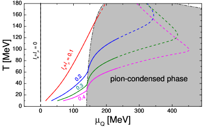
Figure 1: The phase diagram of an interacting hadron resonance gas with pion condensation in the $\mu_{Q}$-$T$ plane. The dash-dotted line separates the pion condensed phase (shaded area) from the normal phase. The colored lines depict cosmic trajectories for different values of the lepton flavor asymmetries: the standard cosmic trajectory (black) and $l_{e}+l_{\mu}$ equal to 0.1 (red), 0.2 (blue), 0.3 (green), and 0.4 (magenta). In all cases $l_{e}=l_{\mu}$ and $l=l_{e}+l_{\mu}+l_{\tau}=0$. The dashed parts of the trajectories correspond to regions where the effective mass model cannot be reliably validated with the lattice data.

The QCD pressure thus consists of the pressure of three pion species, each described by an effective mass model, and by contributions of the rest of the hadrons and resonances that are modeled as free particles:

$$p_{\rm QCD}(T,\mu_{B},\mu_{Q})=\sum_{i\in\pi}p_{i}^{\rm EM}(T,\mu_{i})+\sum_{j}\,p_{j}^{\rm id}(T,\mu_{j}).$$ (5)

Here $\mu_{j}=B_{j}\mu_{B}+Q_{j}\mu_{Q}$ with $B_{j}$ and $Q_{j}$ being the baryon and electric charge of hadron species $j$, respectively. The index $i$ sums over the three pion species and the index $j$ sums over all hadrons excluding pions. We include all established light flavored and strange hadrons listed in Particle Data Tables Olive et al. (2014).

All the conserved charge densities and the entropy density entering Eqs. (1)-(3) are calculated as the corresponding derivatives of the pressure function (4): $n_{i}=\partial p/\partial\mu_{i}$ for $i=B,Q,e,\mu,\tau$, and $s=\partial p/\partial T$. For given values of the baryon and lepton asymmetries $b$ and $l_{\alpha}$, we evaluate the cosmic trajectory in the temperature range $10<T<180$ MeV by numerically solving Eqs. (1)-(3) for the chemical potentials at each temperature. The numerical solution is achieved using Broyden’s method Broyden (1965). The procedure is implemented within an extended version of the open source Thermal-FIST package Vovchenko and Stoecker (2019). We tested this procedure by reproducing the cosmic trajectories reported in Ref. Wygas et al. (2018) using the HRG model.

Cosmic trajectories.

We fix $b=8.6\cdot 10^{-11}$ and perform a parametric scan in $l_{e}$ and $l_{\mu}$. As the restriction $|l|<0.012$ on the total lepton asymmetry is rather strong we shall set $l_{\tau}=-(l_{e}+l_{\mu})$, meaning that we have a vanishing total lepton asymmetry ($l=0$) in all our calculations. For each value of $l_{e}$ and $l_{\mu}$, we start calculations at $T=10$ MeV, where all cosmic trajectories are very similar, and gradually increase the temperature. If the cosmic trajectory enters the phase with a Bose-Einstein condensate of pions, we register the temperature $T_{\rm cond}$ where the trajectory crosses the pion condensation boundary.

Our calculations reveal that $T_{\rm cond}$ depends mainly on the sum $l_{e}+l_{\mu}$ of the electron and muon lepton asymmetries, whereas the dependence on the difference $l_{e}-l_{\mu}$ is mild. This is shown in Fig. 2, where we depict the dependence of the temperature $T_{\rm cond}$ on the sum $l_{e}+l_{\mu}$. The difference $l_{e}-l_{\mu}$ is varied in a range $|l_{e}-l_{\mu}|<0.5$, giving the narrow black uncertainty band in Fig. 2. At temperatures between $T_{\rm cond}$ and the chiral crossover pseudocritical temperature $T_{\rm pc}\approx 160$ MeV the cosmic matter is in a pion-condensed phase. We find that pion condensation occurs in the early Universe at $T<160$ MeV if the following condition is met:

$$|l_{e}+l_{\mu}|\gtrsim 0.1\leavevmode\nobreak\ .$$ (6)

Pion condensation is not observed at smaller absolute values of $l_{e}+l_{\mu}$. The relation (6) can therefore be regarded as a universal criterion for pion condensation in the early Universe. Positive values of $l_{e}+l_{\mu}$ correspond to $\pi^{+}$ condensation, while negative $l_{e}+l_{\mu}$ imply $\pi^{-}$ condensation.

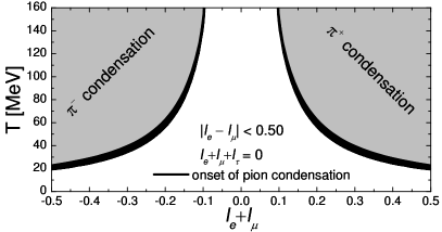
Figure 2: Dependence of the pion condensation onset temperature on the sum $l_{e}+l_{\mu}$ of electron and muon flavor asymmetries. The bands result from a variation of the difference of electron and muon asymmetries in a range $|l_{e}-l_{\mu}|<0.50$.

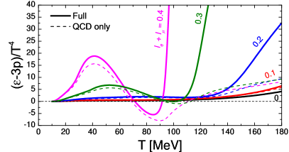
Figure 3: Temperature dependence of the interaction measure, $(\varepsilon-3p)/T^{4}$ along the cosmic trajectory for different values of the lepton flavor asymmetries: $l_{e}+l_{\mu}=0$ (black), 0.1 (red), 0.2 (blue), 0.3 (green), and 0.4 (magenta). In all cases $l_{e}+l_{\mu}+l_{\tau}=0$.

The temperature dependence of $\mu_{Q}$ is shown in Fig. 1 for several different values of lepton flavor asymmetries in the range $0\leq l_{e}+l_{\mu}\leq 0.4$. These values are motivated by various theoretical predictions to explain the baryon and lepton asymmetry in the early universe, see Refs. Affleck and Dine (1985); Stuke et al. (2012); Casas et al. (1999); McDonald (2000); Abazajian et al. (2005); Ichikawa et al. (2004). For $l_{e}+l_{\mu}=0$ one essentially recovers the standard cosmological trajectory where $\mu_{Q}$ is very close to zero throughout and far away from the pion condensed phase. For sufficiently large absolute values of $l_{e}+l_{\mu}$ [see Eq. (6)], the cosmic trajectory crosses the pion condensation boundary. The kink-like structure in the cosmic trajectory, predominantly visible for the $l_{e}+l_{\mu}=0.4$ case at $T\approx 95$ MeV, is associated with a rapid growth of the lepton chemical potentials.

The equation of state exhibits an interesting behavior for trajectories that enter the pion condensed phase. Of particular interest is the interaction measure, $(\varepsilon-3p)/T^{4}$. The interaction measure is negative deep in the pion-condensed phase at moderate temperatures (see Fig. 3) – a distinctive feature of the pion condensed phase also seen in lattice QCD calculations. Figure 3 depicts the temperature dependence of $(\varepsilon-3p)/T^{4}$ along the cosmic trajectory for the four different cases of positive $l_{e}+l_{\mu}$ values discussed above. The behavior of these two quantities is significantly affected at large lepton asymmetries. For $|l_{e}+l_{\mu}|\gtrsim 0.3$ the cosmic trajectory passes through a region with negative $(\varepsilon-3p)/T^{4}$, as illustrated by the magenta curve in Fig. 3 for $l_{e}+l_{\mu}=0.4$. Negative interaction measure correlates with large sound velocities that go above the conformal limit of $c_{s}^{2}=1/3$. The interaction measure grows to large values $(\varepsilon-3p)/T^{4}\gtrsim 10$ at larger temperatures. This drastic rise is a consequence of large lepton chemical potentials at these temperatures, which emerge from lepton flavor number conservation.

Effects on the spectrum of PGWs.

Due to the presence of a nonvanishing lepton asymmetry and the possible formation of the pion-condensed phase, the equation of state before big bang nucleosynthesis (BBN) can change, which will leave an imprint on the PGW spectrum Hajkarim et al. (2019); Hajkarim and Schaffner-Bielich (2020); Saikawa and Shirai (2018); Schettler et al. (2011).

The evolution of each polarization $\lambda$ of tensor perturbation $h$ for a mode $k$ in cosmology is given by Mukhanov et al. (1992); Mukhanov (2005)

$$h_{{\bf k},\lambda}^{\prime\prime}+2\frac{a^{\prime}}{a}h_{{\bf k},\lambda}^{\prime}+k^{2}h_{{\bf k},\lambda}=0\,,$$ (7)

where the ${}^{\prime}\equiv d/d\eta$ is the derivative with respect to conformal time $\eta$ and $a$ is the scale factor ($ad\eta=dt$, $t$ is the cosmic time). The primordial tensor perturbation can be written in terms of the transfer function $X$, tensor perturbation amplitude $h_{\bf k,\lambda}^{prim}$ and tensor power spectrum parameterized with respect to a characteristic scale $\tilde{k}=0.05$ Mpc^-1

$$h_{\bf k,\lambda}(\eta)\equiv h_{\bf k,\lambda}^{prim}X(k,\eta),\,\,\mathcal{P}_{T}=\sum_{\lambda}|h^{prim}_{\bf k,\lambda}|^{2}=A_{T}\left(\frac{k}{\tilde{k}}\right)^{n_{T}},$$ (8)

where $A_{T}=r\,A_{S}$ and $A_{S}$, $n_{T}$ are scalar and tensor perturbation amplitudes, and the tensor spectral index, respectively. The tensor to scalar ratio denoted by $r$ has an upper limit from measurements by PLANCK of $r\lesssim 0.07$ Akrami et al. (2020); Aghanim et al. (2020).

To compute the temporal evolution of the scale factor one needs to solve the Friedmann equation ($H^{2}=({\dot{a}}/a)^{2}=(8\pi/3M_{Pl}^{2})\varepsilon$, $M_{Pl}=1.22\times 10^{19}$ GeV). We solve Eq. (7) for a mode $k$ using (8) until horizon crossing fir , i.e. when $k=|{\bf k}|=a(\eta_{h})H(\eta_{h})$, then we use the WKB (Wentzel, Kramers, Brillouin) approximation for the PGW afterwards until today Watanabe and Komatsu (2006); Bernal and Hajkarim (2019). Using Eqs. (7) and (8) the relic density of PGWs for different frequencies $\nu=k/2\pi$ at today ($a_{0}$) can be computed from Watanabe and Komatsu (2006); Bernal and Hajkarim (2019)

$$\Omega_{\text{GW}}(k,\eta_{0})=\frac{\mathcal{P}_{T}(k)\left[X^{\prime}(k,\eta_{0})\right]^{2}}{24a_{0}^{2}H_{0}^{2}}\,.$$ (9)

Using the equations of state computed for different lepton asymmetry values, for which the cosmic trajectory can enter the pion condensed regime, one can estimate the PGW spectrum by using Eqs. (7)-(9). We consider entropy conservation ($s\,a^{3}=const.$) and use the number of degrees of freedom after neutrino decoupling Drees et al. (2015) to find the relation between the scale factor and the temperature. The PGW relic spectra are shown in Fig. 4. As the lepton asymmetry increases, so does the amplitude of the spectrum because the entropy, energy and pressure densities become larger. Moreover, the formation of pion condensation can enhance the PGW due to the change of equation of state. Pulsar timing arrays, such as the Square Kilometre Array (SKA) Janssen et al. (2015); Weltman et al. (2020), can measure the predicted PGW spectrum especially around the QCD phase transition if it is scale invariant ($n_{T}=0$) or blue-tilted ($n_{T}>0$). The LISA experiment Amaro-Seoane et al. (2017) can also measure such effects at higher frequencies. The lepton asymmetry at BBN time and afterwards is constrained by cosmic microwave background measurements. Since nonvanishing lepton asymmetry and pion condensation before BBN can modify the PGW spectrum, GW observatories with high sensitivity are able to measure these effects in the early Universe.

Impact on the formation of PBHs.

The population of primordial black holes that formed in the early Universe depends on the Hubble rate and the total mass within the Hubble horizon Byrnes et al. (2018); Widerin and Schmid (1998); Sobrinho et al. (2016); Jedamzik (1997); Schmid et al. (1999); Niemeyer and Jedamzik (1998, 1999). As mentioned earlier, a nonvanishing lepton asymmetry and a pion condensed phase modify the Hubble rate thereby modifying the production of PBHs in specific range of masses. The horizon mass, defined as $M_{h}=\frac{4\pi}{3}H^{-3}\varepsilon\,$  Carr (1975); Carr and Hawking (1974), relates a given temperature in the early Universe to the horizon mass and later on to a typical black hole mass $M_{\text{BH}}$. Figure 5 shows the fraction $f_{\text{PBH}}$ of PBHs with respect to total cold dark matter (CDM) abundance for different lepton asymmetry cases (see Ref. pbh for the technical details of the calculation). The presence of pion condensation is signalled by a modification of $f_{\text{PBH}}$ at masses larger than one solar mass.

The parameter $f_{\text{PBH}}$ can be indirectly measured by different experiments. The fraction of PBHs with masses $10^{-6}M_{\odot}\lesssim M_{\text{BH}}\lesssim 10^{3}M_{\odot}$ from some experimental constraints (OGLE, HSC, Caustic, EROS, MACHO) should be $f_{\text{PBH}}\lesssim 0.05$ sec ; Niikura et al. (2019a, b); Tisserand et al. (2007); Allsman et al. (2001); Oguri et al. (2018). The SKA Janssen et al. (2015); Weltman et al. (2020) and LISA Amaro-Seoane et al. (2017) can also indirectly constrain the fraction of PBHs by putting limits on the induced PGWs from curvature perturbation or using GWs produced by coalescing events Wang et al. (2019); Bartolo et al. (2019); Hajkarim et al. (2019).

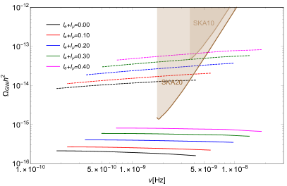
Figure 4: PGW relic density for different lepton asymmetry values and using the amplitude of scalar perturbation $A_{S}=2.1\times 10^{-9}$, the scale invariant $n_{T}=0$ (solid lines) and the scale dependent $n_{T}=0.25$ (dashed lines) tensor power spectrum from the upper bound on the tensor to scalar perturbation ratio $r=0.07$ of PLANCK. The future constraints that can be reached by the SKA over 10 and 20 years of operation are also shown Janssen et al. (2015); Weltman et al. (2020).

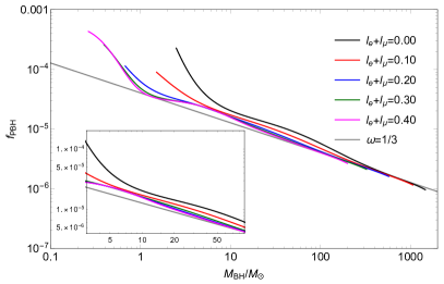
Figure 5: The fraction of PBHs with respect to PBH masses for different lepton asymmetry values (different colors) assuming the scale invariant Gaussian density perturbation and the value of the density spectral index $n_{M}=0$ pbh . The gray line denotes the result for a purely radiation dominated background fluid.

Summary.

The present analysis of cosmic trajectories at non-vanishing lepton flavor asymmetries reveals a simple criterion for the onset of pion condensation in the early Universe – it occurs when the total electron and muon asymmetry parameter is sufficiently large, $|l_{e}+l_{\mu}|\gtrsim 0.1$. This result does not exhibit large sensitivity to the modeling of pion interactions. Asymmetries beyond this value lead the system deep inside the pion condensed phase, affecting its equation of state considerably. The possible presence of such a Bose-Einstein condensed phase of pions would have significant cosmological implications such as the strong enhancement of the spectrum of PGWs and the change of the fraction of PBHs with mass larger than one solar mass. The experimental signatures of pion condensation from the early Universe can be probed by pulsar timing and GW detectors. The recent BHs merger event of LIGO GW190521 can be from PBHs produced during the pion condensation epoch Abbott et al. (2020a, b).

Pion condensation could also affect big bang nucleosynthesis. If the pion condensed phase is present, spheres of pions and leptons – the pion stars – can form which are stabilized by the high density of neutrinos due to the high lepton chemical potentials Carignano et al. (2017); Brandt et al. (2018b); Andersen and Kneschke (2018). Typical pion star masses will be in the range of a few solar masses when the early Universe leaves the pion condensed phase. The neutrinos will diffuse out of the pion stars on the timescale of weak interactions. The situation is similar to the one for proto-neutron stars where neutrinos leave on the timescale of several seconds. Hence, pion stars would decay around the time of BBN. The produced high energy leptons would influence the abundances of primordially produced nuclei, which could be addressed by a modified BBN simulation.

Supplemental material

I Effective mass model for pion condensation

We use a quasiparticle (effective mass) approach to describe interacting pions with a pion-condensed phase. Outside of the pion condensed phase, the pressure of a single pion species in the effective mass model reads Savchuk et al. (2020)

$$p_{\pi}^{\rm EM}(T,\mu_{\pi};m^{*})=p^{\rm id}_{\pi}(T,\mu_{\pi};m^{*})+p_{f}(m^{*}).$$ (10)

Here $\pi\in\pi^{+},\pi^{-},\pi^{0}$. The rearrangement term $p_{f}(m^{*})$ is a consequence of interactions. It ensures a proper counting of the interaction energy and preserves the thermodynamic consistency in the quasiparticle model. For instance, it ensures that the quasiparticle pion number density, $n_{\pi}^{\rm EM}=n^{\rm id}_{\pi}(T,\mu_{\pi};m^{*})$, satisfies a thermodynamic relation $n_{\pi}^{\rm EM}=(\partial p_{\pi}^{\rm EM}/\partial\mu_{\pi})_{T}$, correctly taking into account the medium dependence of the effective mass, $m^{*}(T,\mu)$. The specific form of $p_{f}(m^{*})$ defines the quasiparticle model. Here we take $p_{f}(m^{*})$ in the form

$$p_{f}(m^{*})=\frac{(m^{*})^{2}f_{\pi}^{2}}{4}\,\left[1-\frac{m_{\pi}^{2}}{(m^{*})^{2}}\right]^{2}\leavevmode\nobreak\ ,$$ (11)

chosen to match the model to chiral perturbation theory and lattice QCD results in the pion-condensed phase at $T=0$ (see below). The pressure at a given $T$ and $\mu_{\pi}$ has to be maximized with respect to $m^{*}$, resulting in a gap equation $(\partial p_{\pi}^{\rm EM}/\partial m^{*})_{T,\mu}=0$:

$$p_{f}^{\prime}(m^{*})=n^{\rm id}_{\sigma}(T,\mu_{\pi};m^{*})\leavevmode\nobreak\ .$$ (12)

Here $n^{\rm id}_{\sigma}(T,\mu_{\pi};m^{*})\equiv-\partial p_{\pi}^{\rm id}/\partial m^{*}$ is the scalar density of an ideal gas of pions with mass $m^{*}$. A numerical solution to the gap equation determines $m^{*}$ at given $T$ and $\mu_{\pi}$, allowing to calculate all other thermodynamic quantities through Eq. (11).

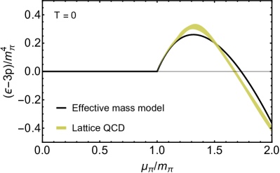
Figure 6: The dependence of the normalized trace anomaly $(\varepsilon-3p)/m_{\pi}^{4}$ on the normalized pion chemical potential $\mu_{\pi}/m_{\pi}$, evaluated in the effective mass model at $T=0$. The yellow band depicts lattice QCD results from Ref. Brandt et al. (2018b).

The transition to the pion-condensed phase takes place when the effective pion mass becomes equal to the chemical potential, $m^{*}=\mu_{\pi}$. The equation determining the transition line in the $\mu_{\pi}$-$T$ plane reads Savchuk et al. (2020)

$$p_{f}^{\prime}(\mu_{\pi})=n^{\rm id}_{\sigma}(T,\mu_{\pi};m^{*}=\mu_{\pi})\leavevmode\nobreak\ .$$ (13)

The effective mass equals the chemical potential in the phase diagram region with a pion condensate, $m^{*}=\mu_{\pi}$ for $\mu_{\pi}\geq\mu_{\rm cond}$, as a consequence of interactions between thermal and condensed pions Barz et al. (1989). Here $\mu_{\rm cond}$ is the pion chemical potential at pion condensation boundary. Therefore, the pressure in this phase reads reads

$$p_{\pi}^{\rm EM}(T,\mu_{\pi})=p^{\rm id}(T,\mu_{\pi};m^{*}=\mu_{\pi})+p_{f}(\mu_{\pi}).$$ (14)

At $T=0$, the pion number density $n_{\pi}^{\rm EM}=(\partial p_{\pi}^{\rm EM}/\partial\mu_{\pi})_{T}$ reads

$$n_{\pi}^{\rm EM}(T=0,\mu_{\pi}) =p_{f}^{\prime}(\mu)\,\theta(\mu-m_{\pi})$$

$$=\frac{\mu_{\pi}\,f_{\pi}^{2}}{2}\left[1-\frac{m_{\pi}^{4}}{\mu_{\pi}^{4}}\right]\,\theta(\mu-m_{\pi}).$$ (15)

Equation (I) matches the result of leading-order chiral perturbation theory Son and Stephanov (2001), which for $f_{\pi}=133$ MeV describes well the available lattice QCD data on isospin density at $T=0$ Brandt et al. (2018b). Recently, these chiral perturbation theory predictions have been backed up by next-to-leading-order calculations, both for the density and for the equation of state Adhikari and Andersen (2020a, b, c); Adhikari et al. (2020).

II Lattice simulations

Here we describe the details of our first-principles lattice QCD simulations at nonzero isospin density. On the one hand, the lattice results at (approximately) zero temperature are used to guide the construction of the effective mass model described above. Here we use our data at a single lattice spacing from Ref. Brandt et al. (2018b). On the other hand, the finite-temperature results serve to test the validity range of the model at nonzero isospin and zero baryon density. To this end we employ our data from Refs. Brandt et al. (2018a); Brandt and Endrődi (2019) on four lattice spacings.

To simulate the path integral $\mathcal{Z}$ we take the tree-level Symanzik-improved gauge action and $2+1$ flavors of rooted staggered quarks with physical masses Borsányi et al. (2010). The isospin chemical potential $\mu_{I}$ enters the Dirac operator via the quark chemical potentials $\mu_{u}=-\mu_{d}=\mu_{I}/2$, while $\mu_{s}=0$. Comparing to the standard basis with baryon and charge chemical potentials, one can read off $\mu_{Q}=\mu_{I}$, $\mu_{B}=-\mu_{I}/2$. The simulations therefore correspond to a situation with a specific linear combination of baryon and charge chemical potentials, which only couples to hadron species containing an unequal number of up and down quarks (predominantly charged pions). To be able to perform the simulations, we further need to introduce an auxiliary pionic source $\lambda>0$ that is extrapolated to zero at the end of the analysis. The role of the $\lambda$ parameter is twofold. First, it triggers the spontaneous symmetry breaking corresponding to pion condensation in a finite volume. Second, it serves to stabilize the theory in the infrared by making the Goldstone boson of the pion condensed phase slightly massive Brandt et al. (2018a).

To calculate the equation of state, our primary observable is the isospin density

$$n_{I}(T,\mu_{I})=\frac{T}{V}\frac{\partial\log\mathcal{Z}}{\partial\mu_{I}}\,.$$ (16)

The details of the $\lambda\to 0$ extrapolation of this observable are explained in Ref. Brandt and Endrődi (2019) and in the following we work with the so extrapolated quantity. From $n_{I}$, we can calculate $\Delta\mathcal{O}(T,\mu_{I})\equiv\mathcal{O}(T,\mu_{I})-\mathcal{O}(T,0)$ for any observable $\mathcal{O}$. In particular, the pressure difference and the trace anomaly difference can be constructed as

$$\Delta p(T,\mu_{I}) =\int_{0}^{\mu_{I}}\!\!\!\!\textmd{d}\mu_{I}^{\prime}\,n_{I}(T,\mu_{I}^{\prime})\,,$$ (17)

$$\Delta I(T,\mu_{I}) =\mu_{I}n_{I}(T,\mu_{I})\!+\!\int_{0}^{\mu_{I}}\!\!\!\!\textmd{d}\mu_{I}^{\prime}\left(T\frac{\partial}{\partial T}-4\right)n_{I}(T,\mu_{I}^{\prime})\,.$$ (18)

The zero-temperature results for $n_{I}$ near $\mu_{I}=m_{\pi}$ are well-described by the chiral perturbation theory formula (I) with $f_{\pi}=133(4)\textmd{ MeV}$ Brandt et al. (2018b); Adhikari and Andersen (2020a, b, c); Adhikari et al. (2020). This is smoothly matched by a spline interpolation for $n_{I}(\mu_{I})$ at higher values of the chemical potential. The interaction measure is determined via Eq. (18) – note that at zero temperature $\Delta I=I$ and, moreover, the first contribution to the integral in $\Delta I$ of Eq. (18) vanishes, simplifying this expression considerably. The so obtained curve is plotted in Fig. 6 as the yellow band.

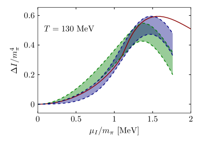
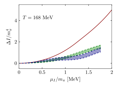
Figure 7: The trace anomaly difference as a function of $\mu_{I}$ at two different temperatures on our $N_{t}=10$ (green) and $N_{t}=12$ (blue) lattice ensembles, compared to the effective mass model (red curve).

For testing the effective mass model at $T>0$ we concentrate on $\Delta I$ because compared to other observables it is found to contain the least amount of lattice discretization errors. The integrals and the derivatives in Eq. (18) need to be evaluated numerically. To this end we fit $n_{I}(T,\mu_{I})$ via a two-dimensional spline surface. The spline nodepoints are drawn from a Monte-Carlo procedure with the goodness of the fit playing the role of the action, providing a direct estimate of systematic errors (see Ref. Brandt and Endrődi (2016) for more details). The $\mu_{I}$-dependence of $\Delta I$ is plotted for two representative values of the temperature in Fig. 7. Here we include the results for our two finest lattice spacings, $N_{t}=10$ and $N_{t}=12$. (The continuum limit at constant $T$ corresponds to $N_{t}\to\infty$, but we do not carry out this extrapolation here.) The model is found to capture the notable features of the lattice data qualitatively. A quantitative description is obtained if neither $T$ nor $\mu_{I}$ are too large. In particular, sizeable deviations are visible above the chiral restoration temperature, because the effective mass model does not contain the details of the physics of this phase transition.

To make the comparison between the $N_{t}=12$ lattice results and the model more systematic, in Fig. 8 we show the deviation between the two in the form of a heat plot. Here we normalize by the error $\sigma$ of the lattice results – therefore a value of $n$ indicates a difference by $n$ standard deviations. The plot shows substantial differences for $\mu_{I}>m_{\pi}$ at high temperatures as well as slight deviations near the boundary of the pion condensed phase. We take the contour line at $3$ standard deviations as a marker and consider the model reliable in the parameter range where

$$\frac{|\Delta I-\Delta I^{\rm EM}|}{\sigma(\Delta I)}\leq 3\,,$$ (19)

with $\Delta I^{\rm EM}$ being the subtracted interaction measure in the effective mass model. This range is indicated by the solid line sections of the cosmic trajectories in Fig. 1 of the main text.

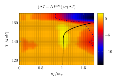
Figure 8: Heat plot of the deviation between the effective mass model and the lattice results for the trace anomaly difference $\Delta I$. For the latter our finest, $N_{t}=12$ ensembles are used. The deviation is normalized by the error of the lattice data. The solid black line indicates the lattice result for the pion condensation boundary, while the dashed line denotes the contour of $3$.

The above comparisons were performed at nonzero isospin chemical potential $\mu_{I}$, where lattice results are available. For the analysis of the cosmic trajectory, the model is employed instead at nonzero charge chemical potential $\mu_{Q}$ (as well as low baryon chemical potential $\mu_{B}$). At zero temperature, $\mu_{I}$ and $\mu_{Q}$ can be identified as long as the only charged states that contribute to the equation of state have zero strangeness and zero baryon number. This is the case for $\mu_{I}<m_{K}$ (even in this case, kaon condensation is not expected to occur if a pion condensate is already present Mannarelli (2019)) and sufficiently low $\mu_{B}$ as is the case for the parameters considered in this paper.

Contrary to the identification $\mu_{I}=\mu_{Q}$ at zero temperature, for $T>0$ the different couplings of the two chemical potentials to hadronic states becomes relevant and the equation of state differs in the two cases. Nevertheless, in the effective mass model the pion condensation boundary expressed in $\mu_{I}$ or in $\mu_{Q}$ remains the same, because interactions between pions and other hadrons are neglected in the model. The difference between the critical lines, $\mu_{Q}^{\rm crit}(T)$ and $\mu_{I}^{\rm crit}(T)$ can be estimated using lattice results for the estimators of the convergence radii of the corresponding Taylor series around $\mu_{Q}=\mu_{I}=0$. In particular, we consider the expansions of the pressure,

$$\frac{p}{T^{4}}=\frac{c_{2}^{I,Q}}{2}\left(\frac{\mu_{I,Q}}{T}\right)^{2}+\frac{c_{4}^{I,Q}}{24}\left(\frac{\mu_{I,Q}}{T}\right)^{4}+\ldots$$ (20)

and the estimators for the convergence radius for the susceptibilities $\chi_{I,Q}=\partial^{2}p/\partial\mu_{I,Q}^{2}$. We use the Taylor coefficients determined in Ref. Borsányi et al. (2012) for our action and lattice spacings. The leading estimator

$$\frac{r_{2}(\chi_{I,Q})}{T}=\sqrt{\frac{2c_{2}^{I,Q}}{c_{4}^{I,Q}}}\,,$$ (21)

for the isospin direction was found to give a remarkably good approximation to the true critical line, $\mu_{I}^{\rm crit}$ Brandt and Endrődi (2019). We assume this is also the case for the expansion in $\mu_{Q}$. Thus we approximate the critical line in the electric charge direction by

$$\mu_{Q}^{\rm crit}\approx\mu_{I}^{\rm crit}\cdot\frac{r_{2}(\chi_{Q})}{r_{2}(\chi_{I})}\,.$$ (22)

For the second factor we use the lattice results Borsányi et al. (2012) above and ideal HRG with quantum statistics below a matching temperature of $105\textmd{ MeV}$. The $N_{t}=12$ results for this approximation, together with the corresponding directly determined isospin critical line $\mu_{I}^{\rm crit}$ Brandt et al. (2018a); Brandt and Endrődi (2019), are plotted in Fig. 9.

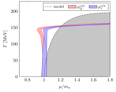
Figure 9: The critical lines $\mu_{Q}^{\rm crit}$ and $\mu_{I}^{\rm crit}$ as obtained on $N_{t}=12$ lattices from the approximation in Eq. (22) and from direct simulations, respectively. The critical line from the effective mass model is included for comparison.

Comparing to the effective mass model, quantitative differences are observed for $T\gtrsim 80\textmd{ MeV}$. While this bound is comparable to recent results in chiral perturbation theory to next-to-leading order Adhikari et al. (2020), where the agreement persists up to about $T\gtrsim 40\textmd{ MeV}$, other models, such as the Nambu-Jona-Lasinio He et al. (2005) or the Polyakov loop-extended quark meson model Adhikari et al. (2018); Folkestad and Andersen (2019), for instance, show better agreement, both qualitatively and quantitatively, with the lattice phase diagram (see also Fig. 9 of Ref. Mannarelli (2019)). In particular, both models reproduce the steep rise in combination with the leveling-off of the BEC phase boundary at large $\mu_{I}$. Nonetheless, the qualitative agreement between the effective mass model and the lattice data together with the fact that the lattice results for $\mu_{I}^{\rm crit}$ and $\mu_{Q}^{\rm crit}$ do not differ by more than a few percents again confirms that our model represents a reasonable approximation to the phase diagram at nonzero isospin (charge) densities. In addition, the inclusion of further hadrons and resonances in the effective mass model is straightforward.

III Primordial Black Holes Formation

At the time of PBH formation a region of the Universe within the Hubble horizon starts to collapse due to local inhomogeneities amounting to

$$\beta(M)=\frac{M_{eq}}{M}\beta_{eq}\,.$$ (23)

The relation between the amplitude of the density perturbation $\delta$, the PBH mass $M_{\text{BH}}$ and the horizon mass $M_{h}$ can be defined as Niemeyer and Jedamzik (1998, 1999)

$$\delta=\left(\frac{M_{\text{BH}}}{KM_{h}}\right)^{\frac{1}{\gamma}}+\delta_{c}\,.$$ (24)

The parameters in Eq. (24) are obtained from numerical simulations to be $K=3.3$ and $\gamma=0.36$ Evans and Coleman (1994); Koike et al. (1995); Niemeyer and Jedamzik (1998, 1999); Musco et al. (2009, 2005). The parameter $\delta_{c}$ is the threshold for PBH formation where different estimates for it exist in the literature Jedamzik (1997); Niemeyer and Jedamzik (1998, 1999); Musco et al. (2005, 2009); Harada et al. (2013); Escrivà et al. (2020). Here we assume that this threshold in a cosmological background slightly deviates from the one of a purely radiation dominated Universe ($\omega=p/\varepsilon=1/3$) which is estimated to be $\delta_{c}\simeq 0.41$ Harada et al. (2013); Escrivà et al. (2020). Variation of $\delta_{c}$ due to different lepton asymmetry values is shown in Fig. 10.

The fraction of PBHs $\Omega_{\text{PBH}}$ with respect to the total cold dark matter (CDM) abundance $\Omega_{\text{CDM}}$ reads Byrnes et al. (2018)

$$f_{\text{PBH}}(M_{\text{\text{BH}}})= \frac{1}{\Omega_{\text{CDM}}}\int_{0}^{\infty}\frac{2dM_{h}}{\sqrt{2\pi\sigma(M_{h})^{2}}}\frac{M_{\text{BH}}}{\gamma M_{h}}\times$$

$$\exp\left[-\frac{\delta^{2}(M_{h})}{2\sigma^{2}(M_{h})}\right]\left(\frac{M_{\text{BH}}}{KM_{h}}\right)^{\frac{1}{\gamma}}\sqrt{\frac{M_{eq}}{M_{h}}}\,.$$

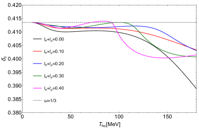
Figure 10: Threshold of primordial black hole formation versus horizon crossing temperature for different values of the lepton asymmetry.

The mass or scale dependence of the density perturbation width can be assumed to be Byrnes et al. (2018)

$$\sigma^{2}(M_{h})=0.003\left(\frac{M_{h}}{10M_{\odot}}\right)^{n_{M}}\,.$$ (26)

The density spectral index $n_{M}$ can be related to the scalar spectral index $n_{S}-1\simeq-2n_{M}$, where $n_{S}\simeq 0.96$ Akrami et al. (2020); Aghanim et al. (2020). We choose the benchmark value of $n_{M}=0$ to compute the fraction of PBH from Eq. (III). The parameter $f_{\text{PBH}}$ for masses smaller than $M_{\odot}$ increases (decreases) when $n_{M}$ is negative (positive). However, $f_{\text{PBH}}$ increases (decreases) for larger masses, respectively. For a fixed $n_{M}$ as lepton asymmetry increases the value of $f_{\text{PBH}}$ will change depending on the behavior of $\omega$ or $\delta_{c}$ and the energy and pressure density. When $\delta_{c}$ increases (decreases) the fraction of PBH decreases (increases).