Adaptive preferential sampling in phylodynamics

Abstract

Longitudinal molecular data of rapidly evolving viruses and pathogens provide information about disease spread and complement traditional surveillance approaches based on case count data. The coalescent is used to model the genealogy that represents the sample ancestral relationships. The basic assumption is that coalescent events occur at a rate inversely proportional to the effective population size $N_{e}(t)$, a time-varying measure of genetic diversity. When the sampling process (collection of samples over time) depends on $N_{e}(t)$, the coalescent and the sampling processes can be jointly modeled to improve estimation of $N_{e}(t)$. Failing to do so can lead to bias due to model misspecification. However, the way that the sampling process depends on the effective population size may vary over time. We introduce an approach where the sampling process is modeled as an inhomogeneous Poisson process with rate equal to the product of $N_{e}(t)$ and a time-varying coefficient, making minimal assumptions on their functional shapes via Markov random field priors. We provide scalable algorithms for inference, show the model performance vis-a-vis alternative methods in a simulation study, and apply our model to SARS-CoV-2 sequences from Los Angeles and Santa Clara counties. The methodology is implemented and available in the R package adapref.

Keywords: coalescent process, population size, Poisson processes, Markov random fields.

1 Introduction

Molecular sequence data, within the framework of phylodynamics (Grenfell et al., 2004), is increasingly being used to track disease spread caused by rapidly evolving viruses and pathogens such as Influenza viruses (Rambaut et al., 2008), Zika (Faria et al., 2016), and SARS-CoV-2 (Hadfield et al., 2018). The coalescent process (Kingman, 1982b, a), a probability model of gene genealogies, depends on a parameter called effective population size $N_{e}(t)$, which is a time-varying measure of genetic diversity. When disease dynamics can be modeled by simple epidemiological models such as Susceptible-Infected-Recovered, the coalescent effective population size can be expressed in terms of transmission rates and prevalence (Volz et al., 2009; Frost and Volz, 2010). Accurate and scalable inference for $N_{e}(t)$ is thus relevant to estimate epidemiological parameters of great interest in public health. Although this work is motivated by applications in molecular epidemiology of infectious diseases, estimation of $N_{e}(t)$ is an active area of research with applications ranging across many other scientific domains such as conservation biology and population genetics (e.g. Shapiro et al. (2004); Huff et al. (2010); Lorenzen et al. (2011)).

A common feature in these applications is that genetic data are collected sequentially (heterochronous samples). In viral studies, samples are collected and sequenced when infected individuals attend clinics, hospitals, or testing centers. In ancient DNA studies, specimens are dated according to the time they lived, estimated through radiocarbon dating or other techniques. The coalescent typically models the gene genealogy conditionally on sampling dates, that is, the sampling dates are treated as censoring information (Felsenstein and Rodrigo, 1999). However, in some situations, it is reasonable to assume that samples are collected at a higher frequency when the population is large and at a lower frequency when the population is small: for example, at the onset of an epidemic, as the viral population grows and more people get infected, more resources may be allocated to monitor the viral spread, possibly leading to more molecular sequence collection. The number of SARS-CoV-2 sequences uploaded daily in GISAID offers some evidence of this claim (Shu and McCauley, 2017) (see the histogram in the supplementary material).

Karcher et al. (2016) study the scenario in which the sampling process depends on the population size, and show that an estimator of $N_{e}(t)$ that does not account for this dependence is biased. This issue was first discussed in the spatial statistics literature by Diggle et al. (2010), who term preferential sampling a situation in which the process that determines the data locations and the process under study are dependent. In this paper, we will introduce a new model that account for preferential sampling in a coalescent framework, while making minimal assumptions on $N_{e}(t)$, the sampling process, and their dependence.

Three estimators that incorporate preferential sampling into the coalescent framework have been proposed. Volz and Frost (2014) propose an estimator in the case that $N_{e}(t)$ grows exponentially and samples are collected as an inhomogeneous Poisson process with rate linearly dependent on the effective population size. Karcher et al. (2016) assume that $N_{e}(t)$ is a continuous function, and the samples are collected as an inhomogeneous Poisson process with rate $\lambda(t)=\exp(\beta_{0})N_{e}(t)^{\beta_{1}}$, for $\beta_{0},\beta_{1}\geq 0$, i.e. the dependence between the sampling process and the effective sample size is described by a parametric model. Recent work by Parag et al. (2020) weakens this assumption substantially, allowing for the dependence between the sampling process and effective population size to vary over time. The key assumption in Parag et al. (2020) is that the sampling rate depends linearly on $N_{e}(t)$ within a given time interval, but the linear coefficient changes across time intervals. The estimator of Parag et al. (2020), termed Epoch skyline plot (ESP), is an extension of the classic skyline plot estimator for $N_{e}(t)$ (Pybus et al., 2000), in which the sampling rate and the effective population size are both piecewise-constant, and the location and number of change points (boundary points of the time intervals) are either specified or inferred. As it is typical with skyline plots, the estimates are highly variable, rough, and highly dependent on the specification of change points locations and the number of piecewise-constant pieces used. All three works show that under correct model specification, accounting for preferential sampling leads to a more accurate estimation of $N_{e}(t)$ (in terms of absolute deviations to the true trajectory), and narrower credible regions.

Other non-coalescent approaches for phylodynamics, such as birth-death processes (Stadler, 2010), explicitly incorporate the sampling process by modeling the sampling dates as a partially observed death process where only a fraction of the population is observed. Stadler et al. (2013) extended previous work to allow sampling rates to vary through time. Volz and Frost (2014) show that in both, coalescent and birth-death processes alike, statistical power largely depends on the correct specification of the sampling process rate, rather than on the genealogical model. Hence, the need for a flexible modeling approach of the sampling process, adaptive to any possible scenarios encountered in applications.

There are a plethora of nonparametric estimators of $N_{e}(t)$ following the skyline plot (Pybus et al., 2000): among others, the generalized skyline plot (Strimmer and Pybus, 2001) and the Bayesian skyline plot (Drummond et al., 2005) reduce the high variance and roughness that characterize the skyline plot estimators. These methodologies require either fixing or estimating change-points in $N_{e}(t)$. A set of models that do not employ change-points but arbitrary discrete grids is based on Markov random fields (MRF): the Gaussian MRF (GMRF) (Minin et al., 2008; Palacios and Minin, 2012) allows for the recovery of smooth continuous trajectories; the Horseshoe MRF (HSMRF) (Faulkner et al., 2020) is an alternative to GMRF which is locally adaptive, i.e. it can successfully recover sharp changes in a trajectory and it is adaptive to a varying level of smoothness.

In this paper, we borrow from this literature and introduce an adaptive preferential sampling framework for phylodynamics, where the adaptivity follows from the fact that the dependence of the sampling process on $N_{e}(t)$ changes over time. The effective population size $N_{e}(t)$ is modeled as a latent parameter included in both, the coalescent and the sampling processes. The latter assumed to be an inhomogeneous Poisson process with rate $\lambda(t)=\beta(t)N_{e}(t)$, where $\beta(t)$ is a continuous function controlling the dependence on $N_{e}(t)$, analogous to that introduced by Parag et al. (2020). We a priori model $N_{e}(t)$ and $\beta(t)$ as two Markov random fields (MRF), with the flexibility of using either a GMRF or a HSMRF. The prior choice follows from the properties of the fields. The advantage of the proposed adaptive preferential sampling over the ESP estimator is that there is no need to specify (or estimate) the number and location of the change points of $\beta$ and $N_{e}$. Also, the resulting estimates are smooth and the high variability that characterizes skyline estimates disappears.

We develop the methodology assuming that a genealogy is available to the researcher and develop algorithms for inference under this framework. We test our model on simulated data and compare it to alternative methods, including both, estimators that account for preferential sampling and others that do not. We implement our method in the R package adapref, available at https://github.com/lorenzocapp/adapref, provide two algorithms for posterior approximation: a Hamiltonian MCMC and a Laplace approximation. We apply our method to SARS-CoV-2 sequences from California and study whether there is evidence of preferential sampling.

The rest of the paper proceeds as follows. In Section 2, we provide background on the coalescent process, the MRF priors on $N_{e}(t)$, and previous work on preferential sampling. In Section 3 we introduce the adaptive preferential sampling framework and explain how to approximate the posterior distribution of model parameters. Section 4 includes a simulation study, in which we test the new set of priors through simulated data and compare them to alternatives. In Section 5, we apply our method to two data sets of SARS-CoV-2 sequences from Santa Clara and Los Angeles counties in California. Section 6 concludes.

2 Background

2.1 Coalescent model

Coalescent models are continuous-time Markov chains used to model the set of ancestral relationships of a sample of $n$ individuals from a large population called gene genealogy. In the context of molecular epidemiology, a genealogy is a subset of the transmission history among the samples (Figure 1). Starting from the original work of Kingman (1982a), several extensions to the standard coalescent have been developed to incorporate more realistic population and sampling features, such as variable population size (Slatkin and Hudson, 1991), longitudinal sampling (also called heterochronous sampling) (Felsenstein and Rodrigo, 1999) and population structure (Hudson, 1990); Wakeley (2009) provides a good introduction to the subject. Coalescent processes can be characterized by two underlying processes: a jump chain defining the ancestral relationships represented by a binary tree topology and a pure death process that defines the timing of the coalescent events, i.e. the times when pairs of lineages meet their common ancestors. This sequence of holding times defines the branch length of the corresponding tree topology.

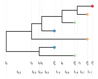
Figure 1: Example of a heterochronous genealogy. A genealogy of $7$ individuals sampled at 4 different times (color of tips) with multiplicities $(n_{1}=1,n_{2}=2,n_{3}=2,n_{4}=2)$. Sampling times are denoted by $(t^{s}_{k})_{1:4}$, coalescent times are denoted by $(t_{k})_{2:7}$ and $I_{i,j}$ denoted the interval lengths delimited by coalescent times and/or sampling times, i.e. every time there is a change in the number of lineages.

Let the vector $\textbf{n}{}=(n_{1},\ldots,n_{m})$ denote the sample sizes at times $\textbf{t}^{s}{}=(t^{s}_{1},\ldots,t^{s}_{m})$, with $m$ number of sampling points and $n$ total sample size. The process goes backward in time (from present toward the past): with $t^{s}_{1}=0$ denoting the present time, and $t^{s}_{j}>t^{s}_{j-1}$ for $j=2,\ldots,m$. Let $\textbf{t}{}=(t_{n+1},\ldots,t_{2})$ be the vector of coalescent times with $t_{n+1}=0<t_{n}<...<t_{2}$. Note that the subscript in $t_{k}$ is not the current number of extant lineages (often a convention in the coalescent literature) but the number of lineages that have yet to coalesce. Starting from $t=0$, vectors t and $\textbf{t}^{s}{}$ partition time into intervals (Figure 1). An interval ending with a coalescent event, say $t_{k}$, is denoted by $I_{0,k}$; the intervals that end with a sampling time within the interval $(t_{k+1},t_{k})$ are denoted as $I_{i,k}$, where $i\geq 1$ indexes all the sampling events in $(t_{k+1},t_{k})$. Formally, for every $k\in\{2,\ldots,n\}$, we define

$$I_{0,k}=[\max\{t_{k+1},t^{s}_{j}\},t_{k}),\quad\text{ where the maximum is taken over all }t^{s}_{j}<t_{k},$$

and for every $i\geq 1$ we set

$$I_{i,k}=[\max\{t_{k+1},t^{s}_{j-i}\},t^{s}_{j-i+1})\text{ with the max taken over all }t^{s}_{j-i+1}>t_{k+1}\text{ and }t^{s}_{j}<t_{k}.$$

With $n_{i,k}$ denoting the number of extant lineages during the time interval $I_{i,k}$. Figure 1 plots an example of a heterochronous genealogy with $\textbf{n}=(1,2,2,2)$, at times $\textbf{t}^{t}=(t^{s}_{1},\ldots,,t^{s}_{4})$ with $t^{s}_{1}=0$. In the interval $(t_{6},t_{5})$ there are two intervals: $I_{1,5}=[t_{6},t^{s}_{4})$, $I_{0,7}=[t^{s}_{4},t_{5})$.

The vector of coalescent times t is a random vector whose density with respect to the Lebesgue measure on $\mathbb{R}_{+}^{n-1}$ depends on two quantities: the coalescent factor $C_{i,k}:=\binom{n_{i,k}}{2}$, and the effective population size $N_{e}(t)$. The coalescent density can be factorized as the product of the conditional densities of $t_{k-1}$ given $t_{k}$, i.e.

$$p(\textbf{t}\mid\mathbf{s},\mathbf{n},N_{e}(t))=\prod_{k=n+1}^{3}p(t_{k-1}\mid t_{k},\mathbf{s},\mathbf{n},N_{e}(t))=\prod_{k=n+1}^{3}\frac{C_{0,k-1}}{N_{e}(t_{k-1})}\exp\left\{-\int_{I_{0,k-1}}\frac{C_{0,k-1}}{N_{e}(t)}{\rm d}t+\sum^{m}_{i=1}\int_{I_{i,k-1}}\frac{C_{i,k-1}}{N_{e}(t)}{\rm d}t\right\}.$$ (1)

A few remarks. First, the integral over $I_{i,k-1}$ accounts for the probability of no coalescence during $I_{i,k-1}$. It is zero if there are less than $i$ sampling times between $t_{k}$ and $t_{k-1}$. Second, conditionally on s, n and $t_{k}$, the coalescent factors can be computed exactly and $N_{e}(t)$ is the only unknown parameter, sampling times are assumed fixed.

Coalescent times can be alternatively viewed as the realization of an inhomogeneous point process with rate $C(t)N_{e}(t)^{-1}$, with the coalescent factor $C(t)$ being defined for all $t\geq 0$ by the notation above. This alternative view allows us to frame the problem of inferring $N_{e}(t)$ as that of inferring the intensity function of an inhomogeneous point process. Palacios and Minin (2013) is an example of how this representation is useful in inference and simulations.

2.2 Some priors for the effective population size

Markov random field-based priors on the log effective population trajectory allows smoothing without careful modeling of change points. They are computationally tractable thanks to the sparsity assumption in the covariance matrix of the field (Rue and Held, 2005). All MRF-based priors for phylodynamic inference share the assumption that the trajectory $N_{e}(t)$ is an unknown continuous function. The integral in (1) is numerically approximated by the Riemann sum at a regular grid of $M+1$ points $(k_{i})_{1:M+1}$, and one assumes that the trajectory $N_{e}(t)$ is well approximated by $\sum^{M+1}_{i=1}\exp\theta_{i}1(t\in(k_{i},k_{i+1}))$, with $\boldsymbol{\theta}=(\theta_{i})_{1:M}$. We stress that neither the grid cell boundaries $(k_{i})_{1:M+1}$ nor $M$ depend on t and $N_{e}(t)$, with the choice of $M$ commonly based on $n$ (Faulkner et al., 2020). A description of the discretized coalescent log-likelihood $\mathcal{L}(\boldsymbol{\theta}|\textbf{t})$ is given in detail in Palacios and Minin (2012) and Faulkner et al. (2020).

The Horseshoe Markov random field prior (HSMRF) for $\boldsymbol{\theta}$ (Faulkner et al., 2020) assumes that the $p$th order forward differences of $\boldsymbol{\theta}$ are independent and Horseshoe distributed (Carvalho et al., 2010), i.e.

$$\Delta^{p}\theta_{i}|\tau_{i}\sim N(0,\tau^{2}_{i})\,\ \,\ \,\ \,\ \tau_{i}|\gamma\sim C^{+}(0,\gamma)\,\ \,\ \,\ \,\ \gamma|\zeta\sim C^{+}(0,\zeta)\,\ \,\ \,\ \,\ \text{for}\,\,p+1\leq i\leq M-1,$$ (2)

where $C^{+}(0,a)$ is the standard half-Cauchy distribution with positive support with scale parameter $a$, $\tau_{i}$ are the local shrinkage parameters and $\gamma$ is the global smoothing parameter. To completely specify the prior, one sets $\theta_{1}\sim N(\mu,\sigma_{1}^{2})$, and for $p\geq 2$, the first p values of the field have running order q difference priors as follows:

$$\Delta^{q}\theta_{q}|a_{q}\tau_{q}\sim N(0,a_{q}\tau^{2}_{q})\,\ \,\ \,\ \,\ \tau_{q}|\gamma\sim C^{+}(0,\gamma)\,\ \,\ \,\ \,\ \gamma|\zeta\sim C^{+}(0,\zeta)\,\ \,\ \,\ \,\ \text{for}\,\,1\leq q\leq p-1,$$

with $a_{q}=2^{-(p-q)/2}$. As it is common in the trend filtering literature (Kim et al., 2009), only orders $1$ and $2$ are typically employed in applications.

A related prior consists in assuming that the $p$th order forward difference of $\boldsymbol{\theta}$, more precisely the vector $(\theta_{1},\Delta^{1}\theta_{1},\ldots,\Delta^{p}\theta_{p},\Delta^{p}\theta_{M-1})$ is distributed as a GMRF with mean vector $\boldsymbol{\mu}$ and covariance matrix $\boldsymbol{Q}(\gamma)$ corresponding to:

$$\Delta^{p}\theta_{i}|\gamma\sim N(0,\gamma^{2})\,\ \,\ \,\ \,\ \gamma|\zeta\sim C^{+}(0,\zeta)\,\ \,\ \,\ \,\ \text{for}\,\,p+1\leq i\leq M-1,$$ (3)

$\theta_{1}\sim N(\mu,\sigma_{1}^{2})$, and for $1\leq q\leq p-1$ we set $\Delta^{q}\theta_{q}|a_{q}\gamma\sim N(0,a_{q}\gamma^{2})$. A common alternative to the half-Cauchy distribution on $\gamma$ is a Gamma prior, e.g. in Palacios and Minin (2012). We will employ both formulations in our implementations.

A fully nonparametric prior on $\log N_{e}(t)$ has been studied by Palacios and Minin (2013), who proposed a Gaussian process prior on the log effective population size. The advantage of this approach is that no grid needs to be specified a priori. In applications, we believe that the GMRF, the discretized version of this prior, achieves a comparable empirical performance.

2.3 Preferential sampling

Preferential sampling arises when the process that determines the locations of the data (i.e. sampling process) and the process under study are stochastically dependent. The notion was introduced by Diggle et al. (2010) who show that not accounting for this effect leads to biased inference as a result of the model misspecification. On the other hand, a correctly specified sampling model can lead to more accurate estimates.

In phylodynamics, preferential sampling arises when the sampling process depends on $N_{e}(t)$. Volz and Frost (2014) provide the first evidence that coalescent-based inference under a misspecified sampling process can be biased. They propose a new estimator tailored to a coalescent process with exponentially growing effective population size and a sampling process with rate linearly dependent on $N_{e}(t)$. They show that the estimator obtained by correctly modeling the sampling process is more accurate than the standard coalescent estimator.

Karcher et al. (2016) assume that $N_{e}(t)$ is a continuous function and the sampling process is a Poisson process with rate $\lambda(t)=\exp(\beta_{0})N_{e}(t)^{\beta_{1}}$, for $\beta_{0},\beta_{1}\geq 0$, i.e. the rate $\lambda(t)$ is proportional to the effective population size. This model is parsimonious, capturing a variety of scenarios with two parameters: with $\beta_{1}=1$, the rate is a constant times $N_{e}(t)$, on the opposite side of the spectrum, with $\beta_{1}=0$, one models uniform sampling. Another advantage is that little assumptions are made on $N_{e}(t)$. However, the parametric assumptions on $\lambda(t)$ make the sampling dates strongly informative about $N_{e}(t)$. This situation can be problematic in the case of sampling dates errors. Moreover, under no preferential sampling or under a different rate $\lambda(t)$ (model misspecified), it constitutes a relevant model misspecification, and leads to estimation biases; see for example Figure 3 in Section 4. Karcher et al. (2020) address some of the limitations of the parametric model by including time-varying covariates into the Poisson process rate: $\lambda(t)=\exp(\beta_{0})N_{e}(t)^{\beta_{1}}+\boldsymbol{\beta}^{\prime}\textbf{X}(t)$, where X is a vector of covariates and $\boldsymbol{\beta}^{\prime}$ the corresponding linear coefficients. Here a covariate can be for example a dummy variable indicating a change in sampling protocols, or when a new sampling center joined the study. The term $\boldsymbol{\beta}^{\prime}\textbf{X}$ adds more flexibility to the parametric dependence enforced by $\exp(\beta_{0})N_{e}(t)^{\beta_{1}}$. Clearly, this extension implies the availability of covariates informative on the sampling design.

Parag et al. (2020) introduce the epoch sampling skyline plot (ESP) estimator that allows for a more flexible dependence of the sampling process on the effective population size. More specifically, the ESP method assumes that $N_{e}(t)$ is a piecewise-constant function with $r$ segments described by the vector $(N_{1},\ldots,N_{r})$ of r parameters, and time is further partitioned in $d$ epochs, such that in epoch $i$ and segment $r$ the sampling process is a Poisson process with rate $\beta_{i}N_{j}$, where $(\beta_{1},\ldots,\beta_{d})$ is a vector of $d$ parameters. The vector $(\beta_{1},\ldots,\beta_{d})$ modulates the dependence of the sampling process on the effective population size, assuming that the dependence changes across $d$ epochs. This is a notable advantage over the parametric model of Karcher et al. (2016): one can model a variety of realistic time-varying sampling protocols, or simply deal with sampling discontinuities typical of outbreaks. We conjecture that higher flexibility in the preferential model reduces the risk of model misspecification and bias when the preferential sampling assumption does not hold.

In the ESP, the endpoints of the $r$ segments coincide with a subset of the coalescent times t. Similarly, the boundary points of the $d$ epochs are determined by a subset of the sampling times. The number of segments $r$ and epochs $d$, as well as their lengths, need to be determined or inferred. These choices affect the ESP estimates heavily. The authors implement a frequentist and a Bayesian version with independence assumptions in $(N_{1},\ldots,N_{p})$ and $(\beta_{1},\ldots,\beta_{d})$, leading to estimates with high variance, a characteristic feature of skyline plot-type estimators.

3 Adaptive preferential sampling

In the adaptive preferential sampling framework, the sampling times $(s_{i})_{2:n}$ are determined by the jumps of an inhomogenous Poisson process with rate $\lambda(t)=\beta(t)N_{e}(t)$, with $N_{e}(t)$ effective population size, and $\beta(t)$, a function modulating the linear dependence between $\lambda(t)$ and $N_{e}(t)$, and $s_{1}$ is fixed to $0$. We assume that both $\beta(t)$ and $N_{e}(t)$ are unknown continuous functions. To numerically approximate the integrals in (1), we resort to the approximation sketched in in Section 2.2 and detailed in Palacios and Minin (2012). We employ the regular grid $(k_{i})_{1:M+1}$ and assume that $N_{e}(t)$ is governed by parameters $\boldsymbol{\theta}=(\theta_{i})_{i=1:M}$. Similarly, to model the time-varying rate $\lambda(t)$, we assume that $\beta(t)$ is governed by parameters $\boldsymbol{\alpha}=(\alpha_{i})_{i=1:M^{\prime}}$, where $M^{\prime}=\min_{i}\{k_{i+1}:k_{i+1}>s_{n}\}$ and $\beta(t)\approx\exp\alpha_{i}$ for $t\in(k_{i},k_{i+1}]$.

A few preliminary remarks. Modeling the $\log\beta(t)$ ensures that $\beta(t)\geq 0$. $M^{\prime}$ is not related to the number of epochs $d$ in ESP: it is solely determined by $s_{n}$ and the grid $(k_{i})_{1:M+1}$, which in turn does not depend on t. We have by definition $M^{\prime}<M$ to ensure that $\beta(t)$ is not modeled after the last sampling time. Lastly, after discretizing $\beta(t)$, we can write the log-likelihood contribution of the sampling process as

$$\mathcal{L}(\boldsymbol{\alpha},\boldsymbol{\theta}|\textbf{s})=\sum_{i=1}^{M^{\prime}}\Big{[}\Big{|}\{s_{i}:s_{i}\in(k_{i},k_{i+1}]\}\Big{|}(\alpha_{i}+\theta_{i}+\log\Delta_{i})-\exp\{\alpha_{i}\,\theta_{i}\}\Delta_{i}\Big{]},$$ (4)

where $\Delta_{i}=k_{i+1}-k_{i}$ and the first interval $[k_{1},k_{2}]$ is closed to include $s_{1}$. Through the term $|\{s_{i}:s_{i}\in(k_{i},k_{i+1}]\}|$, the discretized log-likelihood (4) allows to naturally account for multiple sampling times collected at once, reconciling this model with the description of the heterochronous coalescent given in Section 2.1, in particular the definition of vectors $\textbf{t}^{s}$ and n.

Here, we model both $\boldsymbol{\alpha}$ and $\boldsymbol{\theta}$ through Markov random field priors, either HSMRFs or GMRFs. This allows us to make minimal assumptions on $N_{e}(t)$ and $\beta(t)$: the choice of the grid practically depends solely on the sample size and no major assumptions are made on the underlying sampling process. The choice of prior for $N_{e}(t)$ follows from the well-studied characteristics of the two priors discussed in Section 2.2. Under the HSMRF prior on $\beta(t)$, one can model situations in which there are sharp changes in the sampling design (both first and second orders). Under the GMRF prior on $\beta(t)$, one favors smooth sampling designs, a situation which is also desirable when one does not have exact knowledge of the underlying sampling protocol. Note that the choice of field and order of the priors can be disjoint: for example, one can place a HSMRF of order $1$ prior on $N_{e}(t)$ and a GMRF of order $2$ prior on $\beta(t)$.

To formalize, Bayesian phylodynamic inference under adaptive preferential sampling can be written in the most general form as

$$\textbf{t}{}|\boldsymbol{\theta},\textbf{n},\textbf{s}\sim\text{Coalescent model}\,\ \,\ \,\ \,\ \,\ \textbf{s}|\boldsymbol{\theta},\boldsymbol{\alpha},n\sim\text{Poisson process}$$ (5)

$$\boldsymbol{\theta}|\boldsymbol{\tau},\gamma\sim\text{HSMRF-}p_{1}\,\ \text{or}\,\ \,\ \boldsymbol{\theta}|\gamma\sim\text{GMRF-}p_{1}\,\ \,\ \,\ \,\ \,\ \,\ \,\ \boldsymbol{\alpha}|\boldsymbol{\psi},\xi\sim\text{HSMRF-}p_{2}\,\ \text{or}\,\ \,\ \boldsymbol{\alpha}|\xi\sim\text{GMRF-}p_{2},$$

where $\xi$ is the global smoothing parameter of the MRF on $\boldsymbol{\alpha}$, $\boldsymbol{\psi}$ is the vector of local shrinkage parameter of the HSMRF prior on $\boldsymbol{\alpha}$, $p_{1}$ and $p_{2}$ are the orders of the respective MRFs. We will refer to any combination of priors above as the adaptive preferential model.

Note that the adaptive preferential model differs notably from the framework of the ESP estimator by the fact that the parameter vectors $\boldsymbol{\theta}$ and $\boldsymbol{\alpha}$ are each dependent, the grid at which they are defined does not depend on t, and these priors favor smooth estimates.

3.1 Inference

Posterior distributions. Under the assumption that t and s are known, and that we place HSMRF priors on both $\boldsymbol{\alpha}$ and $\boldsymbol{\theta}$, the posterior distribution of model parameters could be readily computed

$$\pi(\boldsymbol{\alpha},\boldsymbol{\theta},\boldsymbol{\psi},\boldsymbol{\tau},\gamma,\xi|\textbf{t}{},\textbf{s})\propto\mathcal{L}(\boldsymbol{\alpha},\boldsymbol{\theta}|\textbf{s})\mathcal{L}(\boldsymbol{\theta}|\textbf{t})\pi(\boldsymbol{\theta}|\boldsymbol{\tau})\pi(\boldsymbol{\tau}|\gamma)\pi(\gamma|\zeta_{1})\pi(\boldsymbol{\alpha}|\boldsymbol{\psi})\pi(\boldsymbol{\psi}|\xi)\pi(\xi|\zeta_{2}),$$

where $\mathcal{L}(\boldsymbol{\theta}|\textbf{t})$ is the discretized coalescent log-likelihood. Under GMRF priors on $\boldsymbol{\alpha}$ and $\boldsymbol{\theta}$, the posterior would be

$$\pi(\boldsymbol{\alpha},\boldsymbol{\theta},\gamma,\xi|\textbf{t}{},\textbf{s})\propto\mathcal{L}(\boldsymbol{\alpha},\boldsymbol{\theta}|\textbf{s})\mathcal{L}(\boldsymbol{\theta}|\textbf{t})\pi(\boldsymbol{\theta}|\gamma)\pi(\gamma|\zeta_{1})\pi(\boldsymbol{\alpha}|\xi)\pi(\xi|\zeta_{2}).$$

For our analysis, we fixed the pair $(g,\textbf{t})$, which can be estimated by other methods such as the Maximum clade credibility tree of the posterior distribution of the genealogy. In order to approximate the posterior distribution we use two methods: Hamiltonian MCMC and Integrated Nested Laplace approximation (INLA, Rue et al. (2009)), in particular for Hamiltonian MCMC, we rely on Stan (Carpenter et al., 2017). The hyperparameters $\zeta_{1}$ and $\zeta_{2}$ are as described in Appendix B of Faulkner et al. (2020) (their method is suitably adapted to $\zeta_{2}$, the global smoothing parameter of the MRF on $\boldsymbol{\alpha}$).

INLA approximation. Posterior inference from latent Gaussian models can be achieved by approximating posterior marginal distributions via Laplace approximations. INLA allows us to replace MCMC entirely and approximate the posterior marginals of model parameters when our model is based on GMRF priors. What follows is largely based on Palacios and Minin (2012), who discuss INLA for GMRFs in phylodynamics. We extend it here to include the adaptive preferential sampling priors.

INLA approximates posterior marginals $\pi(\gamma,\xi|\textbf{t}{},\textbf{s}{}),\pi(\theta_{i}|\textbf{t}{},\textbf{s}{})$ for $1\leq i\leq M$, and $\pi(\alpha_{j}|\textbf{t}{},\textbf{s}{})$ for $1\leq j\leq M^{\prime}$. The posterior marginal distribution of hyperparameters is

$$\widehat{\pi}(\gamma,\xi|\textbf{t}{},\textbf{s}{})\propto\frac{\pi(\gamma,\xi,\boldsymbol{\theta},\boldsymbol{\alpha},\textbf{t}{}.\textbf{s}{})}{\widehat{\pi_{G}}(\boldsymbol{\theta},\boldsymbol{\alpha}|\gamma,\xi,\textbf{t}{},\textbf{s}{})}\Bigg{|}_{\boldsymbol{\alpha}=\boldsymbol{\alpha}^{*}(\xi,\gamma),\boldsymbol{\theta}=\boldsymbol{\theta}^{*}(\xi,\gamma)},$$

where $\widehat{\pi_{G}}(\boldsymbol{\theta},\boldsymbol{\alpha}|\gamma,\xi,\textbf{t}{},\textbf{s}{})$ is the Gaussian approximation of $\pi(\boldsymbol{\theta},\boldsymbol{\alpha}|\gamma,\xi,\textbf{t}{},\textbf{s}{})$ obtained from a Taylor expansion around its modes $\boldsymbol{\theta}^{*}(\xi,\gamma)$ and $\boldsymbol{\alpha}^{*}(\xi,\gamma)$ (modes can be computed through any optimization algorithm, e.g. Newton-Raphson).

The approximation of the marginal distributions of the MRFs $\pi(\theta_{i}|\textbf{t}{},\textbf{s}{})$ and $\pi(\alpha_{j}|\textbf{t}{},\textbf{s}{})$ are

$$\widehat{\pi}(\theta_{i}|\gamma,\xi,\textbf{t}{},\textbf{s}{})\propto\frac{\pi(\gamma,\xi,\boldsymbol{\theta},\boldsymbol{\alpha},\textbf{t}{}.\textbf{s}{})}{\widehat{\pi_{GG}}(\boldsymbol{\theta_{-i}},\boldsymbol{\alpha}|\gamma,\xi,\textbf{t}{},\textbf{s}{})}\Bigg{|}_{\boldsymbol{\alpha}=\boldsymbol{\alpha}^{*},\boldsymbol{\theta_{-i}}=\boldsymbol{\theta_{-i}}^{*}}\text{and}\,\ \,\ \,\,\widehat{\pi}(\alpha_{i}|\gamma,\xi,\textbf{t}{},\textbf{s}{})\propto\frac{\pi(\gamma,\xi,\boldsymbol{\theta},\boldsymbol{\alpha},\textbf{t}{}.\textbf{s}{})}{\widehat{\pi_{GG}}(\boldsymbol{\theta},\boldsymbol{\alpha_{-i}}|\gamma,\xi,\textbf{t}{},\textbf{s}{})}\Bigg{|}_{\boldsymbol{\alpha_{-i}=\boldsymbol{\alpha_{-i}^{*},\boldsymbol{\theta}}=\boldsymbol{\theta}}^{*}},$$

where $\widehat{\pi_{GG}}(\boldsymbol{\theta},\boldsymbol{\alpha_{-i}}|\gamma,\xi,\textbf{t}{},\textbf{s}{})$ is the Gaussian approximation of $\pi(\boldsymbol{\theta},\boldsymbol{\alpha_{-i}}|\gamma,\xi,\textbf{t}{},\textbf{s}{})$ obtained from a Taylor expansion at $(\boldsymbol{\alpha_{-i}},\boldsymbol{\theta})=\text{E}_{G}[\boldsymbol{\theta},\boldsymbol{\alpha_{-i}}|\gamma,\xi,\textbf{t}{},\textbf{s}{}]$, where $E_{G}$ denotes the expected value w.r.t. $\widehat{\pi_{G}}(\boldsymbol{\theta},\boldsymbol{\alpha}|\gamma,\xi,\textbf{t}{},\textbf{s}{})$. Analogously, we can define the same term for $\widehat{\pi_{GG}}(\boldsymbol{\theta_{-i}},\boldsymbol{\alpha}|\gamma,\xi,\textbf{t}{},\textbf{s}{})$. Given $\widehat{\pi}(\theta_{i}|\gamma,\xi,\textbf{t}{},\textbf{s}{})$ and $\widehat{\pi}(\alpha_{i}|\gamma,\xi,\textbf{t}{},\textbf{s}{})$, we use $\widehat{\pi}(\gamma,\xi|\textbf{t}{},\textbf{s}{})$ to integrate out $\gamma$ and $\xi$ and obtained the desired distributions.

4 Simulations

We rely on simulations to evaluate the performance of the adaptive preferential sampling (adaPref) method in estimating the effective population size trajectory in the presence of “strong” preferential sampling and under “weak” preferential sampling in which sampling is preferential only during some time periods. We then evaluate the sensitivity of adaPref posterior inference to the choice of the MRF (GMRF vs HSMRF) priors and their orders ($1$ vs $2$). We compare the performance of adaPref to alternative methods with and without preferential sampling. In the supplementary material we study the approximation error incurred using INLA in place of MCMC. Also, although $\beta(t)$ is a parameter of no direct scientific interest, we deem to successfully recover all model parameters, and we study how well our model infer $\beta(t)$.

Simulation setup. For each simulated dataset, we estimated adaPref posteriors using 16 different models with all possible combinations of GMRFs and HSMRFs of orders 1 and 2 per parameter $N_{e}(t)$ and $\beta(t)$. We compare these models to those obtained by ignoring preferential sampling implemented in the the R packages spmrf (Faulkner et al., 2020) and phylodyn (Karcher et al., 2017).

We use smprf to estimate the posterior of $N_{e}(t)$, without preferential sampling, with GMRF and HSMRF priors of orders $1$ and $2$. Each posterior distribution is approximated with $2000$ MCMC samples, obtained running $4$ chains, each with $2000$ iterations, with a burnin of $1000$ iterations and thinning every $2$ iterations. Both HMC implementations (adaPref priors and spmrf) rely on Stan, in particular the R interface rstan (Team et al., 2018). For our implementations, we use the same settings used by Faulkner et al. (2020).

In addition, we use INLA approximations for models that employ GMRF priors. We used R-INLA (Rue et al., 2009) for our implementation of adaPref with GMRF order 1 priors (GMRF1) on both $N_{e}(t)$ and $\beta(t)$. We compare GMRF1 adaPref with the GMRF1 prior with preferential sampling of Karcher et al. (2016) (parPref), and the the GMRF1 prior without preferential sampling (noPref) (Palacios and Minin, 2012).

For each dataset, we test the performance of all models through a set of commonly used summary statistics. For a regular grid of time points $(v_{i})_{i:K}$, we consider the sum of relative errors: $SRE=\sum^{K}_{i=1}\frac{|\widehat{N}_{e}(v_{i})-{N_{e}(v_{i})}|}{{N_{e}(v_{i})}}$, where $\widehat{N}_{e}(v_{i})$ is the posterior median of $N_{e}$ at time $v_{i}$; the mean relative width: $MRW=\frac{1}{K}\sum^{K}_{i=1}\frac{|\hat{N}_{97.5}(v_{i})-\hat{N}_{2.5}(v_{i})|}{N(v_{i})}$, where $\hat{N}_{97.5}(v_{i})$ and $\hat{N}_{2.5}(v_{i})$ are respectively the $97.5\%$ and $2.5\%$ quantiles of the posterior distribution of $N(v_{i})$; lastly, the envelope measure $ENV=\frac{1}{K}\sum^{K}_{i=1}\mathbf{1}_{\{\hat{N}_{2.5}(v_{i})\leq N_{e}(v_{i})\leq\hat{N}_{97.5}(v_{i})\}},$ which measures the proportion of the curve that is covered by the $95$% credible region. We fix $K=100$, $v_{1}=0$ and $v_{k}=.8\,t_{2}$. We compute the Watanabe Aikake information criteria (WAIC,Watanabe and Opper (2010)) implemented in the R package loo (Vehtari et al., 2017), for model comparison across the $20$ models computed through rstan.

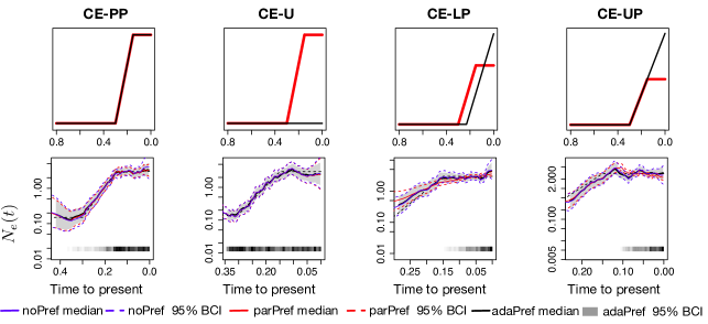
Figure 2: Simulations from constant-exponential trajectories and posterior inferences of $N_{e}(t)$. First row panels depict the simulated log-effective population size (red) and log-sampling intensity (black) trajectories (up to a constant). Second row panels depict posterior estimates for the four simulation scenarios from a single simulated genealogy picked at random with $n=500$ tips. All models used GMRF of order 1 priors and posterior inference is approximated with INLA. The posterior medians of adaPref are depicted as solid black curves and the 95% Bayesian credible regions are depicted as shaded areas. Posterior medians of parPref and noPref are depicted respectively as solid blue and red curves, and the 95% Bayesian credible regions are depicted by the corresponding dashed curves. n and s are depicted by the heat maps at the bottom of the last four panels: the squares along the time axis depict the sampling times, while the intensity of the black color depicts the number of samples. The true trajectories are depicted as a black dashed curves.

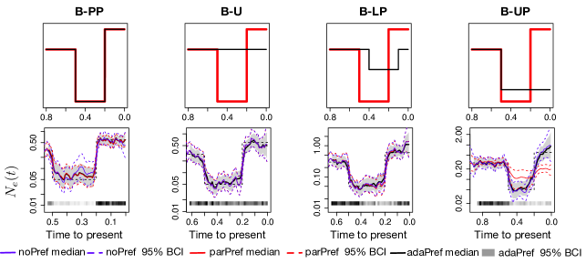
Figure 3: Simulations from bottleneck trajectories and posterior inferences of $N_{e}(t)$. First row panels depict the simulated log-effective population size (red) and log-sampling intensity (black) trajectories (up to a constant). Second row panels depict posterior estimates for the four simulation scenarios and from a single simulated genealogy picked at random with $n=500$ tips. All models used GMRF of order 1 priors and posterior inference is approximated with INLA. The posterior medians of adaPref are depicted as solid black curves and the 95% Bayesian credible regions are depicted by shaded areas. Posterior medians of parPref and noPref are depicted respectively as solid blue and red curves, and the 95% Bayesian credible regions are depicted by the corresponding dashed curves. n and s are depicted by the heat maps at the bottom of the last four panels: the squares along the time axis depict the sampling times, while the intensity of the black color depicts the number of samples. The true trajectories are depicted as a black dashed curves.

Data. We simulate genealogies under two population size trajectories: a piece-wise constant and exponential trajectory (CE), and a bottleneck trajectory (B). For the sampling protocols, we simulate sampling trajectories that resemble situations encountered in applications: a sampling protocol proportional to $N_{e}(t)$ (PP), uniform (U), a “lagged” response to changes in $N_{e}(t)$ (LP), and a situation where only some segments of the sampling trajectory are preferential (UP). The combination of the two acronyms will be used in the plots, e.g B-U refers to bottleneck trajectory and uniform sampling. The first rows of Figures 2-3 depict the $N_{e}$ (red) and $\lambda(t)$ (black) trajectories (up to a scaling constant and in log-scale) of the eight simulation scenarios considered. Exact specifics of the trajectories used are given in the supplementary material.

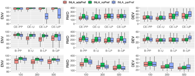
Figure 4: Summary statistics of parPref, noPref and adaPref inference of $N_{e}(t)$ approximated with INLA. In the first two rows, each box refers to one method (color in the legend) and depicts the distribution of the $150$ estimated statistics for each simulation trajectory ($50$ datasets for each sample size, $150$ in total) based on $N_{e}(t)$ posterior: ENV, first column; RWD, second column; DEV, third column. In the third row, the grouping is done according to the sample size: each box is based on $400$ simulated genealogies ($50$ genealogies for each of the eight trajectories). In the legend, INLA_adaPref is our method, INLA_noPref is the method in Palacios and Minin (2012), INLA_parPref is the method of Karcher et al. (2016). All models used GMRF of order 1 priors.

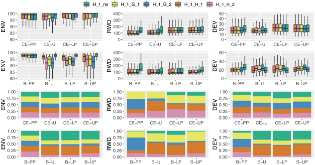
Figure 5: Summary statistics of noPref and adaPref inference of $N_{e}(t)$ on simulations with different MRF priors. In the boxplots (top two rows), each box refers to one method (color in the legend) and depicts the distribution of the $150$ estimated statistics for each simulation trajectory ($50$ datasets for each sample size, $150$ in total) based on $N_{e}(t)$ posterior: ENV, first column; RWD, second column; DEV, third column. In the stacked bar plots (bottom two rows), each bar refers to a simulation scenario and each sub-bar refers to a model (color legend). The sub-bar width represents the percentage of simulated datasets for which the model under consideration is in the top two best performance for the corresponding summary statistics ( highest ENV, lowest RWD, and lowest DEV). In the legend, the first capital letter refers to the type of prior on $N_{e}(t)$, the second one on $\beta(t)$, with H denoting the HSMR prior, G the GMRF prior; the two numbers refer to the corresponding orders.

We simulate both the coalescent times and the sampling times from their corresponding inhomogeneous Poisson processes using the Lewis-Shedler thinning algorithm (Lewis and Shedler, 1979; Palacios and Minin, 2013). We consider three sample sizes $n$ in ($100,300,500$) and $50$ simulations for each combination of trajectories and sample size. We estimated posteriors with the twenty-three models for each simulated genealogy. The code for reproducing the simulation study is available at https://github.com/lorenzocapp/adapref as a R package.

Results. We first analyze a single simulated genealogy with $n=500$ tips from each simulation scenario and approximate posterior marginals with INLA assuming GMRFs of order 1 priors. The four panels of Figure 2 second row depict the posterior medians and $95$% BCI of $N_{e}(t)$ for the constant-exponential trajectory (CE). Our adaPref results are depicted in black and grey scale, the parPref method in red, and the noPref in blue. Each column corresponds to each a sampling protocol. All posterior medians are very similar and close to the truth (black dashed line) except for parPref (red) in the last two scenarios. Indeed, the last two scenarios correspond to the cases in which the preferential sampling assumption of parPref is violated. ParPref and adaPref show similar credible region widths in the case of proportional preferential sampling (first column), however, adaPref consistently shows narrower credible regions across sampling protocols. Figure 3 shows the same type of comparisons for the bottleneck trajectory (B). The posterior median and credible intervals obtained with parPref are particularly off during the periods of no preferential sampling in the last simulation scenario (fourth column). In all other sampling scenarios, all methods have very similar posterior medians, however again, adaPref shows narrower credible regions while keeping high coverage across sampling protocols.

We now discuss the accuracy of the $N_{e}(t)$ estimators obtained with the three different models: adaPref, noPref, and parPref (approximated with INLA and using GMRF-1 priors) in the four sampling protocols for CE and B trajectories but now summarizing the estimations obtained from all 150 simulated genealogies.

Figure 4 top two rows plot the ENV, RWD, and DEV summary statistics obtained from the CE (first row) and the B (second row) trajectories. The adaPref model (red boxplots) has the best mean performance in six out of the eight scenarios in terms of both RWD and DEV (B-PP, B-U, all CE scenarios). In the last two scenarios (B-LP, B-UP), the parPref model achieved the lowest mean RWD and noPref the lowest mean DEV. Surprisingly, the adaPref model outperforms parPref also in the CE-PP and B-PP scenarios, where the parametric assumptions are met.

The adaPref model is more heavily parametrized and one may be lead to think that the performance of the adaPref estimator is affected by the sample size. Figure 4 last row panels depict the boxplots of the three statistics considered, now grouping simulations by sample size. There is no detectable sample size effect: the relative performance of the estimators is roughly similar as $n$ increases. The adaPref estimator is the best performing according to DEV and RWD averaging over all the simulation scenarios jointly.

We now assess the sensitivity of different MRF priors on $\beta(t)$ and $N_{e}(t)$ parameters in the adaPref model and compare the $N_{e}(t)$ adaPref estimators to the noPref estimators according to ENV, RWD, and DEV. We discuss the results considering the noPref model with HSMRF-1 prior on $N_{e}(t)$, the adapref models with HSMRF-1 prior on $N_{e}(t)$ and HSMRFs of orders 1 and 2, and GMRFs of orders 1 and 2, on $\beta(t)$. In all cases, we use HMC to estimate the corresponding posterior distribution. Figure 5 top two rows include the boxplots of ENV, RWD, and DEV for the eight simulation scenarios. Each bar in Figure 5 bottom two rows depicts the percentage of simulations each model was one of the top two according to ENV, RWD, and DEV across all simulation scenarios. Each bar refers to a simulation scenario according to one metric. In all plots, we include all three sample sizes considered for each simulation scenario ($1500$ data sets in total).

Results in Figure 5 confirm that modeling preferential sampling leads to better accuracy. Looking at the bottom two rows, if preferential sampling did not matter, all models would have approximately the same chance of being ranked in the top two ($20$% each). This is roughly the case for ENV in the CE scenarios. All adaPref models always achieve narrower credible regions (RWD). In terms of DEV, there are a few instances in which ignoring preferential sampling leads to better performance (B-PP, B-LP, B-UP). However, one of the adaPref models (HSMRF-1 prior on both parameters) achieves an identical performance in those scenarios. Figure 5 boxplots also show that the adaPref priors lead to narrower credible regions, and sometimes to smaller mean absolute deviations (DEV).

Although we only show results of noPref with HSMR-1 prior on $N_{e}(t)$ in Figure 5, we computed the WAIC values for the four MRF priors on $N_{e}(t)$ based on GMRF and HSMRF of orders 1 and 2. The chosen HSMR-1 model achieved the highest WAIC more frequently across the $3000$ datasets generated ($50$ runs, three sample sizes, and four sampling rates for each $N_{e}(t)$ trajectory).

5 SARS-CoV-2 in Los Angeles and Santa Clara counties

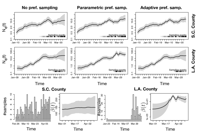
Figure 6: Phylodynamic inference with noPref, parPref and adaPref models from SARS-CoV-2 genealogies inferred from GISAID data obtained from Los Angeles and Santa Clara counties. First two rows panels depict $N_{e}(t)$ posterior distributions inferred using three possible priors: the noPref (Palacios and Minin, 2012), the parPref Karcher et al. (2016), and our adaPref prior. The last row first and third panels depict how many samples are collected each day. The second and fourth panels depict $\beta(t)$ posterior distribution (only under the adaPref prior). The posterior medians are depicted as solid black lines and the 95% Bayesian credible regions are depicted by shaded areas. Sampling times are also depicted by the heat maps at the bottom of the top two rows panels: the squares along the time axis depicts the sampling time, while the intensity of the black color depicts the number of samples.

SARS-CoV-2 is the virus responsible for the coronavirus disease pandemic in 2019-2020. Molecular surveillance of SARS-CoV-2 complements traditional surveillance methods based on case count data and provides a unique opportunity to retrospectively learn past disease dynamics. Here, we use the adaPref model for estimating the viral genetic diversity trajectory $N_{e}(t)$, from currently available viral molecular sequences in GISAID obtained from infected individuals. We analyzed viral whole-genome sequences collected in California in Santa Clara (S.C.) and Los Angeles (L.A.) counties and made publicly available in the GISAID EpiCov database (Shu and McCauley, 2017). The GISAID reference numbers of the sequences included in this study, together with data access acknowledgments, are included in the supplementary material.

We downloaded all molecular sequences available on June 27, 2020. The datasets consist of 195 and 134 sequences from S.C and L.A. counties respectively, with collection dates ranging from mid-February, 2020 to April 13 of 2020. We included only high coverage sequences with more than 25000 base pairs. Sampling frequency information is depicted in the first and third panels of the last row of Figure 6. We note that the sampling effort varied in the two counties: most of the L.A. samples are concentrated in late March-mid April, while samples have been collected throughout late February-mid April in S.C. county.

The two estimated genealogies employed in the analysis are the maximum clade credibility trees of the posterior distributions obtained with BEAST2 (Bouckaert et al., 2019). The MCMC parameters are: $20\times 10^{6}$ iterations, thinning every $1000$ and burnin of $10\times 10^{6}$ iterations. We selected the following priors: Extended Bayesian Skyline prior on $N_{e}(t)$ (Heled and Drummond, 2008), HKY mutation model with empirically estimated base frequencies (Hasegawa et al., 1985), and uniform prior on the mutation rate with support constrained between $9\times 10^{-4}$ and $1.1\times 10^{-3}$ substitutions per site per year. The support of the uniform prior was centered around $1\times 10^{-3}$ mutations per site per year, an estimate obtained by regressing the Hamming distances of the sequences to the ancestral reference sequence (GenBank MN908947, Wu et al. (2020)) on the time difference between the sampling times and the reference sampling time.

Given the two estimated genealogies, we approximate posterior marginal distributions of $N_{e}(t)$ through the INLA approximations of the noPref model (Palacios and Minin, 2012), the parPref model (Karcher et al., 2016), and our adaPref model. In the first two rows of Figure 6, we show the estimates of effective population size trajectories with the noPref model (first column), the parPref model (second column), and the adaPref model (third column). Results for S.C. county correspond to the first row and for L.A. county to the second row. Sampling intensity posteriors (computed only through the adaPref model) are given in the third row of Figure 6 in the second and third panels.

The median posteriors of $N_{e}(t)$ obtained with the noPref and the adaPref models in L.A. county have almost identical trajectories, while the one with the parPref model has a more pronounced maximum later on (around April $1$st). In the S.C. county data set, the median posterior estimates of $N_{e}(t)$ obtained with the parPref and adaPref models are in this case almost identical, with the estimate obtained with noPref not recovering a steep growth at the end of March. The split behavior of the adaPref posterior, once matching with the noPref posterior and once with parPref posterior, can be explained by looking at the posterior of $\beta(t)$: in the S.C. data set, $\beta(t)$ median posterior is practically flat, a situation consistent with the parametric assumption of the parPref model, while the time-varying $\beta(t)$ accounts for the fact that sampling in L.A. is concentrated in a short time frame. Recall that the parametric assumption of the parPref prior implies a low $N_{e}(t)$ in February and early March because there are no samples. We believe that this is a positive feature of the adaPref model that it is indeed adaptive to the different sampling protocols.

The average width of the credible regions ($RW=\frac{1}{K}\sum^{K}_{i=1}|\hat{N}_{97.5}(v_{i})-\hat{N}_{2.5}(v_{i})|$) differ across methods and datasets. In S.C. county, $RW$ is $8.5$ for noPref, $6.6$ for parPref, and $4.7$ for adaPref inferences. In L.A. county, the $RW$ is $23.9$ for noPref, $13.6$ for parPref , and $20.8$ for adaPref inferences. We get a general confirmation that preferential sampling estimators lead to narrower credible regions.

A final remark. The estimates of $N_{e}(t)$ presented here are representative of genetic diversity over time and do not directly translate to the number of infections. The coalescent we employed ignores recombination, population structure, and selection, which are all assumptions commonly violated in viruses (Rambaut et al., 2008). As more scientific knowledge on this virus is produced, the validity of our model assumptions to SARS-CoV-2 will be the subject of further research. Also, we note that observed nucleotide substitutions may be caused by sequencing errors and these are being ignored in our study.

6 Discussion

We have introduced an adaptive preferential sampling model to estimate the effective population size $N_{e}(t)$ of a coalescent process accounting for a situation in which sampling dates are stochastically dependent on the effective population size. We model sampling dates as an inhomogeneous Poisson process with rate $\beta(t)N_{e}(t)$, where $\beta(t)$ is a time-varying coefficient that modulates how this dependence varies over time. We assume that both $N_{e}(t)$ and $\beta(t)$ are continuous functions and model them in a Bayesian framework with Markov random field priors. This methodology allows us to account for preferential sampling while making minimal assumptions on the dependence between the sampling process and the genealogical process. We term the model proposed adaptive preferential sampling.

The adaptive preferential sampling model allows for a situation in which the sampling protocol changes over time but no detailed knowledge on the way samples are collected is available. In particular, the local adaptivity of the Horseshoe Markov random field prior allows also to model abrupt changes in the sampling protocol.

We show through simulation studies that the estimates obtained through the adaptive preferential sampling are more accurate than some of the available alternatives, leading to smaller absolute deviations from the true trajectories and narrower credible regions. The performance is competitive also in a broad set of scenarios in which the parametric assumptions of the alternative methods are met. We provide an application to SARS-CoV-2 monitoring and show the “adaptive nature” of our methodology: in one scenario the estimate was comparable to that of the model without preferential sampling. In a second one, the estimate was matched that of the parametric preferential sampling methodology.

The most direct extension for future work is to include genealogical uncertainty, which is being ignored in the present work. While Kingman heterochronous $n$-coalescent is the standard coalescent model choice to include genealogical uncertainty, recent works have proposed to infer $N_{e}(t)$ employing lower resolution coalescent models (Sainudiin et al., 2015; Cappello et al., 2020). Our adaptive preferential sampling framework can be paired with any of the ancestral processes.

Another natural extension to the proposed adaptive preferential framework is to incorporate covariates into $\lambda(t)$, the sampling rate, as it is done in Karcher et al. (2020), to include auxiliary information about the sampling protocols available to the modeler. For example, it is easy to imagine that one may have direct control over the sampling protocol. The resulting rate of the sampling process would be $\lambda(t)=\beta(t)N_{e}(t)+\boldsymbol{\beta}^{\prime}\textbf{X}(t)$, where X is a vector of covariates and $\boldsymbol{\beta}^{\prime}$ the corresponding linear coefficients.

In this paper, we model jointly the coalescent process and a sampling process depending on $N_{e}(t)$. An interesting direction of future work is to model jointly the coalescent process with other processes that depend on $N_{e}(t)$, such as the total number of infected individuals in an epidemic (Volz et al., 2009). The adaptive framework introduced in this paper seems to be suitable to such an extension, given that we make limited assumptions on the dependence between the two processes.

SUPPLEMENTARY MATERIAL

Observed preferential sampling of SARS-CoV-2 reported in GISAID.

Figure 7 depicts the histogram of the sampling dates of the SARS-CoV-2 USA sequences available on GISAID as of July $20$, $2020$. The red line depicts the daily number of new cases in USA (data downloaded from https://github.com/nytimes/covid-19-data).

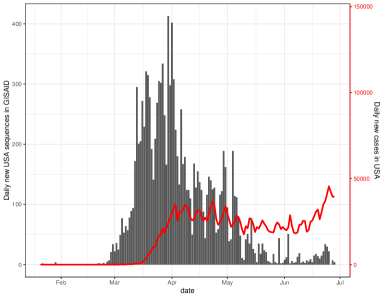
Figure 7: Sampling date of SARS-CoV-2 USA sequences available on GISAID as of July $20$, $2020$ and daily new cases in USA in the same period.

Simulation Details

We used simulations to assess the performance of the adaPref priors. We provide here details of the eight simulation trajectories considered (CE and B). In CE scenarios, $N_{e}(t)$ is equal to $3$ for $t\leq.15$, $3\exp(3-20t)$ for $.15<t\leq.3$, and $.15$ otherwise; in B scenarios, $N_{e}(t)$ is equal to $.6$ for $t\leq.2$, $.005$ for $.2<t\leq.5$, and $.3$ otherwise. The sampling rate $\lambda(t)$ changes for each simulation scenario. There is a constant of proportionality that will make it change also as a function of the sample size ($n=100,300,500$) in order to ensure that the maximum sampling times is approximately the same.

In CE-PP $\lambda(t)=c_{n}N_{e}(t)$ with $c_{n=100}=180$, $c_{n=300}=500$,$c_{n=500}=830$; in CE-U $\lambda(t)=c_{n}$ with $c_{n=100}=25$, $c_{n=300}=65$,$c_{n=500}=120$; in CE-LP $\lambda(t)=c_{n}10\exp(1.6-20t)$ for $t\leq.23$, and $c_{n}0.5$ otherwise, with $c_{n=100}=45$, $c_{n=300}=140$,$c_{n=500}=210$; in CE-UP $\lambda(t)=c_{n}10\exp(3-20t)$ for $t\leq.3$, and $c_{n}0.5$ otherwise, with $c_{n=100}=14$, $c_{n=300}=35$,$c_{n=500}=55$.

In B-PP $\lambda(t)=c_{n}N_{e}(t)$ with $c_{n=100}=520$, $c_{n=300}=1700$,$c_{n=500}=3000$; in B-U $\lambda(t)=c_{n}$ with $c_{n=100}=15$, $c_{n=300}=40$,$c_{n=500}=70$; in B-LP $\lambda(t)=c_{n}4$ for $t\leq.1$, $c_{n}2$ for $.1<t\leq.4$, and $c_{n}4$ otherwise, with $c_{n=100}=40$, $c_{n=300}=130$,$c_{n=500}=200$; in B-UP $\lambda(t)=c_{n}$ for $t\leq.5$, and $c_{n}4$ otherwise, with $c_{n=100}=150$, $c_{n=300}=210$,$c_{n=500}=250$.

Accuracy of adaPref priors in recovering $\beta(t)$.

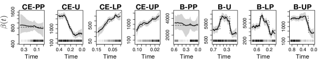
Figure 8: Posterior inferences of $\beta(t)$. Posterior estimates for the eight simulation scenarios and from a single simulated genealogy picked at random with $n=500$ tips. The posterior medians of adaPref are depicted as solid black curves and the 95% Bayesian credible regions are depicted by shaded areas. n and s are depicted by the heat maps at the bottom of the last four panels: the squares along the time axis depict the sampling times, while the intensity of the black color depicts the number of samples. True $\beta(t)$ trajectories are depicted as black dashed curves.

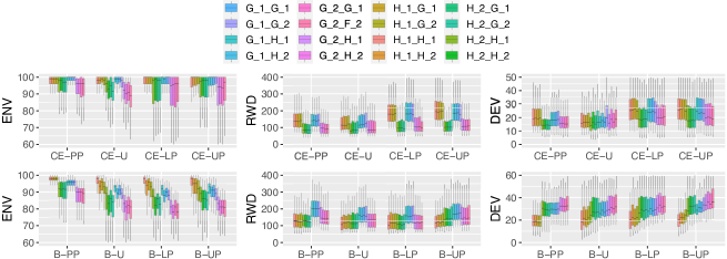
Figure 9: Summary statistics of adaPref posterior inference of $\beta(t)$ grouped by simulation study. Each box refers to one method (color in the legend) and depicts the distribution of the $150$ estimated statistics for each simulation trajectory ($50$ datasets for each sample size, $150$ in total) based on $\beta(t)$ posterior: ENV, first column; RWD, second column; DEV, third column. In the legend, the first capital letter refers to the type of prior on $N_{e}(t)$, the second one on $\beta(t)$, with H denoting the horseshoe prior, G the Gaussian prior; the two numbers refer to the corresponding orders.

We study the ability of the adaPref prior to infer the sampling intensity $\beta(t)$, which we recall to be $\lambda(t)/N_{e}(t)$. Figure 8 depicts the posterior medians and $95$% BCI of $\beta(t)$. It shows that $\beta(t)$ is well recovered in all the scenarios. Figure 9 includes the boxplots of the performance of the $16$ adaPref priors grouped by simulation scenarios. The general conclusion is that empirical accuracy is largely driven by the prior on $N_{e}(t)$: in CE, models with second-order priors on $N_{e}(t)$ (both Gaussian and Horseshoe) achieve lower RWD and DEV (boxes in shades of green and purple); in B, models with HSMRF-1 on $N_{e}(t)$ generally achieve the best performance across the three metrics. We believe that this is a positive feature of the adaPref models because the choice of the prior can be largely based on the prior on $N_{e}(t)$ which is the actual parameter of interest.

INLA posterior approximation study

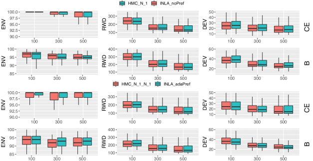
Figure 10: Summary statistics of HMC-based and INLA-based posterior inference of $N_{e}(t)$ grouped by simulation study. In the first two rows, each box refers to one method (color in the legend) and depicts the distribution of the $150$ estimated statistics for each simulation trajectory ($50$ datasets for each sample size, $150$ in total) based on $N_{e}(t)$ posterior: ENV, first column; RWD, second column; DEV, third column. In the third row, the grouping is done according to the sample size: each box is based on $400$ datasets($50$ datasets for each of the eight trajectories). In the legend, HMC_N_1_N_1 and INLA_adaPref are our methods, INLA_noPref is the method in Palacios and Minin (2012), HMC_N_1 is the method of Faulkner et al. (2020).

We continue the analysis of the simulation study discussed in Section 4. Here, we study how well INLA (Rue et al. 2009) approximates the posterior marginals of $N_{e}(t)$ across the different simulation scenarios considered and across different sample sizes ($100,300,500$). In this study we consider the HMC approximated posteriors as the “ground truth” and see how the INLA approximations perform. We compare the posteriors approximated with INLA to the ones approximated with HMC of the adaptive preferential sampling model with GMRF-1 prios on both $\beta(t)$ and $N_{e}(t)$. We do an identical comparison for the no preferential model with GMRF-1 prior on $N_{e}(t)$.

We check whether the accuracy of INLA approximated posteriors differ from that of HMC approximated posteriors. Once more, we employ ENV, RWD, and DEV to study accuracy. Figure 10 depicts the results grouped by $N_{e}(t)$ trajectory (CE, B) and sample size. The accuracies under the two approximation methods are largely comparable across simulation scenarios and sample sizes.

SARS-CoV-2 Molecular Data Description:

Data set used in the applications to SARS-CoV-2. We acknowledge the following sequence submitting laboratories to Gisaid.org:

• L.A. county data set: Cedars-Sinai Medical Center, Department of Pathology and Laboratory Medicine, Molecular Pathology Laboratory; California Department of Public Health.

• S.C. county data set: County of Santa Clara Public Health Department; County of Santa Clara Public Health; Stanford clinical virology lab; Santa Clara County Public Health Department; Chan-Zuckerberg Biohub; Chiu Laboratory, University of California, San Francisco.

We include a description of the sequences accession number and sampling date (location is determined by the county subdivision)

• L.A. county data set: $(EPI\_ISL\_4756432020-04-13),(EPI\_ISL\_4755992020-04-05),(EPI\_ISL\_4756172020-04-12),(EPI\_ISL\_4756492020-04-03),(EPI\_ISL\_4757142020-04-02),(EPI\_ISL\_4756032020-04-09),(EPI\_ISL\_4755912020-04-11),(EPI\_ISL\_4678092020-03-27),(EPI\_ISL\_4756072020-03-28),(EPI\_ISL\_4756702020-04-01),(EPI\_ISL\_4756962020-03-26),(EPI\_ISL\_4756842020-03-27),(EPI\_ISL\_4756142020-04-06),(EPI\_ISL\_4756202020-04-08),(EPI\_ISL\_4756792020-03-28),(EPI\_ISL\_4756422020-04-01),(EPI\_ISL\_4756272020-03-25),(EPI\_ISL\_4756292020-03-27),(EPI\_ISL\_4755832020-04-02),(EPI\_ISL\_4756342020-03-25),(EPI\_ISL\_4755772020-04-02),(EPI\_ISL\_4755742020-03-27),(EPI\_ISL\_4757032020-03-26),(EPI\_ISL\_4756522020-04-03),(EPI\_ISL\_4756152020-04-12),(EPI\_ISL\_4756632020-04-06),(EPI\_ISL\_4756662020-04-01),(EPI\_ISL\_4756852020-03-26),(EPI\_ISL\_4756952020-03-27),(EPI\_ISL\_4756542020-04-01),(EPI\_ISL\_4757012020-04-04),(EPI\_ISL\_4756762020-04-01),(EPI\_ISL\_4756512020-03-27),(EPI\_ISL\_4756652020-04-06),(EPI\_ISL\_4757072020-03-27),(EPI\_ISL\_4756772020-03-28),(EPI\_ISL\_4755882020-04-02),(EPI\_ISL\_4756382020-03-25),(EPI\_ISL\_4756242020-03-28),(EPI\_ISL\_4755932020-04-04),(EPI\_ISL\_4757102020-04-11),(EPI\_ISL\_4756302020-03-25),(EPI\_ISL\_4756592020-04-09),(EPI\_ISL\_4756712020-04-01),(EPI\_ISL\_4756692020-04-01),(EPI\_ISL\_4757022020-04-04),(EPI\_ISL\_4756352020-03-25),(EPI\_ISL\_4757052020-03-26),(EPI\_ISL\_4756782020-03-28),(EPI\_ISL\_4755842020-03-22),(EPI\_ISL\_4756642020-04-06),(EPI\_ISL\_4756132020-03-26),(EPI\_ISL\_4756682020-04-07),(EPI\_ISL\_4755902020-04-02),(EPI\_ISL\_4756232020-04-08),(EPI\_ISL\_4755802020-04-02),(EPI\_ISL\_4756572020-03-31),(EPI\_ISL\_4755812020-04-02),(EPI\_ISL\_4755962020-03-28),(EPI\_ISL\_4756942020-03-26),(EPI\_ISL\_4757112020-04-11),(EPI\_ISL\_4756532020-03-30),(EPI\_ISL\_4756332020-03-25),(EPI\_ISL\_4757132020-04-02),(EPI\_ISL\_4756892020-03-26),(EPI\_ISL\_4756612020-04-01),(EPI\_ISL\_4756902020-04-03),(EPI\_ISL\_4756912020-04-03),(EPI\_ISL\_4756092020-03-26),(EPI\_ISL\_4756002020-03-26),(EPI\_ISL\_4756192020-04-12),(EPI\_ISL\_4756402020-03-27),(EPI\_ISL\_4755982020-04-05),(EPI\_ISL\_4756022020-04-05),(EPI\_ISL\_4756602020-04-09),(EPI\_ISL\_4756822020-03-28),(EPI\_ISL\_4756932020-03-26),(EPI\_ISL\_4756392020-03-25),(EPI\_ISL\_4060342020-01-23),(EPI\_ISL\_4756872020-03-26),(EPI\_ISL\_4757002020-03-26),(EPI\_ISL\_4756552020-04-01),(EPI\_ISL\_4756412020-03-25),(EPI\_ISL\_4756742020-04-01),(EPI\_ISL\_4756262020-03-28),(EPI\_ISL\_4755792020-04-02),(EPI\_ISL\_4756252020-04-13),(EPI\_ISL\_4756212020-04-06),(EPI\_ISL\_4756062020-04-05),(EPI\_ISL\_4756112020-03-26),(EPI\_ISL\_4757082020-03-27),(EPI\_ISL\_4756812020-03-28),(EPI\_ISL\_4756182020-03-24),(EPI\_ISL\_4756362020-03-25),(EPI\_ISL\_4756562020-03-31),(EPI\_ISL\_4756222020-04-06),(EPI\_ISL\_4757122020-04-02),(EPI\_ISL\_4756122020-03-30),(EPI\_ISL\_4756862020-04-03),(EPI\_ISL\_4756882020-03-26),(EPI\_ISL\_4756802020-03-28),(EPI\_ISL\_4756442020-04-03),(EPI\_ISL\_4755922020-04-11),(EPI\_ISL\_4755782020-03-22),(EPI\_ISL\_4757152020-04-07),(EPI\_ISL\_4756482020-04-03),(EPI\_ISL\_4756462020-04-01),(EPI\_ISL\_4755872020-04-02),(EPI\_ISL\_4756372020-03-26),(EPI\_ISL\_4756992020-03-26),(EPI\_ISL\_4757042020-03-26),(EPI\_ISL\_4756052020-04-09),(EPI\_ISL\_4756102020-03-26),(EPI\_ISL\_4755822020-04-02),(EPI\_ISL\_4756322020-03-25),(EPI\_ISL\_4756922020-03-26),(EPI\_ISL\_4757162020-03-22),(EPI\_ISL\_4756502020-04-03),(EPI\_ISL\_4755892020-03-22),(EPI\_ISL\_4755862020-03-22),(EPI\_ISL\_4755952020-04-05),(EPI\_ISL\_4756162020-04-06),(EPI\_ISL\_4755942020-04-05),(EPI\_ISL\_4756722020-04-13),(EPI\_ISL\_4756042020-04-05),(EPI\_ISL\_4756282020-03-25),(EPI\_ISL\_4756622020-04-13),(EPI\_ISL\_4756472020-04-03),(EPI\_ISL\_4755762020-04-02),(EPI\_ISL\_4755752020-04-02),(EPI\_ISL\_4756452020-04-03),(EPI\_ISL\_4756732020-03-27),(EPI\_ISL\_4756012020-04-05),(EPI\_ISL\_4756832020-03-28),(EPI\_ISL\_4757062020-03-27),(EPI\_ISL\_4756982020-04-07),(EPI\_ISL\_4756082020-03-26),(EPI\_ISL\_4755852020-04-01),(EPI\_ISL\_4756972020-04-04),(EPI\_ISL\_4756672020-04-07),(EPI\_ISL\_4756582020-04-09),(EPI\_ISL\_4757092020-04-02),(EPI\_ISL\_4755972020-04-05),(EPI\_ISL\_4756312020-03-25),(EPI\_ISL\_4756752020-04-01)$

• S.Cla. county data set:$(EPI\_ISL\_4355992020-03-05),(EPI\_ISL\_4356012020-03-05),(EPI\_ISL\_4504552020-03-24),(EPI\_ISL\_4504562020-03-27),(EPI\_ISL\_4370762020-04-07),(EPI\_ISL\_4356152020-03-07),(EPI\_ISL\_4356272020-03-10),(EPI\_ISL\_4767872020-03-23),(EPI\_ISL\_4173172020-03-02),(EPI\_ISL\_4546682020-04-12),(EPI\_ISL\_4546582020-04-11),(EPI\_ISL\_4504602020-03-24),(EPI\_ISL\_4366472020-04-04),(EPI\_ISL\_4767892020-03-30),(EPI\_ISL\_4504682020-03-18),(EPI\_ISL\_4356542020-03-13),(EPI\_ISL\_4767782020-03-14),(EPI\_ISL\_4356492020-03-13),(EPI\_ISL\_4504582020-03-26),(EPI\_ISL\_4355972020-03-04),(EPI\_ISL\_4370582020-04-06),(EPI\_ISL\_4366462020-04-04),(EPI\_ISL\_4355872020-02-29),(EPI\_ISL\_4767722020-03-23),(EPI\_ISL\_4767912020-04-02),(EPI\_ISL\_4173182020-02-29),(EPI\_ISL\_4546842020-04-12),(EPI\_ISL\_4366722020-03-29),(EPI\_ISL\_4504762020-03-25),(EPI\_ISL\_4356392020-03-12),(EPI\_ISL\_4356532020-03-13),(EPI\_ISL\_4356602020-03-16),(EPI\_ISL\_4370552020-04-06),(EPI\_ISL\_4355902020-03-02),(EPI\_ISL\_4767862020-03-27),(EPI\_ISL\_4356702020-03-19),(EPI\_ISL\_4767802020-03-15),(EPI\_ISL\_4370462020-04-04),(EPI\_ISL\_4767682020-03-25),(EPI\_ISL\_4366592020-04-10),(EPI\_ISL\_4504462020-03-28),(EPI\_ISL\_4366422020-04-01),(EPI\_ISL\_4356572020-03-14),(EPI\_ISL\_4504672020-03-23),(EPI\_ISL\_4546862020-04-12),(EPI\_ISL\_4504452020-03-29),(EPI\_ISL\_4546672020-04-12),(EPI\_ISL\_4356362020-03-11),(EPI\_ISL\_4546792020-04-12),(EPI\_ISL\_4546732020-04-12),(EPI\_ISL\_4366442020-04-02),(EPI\_ISL\_4355802020-02-26),(EPI\_ISL\_4356082020-03-06),(EPI\_ISL\_4767822020-03-13),(EPI\_ISL\_4370492020-04-05),(EPI\_ISL\_4504752020-03-19),(EPI\_ISL\_4767932020-03-18),(EPI\_ISL\_4370642020-04-12),(EPI\_ISL\_4355982020-03-04),(EPI\_ISL\_4504642020-03-23),(EPI\_ISL\_4366772020-04-02),(EPI\_ISL\_4356092020-03-06),(EPI\_ISL\_4355812020-02-28),(EPI\_ISL\_4504742020-03-17),(EPI\_ISL\_4356412020-03-12),(EPI\_ISL\_4504492020-03-25),(EPI\_ISL\_4504662020-03-23),(EPI\_ISL\_4504652020-03-23),(EPI\_ISL\_4356472020-03-13),(EPI\_ISL\_4370522020-04-06),(EPI\_ISL\_4366602020-04-10),(EPI\_ISL\_4356402020-03-12),(EPI\_ISL\_4370572020-04-07),(EPI\_ISL\_4356002020-03-05),(EPI\_ISL\_4355962020-03-04),(EPI\_ISL\_4366542020-04-07),(EPI\_ISL\_4370652020-04-13),(EPI\_ISL\_4504622020-03-23),(EPI\_ISL\_4370852020-04-08),(EPI\_ISL\_4504702020-03-20),(EPI\_ISL\_4546552020-04-11),(EPI\_ISL\_4504792020-03-17),(EPI\_ISL\_4546542020-04-10),(EPI\_ISL\_4504512020-03-25),(EPI\_ISL\_4370452020-04-04),(EPI\_ISL\_4298792020-03-05),(EPI\_ISL\_4767852020-03-11),(EPI\_ISL\_4370432020-04-01),(EPI\_ISL\_4356302020-03-10),(EPI\_ISL\_4356122020-03-07),(EPI\_ISL\_4504772020-03-17),(EPI\_ISL\_4504722020-03-19),(EPI\_ISL\_4356212020-03-09),(EPI\_ISL\_4366612020-04-09),(EPI\_ISL\_4355862020-03-01),(EPI\_ISL\_4366762020-04-01),(EPI\_ISL\_4366672020-04-11),(EPI\_ISL\_4504522020-03-25),(EPI\_ISL\_4767832020-03-13),(EPI\_ISL\_4356712020-03-21),(EPI\_ISL\_4370842020-04-07),(EPI\_ISL\_4356192020-03-10),(EPI\_ISL\_4366652020-04-10),(EPI\_ISL\_4356372020-03-11),(EPI\_ISL\_4370472020-04-03),(EPI\_ISL\_4356312020-03-11),(EPI\_ISL\_4366552020-04-07),(EPI\_ISL\_4767942020-03-30),(EPI\_ISL\_4366562020-04-09),(EPI\_ISL\_4356502020-03-13),(EPI\_ISL\_4370802020-04-04),(EPI\_ISL\_4370482020-04-04),(EPI\_ISL\_4173202020-03-04),(EPI\_ISL\_4370782020-04-07),(EPI\_ISL\_4504732020-03-20),(EPI\_ISL\_4370872020-04-05),(EPI\_ISL\_4370832020-04-09),(EPI\_ISL\_4504802020-03-17),(EPI\_ISL\_4366662020-04-11),(EPI\_ISL\_4356282020-03-10),(EPI\_ISL\_4355822020-02-28),(EPI\_ISL\_4767812020-03-14),(EPI\_ISL\_4504482020-03-28),(EPI\_ISL\_4370502020-04-04),(EPI\_ISL\_4504782020-03-17),(EPI\_ISL\_4356612020-03-16),(EPI\_ISL\_4370772020-04-07),(EPI\_ISL\_4767922020-04-01),(EPI\_ISL\_4366822020-04-08),(EPI\_ISL\_4355942020-03-04),(EPI\_ISL\_4767732020-03-20),(EPI\_ISL\_4366782020-04-03),(EPI\_ISL\_4356182020-03-09),(EPI\_ISL\_4366692020-04-13),(EPI\_ISL\_4504612020-03-23),(EPI\_ISL\_4370512020-04-06),(EPI\_ISL\_4366742020-03-31),(EPI\_ISL\_4504572020-03-21),(EPI\_ISL\_4370592020-04-08),(EPI\_ISL\_4366522020-04-05),(EPI\_ISL\_4366812020-04-03),(EPI\_ISL\_4366452020-04-01),(EPI\_ISL\_4366752020-04-01),(EPI\_ISL\_4366802020-04-04),(EPI\_ISL\_4356382020-03-12),(EPI\_ISL\_4356432020-03-12),(EPI\_ISL\_4366532020-04-09),(EPI\_ISL\_4370562020-04-07),(EPI\_ISL\_4370532020-04-06),(EPI\_ISL\_4504542020-03-24),(EPI\_ISL\_4366482020-04-02),(EPI\_ISL\_4370632020-04-11),(EPI\_ISL\_4366572020-04-09),(EPI\_ISL\_4504592020-03-25),(EPI\_ISL\_4370612020-04-09),(EPI\_ISL\_4356622020-03-16),(EPI\_ISL\_4356582020-03-15),(EPI\_ISL\_4546742020-04-12),(EPI\_ISL\_4370442020-03-31),(EPI\_ISL\_4356452020-03-13),(EPI\_ISL\_4366642020-04-11),(EPI\_ISL\_4767752020-03-19),(EPI\_ISL\_4504692020-03-17),(EPI\_ISL\_4355832020-02-29),(EPI\_ISL\_4504812020-03-18),(EPI\_ISL\_4366632020-04-11),(EPI\_ISL\_4504632020-03-23),(EPI\_ISL\_4370542020-04-05),(EPI\_ISL\_4370862020-04-04),(EPI\_ISL\_4366732020-04-01),(EPI\_ISL\_4767882020-03-14),(EPI\_ISL\_4767792020-03-16),(EPI\_ISL\_4356662020-03-07),(EPI\_ISL\_4504712020-03-19),(EPI\_ISL\_4767842020-03-13),(EPI\_ISL\_4356512020-03-13),(EPI\_ISL\_4504472020-03-28),(EPI\_ISL\_4366432020-04-01),(EPI\_ISL\_4546532020-04-10),(EPI\_ISL\_4767902020-04-02),(EPI\_ISL\_4370882020-04-05),(EPI\_ISL\_4504532020-03-24),(EPI\_ISL\_4356342020-03-10),(EPI\_ISL\_4366792020-04-04),(EPI\_ISL\_4366502020-04-05),(EPI\_ISL\_4356332020-03-11),(EPI\_ISL\_4546702020-04-12),(EPI\_ISL\_4366622020-04-11),(EPI\_ISL\_4356632020-03-16),(EPI\_ISL\_4356672020-03-19),(EPI\_ISL\_4767742020-03-19),(EPI\_ISL\_4355852020-02-29),(EPI\_ISL\_4298802020-03-08),(EPI\_ISL\_4366512020-04-03),(EPI\_ISL\_4370622020-04-10),(EPI\_ISL\_4370602020-04-08),(EPI\_ISL\_4356352020-03-10),(EPI\_ISL\_4504502020-03-25),(EPI\_ISL\_4366412020-03-31),(EPI\_ISL\_4366582020-04-09)$

References

- (1)
- Bouckaert et al. (2019) Bouckaert, R., Vaughan, T. G., Barido-Sottani, J., Duchêne, S., Fourment, M., Gavryushkina, A., Heled, J., Jones, G., Kühnert, D., De Maio, N. et al. (2019), ‘Beast 2.5: An advanced software platform for Bayesian evolutionary analysis’, PLoS Computational Biology 15(4), e1006650.
- Cappello et al. (2020) Cappello, L., Veber, A. and Palacios, J. A. (2020), ‘The Tajima heterochronous n-coalescent: inference from heterochronously sampled molecular data’.
- Carpenter et al. (2017) Carpenter, B., Gelman, A., Hoffman, M. D., Lee, D., Goodrich, B., Betancourt, M., Brubaker, M., Guo, J., Li, P. and Riddell, A. (2017), ‘Stan: A probabilistic programming language’, Journal of Statistical Software 76(1).
- Carvalho et al. (2010) Carvalho, C. M., Polson, N. G. and Scott, J. G. (2010), ‘The horseshoe estimator for sparse signals’, Biometrika 97(2), 465–480.
- Diggle et al. (2010) Diggle, P. J., Menezes, R. and Su, T.-l. (2010), ‘Geostatistical inference under preferential sampling’, Journal of the Royal Statistical Society: Series C 59(2), 191–232.
- Drummond et al. (2005) Drummond, A. J., Rambaut, A., Shapiro, B. and Pybus, O. G. (2005), ‘Bayesian coalescent inference of past population dynamics from molecular sequences’, Molecular Biology and Evolution 22(5), 1185–1192.
- Faria et al. (2016) Faria, N. R., da Silva Azevedo, R. d. S., Kraemer, M. U., Souza, R., Cunha, M. S., Hill, S. C., Thézé, J., Bonsall, M. B., Bowden, T. A., Rissanen, I. et al. (2016), ‘Zika virus in the Americas: early epidemiological and genetic findings’, Science 352(6283), 345–349.
- Faulkner et al. (2020) Faulkner, J. R., Magee, A. F., Shapiro, B. and Minin, V. N. (2020), ‘Horseshoe-based Bayesian nonparametric estimation of effective population size trajectories’, Biometrics in press.
- Felsenstein and Rodrigo (1999) Felsenstein, J. and Rodrigo, A. G. (1999), Coalescent approaches to HIV population genetics, in ‘The Evolution of HIV’, Johns Hopkins University Press, pp. 233–272.
- Frost and Volz (2010) Frost, S. D. and Volz, E. M. (2010), ‘Viral phylodynamics and the search for an ‘effective number of infections”, Philosophical Transactions of the Royal Society B: Biological Sciences 365(1548), 1879–1890.
- Grenfell et al. (2004) Grenfell, B. T., Pybus, O. G., Gog, J. R., Wood, J. L., Daly, J. M., Mumford, J. A. and Holmes, E. C. (2004), ‘Unifying the epidemiological and evolutionary dynamics of pathogens’, Science 303(5656), 327–332.
- Hadfield et al. (2018) Hadfield, J., Megill, C., Bell, S. M., Huddleston, J., Potter, B., Callender, C., Sagulenko, P., Bedford, T. and Neher, R. A. (2018), ‘Nextstrain: real-time tracking of pathogen evolution’, Bioinformatics 34(23), 4121–4123.
- Hasegawa et al. (1985) Hasegawa, M., Kishino, H. and Yano, T. (1985), ‘Dating of the human-ape splitting by a molecular clock of mitochondrial DNA’, Journal of Molecular Evolution 2, 160–164.
- Heled and Drummond (2008) Heled, J. and Drummond, A. J. (2008), ‘Bayesian inference of population size history from multiple loci’, BMC Evolutionary Biology 8(1), 289.
- Hudson (1990) Hudson, R. R. (1990), ‘Gene genealogies and the coalescent process’, Oxford Surveys in Evolutionary Biology 7, 1–44.
- Huff et al. (2010) Huff, C. D., Xing, J., Rogers, A. R., Witherspoon, D. and Jorde, L. B. (2010), ‘Mobile elements reveal small population size in the ancient ancestors of homo sapiens’, Proceedings of the National Academy of Sciences 107(5), 2147–2152.
- Karcher et al. (2016) Karcher, M. D., Palacios, J. A., Bedford, T., Suchard, M. A. and Minin, V. N. (2016), ‘Quantifying and mitigating the effect of preferential sampling on phylodynamic inference’, PLoS Computational Biology 12(3), e1004789.
- Karcher et al. (2017) Karcher, M. D., Palacios, J. A., Lan, S. and Minin, V. N. (2017), ‘phylodyn: an R package for phylodynamic simulation and inference’, Molecular Ecology Resources 17(1), 96–100.
- Karcher et al. (2020) Karcher, M. D., Suchard, M. A., Dudas, G. and Minin, V. N. (2020), ‘Estimating effective population size changes from preferentially sampled genetic sequences’, Plos Computational Biology in press(0).
- Kim et al. (2009) Kim, S.-J., Koh, K., Boyd, S. and Gorinevsky, D. (2009), ‘ trend filtering’, SIAM Eeview 51(2), 339–360.
- Kingman (1982a) Kingman, J. F. (1982a), ‘On the genealogy of large populations’, Journal of Applied Probability 19(A), 27–43.
- Kingman (1982b) Kingman, J. F. C. (1982b), ‘The coalescent’, Stochastic Processes and their Applications 13(3), 235–248.
- Lewis and Shedler (1979) Lewis, P. W. and Shedler, G. S. (1979), ‘Simulation of nonhomogeneous Poisson processes by thinning’, Naval Research Logistics Quarterly 26(3), 403–413.
- Lorenzen et al. (2011) Lorenzen, E. D., Nogués-Bravo, D., Orlando, L., Weinstock, J., Binladen, J., Marske, K. A., Ugan, A., Borregaard, M. K., Gilbert, M. T. P., Nielsen, R. et al. (2011), ‘Species-specific responses of late quaternary megafauna to climate and humans’, Nature 479(7373), 359–364.
- Minin et al. (2008) Minin, V. N., Bloomquist, E. W. and Suchard, M. A. (2008), ‘Smooth skyride through a rough skyline: Bayesian coalescent-based inference of population dynamics’, Molecular Biology and Evolution 25(7), 1459–1471.
- Palacios and Minin (2012) Palacios, J. A. and Minin, V. N. (2012), Integrated nested Laplace approximation for Bayesian nonparametric phylodynamics, in ‘Proceedings of the Twenty-Eighth Conference on Uncertainty in Artificial Intelligence’, UAI’12, AUAI Press, Arlington, Virginia, United States, pp. 726–735.
- Palacios and Minin (2013) Palacios, J. A. and Minin, V. N. (2013), ‘Gaussian process-based Bayesian nonparametric inference of population size trajectories from gene genealogies’, Biometrics 69(1), 8–18.
- Parag et al. (2020) Parag, K. V., du Plessis, L. and Pybus, O. G. (2020), ‘Jointly inferring the dynamics of population size and sampling intensity from molecular sequences’, Molecular Biology and Evolution 37(8), 2414––2429.
- Pybus et al. (2000) Pybus, O. G., Rambaut, A. and Harvey, P. H. (2000), ‘An integrated framework for the inference of viral population history from reconstructed genealogies’, Genetics 155(3), 1429–1437.
- Rambaut et al. (2008) Rambaut, A., Pybus, O. G., Nelson, M. I., Viboud, C., Taubenberger, J. K. and Holmes, E. C. (2008), ‘The genomic and epidemiological dynamics of human influenza A virus’, Nature 453(7195), 615–619.
- Rue and Held (2005) Rue, H. and Held, L. (2005), Gaussian Markov random fields: theory and applications, CRC press.
- Rue et al. (2009) Rue, H., Martino, S. and Chopin, N. (2009), ‘Approximate Bayesian inference for latent Gaussian models by using integrated nested Laplace approximations’, Journal of the Royal Statistical Society: Series B 71(2), 319–392.
- Sainudiin et al. (2015) Sainudiin, R., Stadler, T. and Véber, A. (2015), ‘Finding the best resolution for the Kingman–Tajima coalescent: theory and applications’, Journal of Mathematical Biology 70(6), 1207–1247.
- Shapiro et al. (2004) Shapiro, B., Drummond, A. J., Rambaut, A., Wilson, M. C., Matheus, P. E., Sher, A. V., Pybus, O. G., Gilbert, M. T. P., Barnes, I., Binladen, J. et al. (2004), ‘Rise and fall of the Beringian steppe bison’, Science 306(5701), 1561–1565.
- Shu and McCauley (2017) Shu, Y. and McCauley, J. (2017), ‘GISAID: Global initiative on sharing all influenza data–from vision to reality’, Eurosurveillance 22(13), 30494.
- Slatkin and Hudson (1991) Slatkin, M. and Hudson, R. (1991), ‘Pairwise comparisons of mitochondrial DNA sequences in stable and exponentially growing populations’, Genetics 129(2), 555–562.
- Stadler (2010) Stadler, T. (2010), ‘Sampling-through-time in birth–death trees’, Journal of Theoretical Biology 267(3), 396–404.
- Stadler et al. (2013) Stadler, T., Kühnert, D., Bonhoeffer, S. and Drummond, A. J. (2013), ‘Birth–death skyline plot reveals temporal changes of epidemic spread in HIV and hepatitis C virus (HCV)’, Proceedings of the National Academy of Sciences 110(1), 228–233.
- Strimmer and Pybus (2001) Strimmer, K. and Pybus, O. G. (2001), ‘Exploring the demographic history of dna sequences using the generalized skyline plot’, Molecular Biology and Evolution 18(12), 2298–2305.
- Team et al. (2018) Team, S. D. et al. (2018), ‘Rstan: the R interface to stan. R package version 2.17. 3’.
- Vehtari et al. (2017) Vehtari, A., Gelman, A. and Gabry, J. (2017), ‘Practical Bayesian model evaluation using leave-one-out cross-validation and WAIC’, Statistics and Computing 27(5), 1413–1432.
- Volz and Frost (2014) Volz, E. M. and Frost, S. D. (2014), ‘Sampling through time and phylodynamic inference with coalescent and birth–death models’, Journal of The Royal Society Interface 11(101), 20140945.
- Volz et al. (2009) Volz, E. M., Pond, S. L. K., Ward, M. J., Brown, A. J. L. and Frost, S. D. (2009), ‘Phylodynamics of infectious disease epidemics’, Genetics 183(4), 1421–1430.
- Wakeley (2009) Wakeley, J. (2009), Coalescent theory: an introduction, Roberts and Co.
- Watanabe and Opper (2010) Watanabe, S. and Opper, M. (2010), ‘Asymptotic equivalence of Bayes cross validation and widely applicable information criterion in singular learning theory.’, Journal of Machine Learning Research 11(12).
- Wu et al. (2020) Wu, F., Zhao, S., Yu, B., Chen, Y.-M., Wang, W., Song, Z.-G., Hu, Y., Tao, Z.-W., Tian, J.-H., Pei, Y.-Y. et al. (2020), ‘A new coronavirus associated with human respiratory disease in China’, Nature 579(7798), 265–269.