Composite Estimation for Quantile Regression Kink Models with Longitudinal Data

Abstract

Kink model is developed to analyze the data where the regression function is two-stage linear but intersects at an unknown threshold. In quantile regression with longitudinal data, previous work assumed that the unknown threshold parameters or kink points are heterogeneous across different quantiles. However, the location where kink effect happens tend to be the same across different quantiles, especially in a region of neighboring quantile levels. Ignoring such homogeneity information may lead to efficiency loss for estimation. In view of this, we propose a composite estimator for the common kink point by absorbing information from multiple quantiles. In addition, we also develop a sup-likelihood-ratio test to check the kink effect at a given quantile level. A test-inversion confidence interval for the common kink point is also developed based on the quantile rank score test. The simulation study shows that the proposed composite kink estimator is more competitive with the least square estimator and the single quantile estimator. We illustrate the practical value of this work through the analysis of a body mass index and blood pressure data set.

Keywords: Quantile regression kink model, longitudinal data, composite estimation, sup-likelihood-ratio test, quantile rank score.

1 Introduction

Quantile regression, as a useful complement to mean regression, provides a systematic tool to describe the conditional distribution of a response given covariates and is more robust to outliers and heavy-tailed errors. Due to these merits, quantile regression has been extensively applied in diverse fields and also popularized in kinds of data types. One of the important data type in statistic and biostatistics is the longitudinal data, where the measurements on the same subject are repeatedly observed. So the observations within one subject are generally correlated and ignoring such correlation structure may bring statistical analysis biases. In the past two decades, a great deal of literatures have been performed to study the quantile regression for longitudinal data, see for example Koenker, (2004), Tang and Leng, (2011), Leng and Zhang, (2014), Tang et al., (2015) and Wang et al., (2019).

The literatures mentioned above always assume that the regression coefficients are constant on the whole domain of predictors. However, such stability of coefficients may be violated in some applications. For example, Li et al., (2015) studied the cognitive decline for patients with Alzheimer disease (AD) and found that cognitive function declined as normal aging in the early preclinical stage of AD and then accelerated with the progress of disease. To capture this distinctive feature, a quantile regression kink model for longitudinal data is developed in their paper. Kink regression, as a special threshold model, describes a situation where the threshold effect happens at an unknown change point in one covariate while the regression function is continuous all over the domain of predictors. Such regression has been widely applied in cross-sectional data (Li et al.,, 2011), time series data (Hansen,, 2017) and binary data (Fong et al.,, 2017), partly due to its balance between interpretability of linear model and the flexibility of nonparametric regression.

In kink models, the threshold parameter or the kink point denotes the location where the slope of a threshold predictor changes is usually of great research interest. Li et al., (2015) proposed a profiled estimation strategy to estimate model parameters by assuming that kink points are heterogeneous across different quantiles. Thus the kink points are actually estimated at each given quantile level separately. However, in some cases, the kink parameters at different quantiles, especially in neighboring quantiles tend to be the same. For example, in our empirical analysis, body mass index shows different kink effects on blood pressure at different quantiles, but the kink points appears to occur around the same location at a certain region. The estimators obtained at a single quantile may not be efficient. Although Zhang et al., (2017) studied the composite change point estimation in independent and identically distributed data, proper estimation and inference procedures for composite estimator still have not been established for longitudinal data.

In this paper, we consider a joint regression analysis of multiple quantiles for kink regression in longitudinal study. Compared to the literature, we make the following four main contributions. First, we propose a two-stage profile estimation strategy to estimate the common kink point by combining the information from different quantiles. We demonstrate that the composite estimator is more efficient than a single quantile analysis through simulation study. Second, to further check the kink effect at a given quantile, we construct a sup-likelihood-ratio test and a wild blockwise bootstrap procedures is developed to characterize the limiting distribution. Third, as the traditional Wald-type confidence interval for the kink estimator does not perform well, a test-inversion set based on the quantile rank score test in longitudinal data is developed to improve the limiting performance. Fourth, we apply the proposed composite method to the longitudinal body mass index and blood pressure data and get some interesting findings. Our method can provide a more informative analysis tool for biostatistics.

The rest of this paper is organized as follows. In Sect 2, we describe the detailed estimation procedures for the composite quantile kink regression with longitudinal data, and derive the asymptotic properties. In Sect 3, we make statistical inference on the kink estimators including the kink effect test and constructing the confidence interval. A series of simulation studies is conducted in Sect 4 to evaluate the finite sample performance of proposed methods and an application of blood pressure data analysis is illustrated in Sect 5. Sect 6 concludes this paper. The technical proofs are given in the Appendix. The R code implementing all methods is available at author’s github: https://github.com/ChuangWAN1994/CQRCPM.

2 Model and Asymptotic Property

2.1 Model setup and estimation

Suppose that we have $N$ individuals or subjects and for $i$th individual, it is measured $n_{i}$ times. So there are totally $n=\sum_{i=1}^{n}n_{i}$ observations. We denote $Y_{ij}$ as the $i$th response for $j$th individual, $X_{ij}$ as a bounded scalar covariate with thresholding effect and $\mathbf{Z}_{ij}$ as a $q$-dimensional additional covariates of interest. For any given quantile index $\tau\in(0,1)$, define the $\tau$th quantile of $Y_{ij}$ given ${\bf W}_{ij}$ as $Q_{Y}(\tau|{\bf W}_{ij})=F^{-1}(\tau|{\bf W}_{ij})=\inf\{y:F(y|{\bf W}_{ij})\}$ where ${\bf W}_{ij}=(X_{ij},\mathbf{Z}_{ij}^{\mbox{\tiny{T}}})^{\mbox{\tiny{T}}}$ and $F(\cdot|{\bf W})$ is the conditional cumulative density function of $Y$ given ${\bf W}$.

We assume that the regressor $X$ has a continuous threshold effect on the response variable $Y$ at $K$ quantile levels $0<\tau_{1}<\cdots<\tau_{K}<1$, where $K$ is a finite integer. In this paper, we are interested in the following composite quantile regression for kink model with longitudinal data:

$$\begin{array}[]{c}Q_{Y}(\tau;\boldsymbol{\eta}_{\tau_{k}},t|{\bf W}_{ij})=\alpha_{\tau_{k}}+\beta_{1,\tau_{k}}(X_{ij}-t)I(X_{ij}\leq t)+\beta_{2,\tau_{k}}(X_{ij}-t)I(X_{ij}>t)+{\bf Z}_{ij}^{\mbox{\tiny{T}}}\boldsymbol{\gamma}_{\tau_{k}}\\ \text{for $i=1,\cdots,N$; $j=1,\cdots,n_{i}$ and $k=1,\cdots,K$}\end{array}$$ (2.3)

where $\boldsymbol{\eta}_{\tau_{k}}=(\alpha_{\tau_{k}},\beta_{1,\tau_{k}},\beta_{2,\tau_{k}},\boldsymbol{\gamma}_{\tau_{k}}^{\mbox{\tiny{T}}})^{\mbox{\tiny{T}}}$ are the regression coefficients at $\tau_{k}$, $t$ is a common change point shared by $K$ baseline models with different quantile levels and $I(A)$ is an indicator function, taking 1 when $A$ is true, otherwise 0. Obviously, the slope of $X_{ij}$ equals to $\beta_{1,\tau_{k}}$ when $X_{ij}$ is less than $t$, but turns into $\beta_{2,\tau_{k}}$ for values of $X_{ij}$ greater than $t$. Meanwhile, the slopes of $\mathbf{Z}_{ij}$ stay constant on the whole domain ares. Remark that the slope of $X_{ij}$ experiences a kink at $X_{ij}=t$ while the regression function $Q_{Y}(\tau;\boldsymbol{\eta}_{\tau_{k}},t|{\bf W}_{ij})$ is everywhere continuous. Such phenomenon is generally referred to as kink effect or bent line effect. The unknown parameter $t$ is therefore called change point, kink point or other terminologies. The index set $\{\tau_{k};k=1,\cdots,K\}$ are user-specified. When $K=1$, Model (2.3) is degenerated to the standard longitudinal kink model with a kink point, which has been studied by Li et al., (2015). Here we focus on the composite estimator for the kink point $t$, which implies that the change point $t$ stays constant across $\tau_{k}$s.

Denote $\boldsymbol{\theta}=(\boldsymbol{\eta}^{\mbox{\tiny{T}}},t)^{\mbox{\tiny{T}}}$ and $\boldsymbol{\eta}=(\boldsymbol{\eta}_{\tau_{1}}^{\mbox{\tiny{T}}},\cdots,\boldsymbol{\eta}_{\tau_{k}}^{\mbox{\tiny{T}}})^{\mbox{\tiny{T}}}$. The objective function for estimating $\boldsymbol{\theta}$ is

$$S_{n}(\boldsymbol{\theta})=n^{-1}\sum_{k=1}^{K}\sum_{i=1}^{N}\sum_{j=1}^{n_{i}}\rho_{\tau_{k}}\{Y_{ij}-Q_{Y}(\tau_{k};\boldsymbol{\eta}_{\tau_{k}},t|{\bf W}_{ij})\}$$ (2.4)

where $\rho_{\tau_{k}}(v)=v\{\tau_{k}-I(v<0)\}$ is the check loss function at level $\tau_{k}$. The standard estimator for $\boldsymbol{\theta}$ is therefore given by

$$\widehat{\boldsymbol{\theta}}_{n}=\underset{\boldsymbol{\eta}\in\mathcal{B},t\in[M_{1}+\epsilon,M_{2}-\epsilon]}{\arg\min}S_{n}(\boldsymbol{\theta})$$

where $\mathcal{B}\subset\mathbb{R}^{K(q+3)}$ is a compact set for $\boldsymbol{\eta}$, $M_{1}$ and $M_{2}$ denotes the upper and lower bounds for $t$ and $\epsilon$ is a small positive number to avoid the edge effect. However, the objective function (2.4) is non-differentiable and non-smooth with respect to $t$, making the traditional convex optimization technique not applicable here. Inspired by Li et al., (2015) and Zhang et al., (2017), we adopt a two-stage profile estimation strategy to minimize (2.4). The detailed procedures go as follows:

Step 1. Note that $S_{n}(\boldsymbol{\theta})$ is linear in $\boldsymbol{\eta}$ for a given candidate $t$. So the estimator for $\boldsymbol{\eta}$ conditional on $t$ can be estimated by

$$\widehat{\boldsymbol{\eta}}_{n}(t)=\underset{\boldsymbol{\eta}\in\mathcal{B}}{\arg\min}S_{n}\{\boldsymbol{\eta}(t),t\}.$$ (2.5)

The minimization problem in (2.5) becomes a standard linear quantile regression, which can be readily implemented by some existing convex optimization packages. However, just as pointed by Zhang et al., (2017), for multiple quantiles estimation, there may exist such situation that the estimates at upper quantile levels are smaller than that at lower quantile levels, i.e. the crossing of quantile curves. Toward this end, we estimate $\boldsymbol{\eta}(t)$ by imposing a non-crossing constraint proposed by Bondell et al., (2010). One can refer to their paper for more details about the crossing issues.

Step 2. Then the change point estimator $\widehat{t}_{n}$ is given by

$$\widehat{t}_{n}=\underset{t\in[M_{1}+\epsilon,M_{2}-\epsilon]\cap(X_{n(2)},X_{n(n-1)})}{\arg\min}S_{n}\{\widehat{\boldsymbol{\eta}}_{n}(t),t\}$$ (2.6)

where $X_{n(2)}$ and $X_{n(n-1)}$ are the 2nd and $(n-1)$th order statistics of $X_{ij}$. In the specific implementation, we adopt the optimization function “optimize” in R software to solve (2.6). The ultimate estimators for $\boldsymbol{\theta}$ is therefore $\widehat{\boldsymbol{\theta}}_{n}=(\widehat{\boldsymbol{\eta}}_{n}(\widehat{t}_{n})^{\mbox{\tiny{T}}},\widehat{t}_{n})^{\mbox{\tiny{T}}}$.

2.2 Large sample properties

We now derive the asymptotic properties of $\widehat{\boldsymbol{\theta}}_{n}$. Before, we first need to introduce some notations. Define the true parameters as $\boldsymbol{\theta}_{0}=(\boldsymbol{\eta}_{0}^{\top},t_{0})^{\top}$ and $u_{ij}^{(\tau_{k})}=Y_{ij}-Q_{Y}(\tau;\boldsymbol{\eta}_{\tau_{k}},t|{\bf W}_{ij})$ as the error term with $\tau_{k}$th conditional quantile being zero. Furthermore, we define two matrixes:

$${\bf H}_{n}=n^{-1}\sum_{k=1}^{K}\sum_{l=1}^{K}\left\{\begin{array}[]{ll}\left[\sum_{i,j}\tau_{k}(1-\tau_{k}){\bf h}_{k}({\bf W}_{ij};\boldsymbol{\theta}_{0}){\bf h}_{k}({\bf W}_{ij};\boldsymbol{\theta}_{0})^{\mbox{\tiny{T}}}\right.&\\ \left.+\sum_{i}\sum_{j\neq j^{{}^{\prime}}}\left(\delta_{ijj^{{}^{\prime}}}^{(\tau_{k})}-\tau_{k}^{2}\right){\bf h}_{k}({\bf W}_{ij};\boldsymbol{\theta}_{0}){\bf h}_{k}({\bf W}_{ij^{{}^{\prime}}};\boldsymbol{\theta}_{0})^{\mbox{\tiny{T}}}\right]&(k=l)\\ &\\ \left[\sum_{i,j}(\tau_{k}\wedge\tau_{l}-\tau_{k}\tau_{l}){\bf h}_{k}({\bf W}_{ij};\boldsymbol{\theta}_{0}){\bf h}_{l}({\bf W}_{ij};\boldsymbol{\theta}_{0})^{\mbox{\tiny{T}}}\right.&\\ \left.+\sum_{i}\sum_{j\neq j^{{}^{\prime}}}\left(\xi_{ijj^{{}^{\prime}}}^{(\tau_{k})}-\tau_{k}^{2}\right){\bf h}_{k}({\bf W}_{ij};\boldsymbol{\theta}_{0}){\bf h}_{l}({\bf W}_{ij^{{}^{\prime}}};\boldsymbol{\theta}_{0})^{\mbox{\tiny{T}}}\right]&(k\neq l)\\ \end{array}\right.$$ (2.12)

where ${\bf h}_{k}({\bf W}_{ij};\boldsymbol{\theta})=({\bf 0}_{(k-1)(p+3)}^{\top},{{\bf X}}_{ij}(t)^{\top},{\bf 0}^{\top}_{(K-k)(q+3)},-\beta_{1,\tau_{k}}I(X_{ij}\leq t)-\beta_{2,\tau_{k}}I(X_{ij}>t))^{\top}$, ${{\bf X}}_{ij}(t)=(1,(X_{ij}-t)I(X_{ij}\leq t),(X_{ij}-t)I(X_{ij}>t),{\bf Z}_{ij}^{\top})^{\top}$; $\delta_{ijj^{{}^{\prime}}}^{(\tau)}=P\left(u_{ij}^{(\tau)}<0,u_{ij^{{}^{\prime}}}^{(\tau)}<0\right)$ and $\xi_{ijj^{{}^{\prime}}}^{(\tau_{k},\tau_{l})}=P\left(u_{ij}^{(\tau_{k})}<0,u_{ij}^{(\tau_{l})}<0\right)$. Define

$$\boldsymbol{\Lambda}_{n} = n^{-1}\sum_{k=1}^{K}\sum_{i=1}^{N}\sum_{j=1}^{n_{i}}\frac{\partial}{\partial\boldsymbol{\theta}}\psi_{\tau_{k}}\{Y_{ij}-Q_{Y}(\tau_{k};\boldsymbol{\eta}_{\tau_{k}},t|{\bf W}_{ij})\}{\bf h}_{k}({\bf W}_{ij};\boldsymbol{\theta})\Big{|}_{\boldsymbol{\theta}=\boldsymbol{\theta}_{0}}$$ (2.13)

$$= n^{-1}\sum_{k=1}^{K}\sum_{i=1}^{N}\sum_{j=1}^{n_{i}}f_{ij}^{(\tau_{k})}\{Q_{Y}(\tau_{k};\boldsymbol{\eta}_{\tau_{k},0},t_{0}|{\bf W}_{ij})\}{\bf h}_{k}({\bf W}_{ij};\boldsymbol{\theta}_{0}){\bf h}_{k}({\bf W}_{ij};\boldsymbol{\theta}_{0})^{\mbox{\tiny{T}}}$$

where $\psi_{\tau_{k}}(v)=\tau_{k}-I(v\leq 0)$ and $f_{ij}^{(\tau_{k})}\{Q_{Y}(\tau_{k};\boldsymbol{\eta}_{\tau_{k},0},t_{0}|{\bf W}_{ij})\}$ is the probability density function of $Y_{ij}$ given ${\bf W}_{ij}$.

We make the following necessary regularity conditions:

• The conditional distribution function $F_{ij,k}\equiv F(\tau_{k}|{\bf W}_{ij})$ has first order derivative denoted by $f_{ij}^{(\tau_{k})}(\cdot)$, which is uniformly bounded away from infinity at the point $F^{-1}(\tau_{k}|{\bf W}_{ij})$ for all $i$, $j$ and $k$. The density $f_{ij}^{(\tau_{k})}(\cdot)$ is Lipschitz continuous.

• Threshold variable $X_{ij}$ is dense in the interval $[M_{1},M_{2}]$ and has a continuous and bounded density function.

• $\max_{i,j}\|\mathbf{Z}_{ij}\|=O(n^{1/4})$ and $n^{-1}\sum_{i,j}\|\mathbf{Z}_{ij}\|^{3}=O(1)$ as $n\rightarrow\infty$.

• $\mathbf{H}_{n}\rightarrow\mathbf{H}$ and $\boldsymbol{\Lambda}_{n}\rightarrow\boldsymbol{\Lambda}$ as $n\rightarrow\infty$ where $\mathbf{H}$ and $\boldsymbol{\Lambda}$ are two positive definite matrices.

• There exists a $S(\boldsymbol{\theta})$ such that $ES_{n}(\boldsymbol{\theta})\rightarrow S(\boldsymbol{\theta})$ as $n\rightarrow\infty$, which achieves a unique global minimum at true parameters $\boldsymbol{\theta}_{0}$.

Assumption (A1) is standard in quantile regression. Assumptions (A2) and (A3) impose some conditions for threshold variable $X_{ij}$ and additional covariates $\mathbf{Z}_{ij}$, which can also be found in Li et al., (2015). Assumption (A5) ensures that the estimation is identifiable.

The following convergence result holds.

Theorem 2.1.

Suppose the Assumptions (A1)-(A4) hold and given $\beta_{1,\tau_{k}}\neq\beta_{2,\tau_{k}}$ in Model (2.3), as $n\rightarrow\infty$, $\widehat{\boldsymbol{\theta}}_{n}$ is a consistent estimator for $\boldsymbol{\theta}_{0}$ and

$$\sqrt{n}(\widehat{\boldsymbol{\theta}}_{n}-\boldsymbol{\theta}_{0})\stackrel{{\scriptstyle d}}{{\longrightarrow}}N({\textbf{0}},\boldsymbol{\Sigma})$$

where $\boldsymbol{\Sigma}=\boldsymbol{\Lambda}^{-1}{\bf H}\boldsymbol{\Lambda}^{-1}$.

Moreover, we separately estimate $\boldsymbol{\Lambda}$ and $\mathbf{H}$ by plugging in $\widehat{\boldsymbol{\Lambda}}_{n}$ and $\widehat{\mathbf{H}}_{n}$ in which

$$\widehat{\boldsymbol{\Lambda}}_{n}=\left(\begin{array}[]{cc}\widehat{\boldsymbol{\Lambda}}_{n11}&\widehat{\boldsymbol{\Lambda}}_{n12}\\ \widehat{\boldsymbol{\Lambda}}^{\top}_{n12}&\widehat{\boldsymbol{\Lambda}}_{n22}\\ \end{array}\right)$$ (2.16)

where $\widehat{\boldsymbol{\Lambda}}_{n11}=-diag(\widehat{\boldsymbol{\lambda}}_{n11,1},\cdots,\widehat{\boldsymbol{\lambda}}_{n11,K})$ is a $K(q+3)\times K(q+3)$ block diagonal matrix. For any $k=1,\cdots,K$, $\widehat{\boldsymbol{\lambda}}_{n11,k}$ is a $(q+3)\times(q+3)$ symmetric matrix given by

$$\widehat{\boldsymbol{\lambda}}_{n11,k}=n^{-1}\sum_{i=1}^{N}\sum_{j=1}^{n_{i}}\hat{f}^{(\tau_{k})}_{ij}\{Q_{Y}(\tau_{k};\widehat{\boldsymbol{\eta}}_{\tau_{k},n},\widehat{t}_{n}|{\bf W}_{ij})\}{\bf X}_{ij}(\widehat{t}_{n}){\bf X}_{ij}(\widehat{t}_{n})^{\mbox{\tiny{T}}}$$

where $\hat{f}^{(\tau)}_{ij}(\cdot)$ is a consistent estimator for $f^{(\tau)}_{ij}(\cdot)$. In practical implementation, we estimate $f_{ij}^{(\tau)}(\cdot)$ by using the difference quotient method of Hendricks and Koenker, (1992)

$$\hat{f}_{ij}^{(\tau)}\{Q_{Y}(\tau;\widehat{\boldsymbol{\eta}}_{\tau,n},\widehat{t}_{n}|{\bf W}_{ij})\}=\max\left\{0,\frac{2\Delta_{n}}{Q_{Y}(\tau+\Delta_{n};\widehat{\boldsymbol{\eta}}_{\tau,n},\widehat{t}_{n}|{\bf W}_{ij})-Q_{Y}(\tau-\Delta_{n};\widehat{\boldsymbol{\eta}}_{\tau,n},\widehat{t}_{n}|{\bf W}_{ij})}\right\}$$

where $\Delta_{n}$ is the bandwidth. We follow Hall and Sheather, (1988) and choose

$$\Delta_{n}=1.57n^{-1/3}(1.5\phi^{2}\{\Phi^{-1}(\tau)\}/[2\{\Phi^{-1}(\tau)\}^{2}+1])^{1/3}$$

where $\Phi(\cdot)$ and $\phi(\cdot)$ are the distribution and density function for standard normal distribution. In addition, $\widehat{\boldsymbol{\Lambda}}_{n12}=(\widehat{\boldsymbol{\lambda}}_{n12,1}^{\top},\cdots,\widehat{\boldsymbol{\lambda}}_{n12,K})^{\top}$ is a $K(q+3)\times 1$ vector with $k$th element

$$\widehat{\boldsymbol{\lambda}}_{n12,k}=n^{-1}\sum_{i=1}^{N}\sum_{j=1}^{n_{i}}\hat{f}_{ij}\{Q_{Y}(\tau_{k};\widehat{\boldsymbol{\theta}}_{n}|{\bf W}_{ij})\}\{\widehat{\beta}_{n,1,\tau_{k}}I(X_{ij}\leq\widehat{t}_{n})+\widehat{\beta}_{n,2,\tau_{k}}I(X_{ij}>\widehat{t}_{n})\}{\bf X}_{ij}(\widehat{t}_{n}).$$

$\widehat{\boldsymbol{\Lambda}}_{n22}$ is a scalar whose expression is $-n^{-1}\sum_{i=1}^{N}\sum_{j=1}^{n_{i}}\hat{f}_{ij}\{Q_{Y}(\tau_{k};\widehat{\boldsymbol{\theta}}_{n}|{\bf W}_{ij})\}\{\widehat{\beta}_{n,1,\tau_{k}}^{2}I(X_{ij}\leq\widehat{t}_{n})+\widehat{\beta}_{n,2,\tau_{k}}^{2}I(X_{ij}>\widehat{t}_{n})\}$.

A consistent estimator for $\mathbf{H}$ is

$$\widehat{\bf H}_{n}=n^{-1}\sum_{k=1}^{K}\sum_{l=1}^{K}\left\{\begin{array}[]{ll}\left[\sum_{i,j}\tau_{k}(1-\tau_{k}){\bf h}_{k}({\bf W}_{ij};\widehat{\boldsymbol{\theta}}_{n}){\bf h}_{k}({\bf W}_{ij};\widehat{\boldsymbol{\theta}}_{n})^{\top}\right.&\\ \left.+\sum_{i}\sum_{j\neq j^{{}^{\prime}}}\left(\widehat{\delta}_{ijj^{{}^{\prime}}}^{(\tau_{k})}-\tau_{k}^{2}\right){\bf h}_{k}({\bf W}_{ij};\widehat{\boldsymbol{\theta}}_{n}){\bf h}_{k}({\bf W}_{ij^{{}^{\prime}}};\widehat{\boldsymbol{\theta}}_{n})^{\top}\right]&(k=l)\\ &\\ \left[\sum_{i,j}(\tau_{k}\wedge\tau_{l}-\tau_{k}\tau_{l}){\bf h}_{k}({\bf W}_{ij};\widehat{\boldsymbol{\theta}}_{n}){\bf h}_{l}({\bf W}_{ij};\widehat{\boldsymbol{\theta}}_{n})^{\top}\right.&\\ \left.+\sum_{i}\sum_{j\neq j^{{}^{\prime}}}\left(\widehat{\xi}_{ijj^{{}^{\prime}}}^{(\tau_{k})}-\tau_{k}^{2}\right){\bf h}_{k}({\bf W}_{ij};\widehat{\boldsymbol{\theta}}_{n}){\bf h}_{l}({\bf W}_{ij^{{}^{\prime}}};\widehat{\boldsymbol{\theta}}_{n})^{\top}\right]&(k\neq l).\\ \end{array}\right.$$ (2.22)

One difficulty here is how to estimate $\widehat{\delta}_{ijj^{{}^{\prime}}}^{(\tau_{k})}$ and $\widehat{\xi}_{ijj^{{}^{\prime}}}^{(\tau_{k})}$ since it depends on the correlated structure within each individual. Li et al., (2015) provided four kinds of structures, they are compound symmetry, AR(1) structure, heteroscedastic correlation and unstructured correlation. We directly adopt the method of Li et al., (2015) to estimate $\widehat{\delta}_{ijj^{{}^{\prime}}}^{(\tau_{k})}$ and $\widehat{\xi}_{ijj^{{}^{\prime}}}^{(\tau_{k})}$ and omit the detailed computations for saving space.

3 Inference for Kink Point

3.1 Test for the existence of kink effect

Above parameters estimation and construction of interval are meaningful if and only if the change point significantly exists for each $\tau_{k}$, $k=1,\cdots,K$. So how to statistically test for the existence of change point for each quantile level deserves to be explored. For any quantile level $\tau\in\{\tau_{1},\cdots,\tau_{K}\}$, Li et al., (2015) defined the objective function

$$L_{n}(\boldsymbol{\eta}_{\tau},t)=n^{-1}\sum_{i=1}^{N}\sum_{j=1}^{n_{i}}\rho_{\tau}\{Y_{ij}-{\bf X}_{ij}(t)^{\mbox{\tiny{T}}}\boldsymbol{\eta}_{\tau}\}.$$ (3.1)

We are interested in the following null ($H_{0}$) and alternative ($H_{1}$) hypothesis

$$H_{0} \beta_{1,\tau}=\beta_{2,\tau} t\in\mathcal{T} H_{1}: \beta_{1,\tau}\neq\beta_{2,\tau} t\in\mathcal{T}$$: for any  v.s.  for some , (3.2)

where $\mathcal{T}$ is a compact set for $t$. Under the null hypothesis, the objective function becomes

$$\widetilde{L}_{n}=n^{-1}\sum_{i=1}^{N}\sum_{j=1}^{n_{i}}\rho_{\tau}(Y_{ij}-\widetilde{{\bf X}}_{ij}^{\mbox{\tiny{T}}}\boldsymbol{\zeta}_{\tau})$$

where $\widetilde{{\bf X}}_{ij}=(1,X_{ij},{\bf Z}_{ij}^{\mbox{\tiny{T}}})^{\mbox{\tiny{T}}}$ and $\boldsymbol{\zeta}_{\tau}=(\alpha_{\tau},\beta_{1,\tau},\boldsymbol{\gamma}_{\tau}^{\mbox{\tiny{T}}})^{\mbox{\tiny{T}}}$. In fact, $\widetilde{L}_{n}=\arg\min_{\beta_{1,\tau}=\beta_{2,\tau}}L_{n}(\boldsymbol{\eta}_{\tau},t)$. In this paper, we proposed a sup-likelihood-ratio (SLR) test for testing the existence of change point. The SLR statistics is defined as

$$SLR_{n}(\tau)=\sup_{t\in\mathcal{T}}n\left\{\widetilde{L}_{n}-L_{n}(\widehat{\boldsymbol{\eta}}_{n},\widehat{t}_{n})\right\}$$ (3.3)

To investigate the asymptotic properties of proposed SLR test statistic, we consider the following local alternative model $H_{n}$

$$Q_{Y}(\tau;\boldsymbol{\eta}_{\tau},t|{\bf W}_{ij}) = \alpha_{\tau}+\beta_{1,\tau}(X_{ij}-t)I(X_{ij}\leq t)+(\beta_{1,\tau}+n^{-1/2}\Delta\beta_{\tau})$$

$$\times(X_{ij}-t)I(X_{ij}>t)+{\bf Z}_{ij}^{\mbox{\tiny{T}}}\boldsymbol{\gamma}_{\tau}$$ (3.4)

where $\Delta\beta_{\tau}=\beta_{2,\tau}-\beta_{1,\tau}$. The following limiting results hold.

Theorem 3.1.

Under the Assumptions (A1)-(A3) and the null hypothesis $H_{0}$, $SLR_{n}(\tau)\Rightarrow(1/2)\{\sup_{t\in\mathcal{T}}\mathcal{G}(t)^{\top}{\mathcal{V}}(t)^{-1}\mathcal{G}(t)-\mathcal{G}_{1}^{\top}\mathcal{V}_{1}^{-1}\mathcal{G}_{1}\}$ in distribution as $n\rightarrow\infty$, where $\mathcal{G}(t)$ is a mean-zero Gaussian process with covariance function

$${{\bf C}}(t_{1},t_{2})=n^{-1}\left\{\sum_{i,j}{{\bf X}}_{ij}(t_{1}){{\bf X}}_{ij}(t_{2})\tau(1-\tau)+\sum_{i}\sum_{j\neq j^{{}^{\prime}}}{{\bf X}}_{ij}(t_{1}){{\bf X}}_{ij^{{}^{\prime}}}(t_{2})\left(\delta_{ijj^{{}^{\prime}}}^{(\tau)}-\tau^{2}\right)\right\},$$

and $\mathcal{V}(t)=n^{-1}\sum_{i,j}E\left\{{{\bf X}}_{ij}(t){{\bf X}}_{ij}(t)^{\top}f_{ij}\left(\widetilde{{\bf X}}_{ij}^{\top}\boldsymbol{\zeta}_{0,\tau}\right)\right\}$. $\mathcal{G}_{1}$ is also a mean-zero Gaussian process under $H_{0}$ whose covariance function is

$$\widetilde{{\bf C}}=n^{-1}\left\{\sum_{i,j}\widetilde{{\bf X}}_{ij}\widetilde{{\bf X}}_{ij}^{\top}\tau(1-\tau)+\sum_{i}\sum_{j\neq j^{{}^{\prime}}}\widetilde{{\bf X}}_{ij}\widetilde{{\bf X}}_{ij^{{}^{\prime}}}^{\top}\left(\widetilde{\delta}_{ijj^{{}^{\prime}}}^{(\tau)}-\tau^{2}\right)\right\}.$$

Theorem 3.2.

Under the Assumptions (A1)-(A3) and the local alternative model $H_{n}$, as $n\rightarrow\infty$, we have

$$SLR_{n}(\tau)\Rightarrow 1/2\left[\sup_{t\in\mathcal{T}}\left\{\mathcal{G}(t)+{\mathbf{P}}(t)\right\}^{\top}\mathcal{V}(t)^{-1}\left\{\mathcal{G}(t)+{\mathbf{P}}(t)\right\}-(\mathcal{G}_{1}+\widetilde{\mathbf{P}}_{1})^{\top}\mathcal{V}_{1}^{-1}(\mathcal{G}_{1}+\widetilde{\mathbf{P}}_{1})\right]$$

where ${\mathbf{P}}(t)=n^{-1}\sum_{i,j}{\bf X}_{ij}(t)\Delta\beta_{\tau}(X_{ij}-t)I(X_{ij}>t)f_{ij}(\widetilde{{\bf X}}_{ij}^{\top}\boldsymbol{\zeta}_{0,\tau})$ and $\widetilde{\mathbf{P}}_{1}=n^{-1}\sum_{i,j}\widetilde{{\bf X}}_{ij}\Delta\beta_{\tau}(X_{ij}-t)I(X_{ij}>t)f_{ij}(\widetilde{{\bf X}}_{ij}^{\top}\boldsymbol{\zeta}_{0,\tau})$.

From Theorems (3.1) and (3.2), if $\Delta\beta_{\tau}\neq 0$ i.e $H_{1}$ holds, ${\mathbf{P}}(t)\neq 0$ and $\widetilde{\mathbf{P}}_{1}\neq 0$. Then SLR test statistic would converge to a different limiting distribution from that under $H_{0}$. ${\mathbf{P}}(t)$ and $\widetilde{\mathbf{P}}_{1}$ here serve to distinguish the null hypothesis from the alternative hypothesis. Since the null distribution of $SLR_{n}(\tau)$ takes nonstandard form, its critical values cannot be tabulated directly. To generate the critical values, we propose a blockwise wild bootstrap method to characterize the limiting behavior of $SLR_{n}(\tau)$ under $H_{0}$. Different from the wild bootstrap method in Lee et al., (2011) and Zhang et al., (2014), we treat the observations within a subject as a block and draw disturbing sample only for the $N$ subjects, so-called blockwise bootstrap. The procedures go as follows.

  Step 1. Generate iid standard normal variable $\{u^{(b)}_{i};i=1,\cdots,N\}$ for $b=1,\cdots,B$ where $B$ is a sufficiently large positive integer.

  Step 2. Calculate the following functions, respectively

$$\mathcal{G}^{(b)}(t) =n^{-1/2}\sum_{i=1}^{N}u_{i}^{(b)}\sum_{j=1}^{n_{i}}{\bf X}_{ij}(t)\left[\tau-I\left\{Y_{ij}-{{\bf X}}_{ij}(t)^{\top}\widehat{\boldsymbol{\eta}}_{\tau}<0\right\}\right];$$

$${\mathcal{G}}_{1}^{(b)} =n^{-1/2}\sum_{i=1}^{N}u_{i}^{(b)}\sum_{j=1}^{n_{i}}\widetilde{{\bf X}}_{ij}\left\{\tau-I\left(Y_{ij}-\widetilde{{\bf X}}_{ij}^{\top}\widehat{\boldsymbol{\zeta}}_{\tau}<0\right)\right\}.$$

  Step 3. Calculate the test statistic $\{SLR_{n}^{(b)}(\tau)\}_{b=1}^{B}$:

$$SLR_{n}^{(b)}(\tau)=1/2\sup_{t\in\mathcal{T}}\left\{\mathcal{G}^{(b)}(t)^{\top}\widehat{\mathcal{V}}^{-1}\mathcal{G}^{(b)}(t)-{\mathcal{G}}_{1}^{(b)\top}\widehat{\mathcal{V}}_{1}{\mathcal{G}}_{1}^{(b)}\right\}$$

where

$$\widehat{\mathcal{V}}(t) =n^{-1}\sum_{i,j}{\bf X}_{ij}(t){\bf X}_{ij}(t)^{\top}\hat{f}_{ij}\{{\bf X}_{ij}(t)^{\top}\widehat{\boldsymbol{\eta}}_{\tau}\}$$

$$\widehat{\mathcal{V}}_{1} =n^{-1}\sum_{i,j}\widetilde{{\bf X}}_{ij}\widetilde{{\bf X}}_{ij}^{\top}\hat{f}_{ij}(\widetilde{{\bf X}}_{ij}^{\top}\widehat{\boldsymbol{\zeta}}_{\tau})$$

  Step 4. The asymptotic P-value is

$$\widehat{P}_{n}=1/B\sum_{b=1}^{B}I\left\{SLR_{n}^{(b)}(\tau)>SLR_{n}(\tau)\right\}$$

Algorithm 1   Calculate the P-values for SLR test statistic

3.2 Test-inversion confidence set for kink point

In this subsection, we propose three types of confidence intervals (CI) for the common change point. First and foremost, the Wald-type CI can be directly constructed based on the asymptotic normality in Theorem 2.1 i.e. $\widehat{t}\pm z_{\alpha/2}\text{SE}(\widehat{t})$ where $z_{\alpha/2}$ is the $\alpha/2$th upper quantile of the standard normal and $\text{SE}(\widehat{t})$ is the standard error of $\widehat{t}$ obtained by estimating $\widehat{\boldsymbol{\Sigma}}_{n}$. Secondly, the bootstrap resampling is another popular method to construct the CI. The literatures on resampling methods in quantile regression is vast but in longitudinal data, the extensively used method is the subject bootstrap. Specially, we draw data from the original subject level triples $\{(Y_{ij},X_{ij},{\bf Z}_{ij}):j=1,\cdots,n_{i}\}$ randomly with replacement for $B$ times. The bootstrap CI is defined as the $(\alpha/2)$th and $(1-\alpha/2)$th quantiles of the bootstrap estimators $\{\widehat{t}^{*}_{b},b=1,\cdots,B\}$.

The third type of CI is constructed by inversion a proposed test statistics for finding a set of null values that is not rejected at pre-specified confidence level. Therefore, we are interested in the following hypotheses

$$\text{$H_{0}:$ $t_{\tau_{k}}=t_{0}$ for all $k=1,\cdots,K$ v.s. $H_{1}$: $t_{\tau_{k}}\neq t_{0}$ for some $k$},$$ (3.5)

where $t_{0}$ is a candidate change point. The null hypothesis implies that the change points at all $K$ quantiles share a common value $t_{0}$, which exhibits homogeneity for $t$.

We build a rank score test statistic for (3.5). Under $H_{0}$, the regression coefficients $\boldsymbol{\eta}_{\tau_{k}}$ can be obtained by fitting the standard linear quantile regression with $t_{\tau_{k}}=t_{0}$. The resulting estimators are denoted as $\widehat{\boldsymbol{\eta}}_{\tau_{k}}(t_{0})$ and the corresponding residuals $\hat{u}_{ij,\tau_{k}}=Y_{ij}-Q_{Y}\{\tau_{k};\widehat{\boldsymbol{\eta}}_{\tau_{k}}(t_{0})|{\bf W}_{ij}\}$ for $k=1,\cdots,K$. Then, the first order derivative of $Q_{Y}\{\tau_{k};{\boldsymbol{\eta}}_{\tau_{k}},t|{\bf W}_{ij}\}$ w.r.t parameter $t$ evaluated at $t=t_{0}$ and ${\boldsymbol{\eta}}_{\tau_{k}}={\boldsymbol{\eta}}_{\tau_{k}}(t_{0})$ is $b_{ij}\{\tau_{k};{\boldsymbol{\eta}}_{\tau_{k}}(t_{0}),t_{0}\}=-\beta_{1,\tau_{k}}I(X_{ij}\leq t_{0})-\beta_{2,\tau_{k}}I(X_{ij}>t_{0})$.

We define the rank score test statistic as

$$RS_{n}={\bf T}_{n}^{\mbox{\tiny{T}}}\boldsymbol{\Psi}_{n}^{-1}{\bf T}_{n}$$ (3.6)

where ${\bf T}_{n}=(T_{n,1},\cdots,T_{n,K})^{\mbox{\tiny{T}}}$ is a $K\times 1$ vector with $T_{n,k}=n^{-1/2}\sum_{i=1}^{N}\sum_{j=1}^{n_{i}}b_{ij}^{*}\{\tau_{k};\widehat{\boldsymbol{\eta}}_{\tau_{k}}(t_{0}),t_{0}\}\psi_{\tau_{k}}(\hat{u}_{ij,\tau_{k}})$ and $\boldsymbol{\Psi}_{n}$ is a $K\times K$ matrix with $(k,l)$th element for $k,l=1,\cdots,K$ denoted as $\Psi_{n,k,l}$,

$$\Psi_{n,k,l}=n^{-1}\left\{\begin{array}[]{ll}\left[\sum_{i=1}^{N}\sum_{j=1}^{n_{i}}\tau_{k}(1-\tau_{k})b_{ij}^{*}\{\tau_{k};\widehat{\boldsymbol{\eta}}_{\tau_{k}}(t_{0}),t_{0}\}b_{ij}^{*}\{\tau_{l};\widehat{\boldsymbol{\eta}}_{\tau_{l}}(t_{0}),t_{0}\}+\right.&\\ \left.\sum_{i}\sum_{j\neq j^{{}^{\prime}}}\left(\delta_{ijj^{{}^{\prime}}}^{(\tau_{k})}-\tau_{k}^{2}\right)b_{ij}^{*}\{\tau_{k};\widehat{\boldsymbol{\eta}}_{\tau_{k}}(t_{0}),t_{0}\}b_{ij^{{}^{\prime}}}^{*}\{\tau_{l};\widehat{\boldsymbol{\eta}}_{\tau_{l}}(t_{0}),t_{0}\}\right]&(k=l)\\ &\\ \left[\sum_{i=1}^{N}\sum_{j=1}^{n_{i}}(\tau_{k}\wedge\tau_{l}-\tau_{k}\tau_{l})b_{ij}^{*}\{\tau_{k};\widehat{\boldsymbol{\eta}}_{\tau_{k}}(t_{0}),t_{0}\}b_{ij}^{*}\{\tau_{l};\widehat{\boldsymbol{\eta}}_{\tau_{l}}(t_{0}),t_{0}\}+\right.&\\ \left.\sum_{i}\sum_{j\neq j^{{}^{\prime}}}\left(\xi_{ijj^{{}^{\prime}}}^{(\tau_{k})}-\tau_{k}\tau_{l}\right)b_{ij}^{*}\{\tau_{k};\widehat{\boldsymbol{\eta}}_{\tau_{k}}(t_{0}),t_{0}\}b_{ij^{{}^{\prime}}}^{*}\{\tau_{l};\widehat{\boldsymbol{\eta}}_{\tau_{l}}(t_{0}),t_{0}\}\right]&(k\neq l)\\ \end{array}\right.$$ (3.12)

The $b_{ij}^{*}\{\tau_{k};\widehat{\boldsymbol{\eta}}_{\tau_{k}}(t_{0}),t_{0}\}$ is defined as follows. Let ${\bf M}(t)=({\bf X}_{11}(t),{\bf X}_{12}(t),\cdots,{\bf X}_{N,n_{N}}(t))^{\mbox{\tiny{T}}}$ be $n\times(q+3)$ matrix and ${\bf B}_{k}=(b_{11}\{\tau_{k};\widehat{\boldsymbol{\eta}}_{\tau_{k}}(t_{0}),t_{0}\},b_{12}\{\tau_{k};\widehat{\boldsymbol{\eta}}_{\tau_{k}}(t_{0}),t_{0}\},\cdots,b_{N,n_{N}}\{\tau_{k};\widehat{\boldsymbol{\eta}}_{\tau_{k}}(t_{0}),t_{0}\})^{\mbox{\tiny{T}}}$ be a $n\times 1$ vector. Furthermore, define ${\bf B}_{k}^{*}\equiv({\bf I}_{n}-{\bf V}_{k}){\bf B}_{k}$ where ${\bf I}_{n}$ is $n\times n$ identity matrix, ${\bf V}_{k}={\bf M}(t_{0})\{{\bf M}(t_{0})^{\mbox{\tiny{T}}}\boldsymbol{\Upsilon}_{k}{\bf M}(t_{0})\}^{-1}{\bf M}(t_{0})^{\mbox{\tiny{T}}}\boldsymbol{\Upsilon}_{k}$ and $\boldsymbol{\Upsilon}_{k}$ is a $n\times n$ diagonal matrix with elements $\hat{f}_{11}\{Q_{Y}(\tau_{k};\boldsymbol{\eta}_{\tau_{k},0},t_{0}|{\bf W}_{ij})\}$ for $i=1,\cdots,N$ and $j=1,\cdots,n_{i}$. So, ${\bf B}_{k}^{*}$ is actually the projection of partial score vector ${\bf B}_{k}$ on ${\bf M}(t_{0})$.

We assume the following conditions to study the asymptotic property of $RS_{n}$.

• The Lebesgue density $f_{ij}^{\tau_{k}}(\cdot)$ has a bounded first-order derivative for all $i,j$ and $k$.

• The smallest eigenvalue of $\boldsymbol{\Psi}_{n}$ is bounded away from zero as $n\rightarrow\infty$.

Assumption (A6) is an important condition in deriving the limiting behavior of rank score statistic and Assumption (A7) requires that the matrix $\boldsymbol{\Psi}_{n}$ is strictly positive definite. Both the two conditions can also be found in Zhang et al., (2017).

Theorem 3.3.

Under the Assumptions (A1)-(A4) and (A6)-(A7), and the null hypothesis $H_{0}$ in (3.5), we have $RS_{n}\stackrel{{\scriptstyle d}}{{\longrightarrow}}\chi^{2}_{K}$, as $n\rightarrow\infty$.

Based on Theorem 3.3, we develop a rank score test inversion set for the kink point and the detailed steps can be found in Algorithm 2.

  Step 1. Estimate $\widehat{t}$ by using the profiled estimation procedures in section 2.1.

  Step 2. Test $H_{0}:t=\widehat{t}+k\delta$ for $k=1,2,\cdots,$ at the significance level of 0.05 by using the proposed test statistic (3.6) where $\delta$ is a small positive increment. The upper bound is the minimum accepted point $\widehat{t}^{U}=\widehat{t}+U\delta$ for $k=U$.

  Step 3. Following the similar procedure in Step 2, we can search for the lower bound $\widehat{t}^{L}$ as the maximum accepted point. The 95% rank score test inversion CI is $[\widehat{t}^{U},\widehat{t}^{L}]$.

Algorithm 2   Rank score test inversion CI for change point

Remark 3.1.

In the special case where the error term is homoscedastic, that is, $f_{ij}^{(\tau_{k})}(\cdot)=f^{(\tau_{k})}(\cdot)$ for all $i$, $j$ and $k$, then

$${\bf V}_{k}={\bf M}(t_{0})\{{\bf M}(t_{0})^{\mbox{\tiny{T}}}{\bf M}(t_{0})\}^{-1}{\bf M}(t_{0}),$$

and the quantile rank score test does not require estimating the density $f_{ij}^{(\tau)}(\cdot)$.

4 Simulation Studies

4.1 Setup

In this section, we study the finite sample performance for the proposed methods. The simulation data were generated from the following setting

$$Y_{ij}=\alpha+\beta_{1}(X_{ij}-t)I(X_{ij}\leq t)+\beta_{2}(X_{ij}-t)I(X_{ij}>t)-\gamma Z_{ij}+e_{ij}.$$ (4.1)

where $t=5$ is the change point, $(\alpha,\beta_{1},\beta_{2},\gamma)^{\mbox{\tiny{T}}}=(3,1,-1,0.2)^{\mbox{\tiny{T}}}$ are regression coefficients and $e_{ij}$ is error term. Four different cases are considered:

Case 1. A random effect model with $e_{ij}=a_{i}+\epsilon_{ij}$ where $a_{i}\stackrel{{\scriptstyle iid}}{{\sim}}N(0,1)$ and $\epsilon_{ij}\stackrel{{\scriptstyle iid}}{{\sim}}N(0,1)$.

Case 2. An AR(1) correlation model with $e_{ij}=v(X_{ij})u_{ij}$ where $v(X_{ij})=3.2-0.2X_{ij}$, $u_{ij}=0.5u_{i,j-1}+\epsilon_{ij}$ and $\epsilon_{ij}\sim N(0,1)$.

Case 3. A heteroscedastic correlation model with $e_{ij}=a_{i}+g(X_{ij})\epsilon_{ij}$ where $a_{i}\stackrel{{\scriptstyle iid}}{{\sim}}N(0,1)$ and $g(X_{ij})=\sqrt{(3.2-0.2X_{ij})^{2}-1}$.

Case 4. A random effect model with $e_{ij}=a_{i}+\epsilon_{ij}$ where $a_{i}\stackrel{{\scriptstyle iid}}{{\sim}}N(0,1)$ and $\epsilon_{ij}\stackrel{{\scriptstyle iid}}{{\sim}}t_{3}$.

Cases 1-3 are similar to that of Li et al., (2015) and Case 4 considers the heay-tailed error. In Cases 1, 3 and 4, $X_{ij}\stackrel{{\scriptstyle iid}}{{\sim}}U(0,10)$ and in Case2, the threshold variable was generated from $X_{ij}=X_{i,j-1}+0.5$ for $j>1$ and $X_{i1}\stackrel{{\scriptstyle iid}}{{\sim}}U(0.5,7.5)$. For all cases, we let $Z_{ij}\stackrel{{\scriptstyle iid}}{{\sim}}U(0,10)$. The number of individuals is set to be $N=200$ and 400. To add imbalance for the number of subjects, we let the number of observations $n_{i}=5$ for $i=1,\cdots,N-2$ and $n_{N-1}=4$ for $(N-1)$th individual and $n_{N}=6$ for $N$th individual. Therefore, there are totally 1000 and 2000 observations respectively. For each scenario, we conduct 500 simulations.

4.2 Parameters estimation

We first evaluate the sample performance of the proposed composite quantile regression (CQR) estimator. The quantile indices are set as $\tau_{k}=k/10$ for $k=3,\cdots,7$. For comparison, we take two kinds of estimators into consideration. One is the least absolute deviation (LAD) estimator proposed by Li et al., (2015) and can be implemented by using the R code available at https://onlinelibrary.wiley.com/doi/10.1111/biom.12313, the other is the least square (LS) estimator, which is a longitudinal version of Hansen, (2017) and its implementation can be found at https://github.com/ChuangWAN1994/CQRCPM/blob/master/LSCPM.R.

Table 1 summarizes the average bias, the Monte Carlo standard deviations (SD), the estimated standard errors (ESE) and the empirical coverage probability (ECP) of 95% Wald-type confidence intervals for LAD, LS and CQR estimators of change point $t$. From the Table, all the biases are ignorable, indicating the estimated kink points of three methods are consistent. In addition, the SDs are quite close to ESEs for all methods, which illustrates the asymptotical normality for the kink estimators. For all cases, we can find that CQR estimators have smaller biases and MSEs than LAD estimators, which exhibits higher estimation efficiency. This confirms the finite sample advantages of CQR method gained by pooling information from multiple quantiles. In Case 1-3 with normal errors, the CQR and LAD estimators are comparable to that of LS estimation, but in Case 4 with heavy-tailed error, the estimators based on quantile regression (LAD and CQR) perform better than LS estimator with relatively small biases and MSEs. This phenomenon reflects the robustness advantage of quantile regression to mean regression. The coverage probabilities of Wald-type confidence intervals are generally smaller than the nominal level 95%. Although as the sample size increases to $N=400$, the coverage probabilities improves slightly. Such poor performance also appears in Li et al., (2015) and Hansen, (2017) and we will show in section 4.4 that our proposed test-inversion set based on quantile rank score can help to improve the coverage probabilities of CQR estimator.

Table 1: Simulation results of different kink point estimators. Average bias (Bias) is multiplied by a factor of 10.

Case		$N=200$			$N=400$
		LAD	LS	CQR	LAD	LS	CQR
Case 1	Bias	0.009	0.013	0.0021	-0.009	-0.013	0.005
	SD	0.118	0.096	0.106	0.084	0.065	0.072
	ESE	0.114	0.089	0.099	0.079	0.063	0.069
	MSE	0.014	0.009	0.011	0.007	0.004	0.005
	ECP	0.926	0.940	0.916	0.940	0.938	0.920
Case 2	Bias	-0.003	-0.150	-0.006	0.003	0.035	-0.002
	SD	0.247	0.195	0.224	0.191	0.148	0.147
	ESE	0.208	0.174	0.186	0.188	0.144	0.157
	MSE	0.061	0.038	0.050	0.038	0.026	0.025
	ECP	0.902	0.906	0.888	0.907	0.910	0.910
Case 3	Bias	0.028	-0.043	-0.025	-0.044	-0.040	-0.057
	SD	0.196	0.158	0.173	0.134	0.107	0.115
	ESE	0.176	0.141	0.153	0.124	0.100	0.108
	MSE	0.038	0.025	0.030	0.018	0.012	0.013
	ECP	0.914	0.920	0.892	0.918	0.930	0.930
Case 4	Bias	-0.381	-0.666	0.216	0.076	0.089	0.059
	SD	0.520	0.709	0.443	0.094	0.096	0.085
	ESE	0.387	0.447	0.336	0.089	0.088	0.078
	MSE	0.271	0.507	0.196	0.009	0.009	0.007
	ECP	0.846	0.828	0.842	0.930	0.928	0.920

4.3 Power analysis

To evaluate the Type I error and local power of proposed test in Algorithm 1, we conduct another simulation study with varying $\beta_{2}=\beta_{1}+\Delta\beta$ in model (4.1) where $\Delta\beta$ is from 0 to some values, and other parameters are kept as before. For each case, the P-values are obtained by 300 bootstrap replicates based on the sample size $n=1000$. The results are illustrated in Figure 1. As shown in the Figure, when $\Delta\beta=0$ (the lines with black circles), the powers of each case all around the nominal level 5%, suggesting that our method has reasonable control of Type I errors. As expected, as $\Delta\beta$ increases, i.e. the kink effects get strengthened, the local power across different $\tau$’s all gradually approach one. This suggests that our proposed test has decent power to detect the kink effects at different quantiles. We also observe that the powers at non-extreme quantiles such as $\tau=0.5$ are always better than extreme quantiles such as $\tau=0.1,0.9$. It is common in quantile test due to the asymmetry of observations at tail quantiles and can be improved with the sample size increases.

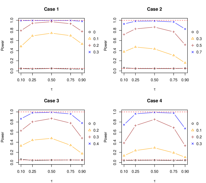
Figure 1: Power across different $\tau$’s for Case 1-4 with varying $\Delta\beta$ based on $N=200$ individuals.

4.4 Confidence intervals

Last, we evaluate the test-inversion confidence intervals based on quantile rank score (QRS) test by comparing it to the blockwise bootstrap (Boot) intervals described in Section 3.2 and the Wald-type (Wald) intrevals. The bootstrap times is set to be $400$. The estimated mean lengths (EML), the empirical coverage probabilities (ECP) and the average running time (in seconds) based on $N=200$ and $400$ of all cases are summarized in Table 2.

There is no doubt that the Wald method gives worst confidence intervals for both $N=200$ and 500 among the three constructions. In finite samples, the ECP of QRS method are, in general, more close to the nominal level than that of Boot, but the former leads relatively wider EMLs. However, QRS method costs much less computing time compared with Boot method. So it provides a good balance between the improvement of confidence interval and computational efficiency.

Table 2: Comparsion of three types of confidence intervals: Wald, Boot and QRS for $N=200$ and 400. The nominal level is 0.95.

Case	Wald			Boot			QRS
	ECP	EML	Time(s)	ECP	EML	Time(s)	ECP	EML	Time(s)
Case 1	0.916	0.445	7.060	0.942	0.419	357.590	0.958	0.591	10.580
Case 2	0.888	0.816	7.960	0.944	0.958	430.820	0.970	1.362	14.250
Case 3	0.892	0.690	7.830	0.928	0.690	400.140	0.960	1.006	14.500
Case 4	0.924	0.500	7.780	0.938	0.486	380.740	0.950	0.698	12.030
Case 1	0.930	0.311	13.240	0.948	0.385	687.150	0.954	0.401	29.400
Case 2	0.888	0.729	18.670	0.940	0.808	710.130	0.948	0.996	34.690
Case 3	0.930	0.485	15.300	0.938	0.463	780.390	0.946	0.661	26.950
Case 4	0.922	0.347	13.100	0.928	0.324	740.060	0.948	0.470	35.610

5 Analysis of Blood Pressure and Body Mass Index

It is well known that blood pressure is an important indicator for human’s health. In chronic epidemiology, high blood pressure may lead to kinds of health problems such as coronary heart disease and stroke, while low blood pressure will cause a shortage of blood to the body’s organs and then some symptoms such as the dizziness, the limb movement disorder are appeared. One important topic in public health field is to study the relationship between the blood pressure (BP) and body mass index (BMI). Previous literatures suggested that BMI shows positive association with BP (He et al., (1994), Tesfaye et al., (2007)), but some researcher found that the linear models are not sufficient to capture the positive relationship between BMI and BP. For instances, Kerry et al., (2005) showed that there presents an significant nonlinear effect between BMI and diastolic BP for young women. Zhang et al., (2014) formally demonstrated the existence of quantile threshold effect of BMI on systolic BP by using quantile score test statistic. Moreover, Zhang et al., (2017) studied the composite estimation for change point across different quantiles between BMI and systolic BP by analyzing the data from the National Health and Nutrition Examination Survey (NHAENES).

In this section, we analyze a BMI and systolic BP longitudinal data from the Nation Growth , Lung and Health Study (NGHS), avaiable at the NIH BioLINCC site (https://biolincc.nhlbi.nih.gov/). The NGHS is a multi-center population-based cohort study conducted to evaluate the longitudinal changes of childhood cardiovascular risk factors for 1166 Caucasian and 1213 African American girls. We only draw a subset of the first 300 subjects at the ages from 9 to 19. After removing some missing values, there are totally 2455 observations. Different from the previous analysis , we examine the impacts of BMI on BP by using the proposed methods to account for the dependence within one subject. Three quantile indices sets are considered, including lower quantiles (LQ) set $\{0.27,0.28,0.29,\cdots,0.33\}$, median quantiles set (MQ) $\{0.48,0.49,0.50,0.51,0.52\}$ and high quantiles set $\{0.77,0.78,0.79,\cdots,0.83\}$.

We first examine the existence of BMI kink effect by employing the proposed SLR test procedures in Algorithm 1 in Section 3.2 at each quantile level. The results of P-values and estimated kink point estimators are reported in Table 3. From the table, we observe that all the P-values approach zeros, suggesting significant kink effects at all quantiles. The kink estimators are quite close within one indices set. To further check the commonality of kink points, we consider the following hypotheses

$$\text{$H_{0}:$ $t_{\tau_{1}}=\cdots=t_{\tau_{K}}$\quad v.s.\quad$H_{1}$: $t_{\tau_{k}}\neq t_{\tau_{l}}$ for some $k\neq l$}.$$ (5.1)

For testing (5.1), we can construct the Wald type statistic based on the asymptotic properties in Li et al., (2015). The resulting P-values for LQ, MQ and HQ are 0.101, 0.075 and 0.987, respectively, confirming the statistical existence of common kink points at the significance level 5%. To capture poential kink effects, we have the following longitudinal quantile regression model at a given $\tau$

$$Q_{Y}(\tau|X_{ij},Z_{ij})=\alpha_{\tau}+\beta_{1,\tau}(X_{ij}-t)I(X_{ij}\leq t)+\beta_{2,\tau}I(X_{ij}>t)+\gamma_{\tau}Z_{ij},$$

where $X_{ij}$ and $Z_{ij}$ denote BMI and the age, respectively. $(\alpha_{\tau},\beta_{1,\tau},\beta_{2,\tau},\gamma_{\tau})^{\mbox{\tiny{T}}}$ are unknown regression coefficients varying with $\tau$ and $t$ is unknown change point that are common within one indices set. By using the two-step estimation method described in Section 2.1, we can obtain the coefficients estimators across different $\tau$’s and the composite change point estimator. Table 4 summarizes the estimation results and the different types of confidence intervals of LS, LAD and CQR methods. For CQR method, we only report the results of $\tau=0.3$ for LQ, $\tau=0.5$ for MQ and $\tau=0.8$ for HQ.

Table 3: P-values of sup-likelihood-ratio test and the kink point estimators for LQ, MQ and HQ.

	LQ			MQ			HQ
$\tau$	SLR	$\widehat{t}_{\tau}$	$\tau$	SLR	$\widehat{t}_{\tau}$	$\tau$	SLR	$\widehat{t}_{\tau}$
0.27	0.005	26.335	0.48	0.000	28.441	0.77	0.005	29.246
0.28	0.000	28.087	0.49	0.000	28.350	0.78	0.000	29.069
0.29	0.005	26.750	0.50	0.000	28.461	0.79	0.005	29.123
0.30	0.000	26.044	0.51	0.000	28.414	0.80	0.015	29.027
0.31	0.000	27.856	0.52	0.000	28.484	0.81	0.015	29.022
0.32	0.000	27.857				0.82	0.020	29.027
0.33	0.000	28.179				0.83	0.015	29.022

From the Table 4, the coefficients show that systolic BP firstly increases with BMI ($\beta_{1}>0$ of all methods), but with BMI reaching centain kink points, the positive growth relationship gets weaker ($\beta_{2}<\beta_{1}$). The estimated $\gamma$ all greater than zeros indicates a positively effect of age on systolic BP. This finding in accordance with Zhang et al., (2014) and Zhang et al., (2017). For different methods, the kink point estimators are different. For LS estimators, it models the conditional mean of systolic BP and the estimated kink point is around 26.225 kg/m². The LAD method is a single quantile analysis given by Li et al., (2015). Interestingly, we find that as $\tau$ increases, the estimated kink points increase from 26.004 kg/m² to 29.027 kg/m². Such phenomenon also appears in composite estimator whose kink estimators are 26.045 kg/m², 28.461 kg/m² and 29.069 kg/m² for LH, MQ and HQ respectively. This truth has a biological intuition that people with high BP are more likely to possess higher BMIs, therefore reaching the turning point later. Compared with LAD method, the proposed composite estimation gives shorter confidence intervals for the kink points, which indicates that combining information from multiple quantiles leads to more efficient estimation than only using a single quantile information. The fitted quantile curves of BMI against systolic BP at LQ, MQ and HQ in Figure 2 also illustrates our empirical findings.

Table 4: The estimated parameters, the standard errors (listed in parentheses) and the their confidence intervals from different estimating methods

	LS		LAD			CQR
		0.3	0.5	0.8	LQ	MQ	HQ
$\alpha$	$\mathop{103.986}\limits_{(1.926)}$	$\mathop{99.437}\limits_{(2.961)}$	$\mathop{105.130}\limits_{(1.415)}$	$\mathop{112.546}\limits_{(2.063)}$	$\mathop{99.524}\limits_{(1.705)}$	$\mathop{105.627}\limits_{(1.189)}$	$\mathop{112.504}\limits_{(1.362)}$
Wald	[100.211,107.760]	[93.621,105.253]	[102.357,107.903]	[108.497,116.595]	[96.182,102.865]	[102.850,107.510]	[109.835,115.174]
Boot	[98.019,108.054]	[93.248,103.672]	[97.768,110.080]	[106.958,120.005]	[94.214,103.791]	[98.359,109.340]	[105.697,119.221]
$\beta_{1}$	$\mathop{0.971}\limits_{(0.121)}$	$\mathop{1.059}\limits_{(0.013)}$	$\mathop{0.924}\limits_{(0.004)}$	$\mathop{0.815}\limits_{(0.017)}$	$\mathop{1.060}\limits_{(0.116)}$	$\mathop{0.928}\limits_{(0.066)}$	$\mathop{0.814}\limits_{(0.127)}$
Wald	[0.733,1.208]	[1.033,1.084]	[0.916,0.933]	[0.783,0.847]	[0.833,1.286]	[0.798,1.058]	[0.566,1.062]
Boot	[0.763,2.051]	[0.805,1.946]	[0.722,1.922]	[0.528,1.239]	[0.820,1.933]	[0.719,2.169]	[0.528,2.040]
$\beta_{2}$	$\mathop{0.239}\limits_{(0.142)}$	$\mathop{0.218}\limits_{(0.007)}$	$\mathop{0.145}\limits_{(0.076)}$	$\mathop{0.115}\limits_{(0.014)}$	$\mathop{0.217}\limits_{(0.082)}$	$\mathop{0.141}\limits_{(0.276)}$	$\mathop{0.101}\limits_{(0.114)}$
Wald	[-0.039,0.518]	[0.204,0.231]	[-0.005,0.294]	[0.088,0.142]	[0.057,0.378]	[-0.401,0.682]	[-0.122,0.324]
Boot	[-0.101,0.594]	[-0.047,0.579]	[-0.109,0.625]	[-0.849,2.834]	[-0.041,0.498]	[-0.225,0.562]	[-0.750,2.138]
$\gamma$	$\mathop{0.421}\limits_{(0.088)}$	$\mathop{0.446}\limits_{(0.006)}$	$\mathop{0.433}\limits_{(0.005)}$	$\mathop{0.404}\limits_{(0.009)}$	$\mathop{0.441}\limits_{(0.076)}$	$\mathop{0.429}\limits_{(0.073)}$	$\mathop{0.410}\limits_{(0.093)}$
Wald	[0.249,0.593]	[0.435,0.458]	[0.422,0.443]	[0.387,0.422]	[0.292,0.591]	[0.286,0.571]	[0.228,0.592]
Boot	[0.256,0.604]	[0.269,0.624]	[0.211,0.621]	[0.166,0.652]	[0.246,0.623]	[0.187,0.590]	[0.180,0.639]
$t$	$\mathop{26.225}\limits_{(1.339)}$	$\mathop{26.044}\limits_{(0.446)}$	$\mathop{28.414}\limits_{(0.822)}$	$\mathop{29.027}\limits_{(4.215)}$	$\mathop{26.045}\limits_{(1.297)}$	$\mathop{28.461}\limits_{(0.625)}$	$\mathop{29.069}\limits_{(1.947)}$
Wald	[23.601,28.849]	[22.891,29.197]	[26.803,30.024]	[20.767,37.288]	[23.502,28.587]	[27.236,29.687]	[25.252,32.886]
Boot	[18.875,29.613]	[19.632,29.515]	[19.732,33.626]	[18.416,43.727]	[19.666,29.732]	[19.842,33.428]	[23.540,43.754]
Score					[19.040,29.936]	[25.456,31.372]	[23.227,38.416]

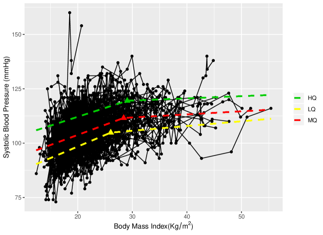
Figure 2: The fitted quantile curves at different quantile levels for BMI against systolic BP. $\blacktriangle$ denotes the estimated kink points.

6 Discussion

To aggregate the common kink point information from multiple quantiles, we proposed a new composite estimation method for kink quantile regression in longitudinal data. Compared with the method in Li et al., (2015), the proposed method can effectively capture the common kink effect. Both the simulation study and empirical analysis demonstrate that the composite estimating method is competitively efficient with the least square method and single quantile estimation method while more robust for heavy-tailed errors.

In this paper, to obtain composite estimator, we first find a index set including multiple quantiles and then verify its commonality. In reality, it is hard to find such quantile index set. Instead, it is more often that the neighbouring quantiles shares the same kink point but at different regional quantile, the kink points are different. To solve this issue, a direct approach may adopt the regularization method and the objective function becomes

$$S_{n}(\boldsymbol{\theta})=n^{-1}\sum_{k=1}^{K}\sum_{i=1}^{N}\sum_{j=1}^{n_{i}}\rho_{\tau}\{Y_{ij}-Q_{Y}(\tau_{k};\boldsymbol{\eta}_{\tau_{k}},t_{\tau_{k}}|{\bf W}_{ij})\}+\sum_{k=2}^{K}p_{\lambda}(|t_{\tau_{k}}-t_{\tau_{k-1}}|)$$

where $p_{\lambda}(\cdot)$ is some penalty function such as LASSO (Tibshirani,, 1996) and SCAD (Fan and Li,, 2001). Reseach in this direction needs further investigation.

APPENDIX

A.1 Proof of Theorem 2.1:

Lemma A.1.

(Consistency) under Assumptions (A1)-(A3) and (A5), $\widehat{\boldsymbol{\theta}}$ is a strongly consistent estimator of $\boldsymbol{\theta}_{0}$ as $n\rightarrow\infty$,

Proof of Lemma A.1: The proof of this lemma is essentially the same as that in Theorem 1 of Li et al., (2015). Note that for a fixed $t$, the objective function is $S_{n}(\boldsymbol{\theta})$, which is equivalent to minimize

$$n^{-1}\sum_{i=1}^{N}\sum_{j=1}^{n_{i}}\rho_{\tau_{k}}\{Y_{ij}-Q_{Y}(\tau_{k};\boldsymbol{\eta}_{\tau_{k}}(t),t|{\bf W}_{ij})\},$$

for each $k=1,\cdots,K$. The rest of the proof shares the similar arguments in Theorem 1 of Li (2015). One can refer to their paper for more details and thus is omited here. $\hfill\blacksquare$

Lemma A.2.

Define

$$u_{i}(\boldsymbol{\theta},\boldsymbol{\theta}_{0})= \sum_{k=1}^{K}\sum_{j=1}^{n_{i}}\psi_{\tau_{k}}\{Y_{ij}-Q_{Y}(\tau_{k};\boldsymbol{\eta}_{\tau_{k}},t|{\bf W}_{ij})\}h_{k}({\bf W}_{ij};\boldsymbol{\theta})$$

$$-\sum_{k=1}^{K}\sum_{j=1}^{n_{i}}\psi_{\tau_{k}}\{Y_{ij}-Q_{Y}(\tau_{k};\boldsymbol{\eta}_{\tau_{k},0},t_{0}|{\bf W}_{ij})\}h_{k}({\bf W}_{ij};\boldsymbol{\theta}_{0})$$

Suppose that the Assumptions (A1)-(A3) hold, then the following equation holds

$$\sup_{\|\boldsymbol{\theta}-\boldsymbol{\theta}_{0}\|\leq dn^{-1/2}}n^{-1/2}\Big{\|}\sum_{i=1}^{N}\left\{u_{i}(\boldsymbol{\theta},\boldsymbol{\theta}_{0})-E[u_{i}(\boldsymbol{\theta},\boldsymbol{\theta}_{0})]\right\}\Big{\|}=o_{p}(1)$$ (A.1)

where $d$ is some positive constant.

Proof of Lemma A.2: By using the same argument in Theorem 2 of Li et al., (2015), it is easy to show that

$$\sum_{k=1}^{K}\sum_{i=1}^{N}\sum_{j=1}^{n_{i}}\psi_{\tau_{k}}\{Y_{ij}-Q_{Y}(\tau;\widehat{\boldsymbol{\eta}}_{\tau_{k}},\widehat{t}|{\bf W}_{ij})\}h_{k}({\bf W}_{ij};\widehat{\boldsymbol{\theta}})=o(n^{1/4}\left(\log\log n)^{1/2}\right)\quad\text{a.s.}$$ (A.2)

Based on (A.2), Lemma (A.2) can be established directly by Theorem 2.2 of He and Shao, (1996) if the required conditions in that theorem hold. Thus it is sufficient to verify the conditions (B1)-(B4) and (B5${}^{{}^{\prime}}$) of He and Shao, (1996).

For (B1), the measurability is directly satisfied.

For (B2), this can be obtained from the strong consistency in Lemma A.1.

To verify (B3), we partition $u_{i}(\boldsymbol{\theta},\boldsymbol{\theta}_{0})$ based on the value of $X_{ij}$ such that

$$U_{i}(\boldsymbol{\theta},\boldsymbol{\theta}_{0})$$

$$= \sum_{k=1}^{K}\sum_{j=1}^{n_{i}}\Big{[}\psi_{\tau_{k}}\{Y_{ij}-Q_{Y}(\tau_{k};\boldsymbol{\eta}_{\tau_{k}},t|{\bf W}_{ij})\}h_{k}({\bf W}_{ij};\boldsymbol{\theta})-\psi_{\tau_{k}}\{Y_{ij}-Q_{Y}(\tau_{k};\boldsymbol{\eta}_{\tau_{k},0},t_{0}|{\bf W}_{ij})\}h_{k}({\bf W}_{ij};\boldsymbol{\theta}_{0})\Big{]}$$

$$\times I\{X_{ij}>\max(t,t_{0})\}+\sum_{k=1}^{K}\sum_{j=1}^{n_{i}}\Big{[}\psi_{\tau_{k}}\{Y_{ij}-Q_{Y}(\tau_{k};\boldsymbol{\eta}_{\tau_{k}},t|{\bf W}_{ij})\}h_{k}({\bf W}_{ij};\boldsymbol{\theta})-\psi_{\tau_{k}}\{Y_{ij}-$$

$$Q_{Y}(\tau_{k};\boldsymbol{\eta}_{\tau_{k},0},t_{0}|{\bf W}_{ij})\}h_{k}({\bf W}_{ij};\boldsymbol{\theta}_{0})\Big{]}I\{t<X_{ij}\leq t_{0}\}+\sum_{k=1}^{K}\sum_{j=1}^{n_{i}}\Big{\{}\psi_{\tau_{k}}\{Y_{ij}-Q_{Y}(\tau_{k};\boldsymbol{\eta}_{\tau_{k}},t|{\bf W}_{ij})\}$$

$$\times h_{k}({\bf W}_{ij};\boldsymbol{\theta})-\psi_{\tau_{k}}\{Y_{ij}-Q_{Y}(\tau_{k};\boldsymbol{\eta}_{\tau_{k},0},t_{0}|{\bf W}_{ij})\}h_{k}({\bf W}_{ij};\boldsymbol{\theta}_{0})\Big{\}}I\{t_{0}<X_{ij}\leq t\}+\sum_{k=1}^{K}\sum_{j=1}^{n_{i}}\Big{[}$$

$$\psi_{\tau_{k}}\{Y_{ij}-Q_{Y}(\tau_{k};\boldsymbol{\eta}_{\tau_{k}},t|{\bf W}_{ij})\}h_{k}({\bf W}_{ij};\boldsymbol{\theta})-\psi_{\tau_{k}}\{Y_{ij}-Q_{Y}(\tau_{k};\boldsymbol{\eta}_{\tau_{k},0},t_{0}|{\bf W}_{ij})\}h_{k}({\bf W}_{ij};\boldsymbol{\theta}_{0})\Big{]}$$

$$\times I\{X_{ij}\leq\min(t,t_{0})\}$$

$$\equiv U_{i1}(\boldsymbol{\theta},\boldsymbol{\theta}_{0})+U_{i2}(\boldsymbol{\theta},\boldsymbol{\theta}_{0})+U_{i3}(\boldsymbol{\theta},\boldsymbol{\theta}_{0})+U_{i4}(\boldsymbol{\theta},\boldsymbol{\theta}_{0}).$$

Then it is sufficient to show

$$\sup_{\|\boldsymbol{\theta}-\boldsymbol{\theta}_{0}\|\leq dn^{-1/2}}\Big{\|}n^{-1/2}\sum_{i=1}^{N}\{U_{ij}(\boldsymbol{\theta},\boldsymbol{\theta}_{0})-E[U_{ij}(\boldsymbol{\theta},\boldsymbol{\theta}_{0})]\}\Big{\|}=o_{p}(1)$$

for $j=1,2,3,4$. For any $\|\boldsymbol{\theta}-\boldsymbol{\theta}_{0}\|\leq dn^{1/2}$, we have

$$\|U_{i1}(\boldsymbol{\theta},\boldsymbol{\theta}_{0})\|$$

$$= \Big{\|}\Big{[}\sum_{k=1}^{K}\sum_{j=1}^{n_{i}}\psi_{\tau_{k}}\{Y_{ij}-Q_{Y}(\tau_{k};\boldsymbol{\eta}_{\tau_{k}},t|{\bf W}_{ij})\}h_{k}({\bf W}_{ij};\boldsymbol{\theta})-\sum_{k=1}^{K}\sum_{j=1}^{n_{i}}\psi_{\tau_{k}}\{Y_{ij}-Q_{Y}(\tau_{k};\boldsymbol{\eta}_{\tau_{k},0},t_{0}|{\bf W}_{ij})\}$$

$$\times h_{k}({\bf W}_{ij};\boldsymbol{\theta}_{0})\Big{]}I\{X_{ij}>\max(t,t_{0})\}\Big{\|}$$

$$\leq \Big{\|}\sum_{k=1}^{K}\sum_{j=1}^{n_{i}}\psi_{\tau_{k}}\{Y_{ij}-Q_{Y}(\tau_{k};\boldsymbol{\eta}_{\tau_{k}},t|{\bf W}_{ij})\}\{h_{k}({\bf W}_{ij};\boldsymbol{\theta})-h_{k}({\bf W}_{ij};\boldsymbol{\theta}_{0})\}I\{X_{ij}>\max(t,t_{0})\}\Big{\|}$$

$$+\Big{\|}\sum_{k=1}^{K}\sum_{j=1}^{n_{i}}\left[\psi_{\tau_{k}}\{Y_{ij}-Q_{Y}(\tau_{k};\boldsymbol{\eta}_{\tau_{k}},t|{\bf W}_{ij})\}-\psi_{\tau_{k}}\{Y_{ij}-Q_{Y}(\tau_{k};\boldsymbol{\eta}_{\tau_{k},0},t_{0}|{\bf W}_{ij})\}\right]h_{k}({\bf W}_{ij};\boldsymbol{\theta}_{0})$$

$$\times I\{X_{ij}>\max(t,t_{0})\}\Big{\|}$$

$$\equiv \|I_{i1}\|+\|I_{i2}\|$$

For $I_{i1}$, it is obvious that $E(\|I_{i1}\|^{2}|{\bf W}_{ij})=o_{p}(1)$. For $I_{2i}$, we have

$$\|I_{i2}\| \leq C_{1}\sum_{k=1}^{K}\sum_{j=1}^{n_{i}}\|{\bf U}_{ij}\|I\{Q_{1}(\tau_{k};\boldsymbol{\theta},\boldsymbol{\theta}_{0})\leq Y_{ij}\leq Q_{2}(\tau_{k};\boldsymbol{\theta},\boldsymbol{\theta}_{0})\}I\{X_{ij}>\max(t,t_{0})\}$$

where $C_{1}$ is some positive constant, ${\bf U}_{ij}=(1,X_{ij},{\bf Z}_{ij}^{\mbox{\tiny{T}}})^{\mbox{\tiny{T}}}$, $Q_{1}(\tau_{k};\boldsymbol{\theta},\boldsymbol{\theta}_{0})$ and $Q_{2}(\tau_{k};\boldsymbol{\theta},\boldsymbol{\theta}_{0})$ denote the minimum and maximum values between $Q_{Y}(\tau_{k};\boldsymbol{\eta}_{\tau_{k}},t|{\bf W}_{ij})$ and $Q_{Y}(\tau_{k};\boldsymbol{\eta}_{\tau_{k},0},t_{0}|{\bf W}_{ij})$. Thus

$$E(\|I_{i2}\|^{2}|{\bf W}_{ij})$$

$$\leq C_{1}^{2}\sum_{j=1}^{n_{i}}\Big{[}\|{\bf U}_{ij}\|^{2}I\{X_{ij}>\max(t,t_{0})\}\Big{]}E\Big{[}\sum_{k=1}^{K}\sum_{l=1}^{K}I\{Q_{1}(\tau_{k};\boldsymbol{\theta},\boldsymbol{\theta}_{0})\leq Y_{ij}\leq Q_{2}(\tau_{k};\boldsymbol{\theta},\boldsymbol{\theta}_{0})\}$$

$$\times I\{Q_{1}(\tau_{l};\boldsymbol{\theta},\boldsymbol{\theta}_{0})\leq Y_{ij}\leq Q_{2}(\tau_{l};\boldsymbol{\theta},\boldsymbol{\theta}_{0})\}\Big{]}.$$

Without loss of generality, we assume $\max\{Q_{1}(\tau_{k};\boldsymbol{\theta},\boldsymbol{\theta}_{0}),Q_{1}(\tau_{l};\boldsymbol{\theta},\boldsymbol{\theta}_{0})\}\leq\min\{Q_{2}(\tau_{k};\boldsymbol{\theta},\boldsymbol{\theta}_{0}),Q_{1}(\tau_{l};\boldsymbol{\theta},\boldsymbol{\theta}_{0})\}$. Let $Q_{1}(\tau_{k},\tau_{l})=\min\{Q_{1}(\tau_{k};\boldsymbol{\theta},\boldsymbol{\theta}_{0}),Q_{1}(\tau_{l};\boldsymbol{\theta},\boldsymbol{\theta}_{0})\}$ and $Q_{2}(\tau_{k},\tau_{l})=\max\{Q_{2}(\tau_{k};\boldsymbol{\theta},\boldsymbol{\theta}_{0}),Q_{2}(\tau_{l};\boldsymbol{\theta},\boldsymbol{\theta}_{0})\}$. We have

$$E(\|I_{i2}\|^{2}|{\bf W}_{ij})$$

$$\leq C_{1}^{2}\sum_{j=1}^{n_{i}}\|{\bf U}_{ij}\|^{2}\sum_{k=1}^{K}\sum_{l=1}^{K}f_{ij}(\zeta_{kl})\{Q_{2}(\tau_{k},\tau_{l})-Q_{1}(\tau_{k},\tau_{l})\}I\{X_{ij}>\max(t,t_{0})\}$$

$$\leq C_{2}n^{-1/2}\sum_{j=1}^{n_{i}}\|{\bf U}_{ij}\|^{3}\sum_{k=1}^{K}\sum_{l=1}^{K}f_{ij}(\zeta_{kl})$$

where the first inequality follows from the mean value theorem, $C_{2}$ is some positive constant, $\zeta_{kl}$ lies between $Q_{1}(\tau_{k};\tau_{l})$ and $Q_{2}(\tau_{k},\tau_{l})$. By Assumptions (A2)-(A4) and what we have discussed above, it yields that

$$E\{\|U_{i1}(\boldsymbol{\theta},\boldsymbol{\theta}_{0})\|^{2}\}\leq Cdn^{-1/2}\sum_{j=1}^{n_{i}}\|{\bf W}_{ij}\|^{3}\sum_{k=1}^{K}\sum_{l=1}^{K}f_{ij}(\zeta_{kl})$$

By letting $a_{i}^{2}=Cd\sum_{j=1}^{n_{i}}\|{\bf W}_{ij}\|^{3}\sum_{k=1}^{K}\sum_{l=1}^{K}f_{ij}(\zeta_{kl})$ and $r=1$, Condition (B3) is obviously satisfied.

For (B4), since $A_{n}=C\sum_{i=1}^{N}\sum_{j=1}^{n_{i}}\|{\bf W}_{ij}\|^{3}\sum_{k=1}^{K}\sum_{l=1}^{K}f_{ij}(\zeta_{kl})=O(n)$ together with the fact that $n_{i}$ for $(i=1,\cdots,N)$ are bounded. Thus $A_{2n}=O(A_{n})$. Condition (B4) holds.

For (B5${}^{{}^{\prime}}$), by Assumptions (A2) and (A3), we have $E(A_{n})=O(n)$. Taking the decreasing sequence of positive number $d_{n}$ satisfying $o(d_{n})=n^{-1/2}(\log n)^{4}$ and $d_{n}=o(1)$, we can show that $\max_{1\leq i\leq N}u_{i}(\boldsymbol{\theta},\boldsymbol{\theta}_{0})=O_{p}(A_{n}^{1/2}d_{n}^{1/2}(\log n)^{-2})$. Since the conditions (B1)-(B4) and (B5${}^{{}^{\prime}}$) are all satisfied, then Lemma A.2 holds. $\hfill\blacksquare$

Proof of Theorem 2.1: By Lemma A.1 and A.2, it yields that

$$n^{-1/2} \sum_{k=1}^{K}\sum_{i=1}^{N}\sum_{j=1}^{n_{i}}\Big{[}\psi_{\tau_{k}}\{Y_{ij}-Q_{Y}(\tau_{k};\widehat{\boldsymbol{\eta}}_{\tau_{k}},\widehat{t}|{\bf W}_{ij})\}h_{k}({\bf W}_{ij};\widehat{\boldsymbol{\theta}})-\psi_{\tau_{k}}\{Y_{ij}-Q_{Y}(\tau_{k};\boldsymbol{\eta}_{\tau_{k},0},t_{0}|{\bf W}_{ij})\}$$

$$\times h_{k}({\bf W}_{ij};\boldsymbol{\theta}_{0})\Big{]}-n^{-1/2}\Big{[}E\sum_{k=1}^{K}\sum_{i=1}^{N}\sum_{j=1}^{n_{i}}\psi_{\tau_{k}}\{Y_{ij}-Q_{Y}(\tau_{k};\boldsymbol{\eta}_{\tau_{k}},t|{\bf W}_{ij})\}h_{k}({\bf W}_{ij};\boldsymbol{\theta})\Big{]}\Big{|}_{\boldsymbol{\theta}=\widehat{\boldsymbol{\theta}}}$$

$$= o_{p}(1).$$ (A.3)

By applying Taylor expansion of $E\Big{[}\sum_{k=1}^{K}\sum_{i=1}^{N}\sum_{j=1}^{n_{i}}\psi_{\tau_{k}}\{Y_{ij}-Q_{Y}(\tau_{k};\boldsymbol{\eta}_{\tau_{k}},t|{\bf W}_{ij})\}h_{k}({\bf W}_{ij};\boldsymbol{\theta})\Big{]}\Big{|}_{\boldsymbol{\theta}=\widehat{\boldsymbol{\theta}}}$ around $\boldsymbol{\theta}_{0}$, we have

$$E\Big{[}\sum_{k=1}^{K}\sum_{i=1}^{N}\sum_{j=1}^{n_{i}}\psi_{\tau_{k}}\{Y_{ij}-Q_{Y}(\tau_{k};\boldsymbol{\eta}_{\tau_{k}},t|{\bf W}_{ij})\}h_{k}({\bf W}_{ij};\boldsymbol{\theta})\Big{]}\Big{|}_{\boldsymbol{\theta}=\widehat{\boldsymbol{\theta}}}$$

$$= \frac{\partial\sum_{k=1}^{K}\sum_{i=1}^{N}\sum_{j=1}^{n_{i}}\psi_{\tau_{k}}\{Y_{ij}-Q_{Y}(\tau_{k};\boldsymbol{\eta}_{\tau_{k}},t|{\bf W}_{ij})\}h_{k}({\bf W}_{ij};\boldsymbol{\theta})}{\partial\boldsymbol{\theta}}\Bigg{|}_{\boldsymbol{\theta}=\boldsymbol{\theta}_{0}}(\widehat{\boldsymbol{\theta}}-\boldsymbol{\theta}_{0})$$

$$+O_{p}(n(\widehat{\boldsymbol{\theta}}-\boldsymbol{\theta}_{0})^{2})$$

$$= n\boldsymbol{\Lambda}_{n}(\widehat{\boldsymbol{\theta}}-\boldsymbol{\theta}_{0})+O_{p}(n(\widehat{\boldsymbol{\theta}}-\boldsymbol{\theta}_{0})^{2}).$$ (A.4)

In addition, by using subgradient condition, we obtain

$$n^{-1/2}\sum_{k=1}^{K}\sum_{i=1}^{N}\sum_{j=1}^{n_{i}}\psi_{\tau_{k}}\{Y_{ij}-Q_{Y}(\tau_{k};\widehat{\boldsymbol{\eta}}_{\tau_{k}},\widehat{t}|{\bf W}_{ij}\}h_{k}({\bf W}_{ij};\widehat{\boldsymbol{\theta}})=o_{p}(1).$$ (A.5)

In view of (A.3), (A.4) and (A.5), we can derive the following Bahadur representation

$$-n^{-1/2}\sum_{k=1}^{K}\sum_{i=1}^{N}\sum_{j=1}^{n_{i}}\Big{[}\psi_{\tau_{k}}\{Y_{ij}-Q_{Y}(\tau_{k};\boldsymbol{\eta}_{\tau_{k},0},t_{0}|{\bf W}_{ij})\}h_{k}({\bf W}_{ij};\boldsymbol{\theta}_{0})\Big{]}$$

$$= n^{1/2}\boldsymbol{\Lambda}_{n}(\widehat{\boldsymbol{\theta}}-\boldsymbol{\theta}_{0})+O_{p}(n^{1/2}(\widehat{\boldsymbol{\theta}}-\boldsymbol{\theta}_{0}))+o_{p}(1).$$

Following from Theorem 2.2 of He and Shao, (1996) together with strong consistency of $\widehat{\boldsymbol{\theta}}$, we have

$$n^{1/2}(\widehat{\boldsymbol{\theta}}-\boldsymbol{\theta}_{0})=-\boldsymbol{\Lambda}_{n}^{-1}n^{-1/2}\sum_{k=1}^{K}\sum_{i=1}^{N}\sum_{j=1}^{n_{i}}\psi_{\tau_{k}}\{Y_{ij}-Q_{Y}(\tau_{k};\boldsymbol{\eta}_{\tau_{k},0},t_{0}|{\bf W}_{ij}\}h_{k}({\bf W}_{ij};\boldsymbol{\theta}_{0})+o_{p}(1).$$

Finally, by applying Liapunov’s central limit theorem, $\widehat{\boldsymbol{\theta}}$ is asymptotically normal with mean zeros and variance $\boldsymbol{\Lambda}^{-1}\mathbf{H}\boldsymbol{\Lambda}^{-1}$. Theorem 2.1 is now completed. $\hfill\blacksquare$

Based on Theorem 2.1, the following corollary holds, which is important in proving Theorem 3.3.

Corollary A.1.

Based on the Assumptions in (A1)-(A3), we have $\widehat{\boldsymbol{\eta}}_{\tau_{k}}(t_{0})-\boldsymbol{\eta}_{\tau_{k},0}=O_{p}(n^{-1/2})$.

A.2 Proof of Theorem 3.2:

The proof Theorem 3.1 follows the similar argument of Corollary 1 in Lee et al., (2011). Actually, Theorem 3.1 is a special case of Theorem 3.2 when $\Delta\beta_{\tau}=0$. We only need to show Theorem 3.2. Let $\mathbb{P}_{n}=\frac{1}{n}\sum_{i,j}(\cdot)$ be the empirical measure. Also denote $m_{\mathcal{X}}(\boldsymbol{\xi}_{\tau})=-\rho_{\tau}(Y-\widetilde{{\bf X}}^{\mbox{\tiny{T}}}\boldsymbol{\xi}_{\tau})$ and $m_{\mathcal{X}}(\boldsymbol{\eta}_{\tau},t)=-\rho_{\tau}\{Y-\alpha_{\tau}-\beta_{1,\tau}(X_{ij}-t)I(X_{ij}\leq t)-(\beta_{1,\tau}+n^{-1/2}\Delta\beta_{\tau})(X_{ij}-t)I(X_{ij}>t)-{\bf Z}^{\mbox{\tiny{T}}}\boldsymbol{\gamma}_{\tau}\}$ as the objective function under null and alternative hypothesis, respectively.

Note that the first order derivative of $m_{\mathcal{X}}(\boldsymbol{\eta}_{\tau},t)$ evaluated at $\widetilde{\boldsymbol{\eta}}_{\tau}$ with $\beta_{1,\tau}=\beta_{2,\tau}$ is

$$\frac{\partial}{\partial\boldsymbol{\eta}_{\tau}}m_{\mathcal{X}}(\boldsymbol{\eta}_{\tau},t)\Big{|}_{\boldsymbol{\eta}_{\tau}=\widetilde{\boldsymbol{\eta}}_{\tau}}=-{{\bf X}}(t)\left\{I(Y-\widetilde{{\bf X}}^{\mbox{\tiny{T}}}\boldsymbol{\xi}_{\tau})-\tau\right\}.$$

Thus we have

$$n^{1/2}\mathbb{P}_{n}\frac{\partial}{\partial\boldsymbol{\eta}_{\tau}}m_{\mathcal{X}_{ij}}(\boldsymbol{\eta}_{\tau},t)\Big{|}_{\boldsymbol{\eta}_{\tau}=\widetilde{\boldsymbol{\eta}}_{\tau}}$$

$$= n^{1/2}\mathbb{P}_{n}\left[-{\bf X}_{i,j}(t)\left\{F_{ij}(\widetilde{{\bf X}}_{ij}^{\mbox{\tiny{T}}}\boldsymbol{\xi}_{\tau})-\tau\right\}\right]$$

$$= n^{1/2}\mathbb{P}_{n}\left[-{\bf X}_{ij}(t)[-n^{1/2}f\{\kappa_{ij}(\tau)\}\Delta\beta_{\tau}(X_{ij}-t)I(X_{ij}>t)]\right]$$

$$\rightarrow n^{-1}\mathbb{P}_{n}\left[{\bf X}_{ij}(t)f(\widetilde{{\bf X}}_{ij}^{\mbox{\tiny{T}}}\boldsymbol{\zeta}_{0,\tau})\Delta\beta_{\tau}(X_{ij}-t)I(X_{ij}>t)\right]$$

$$= \mathbf{P}(t),$$

where $\kappa_{ij}(\tau)$ lies between $\widetilde{{\bf X}}_{ij}^{\mbox{\tiny{T}}}\boldsymbol{\zeta}_{0,\tau}$ and $\widetilde{{\bf X}}_{ij}^{\mbox{\tiny{T}}}\boldsymbol{\zeta}_{0,\tau}+n^{-1/2}\Delta\beta_{\tau}(X_{ij}-t)I(X_{ij}>t)$. Similarly, we can also derive that

$$n^{-1/2}\mathbb{P}_{n}\frac{\partial}{\partial\boldsymbol{\xi}}m_{\mathcal{X}_{ij}}(\boldsymbol{\xi}_{\tau})|_{\boldsymbol{\xi}_{\tau}=\boldsymbol{\xi}_{0,\tau}}\rightarrow\widetilde{\mathbf{P}}_{1}.$$

Thus the limiting distribution of $SLR_{n}(\tau)$ under local alternative hypothesis is

$$1/2\left[\sup_{t\in\mathcal{T}}\left\{\mathcal{G}(t)+{\mathbf{P}}(t)\right\}^{\top}\mathcal{V}(t)^{-1}\left\{\mathcal{G}(t)+{\mathbf{P}}(t)\right\}-(\mathcal{G}_{1}+\widetilde{\mathbf{P}}_{1})^{\top}\mathcal{V}_{1}^{-1}(\mathcal{G}_{1}+\widetilde{\mathbf{P}}_{1})\right].$$

The proof of Theorem 3.2 is now completed. $\hfill\blacksquare$

A.3 Proof of Theorem 3.3:

For sake of simplicity, we assume that $b_{ij}^{*}\{\tau_{k};\widehat{\boldsymbol{\eta}}_{\tau_{k}}(t_{0}),t_{0}\}$’s are independent among all subjects. Let ${\bf T}_{n}^{*}=(T_{n,1}^{*},\cdots,T_{n,K}^{*})^{\mbox{\tiny{T}}}$ where $T_{n,k}^{*}=n^{-1/2}\sum_{i=1}^{N}\sum_{j=1}^{n_{i}}b_{ij}^{*}(\tau_{k};\boldsymbol{\eta}_{\tau_{k},0},t_{0})\psi_{\tau_{k}}(u_{ij,\tau_{k}})$, $b_{ij}^{*}(\tau_{k};\boldsymbol{\eta}_{\tau_{k},0},t_{0})$ is obtained by replacing $\widehat{\boldsymbol{\eta}}_{\tau_{k}}$ into $\boldsymbol{\eta}_{\tau_{k},0}$ in $b_{ij}^{*}\{\tau_{k};\widehat{\boldsymbol{\eta}}_{\tau_{k}}(t_{0}),t_{0}\}$ and $u_{ij,\tau_{k}}=Y_{ij}-Q_{Y}(\tau_{k};\boldsymbol{\eta}_{\tau_{k},0},t_{0}|{\bf W}_{ij})$. Then $\sum_{j=1}^{n_{i}}b_{ij}^{*}(\tau_{k};\boldsymbol{\eta}_{\tau_{k},0},t_{0})\psi_{\tau_{k}}(u_{ij,\tau_{k}})$ are independent among $i=1,\cdots,N$ and have mean zero. Due to the independence between subjects, we have

$$\text{Cov}(T_{n,k}^{*},T_{n,l}^{*})$$ (A.6)

$$= n^{-1}\sum_{i=1}^{N}\text{Cov}\left(\sum_{j=1}^{n_{i}}b_{ij}^{*}(\tau_{k};\boldsymbol{\eta}_{\tau_{k},0},t_{0})\psi_{\tau_{k}}(u_{ij,\tau_{k}}),\sum_{j=1}^{n_{i}}b_{ij}^{*}(\tau_{l};\boldsymbol{\eta}_{\tau_{l},0},t_{0})\psi_{\tau_{l}}(u_{ij,\tau_{l}})\right)$$

$$= n^{-1}\sum_{i=1}^{N}{\bf b}_{i}^{*}(\tau_{k};\boldsymbol{\eta}_{\tau_{k},0},t_{0})^{\mbox{\tiny{T}}}\mathcal{A}^{(kl)}_{i}{\bf b}_{i}^{*}(\tau_{l};\boldsymbol{\eta}_{\tau_{l},0},t_{0}),$$

where ${\bf b}_{i}^{*}(\tau_{k};\boldsymbol{\eta}_{\tau_{k},0},t_{0})=(b_{i1}^{*}(\tau_{k};\boldsymbol{\eta}_{\tau_{k},0},t_{0}),\cdots,b_{in_{i}}^{*}(\tau_{k};\boldsymbol{\eta}_{\tau_{k},0},t_{0}))^{\mbox{\tiny{T}}}$ and $\mathcal{A}^{(kl)}_{i}$ is a $n_{i}\times n_{i}$ matrix with $(j,j^{{}^{\prime}})$ element being $\psi_{\tau_{k}}(u_{ij,\tau_{k}})\psi_{\tau_{k}}(u_{ij^{{}^{\prime}},\tau_{l}})$ for any $k,l=1,\cdots,K$. Similar to the definition of ${\bf T}_{n}^{*}$, we define $\boldsymbol{\Psi}_{n}^{*}$ as a $K\times K$ matrix with $(k,l)$th element $\Psi_{n}^{*(kl)}=n^{-1}\sum_{i=1}^{N}{\bf b}_{i}^{*}(\tau_{k};\boldsymbol{\eta}_{\tau_{k},0},t_{0})^{\mbox{\tiny{T}}}\mathcal{A}^{(kl)}_{i}{\bf b}_{i}^{*}(\tau_{l};\boldsymbol{\eta}_{\tau_{l},0},t_{0})$.

By using Liapunov’s central limit theorem, we have ${\bf T}_{n}^{*}\stackrel{{\scriptstyle d}}{{\rightarrow}}N(0,\boldsymbol{\Psi}_{n}^{*})$ and therefore ${\bf T}_{n}^{*\top}(\boldsymbol{\Psi}_{n}^{*})^{-1}{\bf T}_{n}^{*}\stackrel{{\scriptstyle d}}{{\rightarrow}}\chi^{2}_{K}$. Note that under Assumption (A1)-(A3), it is easy to show that

$$\sup_{\|\boldsymbol{\eta}_{\tau_{k}}-\boldsymbol{\eta}_{\tau_{k},0}\|\leq d_{1}(\log n/n)^{1/2}}\Big{|}\psi_{\tau_{k}}\left\{u_{ij,\tau_{k}}+Q_{Y}(\tau_{k};\boldsymbol{\eta}_{\tau_{k}},t_{0}|{\bf W}_{ij})-Q_{Y}(\tau_{k};\boldsymbol{\eta}_{\tau_{k},0},t_{0}|{\bf W}_{ij})\right\}\times$$

$$\psi_{\tau_{k}}\left\{u_{ij^{{}^{\prime}},\tau_{k}}+Q_{Y}(\tau_{k};\boldsymbol{\eta}_{\tau_{k}},t_{0}|{\bf W}_{ij^{{}^{\prime}}})-Q_{Y}(\tau_{k};\boldsymbol{\eta}_{\tau_{k},0},t_{0}|{\bf W}_{ij^{{}^{\prime}}})\right\}-\psi_{\tau_{k}}(u_{ij,\tau_{k}})\psi_{\tau_{k}}(u_{ij^{{}^{\prime}},\tau_{k}})$$

$$= o_{p}(n^{1/4}\log n),$$ (A.7)

where $d_{1}$ is some positive constant. Thus by using Corollary A.1 and equation (A.7), together with the continuous mapping theorem, we can obtain that

$$\boldsymbol{\Psi}_{n}=\boldsymbol{\Psi}_{n}^{*}+o_{p}(1).$$ (A.8)

It remains to show that

$${\bf T}_{n}={\bf T}_{n}^{*}+o_{p}(1).$$ (A.9)

To obtain desired result, it is sufficient to show $T_{n,k}=T_{n,k}^{*}+o_{p}(1)$ for any $1\leq k\leq K$. Denote $R_{n}(\boldsymbol{\eta}_{\tau_{k}})=n^{-1/2}\sum_{i=1}^{N}\sum_{j=1}^{n_{i}}\psi_{\tau_{k}}\{Y_{ij}-Q_{Y}(\tau_{k};\boldsymbol{\eta}_{\tau_{k}},t_{0}|{\bf W}_{ij})\}b_{ij}^{*}(\tau_{k};\boldsymbol{\eta}_{\tau_{k}},t_{0})$. Following He and Shao, (2000) and the fact that $E[\psi_{\tau_{k}}\{Y_{ij}-Q_{Y}(\tau_{k};\boldsymbol{\eta}_{\tau_{k},0},t_{0}|{\bf W}_{ij})\}]=0$, we obtain

$$\sup_{\|\boldsymbol{\eta}_{\tau_{k}}-\boldsymbol{\eta}_{\tau_{k},0}\|\leq d_{2}n^{-1/2}}\|R_{n}(\boldsymbol{\eta}_{\tau_{k}})-T_{n,k}^{*}-E\{R_{n}(\boldsymbol{\eta}_{\tau_{k}})\}\|=o_{p}(1)$$ (A.10)

where $d_{2}$ is some positive constant. By using Taylor expansion, we have

$$E\{R_{n}(\boldsymbol{\eta}_{\tau_{k}})\}$$

$$= n^{-1/2}\sum_{i,j}E\left(b_{ij}^{*}(\tau_{k};\boldsymbol{\eta}_{\tau_{k}},t_{0})[\tau_{k}-F_{ij}\{Q_{Y}(\tau_{k};\boldsymbol{\eta}_{\tau_{k}},t_{0}|{\bf W}_{ij})\}]\right)$$

$$= n^{-1/2}\sum_{i,j}E\big{(}b_{ij}^{*}(\tau_{k};\boldsymbol{\eta}_{\tau_{k}},t_{0})[-f_{ij}\{Q_{Y}(\tau_{k};\boldsymbol{\eta}_{\tau_{k},0},t_{0}|{\bf W}_{ij})\}{\bf X}_{ij}(t_{0})^{\mbox{\tiny{T}}}(\boldsymbol{\eta}_{\tau_{k}}-\boldsymbol{\eta}_{\tau_{k},0})$$

$$-f^{{}^{\prime}}_{ij}\{Q_{Y}(\tau_{k};\boldsymbol{\eta}_{\tau_{k},0},t_{0}|{\bf W}_{ij})\}\{{\bf X}_{ij}(t_{0})^{\mbox{\tiny{T}}}(\boldsymbol{\eta}_{\tau_{k}}-\boldsymbol{\eta}_{\tau_{k},0})\}^{2}+o_{p}(\|\boldsymbol{\eta}_{\tau_{k}}-\boldsymbol{\eta}_{\tau_{k},0}\|^{2})]\big{)}$$

$$= -n^{-1/2}\sum_{i,j}E\big{(}b_{ij}^{*}(\tau_{k};\boldsymbol{\eta}_{\tau_{k}},t_{0})f_{ij}^{{}^{\prime}}\{Q_{Y}(\tau_{k};\boldsymbol{\eta}_{\tau_{k},0},t_{0}|{\bf W}_{ij})\}[{\bf X}_{ij}(t_{0})^{\mbox{\tiny{T}}}(\boldsymbol{\eta}_{\tau_{k}}-\boldsymbol{\eta}_{\tau_{k},0})\}^{2}+o(1)]\big{)}$$

$$= o(1)$$ (A.11)

where the third “=” holds due to the orthogonalization projection $\sum_{i,j}b_{ij}^{*}(\tau_{k};\boldsymbol{\eta}_{\tau_{k}},t_{0}){\bf X}_{ij}(t_{0})=0$, and Assumption (A6) is used in the last step. Combing (A.10) and (A.11), together with Corollary A.1, we obtain (A.9). Finally, by using Slutsky’s theorem, Theorem 3.3 holds immediately.

References

- Bondell et al., (2010) Bondell, H. D., Reich, B. J., and Wang, H. (2010). Noncrossing quantile regression curve estimation. Biometrika, 97(4):825–838.
- Fan and Li, (2001) Fan, J. and Li, R. (2001). Variable selection via nonconcave penalized likelihood and its oracle properties. Journal of the American statistical Association, 96(456):1348–1360.
- Fong et al., (2017) Fong, Y., Di, C., Huang, Y., and Gilbert, P. B. (2017). Model-robust inference for continuous threshold regression models. Biometrics, 73(2):452–462.
- Hall and Sheather, (1988) Hall, P. and Sheather, S. J. (1988). On the distribution of a studentized quantile. Journal of the Royal Statistical Society: Series B (Methodological), 50(3):381–391.
- Hansen, (2017) Hansen, B. E. (2017). Regression kink with an unknown threshold. Journal of Business & Economic Statistics, 35(2):228–240.
- He et al., (1994) He, J., Klag, M. J., Whelton, P. K., Chen, J.-Y., Qian, M.-C., and He, G.-Q. (1994). Body mass and blood pressure in a lean population in southwestern china. American journal of epidemiology, 139(4):380–389.
- He and Shao, (1996) He, X. and Shao, Q.-M. (1996). A general bahadur representation of m-estimators and its application to linear regression with nonstochastic designs. The Annals of Statistics, 24(6):2608–2630.
- He and Shao, (2000) He, X. and Shao, Q.-M. (2000). On parameters of increasing dimensions. Journal of multivariate analysis, 73(1):120–135.
- Hendricks and Koenker, (1992) Hendricks, W. and Koenker, R. (1992). Hierarchical spline models for conditional quantiles and the demand for electricity. Journal of the American Statistical Association, 87(417):58–68.
- Kerry et al., (2005) Kerry, S. M., Micah, F. B., Plange-Rhule, J., Eastwood, J. B., and Cappuccio, F. P. (2005). Blood pressure and body mass index in lean rural and semi-urban subjects in west africa. Journal of Hypertension, 23(9):1645–1651.
- Koenker, (2004) Koenker, R. (2004). Quantile regression for longitudinal data. Journal of Multivariate Analysis, 91(1):74–89.
- Lee et al., (2011) Lee, S., Seo, M. H., and Shin, Y. (2011). Testing for threshold effects in regression models. Journal of the American Statistical Association, 106(493):220–231.
- Leng and Zhang, (2014) Leng, C. and Zhang, W. (2014). Smoothing combined estimating equations in quantile regression for longitudinal data. Statistics and Computing, 24(1):123–136.
- Li et al., (2015) Li, C., Dowling, N. M., and Chappell, R. (2015). Quantile regression with a change-point model for longitudinal data: An application to the study of cognitive changes in preclinical alzheimer’s disease. Biometrics, 71(3):625–635.
- Li et al., (2011) Li, C., Wei, Y., Chappell, R., and He, X. (2011). Bent line quantile regression with application to an allometric study of land mammals’ speed and mass. Biometrics, 67(1):242–249.
- Tang and Leng, (2011) Tang, C. Y. and Leng, C. (2011). Empirical likelihood and quantile regression in longitudinal data analysis. Biometrika, 98(4):1001–1006.
- Tang et al., (2015) Tang, Y., Wang, Y., Li, J., and Qian, W. (2015). Improving estimation efficiency in quantile regression with longitudinal data. Journal of Statistical Planning and Inference, 165:38–55.
- Tesfaye et al., (2007) Tesfaye, F., Nawi, N., Van Minh, H., Byass, P., Berhane, Y., Bonita, R., and Wall, S. (2007). Association between body mass index and blood pressure across three populations in africa and asia. Journal of human hypertension, 21(1):28–37.
- Tibshirani, (1996) Tibshirani, R. (1996). Regression shrinkage and selection via the lasso. Journal of the Royal Statistical Society: Series B (Methodological), 58(1):267–288.
- Wang et al., (2019) Wang, H. J., Feng, X., and Dong, C. (2019). Copula-based quantile regression for longitudinal data. Statistica Sinica, 29(1):245–264.
- Zhang et al., (2014) Zhang, L., Wang, H. J., and Zhu, Z. (2014). Testing for change points due to a covariate threshold in quantile regression. Statistica Sinica, 24(4):1859–1877.
- Zhang et al., (2017) Zhang, L., Wang, H. J., and Zhu, Z. (2017). Composite change point estimation for bent line quantile regression. Annals of the Institute of Statistical Mathematics, 69(1):145–168.