Matter trispectrum:
theoretical modelling and comparison to N-body simulations
Abstract
The power spectrum has long been the workhorse summary statistics for large-scale structure cosmological analyses. However, gravitational non-linear evolution moves precious cosmological information from the two-point statistics (such as the power spectrum) to higher-order correlations. Moreover, information about the primordial non-Gaussian signal lies also in higher-order correlations. Without tapping into these, that information remains hidden. While the three-point function (or the bispectrum), even if not extensively, has been studied and applied to data, there has been only limited discussion about the four point/trispectrum. This is because the high-dimensionality of the statistics (in real space a skew-quadrilateral has 6 degrees of freedom), and the high number of skew-quadrilaterals, make the trispectrum numerically and algorithmically very challenging. Here we address this challenge by studying the i-trispectrum, an integrated trispectrum that only depends on four -modes moduli. We model and measure the matter i-trispectrum from a set of 5000 Quijote N-body simulations both in real and redshift space, finding good agreement between simulations outputs and model up to mildly non-linear scales. Using the power spectrum, bispectrum and i-trispectrum joint data-vector covariance matrix estimated from the simulations, we begin to quantify the added-value provided by the i-trispectrum. In particular, we forecast the i-trispectrum improvements on constraints on the local primordial non-Gaussianity amplitude parameters and . For example, using the full joint data-vector, we forecast constraints up to two times () smaller in real (redshift) space than those obtained without i-trispectrum.
1 Introduction
The clustering of large-scale structure (LSS) encloses key information about both the primordial Universe, including the physics of inflation, and the growth of cosmological perturbations which are driven by gravity and the physics of the late-time Universe. Future and forthcoming large-scale structure surveys (e.g., DESI111http://desi.lbl.gov [60]; Euclid 222http://sci.esa.int/euclid/ [55]; PFS 333http://pfs.ipmu.jp [23]; SKA444https://www.skatelescope.org [6]; LSST555https://www.lsst.org/ [1] and WFIRST666https://www.cosmos.esa.int/web/wfirst [35]) will cover unprecedented effective volumes, giving in principle access to this wealth of cosmological information.
While Bayesian hierarchical modelling, likelihood-free or forward modelling approaches (e.g., [93, 71, 5] and Refs. therein) are extremely promising, to date the workhorse approach still consists in considering and analysing summary statistics. The most popular is, of course, the power spectrum –the Fourier space counterpart of the two-point correlation function– which for a Gaussian random field encloses all the information. However, deviations from Gaussianity induced, e.g., by non-linear gravitational evolution but also of primordial origin, generate higher-order statistics. The bispectrum –the Fourier space counterpart of the three-point correlation function– is the next-to-leading-order statistic and it has been studied somewhat extensively. However, bispectrum measurements from galaxy surveys and their cosmological interpretation is still to a certain degree limited ([76, 99, 33, 88]). This is due to the fact that it is much more challenging and computationally intensive to measure the bispectrum signal, estimate its covariance matrix, account for its selection effects, than it is for the power spectrum.
The trispectrum –the connected part of the four-point correlation function in Fourier space– is even more off the beaten track. The trispectrum is non-zero when four -vectors make a closed skew-quadrilateral (i.e., it is embedded in a 3D space). For simplicity we will loosely use the term quadrilateral from now on, but one should keep in mind that we refer to sets of four -vectors that do not necessarily lie on the same plane. Note that the trispectrum is the lowest-order correlation where the connected part needs to be explicitly disentangled from the unconnected part. In other words, the ensemble average of four Fourier modes whose -vectors make a closed quadrilateral would be, in general, non-zero even for a Gaussian random field. But what carries additional information not enclosed in the power spectrum is the connected part of that statistic.
While for the cosmic microwave background (CMB) fluctuations the trispectrum has been studied in detail and has been measured [54, 52, 22, 66, 50, 43, 72, 24, 25, 85, 67, 68, 4], in the late-time large-scale structure context it has received limited attention [98, 18, 57, 11] mainly focused on its relation with the power spectrum covariance matrix [70, 65, 92]. An effective field theory model of the trispectrum was derived in [12] while a formalism in angular space was recently proposed by [58]. In the presence of a primordial trispectrum, the correction to the non-Gaussian linear bias was derived in [56] Applications of the trispectrum to data are at an even more embryonic stage. The four-point correlation function in configuration space, was originally measured by [27] from the Lick and Zwicky catalogs, from simulations by [90] and recently at small scales from the BOSS NGC CMASS galaxy catalog by [73].
CMB studies on the trispectrum have proved its additional constraining power in particular regarding possibly primordial non-Gaussianities, which could confirm or rule out models of the very early Universe (e.g., single/multi field inflation). Even if more noisy and difficult to model due to non-linear gravitational evolution, the late-time 3D matter field trispectrum contains by definition many more modes than the primordial 2D CMB counterpart. It is reasonable to expect that, if measurable, it will provide additional information regarding the same primordial non-Gaussianity parameters. This was also the initial motivation stressed in [98] to look at this statistic.
Therefore the ultimate question we want to address is: "Is there additional information in the matter/halo/galaxy fields which is not captured by the power spectrum and bispectrum but that could be extracted by considering also the trispectrum?". In this paper, as a first step we focus on the matter field. Only if this idealised case shows that there is additional useful information in the trispectrum, then it would provide motivation to extend the treatment to more complex and realistic cases.
Studying the LSS trispectrum is massively more challenging for several reasons. On the theoretical and modelling side, several physical processes contribute to the trispectrum signal: not only a possible primordial signature and systematics/foreground effects as in the CMB, but also the mode-coupling arising from gravity and (non-linear) gravitational clustering. Moreover, the trispectrum of galaxies or other dark matter tracers is also affected by real-world effects such as redshift space distortions and galaxy bias, which need to be modelled consistently (i.e., at least up to third order in perturbation theory).
On the more practical side of measuring the signal from (real or simulated) data, in the CMB only co-planar quadrilaterals are considered, but in the three-dimensional LSS space, the number of quadrilateral configurations increases very rapidly. This has been to-date the showstopper for considering the trispectrum of LSS.
In this paper we address this challenge by considering a specific type of integrated trispectrum of the late-time dark matter overdensity field, which we will call for simplicity i-trispectrum and that depends only on the modulus of the four -modes . A first attempt to consider such an estimator was done in [83]. Here we pay particular attention to the numerical implementation and the connection to the theoretical model. In particular in the approach presented here the theoretical model is significantly improved, by reducing drastically the adopted approximations and by performing the full multidimensional integration over the volume in Fourier space.
As it will become apparent later, the i-trispectrum is an integrated trispectrum over (skew) quadrilaterals with all possible folding angles around a diagonal and all possible lengths of the diagonal. This reduces greatly the computational and algorithmic challenge and makes the trispectrum signal accessible.
The analysis is presented in both real and redshift space including possible primordial non-Gaussianities. The theoretical model can be easily extended to the galaxy field in redshift space using an appropriate bias expansion up to third order. The estimator can be directly applied to the galaxy field in redshift space, but this is left for future work.
Modelling the dark matter quantities is a necessarily unavoidable and non-trivial first step (and may in principle be useful for weak lensing applications). It enables us to assess how well the adopted theoretical model reproduces the measured statistics of the simulated dark matter field, before applying any kind of galaxy or halo bias prescription, or real-to-redshift space conversion.
The goal of this paper is to present a theoretical modelling of the dark matter (connected) i-trispectrum signal observed in N-body simulations of structure formation, and to highlight the challenges of characterising correctly its covariance matrix. We also quantify the added value of the i-trispectrum, when combined with power spectrum and bispectrum, especially for constraints on primordial non-Gaussianities. The rest of the paper is organised as follows. In section 2 the methodology of our analysis is presented, including the theoretical modelling of statistics (section 2.1), the estimators applied on the simulated data (section 2.2) and both local primordial non-Gaussianity theory and the formalism necessary for the Fisher forecasts (respectively sections 2.4 and 2.5). The results are presented in the second part of the paper, section 3. In particular, the real space analysis comparing theory with measurements is described in section 3.1 while the Fisher forecast for the primordial non-Gaussianity parameters is reported in section 3.2. Finally, the same analysis and forecasts performed in redshift space are reported in section 3.3. We conclude in section 4 where we also discuss possible further extension of this work.
2 Methodology, theory modelling and estimators
In view of our goal to investigate whether and how the i-trispectrum could be a powerful tool for cosmology, especially to further tighten the constraints on local primordial non-Gaussianity, we have to lay out a suitable methodology. We set out to model and measure the i-trispectrum signal of the dark matter particles field contained in a set of simulations with regular geometry. We use 5000 realisations of the Quijote N-body suite [101].
A theoretical model for the i-trispectrum and an estimator for its measurement are introduced and validated. For completeness we also review the adopted theory model and the estimators for the power spectrum and bispectrum. Power spectrum, bispectrum and trispectrum are the Fourier counterparts of the 2pt, 3pt and 4pt correlation functions in configuration space, respectively. In terms of averaged correlator of the Fourier transformed density field these are defined as
where the subscript "c" stands for connected. In the following sub-sections, after introducing the modeling for the data-vectors, the i-trispectrum covariance (both auto and cross-covariance with the power spectrum and bispectrum) is presented and estimated. With this in hand, we perform a Fisher forecast using a theoretical model for the primordial non-Gaussianity signal.
The methodology is described here and the results are presented in section 3.
2.1 Theoretical models of the signals
Our theory model for the matter power spectrum is provided by the class code [59], which returns both the linear and non-linear power spectrum via the halofit [86, 13, 91] fitting formula777A more recent fitting formula for the matter power spectrum also implemented in class is HMcode [63]. We tested that for the chosen -range the difference between halofit and HMcode is negligible for our purposes. We model the tree-level matter bispectrum in two ways: using the second-order standard perturbation theory kernel [69, 28], which is derived from first principles, and with its effective version [31, 34], which was calibrated on simulations using the measured non-linear matter power spectrum () as input. In what follows, unless otherwise stated, the linear power spectrum is indicated by . Therefore for the bispectrum in real space we have
| (2.2) |
where we indicate the cyclical terms by "permutations" or "p". In the case the non-linear power spectrum can either be provided by the measured quantity from the N-body simulations (this is the way how the kernel was originally calibrated), or alternatively, by halofit. We also consider the “educated guess" bispectrum model which uses the standard perturbation theory tree-level kernel with the halofit non-linear power spectrum rather than the linear one
| (2.3) |
The tree-level trispectrum model has been already derived and presented in several works e.g., [28, 79]; here we use the standard perturbation theory expression reported in the appendix B3 of [38] which we briefly summarise also in appendix A. Appendix A also reports the full expressions for the power spectrum, bispectrum and trispectrum theory models in redshift space for a biased tracer as a proxy for the galaxy field.
It is important to specify that by trispectrum, , and thus by trispectrum model , we mean the signal corresponding to a quadrilateral configuration of a given shape defined by the choice of the four -vectors . In particular, for the matter trispectrum in real space we use [28, 70]
| (2.4) | |||||
where . The expression for the second- and third-order standard perturbation theory kernels can be found in Ref. [38]. As for the case of the bispectrum, in equation 2.4 we might use the linear matter power spectrum for yielding or a similar educated guess combining the non-linear matter power spectrum with standard perturbation theory kernels, yielding .
From equation 2.4, the expression for the theoretical model of the trispectrum, we can easily identify the two terms obtained by expanding the four-point correlator up to sixth order in [28]: (see also section 2.4, Appendices B and E).
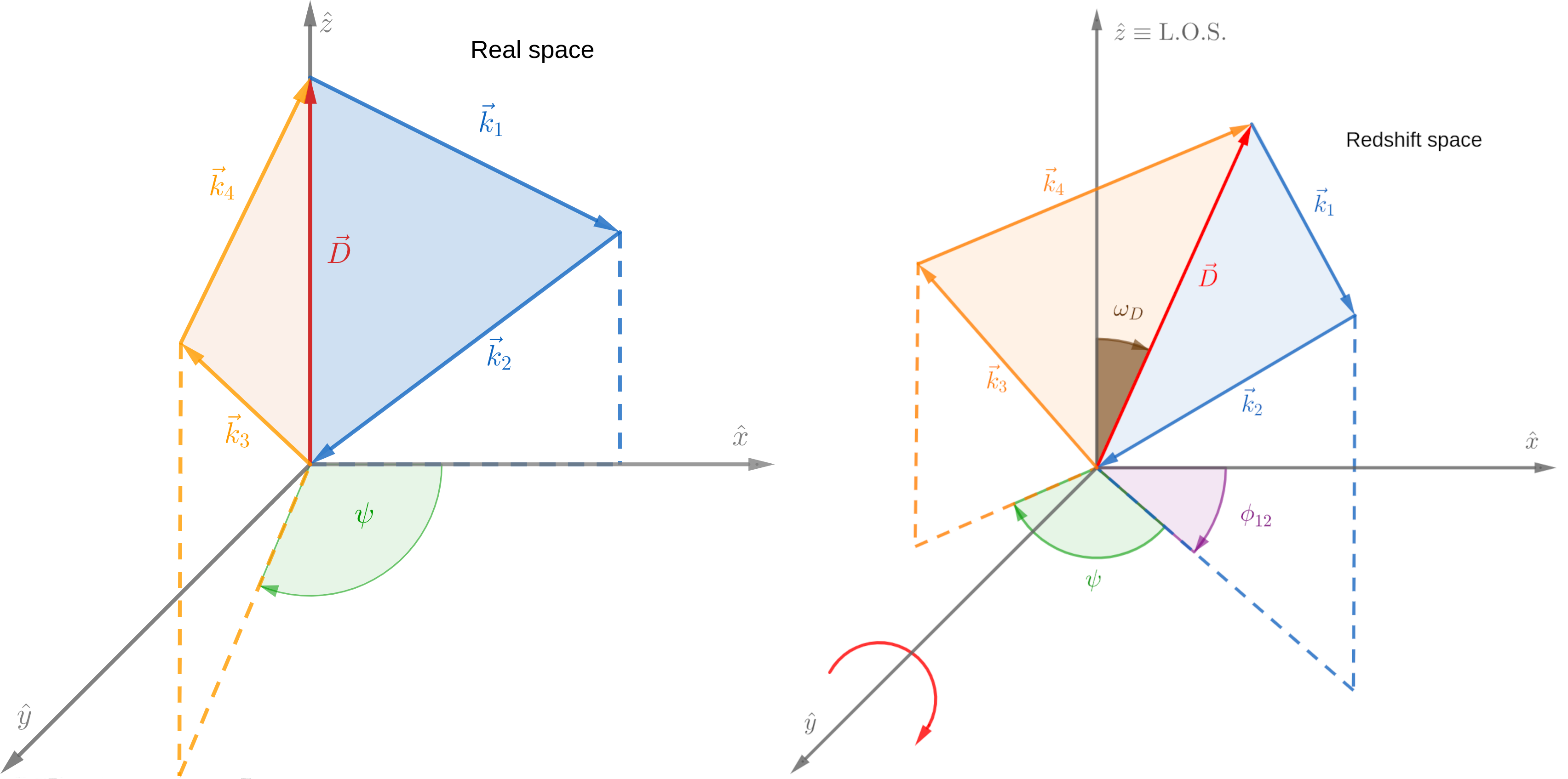
The matter trispectrum (in real space) is a statistic measured on an isotropic field. This reduces the number of degrees of freedom necessary to describe a quadrilateral configuration from eight (needed when the signal depends on the orientation with respect to the line of sight) down to six.
Here we use the convention illustrated in figure 1. We use as diagonal, , the one defined by . The module of this diagonal can then vary between a minimum and a maximum value defined by
| (2.5) |
where the above conditions are imposed by the requirement that the triangles formed by the diagonal and the two -vectors (, and , ) are closed. In real space, the orientation with respect to the line of sight does not matter and therefore, for each quadrilateral, one could choose to set the diagonal vector parallel to the line of sight direction (namely, -axis). With this choice, the two triangles defined by and will be orthogonal to the -plane.
Finally, the angle describes the "folding" of the quadrilateral around the diagonal , in other words, the angle between the two planes defined by the two triangles and . It should be then clear that where are varying only in the redshift space case (see section 2.1.1), because each set corresponds univocally to a set and vice versa. We choose to study an averaged version of the trispectrum signal which we call i-trispectrum, with each configuration described only by the modulus of the four quadrilateral sides, . In other words, we integrate out, by averaging over all their possible values, the additional two coordinates needed to fully describe a quadrilateral configuration (in real space). According to our adopted convention (figure 1) this means integrating over and . The redshift space i-trispectrum (see section 2.1.1) monopole is further averaged over and .
Therefore, differently from what happens for the power spectrum (line) and the bispectrum (triangle), the i-trispectrum signal as a function of just is an average over many different shapes characterised by different values of one diagonal and the folding angle around it . The second diagonal that could be used as coordinate and its folding angle is fixed by choosing the first coordinates pair .
Following these conventions, we define matter i-trispectrum in real space as a function of the module of the four -vectors as
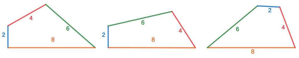
where . Given a set, three different shapes can be obtained by changing the order of the sides, this being the reason for the average in equation 2.1.
This can be understood by looking at the sketch in figure 2. The three different shapes are obtained by changing the ordering of the sides ; for simplicity quadrilaterals shown lie on a plane i.e., no folding around the diagonal is shown in the sketch, where the diagonal is always defined from the first two entries of ’s arguments.
From equation 2.1 is easy to appreciate the improvement over [83] comparing with their equation 34. While they approximate the theoretical model for the integrated trispectrum estimator using an amplitude factor, here we perform explicitly the full multi-dimensional integration in Fourier space.
The corresponding estimator applied on data will be later defined in equation 2.16. In appendix A the theoretical models for redshift space power spectrum, bispectrum and trispectrum are briefly reported.
2.1.1 Redshift space i-trispectrum: coordinates
When redshift space distortions are present, and in the partial sky/plane parallel approximation, the signal is not isotropic anymore [48, 41]. The preferred direction is given by the line of sight, which, by convention, we align with the direction. Hence, compared to the real space case discussed above, in order to define the orientation with respect to the line of sight of all the possible quadrilaterals (defined by the set of coordinates ), only two additional parameters are necessary.
First we define an angle to describe the rotation of the triangle away from the -plane (illustrated in the right part of figure 1).
As remaining parameter we choose the cosine of the angle between the diagonal, , and the line of sight, . Then by rotating each vector by an angle , together with the choice of angles , all the possible orientations/shapes can be defined (and spanned when integrating over).
It is indeed important to notice that the orientation with respect to the quadrilateral line of sight, together with its shape, can also be modified by varying both angles and . These three variables may be used as a natural basis for an expansion in terms of Legendre polynomials of the full anisotropic i-trispectrum signal. The redshift space i-trispectrum monopole can be obtained by performing the four-dimensional integration of the redshift space trispectrum, :
| (2.7) | |||||
2.2 Estimators: measuring P, B, of an overdensity field
Given an overdensity field, we need a procedure to estimate the statistics of interest: power spectrum, bispectrum and i-trispectrum. The overdensity field, as sampled for example by particles or haloes in an N-body simulation or by galaxies in a survey, is a discrete distribution, which contains a shot-noise contribution to the measured statistics. The first step is then to distribute through a mass assignment scheme (see for example [45, 82]) each particle’s contribution to a cell in a three-dimensional discrete grid, in order to derived a pixelised overdensity distribution . Then, estimators should be adapted to take advantage of discrete Fast Fourier Transforms algorithms (FFT) [29]. This procedure is described in detail in appendices B (and C for what concerns the shot-noise subtraction). We review here the key steps and present the main results derived following the approach introduced by Refs. [74, 75] and used also in Ref. [97]. We will start here writing integrals (as in an idealized case where the fields were continuous and the volume infinite) and not discrete sums (realistic case for pixelized fields and finite volumes) to define the estimators in Fourier space to better show the fundamental connection between theoretical modelling and numerical implementation of the estimators. Given a cubic realisation of size and volume , the overdensity is usually pixelised within cells whose volume is .
Starting from the expressions for the direct and inverse Fourier transforms of the matter density perturbation field,
| (2.8) |
where the integration is over the whole volume in configuration and Fourier space, the following quantities can be defined:
| (2.9) |
where the integration is over the spherical shell with radius defined by the -vector module and with thickness . Given these ingredients, we can define the integral version of the power spectrum estimator (bandpower evaluated in a thin shell around ):
| (2.10) | |||||
where is the Dirac’s delta and where each integral is performed over a spherical shell of radius for and thickness , the width of the bandpower. is the number of pairs found inside the integration volume in Fourier space, where is the integration volume in Fourier space while is the box’s fundamental frequency. Converting the integrals into discrete sums as described in appendix B the estimator becomes
| (2.11) |
where and (full expression reported in equation B.1) denote the pixelized ( stands for discrete as a pixelized version of a continuous field is often referred to as “discretized") of the quantities defined in equation 2.9 for a grid with cells.
Similarly, for the bispectrum we start from the unbiased estimator
| (2.12) | |||||
where is the number of triangles included in the integration volume in Fourier space ( is the integration volume in Fourier space for the bispectrum). As for the power spectrum, the above estimator can be expressed in terms of discrete sums (see equation B.2):
| (2.13) |
2.2.1 i-trispectrum
The idea to define an estimator for the trispectrum which depends only on the magnitude of the four -modes defining the quadrilateral was pioneered by [83]. Here, using the approach of [75] we make the estimator fast enough to be applicable to a large set of independent synthetic realisations and eventually on data and, by performing explicitly the angular integrations, make it transparently connected to the theoretical model for the trispectrum.
Analogously to the power spectrum and bispectrum, the estimator for the four-point correlator could be defined as a quantity proportional to a suitable average of four modes. However, differently from the power spectrum and bispectrum cases, this will not be a particularly useful i-trispectrum estimator; when taking the ensemble average of such quantity, two terms appear –according to Wick’s theorem–: a connected (c) and an unconnected (u) part.
So the estimator simply identified with the four-point correlator estimator will include both these contributions:
where is the number of skew-quadrilaterals in the integration volume in Fourier space (see [39]’s appendix for a derivation of the trispectrum integration volume in Fourier space ). Notice that this estimator automatically averages over all the possible shapes and permutations included in the model of equation 2.1.
In fact,
| (2.15) |
where denotes the connected i-trispectrum part, and the three permutations of the product of two terms proportional to the power spectrum () are the unconnected part. The unconnected part is not of particular interest here, since it is completely determined by the field’s power spectrum.
The signal of interest and the one we want to isolate is the connected part, the i-trispectrum. In other words, the i-trispectrum estimator should be obtained by subtracting the unconnected part from the total signal measured by the four-point correlator estimator in equation 2.2.1:
| (2.16) |
In the cosmological context of interest and for Gaussian initial conditions, perturbation theory predicts the unconnected part (which is intrinsically a linear order quantity) to be dominant with respect to the connected one (which is intrinsically third order). This will later be proven using the simulations measurements, with the unconnected part resulting to be two orders of magnitude larger than the connected one.
As derived in appendix B.3.1 the discretised estimator for the total signal of the four-point correlator in Fourier space is888Recall that we describe the i-trispectrum using only the four sides of the quadrilateral as coordinates and not also the diagonal (as introduced to compute the theoretical expression for the estimator). This is motivated by numerical computation time considerations. If we had used the diagonal as additional coordinate, by writing the estimator with the closure conditions , in the above expression there would have been a double sum over each grid element, implying a computation scaling as instead of . Introducing the diagonal here is not necessary because the estimator defined as a function of automatically integrates over all possible shapes given by the allowed values of the diagonal (and the folding angle ).
| (2.17) |
In order to isolate the unconnected term and to subtract it from the total signal measured from the simulations we define the estimator
| (2.18) |
where the above expression captures the fact that the unconnected part by definition is non-zero when at least one of the terms – each involving product of the two-point correlators – is non-zero. This contribution then appears only for those quadrilaterals sets with two pairs of equal sides (or all four equal sides). The corresponding discretised estimator is (appendix B.3.2)
| (2.19) |
From equation 2.2.1 we can also derive an analytical expression to model the unconnected signal of the four-point correlator in Fourier space (see equation B.3.2 for the derivation):
| (2.20) |
where denotes the Kronecker delta for and is a symmetry factor whose value is one in case the quadrilateral has two pairs of equal sides, three if the four sides are the same and zero otherwise. It is important to notice that since the quadrilateral diagonal is not a fixed parameter given the four sides, . are the bin sizes chosen for the -modes and the diagonal . These will be later defined in section 3.1.1 in terms of the fundamental frequency given by the analysis set-up.
We are aware that another option would be to simply discard all the symmetric configurations and by doing so avoiding the quadrilaterals sets whose i-trispectrum has an unconnected part. While an interesting avenue to explore, we find that it would imply a loss of constraining power, therefore here we proceed with the estimator of equation 2.16, since it allows harvesting the information contained in the i-trispectrum of symmetric configurations.
2.3 Covariance matrix estimation and modelling
The power spectrum, bispectrum and i-trispectrum for different -bins, triangles and quadrilaterals sets can be organised into a data-vector. In our case, the measured power spectrum, bispectrum and i-trispectrum joint data-vector is given by the elements
| (2.21) |
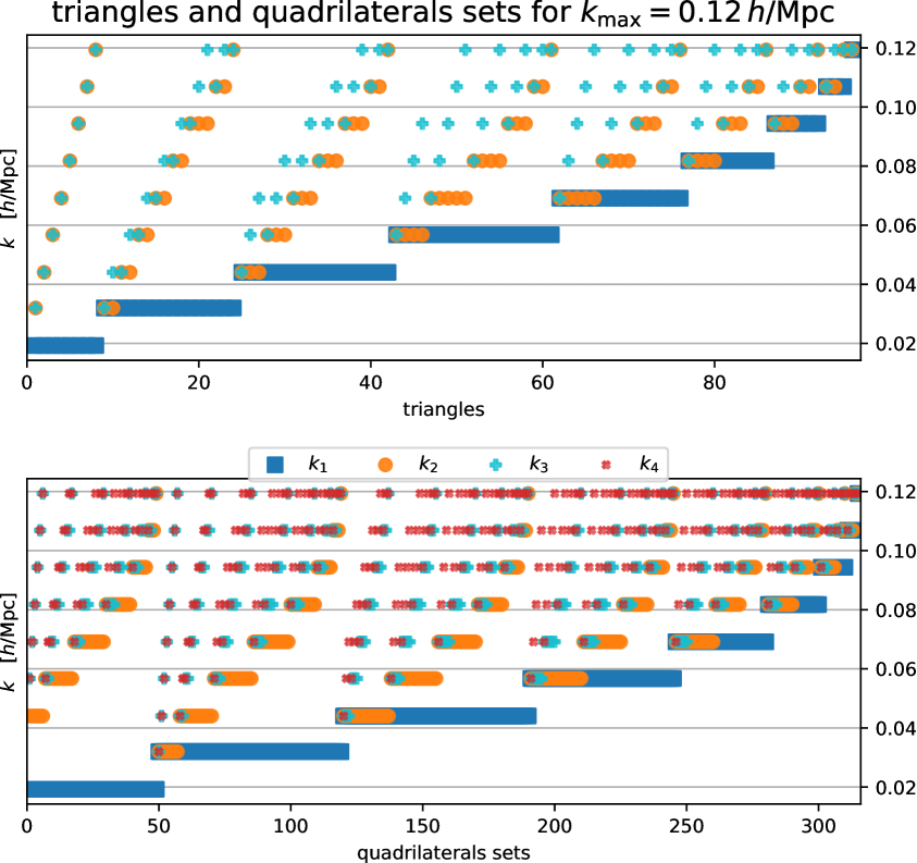
where each statistic is characterised by its own maximum -value, . The theoretical counterpart of this data-vector is composed by the adopted model for each of the statistics, which we label . Sometimes for brevity we will refer to as the data-vector defined above measured for the same for all statistics. The configurations ordering for both bispectrum and i-trispectrum in terms of the -values of the triangle and quadrilaterals sets sides is shown in figure 3. In order to avoid double-counting shapes, once is chosen the other sides respect the ordering and for triangles and quadrilaterals sets respectively. In the figure, (in blue) increases from left to right and the -axis reports the label (index) of the configuration. For each configuration the figure shows the length of (orange), (cyan) and (red).
Besides the estimator for the statistic of choice (which comprises the elements of the data-vector ) and the theoretical expression of the estimator (elements of ), the remaining key ingredient of all the parameter constraints analyses and forecasts is the covariance matrix, which encodes the uncertainty and correlation present in the data-vector. The uncertainty is related to the error associated with the individual element measurement while correlation quantifies how dependent to each other the different elements of the data-vector are.
The covariance matrix of the i-trispectrum and the cross-covariance with power spectrum and bispectrum are fundamental ingredients for assessing the impact of adding this four-point statistic to a parameter constraints analysis. In what follows, for brevity we refer to the full joint power spectrum, bispectrum and i-trispectrum covariance, or data-vector, as PB. Usually in this kind of forecasts studies, an analytical template is used and often the covariance is assumed to be diagonal (i.e., no correlation between different -bins), with only a Gaussian component (i.e., ignoring contributions from non-linear clustering), together with assuming no cross-correlation between different -point statistics.
Alternatively, given a set of measurements from independent realisations of the data-vector of interest, the covariance matrix can be numerically estimated by
| (2.22) |
where is the number of independent realisations (here we use 5000 realisations see section 3.1) used to measure the data-vector and denotes the average across the whole set of realisations and denotes the transpose.
The inverse of a covariance matrix estimated from a finite number of realisation is known to be biased [42, 84]. We correct this by using the Hartlap factor [42], where is the data-vector’s size while is the number of simulations used to estimate the covariance (5000 in our case999While the Quijote [101] suite offers more than 5000 realisations, we only use 5000 for each redshift for computational reasons. Given the maximum length of our data-vector, this number is more than enough to estimate the inverse of the covariance matrix. In fact the Hartlap factor is or higher.). Notice that when . A more accurate correction to the inverse of the covariance matrix estimated from a finite number of independent realisations and its effect on the resulting likelihood was introduced by [84]. We tested that for the purpose of evaluating the added benefit of including the i-trispectrum in the analysis, the difference between the two corrections is negligible.
Often the lack of a large number of independent realisations is the reason why resorting to an analytical model for the covariance is appealing. In particular, if the overdensity field can be approximated by a Gaussian random field, the covariance matrix can be modelled analytically (especially for simulated cubic boxes). We refer to this approximation as Gaussian and its non-zero terms in the covariance as Gaussian terms. Recent studies on the power spectrum and bispectrum covariance matrices and their analytical models can be found in Refs. [89, 102, 39].
For what concerns the i-trispectrum, we compute, for the first time, the Gaussian terms at leading order following the approach developed, for the power spectrum and bispectrum, in [38, 37].
The real space matter field i-trispectrum covariance matrix is a specific case of the more general covariance in redshift space for biased tracers, whose derivation is reported in the appendix D at equation D.1. Since the kernels of the real space matter field do not depend on the relative orientation of the -vectors, and there is no dependence of each -vector orientation with respect to the line of sight, no integration is required. Consequently, the analytical expression for the diagonal elements of in the Gaussian approximation (see equation D.1 for full expression) reduces to
| (2.23) |
where the expression of the Fourier integration volume, , is given in equation B.3.2; is a symmetry factor (given by , where is the number of repeated modules) that counts the number of possible permutations of equal sides between the two identical quadrilaterals sets, and its values for a given symmetry are given in equation D.2; is the effective survey volume.
We will compare the diagonal elements of the covariance numerically estimated from the simulations with the above theoretical model later in section 3.1.4 to show that for the i-trispectrum the Gaussian approximation is only reasonable at high redshifts.
2.4 Primordial non-Gaussianity imprint on the i-trispectrum
Deviations from Gaussianity of the primordial gravitational potential [8] are a powerful tool to constrain models of inflation [10] describing how the large-scale structure we currently observe was generated. In this work we focus on primordial non-Gaussianities (PNG) of the local type which are parametrised by an amplitude parameter (we will refer to it as from now on for simplicity). The Bardeen’s gravitational potential [8] can be written as a polynomial expansion in terms of a Gaussian field with coefficients and up to third order:
| (2.24) |
where is the speed of light which is needed in the expansion since in this formalism has units of . For more details see appendix E.
A detection of would rule out single field inflationary models since they predict a much smaller value of the same parameter [61, 19], while at the same time it would favour multi-field inflationary models or alternatives to inflation. At the moment of writing, the tightest constraints, from the Planck analysis of CMB data, are (at confidence level) [4]. For large-scale structure, using the DR14 eBOSS quasars sample and exploiting the scale dependent bias effect induced by primordial non-Gaussianity [21, 62] (see [9] for a recent study on the impact of galaxy bias uncertainties on PNG constraints), the state of the art constraints are (at confidence level) [15].
To date, only the bispectrum has been thoroughly studied in the literature for its sensitivity to primordial non-Gaussianity signatures at the lowest-order in perturbation theory [100, 53, 79, 46, 78]. Recently Ref. [39] suggested that the bispectrum anisotropic signal could boost even further the late-time constraints on . The expressions for the primordial non-Gaussianity contributions to the matter power spectrum and bispectrum are reported in appendix E.
The large-scale structure trispectrum as a test for Gaussianity of the initial conditions was proposed in [98]. Since then the trispectrum has been mainly considered for CMB analyses, targeted to produce constraints on primordial non-Gaussianity [66, 64, 50, 72, 43, 85, 25], in particular with Planck [24] deriving constraints on both and . For what concerns late-time analyses, the 21-cm background anisotropies trispectrum was studied in Ref. [18], while Ref. [11] included the trispectrum of LSS to measure the energy-scale of inflation through its relation with primordial non-Gaussianities.
As described in detail in appendix E.3, and following [46, 79], one can see that in the presence of primordial non-Gaussianity, when expanding the four-point correlator (with shorthand notation ) whose connected component is the trispectrum, four terms appear:
| (2.25) |
The third and fourth terms, and , represent the standard trispectrum due to gravitational collapse (when limiting the expansion to order , or in terms of the Gaussian primordial potential ). The first term produces two terms proportional to and , respectively. The second term is a mixture of primordial non-Gaussianity and gravitational non-linear evolution and it is proportional to . Therefore the model for the primordial non-Gaussianity imprint on the matter trispectrum in real space, , is given by101010The corresponding redshift space quantity for the matter field is simply obtained by replacing the matter case kernels with the redshift space ones as done in appendix A for the purely gravitational terms and .,
where , with being the linear growth factor, the matter density parameter, the Hubble constant and the transfer function. From the above equation we can see that the term that has the potential to significantly improve the bispectrum constraining power for is . This is because has a similar functional form and -dependence as the matter bispectrum PNG correction (equation E.29 in the appendix).
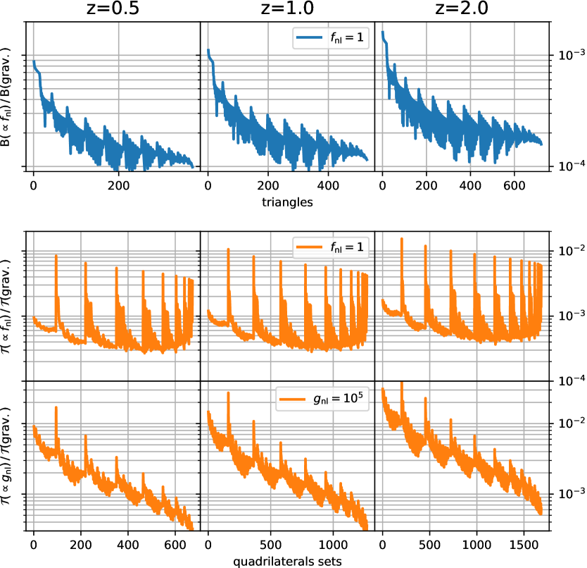
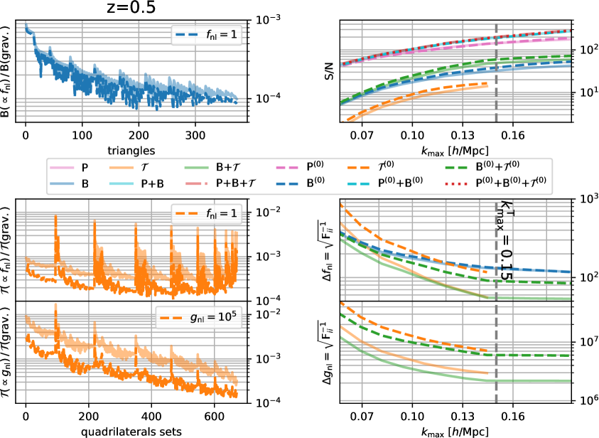
Figure 4 shows, for matter bispectrum and i-trispectrum in real space, the ratio between primordial and gravitational components for and . For the bispectrum, as expected, the ratio is depending on scale, for the i-trispectrum there are configurations where this ratio is larger and reaches . These are symmetric configurations of the i-trispectrum and the boost is driven by the sum of -vectors appearing at the denominator of one of the two components of reported in equation 2.4.
2.5 Fisher-based forecasts
Before developing all the required theoretical and technical tools necessary to employ a new statistics in the analysis of real survey data, there are mainly two ways to assess the additional information harvested by measuring this new statistics on a cosmological field. One method is to look at the general improvement of the full data-vector signal-to-noise (including both old and new statistics). The other, more specific, alternative is to forecast the improvements on the parameters of interest constraints obtained by employing the new statistics.
With the covariance matrix for a given data-vector in hand, we can define two quantities for these purposes. These are the cumulative signal-to-noise (S/N) and the Fisher information matrix (F); from the latter, both conditional and marginalised errors on the model parameters can be estimated.
The (expected) cumulative signal-to-noise as a function of the maximum -value, given a (theoretical description of a) data-vector and the relative covariance matrix , is computed as
| (2.27) |
where the data-vectors should be interpreted as functions of .
Given a theoretical model description of the data-vector, , with dependence on model parameters , the Fisher information matrix is the Hessian matrix of the associated log likelihood, , with the derivatives taken with respect to the model parameters,
| (2.28) |
where indicates that the derivatives are evaluated at the likelihood maximum.
In the case of a single-parameter estimate, the minimum achievable error is given by . In the general multi-parameter case, this is the conditional error as it assumes that all other parameters are perfectly known. To obtain the marginal error, in the multi-parameter case the inverse of the Fisher information matrix needs to be used [94]. Using the data-vector’s covariance matrix and its derivatives with respect to the model parameters, each element of the Fisher information matrix can be computed as
| (2.29) |
since here (as in most Fisher forecasts and in most large-scale structure studies) we adopt a Gaussian likelihood with fixed covariance matrix (see e.g., [14, 49]).
In what follows we will make use of another related quantity: the cumulative as a function of . Given a measured data-vector and its theoretical model , the cumulative can be computed using the full covariance matrix, , or can be approximated (as often done in practice) by considering only the diagonal elements, . These expressions read,
is a shorthand for the data-vector with configurations limited by (same for the covariance ), while and are the mean and the variance for the -th mode (with running over all the elements of the data-vector ) estimated from the set of simulations. Here we assume (as often done) that the number of degrees of freedom, , corresponds to the length of the data-vector up to a certain minus one. includes the cross correlations among different elements of the data vector, , on the other hand, assumes the different data-vector elements to be uncorrelated and therefore uses only the variance. The is popular because it offers a relatively quick, although often inaccurate, goodness of fit test.
Notice that while in our analysis we will adopt the mean of the measured data-vector as reference for the -test, we will not use the error on the mean (which would be computed by dividing the variance in equation 2.5 by the number of realisations used), but the one relative to a single realisation. This is because deriving a dark matter statistics model which would be accurate enough to return a good for an average over thousands of is beyond the scope of this work.
3 Results
3.1 Real space: measure vs. model
In this section we compare the measurements of the power spectrum, bispectrum and i-trispectrum estimators from the set of Quijote simulations [101] to the respective theoretical models (section 2.1) for three different redshift snapshots: , , . We also measure the i-trispectrum auto and cross (with power spectrum and bispectrum) covariance matrix, and compare its diagonal elements with an analytical model.
3.1.1 Analysis set-up
We use 5000 realisations of the N-body simulations from the Quijote suite [101]. Given the lenght of our data vector we estimate that offer an optimum balance between speed and computational resources and accuracy of the estimate of the covariance matrix and its inverse. The simulations follow the gravitational evolution of dark matter particles, in a periodic cubic box with size . The initial conditions for the simulations were generated at using 2LPT [87, 20, 77], and we concentrate on the snapshots at redshifts , and .
The underlying cosmology of the Quijote simulations is a flat CDM model (consistent with the latest CMB constraints [17]). Specifically, the matter and baryon density parameters are , , and the dark energy equation of state parameter is ; the reduced Hubble parameter is , the late-time dark matter fluctuations amplitude parameter is , the scalar spectral index is , and neutrinos are massless, i.e. eV.
We discretise the box in grid cells, and consider a bin size of , where is the fundamental frequency. Since non-linearities increase as the redshift decreases, perturbation theory, and hence our model, breaks down at different scales for different redshifts. In the following analysis the quadrilaterals sets sides for the i-trispectrum are limited to , and . For both power spectrum and bispectrum we display results for a which is one third larger than the one for the i-trispectrum at each redshift (i.e. , and ). In what follows, the triangles (for the bispectrum) and quadrilaterals sets (for the i-trispectrum) are ordered and labelled according to the convention illustrated in figure 3.
We assume a Poissonian shot-noise and we subtract it from the measured signal using the procedure described in appendix C. This consists in using measured quantities (such as power spectra and bispectra) to build the shot-noise corrections given in the literature e.g., [98].
3.1.2 Power spectrum and bispectrum
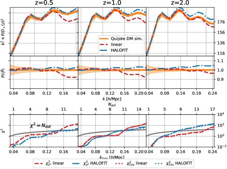
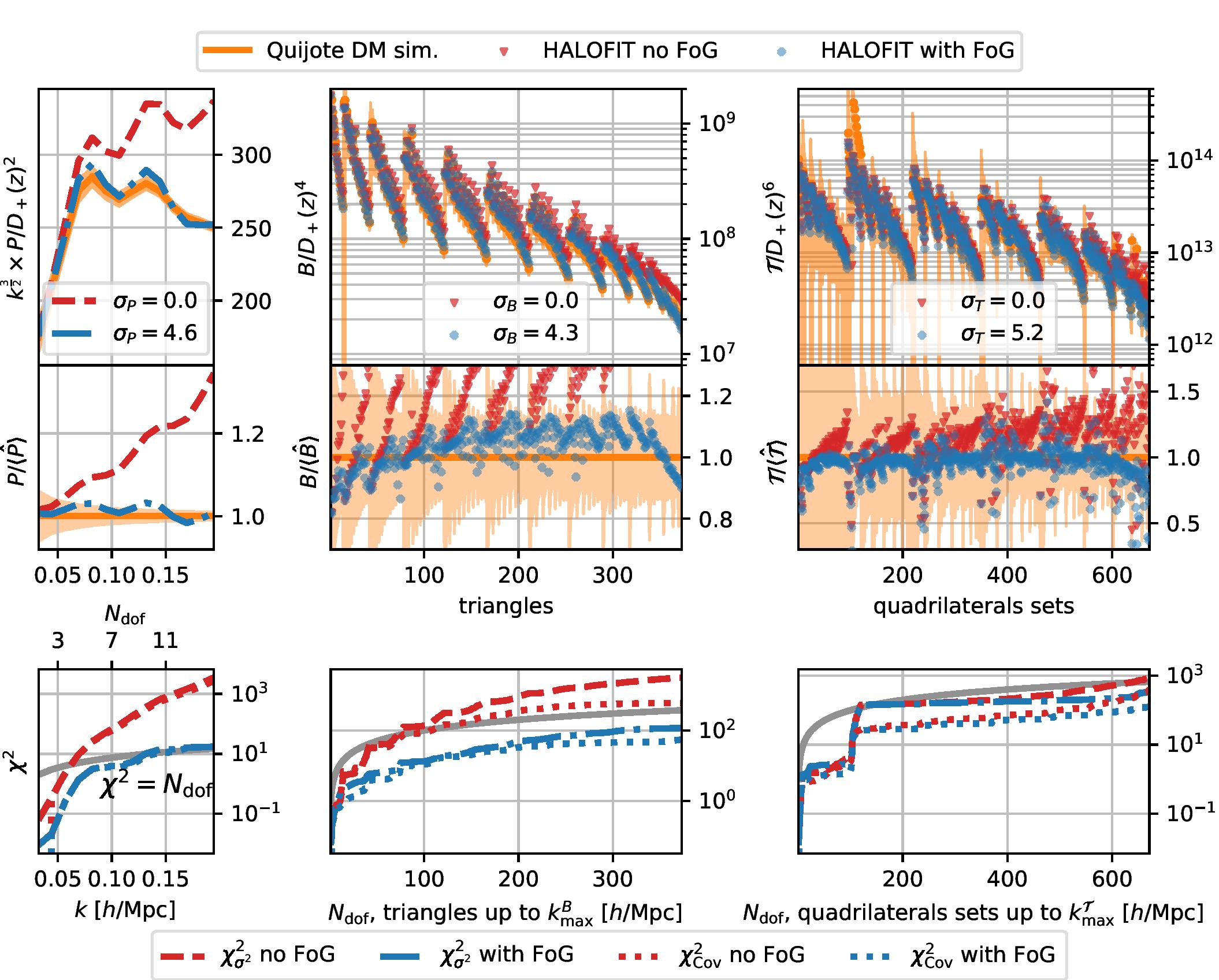
In figure 5 the mean and the standard deviation of the power spectrum measurements from the Quijote simulations (orange solid lines) are compared to the theoretical model predictions. The adopted -bin size is and the rms is computed by the scatter among the 5000 realisations. Both linear theory (red dashed) and halofit (blue dot-dashed) predictions are shown. In the first row the power spectra are multiplied by a factor of and normalised by the linear growth factor squared at each snapshot’s redshift, , also computed using class. The next row shows the ratio between the theoretical models and the simulation measurement (simulation output in orange, halofit in blue dot-dashed and linear theory prediction in red dashed). The third row shows the cumulative computed as described in equation 2.5. It is possible to appreciate the redshift dependence of the up to which the models fit the data well. While for and halofit performs better than the linear power spectrum prediction, at the opposite happens and the linear model has a good up to . This effect is understood as follows. In this range of scales at this redshift many -modes are undergoing gravitational collapse simultaneously (for those values such that , which is the regime where structure formation is more complex to describe with halo-model/semi-analytic approaches. On the other hand, at later times, when the structure formation may be more nonlinear (and naively more difficult to model), the collapse happens in a more ordered way, and it is easier for Halofit to capture it. One should also recall that Halofit is designed to match the power spectrum shape up to , so it is not surprising that its description of the power spectrum is not too accurate at relatively weakly non-linear scales.
The cumulative chi-square computed with and from equation 2.5 almost perfectly overlap: at these scales the power spectrum modes are not very correlated and the covariance matrix is quasi-diagonal.
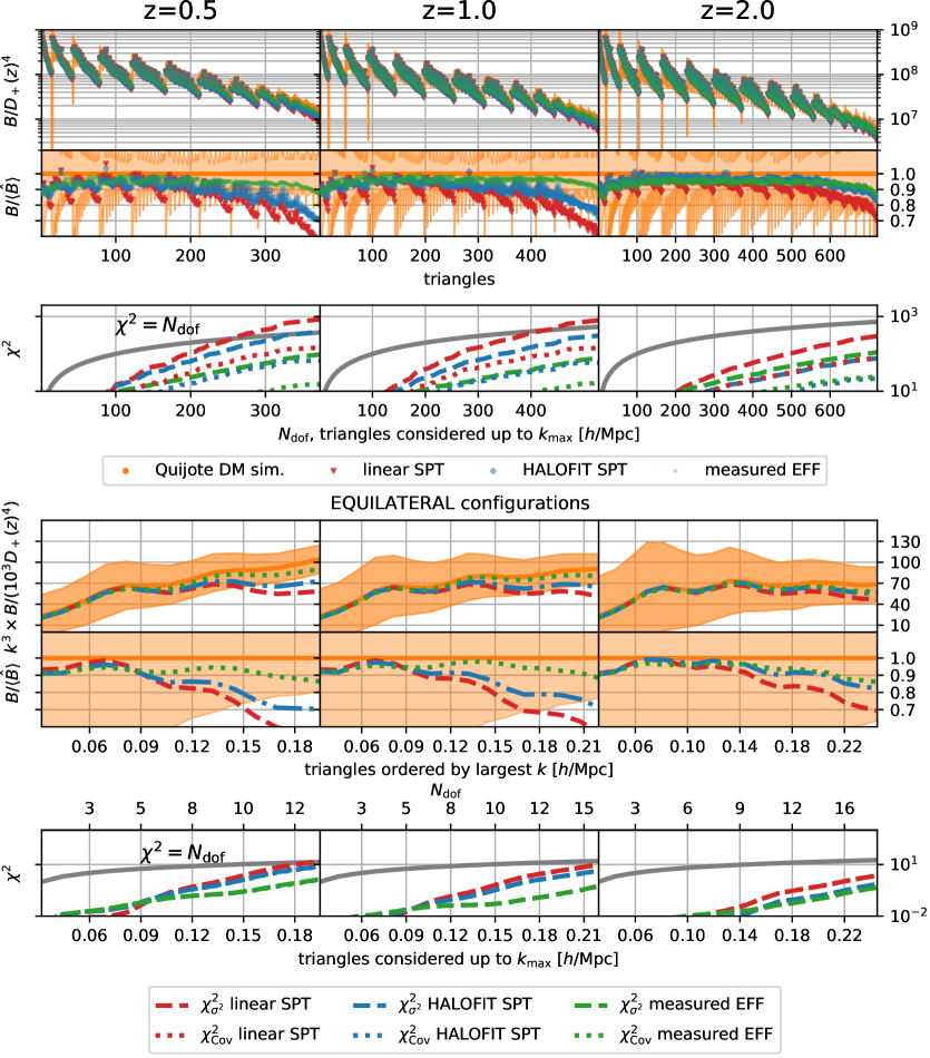
Figure 6 shows the same information for the bispectrum. In the top half of the plot all triangle configurations are shown, while the lower half displays only equilateral configurations in order to make the scale dependence easier to interpret.
In addition to the SPT models using the linear and halofit power spectra as input ( and ), we also present the comparison of the measurements with the effective model (see equation 2.2 and Refs. [31, 34]). In this case we use the mean of the power spectrum measurements from the simulations as non-linear power spectrum input for the effective model ("measured EFF" in the figure). The SPT model with halofit non-linear power spectrum always outperforms the standard SPT one (with linear power spectrum) and becomes closer to the effective bispectrum model as the redshift increases. At all redshifts, the effective bispectrum model significantly increases the maximum at which the model fits the measurements. It is interesting to note how the model, with the effective kernel calibrated for only specific shapes from N-body simulations, offers a better description than SPT for all triangle shapes.
The difference between the cumulative assuming uncorrelated bispectrum modes and accounting for the full covariance, and (equation 2.5), is visible in the “all shapes" case (top half of the plot): different bispectrum modes (triangles) are in general correlated; equilateral configurations on the other hand are only very weakly correlated.
3.1.3 i-trispectrum
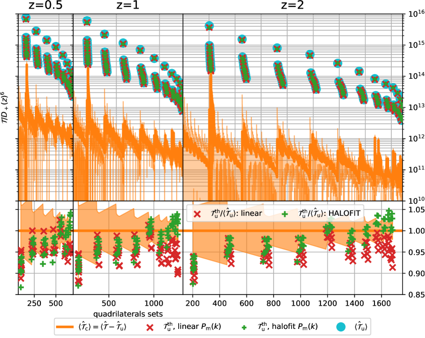
As described in section 2.2.1, in order to obtain the i-trispectrum signal, the unconnected part needs to be subtracted from the total signal measured using the estimator presented in equation 2.2.1. In figure 7 we compare the unconnected signal theory template , (equation 2.20) with the measurement performed using the estimator in equation 2.2.1. The unconnected part is approximately two orders of magnitude larger than the connected part (which is expected from standard perturbation theory, being the unconnected part a lower order term with respect than the connected one).
To avoid systematic errors due to limitations in the perturbation theory description of the unconnected part of the signal, we prefer to estimate the unconnected contribution using equation 2.2.1 instead of the analytical model. This is to be subtracted from the total signal to obtain the i-trispectrum according to equation 2.16. In the lower panel of figure 7 the ratio between the models for the i-trispectrum unconnected part using linear and halofit matter power spectra can be seen to diverge from one as the size of the quadrilateral sides increases, as expected from the breaking down of perturbation theory at non-linear scales (see figure 3 to visualise how the sides vary among configurations).
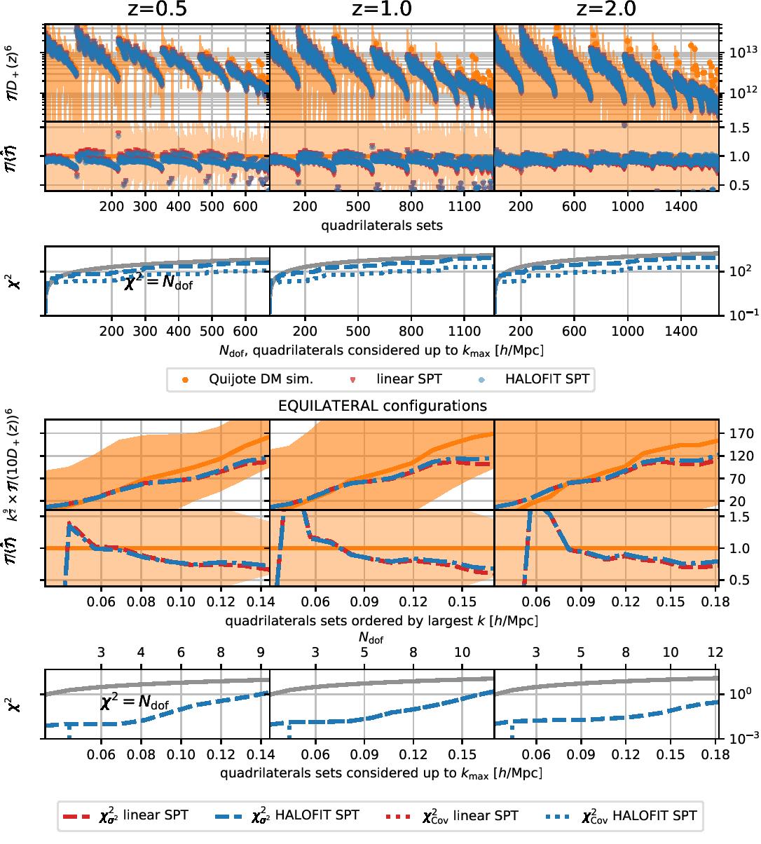
In figure 8 we show the comparison between the resulting measured i-trispectrum , and the theoretical model, defined in equations 2.4 and 2.1 (same conventions as for figure 6). For easier interpretation, in the lower part only equilateral configurations are shown.
The integrated theoretical model (equations 2.4 and 2.1), both for linear and halofit power spectrum, performs reasonably well. When all the quadrilaterals sets are considered, the cumulative closely follows the line for our adopted , number of degrees of freedom. Notice that the different quadrilaterals sets making up the i-trispectrum data-vector are correlated, as it can be inferred from the covariance matrix shown in figure 9, therefore the effective number of degrees of freedom is effectively lower than the number of configurations used.
An improvement in the fit could be obtained by extending the effective model of the kernels to the third-order ones needed to compute the i-trispectrum. At the same time the second order kernels could be fitted using both bispectrum and i-trispectrum. We leave this to future work.
3.1.4 Covariance matrix and Gaussian term analytical model
The covariance matrix of the i-trispectrum and that of the full power spectrum, bispectrum and i-trispectrum data vector (PB for short), are fundamental ingredients for assessing the impact of adding this four-point statistic to a parameter constraints analysis. Usually in this kind of forecasts studies, an analytical template is used and often the covariance is assumed to be diagonal with only a Gaussian component, together with assuming zero cross-correlation between different -point statistics.
In this section we show that following the above assumption in the case of the i-trispectrum would induce a significant bias leading to an overestimate of the i-trispectrum constraining power when added to the power spectrum and bispectrum data-vector. To this purpose, we numerically estimate the PB covariance matrix from the simulations as described in section 2.3. The at each redshift for each statistics are the same as described in section 3.1.1.
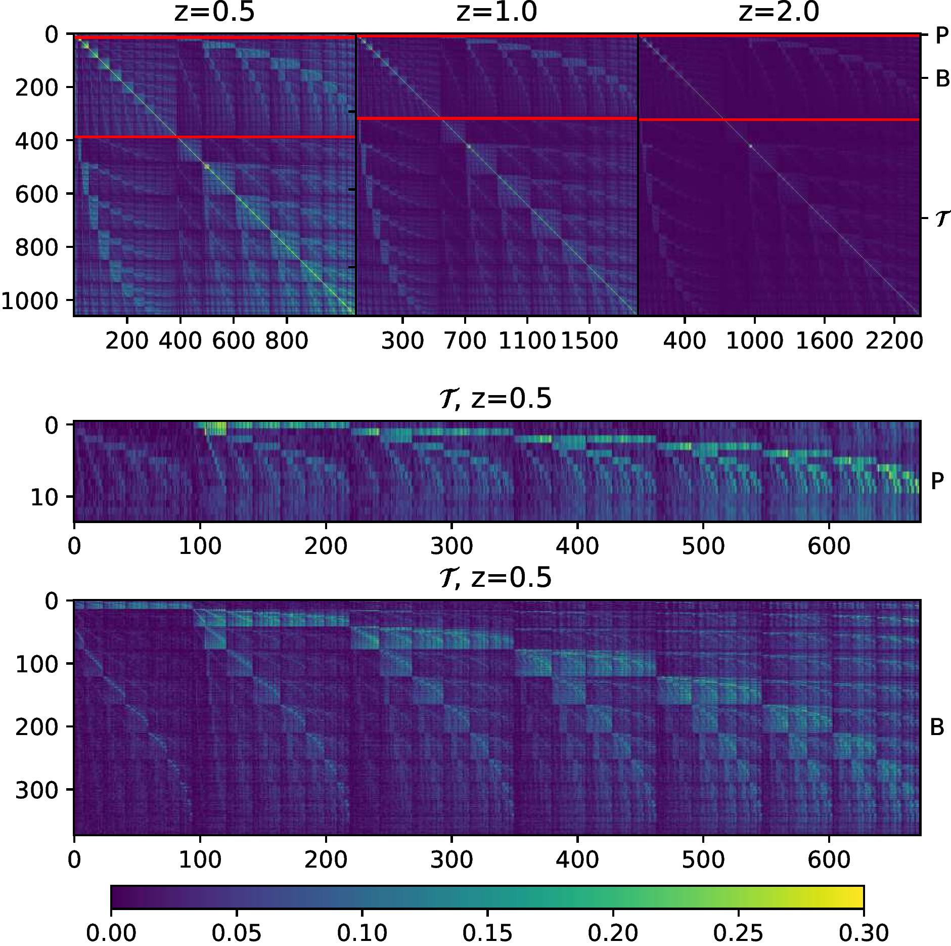
Figure 9 shows the reduced covariance matrix, , numerically evaluated from the 5000 simulations. The top row shows the full (PB) covariance (to guide the eye, the red lines indicate the P, B and sections). In the central and bottom rows of figure 9 the cross-correlations of the i-trispectrum with both power spectrum and bispectrum are displayed at . As the redshift increases it is evident how the different elements of the joint data-vector become less and less correlated since the field is more linear and the mode-mixing induced by gravitational collapse is less important. At redshift for the i-trispectrum, the off-diagonal elements of the reduced covariance become up to . This means that two different configurations can be cross-correlated as much as one third of their auto-correlation value. In other words, the level of redundancy in the data-vector increases as the redshift decreases.
Note also that the cross-correlations between power spectra of -modes and bispectra of triangle configurations with the i-trispectra of quadrilaterals sets (up to the i-trispectrum ) are non-negligible at low redshifts.
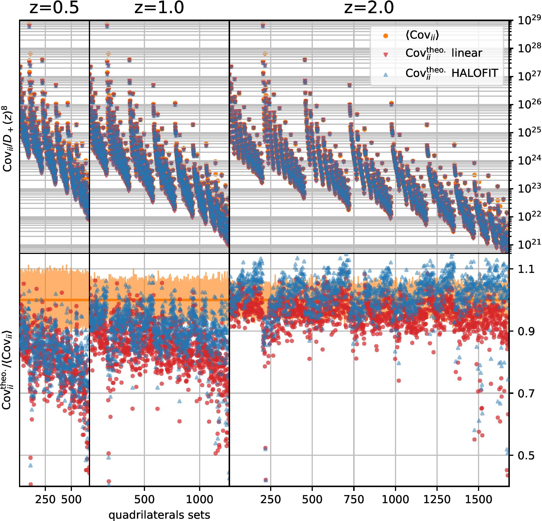
A quantitative idea of the importance of the non-Gaussian contributions appearing in the i-trispectrum covariance matrix can be obtained by comparing the analytical model of the diagonal Gaussian term of equation 2.23 with the one estimated numerically. This is shown in figure 10: the difference increases as the redshift decreases. The shaded area is obtained by estimating the scatter of the covariance diagonal elements as follows. We take measurements from groups of simulations boxes randomly selected from the whole set of 5000 realisations. The is set by requiring that the number of simulation boxes per group (i.e. ) is no smaller than half of the data-vector dimension. Note that the number of realisations used to estimate the covariance can safely be lower than the respective data-vector’s dimension since we are just interested in deriving the diagonal elements, without inverting the covariance [42]. This confirms what is seen in figure 9, that for the i-trispectrum data-vector the non-Gaussian terms in the covariance are not negligible, in particular at lower redshifts.
The visible difference between and (equation 2.5) in figure 8 when all the configurations are considered further supports the importance of going beyond the Gaussian diagonal covariance approximation for the i-trispectrum (and also previously in figure 6 for the bispectrum) also for evaluating the goodness of fit of a theoretical model.
3.2 Primordial non-Gaussianity constraints: forecasts
For local primordial non-Gaussianity, a first assessment of the additional constraining power given by the i-trispectrum can be made via a Fisher-based forecast, considering the real space matter field. Promising results in this idealised case can motivate a more realistic analysis (e.g., for biased discrete tracers, in redshift space).
Moreover, in this conservative scenario, we only consider conditional errors on the non-Gaussianity parameters, i.e., assuming all other parameters are fixed. If these were let free to vary, we expect the improvements on the constraints given by the i-trispectrum to be larger due to the reduction of the degeneracies present in the parameters space. This expectation is motivated by the analogy with the findings of [81, 16, 103, 40, 3] obtained when adding the bispectrum to the power spectrum constraining power.
In particular for the forecasted constraints on and , when considering only the bispectrum we report while for the i-trispectrum and bispectrum plus i-trispectrum we use and (i.e., we report the error on a non-Gaussianity parameter marginalised over the other one accounting for the covariance between and ).
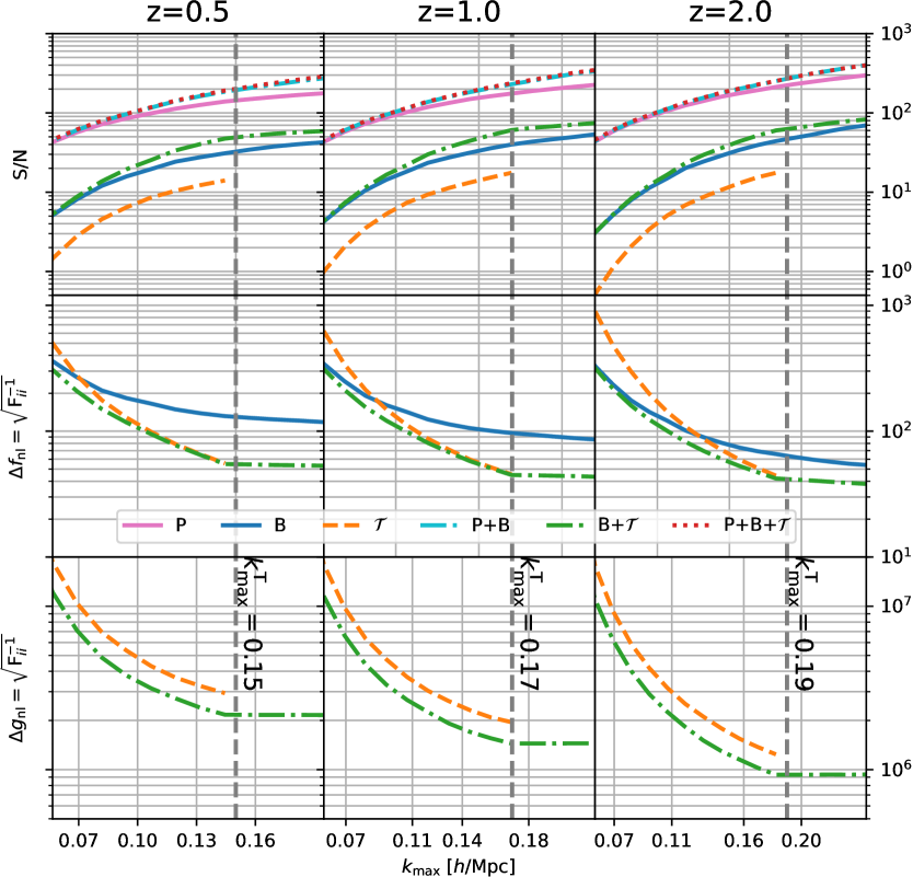
In figure 11 we show both cumulative signal-to-noise ratio (equation 2.27) and Fisher forecasts (equation 2.29) for the constraints on and as a function of for each of the redshifts considered in the analysis. The colours/line-styles are as follows: power spectrum only in magenta, bispectrum in blue, i-trispectrum in orange (dashed), joint power spectrum and bispectrum in cyan (dashed), joint bispectrum and i-trispectrum in green (dot-dashed) and full PB in red (dotted). In the cumulative signal-to-noise (top row) plots one can appreciate the increase in signal generated by adding the i-trispectrum to the bispectrum, especially in the mildly non-linear regime (as increases). Because of the logarithmic scale, it is difficult to notice the improvement when also the power spectrum is considered. The relative magnitude of the i-trispectrum effect when added to the bispectrum is similar to that observed when adding the bispectrum to the power spectrum.
Similarly, the middle row of figure 11 shows the substantial improvement obtained by using the i-trispectrum together with the bispectrum in order to constrain . We assumed in this work that the power spectrum sensitivity to and constraining power for primordial non-Gaussianity is negligible compared to bispectrum and i-trispectrum. This is because we are considering the dark matter particles as tracers. When moving to haloes this is no longer a reasonable approximation since PNG leaves a distinctive signature in the halo power spectrum through the scale dependent bias [21, 62]. Moreover the inclusion of the power spectrum would be fundamental for constraining additional cosmological or nuisance parameters, which in this analysis have been kept fixed.
Note, perhaps not unexpectedly [98], that in the very mildly non-linear regime (Mpc at ) virtually all the constraining power for comes from the i-trispectrum. Even if the bispectrum is not sensitive at the considered order in perturbation theory ( for the bispectrum) to , when used together with the i-trispectrum it helps in reducing the degeneracy present in between the two terms proportional to and (see bottom row of figure 11).
The vertical dashed lines in figure 11 mark the maximum -value used to build the quadrilaterals sets for the i-trispectrum. We considered larger -values for power spectrum and bispectrum in order to show that even if the i-trispectrum would be employed up to a lower (similarly to what happens between power spectrum and bispectrum), its effect is still significant.
Finally in table 1 we summarise these findings. The table reports values for the forecasted 1D confidence interval regions for both and . Especially at lower redshifts, adding the i-trispectrum produces constraints on that are two times tighter than the ones produced by the bispectrum alone.
The results displayed in figure 11 and table 1 are encouraging for the prospect of large scale structures surveys, such as DESI [60], which are expected to produce constraints on local primordial non-Gaussianity parameters which will be competitive and complementary to the ones obtained up now by CMB experiments such as Planck [4]. While certainly encouraging, it would be naive to conclude that these findings translate not just qualitatively but also quantitatively to realistic surveys. Real world issues such as survey geometry, galaxy bias and redshift space distortions may affect the above conclusions. In what follows, we present a first step towards more realistic estimates.
| 0.12 | 0.15 | 0.17 | 0.19 | ||||||||||
| 149 | 124 | 102 | 132 | 106 | 81 | 124 | 98 | 69 | 121 | 94 | 66 | ||
| 80 | 87 | 109 | 56 | 60 | 71 | - | 44 | 51 | - | - | 44 | ||
| 78 | 81 | 83 | 55 | 58 | 60 | 54 | 45 | 47 | 53 | 45 | 42 | ||
| 1 - | 48 | 35 | 19 | 58 | 45 | 26 | 56 | 53 | 32 | 56 | 52 | 36 | |
| 368 | 304 | 252 | 296 | 231 | 179 | - | 195 | 138 | - | - | 124 | ||
| 273 | 225 | 183 | 219 | 174 | 130 | 218 | 145 | 103 | 218 | 144 | 93 | ||
| 1 - | 14 | 12 | 11 | 19 | 17 | 16 | - | 20 | 16 | - | - | 17 | |
3.3 Redshift space
While the real space analysis presented so far indicates that in principle there is additional, useful information in the i-trispectrum, realistic observations are affected by redshift space distortions. To assess whether the real space results also hold in redshift space, in this section we present the same analysis performed on the redshift space matter density field. For this purpose, for each statistics we limit ourselves to the monopole signal only. Of course, there is potentially a lot of additional information enclosed in redshift space multipoles, but this will be presented elsewhere.
The theoretical modelling for the quantities in redshift space is presented in appendix A. Notice that, as normally done for power spectrum and bispectrum, in redshift space is corrected by a term modelling the Fingers-of-God effect (hereafter FoG) [44] (see appendix A).
We choose to focus on the redshift case, which as it can be seen from figures 5, 6 and 8, is the case where the modelling is most severely tested: the field is more non-linear and smaller error bars are derived from the measurements on simulations (compared to the cases).
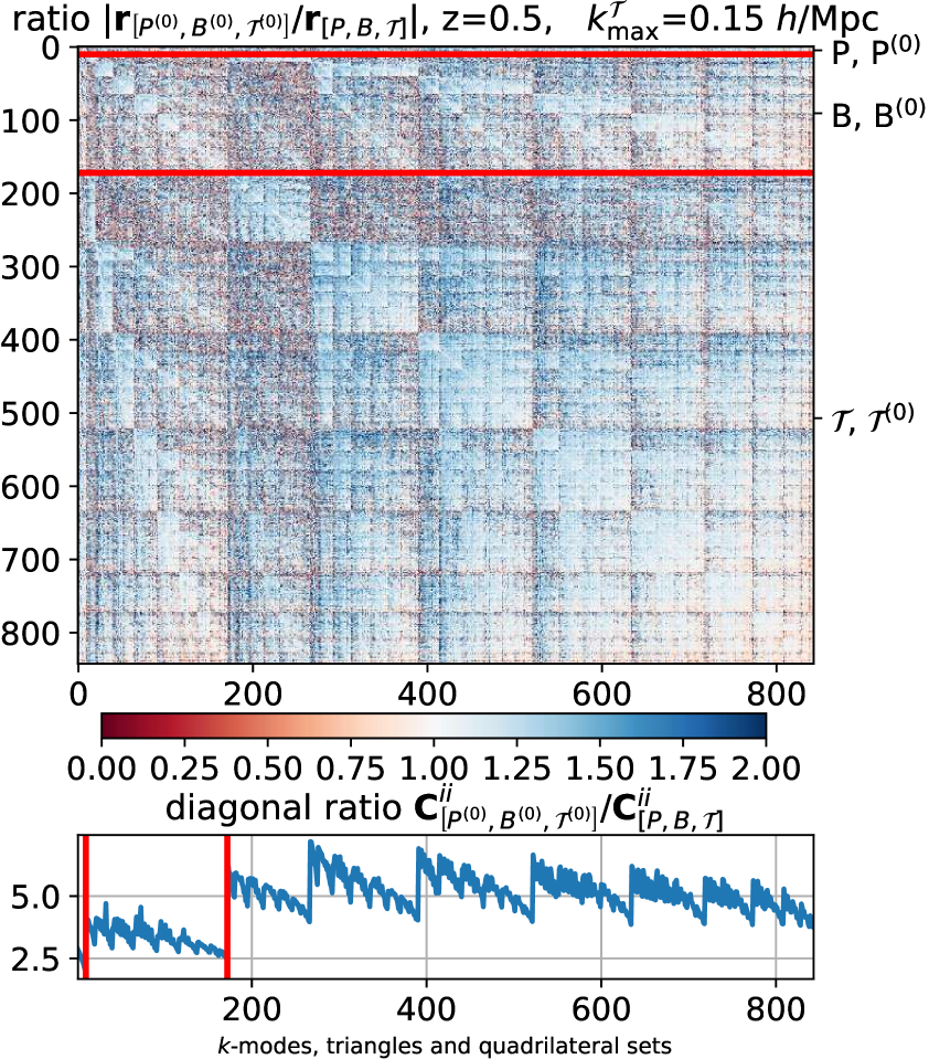
We begin by comparing the covariance matrix for the full data-vector in redshift space to the real space one. The overall structure of the redshift space matrix is very similar to that shown in the top panel of figure 9, however in details, the redshift space covariance shows more coupling between different data-vector elements. To better appreciate this, figure 12 shows the absolute value of the ratio (redshift to real space) of the elements of the reduced covariance matrices at . The off-diagonal cross-correlation between different data-vectors elements increases when the measurement is performed in redshift space, especially at the largest scales (top left region of each auto-covariance block). For the small-scales bispectrum on the other hand, the smallest scales (bottom right region of the relevant blocks) show a reduction of the cross-correlation.
We attribute this effect to two factors. First the for the bispectrum is higher than for the i-trispectrum, therefore proportionally more modes are affected by FoG effect and in the stable-clustering regime. Secondly the i-trispectrum, as it was described in section 2.1.1, is by definition an integrated quantity over many different quadrilateral shapes and hence it shows increased correlations.
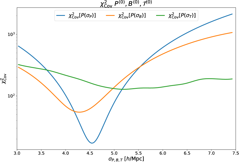
Before we can proceed to show the comparison between simulation output and theoretical modelling for the data-vector, we recall that the parameters describing the small-scales FoG damping are ultimately phenomenological parameters that must be directly fit or calibrated on N-body simulations (and possibly marginalised over).
We use a minimisation (equation 2.5) to find the values for the small-scales fingers-of-God parameters , and (equations A and A.5). This is illustrated in figure 15 in appendix A. In what follows, we adopt the values of , and that minimise the respective . These FoG parameters are kept fixed in the Fisher forecast analysis.
Figures 5 and 6 haven shown that in real space at the halofit matter power spectrum model perform better than the linear one, also as input for the bispectrum model. Therefore for all the results presented in this section we use the halofit matter power spectrum as input for computing the theoretical models. In order to obtain the best possible fit, we employ the redshift space version of the effective kernel [34] for both bispectrum and i-trispectrum models (equation A).
Figure 13 is the redshift space monopole equivalent of the panels of figures 5, 6 and 8. Together with the lines showing the models for the power spectrum, bispectrum and i-trispectrum models computed using the FoG parameters best-fit values, the models without FoG correction are also shown. As expected, the FoG term becomes more important as increases and hence in particular for power spectrum and bispectrum whose is larger than the i-trispectrum one. In the i-trispectrum case, the FoG correction helps in stabilising the ratio between model and mean of the measurements around unity for all the considered quadrilaterals sets.
The forecasted constraints for primordial non-Gaussianity parameters and their improvement when adding the i-trispectrum to the bispectrum are shown in figure 14 and reported in table 2. In the left side of figure 14 the ratio between primordial non-Gaussianity and gravitational components for both bispectrum and i-trispectrum is displayed in the redshift space case (dashed lines) and for comparison also in real space (solid line, half transparent identical colours).
Clearly the measurement in redshift space suppresses the strength of the primordial non-Gaussian component of the signal with respect to the gravitational one. This effect appears to be stronger in the i-trispectrum than for the bispectrum.
This can be understood as follows. The redshift-space distortions on large scales are gravity-driven and give a larger boost to the gravitational signal than to the PNG signal; an effect we refer to as Kaiser-boost effect. This can be easily appreciated in the left column of figure 11 where the change from real to redshift space is shown by using for the same colour both a lighter and a darker tone, respectively. Being a higher order statistic, the Kaiser-boost is naturally larger for the trispectrum than for the bispectrum as it is highlighted by the larger shift in the ratio between primordial and gravitational components. To further visualize this, in figure 17 of appendix E we focus on the Kaiser boost for equilateral configurations for both and . Because of cosmic variance, this boost also increases the errors (via the covariance matrix).
In the top-right corner of the cumulative signal-to-noise plot, the reduction in the ratio (S/N) is evident only for the i-trispectrum alone before the Mpc threshold. For the bispectrum something similar happens at smaller scales, around Mpc.
Finally the bottom right corner showing the forecasted constraints on both and , for the different statistics combinations, connects all the elements appearing in the previous results of this section regarding the measurement, modelling and forecasts in redshift space. The increased cross-correlation between different quadrilaterals sets, highlighted by the ratio between redshift and real space covariance matrices in figure 12, together with the decrease for the i-trispectrum of both the relevance of the primordial term with respect to the gravitational one and of the cumulative signal-to-noise ratio, result in a smaller impact in redshift space of the i-trispectrum in improving the constraints on both and with respect to the bispectrum alone. This is quantitatively described in table 2.
Nevertheless the improvements are still significant, reaching for a reduction of the 68 1D confidence interval when both bispectrum and i-trispectrum are employed in the analysis. The improvement for become larger as increases. This implies that improving the modelling of the signal to extend the -range to include smaller scales could return even tighter constraints on .
| , | 0.10 | 0.12 | 0.15 | 0.17 | |||||
|---|---|---|---|---|---|---|---|---|---|
| RSD (real) | RSD (real) | RSD (real) | RSD (real) | ||||||
| 194 | (183) | 157 | (149) | 135 | (132) | 125 | (124) | ||
| 240 | (136) | 153 | (80) | 117 | (56) | - | - | ||
| 164 | (122) | 118 | (78) | 91 | (55) | 88 | (54) | ||
| 1 - | 15 | (34) | 25 | (48) | 32 | (58) | 30 | (56) | |
| 1404 | (545) | 938 | (368) | 710 | (296) | - | - | ||
| 1049 | (379) | 767 | (273) | 589 | (219) | 583 | (218) | ||
| 1 - | 8 | (11) | 4 | (14) | 5 | (19) | - | - | |
4 Conclusions
In this work we have undertaken the first step towards employing the four-point correlation function’s Fourier transform, the trispectrum, in cosmological analyses of current and future galaxy clustering data-sets.
The major challenge associated to the trispectrum is its high-dimensionality: six degrees of freedom are necessary to describe a skew-quadrilateral (eight in redshift space); this makes the trispectrum algorithmically and numerically prohibitive.
We propose here to overcome this difficulty by using a compressed version of the trispectrum signal, which we refer to as the i-trispectrum. The i-trispectrum integrates the signal over all the skew-quadrilaterals defined by a set of four -modes moduli . As such, the i-trispectrum provides a solution to the trispectrum challenge by reducing the number of degrees of freedom down to four.
For the first time we model and measure the i-trispectrum both in real and redshift space. We present the i-trispectrum estimator (equation 2.16) which we then use to measure the signal from the Quijote simulations suite at different redshifts, and compare it with a theoretical model of the i-trispectrum (equation 2.1) based on perturbation theory. We find very good agreement between i-trispectrum model and measurements (figure 8) up to a maximum that, as expected, depends on redshift ( , and ).
It is important to point out that the unconnected component of the four-point correlator () must be estimated and subtracted from the total measured four-point signal to isolate the i-trispectrum. The unconnected part is far from being negligible for symmetric configurations (figure 7), and its removal is fundamental in order to isolate the the signal (i-trispectrum) containing cosmological information of the field not already present in the power spectrum.
From 5000 Quijote simulations we also estimate and present the i-trispectrum covariance matrix and its cross-correlation with power spectrum and bispectrum (figure 9). Comparing it with the simplest covariance analytical model (Gaussian field), we show that non-Gaussian and off-diagonal terms are only negligible above (figure 10). At lower redshifts, where most of the volume of present and forthcoming surveys is located, the Gaussian covariance approximation should not be used.
In analogy to the findings for the Cosmic Microwave Background anisotropies, we envisage the i-trispectrum to be particularly useful to improve the constraints on primordial non-Gaussianity (PNG) arising from lower-order statistics. We thus derive an analytical model for the local PNG signature in the i-trispectrum (equation 2.4 and figure 4), and produce realistic (using a numerically estimated covariance matrix to account for all the cross-correlations), idealized (matter field, hence low shot noise) but incomplete (non including the scale-dependent bias effect) Fisher forecasts on the PNG amplitude parameters and constraints.
In fact, additional information is indeed expected to be enclosed in the statistics of biased tracers showing the scale-dependent bias effect [21], which for the bispectrum and hence by analogy for the trispectrum, is not just present at very large scales but it is spread over many configurations [30, 96, 80].
Including the i-trispectrum in the power spectrum and bispectrum analysis has a significant impact in the resulting constraints (figure 11 and table 1). In particular, in real space the marginalised credible intervals for are approximately halved when the i-trispectrum constraining power is added to the bispectrum.
The redshift space results –monopole only– (section 3.3, figure 13) are qualitatively similar to the real space ones. However the redshift space covariance matrix shows an increased correlation between the i-trispectra of different quadrilaterals sets at the largest scales (figure 12). Only at high -values this trend inverts, possibly because of the impact of the Finger-of-God effects. This is why the i-trispectrum added value in terms of and constraints (figure 14 and table 2) is reduced compared to the real space case. Nevertheless the inclusion of the i-trispectrum provides a significant improvement on ’s 1D marginalised credible intervals.
There are some conservative aspects to our analysis, since by considering the matter field there is no scale dependent bias effect [21, 62] boosting the PNG signal. Moreover we consider a parameter space limited to the two primordial non-Gaussianity amplitudes and . It is reasonable to expect that when considering haloes/galaxies in redshift space, thus constraining a larger parameter set, the inclusion of the i-trispectrum to the data-vector can provide more significant improvements. For example the constraints on the growth rate , the bias coefficients, the amplitude of dark matter clustering , could be also significantly tightened by including the i-trispectrum. Therefore the i-trispectrum has the potential of reducing degeneracies between nuisance (e.g., galaxy bias) and cosmological parameters usually constrained by clustering analysis.
It is important to highlight that both in real and redshift space, the i-trispectrum added value becomes larger as increases. This motivates an update of the standard perturbation theory effective model [31, 34] using the i-trispectrum together with the bispectrum to fit the required parameters (Novell et al. in preparation).
The next step in order to bring the i-trispectrum into contact with real LSS data, is to model the signal of haloes or galaxies as biased tracers of the underlying dark matter field. For this we need to extend to third order the multivariate bias expansion necessary to account for the scale-dependent bias effect. This has already been done in redshift space at second order for the bispectrum [30, 7, 95, 96]. We plan to do this in future work.
An advantage of using higher-order statistics such as the bispectrum and i-trispectrum is to derive constraints on and highly complementary to CMB ones, without needing the signal from very large scales ( ) often affected by observational systematic errors, while at the same time including small scales modes. This may not be competitive for the quasars (where volume is very large but the signal to noise ratio is low), but it is interesting for emission line galaxies (ELGs) and luminous red galaxies (LRGs) which cover less volume but have higher signal to noise.
Finally, even more than for the bispectrum [36], an optimal compression algorithm will be needed in order to make it feasible to exploit the i-trispectrum full potential by using the maximum number of quadrilaterals sets allowed by the survey specifications.
We envision that, even if focused mainly on spectroscopic surveys and dark matter tracers, the estimator and the modelling presented here will be of relevance to broader sections of cosmology.
Appendix A Theoretical models for power spectrum, bispectrum and i-trispectrum
Below we report the standard perturbation theory (SPT) expressions used in the modelling of the data-vector for the analysis presented in the main text. For completeness we write the models for power spectrum, bispectrum and i-trispectrum for biased tracers in redshift space, with dependence on the orientation with respect to the line of sight ( with the angle of the -vector with respect to the line of sight). The expressions for the real space matter field are simply obtained by setting the linear bias parameter to unity in the SPT kernels while all the higher-order bias parameters together with the logarithmic growth rate parameter are set to zero. In particular, the halo power spectrum in real space is related at first order to the matter one by ; the real space expressions for the matter bispectrum are reported in the main text in equations 2.2, the real space, matter SPT expression for the i-trispectrum is given in the main text in equation 2.4. In redshift space and for biased fields we have
| (A.1) | |||||
where the redshift-space distortions kernels can be found for example in Ref. [51]’s appendix and a specific study on a more accurate bias expansion at cubic order was done by the authors of Ref. [2]. For what concerns the primordial non-Gaussianity terms reported in equation 2.4 and appendix E for matter field in real space, the equivalent redshift space expressions are obtained by simply replacing the matter field perturbation theory kernels with the redshift space ones . Notice that this can be done only for the matter field since when considering haloes or galaxies, the scale-dependent bias effect [21, 62] introduces additional non-negligible terms. As it can be seen from the above expression (see also appendix E.3), the i-trispectrum is composed of two different terms d expansions in perturbation theory up to order [28]:
| (A.2) |
The isotropic signal component –monopole– for both power spectrum and bispectrum in redshift space is given by
| (A.3) |
while the i-trispectrum monopole was defined in the main text in equation 2.7.
To model the small-scales incoherent velocity dispersion, a damping term is added for each statistics [44]. Similarly to the prescriptions used for power spectrum and bispectrum in [32] which require two effective parameters and entering the Lorentzian damping functions in front of the respective data-vectors
| (A.4) |
in the case of the i-trispectrum we use the ansatz:
| (A.5) |
The parameters , , , should be seen as effective parameters to be calibrated on simulations (or measured/marginalised over when analysing the data). In our case we find for each statistic the best-fit value of the respective FoG parameter by minimising the as in equation 2.5. The results of this procedure are displayed in figure 15 and the best-fit values are , and .
Appendix B Estimators definition
Assuming a cubic survey volume of size , the fundamental frequency is . If we divide the box into equal volume cubic cells per side, the Nyquist frequency is defined as .
Let’s recall that the first step in order to measure statistics in Fourier space from data/simulations is to grid sample the chosen tracers field by using an appropriate mass assignment scheme (see for example [82]). This returns a value of the density field at each grid-node in configuration space. From this set-up it is afterwards possible to exploit discrete Fast Fourier Transforms algorithms (FFT) [29] to obtain the Fourier transform of the density field at each node. The two grids (mass assigment and Fourier transform steps) could in principle be taken to be different but often they coincide (as in our case).
In this section we will refer to the process of converting an estimator in integral form into one written in terms of discrete sums and hence that can be applied onto a pixelated field as "pixelisation".
Using the density (matter/galaxy) perturbation variable we define the Fourier transform direct and inverse arbitrary convention:
| (B.1) |
B.1 Power spectrum
The integral version of the estimator for the power spectrum is defined as [37]
| (B.2) |
where each integral is performed over a spherical shell of radius and thickness , and . is the number of modes found inside the integration volume in Fourier space and it is defined as
| (B.3) |
In order to derive the pixelised version of the above estimator we need the Dirac’s delta expression as Fourier transform of :
| (B.4) |
Therefore in equations B.2 and B.3 we can expand the Dirac’s delta and rearrange the order of integration. Proceeding with equation B.2 by also expanding we have
Now we introduce the two quantities:
| (B.6) |
which applied to equation B.1 give,
| (B.7) |
To take advantage of fast Fourier transform techniques, each continuous integral over the whole spatial volume can be pixelised as , where is the volume of each cell. Then equation B.7 can be rewritten as,
| (B.8) |
We start by pixelising the Fourier transform of the density field :
| (B.9) |
where is the quantity computed from the Discrete Fourier Transforms algorithm (in our case FFTW [26]). Then we can proceed to pixelise both quantities in equation B.6:
| (B.10) |
where in the first step the index is used to indicate that the integrand is non-null only within the shell with radius and thickness . Hence is defined so that it is equal to unity for inside the -shell and zero outside. The normalisation factor due to the discrete inverse Fourier transform has been specified using the "IFT" subscript (inverse Fourier transform).
| (B.11) |
By construction, has the appropriate dimension of length to the power of 3.
B.2 Bispectrum
Starting from the unbiased estimator as defined in [37], for the bispectrum we have,
| (B.12) |
where , is the number of triangles included in the integration volume in Fourier space,
| (B.13) |
Proceeding then as for the power spectrum and decomposing the Dirac’s deltas using equation B.4 to derive the quantities in equation B.6 and pixelising using equation B.1 we have that
| (B.14) |
The dimension of is by construction length to the power of 6.
B.3 I-trispectrum
In analogy to the bispectrum, for the (integrated) i-trispectrum (see main text for more details) we begin by defining the unbiased estimator
where , is the number of skew-quadrilaterals in the integration volume in Fourier space, defined as
We can confirm that it is actually an unbiased estimator, as for the cases of power spectrum and bispectrum, by taking the ensemble average,
We then separately analyse the connected term and the unconnected one obtained by applying Wick’s theorem to complete the proof of the above estimator being unbiased.
B.3.1 I-trispectrum: connected part and total signal
If one considers only the connected part of the total signal estimator introduced in equation B.3, it is possible to recover the correspondence with the i-trispectrum signal
| (B.18) |
Here, as in [47], we exploited the fact that . In the last passage we assumed that if the -shell’s thickness is small enough, then after the implicit average over the possible diagonals values, can be brought outside of the integrals. Under these approximations, this connected part of the estimator is unbiased and equivalent to measuring the i-trispectrum.
Then the full four-point correlation estimator can be pixelised (again using equation B.1 for the total estimator trispectrum + unconnected part) as
From the last line of equation B.3.1 we see that also the pixelised version of the estimator has by construction dimensions of length to the power of 9.
B.3.2 Unconnected part
We now expand the unconnected part of the estimator for one of the three possible permutations:
| (B.20) |
To evaluate B.3.2 two alternatives are possible: the analytical approach or the numerical one. In the analytical approach we use the theoretical expressions for the integration volume in Fourier space for both power spectrum and i-trispectrum [39]. The analytical approach derives the theoretical result for the model of the integrated trispectrum unconnected part, since a-priori its precise form is unknown (it is expected of course to be proportional to ).
The numerical approach on the other end, proves that the estimator defined for the unconnected part of the integrated trispectrum is unbiased. In this case one can pixelise this unconnected part of the estimator as done for the connected part. In both cases the unconnected part needs to be subtracted from the measured total signal in order to obtain the i-trispectrum.
Analytical approach
We start by recalling the two expressions for the integration volumes [39]:
where is the bin-size for the -th -mode. Resuming from the last line of equation B.3.2 and assuming that, if the -shells are thin enough, the averaged value of the power spectrum does not differ significantly from the value computed at the centre of the bin, we have that
| (B.22) |
where for the case of a quadrilateral with four equal sides, . In the case of quadrilaterals sets with pairs of equal sides there is only one non-null permutation (). Given the algorithm we use to generate quadrilaterals sets (see figure 3), in our work the above only happens for example and .
A quick dimensional analysis shows that this result has the expected dimensions of length to the power of 9, the same as the connected term (trispectrum).
Numerical approach
By taking the ensemble average it is possible to check that the following estimator is unbiased with respect to the final result of the analytical approach in equation B.3.2
| (B.23) |
which we can pixelised analogously to what done for the connected part for each of the permutations:
| (B.24) |
Once again, pixelising using equation B.1, we have that the i-trispectrum unconnected part estimator becomes
| (B.25) |
The above result for the pixelised estimator corresponds to the analytical model derived in equation B.3.2.
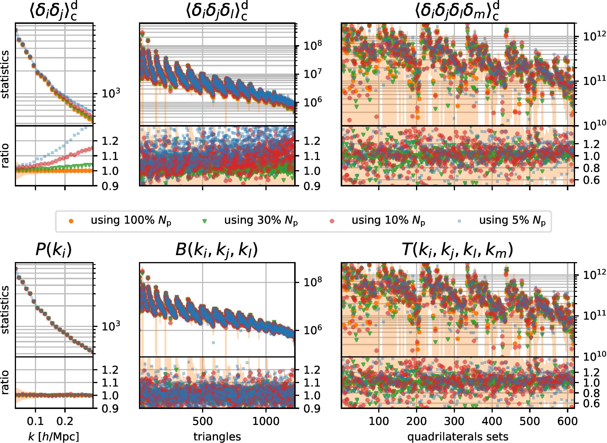
Appendix C Shot-noise correction
If the observed field is a Poisson sample of a (possibly hypothetical) continuous underlying field, the measured correlations would be affected by a shot-noise contribution which acts as a noise bias. In order to subtract the shot-noise contribution from the measured signal, we implement the suitable estimators (combinations of power spectra, bispectra and average particles density number) necessary to reproduce the terms described in the appendix of [98] under the assumption of Poissonian shot-noise. The expressions for power spectrum and bispectrum are
where the index "d" and subscript "c" stand for "discrete" and "connected", respectively and denotes the number density of objects. Notice that in this section we use the word "discrete" to indicate that the considered statistics are measured from a set of objects and not a continuous field. For the i-trispectrum, given the fact that for each set of there is an infinite number of possible quadrilateral shapes, the shot-noise expression from [98] needs to be modified. In particular for a given used to bin the -values in the measurement there is a finite number of possible values of the diagonal ranging between a and a as defined in equation 2.5, . This of course is true in the case of the shot-noise correction being estimated directly from the data. Therefore, for each of the i-trispectrum configurations defined by a set of -values , the shot-noise expression becomes,
where we used the diagonal intermediate value of each configuration’s possible range to compute the vectors sums appearing the bispectra and power spectra arguments. The terms proportional to powers of constitute the shot-noise "bias" which should be subtracted from the measured signal. Therefore these terms are first measured from the simulations and directly subtracted afterwards from the total signal measured using the estimators in equations 2.11, 2.13 and 2.2.1. Equation C is clearly an approximation, a more rigorous treatment would involve averaging the above terms over all the possible values of the diagonal . We tested this and found no significant change. Most likely this is due to the fact the i-trispectrum measurement is dominated by statistical noise as it can be seen from figure 16. Notice that the term for the closure condition, and therefore does not need to be averaged.
Figure 16 shows the increase in relevance of the shot-noise term as the number of tracers decreases. For one realisation at , the dark matter particles present in the cubic box have been randomly sampled to include , , and of the total. In the upper half of the figure shows the corresponding discrete power spectrum, bispectrum and connected part of the i-trispectrum, measured using the estimators in equations 2.11, 2.13, 2.16. In the lower half the same cases have been shown for the statistics of interest obtained subtracting the shot-noise terms as described in equations C and C.
Without shot-noise correction a significant bias would be induced in both power spectrum and bispectrum measurements, especially at large -values. The relevance of this bias is given by its comparison with the error bars derived from the set of measurements on the simulations. For the i-trispectrum, even when decreasing the number of samples down to of the original set, the induced shift in the statistics is still smaller than the error bars. The shot-noise correction does not have an impact as significative as in the case of power spectrum and bispectrum because of the dominant sample variance error. In other words, the large statistical error associated with measuring the i-trispectrum from a less dense catalogue of tracers dominates over the shot-noise effect, at least up to the considered in this work.
Appendix D I-trispectrum covariance: Gaussian term in redshift space
Using the estimator defined in equation 2.16, the covariance matrix for the tracer field (halo or galaxy) i-trispectrum in redshift space is given by:
| (D.1) | |||||
where we used the approximation made in [47] that ; denotes the redshift space tracer (halo or galaxy) power spectrum, is the survey volume and the fundamental frequency; is a symmetry factor that counts the number of possible combinations of equal sides between the two identical quadrilaterals sets. Depending on the number of equal sides, assumes the values:
| (D.2) |
Appendix E Primordial non-Gaussianity
We recap here the formalism presented in the appendix of Ref. [36] for both power spectrum and bispectrum and extend it to include the i-trispectrum for the matter field in real space (replace the SPT kernels with the redshift space ones in appendix A for the redshift space case).
For the three statistics (power spectrum, bispectrum and i-trispectrum) we compute the contribution due to the presence of a primordial non-Gaussian component of the local type in the potential field. The primordial (subscript p) potential (which in our work has units of in order for equation E.6 appearing later to be dimensionless) can be thus parametrised as:
| (E.1) |
where represents a Gaussian field. In Fourier space it translates to:
| (E.2) |
where in Fourier space , and denotes the Fourier transform of and denotes the power spectrum of the field. In order to write in a compact way we write for different quantities the argument as a subscript (e.g., or ). For the same reason to express many integrals appearing in the perturbation expansion we have introduced the short notation:
Late-time and primordial potentials are related by:
| (E.4) |
where the operator describing the full non-linear evolution of the primordial field has been linearised in the last step, is the linear growth factor as a function of the scale factor and is the transfer function. At late-times the potential field is related to the density perturbation variable by the Poisson equation:
| (E.5) |
This allows us to link the primordial potential with the late-time matter density perturbation assuming, as normally done in the literature, that only the linearly evolved component of the primordial (potentially including non-Gaussianities) field sources the late time gravitational potential .:
| (E.6) |
In the rest of this appendix, to use a more compact notation, the wave-vector or wave-number in the argument is reported as a subscript index.
E.1 Power spectrum
As described in [36] up to order for the matter power spectrum we have the terms:
| (E.7) |
The first term is given by
where and we include it to simplify the transformation to the matter redshift space expressions, where . Notice that the integral in the second term proportional to is divergent for . However these integrals should be performed for a corresponding to the size of the causally connected patch of the Universe and therefore it is effectively a finite quantity.
The second term, , reads
The other terms in the power spectrum expansion, and , are at first order already proportional to and therefore in our case they just return the standard terms for the Gaussian initial conditions.
E.2 Bispectrum
Limiting the expansion in terms of the Gaussian primordial potential up to order , as described in [36]’s appendix, for the bispectrum there is only a primordial term together with the standard one due to gravitational collapse. The expression for is given by
where in the last line the primordial power spectrum was converted into the late-time matter power spectrum.
E.3 Trispectrum
The terms we report here were presented (in a less padagogical way) in [46] and [79]. In this subsection, for clarity and self-consistency, we also report them using a notation consistent with the rest of the paper. In the case of i-trispectrum, primordial corrections appear at order at the lowest order in . By converting into the late time matter perturbation density variable , it can be noticed that this is the same order of the standard gravitational term for Gaussian initial conditions. It is indeed the lowest order at which the connected part of the four-point correlation function in Fourier Space appears. Therefore we will consider only terms of order . Proceeding as before:
| (E.11) |
The i-trispectrum corresponding to Gaussian initial conditions is given by terms and . Without PNG, would represent the unconnected part of the four-point correlator in Fourier space. However expanding in terms of PNG results in non-trivial terms proportional to both and . Finally would be zero for Gaussian initial conditions since it is an odd moment. However with PNG, up to order it will produce at least one term proportional to .
We will follow the approach of first expanding each expression in terms of late-time density perturbation variables and then express each of these in terms of early time potential field using equation E.6. Finally we will convert to its expansion in terms of the early-time Gaussian potential using equation E.2.
E.3.1
| (E.12) |
We then have two kind of PNG-dependent terms, one proportional to and one to :
Given the several permutations let us split this computation in two terms proportional to the two PNG parameters. Proceeding with the first, , we can see that the six-point correlator can be decomposed in the following terms:
| (E.14) |
The symmetry factors are due to permutations over the auxiliary variables. Only the last term is fully connected, therefore we expect the others to be cancelled out by the other three terms appearing in the expression for . Let us find out:
From the last line we can see that one term did not cancel out (first one). However this represents (as it can be seen from the Dirac’s deltas) an unconnected part of the four-point correlation function. It is indeed the primordial contribution to the power spectrum reported in equation E.1.
From the Dirac deltas appearing in the above computation we also notice that for first part of the connected term , , and . For the second one we have the relations , , and .
We can now focus on the other term, :
| (E.16) |
The first term can be easily spotted to be unconnected and should cancel out:
| (E.17) |
From the Dirac deltas appearing in the above computation we also notice that for the connected term , and .
Basically the PNG terms and are respectively the equivalent of the terms and for the Gaussian initial condition due to gravitational non-linear evolution.
As last step we express the above result in terms of the late-time matter power spectrum using equation E.6.
E.3.2
This is perhaps the most interesting PNG term of the i-trispectrum, since. as for the bispectrum, it comes from a correlator that would be null for Gaussian initial conditions.
There are two possible terms proportional to from the above expansion. The first corresponds to the associated to a , the second to that associated to .
| (E.21) |
where the two permutations in the second line correspond to expanding or instead of . Proceed step by step we now analyse the two terms separately, namely and . Starting from the first:
| (E.22) |
In order to proceed as generally as possible, we need to separately treat the combinations arising from the mixing between original wave vectors with auxiliary ones originating from different sources (equation E.3.2).
The constant derives from the second order kernel including redshift space distortions in the case of opposite -vectors. Only the term in the second line represents a connected part of the initial four-point correlator. From the Dirac deltas resulting in the connected part we can notice that and . This is a clear example of mode coupling between non-linear evolution and primordial non-Gaussian initial conditions. Moving to the second term :
| (E.24) |
Which then expanded becomes:
where all the permutations above consist in changing with either or . Only the second term represents a connected part of the initial four-point correlator. From the Dirac deltas resulting in the connected part we can notice that and . We can now proceed with equation E.3.2, using only the connected terms from and :
As a final step we can convert the above result into an expression in terms of the late-time matter power spectrum using equation E.6
It is better to not further regroup together the two terms since the number of possible permutations is different.
We conclude this i-trispectrum calculation by recalling that up to order the two remaining terms and return only the standard expression.
E.4 Recap: all PNG terms
Power Spectrum
Bispectrum
| (E.29) |
Trispectrum
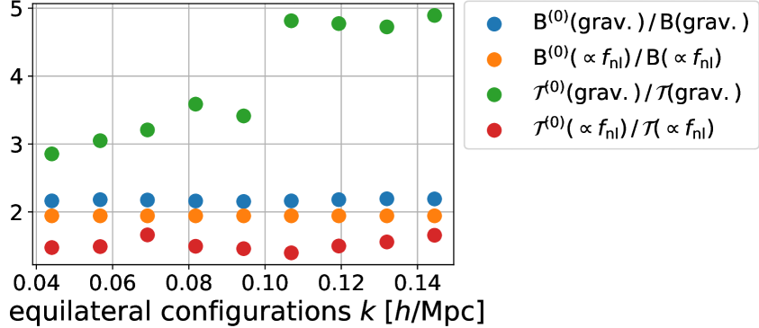
Acknowledgments
D.G. and L.V. thank Francisco Villaescusa-Navarro for invaluable help with the extensive use of the Quijote simulations. D.G. is grateful to Nicola Bellomo and Alex Mead for useful discussions. All authors wish to thank the anonymous referee for the very constructive referee report which improved the paper’s presentation.
The measurements from the simulations were performed in the TigerCPU cluster at Princeton. L.V. and D.G. acknowledge support of European Unions Horizon 2020 research and innovation programme ERC (BePreSySe, grant agreement 725327). Funding for this work was partially provided by the Spanish MINECO under projects PGC2018-098866-B-I00 FEDER-EU.
HGM acknowledges the support from ‘la Caixa’ Foundation (ID100010434) with code
LCF/BQ/PI18/11630024.
References
- [1] Paul A. Abell et al. LSST Science Book, Version 2.0. 2009.
- [2] Muntazir Mehdi Abidi and Tobias Baldauf. Cubic Halo Bias in Eulerian and Lagrangian Space. JCAP, 07:029, 2018.
- [3] Nishant Agarwal, Vincent Desjacques, Donghui Jeong, and Fabian Schmidt. Information content in the redshift-space galaxy power spectrum and bispectrum. 7 2020.
- [4] Y. Akrami et al. Planck 2018 results. IX. Constraints on primordial non-Gaussianity. 2019.
- [5] Justin Alsing, Tom Charnock, Stephen Feeney, and Benjamin Wand elt. Fast likelihood-free cosmology with neural density estimators and active learning. MNRAS, 488(3):4440–4458, September 2019.
- [6] David J. Bacon et al. Cosmology with Phase 1 of the Square Kilometre Array: Red Book 2018: Technical specifications and performance forecasts. Submitted to: Publ. Astron. Soc. Austral., 2018.
- [7] Tobias Baldauf, Uros Seljak, and Leonardo Senatore. Primordial non-Gaussianity in the Bispectrum of the Halo Density Field. JCAP, 1104:006, 2011.
- [8] James M. Bardeen. Gauge Invariant Cosmological Perturbations. Phys. Rev., D22:1882–1905, 1980.
- [9] Alexandre Barreira. On the impact of galaxy bias uncertainties on primordial non-Gaussianity constraints. 9 2020.
- [10] N. Bartolo, E. Komatsu, Sabino Matarrese, and A. Riotto. Non-Gaussianity from inflation: Theory and observations. Phys. Rept., 402:103–266, 2004.
- [11] Nicola Bellomo, Nicola Bartolo, Raul Jimenez, Sabino Matarrese, and Licia Verde. Measuring the Energy Scale of Inflation with Large Scale Structures. JCAP, 11:043, 2018.
- [12] Daniele Bertolini, Katelin Schutz, Mikhail P. Solon, and Kathryn M. Zurek. The Trispectrum in the Effective Field Theory of Large Scale Structure. JCAP, 06:052, 2016.
- [13] Simeon Bird, Matteo Viel, and Martin G. Haehnelt. Massive Neutrinos and the Non-linear Matter Power Spectrum. Mon. Not. Roy. Astron. Soc., 420:2551–2561, 2012.
- [14] Julien Carron. On the assumption of Gaussianity for cosmological two-point statistics and parameter dependent covariance matrices. Astron. Astrophys., 551:A88, 2013.
- [15] Emanuele Castorina et al. Redshift-weighted constraints on primordial non-Gaussianity from the clustering of the eBOSS DR14 quasars in Fourier space. JCAP, 09:010, 2019.
- [16] Kwan Chuen Chan and Linda Blot. Assessment of the Information Content of the Power Spectrum and Bispectrum. Phys. Rev. D, 96(2):023528, 2017.
- [17] Planck Collaboration, N. Aghanim, Y. Akrami, M. Ashdown, J. Aumont, C. Baccigalupi, M. Ballardini, A. J. Banday, R. B. Barreiro, N. Bartolo, S. Basak, R. Battye, K. Benabed, J. P. Bernard, M. Bersanelli, P. Bielewicz, J. J. Bock, J. R. Bond, J. Borrill, F. R. Bouchet, F. Boulanger, M. Bucher, C. Burigana, R. C. Butler, E. Calabrese, J. F. Cardoso, J. Carron, A. Challinor, H. C. Chiang, J. Chluba, L. P. L. Colombo, C. Combet, D. Contreras, B. P. Crill, F. Cuttaia, P. de Bernardis, G. de Zotti, J. Delabrouille, J. M. Delouis, E. Di Valentino, J. M. Diego, O. Doré, M. Douspis, A. Ducout, X. Dupac, S. Dusini, G. Efstathiou, F. Elsner, T. A. Enßlin, H. K. Eriksen, Y. Fantaye, M. Farhang, J. Fergusson, R. Fernandez-Cobos, F. Finelli, F. Forastieri, M. Frailis, A. A. Fraisse, E. Franceschi, A. Frolov, S. Galeotta, S. Galli, K. Ganga, R. T. Génova-Santos, M. Gerbino, T. Ghosh, J. González-Nuevo, K. M. Górski, S. Gratton, A. Gruppuso, J. E. Gudmundsson, J. Hamann, W. Handley, F. K. Hansen, D. Herranz, S. R. Hildebrandt, E. Hivon, Z. Huang, A. H. Jaffe, W. C. Jones, A. Karakci, E. Keihänen, R. Keskitalo, K. Kiiveri, J. Kim, T. S. Kisner, L. Knox, N. Krachmalnicoff, M. Kunz, H. Kurki-Suonio, G. Lagache, J. M. Lamarre, A. Lasenby, M. Lattanzi, C. R. Lawrence, M. Le Jeune, P. Lemos, J. Lesgourgues, F. Levrier, A. Lewis, M. Liguori, P. B. Lilje, M. Lilley, V. Lindholm, M. López-Caniego, P. M. Lubin, Y. Z. Ma, J. F. Macías-Pérez, G. Maggio, D. Maino, N. Mandolesi, A. Mangilli, A. Marcos-Caballero, M. Maris, P. G. Martin, M. Martinelli, E. Martínez-González, S. Matarrese, N. Mauri, J. D. McEwen, P. R. Meinhold, A. Melchiorri, A. Mennella, M. Migliaccio, M. Millea, S. Mitra, M. A. Miville-Deschênes, D. Molinari, L. Montier, G. Morgante, A. Moss, P. Natoli, H. U. Nørgaard-Nielsen, L. Pagano, D. Paoletti, B. Partridge, G. Patanchon, H. V. Peiris, F. Perrotta, V. Pettorino, F. Piacentini, L. Polastri, G. Polenta, J. L. Puget, J. P. Rachen, M. Reinecke, M. Remazeilles, A. Renzi, G. Rocha, C. Rosset, G. Roudier, J. A. Rubiño-Martín, B. Ruiz-Granados, L. Salvati, M. Sandri, M. Savelainen, D. Scott, E. P. S. Shellard, C. Sirignano, G. Sirri, L. D. Spencer, R. Sunyaev, A. S. Suur-Uski, J. A. Tauber, D. Tavagnacco, M. Tenti, L. Toffolatti, M. Tomasi, T. Trombetti, L. Valenziano, J. Valiviita, B. Van Tent, L. Vibert, P. Vielva, F. Villa, N. Vittorio, B. D. Wandelt, I. K. Wehus, M. White, S. D. M. White, A. Zacchei, and A. Zonca. Planck 2018 results. vi. cosmological parameters, 2018.
- [18] Asantha Cooray, Chao Li, and Alessandro Melchiorri. The trispectrum of 21-cm background anisotropies as a probe of primordial non-Gaussianity. Phys. Rev. D, 77:103506, 2008.
- [19] Paolo Creminelli and Matias Zaldarriaga. Single field consistency relation for the 3-point function. JCAP, 10:006, 2004.
- [20] M. Crocce, S. Pueblas, and R. Scoccimarro. Transients from Initial Conditions in Cosmological Simulations. Mon. Not. Roy. Astron. Soc., 373:369–381, 2006.
- [21] Neal Dalal, Olivier Dore, Dragan Huterer, and Alexander Shirokov. The imprints of primordial non-gaussianities on large-scale structure: scale dependent bias and abundance of virialized objects. Phys. Rev. D, 77:123514, 2008.
- [22] G. de Troia, P. A. R. Ade, J. J. Bock, J. R. Bond, A. Boscaleri, C. R. Contaldi, B. P. Crill, P. de Bernardis, P. G. Ferreira, M. Giacometti, E. Hivon, V. V. Hristov, M. Kunz, A. E. Lange, S. Masi, P. D. Mauskopf, T. Montroy, P. Natoli, C. B. Netterfield, E. Pascale, F. Piacentini, G. Polenta, G. Romeo, and J. E. Ruhl. The trispectrum of the cosmic microwave background on subdegree angular scales: an analysis of the BOOMERanG data. Monthly Notices of the Royal Astronomical Society, 343(1):284–292, 07 2003.
- [23] Richard Ellis et al. Extragalactic science, cosmology, and Galactic archaeology with the Subaru Prime Focus Spectrograph. Publ. Astron. Soc. Jap., 66(1):R1, 2014.
- [24] Chang Feng, Asantha Cooray, Joseph Smidt, Jon O’Bryan, Brian Keating, and Donough Regan. Planck Trispectrum Constraints on Primordial Non-Gaussianity at Cubic Order. Phys. Rev. D, 92(4):043509, 2015.
- [25] J.R. Fergusson, D.M. Regan, and E.P.S. Shellard. Optimal Trispectrum Estimators and WMAP Constraints. 12 2010.
- [26] Matteo Frigo and Steven~G. Johnson. The Design and Implementation of {FFTW3}. Proceedings of the IEEE, 93(2):216–231, 2005.
- [27] J. N. Fry and P. J. E. Peebles. Statistical analysis of catalogs of extragalactic objects. IX. The four-point galaxy correlation function. ApJ, 221:19–33, April 1978.
- [28] James N. Fry. The Galaxy correlation hierarchy in perturbation theory. Astrophys. J., 279:499–510, 1984.
- [29] W. M. Gentleman and G. Sande. Fast fourier transforms: For fun and profit. In Proceedings of the November 7-10, 1966, Fall Joint Computer Conference, AFIPS ’66 (Fall), page 563–578, New York, NY, USA, 1966. Association for Computing Machinery.
- [30] Tommaso Giannantonio and Cristiano Porciani. Structure formation from non-Gaussian initial conditions: multivariate biasing, statistics, and comparison with N-body simulations. Phys. Rev. D, 81:063530, 2010.
- [31] Hector Gil-Marin, Christian Wagner, Frantzeska Fragkoudi, Raul Jimenez, and Licia Verde. An improved fitting formula for the dark matter bispectrum. JCAP, 02:047, 2012.
- [32] Héctor Gil-Marín, Jorge Noreña, Licia Verde, Will J. Percival, Christian Wagner, Marc Manera, and Donald P. Schneider. The power spectrum and bispectrum of SDSS DR11 BOSS galaxies – I. Bias and gravity. Mon. Not. Roy. Astron. Soc., 451(1):539–580, 2015.
- [33] Héctor Gil-Marín, Will J. Percival, Licia Verde, Joel R. Brownstein, Chia-Hsun Chuang, Francisco-Shu Kitaura, Sergio A. Rodríguez-Torres, and Matthew D. Olmstead. The clustering of galaxies in the SDSS-III Baryon Oscillation Spectroscopic Survey: RSD measurement from the power spectrum and bispectrum of the DR12 BOSS galaxies. Mon. Not. Roy. Astron. Soc., 465(2):1757–1788, 2017.
- [34] Héctor Gil-Marín, Christian Wagner, Jorge Noreña, Licia Verde, and Will Percival. Dark matter and halo bispectrum in redshift space: theory and applications. JCAP, 12:029, 2014.
- [35] J. Green et al. Wide-Field InfraRed Survey Telescope (WFIRST) Final Report. 8 2012.
- [36] Davide Gualdi, Héctor Gil-Marín, Marc Manera, Benjamin Joachimi, and Ofer Lahav. GEOMAX: beyond linear compression for 3pt galaxy clustering statistics. 12 2019.
- [37] Davide Gualdi, Héctor Gil-Marín, Robert L. Schuhmann, Marc Manera, Benjamin Joachimi, and Ofer Lahav. Enhancing BOSS bispectrum cosmological constraints with maximal compression. Mon. Not. Roy. Astron. Soc., 484(3):3713–3730, 2019.
- [38] Davide Gualdi, Marc Manera, Benjamin Joachimi, and Ofer Lahav. Maximal compression of the redshift space galaxy power spectrum and bispectrum. Mon. Not. Roy. Astron. Soc., 476(3):4045–4070, 2018.
- [39] Davide Gualdi and Licia Verde. Galaxy redshift-space bispectrum: the Importance of Being Anisotropic. JCAP, 06:041, 2020.
- [40] ChangHoon Hahn, Francisco Villaescusa-Navarro, Emanuele Castorina, and Roman Scoccimarro. Constraining with the bispectrum. Part I. Breaking parameter degeneracies. JCAP, 03:040, 2020.
- [41] A. J. S. Hamilton. Linear redshift distortions: A Review. In Ringberg Workshop on Large Scale Structure Ringberg, Germany, September 23-28, 1996, 1997.
- [42] J. Hartlap, Patrick Simon, and P. Schneider. Why your model parameter confidences might be too optimistic: Unbiased estimation of the inverse covariance matrix. Astron. Astrophys., 464:399, 2007.
- [43] Keisuke Izumi, Shuntaro Mizuno, and Kazuya Koyama. Trispectrum estimation in various models of equilateral type non-Gaussianity. Phys. Rev. D, 85:023521, 2012.
- [44] J. C. Jackson. Fingers of God: A critique of Rees’ theory of primoridal gravitational radiation. Mon. Not. Roy. Astron. Soc., 156:1P–5P, 1972.
- [45] Donghui Jeong. Cosmology with high (z>1) redshift galaxy surveys. PhD thesis, University of Texas at Austin, August 2010.
- [46] Donghui Jeong and Eiichiro Komatsu. Primordial non-Gaussianity, scale-dependent bias, and the bispectrum of galaxies. Astrophys. J., 703:1230–1248, 2009.
- [47] B. Joachimi, X. Shi, and P. Schneider. Bispectrum covariance in the flat-sky limit. Astron. Astrophys., 508:1193, 2009.
- [48] N. Kaiser. Clustering in real space and in redshift space. Mon. Not. Roy. Astron. Soc., 227:1–27, 1987.
- [49] B. Kalus, W.J. Percival, and L. Samushia. Cosmological parameter inference from galaxy clustering: The effect of the posterior distribution of the power spectrum. Mon. Not. Roy. Astron. Soc., 455(3):2573–2581, 2016.
- [50] Marc Kamionkowski, Tristan L. Smith, and Alan Heavens. The CMB Bispectrum, Trispectrum, non-Gaussianity, and the Cramer-Rao Bound. Phys. Rev. D, 83:023007, 2011.
- [51] Dionysios Karagiannis, Andrei Lazanu, Michele Liguori, Alvise Raccanelli, Nicola Bartolo, and Licia Verde. Constraining primordial non-Gaussianity with bispectrum and power spectrum from upcoming optical and radio surveys. Mon. Not. Roy. Astron. Soc., 478(1):1341–1376, 2018.
- [52] Eiichiro Komatsu. The pursuit of non-gaussian fluctuations in the cosmic microwave background. PhD thesis, Tohoku U., 2001.
- [53] Eiichiro Komatsu and David N. Spergel. Acoustic signatures in the primary microwave background bispectrum. Phys. Rev., D63:063002, 2001.
- [54] M. Kunz, A. J. Banday, P. G. Castro, P. G. Ferreira, and K. M. Górski. The Trispectrum of the 4 Year COBE DMR Data. ApJ, 563(2):L99–L102, December 2001.
- [55] R. Laureijs et al. Euclid Definition Study Report. 2011.
- [56] Titouan Lazeyras, Marcello Musso, and Vincent Desjacques. Lagrangian bias of generic large-scale structure tracers. Phys. Rev. D, 93(6):063007, 2016.
- [57] Titouan Lazeyras and Fabian Schmidt. Beyond LIMD bias: a measurement of the complete set of third-order halo bias parameters. JCAP, 09:008, 2018.
- [58] Hayden Lee and Cora Dvorkin. Cosmological Angular Trispectra and Non-Gaussian Covariance. JCAP, 05:044, 2020.
- [59] Julien Lesgourgues. The Cosmic Linear Anisotropy Solving System (CLASS) I: Overview. 4 2011.
- [60] M. Levi, C. Bebek, T. Beers, R. Blum, R. Cahn, D. Eisenstein, B. Flaugher, K. Honscheid, R. Kron, O. Lahav, P. McDonald, N. Roe, D. Schlegel, and representing the DESI collaboration. The DESI Experiment, a whitepaper for Snowmass 2013. ArXiv e-prints, August 2013.
- [61] Juan Martin Maldacena. Non-Gaussian features of primordial fluctuations in single field inflationary models. JHEP, 05:013, 2003.
- [62] Sabino Matarrese and Licia Verde. The effect of primordial non-Gaussianity on halo bias. Astrophys. J. Lett., 677:L77–L80, 2008.
- [63] Alexander Mead, Catherine Heymans, Lucas Lombriser, John Peacock, Olivia Steele, and Hans Winther. Accurate halo-model matter power spectra with dark energy, massive neutrinos and modified gravitational forces. Mon. Not. Roy. Astron. Soc., 459(2):1468–1488, 2016.
- [64] Shuntaro Mizuno and Kazuya Koyama. Trispectrum estimator in equilateral type non-Gaussian models. JCAP, 10:002, 2010.
- [65] Irshad Mohammed, Uros Seljak, and Zvonimir Vlah. Perturbative approach to covariance matrix of the matter power spectrum. Mon. Not. Roy. Astron. Soc., 466(1):780–797, 2017.
- [66] Dipak Munshi, Alan Heavens, Asantha Cooray, Joseph Smidt, Peter Coles, and Paolo Serra. New Optimised Estimators for the Primordial Trispectrum. Mon. Not. Roy. Astron. Soc., 412:1993, 2011.
- [67] Toshiya Namikawa. Constraints on Patchy Reionization from Planck CMB Temperature Trispectrum. Phys. Rev. D, 97(6):063505, 2018.
- [68] Toshiya Namikawa. Constraints on patchy reionization from Planck CMB temperature trispectrum. Phys. Rev. D, 97(6):063505, March 2018.
- [69] P. J. E. Peebles. The large-scale structure of the universe. 1980.
- [70] J. Pielorz, J. Rödiger, I. Tereno, and P. Schneider. A fitting formula for the non-Gaussian contribution to the lensing power spectrum covariance. A&A, 514:A79, May 2010.
- [71] Doogesh Kodi Ramanah, Guilhem Lavaux, Jens Jasche, and Benjamin D. Wand elt. Cosmological inference from Bayesian forward modelling of deep galaxy redshift surveys. A&A, 621:A69, January 2019.
- [72] Donough Regan, Mateja Gosenca, and David Seery. Constraining the WMAP9 bispectrum and trispectrum with needlets. Journal of Cosmology and Astroparticle Physics, 2015(01):013–013, jan 2015.
- [73] Cristiano G. Sabiu, Ben Hoyle, Juhan Kim, and Xiao-Dong Li. Graph Database Solution for Higher Order Spatial Statistics in the Era of Big Data. Astrophys. J. Suppl., 242(2):29, 2019.
- [74] Roman Scoccimarro. The bispectrum: from theory to observations. Astrophys. J., 544:597, 2000.
- [75] Roman Scoccimarro. Fast Estimators for Redshift-Space Clustering. Phys. Rev. D, 92(8):083532, 2015.
- [76] Román Scoccimarro, Hume A. Feldman, J. N. Fry, and Joshua A. Frieman. The Bispectrum of IRAS Redshift Catalogs. ApJ, 546(2):652–664, January 2001.
- [77] Roman Scoccimarro, Lam Hui, Marc Manera, and Kwan Chuen Chan. Large-scale Bias and Efficient Generation of Initial Conditions for Non-Local Primordial Non-Gaussianity. Phys. Rev. D, 85:083002, 2012.
- [78] Roman Scoccimarro, Emiliano Sefusatti, and Matias Zaldarriaga. Probing primordial non-Gaussianity with large - scale structure. Phys. Rev., D69:103513, 2004.
- [79] Emiliano Sefusatti. 1-loop Perturbative Corrections to the Matter and Galaxy Bispectrum with non-Gaussian Initial Conditions. Phys. Rev. D, 80:123002, 2009.
- [80] Emiliano Sefusatti, Martin Crocce, and Vincent Desjacques. The Halo Bispectrum in N-body Simulations with non-Gaussian Initial Conditions. Mon. Not. Roy. Astron. Soc., 425:2903, 2012.
- [81] Emiliano Sefusatti, Martin Crocce, Sebastian Pueblas, and Roman Scoccimarro. Cosmology and the Bispectrum. Phys. Rev. D, 74:023522, 2006.
- [82] Emiliano Sefusatti, Martin Crocce, Roman Scoccimarro, and Hugh Couchman. Accurate Estimators of Correlation Functions in Fourier Space. Mon. Not. Roy. Astron. Soc., 460(4):3624–3636, 2016.
- [83] Emiliano Sefusatti and Roman Scoccimarro. Galaxy bias and halo-occupation numbers from large-scale clustering. Phys. Rev. D, 71:063001, 2005.
- [84] Elena Sellentin and Alan F. Heavens. Parameter inference with estimated covariance matrices. Mon. Not. Roy. Astron. Soc., 456(1):L132–L136, 2016.
- [85] Kendrick M. Smith, Leonardo Senatore, and Matias Zaldarriaga. Optimal analysis of the CMB trispectrum. 2 2015.
- [86] R.E. Smith, J.A. Peacock, A. Jenkins, S.D.M. White, C.S. Frenk, F.R. Pearce, P.A. Thomas, G. Efstathiou, and H.M.P. Couchmann. Stable clustering, the halo model and nonlinear cosmological power spectra. Mon. Not. Roy. Astron. Soc., 341:1311, 2003.
- [87] Volker Springel and Lars Hernquist. Cosmological SPH simulations: A Hybrid multi-phase model for star formation. Mon. Not. Roy. Astron. Soc., 339:289, 2003.
- [88] Naonori S. Sugiyama, Shun Saito, Florian Beutler, and Hee-Jong Seo. A complete FFT-based decomposition formalism for the redshift-space bispectrum. Mon. Not. Roy. Astron. Soc., 484(1):364–384, 2019.
- [89] Naonori S. Sugiyama, Shun Saito, Florian Beutler, and Hee-Jong Seo. Perturbation theory approach to predict the covariance matrices of the galaxy power spectrum and bispectrum in redshift space. 8 2019.
- [90] Yasushi Suto and Takahiko Matsubara. Departure from hierarchical clustering relations for two, three, and four point correlation functions: Analysis of cosmological N body simulations. 3 1993.
- [91] Ryuichi Takahashi, Masanori Sato, Takahiro Nishimichi, Atsushi Taruya, and Masamune Oguri. Revising the Halofit Model for the Nonlinear Matter Power Spectrum. Astrophys. J., 761:152, 2012.
- [92] Atsushi Taruya, Takahiro Nishimichi, and Donghui Jeong. The covariance of the matter power spectrum including the survey window function effect: N-body simulations vs. fifth-order perturbation theory on grid. 7 2020.
- [93] Peter L. Taylor, Thomas D. Kitching, Justing Alsing, Benjamin D. Wandelt, Stephen M. Feeney, and Jason D. McEwen. Cosmic shear: Inference from forward models. Phys. Rev. D, 100(2):023519, July 2019.
- [94] Max Tegmark, Andy Taylor, and Alan Heavens. Karhunen-Loeve eigenvalue problems in cosmology: How should we tackle large data sets? Astrophys. J., 480:22, 1997.
- [95] Matteo Tellarini, Ashley J. Ross, Gianmassimo Tasinato, and David Wands. Non-local bias in the halo bispectrum with primordial non-Gaussianity. JCAP, 07:004, 2015.
- [96] Matteo Tellarini, Ashley J. Ross, Gianmassimo Tasinato, and David Wands. Galaxy bispectrum, primordial non-Gaussianity and redshift space distortions. JCAP, 06:014, 2016.
- [97] Joseph Tomlinson, Donghui Jeong, and Juhan Kim. Efficient parallel algorithm for estimating higher-order polyspectra. Astron. J., 158(3):116, 2019.
- [98] Licia Verde and Alan F. Heavens. On the trispectrum as a Gaussian test for cosmology. Astrophys. J., 553:14, 2001.
- [99] Licia Verde, Alan F. Heavens, Will J. Percival, Sabino Matarrese, Carlton M. Baugh, Joss Bland-Hawthorn, Terry Bridges, Russell Cannon, Shaun Cole, Matthew Colless, Chris Collins, Warrick Couch, Gavin Dalton, Roberto De Propris, Simon P. Driver, George Efstathiou, Richard S. Ellis, Carlos S. Frenk, Karl Glazebrook, Carole Jackson, Ofer Lahav, Ian Lewis, Stuart Lumsden, Steve Maddox, Darren Madgwick, Peder Norberg, John A. Peacock, Bruce A. Peterson, Will Sutherland, and Keith Taylor. The 2dF Galaxy Redshift Survey: the bias of galaxies and the density of the Universe. MNRAS, 335(2):432–440, September 2002.
- [100] Licia Verde, Li-Min Wang, Alan Heavens, and Marc Kamionkowski. Large scale structure, the cosmic microwave background, and primordial non-gaussianity. Mon. Not. Roy. Astron. Soc., 313:L141–L147, 2000.
- [101] Francisco Villaescusa-Navarro et al. The Quijote simulations. 9 2019.
- [102] Digvijay Wadekar and Roman Scoccimarro. The Galaxy Power Spectrum Multipoles Covariance in Perturbation Theory. 10 2019.
- [103] Victoria Yankelevich and Cristiano Porciani. Cosmological information in the redshift-space bispectrum. Mon. Not. Roy. Astron. Soc., 483(2):2078–2099, 2019.