FR-PHENO-2020-005

Mixed NNLO QCD$\times$electroweak corrections of ${\cal O}(N_{f}\alpha_{\mathrm{s}}\alpha)$
to single-W/Z production at the LHC

Stefan Dittmaier¹, Timo Schmidt² and Jan Schwarz^1
1 Albert-Ludwigs-Universität Freiburg, Physikalisches Institut,
Hermann-Herder-Straße 3, D-79104 Freiburg, Germany
² Universität Würzburg, Institut für Theoretische Physik und Astrophysik,
Emil-Hilb-Weg 22, D-97074 Würzburg, Germany

Abstract:

First results on the radiative corrections of order ${\cal O}(N_{f}\alpha_{\mathrm{s}}\alpha)$ are presented for the off-shell production of W or Z bosons at the LHC, where $N_{f}$ is the number of fermion flavours. These corrections comprise all diagrams at ${\cal O}(\alpha_{\mathrm{s}}\alpha)$ with closed fermion loops, form a gauge-invariant part of the next-to-next-to-leading-order corrections of mixed QCD$\times$electroweak type, and are the ones that concern the issue of mass renormalization of the W and Z resonances. The occurring irreducible two-loop diagrams, which involve only self-energy insertions, are calculated with current standard techniques, and explicit analytical results on the electroweak gauge-boson self-energies at ${\cal O}(\alpha_{\mathrm{s}}\alpha)$ are given. Moreover, the generalization of the complex-mass scheme for a gauge-invariant treatment of the W/Z resonances is described for the order ${\cal O}(\alpha_{\mathrm{s}}\alpha)$. While the corrections, which are implemented in the Monte Carlo program Rady, are negligible for observables that are dominated by resonant W/Z bosons, they affect invariant-mass distributions at the level of up to 2% for invariant masses of $\mathrel{\raisebox{-3.00003pt}{$\stackrel{{\scriptstyle\displaystyle>}}{{\sim}}$}}500\,\mathrm{GeV}$ and are, thus, phenomenologically relevant. The impact on transverse-momentum distributions is similar, taking into account that leading-order predictions to those distributions underestimate the spectrum.

September 2020

1 Introduction

The production of charged leptons via an electroweak (EW) gauge boson in hadronic collisions, known as Drell–Yan-like W/Z production, is among the most important processes at the LHC [1, 2, 3, 4] owing to its clean experimental signature and high cross section. Both luminosity monitoring and detector calibration are possible using Drell–Yan-like processes, the former by using the total cross section and the latter by performing measurements of the mass and width of the Z boson. On the theoretical side, the Drell–Yan (DY) production of lepton pairs is among the best understood processes, and in combination with the distinct experimental signature it is possible to use them to constrain parton distribution functions (PDFs) [5] via the W charge asymmetry and the Z rapidity distribution. Furthermore, DY production can be used to measure EW precision observables such as the W-boson mass [6] or the effective weak mixing angle $\sin^{2}\theta^{\textnormal{lept}}_{\textnormal{eff}}$ [7].

There is ongoing effort to produce precise theoretical DY cross-section predictions in order to achieve or even surpass the accuracy of these measurements. Electroweak corrections have been calculated including fixed-order contributions up to next-to-leading order (NLO) [8, 9, 10, 11, 12, 13, 14, 15, 16, 17, 18, 19, 20] and leading higher-order effects from multiple photon emissions or of universal origin [16, 18, 19, 21, 22]. Fixed-order QCD calculations for inclusive and differential observables are available up to next-to-next-to-leading (NNLO) order [23, 24, 25, 26, 27, 28, 29, 30] supplemented by threshold effects that have been studied up to next-to-next-to-next-to-leading order ($\textnormal{N}^{3}\textnormal{LO}$) accuracy [31, 32] and by resummed large logarithms occurring due to soft-gluon emissions at small transverse momentum [33, 34, 35, 36, 37, 38, 39, 40]. Recently N³LO QCD corrections to inclusive DY-like W production have been calculated in Ref. [41]. A review on QCD and EW higher-order corrections to various observables in DY-like W/Z production can be found in Ref. [42].

A natural next step is the calculation of mixed QCD$\times$EW NNLO ${\cal O}(\alpha_{\mathrm{s}}\alpha)$ corrections which are assumed to be the largest unknown fixed-order part. Given the complexity of the full calculation, several approximations were applied to get a handle on these corrections. The so-called pole approximation (PA) [43, 44] (see also [45] and references therein for the general concept) is based on a systematic expansion of the cross section about the W/Z resonance, allowing for a split of the ${\cal O}(\alpha_{\mathrm{s}}\alpha)$ corrections into well-defined, gauge-invariant parts and a classification of these parts according to their impact on the production and decay subprocesses. To be precise, in the PA the corrections are split into factorizable and non-factorizable contributions, where the former incorporate radiative corrections to the production or decay mode and the latter non-factorizable corrections originate from contributions including soft photon exchange between production and decay. In Refs. [43, 44] these subsets were calculated (and implemented in the program Rady, which is the basis of the NLO corrections discussed in Refs. [11, 18, 19]) except for the “initial-initial” factorizable contributions, which contain double-real and two-loop corrections involving only the initial state and are expected to be small. In contrast to the narrow-width approximation (NWA), which treats the intermediate W/Z bosons as stable, the PA describes off-shell effects of the W/Z bosons in the vicinity of the resonance. Using the NWA, in Ref. [46] the QCD$\times$QED corrections to the total DY-like Z-production cross section were obtained by an abelianisation procedure of the known QCD NNLO results. Inclusive results for the mixed QCD–EW corrections to on-shell Z production were calculated in [47, 48] and fully differential results in Refs. [49, 50, 51]. The two-loop formfactor for Z-boson production in quark–antiquark annihilation was calculated in Ref. [52].

Since physics beyond the SM might also show up in the tails of invariant-mass or transverse-momentum distributions outside the resonance regions, it is important to provide information about the size of ${\cal O}(\alpha_{\mathrm{s}}\alpha)$ corrections beyond the PA or NWA. To this end, first technical steps have been made. In Ref. [53] results for the two-loop integrals needed for DY-like W/Z-boson production were given in terms of iterated integrals, and recently it has been shown that it is indeed possible to write the needed integrals in terms of multiple polylogarithms [54, 55]. A first step towards the full ${\cal O}(\alpha_{\mathrm{s}}\alpha)$ corrections to off-shell DY processes is the calculation of the gauge-invariant ${\cal O}(N_{f}\alpha_{\mathrm{s}}\alpha)$ two-loop corrections to single W/Z-boson production which are enhanced by the number of fermion flavours $N_{f}$ in the Standard Model (SM) and result from diagrams including closed fermion loops and additional gluon exchange or radiation. The necessary genuine two-loop ${\cal O}(\alpha_{\mathrm{s}}\alpha)$ corrections to the vector-boson self-energies were first calculated in Refs. [56, 57, 58, 59, 60, 61] a long time ago.

In this paper, we present first results of an evaluation of the ${\cal O}(N_{f}\alpha_{\mathrm{s}}\alpha)$ corrections to DY-like W/Z-boson production including a reevaluation of the occurring two-loop self-energies by reducing the two-loop integrals with current standard methods [62, 63] to a set of master integrals suitable for numerical evaluation. The master integrals in $D=4-2\epsilon$ dimensions are solved by deriving differential equations in Henn’s canonical form [64, 65] and subsequent integration to obtain the results as a Laurent expansion in $\epsilon$ in terms of generalized polylogarithms up to weight three. Furthermore, besides the corrections containing one-particle-irreducible two-loop (sub)diagrams the ${\cal O}(N_{f}\alpha_{\mathrm{s}}\alpha)$ corrections contain reducible contributions which either involve a product of two one-loop subdiagrams or one-loop subdiagrams with an additional possibly unresolved QCD parton in the final state. We evaluate the ${\cal O}(N_{f}\alpha_{\mathrm{s}}\alpha)$ corrections to single W/Z-boson production in a fully differential manner and study their effect on the (transverse) invariant-mass and transverse-momentum spectra of the W and Z boson, respectively. The calculation of virtual corrections of ${\cal O}(N_{f}\alpha_{\mathrm{s}}\alpha)$ involves the issue of extending a gauge-invariant scheme for treating the W/Z resonance to this order. To solve this problem, we describe the generalization of the complex-mass scheme [66] (see also Ref. [45]), which is a standard method for a gauge-invariant treatment of resonances at NLO, for the application to W/Z resonances at ${\cal O}(\alpha_{\mathrm{s}}\alpha)$. Note that the consideration of $N_{f}$-enhanced ${\cal O}(\alpha_{\mathrm{s}}\alpha)$ corrections is already sufficient for this step, since absorptive parts in the W/Z propagators necessarily involves closed fermion loops.

The paper is organized as follows: In Section 2 we briefly summarize the properties of the ${\cal O}(N_{f}\alpha_{\mathrm{s}}\alpha)$ corrections, give explicit results of the ${\cal O}(\alpha_{\mathrm{s}}\alpha)$ contributions to the EW gauge-boson self-energies in terms of two-loop master integrals and discuss their renormalization and the generalization of the complex-mass scheme needed at ${\cal O}(N_{f}\alpha_{\mathrm{s}}\alpha)$. Furthermore, we describe the reduction of the occurring two-loop diagrams to master integrals and the calculation of the integrals. The explicit results of the master integrals and the transformations needed to obtain Henn’s canonical form of the differential equations are provided in App. A. We discuss the phenomenological impact of ${\cal O}(N_{f}\alpha_{\mathrm{s}}\alpha)$ corrections on transverse-momentum and invariant-mass distributions in Section 3, and Section 4 provides a short summary.

2 Details of the calculation

2.1 Survey of diagrams and structure of the calculation

We consider the two types of DY-like pp scattering processes

$${\mathrm{p}}{\mathrm{p}}\;\to\; {}{\mathrm{W}}^{\pm}\;\to\;\ell^{+}\nu_{\ell}/\bar{\nu}_{\ell}\ell^{-}+X,$$ (2.1)

$${\mathrm{p}}{\mathrm{p}}\;\to\; {}\gamma/{\mathrm{Z}}\;\to\;\ell^{+}\ell^{-}+X,$$ (2.2)

with $\ell^{\pm}$ denoting either ${\mathrm{e}}^{\pm}$ or $\mu^{\pm}$. At leading order (LO), the charged-current process is entirely due to $q\bar{q}^{\prime}$ annihilation, but the neutral-current process receives contributions from both $q\bar{q}$ annihilation and $\gamma\gamma$ scattering. The $\gamma\gamma$ channel [16, 18, 19, 20, 67], however, delivers only a small fraction to the neutral-current cross section and does not develop a Z-boson resonance. Already the NLO EW corrections to this channel turn out to be phenomenologically irrelevant [19], so that we do not include the $\gamma\gamma$ channel in our calculation of ${\cal O}(N_{f}\alpha_{\mathrm{s}}\alpha)$ corrections in the following, but restrict our calculation to $q\bar{q}^{(\prime)}$ annihilation.

NNLO corrections generically receive contributions from

1. “virtual–virtual” (vv-1PI) contributions involving one-particle-irreducible (1PI) two-loop (sub)diagrams,

2. “virtual–virtual” (vv-red) contributions induced by diagrams containing reducible loop parts of the type (one-loop)$\times$(one-loop),

3. “real–virtual” (rv) contributions resulting from one-loop diagrams with one extra emission of a possibly unresolved particle (gluon, quark, photon), and

4. “real–real” (rr) contributions induced by tree-level diagrams with two extra emissions of possibly unresolved particles.

Our focus on NNLO corrections of the order ${\cal O}(N_{f}\alpha_{\mathrm{s}}\alpha)$ that are enhanced by the number $N_{f}$ of fermion flavours in the SM and on $2\to 2$ scattering processes with four massless external fermions restricts the possible contributions to those categories considerably. In order to produce the enhancement factor $N_{f}$ in loops, a closed fermion loop has to be present either in a one- or two-loop subdiagram. For the considered process class $\bar{f}_{1}f_{2}\to\bar{f}_{3}f_{4}$ with $f_{i}$ denoting the external massless fermions, those fermion loops only occur in gauge-boson self-energies. This restricts the set of 1PI two-loop diagrams to the self-energy insertions shown in Fig. 1. To those EW self-energies, only contributions from closed quark loops contribute at ${\cal O}(N_{f}\alpha_{\mathrm{s}}\alpha)$.

Figure 1: One-particle-irreducible virtual–virtual (vv-1PI) two-loop contributions to DY-like processes at ${\cal O}(N_{f}\alpha_{\mathrm{s}}\alpha)$. In the first diagram the two-loop ${\cal O}(N_{f}\alpha_{\mathrm{s}}\alpha)$ self-energy insertions are shown, whereas the second and third diagrams show the finite gauge-boson fermion counterterms described in Section 2.3.

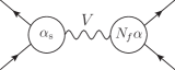
(a) Reducible virtual–virtual contributions within one diagram

  

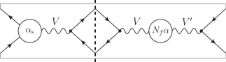
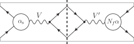
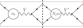
(b) Interference diagrams of type reducible virtual–virtual

Figure 2: Different types of reducible virtual–virtual (vv-red) diagrams contributing at ${\cal O}(N_{f}\alpha_{\mathrm{s}}\alpha)$ to DY-like processes, where the relative orders of the loop corrections are indicated in the vertex blobs.

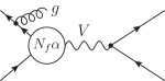
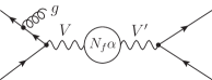
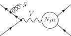
Figure 3: Different types of real–virtual (rv) diagrams contributing at ${\cal O}(N_{f}\alpha_{\mathrm{s}}\alpha)$ to DY-like processes, where the relative orders of the loop corrections are indicated in the vertex blobs.

The vv-red contributions are diagrammatically illustrated in Fig. 2; they combine the closed fermions loops (with either quarks or leptons in the loop) in the EW gauge-boson propagators with the NLO QCD loop diagrams in all possible ways. The rv contributions similarly combine the closed fermions loops in the EW gauge-boson propagators with the real NLO QCD corrections. Figure 3 shows some of the corresponding diagrams for the gluon-emission channel, while their crossed counterparts from $q{\mathrm{g}}$ scattering are not depicted explicitly. Note that at ${\cal O}(N_{f}\alpha_{\mathrm{s}}\alpha)$ there are no rr corrections with double real emission. Such contributions arise from ${\mathrm{g}}\to q\bar{q}$ and $\gamma/{\mathrm{Z}}\to f\bar{f}$ splittings at ${\cal O}(N_{f}\alpha_{\mathrm{s}}^{2})$ and ${\cal O}(N_{f}\alpha^{2})$, respectively, but at ${\cal O}(N_{f}\alpha_{\mathrm{s}}\alpha)$ the corresponding contributions combine a gluon and a photon/Z splitting for a single spinor chain and, thus, vanish due to colour conservation.

In the following we describe in some detail the calculation and results of the two-loop contributions to the self-energies and the corresponding complex renormalization within the complex-mass scheme, which is employed for the gauge-invariant description of the gauge-boson resonances. The evaluation of the matrix elements including those self-energies as well as the evaluation of the reducible vv and rv contributions proceeds fully analogously to the NLO QCD and EW calculations. Since there are no double-unresolved infrared-singular rr contributions, but only infrared singularities of NLO QCD type, we simply employ standard NLO QCD subtraction techniques to combine the vv-red and rv corrections; the vv-1PI corrections do not involve infrared singularities.

In total, we have performed two completely independent calculations, leading to two independent implementations, the results of which are in mutual numerical agreement. The first calculation builds on the Fortran program Rady, which is the basis for the NLO EW and QCD calculations described in Refs. [11, 18, 19]. In order to generalize Rady to the calculation of ${\cal O}(N_{f}\alpha_{\mathrm{s}}\alpha)$ corrections, we just had to dress all ingredients of the NLO QCD calculation with the EW gauge-boson self-energy contributions of ${\cal O}(\alpha)$ and to add the relevant two-loop contributions to the EW gauge-boson self-energy corrections. Infrared singularities are handled with standard QCD dipole subtraction [68]. The graphs and amplitudes for the two-loop self-energies were generated with FeynArts [69, 70] and further algebraically reduced with inhouse Mathematica routines and KIRA [63, 71]. The genuine two-loop corrections of ${\cal O}(N_{f}\alpha_{\mathrm{s}}\alpha)$ contain Goncharov Polylogarithms (GPLs) [72, 73] up to weight three. In the first calculation the numerical evaluation of the necessary GPLs was performed in two steps. In the first step the GPLs were reduced by hand to Harmonic Polylogarithms (HPLs) [74] following the methods introduced in Ref. [75] and in the second step the HPLs were evaluated using the Fortran program CHAPLIN [76]. The second, independent calculation of the corrected cross sections employs antenna subtraction [77] to handle infrared singularities present in the reducible vv-red and rv ${\cal O}(N_{f}\alpha_{\mathrm{s}}\alpha)$ corrections, which were obtained analogously to the first calculation by dressing the NLO QCD calculation with EW gauge-boson self-energies of ${\cal O}(\alpha)$. The two-loop self-energies were generated with QGraf [78] and algebraically reduced to scalar integrals via Matad [79] and FeynCalc [80, 81]. The reduction to master integrals was again performed with KIRA to get the final result in Mathematica. The GPLs contained in the genuine two-loop ${\cal O}(N_{f}\alpha_{\mathrm{s}}\alpha)$ corrections were evaluated using the C++ library GiNaC [82].

2.2 Electroweak gauge-boson self-energies at ${\cal O}(\alpha_{\mathrm{s}}\alpha)$

As explained above, the only 1PI two-loop building blocks required for the ${\cal O}(N_{f}\alpha_{\mathrm{s}}\alpha)$ corrections are the EW gauge-boson self-energies at this order. More precisely, only the transverse parts $\Sigma_{\mathrm{T}}^{V^{\prime}V}(k^{2})$ ($V^{\prime}V=\gamma\gamma,\gamma{\mathrm{Z}},{\mathrm{Z}}{\mathrm{Z}},{\mathrm{W}}{\mathrm{W}}$) of those self-energies are needed, where $k^{2}$ denotes the virtuality of the gauge bosons $V,V^{\prime}$. For the precise relation between the two-point vertex functions $\Gamma^{V^{\prime}V}$ and the self-energies $\Sigma^{V^{\prime}V}$ we follow the conventions of Ref. [45] (identifying $\Sigma^{WW}\equiv\Sigma^{W}$ and defining $M_{A}=0$),

$$\Gamma^{V^{\prime}V}_{\mu\nu}(-k,k)=-g_{\mu\nu}(k^{2}-M^{2}_{V})\delta_{V^{\prime}V}-\left(g_{\mu\nu}-\frac{k_{\mu}k_{\nu}}{k^{2}}\right)\Sigma^{V^{\prime}V}_{{\mathrm{T}}}(k^{2})-\frac{k_{\mu}k_{\nu}}{k^{2}}\Sigma^{V^{\prime}V}_{{\mathrm{L}}}(k^{2}).$$ (2.3)

In the following, only the transverse self-energy parts $\Sigma^{V^{\prime}V}_{{\mathrm{T}}}$ will be considered, because the longitudinal parts $\Sigma^{V^{\prime}V}_{{\mathrm{L}}}$ are not relevant in our calculation. By definition, we do not include tadpole contributions in $\Sigma_{\mathrm{T}}^{V^{\prime}V}$, since tadpoles fully cancel in the considered on-shell renormalization scheme, i.e. our results on $\Sigma_{\mathrm{T}}^{V^{\prime}V}$ correspond to the “parameter-renormalized tadpole scheme” (PRTS) as defined in Refs. [45, 83]. We decompose the ${\cal O}(\alpha_{\mathrm{s}}\alpha)$ contribution $\Sigma_{{\mathrm{T}},(\alpha_{\mathrm{s}}\alpha)}^{V^{\prime}V}(k^{2})$ to the self-energies according to

$$\Sigma_{{\mathrm{T}},(\alpha_{\mathrm{s}}\alpha)}^{V^{\prime}V}(k^{2})=\Sigma_{{\mathrm{T}},(\alpha_{\mathrm{s}}\alpha),\mathrm{1PI}}^{V^{\prime}V}(k^{2})+\Sigma_{{\mathrm{T}},(\alpha_{\mathrm{s}}\alpha),\delta m}^{V^{\prime}V}(k^{2}),$$ (2.4)

where $\Sigma_{{\mathrm{T}},(\alpha_{\mathrm{s}}\alpha),\mathrm{1PI}}^{V^{\prime}V}$ comprises all genuine irreducible two-loop diagrams, as shown in Fig. 4, and $\Sigma_{{\mathrm{T}},(\alpha_{\mathrm{s}}\alpha),\delta m}^{V^{\prime}V}$ represents all fermion loops with insertions of the quark-mass counterterms. In $D=4-2\epsilon$ dimensions, with $\mu$ denoting the arbitrary reference mass scale of dimensional regularization, the mass renormalization constants $\delta m_{q}$ in the on-shell scheme (see Fig. 4) is given by

$$\delta m_{q}=-m_{q}\frac{C_{\mathrm{F}}\alpha_{\mathrm{s}}}{4\pi}\frac{3-2\epsilon}{1-2\epsilon}\bigg{(}\frac{4\pi\mu^{2}}{m_{q}^{2}}\bigg{)}^{\epsilon}\frac{\Gamma(1+\epsilon)}{\epsilon},$$ (2.5)

where $C_{\mathrm{F}}=\frac{4}{3}$ denotes the quadratic Casimir factor of the fundamental representation of $SU(3)$.

= + +
= +

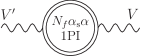
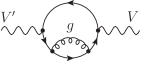
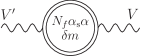
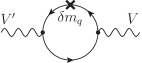
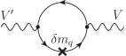
Figure 4: Diagrams contributing to the EW gauge-boson self-energies at ${\cal O}(N_{f}\alpha_{\mathrm{s}}\alpha)$, which all involve closed quark loops. In the first line the contributions to $\Sigma_{{\mathrm{T}},\mathrm{1PI}}^{V^{\prime}V}$ and in the second line the contributions to $\Sigma_{{\mathrm{T}},\delta m}^{V^{\prime}V}$ are shown.

Note that no other one-loop counterterm insertions in one-loop diagrams are relevant at ${\cal O}(N_{f}\alpha_{\mathrm{s}}\alpha)$, because the only other potentially relevant renormalization constants of ${\cal O}(\alpha_{\mathrm{s}})$ are the quark-field renormalization constants, but their contributions to $\Sigma_{{\mathrm{T}},(\alpha_{\mathrm{s}}\alpha)}^{V^{\prime}V}$ fully cancel.

The gauge-boson self-energies are first expressed in terms of the two-loop two-point integrals

$$S_{abcde}(p^{2},m_{1}^{2},m_{2}^{2})={} \left(\frac{(2\pi\mu)^{2\epsilon}}{{\mathrm{i}}\pi^{2}}\right)^{2}\int{\mathrm{d}}^{D}q_{1}\int{\mathrm{d}}^{D}q_{2}\,\frac{1}{(q_{1}^{2})^{a}\,(q_{2}^{2}-m_{1}^{2})^{b}}$$

$${}\times\frac{1}{[(q_{2}+p)^{2}-m_{2}^{2}]^{c}\,[(q_{1}+q_{2})^{2}-m_{1}^{2}]^{d}\,[(q_{1}+q_{2}+p)^{2}-m_{2}^{2}]^{e}},$$ (2.6)

where a graphical representation of these integrals is shown in Fig. 5.

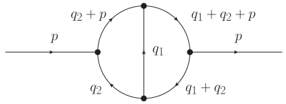
Figure 5: Two-loop sunset topology, corresponding to the self-energy integral $S_{abcde}$ defined in Eq. (2.6).

The prefactor in this definition is chosen in such a way that reducible integrals decompose into the product of the standard one-loop integrals defined in Refs. [83, 45]. The integral functions $S_{abcde}$ obey some obvious symmetries, which are exploited in the formulas below,

$$S_{abcde}(p^{2},m_{1}^{2},m_{2}^{2})={} S_{adebc}(p^{2},m_{1}^{2},m_{2}^{2})=S_{acbed}(p^{2},m_{2}^{2},m_{1}^{2})=S_{aedcb}(p^{2},m_{2}^{2},m_{1}^{2}).$$ (2.7)

Using Laporta’s algorithm [62] as implemented in the program KIRA [63, 71], we reduce the occurring two-loop integrals in terms of the minimal set of master integrals illustrated in Fig. 6.

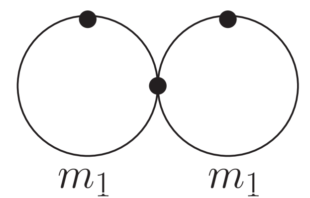
$S_{02020}$

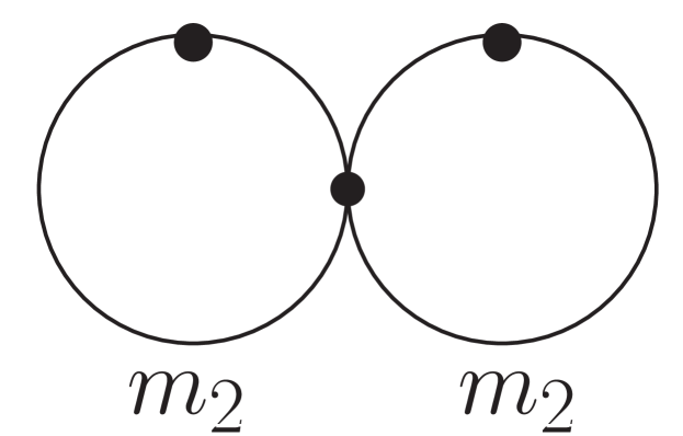
$S_{00202}$

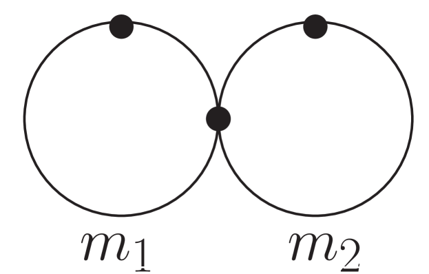
$S_{00220}$

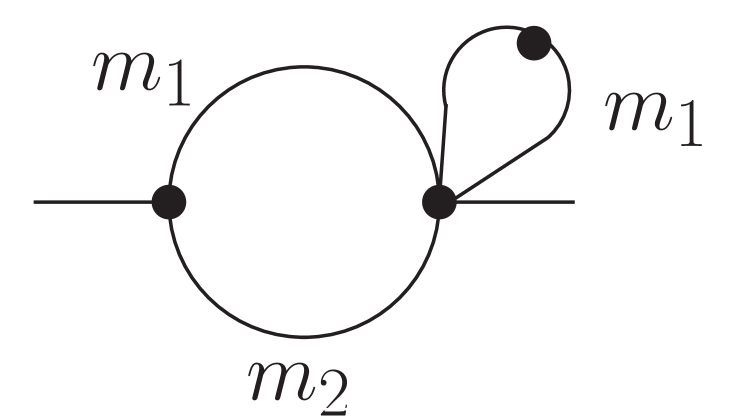
$S_{01120}$

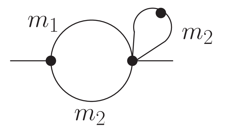
$S_{01102}$

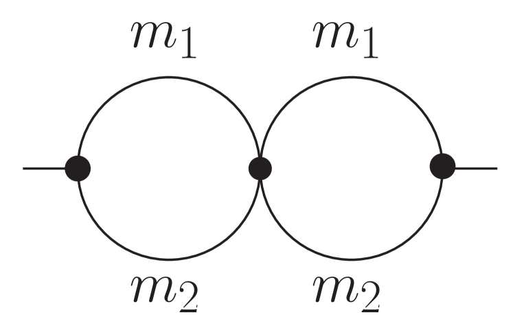
$S_{01111}$

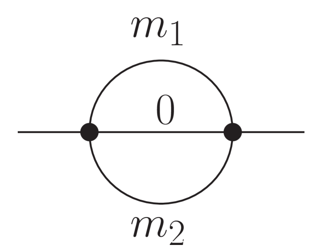
$S_{10110}$

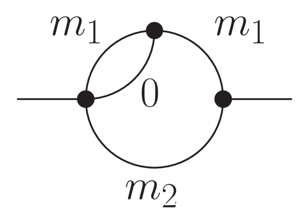
$S_{11110}$

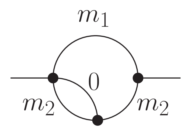
$S_{11101}$

Figure 6: Set of master integrals $S_{abcde}(p^{2},m_{1}^{2},m_{2}^{2})$ for $m_{1}\neq m_{2}$. Dotted lines represent a squared propagator.

For the transverse parts of the self-energies of the neutral EW gauge bosons we explicitly get

$$\Sigma_{{\mathrm{T}},(\alpha_{\mathrm{s}}\alpha),\mathrm{1PI}}^{AA}(s)={} \frac{\alpha_{\mathrm{s}}\alpha}{\pi^{2}}\frac{N_{\mathrm{c}}^{2}-1}{2}\sum_{q}Q_{q}^{2}\,s\,f_{1}(s,m_{q}^{2}),$$ (2.8)

$$\Sigma_{{\mathrm{T}},(\alpha_{\mathrm{s}}\alpha),\mathrm{1PI}}^{AZ}(s)={} \frac{\alpha_{\mathrm{s}}\alpha}{\pi^{2}}\frac{N_{\mathrm{c}}^{2}-1}{2}\sum_{q}(-Q_{q})v_{q}\,s\,f_{1}(s,m_{q}^{2}),$$ (2.9)

$$\Sigma_{{\mathrm{T}},(\alpha_{\mathrm{s}}\alpha),\mathrm{1PI}}^{ZZ}(s)={} \frac{\alpha_{\mathrm{s}}\alpha}{\pi^{2}}\frac{N_{\mathrm{c}}^{2}-1}{2}\sum_{q}\big{[}(v_{q}^{2}+a_{q}^{2})\,s\,f_{1}(s,m_{q}^{2})+a_{q}^{2}\,m_{q}^{2}\,f_{2}(s,m_{q}^{2})\big{]},$$ (2.10)

$$\Sigma_{{\mathrm{T}},(\alpha_{\mathrm{s}}\alpha),\delta m}^{AA}(s)={} \frac{\alpha_{\mathrm{s}}\alpha}{\pi^{2}}\frac{N_{\mathrm{c}}^{2}-1}{2}\sum_{q}Q_{q}^{2}\,m_{q}^{2}\,f_{3}(s,m_{q}^{2}),$$ (2.11)

$$\Sigma_{{\mathrm{T}},(\alpha_{\mathrm{s}}\alpha),\delta m}^{AZ}(s)={} \frac{\alpha_{\mathrm{s}}\alpha}{\pi^{2}}\frac{N_{\mathrm{c}}^{2}-1}{2}\sum_{q}(-Q_{q})v_{q}\,m_{q}^{2}\,f_{3}(s,m_{q}^{2}),$$ (2.12)

$$\Sigma_{{\mathrm{T}},(\alpha_{\mathrm{s}}\alpha),\delta m}^{ZZ}(s)={} \frac{\alpha_{\mathrm{s}}\alpha}{\pi^{2}}\frac{N_{\mathrm{c}}^{2}-1}{2}\sum_{q}m_{q}^{2}\big{[}(v_{q}^{2}+a_{q}^{2})\,f_{3}(s,m_{q}^{2})+a_{q}^{2}\,f_{4}(s,m_{q}^{2})\big{]},$$ (2.13)

where $(N_{\mathrm{c}}^{2}-1)/2=N_{\mathrm{c}}C_{\mathrm{F}}=4$ originates from the SU($N_{\mathrm{c}}$) colour algebra with $N_{\mathrm{c}}=3$. The sums $\sum_{q}$ extend over all quark flavours $q\in\{{\mathrm{u}},{\mathrm{d}},{\mathrm{c}},{\mathrm{s}},{\mathrm{t}},{\mathrm{b}}\}$ with relative electric charges $Q_{q}$ and third components $I^{3}_{{\mathrm{w}},q}=\pm\frac{1}{2}$ of the weak isospin, and the vector and axial-vector couplings of quark $q$ to the Z boson are denoted as

$$v_{q}=\frac{I^{3}_{{\mathrm{w}},q}-2s_{\mathrm{w}}^{2}Q_{q}}{2s_{\mathrm{w}}c_{\mathrm{w}}},\qquad a_{q}=\frac{I^{3}_{{\mathrm{w}},q}}{2s_{\mathrm{w}}c_{\mathrm{w}}}.$$ (2.14)

Keeping the full dependence on $D=4-2\epsilon$ in order to facilitate the later specialization to specific mass patterns, the auxiliary functions $f_{k}$ $(k=1,\dots,4)$ are given by

$$f_{1}(s,m^{2})={} \frac{1-\epsilon}{2s}\,S_{10110}+\frac{1-\epsilon}{2(3-2\epsilon)\epsilon}\left[2-3\epsilon+2\epsilon^{2}+4(1-\epsilon)(1+2\epsilon)\frac{m^{2}}{s}\right]S_{11110}$$

$${}+\frac{1}{4\epsilon}\left[-\frac{(1-\epsilon)(2-\epsilon+2\epsilon^{2})}{3-2\epsilon}-\frac{2m^{2}}{(3-2\epsilon)s}+\frac{2(1-2\epsilon)m^{2}}{4m^{2}-s}\right]S_{01111}$$

$${}+\frac{m^{2}}{\epsilon s}\left[\frac{2-6\epsilon+7\epsilon^{2}-2\epsilon^{3}}{3-2\epsilon}-\frac{2(2-3\epsilon+2\epsilon^{2})m^{2}}{4m^{2}-s}\right]S_{01120}$$

$${}+\frac{m^{2}}{2\epsilon s}\left[-\frac{2-3\epsilon+2\epsilon^{2}}{(1-2\epsilon)(3-2\epsilon)}+\frac{4(1-\epsilon)m^{2}}{4m^{2}-s}\right]S_{02020},$$ (2.15)

$$f_{2}(s,m^{2})={} \frac{(1-2\epsilon)}{(3-2\epsilon)s}\,S_{10110}+\frac{1}{3-2\epsilon}\left[-\frac{6-9\epsilon+2\epsilon^{2}}{\epsilon}+\frac{4(1-2\epsilon)m^{2}}{s}\right]S_{11110}$$

$${}+\frac{1}{\epsilon}\left[\frac{(1-\epsilon)(3-3\epsilon+2\epsilon^{2})}{3-2\epsilon}-\frac{2(1-2\epsilon)m^{2}}{4m^{2}-s}\right]S_{01111}$$

$${}-2m^{2}\left[\frac{2}{(3-2\epsilon)s}-\frac{2-3\epsilon+2\epsilon^{2}}{\epsilon(4m^{2}-s)}\right]S_{01120}$$

$${}+m^{2}\left[\frac{1}{(3-2\epsilon)(1-\epsilon)s}-\frac{2(1-\epsilon)}{\epsilon(4m^{2}-s)}\right]S_{02020},$$ (2.16)

$$f_{3}(s,m^{2})={} -(3-2\epsilon)\left[\frac{\epsilon}{1-2\epsilon}+\frac{2m^{2}}{4m^{2}-s}\right]S_{01120}+\frac{2(3-2\epsilon)m^{2}}{(1-2\epsilon)(4m^{2}-s)}S_{02020},$$ (2.17)

$$f_{4}(s,m^{2})={} (3-2\epsilon)\left[\frac{1}{1-2\epsilon}+\frac{2m^{2}}{4m^{2}-s}\right]S_{01120}-\frac{2(3-2\epsilon)m^{2}}{(1-2\epsilon)(4m^{2}-s)}\,S_{02020},$$ (2.18)

with suppressed arguments of the integral functions $S_{abcde}(s,m^{2},m^{2})$. The ${\cal O}(\alpha_{\mathrm{s}}\alpha)$ contributions to the transverse part of the W-boson self-energy is given by

$$\Sigma_{{\mathrm{T}},(\alpha_{\mathrm{s}}\alpha),\mathrm{1PI}}^{W}(s)={} \frac{\alpha_{\mathrm{s}}\alpha}{2\pi^{2}s_{\mathrm{w}}^{2}}\frac{N_{\mathrm{c}}^{2}-1}{2}\sum_{j=1}^{3}\left[sf_{5}(s,m_{d_{j}}^{2},m_{u_{j}}^{2})+(m_{d_{j}}\leftrightarrow m_{u_{j}})\right],$$ (2.19)

$$\Sigma_{{\mathrm{T}},(\alpha_{\mathrm{s}}\alpha),\delta m}^{W}(s)={} \frac{\alpha_{\mathrm{s}}\alpha}{2\pi^{2}s_{\mathrm{w}}^{2}}\frac{N_{\mathrm{c}}^{2}-1}{2}\sum_{j=1}^{3}\left[m_{u_{j}}^{2}f_{6}(s,m_{d_{j}}^{2},m_{u_{j}}^{2})+(m_{d_{j}}\leftrightarrow m_{u_{j}})\right],$$ (2.20)

where the sums $\sum_{j}$ extend over the three generations of up-type and down-type quarks $u_{j}$ and $d_{j}$, respectively. The auxiliary function $f_{k}$ $(k=5,6)$ are given by

$$f_{5}(s,m_{1}^{2},m_{2}^{2})={} \left[1-\epsilon+\frac{(1-2\epsilon)(m_{1}^{2}+m_{2}^{2})}{2(3-2\epsilon)s}\right]\frac{S_{10110}}{8s}$$

$${}+\frac{1}{16(3-2\epsilon)\epsilon}\biggl{[}(2-3\epsilon+2\epsilon^{2})\left(2(1-\epsilon)-(1-2\epsilon)\frac{m_{1}^{2}}{s}-\frac{m_{1}^{4}}{s^{2}}\right)$$

$$\qquad{}-(2-3\epsilon)(1-2\epsilon)^{2}\frac{m_{2}^{2}}{s}+4(1-2\epsilon^{2})\frac{m_{1}^{2}m_{2}^{2}}{s^{2}}-(2-5\epsilon+6\epsilon^{2})\frac{m_{2}^{4}}{s^{2}}\biggr{]}S_{11101}$$

$${}-\frac{1}{16\epsilon}\left[\frac{(1-\epsilon)(2-\epsilon+2\epsilon^{2})}{3-2\epsilon}+\frac{(1-2\epsilon)(1-\epsilon^{2})}{3-2\epsilon}\frac{m_{1}^{2}+m_{2}^{2}}{s}\right.$$

$$\qquad\left.{}+4(1-2\epsilon)\frac{m_{1}^{2}m_{2}^{2}}{\lambda}\right]S_{01111}$$

$${}+\frac{m_{2}^{2}}{8\epsilon s}\left[\frac{2(2-6\epsilon+7\epsilon^{2}-2\epsilon^{3})}{3-2\epsilon}-\frac{(2-3\epsilon+2\epsilon^{2})m_{1}^{2}}{(3-2\epsilon)s}+\frac{(2-7\epsilon+2\epsilon^{2})m_{2}^{2}}{(3-2\epsilon)s}\right.$$

$$\qquad\left.{}-\frac{2(2-3\epsilon+2\epsilon^{2})m_{1}^{2}(m_{1}^{2}-m_{2}^{2}-s)}{\lambda}\right]S_{01102}$$

$${}+\frac{m_{1}^{2}m_{2}^{2}}{8\epsilon s^{2}}\left[\frac{(1-2\epsilon)(2-\epsilon)}{(3-2\epsilon)(1-\epsilon)}+\frac{2(1-\epsilon)s(m_{1}^{2}+m_{2}^{2}-s)}{\lambda}\right]S_{00220}$$

$${}-\frac{m_{2}^{2}}{16\epsilon s}\left[\frac{(2-17\epsilon+26\epsilon^{2}-8\epsilon^{3})m_{2}^{2}+(2-3\epsilon+2\epsilon^{2})(m_{1}^{2}+2(1-\epsilon)s)}{(1-2\epsilon)(3-2\epsilon)(1-\epsilon)s}\right.$$

$$\qquad\left.{}+\frac{8(1-\epsilon)m_{1}^{2}m_{2}^{2}}{\lambda}\right]S_{00202},$$ (2.21)

$$f_{6}(s,m_{1}^{2},m_{2}^{2})={} \frac{3-2\epsilon}{4}\biggl{\{}\left[\frac{(1-2\epsilon)s-m_{1}^{2}+m_{2}^{2}}{2(1-2\epsilon)s}+\frac{m_{1}^{2}(s-m_{1}^{2}+m_{2}^{2})}{\lambda}\right]S_{01102}$$

$$\qquad{}+\frac{m_{1}^{2}}{1-2\epsilon}\left[\frac{1}{2(1-\epsilon)s}+\frac{m_{1}^{2}+m_{2}^{2}-s}{\lambda}\right]S_{00220}$$

$$\qquad{}-\frac{m_{2}^{2}}{1-2\epsilon}\left[\frac{1}{2(1-\epsilon)s}+\frac{2m_{1}^{2}}{\lambda}\right]S_{00202}\biggr{\}}$$ (2.22)

with the Källen function

$$\lambda=(s-m_{1}^{2}-m_{2}^{2})^{2}-4m_{1}^{2}m_{2}^{2}$$ (2.23)

and the arguments of the integral functions given by $S_{abcde}(s,m_{1}^{2},m_{2}^{2})$. Note that the interchange $(m_{d_{j}}\leftrightarrow m_{u_{j}})$ of the up- and down-type quark masses in (2.19) and (2.20) also concerns the arguments of the integral functions; this change of arguments can, however, be achieved by rearranging labels in $S_{abcde}$ using (2.7).

For massless fermions, only the functions $f_{1}$ and $f_{5}$ are relevant and given by

$$f_{1}(s,0)=4f_{5}(s,0,0)=\left(\frac{4\pi\mu^{2}}{-s-{\mathrm{i}}0}\right)^{2\epsilon}\Gamma(1+\epsilon)^{2}\left[\frac{1}{8\epsilon}+\frac{55}{48}-\zeta_{3}+{\cal O}(\epsilon)\right]$$ (2.24)

to the relevant order in $\epsilon$.

In addition to the self-energies $\Sigma_{{\mathrm{T}}}^{V^{\prime}V}(s)$ for non-vanishing $s$, we in particular need the W-boson self-energy at zero-momentum transfer in the application of the $G_{\mu}$ input-parameter scheme below. In this limit the two-mass two-loop tadpole integrals $T_{abc}$, defined by

$$T_{abc}(m_{1}^{2},m_{2}^{2})={} \left(\frac{(2\pi\mu)^{2\epsilon}}{{\mathrm{i}}\pi^{2}}\right)^{2}\int{\mathrm{d}}^{D}q_{1}\int{\mathrm{d}}^{D}q_{2}\,\frac{1}{(q_{1}^{2})^{a}\,(q_{2}^{2}-m_{1}^{2})^{b}[(q_{1}+q_{2})^{2}-m_{2}^{2}]^{c}},$$ (2.25)

are needed in addition. They obey the following symmetry relations

$$T_{abc}(m_{1}^{2},m_{2}^{2})=T_{acb}(m_{2}^{2},m_{1}^{2}).$$ (2.26)

Since the numerical evaluation of $\Sigma_{{\mathrm{T}},(\alpha_{\mathrm{s}}\alpha)}^{W}(0)$ is somewhat non-trivial in the above representation, we here give an explicit form for $\Sigma_{{\mathrm{T}},(\alpha_{\mathrm{s}}\alpha)}^{W}(0)$ suitable for a numerical evaluation, which was obtained by explicitly expanding the master integrals about $s=0$ with the help of the differential equations used to calculate them (see App. A),

$$\Sigma_{{\mathrm{T}},(\alpha_{\mathrm{s}}\alpha),\mathrm{1PI}}^{W}(0)={} \frac{\alpha_{\mathrm{s}}\alpha}{2\pi^{2}s_{\mathrm{w}}^{2}}\frac{N_{\mathrm{c}}^{2}-1}{2}\sum_{j=1}^{3}\,\Big{[}f_{7}(m_{d_{j}}^{2},m_{u_{j}}^{2})+(m_{d_{j}}\leftrightarrow m_{u_{j}})\Big{]},$$ (2.27)

$$\Sigma_{{\mathrm{T}},(\alpha_{\mathrm{s}}\alpha),\delta m}^{W}(0)={} \frac{\alpha_{\mathrm{s}}\alpha}{2\pi^{2}s_{\mathrm{w}}^{2}}\frac{N_{\mathrm{c}}^{2}-1}{2}\sum_{j=1}^{3}\left[m_{u_{j}}^{2}f_{8}(m_{d_{j}}^{2},m_{u_{j}}^{2})+(m_{d_{j}}\leftrightarrow m_{u_{j}})\right].$$ (2.28)

The auxiliary functions $f_{k}$ ($k=7,8$) are given by

$$f_{7}(m_{1}^{2},m_{2}^{2})={} \frac{m_{2}^{4}}{4(2-\epsilon)}\left[\frac{m_{2}^{2}}{(1-\epsilon)\lambda_{0}}+\frac{(3-2\epsilon)(1-\epsilon)}{(1-2\epsilon)(m_{1}^{2}-m_{2}^{2})}\right]S_{00202}$$

$${}-\frac{m_{1}^{2}m_{2}^{4}}{4(2-\epsilon)(1-\epsilon)\lambda_{0}}S_{00220}+\frac{1-\epsilon}{8(2-\epsilon)}T_{111}(m_{1}^{2},m_{2}^{2}),$$ (2.29)

$$f_{8}(m_{1}^{2},m_{2}^{2})={} \frac{(3-2\epsilon)m_{2}^{2}}{4(2-\epsilon)(1-2\epsilon)\lambda_{0}}\Bigl{\{}\Bigl{[}(1-\epsilon)m_{2}^{2}-(2-\epsilon)m_{1}^{2}\Bigr{]}S_{00202}+m_{1}^{2}\,S_{00220}\Bigr{\}},$$ (2.30)

where $\lambda_{0}$ is obtained by evaluating $\lambda$ in (2.23) at $s=0$,

$$\lambda_{0}=(m_{1}^{2}-m_{2}^{2})^{2},$$ (2.31)

and the integrals $S_{abcde}$ have the arguments $S_{abcde}(0,m_{1}^{2},m_{2}^{2})$. Note that the appearing master integrals $S_{02020}$ and $S_{00202}$ are actually products of one-loop tadpole integrals and can be expressed in terms of $T_{abc}$ via

$$S_{00202}(s,m_{1}^{2},m_{2}^{2})={} S_{00202}(0,m_{1}^{2},m_{2}^{2})=T_{022}(m_{2}^{2},m_{2}^{2}),$$

$$S_{00220}(s,m_{1}^{2},m_{2}^{2})={} S_{00220}(0,m_{1}^{2},m_{2}^{2})=T_{022}(m_{1}^{2},m_{2}^{2}).$$ (2.32)

The limits of the functions $f_{k}(m_{1}^{2},m_{2}^{2})$ ($k=7,8$) in which one of the two quark masses vanishes can be obtained by simply evaluating (2.29) and (2.30) with the corresponding mass set to zero. In the case in which both quark masses are zero the whole contribution of the corresponding massless quark generations to $\Sigma_{{\mathrm{T}},(\alpha_{\mathrm{s}}\alpha)}^{W}(0)$ vanishes because of dimensional reasons.

The ${\cal O}(N_{f}\alpha_{s}\alpha)$ corrections to the EW gauge-boson self-energies have been calculated some time ago in Refs. [56, 57, 58, 59, 60, 61]. We have compared our results with the ones given in Ref. [56] and find full analytical agreement in the case of vanishing quark masses. For non-vanishing quark masses we find numerical agreement for $\Sigma_{{\mathrm{T}},(\alpha_{\mathrm{s}}\alpha)}^{V^{\prime}V}(k^{2})$ with those results.

2.3 Renormalization and complex-mass scheme

In our calculation of ${\cal O}(N_{f}\alpha_{\mathrm{s}}\alpha)$ corrections we employ straightforward generalizations of the on-shell renormalization schemes and their complexified versions used in the NLO EW calculations for DY-like processes described in Refs. [11, 18, 19]. At NLO the real formulations and their complex generalizations are described in Refs. [83, 45] and Refs. [66, 45], respectively.

Since the reducible vv and rv contributions only involve one-loop subdiagrams, their calculation does not require any generalization beyond NLO. The only generalization to NNLO concerns the calculation of the counterterms required in the gauge-boson two-point functions and in the gauge-boson–fermion vertices for the EW gauge bosons. However, owing to our restriction to the $N_{f}$-enhanced ${\cal O}(\alpha_{\mathrm{s}}\alpha)$ corrections, all relevant contributions to the needed counterterms originate from the contributions to the EW gauge-boson self-energies $\Sigma_{\mathrm{T}}^{V^{\prime}V}$ considered above. In detail, we need the ${\cal O}(N_{f}\alpha_{\mathrm{s}}\alpha)$ contributions to the following renormalization constants in the complex-mass scheme [66, 45]: the gauge-boson mass renormalization constants $\delta\mu_{\mathrm{W}}^{2}$, $\delta\mu_{\mathrm{Z}}^{2}$, the gauge-boson field renormalization constants $\delta{\cal Z}_{V^{\prime}V}$, the renormalization constants $\delta c_{\mathrm{w}}$ for the weak mixing angle, and the charge renormalization constant $\delta Z_{e}$.

The W- and Z-boson mass parameters $\mu_{V}^{2}$ ($V={\mathrm{W}},{\mathrm{Z}}$) are defined as the locations of the poles in the complex $k^{2}$ plane of the W/Z propagators and are decomposed into real and imaginary parts according to

$$\mu_{V}^{2}=M_{V}^{2}-{\mathrm{i}}M_{V}\Gamma_{V},\qquad V={\mathrm{W}},{\mathrm{Z}},$$ (2.33)

where the real mass and width parameters $M_{V}$ and $\Gamma_{V}$ deviate from their counterparts $M_{V,\mathrm{OS}}$ and $\Gamma_{V,\mathrm{OS}}$ in the real on-shell (OS) scheme at the two-loop level. In good approximation, the connection is [45]

$$M_{V}=\frac{M_{V,\mathrm{OS}}}{\sqrt{1+\Gamma_{V,\mathrm{OS}}^{2}/M_{V,\mathrm{OS}}^{2}}},\qquad\Gamma_{V}=\frac{\Gamma_{V,\mathrm{OS}}}{\sqrt{1+\Gamma_{V,\mathrm{OS}}^{2}/M_{V,\mathrm{OS}}^{2}}}.$$ (2.34)

Since the on-shell mass and field renormalization of the EW gauge bosons is simply based on some momentum subtraction for the vertex two-point function, the perturbative contributions to the renormalization constants $\delta\mu_{V}^{2}$ and $\delta{\cal Z}_{V^{\prime}V}$ are in one-to-one correspondence with the corresponding orders in the required self-energies $\Sigma_{\mathrm{T}}^{V^{\prime}V}$. Denoting again the order of the contributions by some subscript “($\alpha_{\mathrm{s}}\alpha$)” for ${\cal O}(\alpha_{\mathrm{s}}\alpha)$, we therefore get

$$\delta\mu^{2}_{{\mathrm{W}},(\alpha_{\mathrm{s}}\alpha)} {}=\Sigma^{W}_{{\mathrm{T}},(\alpha_{\mathrm{s}}\alpha)}(\mu^{2}_{\mathrm{W}}),\qquad \delta\mu^{2}_{{\mathrm{Z}},(\alpha_{\mathrm{s}}\alpha)} {}=\Sigma^{ZZ}_{{\mathrm{T}},(\alpha_{\mathrm{s}}\alpha)}(\mu^{2}_{\mathrm{Z}}),$$ (2.35)

$$\delta\mathcal{Z}_{W,(\alpha_{\mathrm{s}}\alpha)} {}=-\Sigma^{\prime W}_{{\mathrm{T}},(\alpha_{\mathrm{s}}\alpha)}(\mu^{2}_{\mathrm{W}}),$$

$$\delta\mathcal{Z}_{ZA,(\alpha_{\mathrm{s}}\alpha)} {}=\frac{2}{\mu^{2}_{\mathrm{Z}}}\Sigma^{AZ}_{{\mathrm{T}},(\alpha_{\mathrm{s}}\alpha)}(0),\qquad \delta\mathcal{Z}_{AZ,(\alpha_{\mathrm{s}}\alpha)} {}=-\frac{2}{\mu^{2}_{\mathrm{Z}}}\Sigma^{AZ}_{{\mathrm{T}},(\alpha_{\mathrm{s}}\alpha)}(\mu^{2}_{\mathrm{Z}}),\qquad$$

$$\delta\mathcal{Z}_{ZZ,(\alpha_{\mathrm{s}}\alpha)} {}=-\Sigma^{\prime ZZ}_{{\mathrm{T}},(\alpha_{\mathrm{s}}\alpha)}(\mu^{2}_{\mathrm{Z}}),\qquad \delta\mathcal{Z}_{AA,(\alpha_{\mathrm{s}}\alpha)} {}=-\Sigma^{\prime AA}_{{\mathrm{T}},(\alpha_{\mathrm{s}}\alpha)}(0),$$ (2.36)

where $\Sigma^{\prime V^{\prime}V}(k^{2})\equiv(\partial\Sigma^{V^{\prime}V}/\partial k^{2})(k^{2})$. In quantities, in which the distinction between ${\cal O}(N_{f}\alpha_{\mathrm{s}}\alpha)$ and ${\cal O}(\alpha_{\mathrm{s}}\alpha)$ is not necessary, we simply write $(\alpha_{\mathrm{s}}\alpha)$ as subscript.

In order to avoid the evaluation of self-energies with complex $k^{2}$, we follow the “simplified version” of the complex-mass scheme based on Taylor expanding $\Sigma^{\prime V^{\prime}V}(\mu_{V}^{2})$ about the real part $M_{V}^{2}$ of $\mu_{V}^{2}$ up to the relevant order. This leads to

$$\delta\mu^{2}_{{\mathrm{W}},(\alpha_{\mathrm{s}}\alpha)} {}={}\hbox to0.0pt{$\Sigma^{W}_{{\mathrm{T}},(\alpha_{\mathrm{s}}\alpha)}(M_{\mathrm{W}}^{2})+(\mu^{2}_{\mathrm{W}}-M_{\mathrm{W}}^{2})\Sigma^{\prime W}_{{\mathrm{T}},(\alpha_{\mathrm{s}}\alpha)}(M_{\mathrm{W}}^{2})$,\hss}$$

$$\delta\mu^{2}_{{\mathrm{Z}},(\alpha_{\mathrm{s}}\alpha)} {}={}\hbox to0.0pt{$\Sigma^{ZZ}_{{\mathrm{T}},(\alpha_{\mathrm{s}}\alpha)}(M_{\mathrm{Z}}^{2})+(\mu^{2}_{\mathrm{Z}}-M_{\mathrm{Z}}^{2})\Sigma^{\prime ZZ}_{{\mathrm{T}},(\alpha_{\mathrm{s}}\alpha)}(M_{\mathrm{Z}}^{2}),$\hss}$$ (2.37)

$$\delta\mathcal{Z}_{W,(\alpha_{\mathrm{s}}\alpha)} {}=-\Sigma^{\prime W}_{{\mathrm{T}},(\alpha_{\mathrm{s}}\alpha)}(M_{\mathrm{W}}^{2}),\qquad\delta\mathcal{Z}_{ZA,(\alpha_{\mathrm{s}}\alpha)}{}=\frac{2}{\mu^{2}_{\mathrm{Z}}}\Sigma^{AZ}_{{\mathrm{T}},(\alpha_{\mathrm{s}}\alpha)}(0),$$

$$\delta\mathcal{Z}_{AZ,(\alpha_{\mathrm{s}}\alpha)} {}=-\frac{2}{M_{\mathrm{Z}}^{2}}\Sigma^{AZ}_{{\mathrm{T}},(\alpha_{\mathrm{s}}\alpha)}(M_{\mathrm{Z}}^{2})+\left(\frac{\mu^{2}_{\mathrm{Z}}}{M_{\mathrm{Z}}^{2}}-1\right)\delta\mathcal{Z}_{ZA,(\alpha_{\mathrm{s}}\alpha)},$$

$$\delta\mathcal{Z}_{ZZ,(\alpha_{\mathrm{s}}\alpha)} {}=-\Sigma^{\prime ZZ}_{{\mathrm{T}},(\alpha_{\mathrm{s}}\alpha)}(M_{\mathrm{Z}}^{2}).$$ (2.38)

Note that some care is required in order to catch all the relevant terms in the evaluation of $\delta\mu_{V}^{2}$ above. Firstly, there is no ${\cal O}(\alpha_{\mathrm{s}})$ contribution to $\Sigma_{\mathrm{T}}^{V^{\prime}V}$ at NLO, and $\Gamma_{V}$ counts as ${\cal O}(\alpha)$, so that no additional terms of ${\cal O}(\alpha_{\mathrm{s}}\alpha)$ arise from higher terms in the Taylor expansion (2.3) of $\Sigma_{\mathrm{T}}^{V^{\prime}V}$ at NLO. Secondly, we do not need to include any extra term like $c_{\mathrm{T}}^{\mathrm{W}}$ as introduced in Refs. [66, 45] that occurs at NLO EW as a consequence that $k^{2}=M_{\mathrm{W}}^{2}$ is rather a branch point than a pole of the W propagator, because this subtlety arises from an infrared singularity in on-shell diagrams with photon exchange of the W boson. However, at ${\cal O}(\alpha_{\mathrm{s}}\alpha)$, the self-energies $\Sigma_{\mathrm{T}}^{V^{\prime}V}$ do not involve infrared singularities, i.e. $\Sigma_{{\mathrm{T}},(\alpha_{\mathrm{s}}\alpha)}^{W}$ is analytic at $k^{2}=\mu^{2}_{\mathrm{W}}$, and no extra terms occur.

The renormalization constants $\delta c_{\mathrm{w}}$ and $\delta s_{\mathrm{w}}$ for the (complex) cosine and sine of the weak mixing angle are fixed by the condition that the identity

$$c_{\mathrm{w}}^{2}=1-s_{\mathrm{w}}^{2}=\frac{\mu^{2}_{{\mathrm{W}}}}{\mu^{2}_{{\mathrm{Z}}}}$$ (2.39)

holds both for bare and renormalized quantities. Again, since $\Sigma_{\mathrm{T}}^{V^{\prime}V}$ does not receive ${\cal O}(\alpha_{\mathrm{s}})$ contributions, we get for the contributions to $\delta c_{\mathrm{w}}$ and $\delta s_{\mathrm{w}}$ at ${\cal O}(\alpha_{\mathrm{s}}\alpha)$

$$\frac{\delta s_{{\mathrm{w}},(\alpha_{\mathrm{s}}\alpha)}}{s_{\mathrm{w}}}=-\frac{c_{\mathrm{w}}^{2}}{s_{\mathrm{w}}^{2}}\frac{\delta c_{{\mathrm{w}},(\alpha_{\mathrm{s}}\alpha)}}{c_{\mathrm{w}}}=-\frac{c_{\mathrm{w}}^{2}}{2s_{\mathrm{w}}^{2}}\left(\frac{\delta\mu^{2}_{{\mathrm{W}},(\alpha_{\mathrm{s}}\alpha)}}{\mu^{2}_{\mathrm{W}}}-\frac{\delta\mu^{2}_{{\mathrm{Z}},(\alpha_{\mathrm{s}}\alpha)}}{\mu^{2}_{\mathrm{Z}}}\right).$$ (2.40)

The determination of the charge renormalization constant $\delta Z_{e}$ beyond NLO deserves some care. It is derived from the condition that the renormalized fermion–photon vertex for on-shell fermions does not receive a correction in the “Thomson limit” of vanishing photon momentum. Using symmetry arguments similar to the arguments based on a Ward identity in quantum electrodynamics (QED), it is possible to express $\delta Z_{e}$ in terms of gauge-boson self-energies instead of vertex-correction formfactors. For the SM this derivation based on Lee identities is spelled out in App. C of Ref. [45] at NLO. Taking the fermion of the renormalization condition in the Thomson limit as a lepton, the only source for ${\cal O}(\alpha_{\mathrm{s}}\alpha)$ contributions in a generalization of this derivation are closed quark loops in the gauge-boson self-energies and related self-energies involving Goldstone bosons. Since those self-energies do not receive ${\cal O}(\alpha_{\mathrm{s}})$ contributions, no reducible ${\cal O}(\alpha_{\mathrm{s}}\alpha)$ corrections occur in the derivation. Therefore, all identities that are given in App. C of Ref. [45] for ${\cal O}(\alpha)$ corrections are valid for ${\cal O}(\alpha_{\mathrm{s}}\alpha)$ as well, with all corrections but the self-energies of the gauge-boson and Goldstone-boson sectors vanishing. The final result for $\delta Z_{e}$ then takes a form fully analogous to NLO,

$$\delta Z_{e,(\alpha_{\mathrm{s}}\alpha)}=\frac{1}{2}\Sigma^{\prime AA}_{{\mathrm{T}},(\alpha_{\mathrm{s}}\alpha)}(0)-\frac{s_{\mathrm{w}}}{c_{\mathrm{w}}}\frac{\Sigma^{AZ}_{{\mathrm{T}},(\alpha_{\mathrm{s}}\alpha)}(0)}{\mu^{2}_{\mathrm{Z}}}.$$ (2.41)

Specifically to ${\cal O}(\alpha_{\mathrm{s}}\alpha)$ this result simplifies to

$$\delta Z_{e,(\alpha_{\mathrm{s}}\alpha)}=\frac{1}{2}\Sigma^{\prime AA}_{{\mathrm{T}},(\alpha_{\mathrm{s}}\alpha)}(0),$$ (2.42)

because

$$\Sigma^{AZ}_{{\mathrm{T}},(\alpha_{\mathrm{s}}\alpha)}(k^{2})\equiv 0,$$ (2.43)

which holds as a consequence of Slavnov–Taylor (ST) identities.

The same result can be obtained more directly within the background-field method (BFM) [84, 85, 86, 87, 88], which is applied to the SM in Refs. [89, 45]. Owing to the gauge invariance of the background-field effective action, the Ward identities for the fermion–photon vertex takes the same simple form as in QED to all perturbative orders. In particular, Eq. (2.42) holds within the BFM to all orders. Consequently, the QED-like result (2.42) for $\delta Z_{e}$ trivially carries over to the SM in its BFM formulation in each perturbative order. We note in passing that we have checked explicitly all ST identities for the ${\cal O}(\alpha_{\mathrm{s}}\alpha)$ contributions to the EW gauge-boson two-point functions $\Gamma^{V^{\prime}V}$ considered in the previous section. At ${\cal O}(\alpha_{\mathrm{s}}\alpha)$ these ST identities are formally identical to the BFM Ward identities given in Eqs. (59)–(61) in Ref. [45].

The renormalization constants defined above enter the amplitudes for the ${\cal O}(N_{f}\alpha_{\mathrm{s}}\alpha)$ corrections in two different ways. On the one hand, they are part of the renormalized gauge-boson self-energies $\Sigma_{{\mathrm{R}},{\mathrm{T}}}^{V^{\prime}V}$,

$$\Sigma^{V^{\prime}V}_{{\mathrm{R}},{\mathrm{T}},(\alpha_{\mathrm{s}}\alpha)}(k^{2})={} \Sigma^{V^{\prime}V}_{{\mathrm{T}},(\alpha_{\mathrm{s}}\alpha)}(k^{2})+\frac{1}{2}(k^{2}-\mu_{V}^{2})\delta{\cal Z}_{VV^{\prime},(\alpha_{\mathrm{s}}\alpha)}+\frac{1}{2}(k^{2}-\mu_{V^{\prime}}^{2})\delta{\cal Z}_{V^{\prime}V,(\alpha_{\mathrm{s}}\alpha)}$$

$${}-\delta_{V^{\prime}V}\delta\mu_{V,(\alpha_{\mathrm{s}}\alpha)}^{2},$$ (2.44)

where we set $\mu_{A}=0$. On the other hand, they enter the gauge-boson–fermion counterterms, where they change the LO coupling factors $g_{V\bar{f}f^{\prime}}^{\sigma}$ with chirality $\sigma=\pm$ by the factors

$$\delta^{\mathrm{ct},\sigma}_{W\bar{f}f^{\prime},(\alpha_{\mathrm{s}}\alpha)}={} \delta Z_{e,(\alpha_{\mathrm{s}}\alpha)}-\frac{\delta s_{{\mathrm{w}},(\alpha_{\mathrm{s}}\alpha)}}{s_{\mathrm{w}}}+\frac{1}{2}\delta{\cal Z}_{W,(\alpha_{\mathrm{s}}\alpha)},$$ (2.45)

$$\delta^{\mathrm{ct},\sigma}_{Z\bar{f}f,(\alpha_{\mathrm{s}}\alpha)}={} \frac{\delta g_{Z\bar{f}f,(\alpha_{\mathrm{s}}\alpha)}^{\sigma}}{g_{Z\bar{f}f}^{\sigma}}+\frac{1}{2}\delta{\cal Z}_{ZZ,(\alpha_{\mathrm{s}}\alpha)}-\frac{Q_{f}}{2g_{Z\bar{f}f}^{\sigma}}\delta{\cal Z}_{AZ,(\alpha_{\mathrm{s}}\alpha)},$$ (2.46)

$$\delta^{\mathrm{ct},\sigma}_{A\bar{f}f,(\alpha_{\mathrm{s}}\alpha)}={} \delta Z_{e,(\alpha_{\mathrm{s}}\alpha)}+\frac{1}{2}\delta{\cal Z}_{AA,(\alpha_{\mathrm{s}}\alpha)}-\frac{g_{Z\bar{f}f}^{\sigma}}{2Q_{f}}\delta{\cal Z}_{ZA,(\alpha_{\mathrm{s}}\alpha)},$$ (2.47)

where

$$g_{Z\bar{f}f}^{\sigma}={} -\frac{s_{\mathrm{w}}}{c_{\mathrm{w}}}Q_{f}+\frac{I_{{\mathrm{w}},f}^{3}}{s_{\mathrm{w}}c_{\mathrm{w}}}\,\delta_{\sigma-},\qquad g_{A\bar{f}f}^{\sigma}=-Q_{f},$$ (2.48)

$$\delta g_{Z\bar{f}f}^{\sigma}={} g_{Z\bar{f}f}^{\sigma}\left(\delta Z_{e,(\alpha_{\mathrm{s}}\alpha)}+\frac{1}{c_{\mathrm{w}}^{2}}\frac{\delta s_{{\mathrm{w}},(\alpha_{\mathrm{s}}\alpha)}}{s_{\mathrm{w}}}\right)-\frac{2I_{{\mathrm{w}},f}^{3}}{s_{\mathrm{w}}c_{\mathrm{w}}}\frac{\delta s_{{\mathrm{w}},(\alpha_{\mathrm{s}}\alpha)}}{s_{\mathrm{w}}}\,\delta_{\sigma-}$$ (2.49)

for a fermion $f$ with relative electric charge $Q_{f}$ and third component $I_{{\mathrm{w}},f}^{3}=\pm\frac{1}{2}$ of weak isospin. All gauge-boson field renormalization constants cancel in the sum over all contributions, but in the above form the quantities $\Sigma^{VV^{\prime}}_{{\mathrm{R}},{\mathrm{T}},(\alpha_{\mathrm{s}}\alpha)}$ and $\delta^{\mathrm{ct},\sigma}_{V\bar{f}f^{\prime},(\alpha_{\mathrm{s}}\alpha)}$ are all ultraviolet finite individually.

2.4 Electroweak input-parameter scheme

In the following, we use the Fermi constant $G_{\mu}$ as input for the EW coupling strength, instead of the fine-structure constant $\alpha(0)=e^{2}/(4\pi)$, along with the gauge-boson masses $\mu_{\mathrm{W}}$, $\mu_{\mathrm{Z}}$, i.e. we work in the so-called “$G_{\mu}$-scheme”, as e.g. described in Refs. [11, 45]. Formally, we derive the following value for $\alpha$ from $G_{\mu}$,

$$\alpha_{G_{\mu}}=\frac{\sqrt{2}G_{\mu}M_{\mathrm{W}}^{2}}{\pi}\left(1-\frac{M_{\mathrm{W}}^{2}}{M_{\mathrm{Z}}^{2}}\right),$$ (2.50)

i.e. we take $\alpha_{G_{\mu}}$ as a real quantity. The arguments given, e.g., in Sect. 6.6.4 of Ref. [45] that this is a legal procedure in ${\cal O}(\alpha)$ easily carry over to ${\cal O}(\alpha_{\mathrm{s}}\alpha)$. This reparametrization of $\alpha$ leads to the change in the charge renormalization constant,

$$\delta Z_{e,(\alpha_{\mathrm{s}}\alpha)}\big{|}_{G_{\mu}}=\delta Z_{e,(\alpha_{\mathrm{s}}\alpha)}-\frac{1}{2}\Delta r_{(\alpha_{\mathrm{s}}\alpha)},$$ (2.51)

where $\Delta r$ quantifies the corrections to muon decay [90, 91]. The ${\cal O}(\alpha_{\mathrm{s}}\alpha)$ contribution $\Delta r_{(\alpha_{\mathrm{s}}\alpha)}$ to $\Delta r$ is entirely given by the fermion-loop contributions to the gauge-boson self-energies and, thus, follows from the ${\cal O}(\alpha)$ result [45, 83, 90, 91] for $\Delta r$ with the corresponding substitution for the self-energies,

$$\Delta r_{(\alpha_{\mathrm{s}}\alpha)}={} \Sigma^{\prime AA}_{{\mathrm{T}},(\alpha_{\mathrm{s}}\alpha)}(0)-\frac{c_{\mathrm{w}}^{2}}{s_{\mathrm{w}}^{2}}\left(\frac{\Sigma^{ZZ}_{{\mathrm{T}},(\alpha_{\mathrm{s}}\alpha)}(M_{\mathrm{Z}}^{2})}{M_{\mathrm{Z}}^{2}}-\frac{\Sigma^{W}_{{\mathrm{T}},(\alpha_{\mathrm{s}}\alpha)}(M_{\mathrm{W}}^{2})}{M_{\mathrm{W}}^{2}}\right)$$

$${}+\frac{\Sigma^{W}_{{\mathrm{T}},(\alpha_{\mathrm{s}}\alpha)}(0)-\Sigma^{W}_{{\mathrm{T}},(\alpha_{\mathrm{s}}\alpha)}(M_{\mathrm{W}}^{2})}{M_{\mathrm{W}}^{2}},$$ (2.52)

where we have used (2.43). Similar to the situation at NLO, using the $G_{\mu}$ scheme eliminates the sensitivity of the corrections to DY production to the light quark masses, since the mass-singular contribution $\Sigma^{\prime AA}_{{\mathrm{T}},(\alpha_{\mathrm{s}}\alpha)}(0)$ cancels in $\delta Z_{e,(\alpha_{\mathrm{s}}\alpha)}\big{|}_{G_{\mu}}$, and the universal corrections to the $\rho$-parameter are absorbed into the charged-current coupling $\alpha_{G_{\mu}}/s_{\mathrm{w}}^{2}$.

Following the arguments of Sect. 6.6.4 of Ref. [45], we can take the gauge-boson widths $\Gamma_{V}$ as independent input parameters, although they are strictly speaking not free parameters of the SM. We uniformly set them to their experimental values given below. Using different width parameters in LO predictions and corrections would unnecessarily obscure the impact of the calculated ${\cal O}(N_{f}\alpha_{\mathrm{s}}\alpha)$ corrections we want to discuss.

3 Numerical results

3.1 Input parameters and event selection

The setup for the calculation is widely taken over from Refs. [43, 44]. The choice of input parameters closely follows Ref. [92],

$$M_{{\mathrm{W}},\mathrm{OS}}\;= \;80.385\,\mathrm{GeV}, \Gamma_{\mathrm{W},\mathrm{OS}}\;= \;2.085\,\mathrm{GeV},$$ (3.1)

$$M_{{\mathrm{Z}},\mathrm{OS}}\;= \;91.1876\,\mathrm{GeV}, \Gamma_{{\mathrm{Z}},\mathrm{OS}}\;= \;2.4952\,\mathrm{GeV},$$

$$M_{\mathrm{H}}\;= \;125.9\,\mathrm{GeV}, m_{\mathrm{t}}\;= \;173.07\,\mathrm{GeV},$$

$$G_{\mu}\;= \;1.1663787\times 10^{-5}\,\mathrm{GeV}^{-2}, m_{\mathrm{b}}\;= \;4.78\,\mathrm{GeV},$$

$$\alpha_{\mathrm{s}}(M_{\mathrm{Z}})\;= \;0.119.$$

We convert the on-shell (OS) masses and decay widths of the vector bosons to the corresponding pole masses according to (2.34). The electromagnetic coupling constant is set according to the $G_{\mu}$ scheme. The masses of the light quark flavours (u,d,c,s) and of the leptons are neglected throughout. The CKM matrix is chosen diagonal in the third generation, and the mixing between the first two generations is parametrized by the following values for the entries of the quark-mixing matrix,

$$\lvert V_{{\mathrm{u}}{\mathrm{d}}}\rvert\,=\,\lvert V_{{\mathrm{c}}{\mathrm{s}}}\rvert\,=\,0.974,\qquad\lvert V_{{\mathrm{c}}{\mathrm{d}}}\rvert\,=\,\lvert V_{{\mathrm{u}}{\mathrm{s}}}\rvert\,=\,0.227.$$ (3.2)

While b-quarks appearing in closed fermion loops have the mass $m_{\mathrm{b}}$ given in Eq. (3.1), external b-quarks are taken as massless.

For reference, in Tab. 1 we give numerical values for the gauge-boson–fermion renormalization constants $\delta^{\mathrm{ct},\sigma}_{V\bar{f}f^{\prime},(\alpha_{\mathrm{s}}\alpha)}$ defined in Eqs. (2.45) and (2.46) for $V=W,Z$. The numerical values are calculated using the complex-mass scheme and the $G_{\mu}$ input-parameter scheme, as described above, using the input values of Eq. (3.1).

$\sigma$	$-$		$+$
$\delta^{\mathrm{ct},\sigma}_{W\bar{d}u,(\alpha_{\mathrm{s}}\alpha)}/10^{-3}$	$0.0843967704+0.0026086585\,{\mathrm{i}}$
$\delta^{\mathrm{ct},\sigma}_{W\bar{\nu}_{\ell}\ell,(\alpha_{\mathrm{s}}\alpha)}/10^{-3}$	$0.0843967704+0.0026086585\,{\mathrm{i}}$
$\delta^{\mathrm{ct},\sigma}_{Z\bar{u}u,(\alpha_{\mathrm{s}}\alpha)}/10^{-3}$	$1.3246636238-0.2506548513\,{\mathrm{i}}$		$-4.4427625269+0.552219570\,{\mathrm{i}}$
$\delta^{\mathrm{ct},\sigma}_{Z\bar{d}d,(\alpha_{\mathrm{s}}\alpha)}/10^{-3}$	$0.3190294259-0.1046758916\,{\mathrm{i}}$		$-4.4427625269+0.552219570\,{\mathrm{i}}$
$\delta^{\mathrm{ct},\sigma}_{Z\bar{\ell}\ell,(\alpha_{\mathrm{s}}\alpha)}/10^{-3}$	$2.8687295153-0.4797272589\,{\mathrm{i}}$		$-4.4427625269+0.552219570\,{\mathrm{i}}$

Table 1: Numercial values for gauge-boson–fermion renormalization constants.

Note that in the OS scheme diagrams containing the gauge-boson–fermion renormalization constants in Tab. 1 dictate the size of the vv-1PI ${\cal O}(N_{f}\alpha_{\mathrm{s}}\alpha)$ corrections close to the resonance of the amplitude. Therefore, in the resonance regions the size of the vv-1PI ${\cal O}(N_{f}\alpha_{\mathrm{s}}\alpha)$ corrections is at the permille level due to the smallness of $\delta^{\mathrm{ct},\sigma}_{V\bar{f}f^{\prime},(\alpha_{\mathrm{s}}\alpha)}$.

For the PDFs we consistently use the NNPDF2.3 set [93], i.e. the NLO and NNLO QCD–EW corrections are evaluated using the NNPDF2.3QED NLO set [94], which also includes ${\cal O}(\alpha)$ corrections. The value of the strong coupling $\alpha_{\mathrm{s}}(M_{\mathrm{Z}})$ quoted in Eq. (3.1) is dictated by the choice of these PDF sets. The renormalization and factorization scales are set equal, with a fixed value given by the respective gauge-boson mass,

$$\mu_{\mathrm{R}}\;=\;\mu_{\mathrm{F}}\;=\;M_{V},$$ (3.3)

with $V={\mathrm{W}},{\mathrm{Z}}$ for W and Z production, respectively.

For the experimental identification of the DY process we impose the following cuts on the transverse momenta and rapidities of the charged leptons,

$$p_{{\mathrm{T}},\ell^{\pm}}>25~\,\mathrm{GeV},\qquad\lvert y_{\ell^{\pm}}\rvert<2.5,$$ (3.4)

and an additional cut on the missing transverse energy

$$E_{\mathrm{T}}^{\mathrm{miss}}>25~\,\mathrm{GeV},$$ (3.5)

in case of the charged-current process. For the neutral-current process we further require a cut on the invariant mass $M_{\ell\ell}$ of the lepton pair,

$$M_{\ell\ell}>50~\,\mathrm{GeV},$$ (3.6)

in order to avoid the photon pole at $M_{\ell\ell}\to 0$.

Since there is no photon emission involved in the corrections of ${\cal O}(N_{f}\alpha_{\mathrm{s}}\alpha)$, the issue of dressed leptons and photon recombination is not relevant for the calculated corrections.

3.2 Corrections to differential distributions

Figure 7 shows the relative correction

$$\delta=\frac{{\mathrm{d}}\sigma_{(N_{f}\alpha_{\mathrm{s}}\alpha)}}{{\mathrm{d}}\sigma_{\mathrm{LO}}}$$ (3.7)

of ${\cal O}(N_{f}\alpha_{\mathrm{s}}\alpha)$ to the distributions in the invariant mass $M_{\ell\ell}$ of the lepton pair $\ell^{+}\ell^{-}$ ($\ell={\mathrm{e}},\mu$) for Z production and in the transverse invariant mass $M_{{\mathrm{T}},\nu\ell}$ of the pair $\nu_{\ell}\ell^{+}$ for ${\mathrm{W^{+}}}$ production, where $M_{{\mathrm{T}},\nu\ell}$ is the invariant mass that is calculated by taking only the transverse components of the respective three-momenta into account.

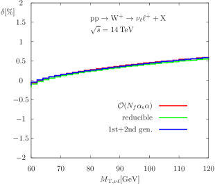
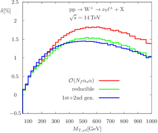
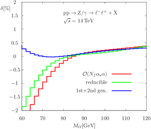
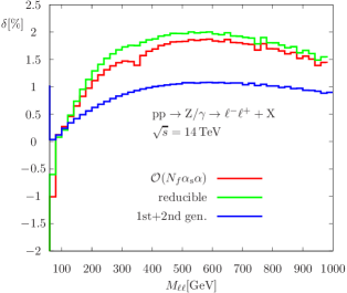
Figure 7: Relative ${\cal O}(N_{f}\alpha_{\mathrm{s}}\alpha)$ corrections to distributions in the transverse invariant mass of the W bosons (upper plots) and in the invariant mass of the Z boson (lower plots), where the complete ${\cal O}(N_{f}\alpha_{\mathrm{s}}\alpha)$ corrections are compared to the contribution originating from reducible graphs and to the contribution delivered by the first two fermion generations.

In the calculation of $\delta$ the ${\cal O}(N_{f}\alpha_{\mathrm{s}}\alpha)$ contribution ${\mathrm{d}}\sigma_{(N_{f}\alpha_{\mathrm{s}}\alpha)}$ to the differential cross section is normalized to the LO cross section ${\mathrm{d}}\sigma_{\mathrm{LO}}$ bin by bin in the histograms, where both contributions are evaluated with the same PDF set, so that $\delta$ is practically independent of the factorization scale $\mu_{\mathrm{F}}$. The correction $\delta$ mildly depends on the renormalization scale $\mu_{\mathrm{R}}$ via its proportionality to $\alpha_{\mathrm{s}}(\mu_{\mathrm{R}})$. Apart from the full ${\cal O}(N_{f}\alpha_{\mathrm{s}}\alpha)$ contribution (red curves) we show the part of the correction that is furnished by reducible diagrams only (green curves) and the contribution delivered by the first two fermion generations (blue curves). In Fig. 7 we depict the regions of low and high $M_{\ell\ell}$ and $M_{{\mathrm{T}},\nu\ell}$ separately, where the resonant contributions of the intermediate W/Z bosons is contained in the low-mass plots on the l.h.s.. More precisely, the whole region with $M_{{\mathrm{T}},\nu\ell}\mathrel{\raisebox{-3.00003pt}{$\stackrel{{\scriptstyle\displaystyle<}}{{\sim}}$}}M_{\mathrm{W}}$ is dominated by resonant W bosons, while the Z-boson resonance shows up only for $M_{\ell\ell}\sim M_{\mathrm{Z}}$. We only show the relative corrections $\delta$ to illustrate their impact; results on the absolute predictions for the shown spectra and their distinctive shapes are discussed in numerous papers (see, e.g., Refs. [18, 19]). As already expected from the size of the renormalization constants given in Tab. 1, from the results on ${\cal O}(\alpha_{\mathrm{s}}\alpha)$ corrections for stable W/Z bosons, and from the results in pole approximation [44], the impact of ${\cal O}(N_{f}\alpha_{\mathrm{s}}\alpha)$ corrections is at the level of permille, and thus phenomenologically unimportant, in all regions where resonant W/Z bosons dominate the cross section. Away from the resonance regions, the corrections grow to 1.5–2%, which is the typical size of the corrections for $M_{\ell\ell}$ and $M_{{\mathrm{T}},\nu\ell}$ values of $300{-}1000\,\mathrm{GeV}$. Corrections of this size are in fact phenomenologically relevant in those off-shell tails, in particular in the search for traces of new physics, as potentially induced by ${\mathrm{Z}}^{\prime}$ or ${\mathrm{W}}^{\prime}$ bosons.

It is interesting to note that the contribution of reducible corrections dominates over the impact of irreducible diagrams whenever the ${\cal O}(N_{f}\alpha_{\mathrm{s}}\alpha)$ correction is sizeable. Furthermore, we notice that the contributions of the individual fermion generations are generically of similar size, i.e. there is no suppression of the third generation (with massive quarks) w.r.t. to the other generations. In fact for Z production the impact of the third generation is even larger than the sum of the first two. We note in passing that the ${\mathrm{t}}\bar{\mathrm{t}}$ threshold is observable in the $M_{\ell\ell}$ spectrum at $M_{\ell\ell}\sim 2m_{\mathrm{t}}\approx 346\,\mathrm{GeV}$ (lower right plot in Fig. 7) in the full ${\cal O}(N_{f}\alpha_{\mathrm{s}}\alpha)$ correction (red) and its reducible part (green), but of course not in the contribution of the first two fermion generations (blue). From the comparison of the three different curves we conclude that neither a neglect of the third quark generation nor the approximation by setting $m_{\mathrm{t}}$ and $m_{\mathrm{b}}$ to zero provides a viable approximation for the corrections. Such approximations are often useful for QCD corrections at low or high energies; for EW corrections such approximations in general fail, since the EW gauge-boson masses $M_{\mathrm{W}}\sim M_{\mathrm{Z}}$ enter the renormalization conditions and provide an additional scale.

Figure 8 shows the relative ${\cal O}(N_{f}\alpha_{\mathrm{s}}\alpha)$ correction $\delta$ to the leptonic transverse-momentum distributions in the low- and high-energy regions.

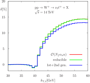
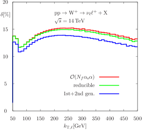
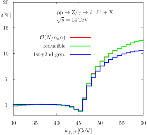
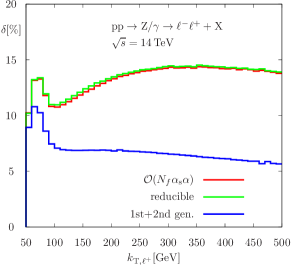
Figure 8: Relative ${\cal O}(N_{f}\alpha_{\mathrm{s}}\alpha)$ corrections to transverse-momentum distributions for W-boson (upper plots) and Z-boson production (lower plots), again with a comparison of full ${\cal O}(N_{f}\alpha_{\mathrm{s}}\alpha)$ corrections to its reducible parts and to the contribution of the first two fermion generations.

At LO, the regions in which resonant W/Z bosons dominate the spectra are characterized by $k_{{\mathrm{T}},\ell}\mathrel{\raisebox{-3.00003pt}{$\stackrel{{\scriptstyle\displaystyle<}}{{\sim}}$}}M_{V}/2$ $(V={\mathrm{W}},{\mathrm{Z}})$, i.e. at the left side of the Jacobian peaks at $k_{{\mathrm{T}},\ell}=M_{V}/2$. Note, however, that jet emission from the initial-state partons transfers some transverse momentum to the W/Z bosons, so that in the presence of QCD corrections (and to a lesser extent also in the presence of photonic corrections which are not discussed here) the $k_{{\mathrm{T}},\ell}$ regions above the Jacobian peaks receive contributions that are enhanced by a W/Z resonance. This well-known effect leads to extremely large QCD corrections for $k_{{\mathrm{T}},\ell}>M_{V}/2$ which grow to some 100%. This does not mean that perturbation theory does not work in this region, but only that the LO prediction is not a good approximation for the differential cross section there. This enhancement mechanism of NLO QCD over LO contribution also leads to an enhancement of the ${\cal O}(\alpha_{\mathrm{s}}\alpha)$ correction, since it involves jet emission as well. In Fig. 8 the suppression of the LO cross section for $k_{{\mathrm{T}},\ell}>M_{V}/2$ results in large values of $\delta$ that grow even to about $15\%$ for $k_{{\mathrm{T}},\ell}\mathrel{\raisebox{-3.00003pt}{$\stackrel{{\scriptstyle\displaystyle>}}{{\sim}}$}}250\,\mathrm{GeV}$. If we used the QCD-corrected cross section in the normalization of $\delta$, we would get relative corrections in the few-% range, which is of the expected size of the ${\cal O}(\alpha_{\mathrm{s}}\alpha)$ corrections as observed in the invariant-mass spectra above. The dominance of the real QCD corrections via the described recoil mechanism is also the reason for the extreme dominance of the reducible contributions in the ${\cal O}(N_{f}\alpha_{\mathrm{s}}\alpha)$ corrections, because the irreducible corrections do not involve real-emission effects. As already noticed in the discussion of the invariant-mass spectra above, the contribution of the third generation relative to each of the first two is higher for Z production than for W production; this feature is even more pronounced in the transverse-momentum spectra.

Finally, we mention that we observe only permille corrections of ${\cal O}(N_{f}\alpha_{\mathrm{s}}\alpha)$ to the integrated cross section and to differential distributions that are entirely dominated by resonant W or Z bosons, such as distributions in the lepton rapidities.

4 Summary

Next-to-next-to-leading-order corrections of mixed QCD$\times$EW type seem to be the largest component of the yet unknown radiative corrections to Drell–Yan-like W/Z production at fixed perturbative order, at least for off-shell W/Z bosons. In the vicinity of the W/Z resonances, the corrections are known in the form of a pole approximation up to the corrections that solely concern the initial state, which are supposed to be small. Recent evaluations of those initial-state corrections for on-shell Z bosons have confirmed this expectation. For off-shell W/Z production, several ingredients have been presented in recent years, including results for rather complex two-loop integrals, but no cross-section predictions have been presented yet. This paper takes a first step towards the numerical evaluation of the ${\cal O}(\alpha_{\mathrm{s}}\alpha)$ corrections by presenting results on the corrections of ${\cal O}(N_{f}\alpha_{\mathrm{s}}\alpha)$, which are nominally enhanced by the number $N_{f}$ of fermion generations. These corrections comprise all diagrams with closed fermion loops and form a gauge-invariant part of the full ${\cal O}(\alpha_{\mathrm{s}}\alpha)$ corrections.

The genuine two-loop part of the calculation involves only self-energy complexity and was feasible by a straightforward application of current two-loop techniques. The two-loop integrals were reduced to master integrals with the help of Laporta’s algorithm as implemented in the program KIRA, and the master integrals were evaluated via differential equations. We have successfully compared our results on the EW gauge-boson self-energies to existing results in the literature and give explicit analytical results to allow for cross-checks with upcoming similar calculations. Generally, the description of resonance processes including higher-order corrections is delicate, in particular because of issues with gauge invariance. In order to guarantee a gauge-invariant description that is uniformly valid on resonance and in off-shell regions, we have generalized the complex-mass scheme, which is a standard procedure for treating resonances at NLO. It is interesting to note that the consideration of all ${\cal O}(N_{f}\alpha_{\mathrm{s}}\alpha)$ corrections is already sufficient for the generalization of the complex-mass scheme for the full ${\cal O}(\alpha_{\mathrm{s}}\alpha)$ corrections, since the W/Z propagators that develop the resonance are affected at ${\cal O}(\alpha_{\mathrm{s}}\alpha)$ only by diagrams involving closed quark loops.

Concerning real corrections, focusing on ${\cal O}(N_{f}\alpha_{\mathrm{s}}\alpha)$ leads to drastic simplifications in comparison to the full ${\cal O}(\alpha_{\mathrm{s}}\alpha)$ corrections as well. Since the ${\cal O}(N_{f}\alpha_{\mathrm{s}}\alpha)$ corrections do not involve photon emission, but only up to a single emission of QCD partons, one-loop subtraction techniques are sufficient to treat infrared singularities. Specifically, we have applied dipole and alternatively antenna subtraction.

Our discussion on numerical results shows that ${\cal O}(N_{f}\alpha_{\mathrm{s}}\alpha)$ corrections to observables that are dominated by resonant W/Z bosons, such as integrated cross sections or rapidity distributions, are at the permille level and thus phenomenologically negligible. This could be already concluded from the existing results on on-shell W/Z production or from results in pole approximation. Off-shell regions in differential distributions, however, receive sizeable corrections. For instance, the invariant-mass distribution for lepton pairs in Z production and the respective transverse-invariant-mass distribution in W production receive corrections at the level of 1.5–2% for (transverse) invariant masses of $\sim 300{-}1000\,\mathrm{GeV}$. Nominally, transverse-momentum distributions of leptons even receive corrections of the order of 10% or more above the Jacobian peak at transverse momenta $\sim M_{V}/2$ $(V={\mathrm{W}}/{\mathrm{Z}})$ if corrections are normalized to leading-order predictions. However, those corrections reduce to the few-% level after normalizing them to full predictions, since leading-order predictions systematically underestimate the distribution above the Jacobian peaks, which is a well-known phenomenon.

Considering the remaining theoretical uncertainty induced by missing higher-order corrections to W/Z production at hadron colliders, we have to keep in mind that the still unknown ${\cal O}(\alpha_{\mathrm{s}}\alpha)$ corrections without nominal $N_{f}$ enhancement are expected to be not smaller than the corrections of ${\cal O}(N_{f}\alpha_{\mathrm{s}}\alpha)$. This is due to the enhancement of EW corrections at high energies originating from double (Sudakov) and single logarithms at NLO EW, which are known to factorize from QCD corrections in higher orders. With both NLO QCD and NLO EW corrections at the (known) level of some 10% in the TeV range of invariant masses, additional ${\cal O}(\alpha_{\mathrm{s}}\alpha)$ contributions at the few-% level can be expected. The presented results on ${\cal O}(N_{f}\alpha_{\mathrm{s}}\alpha)$, thus, do not directly reduce the current theoretical uncertainty, but represent a relevant contribution to the full ${\cal O}(\alpha_{\mathrm{s}}\alpha)$ corrections and can serve as an estimate for the order of magnitude of missing corrections at this order.

A Calculation of the master integrals via differential equations

In this appendix we briefly describe the calculation of the two-loop master integrals via differential equations, which is based on transformations of the set of master integrals into Henn’s canonical form [64, 65] and subsequent integration of the new basis integrals in terms of a Laurent expansion in $\epsilon$ including terms up to order $\epsilon^{1}$, which involve Goncharov polylogarithms (GPLs) up to weight three. We start by describing the procedure for the general case of different non-vanishing masses and present some special cases with much simpler results afterwards. The most simple case, in which all masses are zero, has also been checked by direct integration with Feynman parameters.

Apart from the results outlined in the following, we have worked out an alternative solution for the master integrals, which is based on a more involved transformation to the canonical form, but leading to somewhat simpler expressions for the integrals. Numerically the two sets of obtained master integrals are in mutual agreement.

A.1 General case of different non-vanishing masses

We first change the basis of master integrals $S_{abcde}$ used to express the 1PI parts of the EW gauge-boson self-energies to the following set of basis functions,

$$\vec{F}(s,m_{1}^{2},m_{2}^{2})={} \left(F_{1},\dots,F_{9}\right)^{\mathrm{T}},$$

$$F_{1}={} sS_{10220},$$

$$F_{2}={} \sqrt{\lambda}(S_{10220}+S_{20120}+S_{20210}),$$

$$F_{3}={} s_{+-}S_{20120}-s_{-+}S_{20210}+(m_{1}^{2}-m_{2}^{2})S_{10220},$$

$$F_{4}={} S_{00220},$$

$$F_{5}={} S_{02020},$$

$$F_{6}={} \frac{1}{2\sqrt{\lambda}}\left[(\sqrt{\lambda}-s_{-+})S_{00220}-(\sqrt{\lambda}+s_{+-})S_{02020}+2(1-2\epsilon)sS_{01120}\right],$$

$$F_{7}={} \frac{1}{2\sqrt{\lambda}}\left[(\sqrt{\lambda}-s_{-+})S_{00202}-(\sqrt{\lambda}+s_{+-})S_{00220}+2(1-2\epsilon)sS_{01102}\right],$$

$$F_{8}={} \frac{s}{\lambda}\Bigl{\{}m_{2}^{2}S_{00202}+s_{--}S_{00220}+m_{1}^{2}S_{02020}$$

$$\qquad{}-(1-2\epsilon)\Big{[}s_{-+}S_{01102}-(1-2\epsilon)sS_{01111}+s_{+-}S_{01120}\Big{]}\Bigr{\}},$$

$$F_{9}={} S_{00202},$$ (A.1)

where we have used the shorthands

$$\lambda={} s^{2}+m_{1}^{4}+m_{2}^{4}-2sm_{1}^{2}-2sm_{2}^{2}-2m_{1}^{2}m_{2}^{2},$$

$$s_{\pm\pm}={} s\pm m_{1}^{2}\pm m_{2}^{2},\qquad s_{\pm\mp}=s\pm m_{1}^{2}\mp m_{2}^{2}.$$ (A.2)

Here and in the following, squared masses are always assumed to possess an infinitesimally small negative imaginary part, i.e. $m^{2}\equiv m^{2}-{\mathrm{i}}0$. Moreover, we replace the kinematical variable $s$ in favour of the dimensionless variable $x$, which rationalizes $\sqrt{\lambda}$,

$$s=\frac{x[m_{1}^{2}(1-x)-m_{2}^{2}]}{1-x},\qquad\sqrt{\lambda}=\frac{m_{2}^{2}-m_{1}^{2}(1-x)^{2}}{1-x}.$$ (A.3)

In terms of the kinematical input, the variable $x$ is calculated according to

$$x=\left\{\begin{array}[]{lcl}(s_{+-}+\sqrt{\lambda})/(2m_{1}^{2})&\mbox{ for }&\lambda>0,\;s_{+-}\geq 0,\\ 2s/(s_{+-}-\sqrt{\lambda})&\mbox{ for }&\lambda>0,\;s_{+-}<0,\\ (s_{+-}+{\mathrm{i}}\sqrt{-\lambda})/(2m_{1}^{2})&\mbox{ for }&\lambda\leq 0,\end{array}\right.$$ (A.7)

where the two versions for $\lambda>0$ are just distinguished to improve numerical stability. In order to ensure that $s=0$, which will be our initial condition for solving the differential equation, corresponds to $x=0$, we assume $m_{2}>m_{1}$ in the following. The case $m_{2}<m_{1}$ can be handled upon interchanging the mass values before the calculation of master integrals and appropriately interchanging the obtained master integrals using the symmetry relations (2.7).

The transformation to the set of functions $\vec{F}$, which is inspired by a corresponding but simpler transformation for the one-loop bubble integral, brings the differential equation of the master integrals for the evolution in the variable $s$ (keeping the masses $m_{1},m_{2}$ constant) into the canonical form

$$\frac{\partial\vec{f}}{\partial x}=\epsilon A\vec{f},$$ (A.8)

where $\vec{f}$ results from $\vec{F}$ by some rescaling,

$$\vec{F}(s,m_{1}^{2},m_{2}^{2})=\Gamma(1+\epsilon)^{2}\left(\frac{4\pi\mu^{2}}{m_{1}^{2}}\right)^{\epsilon}\left(\frac{4\pi\mu^{2}}{m_{2}^{2}}\right)^{\epsilon}\vec{f}(x,r),\qquad r=\frac{m_{2}}{m_{1}}.$$ (A.9)

Schematically, the matrix $A$ is given by

$$A=\left(\begin{array}[]{c|c|c}\lx@intercol\hfil A_{4}\hfil\lx@intercol\vrule\lx@intercol&0_{3{\times}5}\\ \cline{2-3}\cr&&\\ \cline{1-2}\cr 0_{5{\times}3}&\lx@intercol\hfil A_{6}\hfil\lx@intercol\end{array}\right),$$ (A.13)

where $A_{4}$ and $A_{6}$ are the $4\times 4$ and $6\times 6$ matrices which have the element $A_{44}=A_{4,44}=A_{6,11}=0$ in common and $0_{m\times n}$ is the zero matrix of the indicated geometry. The explicit entries of $A_{4}$ and $A_{6}$ are given by

$$A_{4}={} \begin{pmatrix}\frac{2}{x}-q(x)&\frac{1}{1-x}&0&0\\ \frac{6}{x-1}&-\frac{2}{x}-6p(x)+4q(x)&\frac{2}{1-x}+2q(x)&\frac{2}{1-x}\\ 0&\frac{1}{x-1}-q(x)&-\frac{2}{x}+q(x)&0\\ 0&0&0&0\end{pmatrix},$$

$$A_{6}={} \begin{pmatrix}0&0&0&0&0&0\\ 0&0&0&0&0&0\\ \frac{1}{1-x}+p(x)&-p(x)&q(x)-2p(x)&0&0&0\\ -p(x)&0&0&q(x)-2p(x)&0&\frac{1}{1-x}+p(x)\\ \frac{1}{1-x}+2p(x)&-p(x)&-q(x)&q(x)+\frac{2}{1-x}&2q(x)-4p(x)&\frac{1}{x-1}-p(x)\\ 0&0&0&0&0&0\end{pmatrix},$$ (A.14)

with the auxiliary functions

$$p(x)={} \frac{1}{x-1-r}+\frac{1}{x-1+r}-\frac{1}{x-1+r^{2}},$$

$$q(x)={} \frac{1}{x-1}+\frac{1}{x}-\frac{1}{x-1+r^{2}}.$$ (A.15)

Owing to the block structure (A.13) of the matrix $A$, the first four components of $\vec{f}$ and the last six components of $\vec{f}$ each define an independent system of linear differential equations, which can be solved independently; the fact that $f_{4}$ is part of either system does not disturb this feature.

As initial condition for the evolution of $\vec{f}(x,r)$ in $x$, we take the values $\vec{f}(0,r)$ corresponding to $s=0$, where the functions $S_{abcde}$ reduce to vacuum integrals of the type defined in (2.25). For the functions in $\vec{F}$ this leads to the initial values

$$F_{k}(0,m_{1}^{2},m_{2}^{2})={} 0,\quad k=1,6,7,8,$$

$$F_{2}(0,m_{1}^{2},m_{2}^{2})={} -F_{3}(0,m_{1}^{2},m_{2}^{2})=\frac{1-\epsilon}{\epsilon}\,(m_{1}^{2}-m_{2}^{2})\,T_{122}(m_{1}^{2},m_{2}^{2}),$$

$$F_{4}(0,m_{1}^{2},m_{2}^{2})={} T_{022}(m_{1}^{2},m_{2}^{2}),$$

$$F_{5}(0,m_{1}^{2},m_{2}^{2})={} T_{022}(m_{1}^{2},m_{1}^{2}),$$

$$F_{9}(0,m_{1}^{2},m_{2}^{2})={} T_{022}(m_{2}^{2},m_{2}^{2}).$$ (A.16)

The integrals $T_{022}$ are just products of simple one-loop vacuum integrals, which are easy to calculate. The integral $T_{122}$ was first expressed in terms of $T_{111}$ with the help of KIRA, and $T_{111}$ was calculated by solving the corresponding Feynman parameter integral. The result for $T_{111}$ was also checked against the one published in Ref. [95]. For the rescaled functions $\vec{f}$, the initial values explicitly read

$$f_{k}(0,r)={} 0,\quad k=1,6,7,8,$$

$$f_{2}(0,r)={} -f_{3}(0,r)$$

$$={} \frac{1}{\epsilon}\ln r^{2}-2\mathop{\mathrm{Li}}\nolimits_{2}(1-r^{-2})-\frac{1}{2}\ln^{2}r^{2}+\epsilon\left[2\mathop{\mathrm{Li}}\nolimits_{3}(1-r^{-2})-2\mathop{\mathrm{Li}}\nolimits_{3}\left(\frac{1}{1-r^{2}}\right)\right.$$

$$\left.{}+\frac{1}{3}\ln^{3}(r^{2}-1)+\frac{\pi^{2}}{3}\ln(r^{2}-1)-\frac{1}{6}\ln^{3}r^{2}\right]+{\cal O}(\epsilon^{2}),$$

$$f_{4}(0,r)={} \frac{1}{\epsilon^{2}},\qquad f_{5}(0,r)=\frac{r^{2\epsilon}}{\epsilon^{2}},\qquad f_{9}(0,r)=\frac{r^{-2\epsilon}}{\epsilon^{2}}.$$ (A.17)

With these initial values, the integration of the system (A.8) in terms of GPLs is straightforward. Since the functions $f_{k}(x,r)$ with $k=4,5,9$ are constant in $x$, their solutions are trivially given by

$$f_{k}(x,r)\equiv f_{k}(0,r),\qquad k=4,5,9.$$ (A.18)

For the remaining functions $f_{k}(x,r)$, we give the results in terms of coefficients $f^{(j)}(x,r)$ of the Laurent series

$$\vec{f}(x,r)=\sum_{j=-2}^{\infty}\epsilon^{j}\,\vec{f}^{(j)}(x,r)$$ (A.19)

up to the relevant order in $\epsilon$. Up to order $\epsilon^{0}$, those functions read

$$f_{k}^{(-2)}(x,r)={} 0,\qquad k=1,2,3,6,7,8,$$

$$f_{1}^{(-1)}(x,r)={} f_{8}^{(-1)}(x,r)=0,$$

$$f_{2}^{(-1)}(x,r)={} f_{2}^{(-1)}(0,r)-2G(1;x),$$

$$f_{3}^{(-1)}(x,r)={} f_{3}^{(-1)}(0,r),$$

$$f_{6}^{(-1)}(x,r)={} f_{7}^{(-1)}(x,r)=-G(1;x),$$

$$f_{1}^{(0)}(x,r)={} 2G(1,1;x)-G(1;x)\ln(r^{2}),$$

$$f_{2}^{(0)}(x,r)={} f_{2}^{(0)}(0,r)-4G(0,1;x)-8G(1,1;x)+12G(1-r,1;x)$$

$${}+12G(1+r,1;x)-4G(1-r^{2},1;x)$$

$${}+\big{[}4G(1;x)-6G(1-r;x)-6G(1+r;x)+4G(1-r^{2};x)\big{]}\ln(r^{2}),$$

$$f_{3}^{(0)}(x,r)={} f_{3}^{(0)}(0,r)+2G(0,1;x)-2G(1-r^{2},1;x)-\big{[}G(1;x)-2G(1-r^{2};x)\big{]}\ln(r^{2}),$$

$$f_{6}^{(0)}(x,r)={} -G(0,1;x)-G(1,1;x)+2G(1-r,1;x)+2G(1+r,1;x)-G(1-r^{2},1;x)$$

$${}-\big{[}G(1-r;x)+G(1+r;x)-G(1-r^{2};x)\big{]}\ln(r^{2}),$$

$$f_{7}^{(0)}(x,r)={} -G(0,1;x)-G(1,1;x)+2G(1-r,1;x)+2G(1+r,1;x)-G(1-r^{2},1;x)$$

$${}+\big{[}G(1;x)-G(1-r;x)-G(1+r;x)+G(1-r^{2};x)\big{]}\ln(r^{2}),$$

$$f_{8}^{(0)}(x,r)={} 2G(1,1;x)-G(1;x)\ln(r^{2}).$$ (A.20)

For the evaluation of the self-energies given in Section 2.2, the functions $f_{k}^{(1)}(x,r)$, the results of which are getting more lengthy and untransparent, are needed as well; we provide those functions in an ancillary file supplementing the online version of this article.

To finally reconstruct the relevant master integrals $S_{abcde}$ in terms of a Laurent series in powers of $\epsilon$, we first have to convert the coefficients $f_{k}^{(j)}(x,r)$ to the corresponding coefficients $F_{k}^{(j)}(s,m_{1}^{2},m_{2}^{2})$ of the components of $\vec{F}$ as defined in (A.9). By convention, we do not expand the global factor $\Gamma(1+\epsilon)^{2}\,(4\pi)^{2\epsilon}$ contained in $\vec{F}$ and define

$$F_{k}(s,m_{1}^{2},m_{2}^{2})={} \sum_{j=-2}^{\infty}\Gamma(1+\epsilon)^{2}\,(4\pi)^{2\epsilon}\,\epsilon^{j}\,F_{k}^{(j)}(s,m_{1}^{2},m_{2}^{2}),$$ (A.21)

so that

$$F_{k}^{(-2)}(s,m_{1}^{2},m_{2}^{2})={} f_{k}^{(-2)}(x,r),$$

$$F_{k}^{(-1)}(s,m_{1}^{2},m_{2}^{2})={} f_{k}^{(-1)}(x,r)+f_{k}^{(-2)}(x,r)L,$$

$$F_{k}^{(0)}(s,m_{1}^{2},m_{2}^{2})={} f_{k}^{(0)}(x,r)+L\,f_{k}^{(-1)}(x,r)+\textstyle\frac{1}{2}L^{2}\,f_{k}^{(-2)}(x,r),$$

$$F_{k}^{(1)}(s,m_{1}^{2},m_{2}^{2})={} f_{k}^{(1)}(x,r)+L\,f_{k}^{(0)}(x,r)+\textstyle\frac{1}{2}L^{2}\,f_{k}^{(-1)}(x,r)+\textstyle\frac{1}{6}L^{3}\,f_{k}^{(-2)}(x,r),$$ (A.22)

with the constant

$$L=\ln\left(\frac{\mu^{2}}{m_{1}^{2}}\right)+\ln\left(\frac{\mu^{2}}{m_{2}^{2}}\right)$$ (A.23)

containing the dependence on the reference scale $\mu$. The set of master integrals $S_{abcde}$ contained in (A.1) can be derived from the results for $F_{k}(s,m_{1}^{2},m_{2}^{2})$ by simply inverting the set of linear equations (A.1). The corresponding results for the Laurent coefficients defined by

$$S_{abcde}(s,m_{1}^{2},m_{2}^{2})={} \sum_{j=-2}^{\infty}\Gamma(1+\epsilon)^{2}\,(4\pi)^{2\epsilon}\,\epsilon^{j}\,S_{abcde}^{(j)}(s,m_{1}^{2},m_{2}^{2}),$$ (A.24)

in terms of the $F_{k}^{(j)}$, however, get somewhat lengthy because of the explicit appearance of $\epsilon$ in the defining equations. Moreover, the basis set of master integrals used in the self-energies in Section 2.2 is not identical with the one used in (A.1), i.e. a further change of basis has to be performed. Instead of reproducing unnecessarily lengthy formulas here, we provide the coefficients $S_{abcde}^{(j)}$ needed for the self-energies in terms of the coefficients $F_{k}^{(j)}$ given above in the mentioned ancillary file.

A.2 Two equal non-vanishing masses

In this appendix we consider the calculation of the master integrals $S_{abcde}$ for the special case $m=m_{1}=m_{2}$, in which the number of independent master integrals is reduced compared to the general case of the previous section owing to the symmetry relations (2.7). To solve the system of differential equations obeyed by those master integrals we consider the following basis of five functions,

$$\vec{F}(s,m^{2})={} \left(F_{1},\dots,F_{5}\right)^{\mathrm{T}},$$

$$F_{1}={} sS_{10220},$$

$$F_{2}={} \sqrt{\lambda}(S_{10220}+S_{20120}+S_{20210}),$$

$$F_{3}={} S_{02020},$$

$$F_{4}={} \frac{s}{\sqrt{\lambda}}\big{[}(1-2\epsilon)S_{01120}-S_{02020}\big{]},$$

$$F_{5}={} \frac{s^{2}}{\lambda}\big{[}(1-2\epsilon)^{2}S_{01111}-2(1-2\epsilon)S_{01120}+S_{02020}\big{]},$$ (A.25)

with the shorthand

$$\lambda={} s^{2}-4sm^{2}.$$ (A.26)

We replace the kinematical variable $s$ in favour of the dimensionless variable $x$, which rationalizes $\sqrt{\lambda}$,

$$s=\frac{m^{2}x^{2}}{x-1},\qquad\sqrt{\lambda}=\frac{m^{2}x(x-2)}{x-1}.$$ (A.27)

In terms of the kinematical input, the variable $x$ is calculated according to

$$x=\left\{\begin{array}[]{lll}(s+\sqrt{\lambda})/(2m^{2})&\mbox{ for }&s>4m^{2},\\ 2s/(s-\sqrt{\lambda})&\mbox{ for }&s<0,\\ (s+{\mathrm{i}}\sqrt{-\lambda})/(2m^{2})&\hbox to0.0pt{ otherwise.\hss}&\end{array}\right.$$ (A.31)

Rescaling $\vec{F}$ according to

$$\vec{F}(s,m^{2})=\Gamma(1+\epsilon)^{2}\left(\frac{4\pi\mu^{2}}{m^{2}}\right)^{2\epsilon}\vec{f}(x),$$ (A.32)

the functions $\vec{f}$ fulfill a differential equation of the form (A.8) with the matrix $A$ schematically given by

$$A=\left(\begin{array}[]{c|c|c}\lx@intercol\hfil A_{3}\hfil\lx@intercol\vrule\lx@intercol&0_{2{\times}2}\\ \cline{2-3}\cr&&\\ \cline{1-2}\cr 0_{2{\times}2}&\lx@intercol\hfil A^{\prime}_{3}\hfil\lx@intercol\end{array}\right).$$ (A.36)

The two $3\times 3$ submatrices explicitly read

$$A_{3}={} \begin{pmatrix}\frac{1}{1-x}+\frac{2}{x}&\frac{1}{1-x}&0\\ \frac{6}{x-1}&\frac{6}{2-x}+\frac{4}{x-1}-\frac{2}{x}&\frac{2}{1-x}\\ 0&0&0\end{pmatrix},$$

$$A^{\prime}_{3}={} \begin{pmatrix}0&0&0\\ \frac{1}{1-x}&\frac{2}{2-x}+\frac{1}{x-1}&0\\ 0&\frac{2}{1-x}&\frac{4}{2-x}+\frac{2}{x-1}\end{pmatrix}$$ (A.37)

and have the element $A_{33}=A_{3,33}=A^{\prime}_{3,11}=0$ in common. Each of the matrices $A_{3}$, $A^{\prime}_{3}$ defines a 3-dimensional system of linear ordinary differential equations that can be solved independently.

An appropriate initial condition is again given by $s=0$, corresponding to $x=0$, where the master integrals $S_{abcde}$ reduce to vacuum integrals. The initial values of $\vec{F}$ are given by

$$F_{3}(0,m^{2})=T_{022}(m^{2},m^{2}),\qquad F_{k}(0,m^{2})=0,\quad k=1,2,4,5,$$ (A.38)

so that

$$f_{3}(0)=\frac{1}{\epsilon^{2}},\qquad f_{k}(0)=0,\quad k=1,2,4,5.$$ (A.39)

The system of differential equations easily integrates to GPLs. Since $f_{3}(x)$ is constant in $x$, we simply have

$$f_{3}(x)\equiv f_{3}(0).$$ (A.40)

The results for the remaining $f_{k}(x)$ are given in terms of Laurent coefficients defined analogously to (A.19) up to the relevant order in $\epsilon$,

$$f_{k}^{(-2)}(x)={} 0,\qquad k=1,2,4,5,$$

$$f_{1}^{(-1)}(x)={} f_{5}^{(-1)}(x)=0,$$

$$f_{2}^{(-1)}(x)={} -2G(1;x),$$

$$f_{4}^{(-1)}(x)={} -G(1;x),$$

$$f_{1}^{(0)}(x)={} f_{5}^{(0)}(x)=2G(1,1;x),$$

$$f_{2}^{(0)}(x)={} 4G(0,1;x)-8G(1,1;x)+12G(2,1;x),$$

$$f_{4}^{(0)}(x)={} -G(1,1;x)+2G(2,1;x),$$

$$f_{1}^{(1)}(x)={} 4G(0,1,1;x)-4G(1,0,1;x)+6G(1,1,1;x)-12G(1,2,1;x),$$

$$f_{2}^{(1)}(x)={} -8G(0,0,1;x)+16G(0,1,1;x)-24G(0,2,1;x)+16G(1,0,1;x)$$

$${}-20G(1,1,1;x)+48G(1,2,1;x)-24G(2,0,1;x)+48G(2,1,1;x)$$

$${}-72G(2,2,1;x),$$

$$f_{4}^{(1)}(x)={} -G(1,1,1;x)+2G(1,2,1;x)+2G(2,1,1;x)-4G(2,2,1;x),$$

$$f_{5}^{(1)}(x)={} 6G(1,1,1;x)-4G(1,2,1;x)-8G(2,1,1;x).$$ (A.41)

Analogously to (A.21), we define the Laurent coefficients $F_{k}^{(j)}$ of $\vec{F}$, so that the coefficients $F_{k}^{(j)}$ are obtained from the coefficients $f_{k}^{(j)}$ as in (A.22) with the constant

$$L=2\ln\left(\frac{\mu^{2}}{m^{2}}\right)$$ (A.42)

containing the dependence on the reference scale $\mu$. The set of master integrals $S_{abcde}$ contained in (A.25) can be derived from the results for $F_{k}(s,m^{2})$ by simply inverting the set of linear equations (A.25) and finally converted into results for the master integrals used in the self-energies in Section 2.2. The corresponding results for the Laurent coefficients $S_{abcde}^{(j)}(s,m^{2},m^{2})$, which are defined as in (A.24), are again collected in an ancillary file.

A.3 One non-vanishing mass

Here we consider the calculation of the master integrals $S_{abcde}$ for the special case $m_{1}=0$ and $m_{2}=m$, which are somewhat simpler than in the two previous cases, because no rationalization of the kinematical variables is required and some vacuum integrals become scaleless and vanish. To solve the differential equation we consider the following 5-dimensional basis of functions,

$$\vec{F}(s,m^{2})={} \left(F_{1},\dots,F_{5}\right)^{\mathrm{T}},$$

$$F_{1}={} sS_{10220},$$

$$F_{2}={} (m^{2}-s)(S_{10220}+S_{20120}+S_{20210}),$$

$$F_{3}={} (1-2\epsilon)\frac{s}{m^{2}-s}S_{01102}+\frac{(s+m^{2})}{2(s-m^{2})}S_{00202}+\frac{1}{2}S_{00202},$$

$$F_{4}={} (1-2\epsilon)^{2}\frac{s^{2}}{(s-m^{2})^{2}}S_{01111}-(1-2\epsilon)\frac{s(s+m^{2})}{(s-m^{2})^{2}}S_{01102}+\frac{(s+m^{2})^{2}}{4(s-m^{2})^{2}}S_{00202}$$

$${}-\frac{1}{4}S_{00202},$$

$$F_{5}={} S_{00202}.$$ (A.43)

We replace the kinematical variable $s$ in favour of the dimensionless variable $x$,

$$s=\frac{m^{2}x}{x-1},\qquad x=\frac{s}{s-m^{2}}.$$ (A.44)

Rescaling $\vec{F}$ according to (A.32), the functions $\vec{f}$ fulfill a differential equation of the form (A.8) with the matrix $A$ schematically given by

$$A=\left(\begin{array}[]{c|c}A_{2}&0_{2{\times}3}\\ \hline\cr 0_{3{\times}2}&A_{3}\end{array}\right).$$ (A.47)

The $2\times 2$ and $3\times 3$ submatrices $A_{2}$ and $A_{3}$ explicitly read

$$A_{2}=\begin{pmatrix}\frac{1}{1-x}+\frac{1}{x}&\frac{1}{1-x}\\ \frac{6}{x-1}-\frac{6}{x}&\frac{4}{x-1}\end{pmatrix},\qquad A_{3}=\begin{pmatrix}\frac{1}{x-1}+\frac{1}{x}&0&\frac{1}{1-x}\\ \frac{1}{1-x}+\frac{1}{x}&\frac{2}{x-1}+\frac{2}{x}&\frac{1}{x-1}\\ 0&0&0\end{pmatrix}.$$ (A.48)

Each of the matrices $A_{2}$, $A_{3}$ define independent sets of linear ordinary differential equations.

An appropriate initial condition is again given by $s=0$, corresponding to $x=0$, where the master integrals $S_{abcde}$ reduce to vacuum integrals. The initial values of $\vec{F}$ are given by

$$F_{2}(0,m^{2})={} -\frac{1-\epsilon}{\epsilon}\,m^{2}\,T_{122}(0,m^{2}),\qquad F_{5}(0,m^{2})=T_{022}(0,m^{2}),$$

$$F_{k}(0,m^{2})={} 0,\quad k=1,3,4,$$ (A.49)

so that the initial values of $\vec{f}$, which are related to the ones of $\vec{F}$ according to (A.32), read

$$f_{2}(0)=-\frac{1}{\epsilon^{2}}-\frac{\pi^{2}}{3}+2\zeta(3)\epsilon+{\cal O}(\epsilon^{2}),\qquad f_{5}(0)=\frac{1}{\epsilon^{2}},\qquad f_{k}(0)=0,\quad k=1,3,4.$$ (A.50)

The system of differential equations again easily integrates to GPLs. Since $f_{5}(x)$ is constant in $x$, we simply have

$$f_{5}(x)\equiv f_{5}(0).$$ (A.51)

The results for the remaining $f_{k}(x)$ are given in terms of Laurent coefficients defined analogously to (A.19) up to the relevant order in $\epsilon$,

$$f_{2}^{(-2)}(x)={} -1,\qquad f_{k}^{(-2)}(x)=0,\qquad k=1,3,4,$$

$$f_{1}^{(-1)}(x)={} -f_{3}^{(-1)}(x)=f_{4}^{(-1)}(x)=G(1;x),$$

$$f_{2}^{(-1)}(x)={} -4G(1;x),$$

$$f_{1}^{(0)}(x)={} f_{4}^{(0)}(x)=G(0,1;x)+3G(1,1;x),$$

$$f_{2}^{(0)}(x)={} -\frac{\pi^{2}}{3}-6G(0,1;x)-10G(1,1;x),$$

$$f_{3}^{(0)}(x)={} -G(0,1;x)-G(1,1;x),$$

$$f_{1}^{(1)}(x)={} \frac{\pi^{2}}{3}\,G(1;x)+G(0,0,1;x)+3G(0,1,1;x)+5G(1,0,1;x)+7G(1,1,1;x),$$

$$f_{2}^{(1)}(x)={} 2\zeta(3)-\frac{4\pi^{2}}{3}G(1;x)-6G(0,0,1;x)-18G(0,1,1;x)-18G(1,0,1;x)$$

$${}-22G(1,1,1;x),$$

$$f_{3}^{(1)}(x)={} -G(0,0,1;x)-G(0,1,1;x)-G(1,0,1;x)-G(1,1,1;x),$$

$$f_{4}^{(1)}(x)={} G(0,0,1;x)+5G(0,1,1;x)+3G(1,0,1;x)+7G(1,1,1;x).$$ (A.52)

The Laurent coefficients $F_{k}^{(j)}$ of $\vec{F}$ are again defined as in (A.21) and obtained from the coefficients $f_{k}^{(j)}$ as in (A.22) with the constant $L$ as given in (A.42). The Laurent coefficients $S_{abcde}^{(j)}(s,0,m^{2})$ of the master integrals $S_{abcde}$ that are eventually required for the evaluation of self-energies in Section 2.2 are obtained by first constructing the integrals $S_{abcde}$ contained in (A.43) and subsequently switching to the desired basis of master integrals. The results that express the desired $S_{abcde}^{(j)}(s,0,m^{2})$ in terms of the coefficients $F_{k}^{(j)}$ constructed above are again provided in an ancillary file.

A.4 Massless case

The required master integrals for $m_{1}=m_{2}=0$ can be obtained upon specializing the results from the previous section or via Feynman parameter integration in a straightforward way. The independent integrals are explicitly given by

$$S_{10110}={} \Gamma(1+\epsilon)^{2}\left(\frac{4\pi\mu^{2}}{-s-{\mathrm{i}}0}\right)^{2\epsilon}s\left[-\frac{1}{4\epsilon}-\frac{13}{8}+\left(-\frac{115}{16}+\frac{\pi^{2}}{12}\right)\epsilon\right]+{\cal O}(\epsilon^{2}),$$

$$S_{11110}={} \Gamma(1+\epsilon)^{2}\left(\frac{4\pi\mu^{2}}{-s-{\mathrm{i}}0}\right)^{2\epsilon}\left[\frac{1}{2\epsilon^{2}}+\frac{5}{2\epsilon}+\frac{19}{2}-\frac{\pi^{2}}{6}+\left(\frac{65}{2}-\frac{5\pi^{2}}{6}-5\zeta(3)\right)\epsilon\right]+{\cal O}(\epsilon^{2}),$$

$$S_{01111}={} \Gamma(1+\epsilon)^{2}\left(\frac{4\pi\mu^{2}}{-s-{\mathrm{i}}0}\right)^{2\epsilon}\left[\frac{1}{\epsilon^{2}}+\frac{4}{\epsilon}+12-\frac{\pi^{2}}{3}+\left(32-\frac{4\pi^{2}}{3}-4\zeta(3)\right)\epsilon\right]+{\cal O}(\epsilon^{2}),$$

$$S_{01102}={} S_{00202}=S_{00220}=0.$$ (A.53)

The remaining ones follow from those via the symmetry relations (2.7).

References

- [1] TeV4LHC Working Group Collaboration, S. Abdullin et al., Tevatron-for-LHC Report: Preparations for Discoveries, 8, 2006. hep-ph/0608322.
- [2] TeV4LHC-Top, Electroweak Working Group Collaboration, C. Gerber et al., Tevatron-for-LHC Report: Top and Electroweak Physics, 5, 2007. arXiv:0705.3251.
- [3] M. Dittmar, F. Pauss, and D. Zurcher, Towards a precise parton luminosity determination at the CERN LHC, Phys. Rev. D 56 (1997) 7284–7290, [hep-ex/9705004].
- [4] V. A. Khoze, A. D. Martin, R. Orava, and M. Ryskin, Luminosity monitors at the LHC, Eur. Phys. J. C 19 (2001) 313–322, [hep-ph/0010163].
- [5] M. Boonekamp, F. Chevallier, C. Royon, and L. Schoeffel, Understanding the Structure of the Proton: From HERA and Tevatron to LHC, Acta Phys. Polon. B 40 (2009) 2239–2321, [arXiv:0902.1678].
- [6] ATLAS Collaboration, M. Aaboud et al., Measurement of the -boson mass in pp collisions at TeV with the ATLAS detector, Eur. Phys. J. C 78 (2018) 110, [arXiv:1701.07240]. [Erratum: Eur.Phys.J.C 78, 898 (2018)].
- [7] CMS Collaboration, A. M. Sirunyan et al., Measurement of the weak mixing angle using the forward-backward asymmetry of Drell-Yan events in pp collisions at 8 TeV, Eur. Phys. J. C 78 (2018) 701, [arXiv:1806.00863].
- [8] U. Baur, S. Keller, and W. Sakumoto, QED radiative corrections to boson production and the forward backward asymmetry at hadron colliders, Phys. Rev. D 57 (1998) 199–215, [hep-ph/9707301].
- [9] V. Zykunov, Electroweak corrections to the observables of W boson production at RHIC, Eur. Phys. J. direct 3 (2001) 9, [hep-ph/0107059].
- [10] U. Baur et al., Electroweak radiative corrections to neutral current Drell-Yan processes at hadron colliders, Phys. Rev. D 65 (2002) 033007, [hep-ph/0108274].
- [11] S. Dittmaier and M. Krämer, Electroweak radiative corrections to W boson production at hadron colliders, Phys. Rev. D 65 (2002) 073007, [hep-ph/0109062].
- [12] U. Baur and D. Wackeroth, Electroweak radiative corrections to beyond the pole approximation, Phys. Rev. D 70 (2004) 073015, [hep-ph/0405191].
- [13] A. Arbuzov et al., One-loop corrections to the Drell-Yan process in SANC. I. The Charged current case, Eur. Phys. J. C 46 (2006) 407–412, [hep-ph/0506110]. [Erratum: Eur.Phys.J.C 50, 505 (2007)].
- [14] C. Carloni Calame, G. Montagna, O. Nicrosini, and A. Vicini, Precision electroweak calculation of the charged current Drell-Yan process, JHEP 12 (2006) 016, [hep-ph/0609170].
- [15] V. Zykunov, Weak radiative corrections to Drell-Yan process for large invariant mass of di-lepton pair, Phys. Rev. D 75 (2007) 073019, [hep-ph/0509315].
- [16] C. Carloni Calame, G. Montagna, O. Nicrosini, and A. Vicini, Precision electroweak calculation of the production of a high transverse-momentum lepton pair at hadron colliders, JHEP 10 (2007) 109, [arXiv:0710.1722].
- [17] A. Arbuzov, et al., One-loop corrections to the Drell–Yan process in SANC. (II). The Neutral current case, Eur. Phys. J. C 54 (2008) 451–460, [arXiv:0711.0625].
- [18] S. Brensing, S. Dittmaier, M. Krämer, and A. Mück, Radiative corrections to boson hadroproduction: Higher-order electroweak and supersymmetric effects, Phys. Rev. D 77 (2008) 073006, [arXiv:0710.3309].
- [19] S. Dittmaier and M. Huber, Radiative corrections to the neutral-current Drell-Yan process in the Standard Model and its minimal supersymmetric extension, JHEP 01 (2010) 060, [arXiv:0911.2329].
- [20] R. Boughezal, Y. Li, and F. Petriello, Disentangling radiative corrections using the high-mass Drell-Yan process at the LHC, Phys. Rev. D 89 (2014) 034030, [arXiv:1312.3972].
- [21] W. Placzek and S. Jadach, Multiphoton radiation in leptonic W boson decays, Eur. Phys. J. C 29 (2003) 325–339, [hep-ph/0302065].
- [22] C. Carloni Calame, G. Montagna, O. Nicrosini, and M. Treccani, Higher order QED corrections to W boson mass determination at hadron colliders, Phys. Rev. D 69 (2004) 037301, [hep-ph/0303102].
- [23] R. Hamberg, W. van Neerven, and T. Matsuura, A complete calculation of the order correction to the Drell-Yan factor, Nucl. Phys. B 359 (1991) 343–405. [Erratum: Nucl.Phys.B 644, 403–404 (2002)].
- [24] R. Gavin, Y. Li, F. Petriello, and S. Quackenbush, W Physics at the LHC with FEWZ 2.1, Comput. Phys. Commun. 184 (2013) 208–214, [arXiv:1201.5896].
- [25] R. Gavin, Y. Li, F. Petriello, and S. Quackenbush, FEWZ 2.0: A code for hadronic Z production at next-to-next-to-leading order, Comput. Phys. Commun. 182 (2011) 2388–2403, [arXiv:1011.3540].
- [26] S. Catani et al., Vector boson production at hadron colliders: a fully exclusive QCD calculation at NNLO, Phys. Rev. Lett. 103 (2009) 082001, [arXiv:0903.2120].
- [27] K. Melnikov and F. Petriello, Electroweak gauge boson production at hadron colliders through , Phys. Rev. D 74 (2006) 114017, [hep-ph/0609070].
- [28] K. Melnikov and F. Petriello, The boson production cross section at the LHC through , Phys. Rev. Lett. 96 (2006) 231803, [hep-ph/0603182].
- [29] C. Anastasiou, L. J. Dixon, K. Melnikov, and F. Petriello, High precision QCD at hadron colliders: Electroweak gauge boson rapidity distributions at NNLO, Phys. Rev. D 69 (2004) 094008, [hep-ph/0312266].
- [30] R. V. Harlander and W. B. Kilgore, Next-to-next-to-leading order Higgs production at hadron colliders, Phys. Rev. Lett. 88 (2002) 201801, [hep-ph/0201206].
- [31] T. Ahmed, M. Mahakhud, N. Rana, and V. Ravindran, Drell-Yan Production at Threshold to Third Order in QCD, Phys. Rev. Lett. 113 (2014) 112002, [arXiv:1404.0366].
- [32] S. Catani et al., Threshold resummation at N3LL accuracy and soft-virtual cross sections at N3LO, Nucl. Phys. B 888 (2014) 75–91, [arXiv:1405.4827].
- [33] M. Guzzi, P. M. Nadolsky, and B. Wang, Nonperturbative contributions to a resummed leptonic angular distribution in inclusive neutral vector boson production, Phys. Rev. D 90 (2014) 014030, [arXiv:1309.1393].
- [34] A. Kulesza and W. Stirling, Soft gluon resummation in transverse momentum space for electroweak boson production at hadron colliders, Eur. Phys. J. C 20 (2001) 349–356, [hep-ph/0103089].
- [35] S. Catani, D. de Florian, G. Ferrera, and M. Grazzini, Vector boson production at hadron colliders: transverse-momentum resummation and leptonic decay, JHEP 12 (2015) 047, [arXiv:1507.06937].
- [36] C. Balazs and C. Yuan, Soft gluon effects on lepton pairs at hadron colliders, Phys. Rev. D 56 (1997) 5558–5583, [hep-ph/9704258].
- [37] F. Landry, R. Brock, P. M. Nadolsky, and C. Yuan, Tevatron Run-1 boson data and Collins-Soper-Sterman resummation formalism, Phys. Rev. D 67 (2003) 073016, [hep-ph/0212159].
- [38] G. Bozzi et al., Production of Drell-Yan lepton pairs in hadron collisions: Transverse-momentum resummation at next-to-next-to-leading logarithmic accuracy, Phys. Lett. B 696 (2011) 207–213, [arXiv:1007.2351].
- [39] S. Mantry and F. Petriello, Transverse Momentum Distributions from Effective Field Theory with Numerical Results, Phys. Rev. D 83 (2011) 053007, [arXiv:1007.3773].
- [40] T. Becher, M. Neubert, and D. Wilhelm, Electroweak Gauge-Boson Production at Small : Infrared Safety from the Collinear Anomaly, JHEP 02 (2012) 124, [arXiv:1109.6027].
- [41] C. Duhr, F. Dulat, and B. Mistlberger, Charged Current Drell-Yan Production at N3LO, arXiv:2007.13313.
- [42] S. Alioli et al., Precision studies of observables in and processes at the LHC, Eur. Phys. J. C 77 (2017) 280, [arXiv:1606.02330].
- [43] S. Dittmaier, A. Huss, and C. Schwinn, Mixed QCD-electroweak O(s) corrections to Drell-Yan processes in the resonance region: pole approximation and non-factorizable corrections, Nucl. Phys. B 885 (2014) 318–372, [arXiv:1403.3216].
- [44] S. Dittmaier, A. Huss, and C. Schwinn, Dominant mixed QCD-electroweak O(s) corrections to Drell–Yan processes in the resonance region, Nucl. Phys. B 904 (2016) 216–252, [arXiv:1511.08016].
- [45] A. Denner and S. Dittmaier, Electroweak Radiative Corrections for Collider Physics, Phys. Rept. 864 (2020) 1–163, [arXiv:1912.06823].
- [46] D. de Florian, M. Der, and I. Fabre, QCDQED NNLO corrections to Drell Yan production, Phys. Rev. D 98 (2018) 094008, [arXiv:1805.12214].
- [47] R. Bonciani et al., NNLO QCDEW corrections to Z production in the channel, Phys. Rev. D 101 (2020) 031301, [arXiv:1911.06200].
- [48] R. Bonciani, F. Buccioni, N. Rana, and A. Vicini, NNLO QCDEW corrections to on-shell production, arXiv:2007.06518.
- [49] M. Delto, M. Jaquier, K. Melnikov, and R. Röntsch, Mixed QCDQED corrections to on-shell boson production at the LHC, JHEP 01 (2020) 043, [arXiv:1909.08428].
- [50] F. Buccioni et al., Mixed QCD-electroweak corrections to on-shell Z production at the LHC, arXiv:2005.10221.
- [51] L. Cieri, D. de Florian, M. Der, and J. Mazzitelli, Mixed QCDQED corrections to exclusive Drell Yan production using the -subtraction method, arXiv:2005.01315.
- [52] A. Kotikov, J. H. Kuhn, and O. Veretin, Two-Loop Formfactors in Theories with Mass Gap and Z-Boson Production, Nucl. Phys. B 788 (2008) 47–62, [hep-ph/0703013].
- [53] R. Bonciani, S. Di Vita, P. Mastrolia, and U. Schubert, Two-Loop Master Integrals for the mixed EW-QCD virtual corrections to Drell-Yan scattering, JHEP 09 (2016) 091, [arXiv:1604.08581].
- [54] M. Heller, A. von Manteuffel, and R. M. Schabinger, Multiple polylogarithms with algebraic arguments and the two-loop EW-QCD Drell-Yan master integrals, arXiv:1907.00491.
- [55] S. M. Hasan and U. Schubert, Master Integrals for the mixed EW-QCD corrections to the Drell-Yan production of a massive lepton pair, arXiv:2004.14908.
- [56] A. Djouadi and P. Gambino, Electroweak gauge bosons selfenergies: Complete QCD corrections, Phys. Rev. D 49 (1994) 3499–3511, [hep-ph/9309298]. [Erratum: Phys.Rev.D 53, 4111 (1996)].
- [57] A. Djouadi and C. Verzegnassi, Virtual Very Heavy Top Effects in LEP / SLC Precision Measurements, Phys. Lett. B 195 (1987) 265–271.
- [58] A. Djouadi, O(alpha alpha-s) Vacuum Polarization Functions of the Standard Model Gauge Bosons, Nuovo Cim. A 100 (1988) 357.
- [59] T. Chang, K. Gaemers, and W. van Neerven, QCD Corrections to the Mass and Width of the Intermediate Vector Bosons, Nucl. Phys. B 202 (1982) 407–436.
- [60] B. A. Kniehl, J. H. Kühn, and R. Stuart, QCD corrections, virtual heavy quark effects and electroweak precision measurements, Phys. Lett. B 214 (1988) 621–629.
- [61] B. A. Kniehl, Two Loop Corrections to the Vacuum Polarizations in Perturbative QCD, Nucl. Phys. B 347 (1990) 86–104.
- [62] S. Laporta, High precision calculation of multiloop Feynman integrals by difference equations, Int. J. Mod. Phys. A 15 (2000) 5087–5159, [hep-ph/0102033].
- [63] P. Maierhöfer, J. Usovitsch, and P. Uwer, Kira—A Feynman integral reduction program, Comput. Phys. Commun. 230 (2018) 99–112, [arXiv:1705.05610].
- [64] J. M. Henn, Multiloop integrals in dimensional regularization made simple, Phys. Rev. Lett. 110 (2013) 251601, [arXiv:1304.1806].
- [65] J. M. Henn, Lectures on differential equations for Feynman integrals, J. Phys. A 48 (2015) 153001, [arXiv:1412.2296].
- [66] A. Denner, S. Dittmaier, M. Roth, and L. Wieders, Electroweak corrections to charged-current e+ e- 4 fermion processes: Technical details and further results, Nucl. Phys. B 724 (2005) 247–294, [hep-ph/0505042]. [Erratum: Nucl.Phys.B 854, 504–507 (2012)].
- [67] A. Arbuzov and R. Sadykov, Inverse bremsstrahlung contributions to Drell-Yan like processes, J. Exp. Theor. Phys. 106 (2008) 488–494, [arXiv:0707.0423].
- [68] S. Catani and M. Seymour, A General algorithm for calculating jet cross-sections in NLO QCD, Nucl. Phys. B 485 (1997) 291–419, [hep-ph/9605323]. [Erratum: Nucl.Phys.B 510, 503–504 (1998)].
- [69] J. Kublbeck, M. Bohm, and A. Denner, Feyn Arts: Computer Algebraic Generation of Feynman Graphs and Amplitudes, Comput. Phys. Commun. 60 (1990) 165–180.
- [70] T. Hahn, Generating Feynman diagrams and amplitudes with FeynArts 3, Comput. Phys. Commun. 140 (2001) 418–431, [hep-ph/0012260].
- [71] P. Maierhöfer and J. Usovitsch, Kira 1.2 Release Notes, arXiv:1812.01491.
- [72] A. B. Goncharov, Multiple polylogarithms, cyclotomy and modular complexes, Math. Res. Lett. 5 (1998) 497–516, [arXiv:1105.2076].
- [73] A. B. Goncharov, M. Spradlin, C. Vergu, and A. Volovich, Classical Polylogarithms for Amplitudes and Wilson Loops, Phys. Rev. Lett. 105 (2010) 151605, [arXiv:1006.5703].
- [74] E. Remiddi and J. Vermaseren, Harmonic polylogarithms, Int. J. Mod. Phys. A 15 (2000) 725–754, [hep-ph/9905237].
- [75] H. Frellesvig, D. Tommasini, and C. Wever, On the Reduction and Evaluation of Generalized Polylogarithms, PoS LL2016 (2016) 040, [arXiv:1609.00148].
- [76] S. Buehler and C. Duhr, CHAPLIN - Complex Harmonic Polylogarithms in Fortran, Comput. Phys. Commun. 185 (2014) 2703–2713, [arXiv:1106.5739].
- [77] A. Daleo, T. Gehrmann, and D. Maitre, Antenna subtraction with hadronic initial states, JHEP 04 (2007) 016, [hep-ph/0612257].
- [78] P. Nogueira, Automatic Feynman graph generation, J. Comput. Phys. 105 (1993) 279–289.
- [79] M. Steinhauser, MATAD: A Program package for the computation of MAssive TADpoles, Comput. Phys. Commun. 134 (2001) 335–364, [hep-ph/0009029].
- [80] R. Mertig, M. Böhm, and A. Denner, Feyn Calc: Computer algebraic calculation of Feynman amplitudes, Comput. Phys. Commun. 64 (1991) 345–359.
- [81] V. Shtabovenko, R. Mertig, and F. Orellana, New Developments in FeynCalc 9.0, Comput. Phys. Commun. 207 (2016) 432–444, [arXiv:1601.01167].
- [82] C. W. Bauer, A. Frink, and R. Kreckel, Introduction to the GiNaC framework for symbolic computation within the C++ programming language, J. Symb. Comput. 33 (2002) 1–12, [cs/0004015].
- [83] A. Denner, Techniques for calculation of electroweak radiative corrections at the one loop level and results for W physics at LEP-200, Fortsch. Phys. 41 (1993) 307–420, [arXiv:0709.1075].
- [84] B. S. DeWitt, Quantum Theory of Gravity. 2. The Manifestly Covariant Theory, Phys. Rev. 162 (1967) 1195–1239.
- [85] B. S. DeWitt, A gauge invariant effective action, in Oxford Conference on Quantum Gravity, pp. 449–487, 7, 1980.
- [86] G. ’t Hooft, The Background Field Method in Gauge Field Theories, in 12th Annual Winter School of Theoretical Physics, pp. 345–369, 1, 1975.
- [87] D. G. Boulware, Gauge Dependence of the Effective Action, Phys. Rev. D 23 (1981) 389.
- [88] L. Abbott, The Background Field Method Beyond One Loop, Nucl. Phys. B 185 (1981) 189–203.
- [89] A. Denner, G. Weiglein, and S. Dittmaier, Application of the background field method to the electroweak standard model, Nucl. Phys. B 440 (1995) 95–128, [hep-ph/9410338].
- [90] A. Sirlin, Radiative Corrections in the Theory: A Simple Renormalization Framework, Phys. Rev. D 22 (1980) 971–981.
- [91] W. Marciano and A. Sirlin, Radiative Corrections to Neutrino Induced Neutral Current Phenomena in the Theory, Phys. Rev. D 22 (1980) 2695. [Erratum: Phys.Rev.D 31, 213 (1985)].
- [92] Particle Data Group Collaboration, J. Beringer et al., Review of Particle Physics (RPP), Phys. Rev. D 86 (2012) 010001.
- [93] R. D. Ball et al., Parton distributions with LHC data, Nucl. Phys. B 867 (2013) 244–289, [arXiv:1207.1303].
- [94] NNPDF Collaboration, R. D. Ball et al., Parton distributions with QED corrections, Nucl. Phys. B 877 (2013) 290–320, [arXiv:1308.0598].
- [95] A. I. Davydychev and J. Tausk, Two loop selfenergy diagrams with different masses and the momentum expansion, Nucl. Phys. B 397 (1993) 123–142.