Network Thermodynamical Modelling of
Bioelectrical Systems: A Bond Graph Approach

Abstract

Interactions between biomolecules, electrons and protons are essential to many fundamental processes sustaining life. It is therefore of interest to build mathematical models of these bioelectrical processes not only to enhance understanding but also to enable computer models to complement in vitro and in vivo experiments. Such models can never be entirely accurate; it is nevertheless important that the models are compatible with physical principles. Network Thermodynamics, as implemented with bond graphs, provide one approach to creating physically compatible mathematical models of bioelectrical systems. This is illustrated using simple models of ion channels, redox reactions, proton pumps and electrogenic membrane transporters thus demonstrating that the approach can be used to build mathematical and computer models of a wide range of bioelectrical systems.

Keywords

Biological system modelling; bioelectricity; redox reactions; network thermodynamics; computational systems biology.

Introduction

In recent years, it is becoming increasingly clear that bioelectricity is involved in several key processes in cell biology, from development to signalling to proliferation ^{1, 2}. As such, it plays an important role in many diseases and also forms the underlying basis of several promising treatments ^{3, 4, 5}. Moreover, there is a strong current interest in using, or modifying, microbes for generating energy in the form of electricity, hydrogen and biofuels ^{6, 7, 8}. Mathematical models can help to provide a mechanistic understanding of bioelectrical systems and also to test synthetic biology constructs in silico⁹. To avoid false conclusions, it is vital that such models are constrained by physical laws such as energy conservation. To allow the construction of large models, a modular approach based on interconnection of reusable components is essential. To aid both understanding and computer modelling, a graphical representation is helpful. The bond graph implementation of Network Thermodynamics outlined in this paper provides a systematic way of constructing mathematical models of living systems which are both modular and physically constrained and have an underlying graphical representation.

Bioelectrical systems involve two physical domains: chemistry and electricity. However, as physical domains, they are linked by the laws of physics, and in particular by the common currency of energy. This energy-based approach provides a unifying framework to model bioelectrical systems. Engineering has several ways of modelling multi-physics energetic systems; one such method is the bond graph methodology ^{10, 11, 12, 13}. This approach was extended some 50 years ago as an energy-based approach to modelling biomolecular systems ^{14, 15, 16}. As noted by Perelson ¹⁶, the bond graph approach combines multi-physics modelling with graphical approaches from electrical circuit theory: “Graphical representations similar to engineering circuit diagrams can be constructed for thermodynamic systems. Although the proverb that a picture is worth a thousand words may not be completely applicable, such diagrams do increase one’s intuition about system behaviour. Moreover, as in circuit theory, one can algorithmically read the algebraic and differential equations that describe the system directly from the diagram much more easily than they can be constructed directly.”.

	Electrical	Chemical
Potential	Voltage	Gibbs energy
	$V~{}$\mathrm{J}\text{\,}{\mathrm{C}}^{-1}$$ or $\mathrm{V}$	$\mu~{}$\mathrm{J}\text{\,}{\mathrm{mol}}^{-1}$$
Flow	Current	Molar flow
	$i~{}$\mathrm{C}\text{\,}{\mathrm{s}}^{-1}$$ or $\mathrm{A}$	$v~{}$\mathrm{mol}\text{\,}{\mathrm{s}}^{-1}$$
Quantity	Charge	Moles
	$Q~{}$\mathrm{C}$$ where $i=\dot{Q}$	$q~{}$\mathrm{mol}$$ where $v=\dot{q}$
Capacitance C	$V=\dfrac{Q}{C}$	$\mu=\mu^{\ominus}+RT\ln\frac{q}{q^{\ominus}}$
Resistance Re	$i=\dfrac{V_{f}-V_{r}}{\rho}$	$v=\kappa\left(e^{\frac{\mu_{f}}{RT}}-e^{\frac{\mu_{r}}{RT}}\right)$

Table 1: Analogies and Energy-based modelling. In both electrical and chemical domains: $potential\times flow=power~{}$\mathrm{J}\text{\,}{\mathrm{s}}^{-1}$$. $\mu^{\ominus}$ and $q^{\ominus}$ refer to standard conditions, $RT$ is the product of the gas constant and temperature and subscripts $f$ and $r$ abbreviate forward and reverse.

The Network Thermodynamic approach can be applied not only to the chemical properties but also to the electrical properties of biomolecular systems in a uniform manner. Indeed, the bond graph approach can be seen as a formal approach to the concept of physical analogies introduced by James Clerk Maxwell¹⁷ who pointed out that analogies are central to scientific thinking and allow mathematical results and intuition from one domain to be transferred to another – see Table 1. An issue that arises in multi-physics models is the different dimensions and units used in each domain. For example, mechanical systems use force ($\mathrm{N}$) and velocity ($\mathrm{m}\text{\,}{\mathrm{s}}^{-1}$), electrical systems use voltage ($\mathrm{V}$) and current ($\mathrm{A}$) and chemical systems use chemical potential ($\mu~{}$\mathrm{J}\text{\,}{\mathrm{mol}}^{-1}$$) and molar flow ($v~{}$\mathrm{mol}\text{\,}{\mathrm{s}}^{-1}$$).

Despite these differences, the product of the two physical covariables in each of these three examples is energy flow ($\mathrm{J}\text{\,}{\mathrm{s}}^{-1}$) . It is therefore clear that the common quantity among all physical domains is energy ($\mathrm{J}$). The commonality of energy over different physical domains makes the bond graph approach appropriate for modelling multi-domain systems, in particular bioelectrical systems ^{18, 19}. Noting that the conversion factor relating the electrical and chemical domains is Faraday’s constant $F\approx$96\,485\text{\,}\mathrm{C}\,\mathrm{m}\mathrm{o}\mathrm{l}^{-1}$$, the chemical covariables $\mu$ and $v$ may be scaled by $F$ to give the pair of covariables $\phi$ (Faraday-equivalent chemical potential) and $f$ (Faraday-equivalent flow) in electrical units¹⁹:

$$\phi =\frac{\mu}{F}~{}($\mathrm{V}$)$$ (1)

$$\text{and }f =Fv~{}($\mathrm{A}$)$$ (2)

This reformulation is frequently used in the bioelectrical disciplines of electrophysiology and mitochondrial energetics where it is convenient to represent quantities in terms of voltages and currents ^{20, 21, 22, 7}.

Because energy is the common quantity across physical domains, this approach allows modular construction of large multi-physical models from reusable components ^{23, 24}. Moreover, components can be replaced by simpler, but physically plausible, alternatives to aid understanding and reduce computational load ²⁵.

Equations (1)–(2) unify the description of the electrical and chemical domains of bioelectrical systems including the ion channel and redox examples treated in the sequel. These concepts are explored in the following section using electrodiffusion and ion channels as an introductory example. The potential of bond graphs in representing bioelectrical systems in a modular manner is then illustrated using a model of redox reactions and electron-driven proton pumps in the context of the mitochondrial electron transport chain. Finally, we consider the thermodynamics of electrogenic transport in a model of the sodium-glucose symporter, which is compared to experimental data.

Energy-based modelling – a brief introduction

Component	Electrical	Chemical
C	capacitor	species
Re	resistor	reaction
0	parallel connection	common potential
1	seriesl connection	common flow

Table 2: Bond graph components express the analogies of Table 1.

As noted in Table 1, both the electrical and chemical physical domains have energy (measured in Joules  ($\mathrm{J}$) ) in common. This is the fundamental idea of energy based modelling and means that both domains can be modelled within a common framework. The bond graph framework for energy-based modelling is summarised in this section and the next section takes a closer look. The four relevant bond graph components are listed in Table 2 and express the analogies of Table 1.

(a) Electrical Circuit

(b) Bond Graph

Figure 1: Analogous systems: (a) A reaction system A ¡¿ [ r1 ] B ¡¿ [ r2 ] C + D comprises two reactions r1 and r2 and four species A, D, C and D. Using the analogies of Table 1, this is analogous to the circuit diagram shown comprising two resistors $r_{1}$ and $r_{2}$ and four capacitors. (b) Using the components of Table 2, both systems have the bond graph representation shown where the two reactions or resistors are modelled by Re:$\mathbf{r1}$ and Re:$\mathbf{r2}$ and the four species or capacitors are represented by C:$\mathbf{A}$, C:$\mathbf{B}$, C:$\mathbf{C}$ and C:$\mathbf{D}$. The difference between the two domains lies in the different equations listed in Table 1. The $\rightharpoondown$ indicate energy flows of either electrical energy or chemical energy and the 0 and 1 junctions of Table 2 provide the connections.

Figure 1 shows two analogous systems, a chemical reaction system and an electrical circuit, together with the corresponding bond graph.

Bond Graph Modelling of Electrogenic Systems

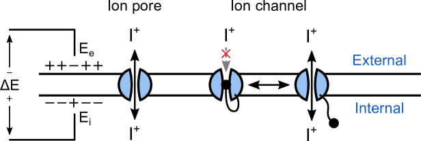
(a) Schematic

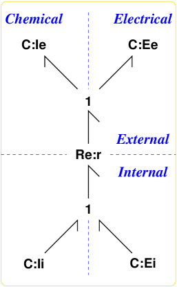
(b) Electrodiffusion

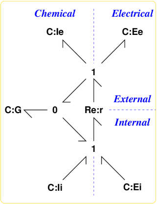
(c) Ion Channel

Figure 2: Bond Graph Modelling of Electrogenic Systems. (a) A schematic of an ion transport through a charged membrane with differential voltage $\Delta E=E_{i}-E_{e}$. A monovalent ion I+ (which could be, for example, Na+ or K+) passes though either a membrane pore (left) or an ion channel (middle and right). While the membrane pore is always open, the ion channel can switch between closed (middle) and open (right) states under the influence of a gating variable which may be either a ligand or a voltage. (b) Electrodiffusion. A monovalent ion I+ passes though a membrane pore where a flow from interior to exterior is regarded as positive. C:$\mathbf{Ii}$ represents the accumulation of the ion, and C:$\mathbf{Ei}$ represents the accumulation of charge, inside the membrane. Similarly C:$\mathbf{Ie}$ and C:$\mathbf{Ee}$ represent these quantities outside the membrane. Re:$\mathbf{r}$ represents the net effect of the pores in a given area of the membrane. The 0 and 1 components are junctions connecting two or more bonds. The 1 junction connects so that the flow is common; the 0 junction connects so that the potential is common. C components store, but do not dissipate, energy; Re components dissipate, but do not store, energy; 0 and 1 junctions transmit, but neither dissipate nor store energy. (c) Gated ion channel. The model is identical to that of (b) except the flow is gated by the potential of the gate represented by C:$\mathbf{G}$. Depending on whether the channel is ligand-gated or voltage-gated, C:$\mathbf{G}$ can represent either an accumulation of ligand or an accumulation of charge.

The bond graph representation of the network thermodynamics of chemical systems was introduced Katchalsky and coworkers ^{14, 15} and summarised by Perelson ¹⁶. In 1993, the inventor of bond graphs, Henry Paynter, said ²⁶:

Katchalsky’s breakthroughs in extending bond graphs to biochemistry are very much on my own mind. I remain convinced that BG models will play an increasingly important role in the upcoming century, applied to chemistry, electrochemistry and biochemistry, fields whose practical consequences will have a significance comparable to that of electronics in this century. This will occur both in device form, say as chemfets, biochips, etc, as well as in the basic sciences of biology, genetics, etc.

This challenge was largely ignored until recently when the bond graph approach was extended by Gawthrop and Crampin ²⁷.

The approach is introduced here in a tutorial fashion with reference to a basic bioelectrical entity: electrodiffusion though a membrane pore (Figure 2(a)). A bond graph representation appears in Figure 2(b) and explained in the following sections.

The energy bond

The $\rightharpoondown$ symbol indicates an energy bond: an energetic connection between two subsystems; the half-arrow indicates the direction corresponding to positive energy flow. In the context of this paper, the bonds carry the Faraday-equivalent covariables $\phi$ and $f$. These bonds connect four types of component: the four C components representing accumulation of chemical species (C:$\mathbf{Ie}$,C:$\mathbf{Ii}$) or electrical charge (C:$\mathbf{Ee}$,C:$\mathbf{Ei}$); an Re component representing the membrane pore; and the 1 junction connects the components via the bonds. These four components are now discussed in detail.

C component

We consider two types of C components in this paper: those corresponding to chemical species and those corresponding to electrical charge. The C components representing chemical species generate the Faraday-equivalent potential $\phi$ of Equation (1) in terms of the amount of species $x$ as¹⁹:

$$\phi =\phi^{\ominus}+\phi_{N}\ln\frac{x}{x^{\ominus}}$$ (3)

$$\text{where }\phi_{N} =\frac{RT}{F}\approx 26\ $\mathrm{m}\mathrm{V}$$$ (4)

$\phi^{\ominus}$ is the standard potential at the standard amount $x^{\ominus}$. $R=8.314\ $\mathrm{J}\text{\,}{\mathrm{K}}^{-1}\text{\,}{\mathrm{mol}}^{-1}$$ is the universal gas constant and $F$ is Faraday’s constant. The amount of species $x$ is the integral of the species Faraday-equivalent flow $f$:

$$x=\int^{t}f(\tau)d\tau$$ (5)

In some cases, it is convenient to express the potential in terms of concentration $c$ as

$$\phi =\phi^{\ominus}+\phi_{N}\ln\frac{c}{c^{\ominus}}$$ (6)

where $\phi^{\ominus}$ is the standard potential referenced to a standard concentration $c^{\ominus}$.

In contrast to the nonlinear chemical components, the C components representing electrical capacitance are linear and generate electrical potential $\phi$ (Volts) in terms of the charge $x=\int^{t}f(\tau)d\tau$ and electrical capacitance $C$ as:

$$\phi =\frac{x}{C}$$ (7)

Open systems & Chemostats

The concept of a chemostat ²⁸ provides a way of converting a closed system to an open system whilst retaining the basic closed system bond graph formulation ²³. The chemostat has a number of interpretations ²⁹:

1. one or more species is fixed to give a constant concentration; this implies that an appropriate external flow is applied to balance the internal flow of the species.

2. an ideal feedback controller is applied to species to be fixed with setpoint as the fixed concentration and control signal an external flow.

3. as a C component with a fixed state.

4. as a concentration clamp or fixed boundary condition.

The chemostatted species can be thought of as external connections turning a closed system into an open system; as such, they can be also thought of as system ports providing a point of interconnection with other systems and thus leading to a modular modelling paradigm ^{19, 23, 30}.

Re component

The R component is the bond graph abstraction of an electrical resistor. In the chemical context, a two-port R component represents a chemical reaction with chemical affinity (net chemical potential) replacing voltage and molar flow replacing current ^{14, 15}. As it is so fundamental, this two port R component is given a special symbol: Re  ²⁷.

Again, there are two versions: a non linear version corresponding to chemical systems and a linear version corresponding to electrical systems. In particular, the Re component determines a reaction flow $f$ in terms of forward and reverse reaction potentials $\Phi^{f}$ and $\Phi^{r}$ as the Marcelin – de Donder formula ³¹ rewritten in Faraday-equivalent form:

$$f =\kappa\left(\exp{\frac{{\Phi^{f}}}{\phi_{N}}}-\exp{\frac{{\Phi^{r}}}{\phi_{N}}}\right)$$ (8)

$\phi_{N}$ is given by Equation (4) and $\kappa$ is the reaction rate constant. This formulation corresponds to the mass-action formulation; other formulations are possible within this framework ^{27, 30, 25}.

The net reaction potential $\Phi$ is given in terms of the forward and reverse reaction potentials by:

$$\Phi={\Phi^{f}}-{\Phi^{r}}$$ (9)

When $\Phi=0$, the reaction is said to be at equilibrium, which also implies via Equation (8) that the flow through the reaction $f$ is zero.

0 and 1 junctions

Electrical components may be connected in parallel (where the voltage is common) and series (where the current is common). These two concepts are generalised in the bond graph notation as the 0 junction which implies that all impinging bonds have the same potential (but different flows) and the 1 junction which implies that all impinging bonds have the same flow (but different potentials). The direction of positive energy transmission is determined by the bond half arrow. As all bonds impinging on a 0 junction have the same potential, the half arrow implies the sign of the flows for each impinging bond. The reverse is true for 1 junctions, where the half arrow implies the signs of the potentials.

These components therefore describe the network topology of the system.

Electrodiffusion and the Nernst Potential

Figure 2(b) combines these bond graph components into a model of electrodiffusion: the flow of charged ions though a membrane pore. The italicised text and the dashed lines are not part of the bond graph but add the clarity of the diagram; in particular they emphasise the two divisions: internal/external and chemical/electrical.

The external compartment is modelled by two C components: C:$\mathbf{Ie}$ accumulating the external ion species as a chemical entity and C:$\mathbf{Ee}$ accumulating the external ion species as an electrical entity. The internal compartment is modelled in a similar fashion. The flow $f$ between the compartments is modelled by a single Re component; this is taken as positive if the flow is from the interior to the exterior. The upper 1 junction ensures that the flow in to both C:$\mathbf{Ie}$ and C:$\mathbf{Ee}$ is the same as that through Re:$\mathbf{r}$; the lower 1 junction ensures that the flow from both C:$\mathbf{Ie}$ and C:$\mathbf{Ee}$ is also the same as that through Re:$\mathbf{r}$.

The 0 and 1 junctions contribute to the network topology of the bond graph, which simultaneously (via 1 junctions) distributes the flow from reactions to species and potentials from species to reactions. This can be summarised in terms of the stoichiometric matrix $N$ as ²⁷:

$$\frac{d}{dt}{X} =Nf \Phi=-N^{T}\phi$$ (10)

where, in this case:

$$N =\left(\begin{matrix}1\\ -1\\ 1\\ -1\end{matrix}\right) X =\begin{pmatrix}x_{Ee}\\ x_{Ei}\\ x_{Ie}\\ x_{Ii}\\ \end{pmatrix} \phi =\begin{pmatrix}\phi_{Ee}\\ \phi_{Ei}\\ \phi_{Ie}\\ \phi_{Ii}\\ \end{pmatrix}$$ (11)

and $\Phi$ is the reaction potential (9). In this case, $\Phi$ is given by:

$$\Phi=\phi_{Ei}-\phi_{Ee}+\phi_{Ii}-\phi_{Ie}$$ (12)

Defining the membrane voltage as $\Delta E=\phi_{Ei}-\phi_{Ee}$ and using equation (6):

$$\Phi =\Delta E+\phi_{Ii}^{\ominus}+{\phi_{N}}\left(\ln\frac{c_{i}}{c_{i}^{\ominus}}\right)-\phi_{Ie}^{\ominus}-{\phi_{N}}\left(\ln\frac{c_{e}}{c_{e}^{\ominus}}\right)$$ (13)

$$=\Delta E-{\phi_{N}}\ln\frac{c_{e}}{c_{i}}$$ (14)

where we have used the equalities $\phi_{Ii}^{\ominus}=\phi_{Ie}^{\ominus}$ and $c_{i}^{\ominus}=c_{e}^{\ominus}$.

The equilibrium $\Phi=0$ occurs when the membrane potential is given by:

$$\Delta E={\phi_{N}}\ln\frac{c_{e}}{c_{i}}$$ (15)

This is the well-known formula for the Nernst potential ³².

Away from equilibrium, the flow $f$ depends on the channel characteristics and is typically modelled by the Goldman-Hodgkin-Katz equation ³² and can be implemented by suitably modifying the basic Re flow equation (8) ¹⁸.

Membrane Ion channels can be modulated (or gated) by ligands or by voltages ³³. Figure 2(c) indicates how the electrodiffusion model can be extended by adding an additional chemical C component C:$\mathbf{G}$ acting as a gate; this is directly analogous to modulating a chemical reaction with an enzyme ²⁷. The dynamics of such gates may also be modelled using the bond graph approach ^{18, 34}.

The interaction of two or more different ion channels sharing the same membrane potential leads to action potentials; the following section shows how a modular approach can be used to combine gated ion channels.

Modularity: Na+ and K+ ion channels

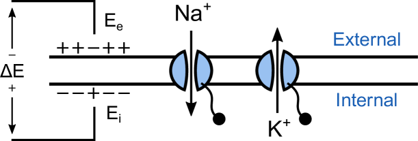
(a) Schematic of interacting ion channels

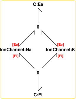
(b) Interacting Ion Channels

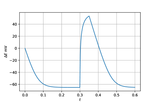
(c) Action potential $\Delta E$

Figure 3: Coupled Na+ and K+ ion channels motivated by the Hodgkin-Huxley model of the squid giant axon^{35, 18}. (a) A schematic of a Na+ channel and K+ channel located on the same charged membrane. (b) A model of this membrane can be created by coupling together two instances of the ion channel module (IonChannel) of Figure 2(c); one instance corresponds to the Na+ channel (IonChannel:Na) and one to K+ channel (IonChannel:K). The electrical components C:$\mathbf{Ee}$ and C:$\mathbf{Ei}$, corresponding to the external and internal membrane voltages $E_{e}$ and $E_{i}$ within the ion channel module, become the ports [Ee] and [Ei]. The 0 junctions ensure that the external and internal membrane voltages $E_{e}$ and $E_{i}$ are shared with the corresponding ion channel voltages. (c) Action potential. Concentrations (mM) are taken from Table 2.1 of Keener and Sneyd ²⁰: External. $c_{Na}=$437\text{\,}\mathrm{m}\mathrm{M}$$, $c_{K}=$20\text{\,}\mathrm{m}\mathrm{M}$$; Internal. $c_{Na}=$50\text{\,}\mathrm{m}\mathrm{M}$$, $c_{K}=$397\text{\,}\mathrm{m}\mathrm{M}$$ and correspond to the model of Hodgkin and Huxley ³⁵.

A strength of the graphical nature of the bond graph approach is that individual modules can be duplicated and connected. In this example, two instances of the ion channel module (Figure 2(c)) are combined in Figure 3(b) to model the action potential (Figure 3(a)). The species concentrations are encapsulated in the individual modules, but the electrical C components are shared via the ports. This is a simplified version of the Hodgkin-Huxley³⁵ model of the squid giant axon and the corresponding Na+ and K+ concentrations are used.

In the Hodgkin and Huxley ³⁵ model and in reality, the gating variables are dynamically modulated by the membrane potential $\Delta E$. However, for simplicity, we model the gating variables as externally controlled variables in this example. Accordingly, gating variables $G_{Na}$ and $G_{K}$ are piecewise constant functions of time:

$$G_{K} =\begin{cases}10^{-6}&\text{for $0.3<t<0.35$}\\ 1&\text{otherwise}\end{cases}$$ (16)

$$G_{Na} =\begin{cases}1&\text{for $0.3<t<0.35$}\\ 4.3\times 10^{-3}&\text{otherwise}\end{cases}$$ (17)

The time course of the membrane potential $\Delta E$ is shown in Figure 3(c) and can be explained as follows:

$t<0.3$: $\Delta E$ moves from the initial condition of zero to a resting potential of about $-65$mV. This corresponds to the value in Table 2.1 of Keener and Sneyd ²⁰; the resting potential depends not only on Nernst potentials of Na+ and K+ but also on the values of the gating potential (i.e. their relative permeability).

$0.3<t<0.35$: The Na+ gate opens, causing the membrane potential $\Delta E$ to move towards the Nernst potential for Na+. This results in the initial depolarisation phase of the action potential.

$t>0.35$ The Na+ gate closes and the K+ gate opens, causing $\Delta E$ to return to the resting potential. This completes the repolarisation phase of the action potential.

Redox Reactions and Proton Pumps

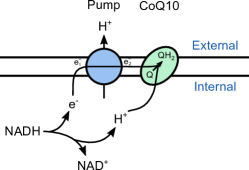
(a) Redox reaction schematic

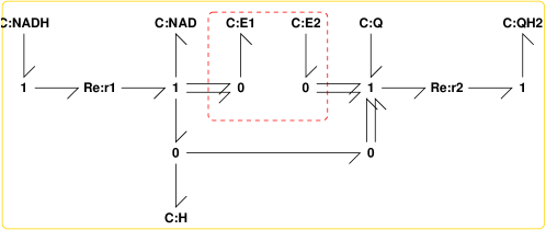
(b) Redox reaction

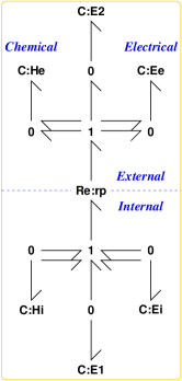
(c) Proton Pump

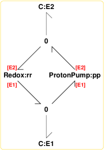
(d) Complex I

Figure 4: Redox Reactions and Proton Pump. (a) A schematic of the redox reaction and proton pump. The electrons generated from the redox reaction ($\text{e}_{1}^{-}$) are shuttled through the proton pump to pump hydrogen into the intermembrane space. Following this, the electron ($\text{e}_{2}^{-}$) is then delivered to Coenzyme Q10. (b) A bond graph of the redox reaction. Half-reactions (Redox Reactions and Proton Pumps) and (Redox Reactions and Proton Pumps) are represented by the reaction components Re:$\mathbf{r1}$ and Re:$\mathbf{r2}$ respectively. The dashed box corresponds to the electrical part of the bond graph with C:$\mathbf{E1}$ and C:$\mathbf{E2}$ representing the accumulations of electrons e1- and e2-. The double bonds correspond to a stoichiometry of 2. (c) Bond graph of the proton pump. Re:$\mathbf{rp}$ corresponds to reaction (LABEL:eq:PP). Internal and external protons H_i^+and H_e^+ have chemical properties represented by C:$\mathbf{Hi}$ and C:$\mathbf{He}$ respectively and electrical properties represented by C:$\mathbf{Ei}$ and C:$\mathbf{Ee}$ respectively. The redox potential difference $E_{1}-E_{2}$ drives the protons across the membrane. (d) Bond graph of the redox reaction and proton pump coupled together.

In his book Power, Sex, Suicide: Mitochondria and the Meaning of Life³⁶, Nick Lane points towards the fundamental role that redox reactions play in biology, stating that “essentially all of the energy-generating reactions of life are redox reactions”. One such energy-generating reaction that within the mitochondrial respiratory chain is

$$\ch{NADH+Q+H+<>[r]NAD++QH2}$$ (18)

As noted by Nicholls and Ferguson ²², “The additional facility afforded by an electrochemical treatment of a redox reaction is the ability to dissect the overall electron transfer into two half-reactions involving the donation and acceptance of electrons respectively”. With this in mind, reaction (18) can be divided into the reactions:

A bond graph representation of this decomposition is given in Figure 4(b).

Species	$\phi^{\ominus}~{}($\mathrm{mV}$)$19	Conc.	$\phi~{}($\mathrm{mV}$)$
NAD	188	5.02e-0437	-15
NADH	407	7.50e-0537	154
Q	675	1.00e-0238	552
QH2	-241	1.00e-0238	-365
H	0	1.00e-07	-431

Table 3: Faraday-equivalent potentials with $pH=7$ and equal concentrations of Q and QH2. The potentials $\phi$ are computed from Equation (6).

From the bond graph, the reaction potentials of the two half-reactions are:

$$\Phi_{1} =\phi_{\ch{NADH}}-\left(2E_{1}+\phi_{\ch{H}}+\phi_{\ch{NAD}}\right)$$ (25)

$$\Phi_{2} =2E_{2}+2\phi_{\ch{H}}+\phi_{\ch{Q}}-\phi_{\ch{QH2}}$$ (26)

where $E_{1}$ and $E_{2}$ are the potentials associated the electrical capacitors C:$\mathbf{E1}$ and C:$\mathbf{E2}$ and the associated electrons e1- and e2-. At equilibrium $\Phi_{1}=\Phi_{2}=0$. Hence, using the values in Table 3, the voltages corresponding to the capacitors C:$\mathbf{E1}$ and C:$\mathbf{E2}$ are

$$E_{1} =\frac{1}{2}\left(154+15+431\right)=$300\text{\,}\mathrm{mV}$$$ (27)

$$E_{2} =\frac{1}{2}\left(-365-552+2\times 431\right)=$-28\text{\,}\mathrm{mV}$$$ (28)

Hence the net electronic potential $\Delta\mathcal{E}=E_{1}-E_{2}=$328\text{\,}\mathrm{mV}$$ is available to power a proton pump (note the distinction from the membrane potential $\Delta E=E_{i}-E_{e}$ in earlier sections). Indeed, reaction (18) occurs within complex I of the mitochondrial respiratory chain (Figure 4(a)). Complex I is a “giant molecular proton pump”³⁹ which uses the high-energy electron ($\ch{e1-}$) from Reaction (Redox Reactions and Proton Pumps) to generate a proton gradient across the mitochondrial membrane before the lower-energy electron ($\ch{e2-}$) is consumed by Reaction (Redox Reactions and Proton Pumps).

In this case, two protons are pumped across the membrane for each electron. Such an electron-driven proton pump can be modelled by the bond graph of Figure 4(c); the corresponding equation is

The reaction affinity is

$$\Phi_{rp}=\Delta\mathcal{E}-\Delta p$$ (29)

where we have defined the proton-motive force $\Delta p$ to be the sum of the electrical and chemical potentials arising from the proton (H+) gradient across the membrane ²²:

$$\Delta p=\phi_{e}-\phi_{i}-\Delta E$$ (30)

where $\phi_{e}$ and $\phi_{i}$ are the chemical potentials of the external and internal protons $H_{e}^{+}$ and $H_{i}^{+}$. At equilibrium, $\Phi_{rp}=0$ and it follows that

$$\Delta p =\frac{\Delta\mathcal{E}}{2}=$164\text{\,}\mathrm{mV}$$$ (31)

The PMF of Equation (31) corresponds to the equilibrium value with standard concentrations of the species in Table 3. This value will change if the concentrations of the species change or due to potential losses in the Re components when the flows are non zero. In fact the exchange of species between complexes CI, CIII and CIV, in particular Q and QH2, leads to an “affinity equalisation” of PMFs between the three complexes with a typical PMF of approximately $230\text{\,}\mathrm{mV}$ ¹⁹.

Example: Sodium-Glucose Symporter

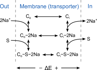
(a) Reaction network

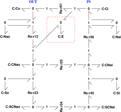
(b) Bond graph

Figure 5: Sodium-Glucose Symporter. (a) A schematic of the reaction network of the transporter. Under physiological conditions, the symporter uses the natural inward electrochemical gradient of Na^+ to drive transport of the sugar glucose (S) into the cell, against a chemical gradient. The transporter operates via a six-state mechanism (outer loop), with a leakage reaction that causes Na^+ to be translocated without coupling to the transport of glucose. (b) A bond graph of the transpoter. The cycle formed by the reactions in the outer loop (Re:$\mathbf{r12}$, Re:$\mathbf{r23}$, Re:$\mathbf{r34}$, Re:$\mathbf{r45}$, Re:$\mathbf{r56}$ and Re:$\mathbf{r61}$) is driven by the outside and inside concentrations of sodium (C:$\mathbf{Nao}$ and C:$\mathbf{Nai}$ respectively) and glucose (C:$\mathbf{So}$ and C:$\mathbf{Si}$). Re:$\mathbf{r25}$ represents the leakage reaction. The contribution of the membrane potential is given by the C:$\mathbf{E}$ component in the dashed red box.

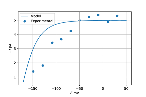
Figure 6: Theoretical and experimental results. The experimental results of Eskandari et al. ⁴⁰ are compared with the bond graph model with the parameters of Tables 4 and 5 and total number of transporters $N_{C}=7.5\times 10^{7}$.

The transport of substrates across a membrane is vital to cellular homeostasis. It is widely acknowledged that the laws of thermodynamics constrain the direction of flux through a transporter; a thermodynamic treatment is given in Hill ⁴¹ and a bond graph approaches are developed in Gawthrop and Crampin ⁴² and Pan et al. ⁴³. In the case of electrogenic transporters that translocates a net charge across a membrane, the effects of membrane potential must be considered. This section looks at a particular electrogenic transporter: the Sodium-Glucose Transport Protein 1 (SGLT1) (also known as the Na+/glucose symporter) which was studied experimentally and explained by a biophysical model ^{40, 44, 45, 46}. When operating normally, sugar is transported from the outside to the inside of the membrane driven against a possibly adverse gradient by the concentration gradient of Na+ (Figure 5(a)).

According to Parent et al. ⁴⁵, p.64, “The carrier is assumed to bear a charge $z=-2$ with the result that the Na+ loaded carrier is electroneutral.” Hence, in terms of Figure 5(b), the two complexes corresponding to C:$\mathbf{Ci}$ and C:$\mathbf{Co}$ bear a charge of $-2$ whereas the loaded complexes C:$\mathbf{CNao}$, C:$\mathbf{SCNao}$, C:$\mathbf{SCNai}$ and C:$\mathbf{CNai}$ are electrically neutral.

With reference to the bond graph of Figure 5(b), the only reactions with electrogenic properties are those corresponding to: Re:$\mathbf{r61}$ where the unloaded complex passes from the inside to the outside of the membrane; Re:$\mathbf{r12}$ where the external Na+ of C:$\mathbf{CNao}$ binds/unbinds to the complex and Re:$\mathbf{r56}$ where the internal Na+ of C:$\mathbf{CNai}$ binds/unbinds to the complex. As discussed by Parent et al. ⁴⁵ their experimental results suggest the “absence of voltage dependence for internal Na+ binding, and thus asymmetrical binding sites at the external and internal face of the membrane.” In the context of the bond graph model of Figure 5(b), this implies that the reaction corresponding to Re:$\mathbf{r56}$ is not electrogenic and thus electrogenic effects are confined to the reactions corresponding to Re:$\mathbf{r61}$ and Re:$\mathbf{r12}$. These considerations give rise to Figure 5(b) where the portion within the dashed box corresponds to electrogenic effects. A non-electrogenic version of this model is analysed in § 1.1 of Hill ⁴¹ and in Gawthrop and Crampin ⁴².

Parameters

Reac.	$k_{f}$	$k_{r}$	$k_{eq}=\frac{k_{f}}{k_{r}}$	$\kappa$
r12	80000	500	160	10.1796
r23	100000	20	5000	202.023
r34	50	50	1	505.058
r45	800	12190	0.0656276	8080.93
r56	10	4500	0.00222222	67.1184
r61	3	350	0.00857143	8.67804
r25	0.3	0.00091	329.67	0.00610777

Table 4: Reaction Parameters

Species	$\phi^{\ominus}$ (mV)
So	61.71
Si	61.84
Nao	70.42
Nai	70.36
Co	98.76
CNao	104.03
SCNao	-61.78
Ci	-28.37
CNai	-50.86
SCNai	-61.78

Table 5: Species Parameters, referenced to a standard concentration of 1 M for the substrates (So, Si, Nao, Nai) and to a standard amount of 1 mol for transporter states (Co, CNao, SCNao, Ci, CNai, SCNai)

As is common in the literature, the experimentally derived reaction parameters are expressed in terms of forward $k_{f}$ and reverse $k_{r}$ rate constants whereas bond graph models are parameterised in terms of the standard potential $\phi^{\ominus}$ (3) and reaction rate constant $\kappa$ (8). Thus these parameters need to be converted into equivalent bond graph parameters. The thermodynamically consistent reaction kinetic parameters listed in the first two columns of Table 4 (given in Figure 6B of Eskandari et al. ⁴⁰), and are converted into ten equivalent thermodynamic constants using the methods described in Gawthrop and Crampin ⁴².

The total number of transporters $N_{C}$ per unit area corresponding to the experimental situation reported by Eskandari et al. ⁴⁰ is a key parameter. It not only determines the steady state flows but also the transient time constants; here it is adjusted to fit the data shown in Figure 6. The fitted theoretical results are compared with experimental values in Figure 6.

No model is definitive but rather is a step towards understanding a system and suggesting further experiments. For example, the model presented here assumes that the transmembrane current is entirely due to tranlocated charge. Charge leakage could be included as an ohmic resistance associated with the electrical C:$\mathbf{E}$ component and the corresponding resistance fitted to the model. As well as potentially allowing a better fit to the data, such a refined model would suggest further experimental verification.

The inhibition of the Na+/glucose symporter has been suggested as a treatment for type 2 diabetes mellitus ⁴⁷. It is hoped that physically based models, such as that developed here, will eventually lead to computational approaches to understanding such diseases and evaluating treatment strategies.

Conclusion

The study of bioelectrical systems can be greatly facilitated by a modelling framework that is both graphical and physically consistent. In this perspective, a series of examples has illustrated how Network Thermodynamics, as implemented with bond graphs, provides a graphical framework for modelling bioelectrical systems while ensuring thermodynamic consistency. This is made possible by treating electricity and chemistry in a unified fashion where potentials and flows are given in the same electrical units.

The method is naturally modular and any C component within a system can be used as a port to connect to other subsystems. This provides a flexible hierarchical approach to creating large models of bioelectrical systems. Moreover, the use of energy ports allows one particular model of a subsystem to be replaced by another with the same ports, allowing one to swap submodels within a large model to allow high detail in one part whilst simplifying the rest. This approach is made possible by the fact that even low-resolution submodels are thermodynamically consistent; for example it is possible to build a low resolution but physically plausible model of the mitochondrial electron transport chain ²⁵.

Energy flow in the form of molecules, protons and electrons shapes cell evolution ^{48, 49}; in the same vein, energy is central to synthetic biology  ^{50, 51, 52, 53}. Hence it is appropriate to use the energy-based modelling approach to bioelectricity to not only evaluate natural systems from an evolutionary point of view but also to evaluate novel bioelectrical approaches to synthetic biology such as, for example, the generation of electricity from waste and making microbial communities form specific patterns ⁵⁴.

A set of Python-based tools https://pypi.org/project/BondGraphTools/ is available to assist model building ⁵⁵ and to provide avenues for the automation of model development.

References

- Schofield et al. 2020 Zoe Schofield, Gabriel N. Meloni, Peter Tran, Christian Zerfass, Giovanni Sena, Yoshikatsu Hayashi, Murray Grant, Sonia A. Contera, Shelley D. Minteer, Minsu Kim, Arthur Prindle, Paulo Rocha, Mustafa B. A. Djamgoz, Teuta Pilizota, Patrick R. Unwin, Munehiro Asally, and Orkun S. Soyer. Bioelectrical understanding and engineering of cell biology. Journal of The Royal Society Interface, 17(166):20200013, 2020. doi: 10.1098/rsif.2020.0013.
- Zerfaß et al. 2019 Christian Zerfaß, Munehiro Asally, and Orkun S. Soyer. Interrogating metabolism as an electron flow system. Current Opinion in Systems Biology, 13:59 – 67, 2019. ISSN 2452-3100. doi: 10.1016/j.coisb.2018.10.001. • Systems biology of model organisms • Systems ecology and evolution.
- Djamgoz et al. 2014 Mustafa B. A. Djamgoz, R. Charles Coombes, and Albrecht Schwab. Ion transport and cancer: from initiation to metastasis. Philosophical Transactions of the Royal Society B: Biological Sciences, 369(1638):20130092, 2014. doi: 10.1098/rstb.2013.0092.
- Pchelintseva and Djamgoz 2018 Ekaterina Pchelintseva and Mustafa B. A. Djamgoz. Mesenchymal stem cell differentiation: Control by calcium-activated potassium channels. Journal of Cellular Physiology, 233(5):3755–3768, 2018. doi: 10.1002/jcp.26120.
- Young et al. 2020 Cameron C. Young, Armin Vedadghavami, and Ambika G. Bajpayee. Bioelectricity for drug delivery: The promise of cationic therapeutics. Bioelectricity, 2(2):68–81, 2020. doi: 10.1089/bioe.2020.0012.
- Anwar et al. 2019 Muhammad Anwar, Sulin Lou, Liu Chen, Hui Li, and Zhangli Hu. Recent advancement and strategy on bio-hydrogen production from photosynthetic microalgae. Bioresource Technology, 292, 2019. ISSN 0960-8524. doi: 10.1016/j.biortech.2019.121972.
- Gaffney et al. 2020 Erin M Gaffney, Matteo Grattieri, Zayn Rhodes, and Shelley D Minteer. Exploration of computational approaches for understanding microbial electrochemical systems: Opportunities and future directions. Journal of The Electrochemical Society, 167(6), 2020. doi: 10.1149/1945-7111/ab872e.
- Gleizer et al. 2020 Shmuel Gleizer, Yinon M. Bar-On, Roee Ben-Nissan, and Ron Milo. Engineering microbes to produce fuel, commodities, and food from CO2. Cell Reports Physical Science, 1(10):100223, 2020. ISSN 2666-3864. doi: 10.1016/j.xcrp.2020.100223.
- Pietak and Levin 2016 Alexis Pietak and Michael Levin. Exploring instructive physiological signaling with the bioelectric tissue simulation engine. Frontiers in Bioengineering and Biotechnology, 4:55, 2016. ISSN 2296-4185. doi: 10.3389/fbioe.2016.00055.
- Paynter 1961 H. M. Paynter. Analysis and Design of Engineering Systems. MIT Press, Cambridge, Mass., 1961.
- Gawthrop and Smith 1996 P. J. Gawthrop and L. P. S. Smith. Metamodelling: Bond Graphs and Dynamic Systems. Prentice Hall, Hemel Hempstead, Herts, England., 1996. ISBN 0-13-489824-9.
- Gawthrop and Bevan 2007 Peter J Gawthrop and Geraint P Bevan. Bond-graph modeling: A tutorial introduction for control engineers. IEEE Control Systems Magazine, 27(2):24–45, April 2007. doi: 10.1109/MCS.2007.338279.
- Karnopp et al. 2012 Dean C Karnopp, Donald L Margolis, and Ronald C Rosenberg. System Dynamics: Modeling, Simulation, and Control of Mechatronic Systems. John Wiley & Sons, 5th edition, 2012. ISBN 978-0470889084.
- Oster et al. 1971 George Oster, Alan Perelson, and Aharon Katchalsky. Network thermodynamics. Nature, 234:393–399, December 1971. doi: 10.1038/234393a0.
- Oster et al. 1973 George F. Oster, Alan S. Perelson, and Aharon Katchalsky. Network thermodynamics: dynamic modelling of biophysical systems. Quarterly Reviews of Biophysics, 6(01):1–134, 1973. doi: 10.1017/S0033583500000081.
- Perelson 1975 A.S. Perelson. Network thermodynamics. an overview. Biophysical Journal, 15(7):667 – 685, 1975. ISSN 0006-3495. doi: 10.1016/S0006-3495(75)85847-4.
- Maxwell 1871 James Clerk Maxwell. Remarks on the mathematical classification of physical quantities. Proceedings London Mathematical Society, pages 224–233, 1871.
- Gawthrop et al. 2017 P. J. Gawthrop, I. Siekmann, T. Kameneva, S. Saha, M. R. Ibbotson, and E. J. Crampin. Bond graph modelling of chemoelectrical energy transduction. IET Systems Biology, 11(5):127–138, 2017. ISSN 1751-8849. doi: 10.1049/iet-syb.2017.0006. Available at arXiv:1512.00956.
- Gawthrop 2017 P. J. Gawthrop. Bond graph modeling of chemiosmotic biomolecular energy transduction. IEEE Transactions on NanoBioscience, 16(3):177–188, April 2017. ISSN 1536-1241. doi: 10.1109/TNB.2017.2674683. Available at arXiv:1611.04264.
- Keener and Sneyd 2009 James P Keener and James Sneyd. Mathematical Physiology: I: Cellular Physiology, volume 1. Springer, New York, 2nd edition, 2009.
- Rudy and Silva 2006 Yoram Rudy and Jonathan R. Silva. Computational biology in the study of cardiac ion channels and cell electrophysiology. Quarterly Reviews of Biophysics, 39(1):57–116, 2006. doi: 10.1017/S0033583506004227.
- Nicholls and Ferguson 2013 David G Nicholls and Stuart Ferguson. Bioenergetics 4. Academic Press, Amsterdam, 2013.
- Gawthrop and Crampin 2016 P. J. Gawthrop and E. J. Crampin. Modular bond-graph modelling and analysis of biomolecular systems. IET Systems Biology, 10(5):187–201, October 2016. ISSN 1751-8849. doi: 10.1049/iet-syb.2015.0083. Available at arXiv:1511.06482.
- Hunter 2016 Peter Hunter. The virtual physiological human: The physiome project aims to develop reproducible, multiscale models for clinical practice. IEEE Pulse, 7(4):36–42, July 2016. ISSN 2154-2287. doi: 10.1109/MPUL.2016.2563841.
- Gawthrop et al. 2020 Peter J. Gawthrop, Peter Cudmore, and Edmund J. Crampin. Physically-plausible modelling of biomolecular systems: A simplified, energy-based model of the mitochondrial electron transport chain. Journal of Theoretical Biology, 493:110223, 2020. ISSN 0022-5193. doi: 10.1016/j.jtbi.2020.110223.
- Paynter 1993 Henry M. Paynter. Preface. In J. J. Granda and F. E. Cellier, editors, Proceedings of the International Conference On Bond Graph Modeling (ICBGM’93), volume 25 of Simulation Series, page v, La Jolla, California, U.S.A., January 1993. Society for Computer Simulation. ISBN 1-56555-019-6.
- Gawthrop and Crampin 2014 Peter J. Gawthrop and Edmund J. Crampin. Energy-based analysis of biochemical cycles using bond graphs. Proceedings of the Royal Society A: Mathematical, Physical and Engineering Science, 470(2171):1–25, 2014. doi: 10.1098/rspa.2014.0459. Available at arXiv:1406.2447.
- Polettini and Esposito 2014 Matteo Polettini and Massimiliano Esposito. Irreversible thermodynamics of open chemical networks. I. Emergent cycles and broken conservation laws. The Journal of Chemical Physics, 141(2):024117, 2014. doi: 10.1063/1.4886396.
- Gawthrop and Crampin 2018 P. Gawthrop and E. J. Crampin. Bond graph representation of chemical reaction networks. IEEE Transactions on NanoBioscience, 17(4):449–455, October 2018. ISSN 1536-1241. doi: 10.1109/TNB.2018.2876391. Available at arXiv:1809.00449.
- Gawthrop et al. 2015 Peter J. Gawthrop, Joseph Cursons, and Edmund J. Crampin. Hierarchical bond graph modelling of biochemical networks. Proceedings of the Royal Society A: Mathematical, Physical and Engineering Sciences, 471(2184):1–23, 2015. ISSN 1364-5021. doi: 10.1098/rspa.2015.0642. Available at arXiv:1503.01814.
- Van Rysselberghe 1958 Pierre Van Rysselberghe. Reaction rates and affinities. The Journal of Chemical Physics, 29(3):640–642, 1958. doi: 10.1063/1.1744552.
- Sterratt et al. 2011 David Sterratt, Bruce Graham, Andrew Gillies, and David Willshaw. Principles of Computational Modelling in Neuroscience. Cambridge University Press, 2011. ISBN 9780521877954.
- Hille 2001 Bertil Hille. Ion Channels of Excitable Membranes. Sinauer Associates, Sunderland, MA, USA, 3rd edition, 2001. ISBN 978-0-87893-321-1.
- Pan et al. 2018 Michael Pan, Peter J. Gawthrop, Kenneth Tran, Joseph Cursons, and Edmund J. Crampin. Bond graph modelling of the cardiac action potential: implications for drift and non-unique steady states. Proceedings of the Royal Society of London A: Mathematical, Physical and Engineering Sciences, 474(2214), 2018. ISSN 1364-5021. doi: 10.1098/rspa.2018.0106. Available at arXiv:1802.04548.
- Hodgkin and Huxley 1952 A. L. Hodgkin and A. F. Huxley. A quantitative description of membrane current and its application to conduction and excitation in nerve. The Journal of Physiology, 117(4):500–544, 1952.
- Lane 2018 Nick Lane. Power, Sex, Suicide: Mitochondria and the meaning of life. Oxford University Press, Oxford, 2nd edition, 2018.
- Park et al. 2016 Junyoung O. Park, Sara A. Rubin, Yi-Fan Xu, Daniel Amador-Noguez, Jing Fan, Tomer Shlomi, and Joshua D. Rabinowitz. Metabolite concentrations, fluxes and free energies imply efficient enzyme usage. Nat Chem Biol, 12(7):482–489, Jul 2016. ISSN 1552-4450. doi: 10.1038/nchembio.2077.
- Bazil et al. 2016 Jason N. Bazil, Daniel A. Beard, and Kalyan C. Vinnakota. Catalytic coupling of oxidative phosphorylation, ATP demand, and reactive oxygen species generation. Biophysical Journal, 110(4):962 – 971, 2016. ISSN 0006-3495. doi: 10.1016/j.bpj.2015.09.036.
- Sazanov 2015 Leonid A. Sazanov. A giant molecular proton pump: structure and mechanism of respiratory complex I. Nat Rev Mol Cell Biol, 16(6):375–388, Jun 2015. ISSN 1471-0072. URL http://dx.doi.org/10.1038/nrm3997.
- Eskandari et al. 2005 S. Eskandari, E. M. Wright, and D. D. F. Loo. Kinetics of the Reverse Mode of the Na+/Glucose Cotransporter. J Membr Biol, 204(1):23–32, Mar 2005. ISSN 0022-2631. doi: 10.1007/s00232-005-0743-x. 16007500[pmid].
- Hill 1989 Terrell L Hill. Free energy transduction and biochemical cycle kinetics. Springer-Verlag, New York, 1989.
- Gawthrop and Crampin 2017 Peter J. Gawthrop and Edmund J. Crampin. Energy-based analysis of biomolecular pathways. Proceedings of the Royal Society of London A: Mathematical, Physical and Engineering Sciences, 473(2202), 2017. ISSN 1364-5021. doi: 10.1098/rspa.2016.0825. Available at arXiv:1611.02332.
- Pan et al. 2019 Michael Pan, Peter J. Gawthrop, Kenneth Tran, Joseph Cursons, and Edmund J. Crampin. A thermodynamic framework for modelling membrane transporters. Journal of Theoretical Biology, 481:10 – 23, 2019. ISSN 0022-5193. doi: 10.1016/j.jtbi.2018.09.034. Available at arXiv:1806.04341.
- Parent et al. 1992a Lucie Parent, Stéphane Supplisson, Donald D. F. Loo, and Ernest M. Wright. Electrogenic properties of the cloned Na+/glucose cotransporter: I. voltage-clamp studies. The Journal of Membrane Biology, 125(1):49–62, 1992a. ISSN 1432-1424. doi: 10.1007/BF00235797.
- Parent et al. 1992b Lucie Parent, Stéphane Supplisson, Donald D. F. Loo, and Ernest M. Wright. Electrogenic properties of the cloned Na+/glucose cotransporter: II. a transport model under nonrapid equilibrium conditions. The Journal of Membrane Biology, 125(1):63–79, 1992b. ISSN 1432-1424. doi: 10.1007/BF00235798.
- Chen et al. 1995 Xing-Zhen Chen, Michael J Coady, Francis Jackson, Alfred Berteloot, and Jean-Yves Lapointe. Thermodynamic determination of the Na+: glucose coupling ratio for the human SGLT1 cotransporter. Biophysical Journal, 69(6):2405, 1995. doi: 10.1016/S0006-3495(95)80110-4.
- Scheen 2020 André J Scheen. Sodium–glucose cotransporter type 2 inhibitors for the treatment of type 2 diabetes mellitus. Nature Reviews Endocrinology, pages 1–22, 2020.
- Lane and Martin 2010 Nick Lane and William Martin. The energetics of genome complexity. Nature, 467(7318):929–934, Oct 2010. ISSN 0028-0836. doi: 10.1038/nature09486.
- Lane 2020 Nick Lane. How energy flow shapes cell evolution. Current Biology, 30(10):R471 – R476, 2020. ISSN 0960-9822. doi: 10.1016/j.cub.2020.03.055.
- Zerfaß et al. 2018 Christian Zerfaß, Jing Chen, and Orkun S Soyer. Engineering microbial communities using thermodynamic principles and electrical interfaces. Current Opinion in Biotechnology, 50:121 – 127, 2018. ISSN 0958-1669. doi: 10.1016/j.copbio.2017.12.004. Energy biotechnology • Environmental biotechnology.
- Berhanu et al. 2019 Samuel Berhanu, Takuya Ueda, and Yutetsu Kuruma. Artificial photosynthetic cell producing energy for protein synthesis. Nature Communications, 10(1):1325, 2019. ISSN 2041-1723. doi: 10.1038/s41467-019-09147-4. URL https://doi.org/10.1038/s41467-019-09147-4.
- Delattre et al. 2020 Hadrien Delattre, Jing Chen, Matthew J. Wade, and Orkun S. Soyer. Thermodynamic modelling of synthetic communities predicts minimum free energy requirements for sulfate reduction and methanogenesis. Journal of The Royal Society Interface, 17(166):20200053, 2020. doi: 10.1098/rsif.2020.0053.
- Roell and Zurbriggen 2020 Marc-Sven Roell and Matias D Zurbriggen. The impact of synthetic biology for future agriculture and nutrition. Current Opinion in Biotechnology, 61:102 – 109, 2020. ISSN 0958-1669. doi: 10.1016/j.copbio.2019.10.004.
- Bradley 2019 Robert Bradley. Bio-electrical engineering: a promising frontier for synthetic biology. The Biochemist, 41(3):10–13, 06 2019. ISSN 0954-982X. doi: 10.1042/BIO04103010.
- Cudmore et al. 2019 Peter Cudmore, Peter J. Gawthrop, Michael Pan, and Edmund J. Crampin. Computer-aided modelling of complex physical systems with BondGraphTools. Available at arXiv:1906.10799, Jun 2019.