Technical Report: The Policy Graph Improvement Algorithm

Joni Pajarinen J.ย Pajarinen is with Aalto University, Finland and Intelligent Autonomous Systems lab, TU Darmstadt, Germany joni.pajarinen@aalto.fi
Abstract

Optimizing a partially observable Markov decision process (POMDP) policy is challenging. The policy graph improvement (PGI) algorithm for POMDPs represents the policy as a fixed size policy graph and improves the policy monotonically. Due to the fixed policy size, computation time for each improvement iteration is known in advance. Moreover, the method allows for compact understandable policies. This report describes the technical details of the PGIย [1] and particle based PGIย [2] algorithms for POMDPs in a more accessible way than [1] or [2] allowing practitioners and students to understand and implement the algorithms.

I POMDP

In a POMDP, the agent operates in a world defined by the current state s๐‘ s. However, the agent does not observe s๐‘ s directly but makes indirect observations about the state of the world. At each time step $t$, the agent executes an action $a$, receives a reward Rโ€‹(s,a)๐‘…๐‘ ๐‘ŽR(s,a), and the world transitions to a new state sโ€ฒsuperscript๐‘ โ€ฒs^{\prime} with probability Pโ€‹(sโ€ฒ|s,a)๐‘ƒconditionalsuperscript๐‘ โ€ฒ๐‘ ๐‘ŽP(s^{\prime}|s,a). The agent makes then an observation $o$ with probability Pโ€‹(o|sโ€ฒ,a)๐‘ƒconditional๐‘œsuperscript๐‘ โ€ฒ๐‘ŽP(o|s^{\prime},a). In a POMDP, the agent can make optimal decisions based on the complete action-observation history or a probability distribution over states. The goal of the agent is to choose actions which maximize the expected total reward Eโ€‹[โˆ‘t=0Tโˆ’1Rโ€‹(sโ€‹(t),aโ€‹(t))|ฯ€,b0]๐ธdelimited-[]conditionalsuperscriptsubscript๐‘ก0๐‘‡1๐‘…๐‘ ๐‘ก๐‘Ž๐‘ก๐œ‹subscript๐‘0E[\sum_{t=0}^{T-1}R(s(t),a(t))|\pi,b_{0}] over $T$ time steps, where $\pi$ is the policy and $b_{0}$ is the belief, the initial probability distribution over states.

II Policy graph improvement (PGI) algorithm

The PGI algorithm [1, Algorithm 1] improves the value, that is, the expected total reward over T๐‘‡T time steps, of a fixed size POMDP policy graph (and Dec-POMDP policy graphs) 
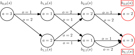
monotonically. The policy graph is an acyclic graph that consists of T๐‘‡T layers of nodes. A policy graph node executes an action and an edge, for each possible observation, defines the next node to
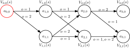
 transition to. Figureย 1 shows an example of a policy graph. See the figure caption for a discussion on how the agent uses the policy graph for choosing actions.

Figure 1: Example policy graph. The policy graph consists of layers of nodes. Each layer corresponds to one time step. Execution starts at the far left and proceeds to the right. The agent executes actions specified by the policy graph. At time step $t$: 1) the agent executes action $a_{t,q}$ in policy graph layer $t$, where $q$ is the index of the current policy graph node, 2) depending on the current world state and action, the agent receives a reward and the world transitions to a new state, 3) the agent makes an observation $o$ about the new world state, 4) the execution moves to the next policy graph node $q^{\prime}$ in the next layer $t+1$ along the edge with the matching observation, 5) in the next time step $t+1$ the agent executes action $a_{t+1,q^{\prime}}$ and so on.

PGI shares some properties with point based POMDP methods which apply value iteration with piece wise linear convex (PWLC) value functions represented as a set of alpha vectors [3]. Essentially, PGI contains an alpha vector at each graph node but it differs from standard PWLC methods in that it 1) restricts the number of alpha vectors at each time step, 2) restricts alpha vectors to specific time steps and allows only alpha vector backups from the next time step, 3) generates a completely new set of beliefs after changing the policy. PGI shares the high level idea of alternating between a forward and backward pass with methods such as differential dynamic programming (DDP) https://en.wikipedia.org/wiki/Differential_dynamic_programming.

II-A Notation

$t$ denotes current time step. $q$ denotes the index of a policy graph node. $t,q$ denotes graph node $q$ at time step $t$. $A$ is the set of actions and $a\in A$ is one action. $O$ denotes the set of observations and $o\in O$ denotes a single observation. $S$ is the set of states and sโˆˆS๐‘ ๐‘†s\in S is a single state. sโ€ฒsuperscript๐‘ โ€ฒs^{\prime} denotes the next time step state and $q^{\prime}$ denotes the next time step policy graph node.

Pโ€‹(o,sโ€ฒ|s,a)=Pโ€‹(sโ€ฒ|s,a)โ€‹Pโ€‹(o|sโ€ฒ,a)๐‘ƒ๐‘œconditionalsuperscript๐‘ โ€ฒ๐‘ ๐‘Ž๐‘ƒconditionalsuperscript๐‘ โ€ฒ๐‘ ๐‘Ž๐‘ƒconditional๐‘œsuperscript๐‘ โ€ฒ๐‘ŽP(o,s^{\prime}|s,a)=P(s^{\prime}|s,a)P(o|s^{\prime},a) is the joint transition and observation probability. bt,qโ€‹(s)subscript๐‘๐‘ก๐‘ž๐‘ b_{t,q}(s) is the non-normalized belief at time step $t$ at policy graph node $q$. $b$ denotes beliefs at all policy graph nodes.

$\pi$ denotes policy. $\pi$ consists of $P_{t}(a|q)$ and $P_{t}(q^{\prime}|q,o)$. $P_{t}(a|q)$ denotes the probability to execute action $a$ at time step $t$ at policy graph node $q$. $P_{t}(q^{\prime}|q,o)$ denotes probability to move to policy graph node $q^{\prime}$ after observing $o$ in policy graph node $q$ at time step $t$. Note that in the PGI algorithm $P_{t}(a|q)$ and $P_{t}(q^{\prime}|q,o)$ are deterministic. Because of the deterministic policy we often denote the action at time step $t$ and at node $q$ with $a_{t,q}$ and the best mapping from action $a$, observation $o$, current node $q$ to next node as $q_{t+1}(a,o,q)$.

II-B PGI for POMDPs

Algorithmย 1 defines PGI for POMDPs (without policy
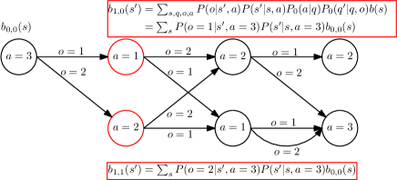
 compressionย [1]). Figureย 2 illustrates the forward pass which projects the initial belief, using the current policy, from the first time step to the last
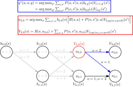
 one. Figureย 3 illustrates the dynamic programming back pass which optimizes the policy graph for the projected beliefs starting from the last layer and proceeding to the first one.

Policy compression. Policy compressionย [1] recomputes policies for โ€œredundantโ€ nodes which get an identical policy as another policy graph node in the same layer/time step and, as such, are not useful. A new policy can be computed for the redundant node using a random belief.

1 $\pi$ = PGI(b0โ€‹(s)subscript๐‘0๐‘ b_{0}(s), $\pi_{0}$)
ย ย ย ย ย  Input: Initial belief b0โ€‹(s)subscript๐‘0๐‘ b_{0}(s), initial policy $\pi_{0}=[P_{0}(a|q),P_{0}(q^{\prime}|q,o)]$
ย ย ย ย ย  Output: Optimized policy $\pi$
2ย ย ย ย ย  whileย No convergence and time limit not exceededย do
3ย ย ย ย ย ย ย ย ย ย  b=๐‘absentb=ForwardPass(b0โ€‹(s)subscript๐‘0๐‘ b_{0}(s), $\pi$)
4ย ย ย ย ย ย ย ย ย ย  ฯ€=๐œ‹absent\pi=BackPass($b$)
5ย ย ย ย ย ย ย ย ย ย  end while
6ย ย ย ย ย ย ย ย ย ย 
7ย ย ย ย ย ย ย ย ย ย 
Algorithmย 1 Monotonic policy graph improvement (PGI) algorithm for POMDPs
1
2$b=$ForwardPass(b0โ€‹(s)subscript๐‘0๐‘ b_{0}(s), $\pi$)
3ย ย ย ย ย  b0,0โ€‹(s)=b0โ€‹(s)subscript๐‘00๐‘ subscript๐‘0๐‘ b_{0,0}(s)=b_{0}(s)
4ย ย ย ย ย  forย Time step $t=0$ to $T-1$ย do
5ย ย ย ย ย ย ย ย ย ย  foreachย Policy graph node $q^{\prime}$ at layer $t+1$ย do
6ย ย ย ย ย ย ย ย ย ย ย ย ย ย ย  bt+1,qโ€ฒโ€‹(sโ€ฒ)=โˆ‘q,o,a,sPโ€‹(o,sโ€ฒ|s,a)โ€‹Ptโ€‹(a|q)โ€‹Ptโ€‹(qโ€ฒ|q,o)โ€‹bt,qโ€‹(s)subscript๐‘๐‘ก1superscript๐‘žโ€ฒsuperscript๐‘ โ€ฒsubscript๐‘ž๐‘œ๐‘Ž๐‘ ๐‘ƒ๐‘œconditionalsuperscript๐‘ โ€ฒ๐‘ ๐‘Žsubscript๐‘ƒ๐‘กconditional๐‘Ž๐‘žsubscript๐‘ƒ๐‘กconditionalsuperscript๐‘žโ€ฒ๐‘ž๐‘œsubscript๐‘๐‘ก๐‘ž๐‘ b_{t+1,q^{\prime}}(s^{\prime})=\sum_{q,o,a,s}P(o,s^{\prime}|s,a)P_{t}(a|q)P_{t}(q^{\prime}|q,o)b_{t,q}(s)
7ย ย ย ย ย ย ย ย ย ย ย ย ย ย ย  end foreach
8ย ย ย ย ย ย ย ย ย ย ย ย ย ย ย 
9ย ย ย ย ย ย ย ย ย ย ย ย ย ย ย  end for
10ย ย ย ย ย ย ย ย ย ย ย ย ย ย ย 
11ย ย ย ย ย ย ย ย ย ย ย ย ย ย ย 
Algorithmย 2 PGI forward pass
1
2$\pi=$BackPass($b$)
3ย ย ย ย ย  VT+1โ€‹(s)=0subscript๐‘‰๐‘‡1๐‘ 0V_{T+1}(s)=0
4ย ย ย ย ย  forย Time step $t=T$ to 00ย do
5ย ย ย ย ย ย ย ย ย ย  foreachย Policy graph node $q$ at layer $t$ย do
6ย ย ย ย ย ย ย ย ย ย ย ย ย ย ย  // Best next layer graph node $q_{t+1}$
7ย ย ย ย ย ย ย ย ย ย ย ย ย ย ย  // for $(a,o,q)$:
8ย ย ย ย ย ย ย ย ย ย ย ย ย ย ย  qt+1โ€‹(a,o,q)=argmaxqโ€ฒโ€‹โˆ‘s,sโ€ฒPโ€‹(o,sโ€ฒ|s,a)โ€‹bt,qโ€‹(s)โ€‹Vt+1,qโ€ฒโ€‹(sโ€ฒ)subscript๐‘ž๐‘ก1๐‘Ž๐‘œ๐‘žsubscriptargmaxsuperscript๐‘žโ€ฒsubscript๐‘ superscript๐‘ โ€ฒ๐‘ƒ๐‘œconditionalsuperscript๐‘ โ€ฒ๐‘ ๐‘Žsubscript๐‘๐‘ก๐‘ž๐‘ subscript๐‘‰๐‘ก1superscript๐‘žโ€ฒsuperscript๐‘ โ€ฒq_{t+1}(a,o,q)=\operatornamewithlimits{argmax}_{q^{\prime}}\sum_{s,s^{\prime}}P(o,s^{\prime}|s,a)b_{t,q}(s)V_{t+1,q^{\prime}}(s^{\prime})
9ย ย ย ย ย ย ย ย ย ย ย ย ย ย ย  // Best action $a_{t,q}^{*}$ at node $q$:
10ย ย ย ย ย ย ย ย ย ย ย ย ย ย ย  at,qโˆ—=argmaxa[โˆ‘sbt,qโ€‹(s)โ€‹Rโ€‹(s,a)+โˆ‘s,sโ€ฒ,obt,qโ€‹(s)โ€‹Pโ€‹(o,sโ€ฒ|s,a)โ€‹Vt+1,qt+1โ€‹(a,o,q)โ€‹(sโ€ฒ)]subscriptsuperscript๐‘Ž๐‘ก๐‘žsubscriptargmax๐‘Žsubscript๐‘ subscript๐‘๐‘ก๐‘ž๐‘ ๐‘…๐‘ ๐‘Žsubscript๐‘ superscript๐‘ โ€ฒ๐‘œsubscript๐‘๐‘ก๐‘ž๐‘ ๐‘ƒ๐‘œconditionalsuperscript๐‘ โ€ฒ๐‘ ๐‘Žsubscript๐‘‰๐‘ก1subscript๐‘ž๐‘ก1๐‘Ž๐‘œ๐‘žsuperscript๐‘ โ€ฒa^{*}_{t,q}=\operatornamewithlimits{argmax}_{a}\Big{[}\sum_{s}b_{t,q}(s)R(s,a)+\sum_{s,s^{\prime},o}b_{t,q}(s)P(o,s^{\prime}|s,a)V_{t+1,q_{t+1}(a,o,q)}(s^{\prime})\Big{]}
11ย ย ย ย ย ย ย ย ย ย ย ย ย ย ย  Ptโ€‹(a=at,qโˆ—|q)=1subscript๐‘ƒ๐‘ก๐‘Žconditionalsubscriptsuperscript๐‘Ž๐‘ก๐‘ž๐‘ž1P_{t}(a=a^{*}_{t,q}|q)=1
12ย ย ย ย ย ย ย ย ย ย ย ย ย ย ย  // Use $a^{*}_{t,q}$ to get next graph node:
13ย ย ย ย ย ย ย ย ย ย ย ย ย ย ย  Ptโ€‹(qโ€ฒ=qt+1โ€‹(at,qโˆ—,o,q)|q,o)=1subscript๐‘ƒ๐‘กsuperscript๐‘žโ€ฒconditionalsubscript๐‘ž๐‘ก1subscriptsuperscript๐‘Ž๐‘ก๐‘ž๐‘œ๐‘ž๐‘ž๐‘œ1P_{t}(q^{\prime}=q_{t+1}(a^{*}_{t,q},o,q)|q,o)=1
14ย ย ย ย ย ย ย ย ย ย ย ย ย ย ย  // Update value function at node $q$:
15ย ย ย ย ย ย ย ย ย ย ย ย ย ย ย 
Vt,qโ€‹(s)=subscript๐‘‰๐‘ก๐‘ž๐‘ absent\displaystyle V_{t,q}(s)= $\displaystyle\sum_{a}P_{t}(a|q)\Big{[}R(s,a)+\sum_{s^{\prime},o,q^{\prime}}$
$\displaystyle P(s^{\prime},o|s,a)P_{t}(q^{\prime}|q,o)V_{t+1,q^{\prime}}(s^{\prime})\Big{]}$
16ย ย ย ย ย ย ย ย ย ย ย ย ย ย ย  end foreach
17ย ย ย ย ย ย ย ย ย ย ย ย ย ย ย 
18ย ย ย ย ย ย ย ย ย ย ย ย ย ย ย  end for
19ย ย ย ย ย ย ย ย ย ย ย ย ย ย ย 
20ย ย ย ย ย ย ย ย ย ย ย ย ย ย ย 
Algorithmย 3 PGI dynamic programming back pass
Refer to caption
Refer to caption
Refer to caption
Refer to caption
Refer to caption
Figure 2: Illustration of the forward pass procedure. The top figure shows a summary of the procedure: project initial belief b0โ€‹(s)subscript๐‘0๐‘ b_{0}(s) through the whole policy graph from left to right using the current policy. The following figures show an example of the initial belief and the projection steps.
Refer to caption
Refer to caption
Refer to caption
Refer to caption
Refer to caption
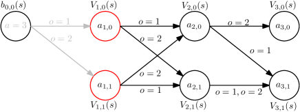
Figure 3: Illustration of the dynamic programming back pass. The top figure shows a summary of the procedure: start from the last policy graph layer on the right and update the policy and value function at each policy graph layer going from right to left. At each node compute best action and for each observation a forward edge based on the belief at the node. The following figures show an example of the backward pass.

II-C Particle PGI

Particle PGI (PPGI)ย [2] can compute policies for POMDPs with very large state spaces by using a particle based approximation of the belief and by approximating the value function by sampling. Other POMDP methods which use a particle representation include DESPOTย [4], POMCPย [5], and MCVIย [6]. One advantage of PPGI is a fixed size policy which is incrementally improved instead of growing the policy.

When using a particle based belief, the belief consists of a weighted set of particles: bโ€‹(s)=โˆ‘i=1Nwiโ€‹ฮดโ€‹(s,si);โˆ‘iwi=1;0โ‰คwiโ‰ค1formulae-sequence๐‘๐‘ superscriptsubscript๐‘–1๐‘subscript๐‘ค๐‘–๐›ฟ๐‘ subscript๐‘ ๐‘–formulae-sequencesubscript๐‘–subscript๐‘ค๐‘–10subscript๐‘ค๐‘–1b(s)=\sum_{i=1}^{N}w_{i}\delta(s,s_{i});\sum_{i}w_{i}=1;0\leq w_{i}\leq 1, where $w_{i}$ is the particle weight and ฮดโ€‹(s,si)๐›ฟ๐‘ subscript๐‘ ๐‘–\delta(s,s_{i}) is the delta function: ฮดโ€‹(s,si)=1๐›ฟ๐‘ subscript๐‘ ๐‘–1\delta(s,s_{i})=1 only when s=si๐‘ subscript๐‘ ๐‘–s=s_{i}, otherwise zero. Algorithmย 7 shows how to perform an approximate Bayesian belief update using particles for a belief given an action and observation.

$N_{t,q}$ denotes the number of particles in belief bt,qโ€‹(s)subscript๐‘๐‘ก๐‘ž๐‘ b_{t,q}(s). Algorithmย 4 shows the particle based forward pass. Algorithmย 5 shows the particle based backwards pass. Algorithmย 5 follows [6, Algorithm 1], and, hence, the approximation error bounds in [6] apply.

1
2$b=$ParticleForwardPass(b0โ€‹(s)subscript๐‘0๐‘ b_{0}(s), $\pi$)
3ย ย ย ย ย  b0,0โ€‹(s)=b0โ€‹(s)subscript๐‘00๐‘ subscript๐‘0๐‘ b_{0,0}(s)=b_{0}(s)
4ย ย ย ย ย  forย Time step $t=0$ to $T-1$ย do
5ย ย ย ย ย ย ย ย ย ย  Set bt+1,qโ€ฒโ€‹(sโ€ฒ)subscript๐‘๐‘ก1superscript๐‘žโ€ฒsuperscript๐‘ โ€ฒb_{t+1,q^{\prime}}(s^{\prime}) to an empty set for all $q^{\prime}$
6ย ย ย ย ย ย ย ย ย ย  foreachย Policy graph node $q$ at layer $t$ย do
7ย ย ย ย ย ย ย ย ย ย ย ย ย ย ย  forย i=1๐‘–1i=1 to $N_{t,q}$ย do
8ย ย ย ย ย ย ย ย ย ย ย ย ย ย ย ย ย ย ย ย  // Sample state sisubscript๐‘ ๐‘–s_{i}, next state siโ€ฒsuperscriptsubscript๐‘ ๐‘–โ€ฒs_{i}^{\prime},
9ย ย ย ย ย ย ย ย ย ย ย ย ย ย ย ย ย ย ย ย  // and observation $o_{i}$:
10ย ย ย ย ย ย ย ย ย ย ย ย ย ย ย ย ย ย ย ย  a=ฯ€โ€‹(q)๐‘Ž๐œ‹๐‘ža=\pi(q)
11ย ย ย ย ย ย ย ย ย ย ย ย ย ย ย ย ย ย ย ย  siโˆผbt,qโ€‹(s)similar-tosubscript๐‘ ๐‘–subscript๐‘๐‘ก๐‘ž๐‘ s_{i}\sim b_{t,q}(s)
12ย ย ย ย ย ย ย ย ย ย ย ย ย ย ย ย ย ย ย ย  siโ€ฒโˆผPโ€‹(sโ€ฒ|si,a)similar-tosuperscriptsubscript๐‘ ๐‘–โ€ฒ๐‘ƒconditionalsuperscript๐‘ โ€ฒsubscript๐‘ ๐‘–๐‘Žs_{i}^{\prime}\sim P(s^{\prime}|s_{i},a)
13ย ย ย ย ย ย ย ย ย ย ย ย ย ย ย ย ย ย ย ย  oiโˆผPโ€‹(o|siโ€ฒ,a)similar-tosubscript๐‘œ๐‘–๐‘ƒconditional๐‘œsuperscriptsubscript๐‘ ๐‘–โ€ฒ๐‘Žo_{i}\sim P(o|s_{i}^{\prime},a)
14ย ย ย ย ย ย ย ย ย ย ย ย ย ย ย ย ย ย ย ย  Add state siโ€ฒsuperscriptsubscript๐‘ ๐‘–โ€ฒs_{i}^{\prime} to bt+1,qt+1โ€‹(a,oi,q)โ€‹(sโ€ฒ)subscript๐‘๐‘ก1subscript๐‘ž๐‘ก1๐‘Žsubscript๐‘œ๐‘–๐‘žsuperscript๐‘ โ€ฒb_{t+1,q_{t+1}(a,o_{i},q)}(s^{\prime})
15ย ย ย ย ย ย ย ย ย ย ย ย ย ย ย ย ย ย ย ย  end for
16ย ย ย ย ย ย ย ย ย ย ย ย ย ย ย ย ย ย ย ย 
17ย ย ย ย ย ย ย ย ย ย ย ย ย ย ย ย ย ย ย ย  end foreach
18ย ย ย ย ย ย ย ย ย ย ย ย ย ย ย ย ย ย ย ย 
19ย ย ย ย ย ย ย ย ย ย ย ย ย ย ย ย ย ย ย ย  end for
20ย ย ย ย ย ย ย ย ย ย ย ย ย ย ย ย ย ย ย ย 
21ย ย ย ย ย ย ย ย ย ย ย ย ย ย ย ย ย ย ย ย 
Algorithmย 4 PPGI forward pass
1
2$\pi=$ParticleBackPass($b$)
3ย ย ย ย ย  forย Time step $t=T$ to 00ย do
4ย ย ย ย ย ย ย ย ย ย  foreachย Policy graph node $q$ at layer $t$ย do
5ย ย ย ย ย ย ย ย ย ย ย ย ย ย ย  foreachย Action $a$ย do
6ย ย ย ย ย ย ย ย ย ย ย ย ย ย ย ย ย ย ย ย  Ra=0subscript๐‘…๐‘Ž0R_{a}=0
7ย ย ย ย ย ย ย ย ย ย ย ย ย ย ย ย ย ย ย ย  Va,o,qโ€ฒ=0subscript๐‘‰๐‘Ž๐‘œsuperscript๐‘žโ€ฒ0V_{a,o,q^{\prime}}=0 for all $o$, $q^{\prime}$
8ย ย ย ย ย ย ย ย ย ย ย ย ย ย ย ย ย ย ย ย  Va,o=0subscript๐‘‰๐‘Ž๐‘œ0V_{a,o}=0 for all $o$
9ย ย ย ย ย ย ย ย ย ย ย ย ย ย ย ย ย ย ย ย  forย i=1๐‘–1i=1 to $N$ย do
10ย ย ย ย ย ย ย ย ย ย ย ย ย ย ย ย ย ย ย ย ย ย ย ย ย  // Sample state sisubscript๐‘ ๐‘–s_{i}, next state siโ€ฒsuperscriptsubscript๐‘ ๐‘–โ€ฒs_{i}^{\prime},
11ย ย ย ย ย ย ย ย ย ย ย ย ย ย ย ย ย ย ย ย ย ย ย ย ย  // and observation $o$:
12ย ย ย ย ย ย ย ย ย ย ย ย ย ย ย ย ย ย ย ย ย ย ย ย ย  siโˆผbt,qโ€‹(s)similar-tosubscript๐‘ ๐‘–subscript๐‘๐‘ก๐‘ž๐‘ s_{i}\sim b_{t,q}(s)
13ย ย ย ย ย ย ย ย ย ย ย ย ย ย ย ย ย ย ย ย ย ย ย ย ย  siโ€ฒโˆผPโ€‹(sโ€ฒ|si,a)similar-tosuperscriptsubscript๐‘ ๐‘–โ€ฒ๐‘ƒconditionalsuperscript๐‘ โ€ฒsubscript๐‘ ๐‘–๐‘Žs_{i}^{\prime}\sim P(s^{\prime}|s_{i},a)
14ย ย ย ย ย ย ย ย ย ย ย ย ย ย ย ย ย ย ย ย ย ย ย ย ย  oiโˆผPโ€‹(o|siโ€ฒ,a)similar-tosubscript๐‘œ๐‘–๐‘ƒconditional๐‘œsuperscriptsubscript๐‘ ๐‘–โ€ฒ๐‘Žo_{i}\sim P(o|s_{i}^{\prime},a)
15ย ย ย ย ย ย ย ย ย ย ย ย ย ย ย ย ย ย ย ย ย ย ย ย ย  // Update immediate reward
16ย ย ย ย ย ย ย ย ย ย ย ย ย ย ย ย ย ย ย ย ย ย ย ย ย  Ra=Ra+Rโ€‹(si,a)subscript๐‘…๐‘Žsubscript๐‘…๐‘Ž๐‘…subscript๐‘ ๐‘–๐‘ŽR_{a}=R_{a}+R(s_{i},a)
17ย ย ย ย ย ย ย ย ย ย ย ย ย ย ย ย ย ย ย ย ย ย ย ย ย  foreachย Next node $q^{\prime}$ย do
18ย ย ย ย ย ย ย ย ย ย ย ย ย ย ย ย ย ย ย ย ย ย ย ย ย ย ย ย ย ย  // Simulate future value of siโ€ฒsuperscriptsubscript๐‘ ๐‘–โ€ฒs_{i}^{\prime}
19ย ย ย ย ย ย ย ย ย ย ย ย ย ย ย ย ย ย ย ย ย ย ย ย ย ย ย ย ย ย  Va,oi,qโ€ฒ=Va,oi,qโ€ฒ+subscript๐‘‰๐‘Žsubscript๐‘œ๐‘–superscript๐‘žโ€ฒlimit-fromsubscript๐‘‰๐‘Žsubscript๐‘œ๐‘–superscript๐‘žโ€ฒV_{a,o_{i},q^{\prime}}=V_{a,o_{i},q^{\prime}}+ Simulate(siโ€ฒsuperscriptsubscript๐‘ ๐‘–โ€ฒs_{i}^{\prime},$t+1$,$q^{\prime}$,$\pi$)
20ย ย ย ย ย ย ย ย ย ย ย ย ย ย ย ย ย ย ย ย ย ย ย ย ย ย ย ย ย ย 
21ย ย ย ย ย ย ย ย ย ย ย ย ย ย ย ย ย ย ย ย ย ย ย ย ย ย ย ย ย ย  end foreach
22ย ย ย ย ย ย ย ย ย ย ย ย ย ย ย ย ย ย ย ย ย ย ย ย ย ย ย ย ย ย 
23ย ย ย ย ย ย ย ย ย ย ย ย ย ย ย ย ย ย ย ย ย ย ย ย ย ย ย ย ย ย  end for
24ย ย ย ย ย ย ย ย ย ย ย ย ย ย ย ย ย ย ย ย ย ย ย ย ย ย ย ย ย ย foreachย Observation $o$ย do
25ย ย ย ย ย ย ย ย ย ย ย ย ย ย ย ย ย ย ย ย ย ย ย ย ย ย ย ย ย ย ย ย ย ย ย  // Next layer node $q_{t+1}(a,o,q)$ for
26ย ย ย ย ย ย ย ย ย ย ย ย ย ย ย ย ย ย ย ย ย ย ย ย ย ย ย ย ย ย ย ย ย ย ย  // current node $q$ and each
27ย ย ย ย ย ย ย ย ย ย ย ย ย ย ย ย ย ย ย ย ย ย ย ย ย ย ย ย ย ย ย ย ย ย ย  // $a$, $o$ combination:
28ย ย ย ย ย ย ย ย ย ย ย ย ย ย ย ย ย ย ย ย ย ย ย ย ย ย ย ย ย ย ย ย ย ย ย  qt+1โ€‹(a,o,q)=argmaxqโ€ฒVa,o,qโ€ฒsubscript๐‘ž๐‘ก1๐‘Ž๐‘œ๐‘žsubscriptargmaxsuperscript๐‘žโ€ฒsubscript๐‘‰๐‘Ž๐‘œsuperscript๐‘žโ€ฒq_{t+1}(a,o,q)=\operatornamewithlimits{argmax}_{q^{\prime}}V_{a,o,q^{\prime}}
29ย ย ย ย ย ย ย ย ย ย ย ย ย ย ย ย ย ย ย ย ย ย ย ย ย ย ย ย ย ย ย ย ย ย ย  Va,o=Va,o,qt+1โ€‹(a,o,q)subscript๐‘‰๐‘Ž๐‘œsubscript๐‘‰๐‘Ž๐‘œsubscript๐‘ž๐‘ก1๐‘Ž๐‘œ๐‘žV_{a,o}=V_{a,o,q_{t+1}(a,o,q)}
30ย ย ย ย ย ย ย ย ย ย ย ย ย ย ย ย ย ย ย ย ย ย ย ย ย ย ย ย ย ย ย ย ย ย ย 
31ย ย ย ย ย ย ย ย ย ย ย ย ย ย ย ย ย ย ย ย ย ย ย ย ย ย ย ย ย ย ย ย ย ย ย  end foreach
32ย ย ย ย ย ย ย ย ย ย ย ย ย ย ย ย ย ย ย ย ย ย ย ย ย ย ย ย ย ย ย ย ย ย ย Va=(Ra+โˆ‘oVa,o)/Nsubscript๐‘‰๐‘Žsubscript๐‘…๐‘Žsubscript๐‘œsubscript๐‘‰๐‘Ž๐‘œ๐‘V_{a}=(R_{a}+\sum_{o}V_{a,o})/N
33ย ย ย ย ย ย ย ย ย ย ย ย ย ย ย ย ย ย ย ย ย ย ย ย ย ย ย ย ย ย ย ย ย ย ย 
34ย ย ย ย ย ย ย ย ย ย ย ย ย ย ย ย ย ย ย ย ย ย ย ย ย ย ย ย ย ย ย ย ย ย ย  end foreach
35ย ย ย ย ย ย ย ย ย ย ย ย ย ย ย ย ย ย ย ย ย ย ย ย ย ย ย ย ย ย ย ย ย ย ย // Optimized action for node at $t,q$:
36ย ย ย ย ย ย ย ย ย ย ย ย ย ย ย ย ย ย ย ย ย ย ย ย ย ย ย ย ย ย ย ย ย ย ย  at,q=argmaxaVasubscript๐‘Ž๐‘ก๐‘žsubscriptargmax๐‘Žsubscript๐‘‰๐‘Ža_{t,q}=\operatornamewithlimits{argmax}_{a}V_{a}
37ย ย ย ย ย ย ย ย ย ย ย ย ย ย ย ย ย ย ย ย ย ย ย ย ย ย ย ย ย ย ย ย ย ย ย 
38ย ย ย ย ย ย ย ย ย ย ย ย ย ย ย ย ย ย ย ย ย ย ย ย ย ย ย ย ย ย ย ย ย ย ย  end foreach
39ย ย ย ย ย ย ย ย ย ย ย ย ย ย ย ย ย ย ย ย ย ย ย ย ย ย ย ย ย ย ย ย ย ย ย 
40ย ย ย ย ย ย ย ย ย ย ย ย ย ย ย ย ย ย ย ย ย ย ย ย ย ย ย ย ย ย ย ย ย ย ย  end for
41ย ย ย ย ย ย ย ย ย ย ย ย ย ย ย ย ย ย ย ย ย ย ย ย ย ย ย ย ย ย ย ย ย ย ย 
42ย ย ย ย ย ย ย ย ย ย ย ย ย ย ย ย ย ย ย ย ย ย ย ย ย ย ย ย ย ย ย ย ย ย ย 
Algorithmย 5 PPGI dynamic programming back pass
1
2$V=$Simulate(sisubscript๐‘ ๐‘–s_{i}, $t$, $q$, $\pi$)
3ย ย ย ย ย  V=Rโ€‹(si,at,q)๐‘‰๐‘…subscript๐‘ ๐‘–subscript๐‘Ž๐‘ก๐‘žV=R(s_{i},a_{t,q})
4ย ย ย ย ย  forย Time step $t$ to $T-1$ย do
5ย ย ย ย ย ย ย ย ย ย  siโ€ฒโˆผPโ€‹(sโ€ฒ|si,at,q)similar-tosuperscriptsubscript๐‘ ๐‘–โ€ฒ๐‘ƒconditionalsuperscript๐‘ โ€ฒsubscript๐‘ ๐‘–subscript๐‘Ž๐‘ก๐‘žs_{i}^{\prime}\sim P(s^{\prime}|s_{i},a_{t,q})
6ย ย ย ย ย ย ย ย ย ย  oiโˆผPโ€‹(o|siโ€ฒ,at,q)similar-tosubscript๐‘œ๐‘–๐‘ƒconditional๐‘œsuperscriptsubscript๐‘ ๐‘–โ€ฒsubscript๐‘Ž๐‘ก๐‘žo_{i}\sim P(o|s_{i}^{\prime},a_{t,q})
7ย ย ย ย ย ย ย ย ย ย  qโ€ฒ=qt+1โ€‹(at,q,oi,q)superscript๐‘žโ€ฒsubscript๐‘ž๐‘ก1subscript๐‘Ž๐‘ก๐‘žsubscript๐‘œ๐‘–๐‘žq^{\prime}=q_{t+1}(a_{t,q},o_{i},q)
8ย ย ย ย ย ย ย ย ย ย  V=V+Rโ€‹(sโ€ฒ,at+1,qโ€ฒ)๐‘‰๐‘‰๐‘…superscript๐‘ โ€ฒsubscript๐‘Ž๐‘ก1superscript๐‘žโ€ฒV=V+R(s^{\prime},a_{t+1,q^{\prime}})
9ย ย ย ย ย ย ย ย ย ย  // Move policy node and state to next time step:
10ย ย ย ย ย ย ย ย ย ย  q=qโ€ฒ๐‘žsuperscript๐‘žโ€ฒq=q^{\prime}, si=siโ€ฒsubscript๐‘ ๐‘–superscriptsubscript๐‘ ๐‘–โ€ฒs_{i}=s_{i}^{\prime}
11ย ย ย ย ย ย ย ย ย ย 
12ย ย ย ย ย ย ย ย ย ย  end for
13ย ย ย ย ย ย ย ย ย ย 
14ย ย ย ย ย ย ย ย ย ย 
Algorithmย 6 Simulate future state value given policy
1 bโ€‹(sโ€ฒ)=๐‘superscript๐‘ โ€ฒabsentb(s^{\prime})=ParticleBeliefUpdate(bโ€‹(s)๐‘๐‘ b(s), $a$, $o$)
2ย ย ย ย ย  Set bโ€‹(sโ€ฒ)๐‘superscript๐‘ โ€ฒb(s^{\prime}) to an empty set
3ย ย ย ย ย  forย i=1๐‘–1i=1 to |bโ€‹(s)|๐‘๐‘ |b(s)|ย do
4ย ย ย ย ย ย ย ย ย ย  wi,si=biโ€‹(s)subscript๐‘ค๐‘–subscript๐‘ ๐‘–subscript๐‘๐‘–๐‘ w_{i},s_{i}=b_{i}(s)
5ย ย ย ย ย ย ย ย ย ย  siโ€ฒโˆผPโ€‹(sโ€ฒ|si,a)similar-tosuperscriptsubscript๐‘ ๐‘–โ€ฒ๐‘ƒconditionalsuperscript๐‘ โ€ฒsubscript๐‘ ๐‘–๐‘Žs_{i}^{\prime}\sim P(s^{\prime}|s_{i},a)
6ย ย ย ย ย ย ย ย ย ย  wiโ€ฒ=wiโ€‹Pโ€‹(o|siโ€ฒ,a)superscriptsubscript๐‘ค๐‘–โ€ฒsubscript๐‘ค๐‘–๐‘ƒconditional๐‘œsuperscriptsubscript๐‘ ๐‘–โ€ฒ๐‘Žw_{i}^{\prime}=w_{i}P(o|s_{i}^{\prime},a)
7ย ย ย ย ย ย ย ย ย ย  Add wiโ€ฒ,siโ€ฒsuperscriptsubscript๐‘ค๐‘–โ€ฒsuperscriptsubscript๐‘ ๐‘–โ€ฒw_{i}^{\prime},s_{i}^{\prime} to bโ€‹(sโ€ฒ)๐‘superscript๐‘ โ€ฒb(s^{\prime})
8ย ย ย ย ย ย ย ย ย ย 
9ย ย ย ย ย ย ย ย ย ย  end for
10ย ย ย ย ย ย ย ย ย ย Normalize bโ€‹(sโ€ฒ)๐‘superscript๐‘ โ€ฒb(s^{\prime})
11ย ย ย ย ย ย ย ย ย ย 
12ย ย ย ย ย ย ย ย ย ย 
Algorithmย 7 Particle belief update

References

  • [1] J.ย Pajarinen and J.ย Peltonen, โ€œPeriodic finite state controllers for efficient POMDP and DEC-POMDP planning,โ€ in Advances in Neural Information Processing Systems (NIPS), 2011, pp. 2636โ€“2644.
  • [2] J.ย Pajarinen and V.ย Kyrki, โ€œRobotic manipulation of multiple objects as a POMDP,โ€ Artificial Intelligence, 2017.
  • [3] G.ย Shani, J.ย Pineau, and R.ย Kaplow, โ€œA survey of point-based POMDP solvers,โ€ Autonomous Agents and Multi-Agent Systems, vol.ย 27, no.ย 1, pp. 1โ€“51, 2013.
  • [4] A.ย Somani, N.ย Ye, D.ย Hsu, and W.ย S. Lee, โ€œDESPOT: Online POMDP planning with regularization,โ€ in Advances in Neural Information Processing Systems (NIPS), 2013, pp. 1772โ€“1780.
  • [5] D.ย Silver and J.ย Veness, โ€œMonte-Carlo planning in large POMDPs,โ€ in Advances in Neural Information Processing Systems (NIPS), 2010, pp. 2164โ€“2172.
  • [6] H.ย Bai, D.ย Hsu, W.ย S. Lee, and V.ย A. Ngo, โ€œMonte Carlo value iteration for continuous-state POMDPs,โ€ in Algorithmic foundations of robotics IX.ย ย ย Springer, 2010, pp. 175โ€“191.