SSP-Net: Scalable Sequential Pyramid Networks
for Real-Time 3D Human Pose Regression

Abstract

In this paper we propose a highly scalable convolutional neural network, end-to-end trainable, for real-time 3D human pose regression from still RGB images. We call this approach the Scalable Sequential Pyramid Networks (SSP-Net) as it is trained with refined supervision at multiple scales in a sequential manner. Our network requires a single training procedure and is capable of producing its best predictions at 120 frames per second (FPS), or acceptable predictions at more than 200 FPS when cut at test time. We show that the proposed regression approach is invariant to the size of feature maps, allowing our method to perform multi-resolution intermediate supervisions and reaching results comparable to the state-of-the-art with very low resolution feature maps. We demonstrate the accuracy and the effectiveness of our method by providing extensive experiments on two of the most important publicly available datasets for 3D pose estimation, Human3.6M and MPI-INF-3DHP. Additionally, we provide relevant insights about our decisions on the network architecture and show its flexibility to meet the best precision-speed compromise.

1 Introduction

Predicting 3D human poses from monocular images is an important task that benefits several applications, from human understanding and action recognition [1] to human shape analysis and character control [2], among many others. As a consequence of its high relevance, 3D human pose estimation is a very active topic, also due to the several challenges involved, such as the complexity in the human body structure, the variations in the visual aspects from one person to another, and the possibility of one or more body parts being occluded in the images. To handle these challenging cases, multi-scale analysis is traditionally used to allow a multi-level scene understanding.

With the breakthrough of deep Convolutional Neural Networks (CNNs) [3] alongside consistent computational power increase, human pose estimation methods have shifted from classical approaches [4, 5] to deep architectures [6, 7]. Most of current deep learning approaches for 3D human pose estimation are based on an extension of the stacked hourglass model [8] where each body joint is associated with a volumetric heatmap (e.g., [9]) that corresponds to the probability density of the joint in the 3D space. These volumetric heatmaps have two main issues. First, the accuracy of the pose estimation is very sensitive to the resolution of the volumetric heatmap, since the precision of the prediction is directly related to the volume of space encoded by a single voxel of the heatmap. Second, as large volumetric heatmaps are preferred, these methods require large amounts of memory to store the activations. The combination of these two issues results in neural architectures that do not scale well, that is, they are either accurate but very slow or quick but inaccurate. Furthermore, a new model has to be trained specifically for the chosen trade-off between speed and accuracy.

In the light of the limitations of current methods, we propose a new neural architecture that solves the scalability issues, by regressing the pose in multiple scales in a sequential coarse-to-fine approach. We call this approach the Scalable Sequential Pyramid Networks (SSP-Net). With a single training procedure, the SSP-Net produces a full model with several refined prediction outputs that can be cut a test time to select the best accuracy vs speed trade off. The contribution of this paper is an extremely fast 3D human body pose estimation architecture that obtains state of the art results at over 100 FPS. We also show that our method is robust to the resolution of the model, as it is able to obtain subpixel accuracy, leading to competitive results even for $4\times 4$ pixels feature maps.

The rest of this paper is divided as follows. In the next section, we present a review of the related work. The architecture of the proposed network and the proposed regression method are presented in Section 3. In Section 4, we show the experimental evaluation of our method on 3D human pose estimation, providing intuitions on the proposed method based on a detailed ablation study. We conclude the paper in Section 5.

2 Related work

In this section, we review some of the recent methods most related to our work, which are divide into two groups: 3D human pose estimation and Multi-stage architectures for human pose estimation. We encourage readers to read the survey on 3D human pose estimation in [10] for a more detailed bibliographic review.

2.1 3D human pose estimation

Estimating the human body joints in 3D coordinates from monocular RGB images is a challenging problem with a vast bibliography available in the literature [11, 12, 13, 14, 15, 16]. Despite the fact that methods for 2D pose estimation are mainly based on detection [8, 17], 3D pose estimation is frequently handled as a regression problem [18, 19]. The main reason is due to the additional third dimension in 3D predictions, which significantly increases the required memory and computations, especially in detection based approaches, were the space is frequently represented by voxels [20]. On the other hand, regression methods handle the problem more efficiently, usually resulting in precise estimations with lower resolution [1].

A common approach for 3D human pose regression is to lift 3D coordinates from 2D predictions [21, 22]. Despite being robust to visual variations, lifting 3D poses from 2D points is an ill-defined problem, which can result in ambiguity. In that case, incoherent predictions are common, which requires a matching strategy between the estimated 3D poses and a structural model [7]. As an alternative, the body joints can be represented relative to their parent joints, requiring the prediction of the delta between two neighbour joints [23, 24]. This approach reduces the variance in the target space. However, it introduces an accumulative error propagated from the root joint to the body extremities.

Another problem related to 3D pose estimation is the lack of rich visual data. Since precise 3D annotations depend on expensive and complex Motion Capture (MoCap) systems, public datasets are usually collected in controlled environment with static and clean background, despite having few subjects. To alleviate this problem, Mehta et al. [25] proposed to first train a 2D model on data collected “in-the-wild” with 2D manual annotations, and then to use transfer learning to build a neural network that predicts 3D joint positions with respect to the root joint. Transfer learning is an useful but tricky technique. For that reason, in our approach, we decided to have a single training procedure that uses manually 2D annotated data in-the-wild simultaneously with high precise MoCap data.

2.2 Multi-stage architectures for human pose estimation

Multi-stage architectures have been widely used for human pose estimation, specially for the more established problem of 2D pose estimation [26], usually as sequential predictions [27] or by means of recurrent networks [28]. A common practice in previous methods is to regress heatmap representations corresponding to a map of scores for a given body joint. The refinement of such heatmaps is crucial for achieving good precision, as noted in [29]. Following this idea, Newell et al. [8] proposed the stacked hourglass architecture, which is essentially a sequence of U-nets, each one producing a new set of heatmaps that are refined by further hourglasses. Approaches based on heatmap estimation have two drawbacks: first, predicted heatmaps require an elevated resolution for acceptable precision, since the body joint coordinates are extracted in a post-processing stage based on the argument of the maximum a posteriori probability (MAP or argmax). The second limitation is the requirement for artificially generated ground truth heatmaps during training, since argmax is not differentiable. Contrarily, in our method we can have precise predictions with very low resolution feature maps, in addition to not requiring artificially generated ground truth.

On 3D scenarios, Zhou et al. [30] benefits from 2D heatmaps to guide 3D pose regression, introducing a weakly-supervised approach for lifting 3D predictions from 2D data, and Pavlakos et al. [20] extended the Staked Hourglass network to volumetric heatmaps prediction, on which the $z$ coordinate is encoded in the additional heatmap dimension. However, the method proposed in [20] suffers from the significant increase in the number of parameters and in the required memory to store all the intermediate values, due to the highly expensive volumetric heatmaps. This problem can be alleviated by the differentiable version of argmax [31, 1], also called integral regression in [9], but it remains dependent on a costly voxilized representation of the 3D space.

The method presented in this work differs from all previous approaches in several aspects. First, it departs from requiring volumetric representations by predicting pairs of heatmaps and depth maps. Second, differently from the stacked hourglass architecture, our method has intermediate supervision at different scales, providing different levels of semantic and resolution, which are all aggregated in a densely connected way for better predictions refinement. Third, after a single training procedure, our scalable network can be cut at different positions, providing a vast trade off for precision vs. speed. All these advantages result from the proposed architecture, as detailed next.

3 Scalable Sequential Pyramid Networks

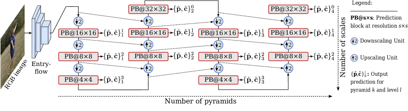
Figure 1: Global architecture of SSP-Net. The entry-flow extracts a preliminary feature map from the input image. These features are then fed through a sequence of CNNs composed of prediction blocks (PB) connected by alternating downscaling and upscaling units (DU and UU). Each PB outputs a supervised pose prediction that is refined by further blocks and units. See Figures 2 and 3 for the architectural details of DU, UU, and PB.

The proposed network architecture is depicted in Fig. 1. The input of our method is an RGB image $\mathbf{I}\in\mathbb{R}^{H\times{W}\times{3}}$ with resolution $H\times{W}$, which is feed to the entry flow network. The entry-flow produces convolutional features with resolution $\mathbb{R}^{H/4\times{W/4}\times{384}}$, which are then fed to a sequence of pyramids. The outputs of the network are a set of predicted 3D poses, designated by $\mathbf{p}_{k}^{l}\in\mathbb{R}^{{N}\times{3}}$, and optionally a set of joint confidence scores, designated by $\mathbf{c}_{k}^{l}\in\mathbb{R}^{{N}\times{1}}$, where $N$ is the number of body joints, $k$ is the pyramid index, and $l$ is the level index. All prediction blocks are supervised during training.

The motivation for a new architecture design is to provide an explicit multi-level supervision, enforcing the model to be able to represent the output independently on the resolution of feature maps. This approach allows the model to effectively combine low resolution feature maps, rich in semantic information, with high resolution features, containing more detailed information. In order to allow incrementally refined estimations, all predictions from both low and high resolutions are re-injected into the network. As a consequence of this densely supervised architecture, the network can offer early predictions with reduced computational time, or refined predictions with improved precision. The details about the proposed network are presented as follows.

Table 1: Entry-flow network.

	Layer	Filters	Size/strides	Output
	Input	$3$		$256\times 256$
	Convolution	$64$	$7\times 7/2$	$128\times 128$
	Convolution	$64$	$1\times 1$
	Convolution	$128$	$3\times 3$
	Residual			$128\times 128$
	MaxPooling		$3\times 3/2$	$64\times 64$
$2\times$	Convolution	$128$	$1\times 1$
	Convolution	$256$	$3\times 3$
	Residual			$64\times 64$
	MaxPooling		$2\times 2/2$	$32\times 32$
$2\times$	Convolution	$192$	$1\times 1$
	Convolution	$384$	$3\times 3$
	Residual			$32\times 32$

3.1 Network architecture

The global architecture of the proposed network (Fig. 1) is essentially composed of a combination of four modules: entry-flow, downscaling and upscaling units, and prediction blocks. The role of the entry-flow (detailed in Table 1) is to provide deep convolutional features extraction, which are successively downscaled and upscaled, respectively by downscaling and upscaling pyramids. Each pyramid is composed of a sequence of downscaling or upscaling units (DU or UU, see Fig. 2), interleaved with prediction blocks (PB) at each level. Prediction blocks are indexed by the pyramid index $k\in\{1,2,\dots,K\}$, where $K$ is the number of pyramids, and by the index level $l\in\{0,1,\dots,L\}$, where $L$ is the number of downscaling or upscaling steps performed, considering $k=1$ and $l=0$ the CNN features from the entry-flow. Note that in this arrangement, an odd $k$ index corresponds to a downscaling pyramid and an even $k$ index corresponds to an upscaling pyramid.

(a) Sep. residual block

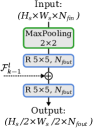
(b) Downscaling unit

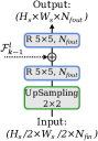
(c) Upscaling unit

Figure 2: Elementary blocks of the proposed network. In (a), the separable residual block which is used as the basic building block. In (b) and (c), the downscaling unit (DU) and upscaling unit (UU) take as secondary input the feature maps $\mathcal{F}_{k-1}^{l}$ issued from the previous pyramid. SC: (depthwise) separable convolution; R: separable residual block; $H_{s}\times{W_{s}}$: features size; $N_{fin/fout}$: number of input/output features.

The basic building block for the pyramid networks is the separable residual unit (Fig. 2(a)), which consists of a depth wise separable convolution [32] with a residual connection. Our choice for depth wise separable convolutions is mainly due to its benefits in efficiency [33]. One important advantage from our approach is the combination of features from different pyramids and levels. This is performed in both DU/UU, since they combine features from lower/higher levels, as well as features from previous pyramids.

Details of the prediction block (PB) are shown in Fig. 3. It takes as input a feature map $\mathcal{X}_{k}^{l}$, considering pyramid $k$ and level $l$, and produces a set of heatmaps $\mathbf{h}_{k}^{l}$ and depth maps $\mathbf{d}_{k}^{l}$, which are used for 3D pose regression (explained in Section 3.2). heatmaps and depth maps generation is defined in the following equations:

$$\mathcal{Y}_{k}^{l}=ReLU(BN(SC(\mathcal{X}_{k}^{l}))),$$ (1)

$$\mathbf{h}_{k}^{l}=\mathbf{W}_{h}^{k,l}\ast{\mathcal{Y}_{k}^{l}},$$ (2)

$$\mathbf{d}_{k}^{l}=\mathbf{W}_{d}^{k,l}\ast{\mathcal{Y}_{k}^{l}},$$ (3)

where $\mathcal{Y}_{k}^{l}$ is an intermediate feature representation, SC is a separable convolution, $\mathbf{W}_{h}^{k,l}$ and $\mathbf{W}_{d}^{k,l}$ are weight matrices with shape $\mathbb{R}^{N_{f}\times{N}}$, respectively for heatmaps and depth maps projection, and $\ast{}$ is the convolution operation. Additionally, each prediction block also produces a new feature map $\mathcal{F}_{k}^{l}$, which combines the input features with predicted heatmaps and depth maps, and is used by next blocks and units for further improvements. This step is defined in equation 4:

$$\mathcal{F}_{k}^{l}=\mathcal{X}_{k}^{l}+\mathcal{Y}_{k}^{l}\ +\mathbf{W}_{r}^{k,l}\ast{\mathbf{h}_{k}^{l}}\ +\mathbf{W}_{s}^{k,l}\ast{\mathbf{d}_{k}^{l}},$$ (4)

where $\mathbf{W}_{r}^{k,l}$ and $\mathbf{W}_{s}^{k,l}$ are called re-injection matrices.

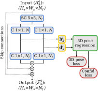
Figure 3: Network architecture of the prediction block. Input features $\mathcal{X}_{k}^{l}$ (for pyramid $k$ and level $l$) are used to produce heatmaps $\mathbf{h}_{k}^{l}$ and depth maps $\mathbf{d}_{k}^{l}$, from which 3D pose and confidence scores are estimated. Output features $\mathcal{F}_{k}^{l}$ are a combination of input features and re-injected predictions. C: convolution; SC: separable convolution; $H_{s}\times{W_{s}}$: features size; $N_{f}$: number of features; $N$: number of body joints.

Differently from the stacked hourglass [8, 20] architectures, where only the higher resolution features are supervised, we use intermediate supervision at every level of the pyramids. Adding more supervisions does not significantly increase the computational cost of our method, since contrarily to the stacked hourglass we do not need to generate artificial ground truth heatmaps. On the other hand, with intermediate supervisions in multiple levels we enforce the robustness of our method to variations in the scale of feature maps, while efficiently increasing the receptive field of the global network. Furthermore, our architecture injects the predictions from these intermediate supervisions back into the network by merging them with the current features. This allows the subsequent blocks to perform refining operations instead of full predictions.

3.2 3D pose regression approach

As discussed in Section 2, traditional regression methods use fully connected layers to learn a regression mapping from features to predictions. However, this approach usually gives sub-optimal solution. While methods in the state of the art are frequently based on detection, which requires expensive volumetric heatmap representations, regression approaches have the advantage of directly providing 3D pose prediction as joint coordinates without additional post-processing steps.

In our approach, we split the problem as 2D regression and depth estimation, using two different mappings: heatmaps for $(x,y)$ coordinates and depth maps for $z$. For 2D regression, we based our approach on the soft-argmax [31], and for depth estimation, we propose an new attention mechanism guided by 2D joint estimation. Our method does not require any parameter and is fully differentiable. The next sections explain each part of our approach.

3.2.1 Soft-argmax for 2D regression

Let us redefine the softmax operation on a single heatmap $\mathbf{h}\in\mathbb{R}^{H\times{W}}$ as:

$$\Phi(\mathbf{h})_{i,j}=\frac{e^{\mathbf{h}_{i,j}}}{\sum_{l=1}^{H}\sum_{c=1}^{W}e^{\mathbf{h}_{l,c}}},$$ (5)

where $\mathbf{h}_{i,j}$ is the value of $\mathbf{h}$ at location $(i,j)$ and $H\times{W}$ is the heatmap size. Contrary to the more common cross-channel softmax, we use here a spatial softmax to ensure that each heatmap is L1 normalized and positive. Then, we define the soft-argmax as:

$$\Psi_{d}(\mathbf{h})=\sum_{i=1}^{H}\sum_{j=1}^{W}\mathbf{W}_{i,j,d}\Phi(\mathbf{h})_{i,j},$$ (6)

where $\mathit{d}$ is a given component $\mathit{x}$ or $\mathit{y}$, and $\mathbf{W}$ is a $H\times{W}\times{2}$ weight matrix for both components $(x,y)$. The matrix $\mathbf{W}$ can be expressed by its components $\mathbf{W}_{x}$ and $\mathbf{W}_{y}$, which are 2D discrete normalized ramps, defined as follows:

$$\mathbf{W}_{i,j,x}=\frac{2j-1}{2W},\mathbf{W}_{i,j,y}=\frac{2i-1}{2H}.$$ (7)

Finally, given a heatmap $\mathbf{h}$, the regressed location in the image plane is given by:

$$\mathbf{\hat{p}}_{img}=(\Psi_{x}(\mathbf{h}),\Psi_{y}(\mathbf{h}))^{T}.$$ (8)

The soft-argmax operation can be seen as the 2D expectation of the normalized heatmap, which is a good approximation of the argmax function, considering that the exponential normalization results in a pointy distribution.

In order to integrate the soft-argmax layer into a deep neural network, we need its derivative with respect to $\mathbf{h}$:

$$\frac{\partial\Psi_{d}(\mathbf{h})}{\partial\mathbf{h}_{i,j}}=\mathbf{W}_{i,j,d}\Phi(\mathbf{h})_{i,j}(1-\Phi(\mathbf{h})_{i,j})-\sum_{l=1}^{H}\sum_{c=1}^{W}\mathbf{W}_{l,c,d}\Phi(\mathbf{h})_{i,j}\Phi(\mathbf{h})_{l,c}|_{l\neq{i};c\neq{j}}$$ (9)

The soft-argmax function can thus be integrated in a trainable framework by using back propagation and the chain rule on Equation 9. Moreover, similarly to what happens on softmax, the gradient is exponentially increasing for higher values, resulting in very discriminative response at the joint position.

The soft-argmax layer can be easily implemented in recent frameworks by concatenating a spatial softmax followed by one non-trainable convolutional layer with 2 filters of size $H\times{W}$, with fixed parameters according to Equation 7.

Unlike traditional argmax, soft-argmax provides sub-pixel accuracy, allowing good precision even with very low resolution. Additionally, our approach allows learning very discriminative heatmaps directly from the $(x,y)$ joint coordinates without explicitly computing artificial ground truth. Samples of heatmaps learned by our approach are shown in Fig. 7.

3.2.2 Joint based attention for depth estimation

For each body joint, we estimate its relative depth $\mathbf{\hat{z}}$ with respect to the root joint, which is usually designated by the pelvis. Specifically, we define an attention mechanism for predicted depth maps based on the appearance information encoded in heatmaps. Considering one heatmap $\mathbf{h}$ and the respective depth map $\mathbf{d}$, both with size $\mathbb{R}^{H\times{W}}$, the estimated relative depth is given by:

$$\mathbf{\hat{z}}=\frac{\sum_{i=1}^{H}\sum_{j=1}^{W}\mathbf{d}_{i,j}e^{\mathbf{h}_{i,j}}}{\sum_{i=1}^{H}\sum_{j=1}^{W}e^{\mathbf{h}_{i,j}}},$$ (10)

which can be interpreted as a selection of relevant regions from $\mathbf{d}$ based on the response from $\mathbf{h}$. In our implementation, values in depth maps are normalized in the interval $[0,1]$, corresponding to a range of depth prediction.

The 3D poses estimated by our approach are composed by the $(x,y)$ coordinates in pixels (Equation  8) and by the $z$ coordinate relative to the root joint. In order to recover the absolute 3D pose in world coordinates, we require the absolute depth of the root joint and the camera calibration parameters to convert pixels into millimeters. We believe that estimating the absolute 3D pose directly in world coordinates is not the most relevant problem, since the camera calibration can affect such a prediction drastically. On the other hand, the relative position of joints with respect to the root is of high relevance, and usually is the only measure used to compare different methods. We show in the experiments that absolute depth of the root joint can be estimated without major impact on accuracy.

3.2.3 Joint confidence score

Additionally to the joint locations, we estimate the joint confidence scores $\mathbf{\hat{c}}_{n}$, which corresponds to the probability of the $n^{th}$ joint being visible (or present, even if occluded) in the image. Given a normalized heatmap, any window with $2\times 2$ pixels is enough to regress a coordinate value with sub-pixel accuracy in a smaller squared region defined by the centers of the $2\times 2$ pixels, as depicted in Fig. 4. Therefore, we apply a summation with a $2\times 2$ sliding window on each normalized heatmap by using a SumPooling with stride 1, and take the maximum response as the confidence score. If the normalized heatmap is very pointy, the score is close to 1. On the other hand, if the normalized heatmap is smooth or has more than one separated region with high response, the confidence score drops.

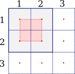
Figure 4: Estimation of joint confidence scores. The blue squares represent the pixels in the normalized heatmap with its center marked as a red dot. The red square is the region on which a coordinate can be regressed, considering responses only on the $2\times 2$ window from pixels (1, 1) to (2, 2).

Despite giving an additional piece of information, the joint confidence score does not depend on additional parameters and is computationally negligible, compared to the cost of the convolutional layers. Additionally, by supervising this output we can enforce the network to learn pointy responses for body parts.

4 Experiments

We evaluate the proposed method quantitatively on two challenging datasets for 3D human pose estimation: Human3.6M [34] and MPI-INF-3DHP [25]. We also use the manually annotated MPII Human Pose dataset (2D only) [35] to improve the quality of low level visual features of our network by mixing it with the other two datasets in a 50%/50% ratio on each training batch. Details about the 3D human pose datasets used in our experiments are provided as follows.

4.1 Datasets

Human3.6M Human3.6M [34] is a 3D human pose dataset composed of videos with 11 subjects performing 17 different activities, recorded by 4 cameras simultaneously, resulting in 3.6 million image frames. For each person, 17 joints are used in our method. The camera parameters are available, so it is possible to project the 3D joints to the image plane, as well as the inverse projection from points in the image plane plus depth back to world coordinates, where the error in computed in millimeters. On this dataset, we evaluate our method by measuring the mean per joint position error (MPJPE), which is a common metric used for this dataset. We followed the most common evaluation protocol [22, 23, 20, 25, 7] by taking five subjects for training (S1, S5, S6, S7, S8) and evaluating on two subjects (S9, S11) on one every 64th frames. On evaluation, the ground truth and the predicted poses are aligned on the root joint, and the error is computed on the remaining 16 joints. As in many similar approaches [22, 23, 20], we use ground truth person bounding boxes for image cropping and the absolute Z of the root joint to do the inverse projection. Nonetheless, we demonstrate in the ablation studies (Section 4.4) that errors in the absolute Z of the root joint are much less relevant than relative joint errors, and we also report our results using estimated absolute position.

MPI-INF-3DHP MPI-INF-3DHP [25] is, to the best of our knowledge, the most recent dataset for 3D human pose estimation. It was recorded with a markerless MoCap system, which allows videos to be recorded in outdoor environment e.g. , TS5 and TS6 from testing. A total of 8 actors were recorded performing 8 activities sets each. The activities involve some complex exercising poses, which makes this dataset more challenging than Human3.6M. The authors proposed three evaluation metrics: the mean per joint position error, in millimeters, the 3D Percentage of Correct Keypoints (PCK), and the Area Under the Curve (AUC) for different threshold on PCK. The standard threshold for PCK is 150mm. Differently from previous work, we use the real 3D poses to compute the error instead of the normalized 3D poses, since the last one cannot be easily computed from the image plane.

4.2 Implementation details

The proposed network was trained simultaneously on 3D pose regression and on joint confidence scores. For pose regression, we used the elastic net loss function (L1 + L2) [36]:

$$\mathcal{L}_{\mathbf{p}}=\frac{1}{N_{J}}\sum_{n=1}^{N_{J}}\|\mathbf{p}_{n}-\hat{\mathbf{p}}_{n}\|_{1}+\|\mathbf{p}_{n}-\hat{\mathbf{p}}_{n}\|_{2}^{2},$$ (11)

where $\mathbf{p}_{n}$ and $\hat{\mathbf{p}}_{n}$ are respectively the ground truth and the predicted $n^{th}$ joint coordinates. We use directly the joint coordinates normalized to the interval $[0,1]$, where the top-left image corner corresponds to $(0,0)$, and the bottom-right image corner corresponds to $(1,1)$. For the depth ($z$ coordinate), the root joint is assumed to have $z=0.5$, and a range of 2 meters is used to represent the remaining joints, which means that $z=0$ corresponds to a depth of $-1$ meter with respect to the root.

For the joint confidence scores, we use the binary cross entropy loss function:

$$\mathcal{L}_{\mathbf{c}}=\frac{1}{N_{J}}\sum_{n=1}^{N_{J}}[(\mathbf{c}_{n}-1)~{}log~{}(1-\hat{\mathbf{c}}_{n})-\mathbf{c}_{n}~{}log~{}\hat{\mathbf{c}}_{n}],$$ (12)

where $\mathbf{c}_{n}$ and $\hat{\mathbf{c}}_{n}$ are respectively the ground truth and the predicted confidence scores. We use $\mathbf{c}_{n}=1$ if the $n^{th}$ joint is present in the image and $\mathbf{c}_{n}=0$ otherwise.

The network architecture used in our experiments is implemented according to Fig. 1 and is composed of 8 pyramids, divided as 4 downscaling and 4 upscaling pyramids, each one with 4 scales ($K=8$ and $L=3$). We optimize the network using back propagation and RMSprop with batches of 24 images and initial learning rate of 0.001, which is divided by 10 when validation score plateaus. We used standard data augmentation on all datasets, including: random rotations ($\pm 30^{\circ}$), random bounding box rescaling with a factor from $0.7$ to $1.3$, and random brightness gain on color channels from $0.9$ to $1.1$.

4.3 Results on 3D pose estimation

Figure 5 shows some qualitative results of our method for 3D pose estimation, including challenging poses and some outdoor scenes. A quantitative evaluation is presented as follows.

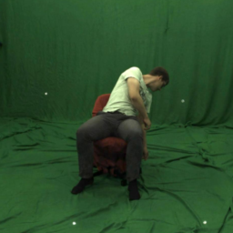
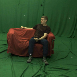
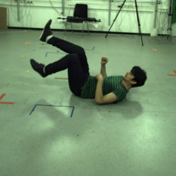
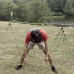
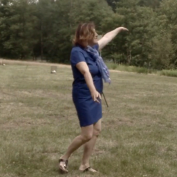
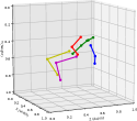
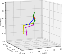
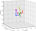
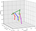
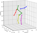
Figure 5: Input image samples (top), and their respective predicted 3D poses (bottom) for the MPI-INF-3DHP dataset, including two outdoor scenes (from testing).

Table 2: Comparison results with previous work on Human3.6M using the MPJPE (millimeters errors) evaluation on reconstructed poses. AZ: using the absolute $z$ of the root joint. MC: multi-crop, using 5 different bounding boxes with horizontal flip.

Methods	Dir.	Disc.	Eat	Greet	Phone	Posing	Purch.	Sit
Pavlakos et al. [20]	67.4	71.9	66.7	69.1	71.9	65.0	68.3	83.7
Mehta et al. [25]	52.5	63.8	55.4	62.3	71.8	52.6	72.2	86.2
Martinez et al. [22]	51.8	56.2	58.1	59.0	69.5	55.2	58.1	74.0
Luo et al. [24]∗	49.2	57.5	53.9	55.4	62.2	52.1	60.9	73.8
Sun et al. [23]	52.8	54.8	54.2	54.3	61.8	53.1	53.6	71.7
Luvizon et al. [1]	49.2	51.6	47.6	50.5	51.8	48.5	51.7	61.5
Sun et al. [9]	–	–	–	–	–	–	–	–
Ours 120 FPS	46.9	50.9	49.9	47.5	51.9	46.2	49.2	61.7
Ours +AZ	46.1	50.2	50.2	47.5	52.0	45.9	48.5	62.3
Ours +AZ+MC	45.1	49.1	49.0	46.5	50.6	44.8	47.7	60.6
Methods	SitD.	Smoke	Photo	Wait	Walk	WalkD.	WalkP.	Avg
Pavlakos et al. [20]	96.5	71.4	76.9	65.8	59.1	74.9	63.2	71.9
Mehta et al. [25]	120.0	66.0	79.8	63.9	48.9	76.8	53.7	68.6
Martinez et al. [22]	94.6	62.3	78.4	59.1	49.5	65.1	52.4	62.9
Luo et al. [24]$\star$	96.5	60.4	73.9	55.6	46.6	69.5	52.4	61.3
Sun et al. [23]	86.7	61.5	67.2	53.4	47.1	61.6	53.4	59.1
Luvizon et al. [1]	70.9	53.7	60.3	48.9	44.4	57.9	48.9	53.2
Sun et al. [9]	–	–	–	–	–	–	–	49.6
Ours 120 FPS	66.5	53.4	55.2	45.5	42.1	55.6	45.9	51.6
Ours +AZ	66.8	53.4	54.7	45.2	41.9	54.7	45.5	51.4
Ours +AZ+MC	65.4	52.0	52.8	44.2	40.6	54.1	44.4	50.2

^$\star$ Results using ground truth limb lengths.

4.3.1 Human3.6M

Table 2 shows our results compared to recent methods, where we achieve 50.2 mm average MPJPE considering multi-crop and 51.6 mm single-crop at 120 frames per second (FPS). Our approach achieves results comparable to the state-of-the-art overall, and improves individual activities up to 12.4% on “Photo” and 7.7% on “Sit down”, which is the most challenging case. In general, our method improves state-of-the-art on individual activities even on single-crop at full speed, running on a desktop GeForce GTX 1080Ti GPU, which is, to the best of our knowledge, better than any previous method. Additionally, with the proposed architecture, our approach can be even faster with a small decrease in performance, as shown in the ablation study.

We also evaluate our method using the estimated Z (depth) of root joints, which corresponds to our results when nothing else is specified. For doing that, we use a MLP with three layers and 128-128-256 neurons, which takes as input the image bounding box normalized coordinates (2D only) and a vector of visual features ($\mathcal{F}_{1}^{3}$), and outputs the estimated absolute Z of the root joint.

4.3.2 MPI-INF-3DHP

Our results on this dataset are presented in Table 3. We reached a comparable result to Luo et al. [24], Improving their result on the average PCK by 1.4%, while producing inferences much faster (120 FPS on a GTX 1080 Ti vs 20 FPS from [24] on a Titan XP). Furthermore, we are the only method to not use the universal normalized poses from this dataset, since our method requires the full pose in its original coordinates to allows camera projection.

Table 3: Comparison results with previous work on MPI-INF-3DHP using the PCK and AUC metrics (higher is better) and the MPJPE metric (lower is better), on reconstructed poses. AZ: using the absolute $z$ of the root joint.

Methods	Std. Walk	Exer.	Sit Chair	Croush Reach	OnThe Floor	Sport	Misc.	Avg
	PCK	PCK	PCK	PCK	PCK	PCK	PCK	PCK	AUC	MPJPE
Zhou et al. [30]$\star{}$	-	-	-	-	-	-	-	69.2	32.5	-
Mehta et al. [25]$\star{}$	86.6	75.3	74.8	73.7	52.2	82.1	77.5	75.7	39.3	117.6
Mehta et al. [6]$\star{}$	87.7	77.4	74.7	72.9	51.3	83.3	80.1	76.6	40.4	124.7
Luo et al. [24]$\star{}$	90.4	79.1	88.5	81.6	66.3	91.9	92.2	81.8	45.2	89.4
Ours +AZ	87.1	85.4	85.9	81.6	68.5	88.2	83.0	83.2	44.3	96.8

^$\star$ Results using the universal (normalized) ground truth poses.

4.4 Ablation study

In this section we provide some additional experiments that show the behaviour of our method with respect to the proposed network architecture.

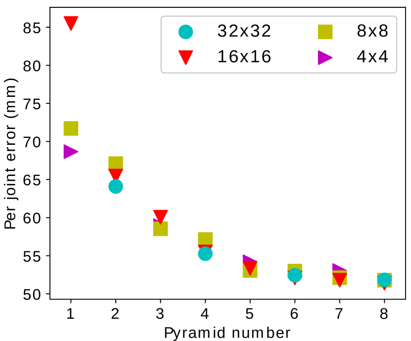
(a)

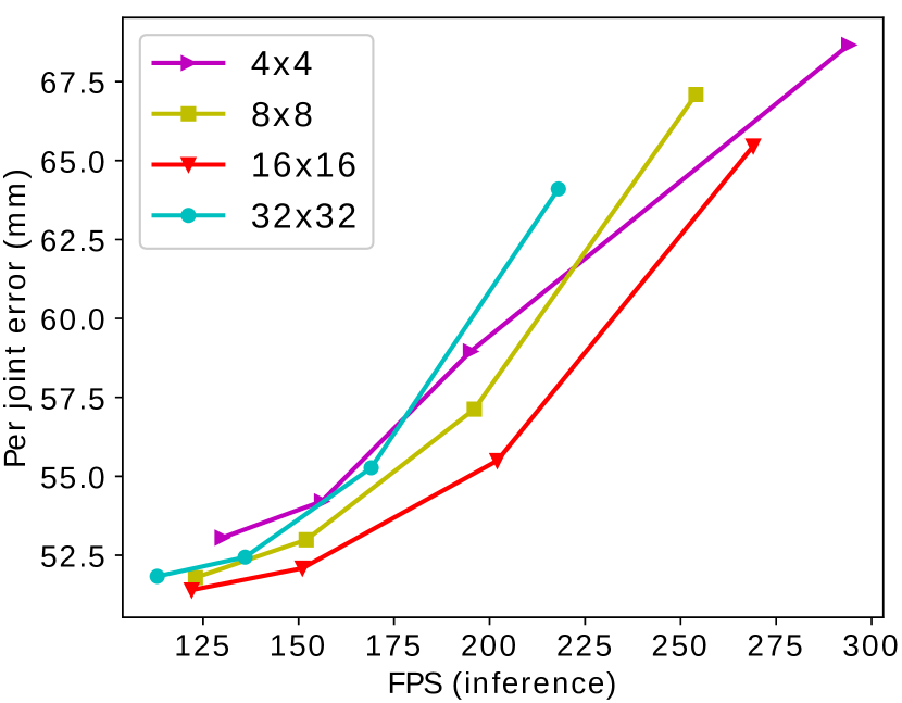
(b)

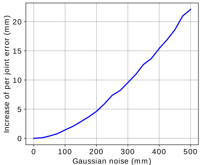
(c)

Figure 6: Ablation study of our method. In (a), we shown the error performed by each intermediate supervision. The trade off between precision (related to the number of pyramids) and speed is shown in (b), for all the pyramid levels. In (c) we present the increase in reconstruction error with respect to a Gaussian noise injected on absolute root joint position.

In Fig. 6(a), we consider each intermediate supervision of the network as a valid output and we show the improvement on accuracy (error decreasing) with respect to the number of pyramids in the network. Additionally, the error with respect to each pyramid scale is also shown. We can clearly see that all the scales are improved by the sequence of pyramids, in such a way that in the last pyramid all scales present very similar error. This evolution can be better seen in Table 5, where the error of all intermediate predictions are shown. Note that the precision of our regression method is invariant to the scale of the feature maps, since we reached excellent results with heatmaps of $4\times 4$ pixels. The same is not true for detection based approach, like in [20], since in their method the predictions are quantized by the argmax function. The error introduced by this quantization can be observed in Table 4, where we compare our regression approach with ground truth volumetric heatmaps and argmax.

Table 4: Results on Human3.6M (millimeters error), comparing predictions using ground truth heatmaps and argmax vs. our regression approach.

Method / resolution	$s=4$	$s=8$	$s=16$	$s=32$
Volumetric GT heatmaps ($s\times s\times s$) + argmax	233.9	128.6	59.9	31.0
Our regression approach (soft-argmax)	53.0	51.8	51.4	51.6

One important characteristic of our network is that it offers an excellent trade off between performance and speed. In Fig. 6(b) we show the per joint error for four pyramids with their respective scales compared to the inference speed. Note that we are able to reach 55.5 millimeters error, which is still a good result on Human3.6M, at a very fast inference rate of 200 FPS. Additionally, in Fig 7 we show the our approach is able to learn very low resolution heatmap representations, while still achieving competitive results.

Finally, we demonstrate on Fig. 6(c) the influence of a bad prediction of the absolute root depth by adding a Gaussian noise on the ground truth reference. By adding a noise of 100 millimeters (about the same magnitude of the precision of our method on MPI-INF-3DHP), we have an increase in error inferior to 2 millimeters. This clearly reinforces our idea that the error on relative joint positions is much more relevant than the absolute offset of the root joint.

Table 5: Mean per joint position error (MPJPE) in millimeters for all intermediate supervisions of the SSP-Net on Human3.6M. Odd pyramid numbers correspond to Downscaling Pyramids, and even numbers correspond to Upscaling Pyramids.

Scale	Features res.	Pyramid number / MPJPE
		1	2	3	4	5	6	7	8
$L^{0}$	$32\times 32$	-	64.1	-	55.3	-	52.4	-	51.6
$L^{1}$	$16\times 16$	85.5	65.5	60.1	55.5	55.3	52.1	51.8	51.4
$L^{2}$	$8\times 8$	71.7	67.1	58.5	57.1	53.1	53.0	52.1	51.8
$L^{3}$	$4\times 4$	68.7	-	58.9	-	54.2	-	53.0	-

(a)

(b)

(c)

(d)

(e)

Figure 7: Input image samples (a), and their respective heatmaps indirectly learned for selected joints at different pyramid levels (b, c, d, e).

5 Conclusion

In this work, we have presented a new regression method and a new scalable network architecture for 3D human pose estimation from still RGB images. The method is based on the proposed Scalable Sequential Pyramid Networks, which is a highly scalable network that can be very precise at a small computational cost and extremely fast with a small decrease in accuracy, with a single training procedure. The proposed parameter free regression approach is invariant to the resolution of feature maps thanks to the soft-argmax operation, while performing state-of-the-art scores on important benchmarks for 3D pose estimation. Additionally, we provided some intuitions about the behaviour of our method in our ablation study, which demonstrates its effectiveness, specially for efficient predictions.

6 Acknowledgements

This work was partially founded by CNPq (Brazil) - Grant 233342/2014-1.

References

- [1] D. C. Luvizon, D. Picard, H. Tabia, 2d/3d pose estimation and action recognition using multitask deep learning, in: The IEEE Conference on Computer Vision and Pattern Recognition (CVPR), 2018.
- [2] L. Pishchulin, S. Wuhrer, T. Helten, C. Theobalt, B. Schiele, Building statistical shape spaces for 3d human modeling, Pattern Recognition 67 (2017) 276 – 286. doi:https://doi.org/10.1016/j.patcog.2017.02.018.
- [3] A. Toshev, C. Szegedy, DeepPose: Human Pose Estimation via Deep Neural Networks, in: Computer Vision and Pattern Recognition (CVPR), 2014, pp. 1653–1660.
- [4] L. Pishchulin, M. Andriluka, P. V. Gehler, B. Schiele, Strong appearance and expressive spatial models for human pose estimation, in: International Conference on Computer Vision (ICCV), 2013, pp. 3487–3494.
- [5] L. Ladicky, P. H. S. Torr, A. Zisserman, Human pose estimation using a joint pixel-wise and part-wise formulation, in: Computer Vision and Pattern Recognition (CVPR), 2013.
-
[6]
D. Mehta, S. Sridhar, O. Sotnychenko, H. Rhodin, M. Shafiei, H.-P. Seidel,
W. Xu, D. Casas, C. Theobalt,
Vnect: Real-time 3d human
pose estimation with a single rgb camera, Vol. 36, 2017.
doi:10.1145/3072959.3073596.
URL http://gvv.mpi-inf.mpg.de/projects/VNect/ - [7] C.-H. Chen, D. Ramanan, 3d human pose estimation = 2d pose estimation + matching, in: The IEEE Conference on Computer Vision and Pattern Recognition (CVPR), 2017.
- [8] A. Newell, K. Yang, J. Deng, Stacked Hourglass Networks for Human Pose Estimation, European Conference on Computer Vision (ECCV) (2016) 483–499.
- [9] X. Sun, B. Xiao, F. Wei, S. Liang, Y. Wei, Integral human pose regression, in: The European Conference on Computer Vision (ECCV), 2018.
- [10] N. Sarafianos, B. Boteanu, B. Ionescu, I. A. Kakadiaris, 3d human pose estimation: A review of the literature and analysis of covariates, Computer Vision and Image Understanding 152 (2016) 1 – 20. doi:https://doi.org/10.1016/j.cviu.2016.09.002.
- [11] D. F. Atrevi, D. Vivet, F. Duculty, B. Emile, A very simple framework for 3d human poses estimation using a single 2d image: Comparison of geometric moments descriptors, Pattern Recognition 71 (2017) 389 – 401. doi:https://doi.org/10.1016/j.patcog.2017.06.024.
- [12] C. Ionescu, F. Li, C. Sminchisescu, Latent structured models for human pose estimation, in: International Conference on Computer Vision (ICCV), 2011, pp. 2220–2227.
- [13] G. Pons-Moll, D. J. Fleet, B. Rosenhahn, Posebits for monocular human pose estimation, in: 2014 IEEE Conference on Computer Vision and Pattern Recognition, 2014, pp. 2345–2352. doi:10.1109/CVPR.2014.300.
- [14] B. Tekin, I. Katircioglu, M. Salzmann, V. Lepetit, P. Fua, Structured prediction of 3d human pose with deep neural networks, in: Proceedings of the British Machine Vision Conference 2016, BMVC 2016, York, UK, September 19-22, 2016, 2016.
- [15] S. Li, W. Zhang, A. B. Chan, Maximum-margin structured learning with deep networks for 3d human pose estimation, in: The IEEE International Conference on Computer Vision (ICCV), 2015.
- [16] C. Ionescu, J. Carreira, C. Sminchisescu, Iterated second-order label sensitive pooling for 3d human pose estimation, in: 2014 IEEE Conference on Computer Vision and Pattern Recognition, 2014, pp. 1661–1668.
- [17] E. Insafutdinov, M. Andriluka, L. Pishchulin, S. Tang, E. Levinkov, B. Andres, B. Schiele, Arttrack: Articulated multi-person tracking in the wild, in: 30th IEEE Conference on Computer Vision and Pattern Recognition (CVPR 2017), IEEE, Honolulu, HI, USA, 2017, pp. 1293–1301. doi:10.1109/CVPR.2017.142.
- [18] A. Agarwal, B. Triggs, Recovering 3d human pose from monocular images, IEEE Transactions on Pattern Analysis and Machine Intelligence 28 (1) (2006) 44–58.
- [19] X. Zhou, X. Sun, W. Zhang, S. Liang, Y. Wei, Deep kinematic pose regression, Computer Vision ECCV 2016 Workshops.
- [20] G. Pavlakos, X. Zhou, K. G. Derpanis, K. Daniilidis, Coarse-to-fine volumetric prediction for single-image 3D human pose, in: Proceedings of the IEEE Conference on Computer Vision and Pattern Recognition, 2017.
-
[21]
A. Popa, M. Zanfir, C. Sminchisescu,
Deep multitask architecture for
integrated 2d and 3d human sensing, arXiv preprint arXiv:1701.08985
abs/1701.08985.
URL http://arxiv.org/abs/1701.08985 - [22] J. Martinez, R. Hossain, J. Romero, J. J. Little, A simple yet effective baseline for 3d human pose estimation, in: ICCV, 2017.
- [23] X. Sun, J. Shang, S. Liang, Y. Wei, Compositional human pose regression, arXiv preprint arXiv:1702.07432.
- [24] C. Luo, X. Chu, A. Yuille, Orinet: A fully convolutional network for 3d human pose estimation, in: BMVC, 2018.
-
[25]
D. Mehta, H. Rhodin, D. Casas, P. Fua, O. Sotnychenko, W. Xu, C. Theobalt,
Monocular 3d human pose
estimation in the wild using improved cnn supervision, in: 3D Vision (3DV),
2017 Fifth International Conference on, 2017.
URL http://gvv.mpi-inf.mpg.de/3dhp_dataset - [26] S.-E. Wei, V. Ramakrishna, T. Kanade, Y. Sheikh, Convolutional pose machines, in: IEEE Conference on Computer Vision and Pattern Recognition (CVPR), 2016.
- [27] G. Gkioxari, A. Toshev, N. Jaitly, Chained Predictions Using Convolutional Neural Networks, European Conference on Computer Vision (ECCV).
- [28] P. Hu, D. Ramanan, Bottom-up and top-down reasoning with hierarchical rectified gaussians, in: The IEEE Conference on Computer Vision and Pattern Recognition (CVPR), 2016.
- [29] A. Bulat, G. Tzimiropoulos, Human pose estimation via Convolutional Part Heatmap Regression, in: European Conference on Computer Vision (ECCV), 2016, pp. 717–732.
- [30] X. Zhou, Q. Huang, X. Sun, X. Xue, Y. Wei, Towards 3d human pose estimation in the wild: A weakly-supervised approach, in: The IEEE International Conference on Computer Vision (ICCV), 2017.
-
[31]
D. C. Luvizon, H. Tabia, D. Picard,
Human pose regression by combining
indirect part detection and contextual information, CoRR abs/1710.02322.
arXiv:1710.02322.
URL http://arxiv.org/abs/1710.02322 - [32] F. Chollet, Xception: Deep learning with depthwise separable convolutions, in: The IEEE Conference on Computer Vision and Pattern Recognition (CVPR), 2017.
- [33] A. G. Howard, M. Zhu, B. Chen, D. Kalenichenko, W. Wang, T. Weyand, M. Andreetto, H. Adam, Mobilenets: Efficient convolutional neural networks for mobile vision applications, CoRR abs/1704.04861.
- [34] C. Ionescu, D. Papava, V. Olaru, C. Sminchisescu, Human3.6m: Large scale datasets and predictive methods for 3d human sensing in natural environments, TPAMI 36 (7) (2014) 1325–1339.
- [35] M. Andriluka, L. Pishchulin, P. Gehler, B. Schiele, 2D Human Pose Estimation: New Benchmark and State of the Art Analysis, in: IEEE Conference on Computer Vision and Pattern Recognition (CVPR), 2014.
- [36] H. Zou, T. Hastie, Regularization and variable selection via the elastic net, Journal of the Royal Statistical Society, Series B 67 (2005) 301–320.