Spectroscopy and critical quantum thermometry in the ultrastrong coupling regime

Abstract

We present an exact analytical solution of the anisotropic Hopfield model, and we use it to investigate in detail the spectral and thermometric response of two ultrastrongly coupled quantum systems. Interestingly, we show that depending on the initial state of the coupled system, the vacuum Rabi splitting manifests significant asymmetries that may be considered spectral signatures of the counterintuitive decoupling effect. Using the coupled system as a thermometer for quantum thermodynamics applications, we obtain the ultimate bounds on the estimation of temperature that remain valid in the ultrastrong coupling regime. Remarkably, if the system performs a quantum phase transition, the quantum Fisher information exhibits periodic divergences, suggesting that one can have several points of arbitrarily high thermometric precision for such a critical quantum sensor.

1 Introduction

When the coupling strength between light and matter starts to be comparable with the system’s natural frequencies, the ultrastrong coupling (USC) regime of the light-matter interaction emerges [1]. The USC regime has received considerable attention from the theoretical and experimental point of view [2] during the last decade, mainly because it enables more efficient interactions that one could potentially use in quantum technologies with hybrid systems [3].

The USC regime is characterized, among other things, for the breakdown of the rotating-wave approximation (RWA) [4], an approximation commonly used in quantum optics. Unambiguous evidence of this breakdown has been acquired through spectroscopy measurements in several experiments, see for instance Refs. [5, 6, 7]. From a theoretical point of view, there are different ways to determine the spectral response of such ultrastrongly coupled quantum systems; for example, one might calculate the transmission or absorption spectra using the input-output theory [8] or through the Wiener–Khintchine power spectrum using the theory of open quantum systems [9]. A detailed treatment of the interaction between the coupled system and its environment must be done in either case. For the latter, a full microscopic derivation, sometimes called a global approach, of the corresponding master equation is the standard procedure to follow [10]. However, such derivation is highly dependent on either the coupled system is in the strong or ultrastrong coupling regime [11], and if the Born, Markov, or secular approximations have to be considered. Those approaches may then force one to opt for numerical solutions that sometimes make difficult to obtain valuable information about the problem. Here, we advocate on using the so-called time-dependent physical spectrum of light introduced by Eberly and Wódkiewicz (EW) in [12], which is based on, somehow, an operational approach. Remarkably, we find that for the case where there is a single excitation in the coupled system, which is a common situation for several up to date experiments, the EW spectrum can describe, in simple terms, some of the most interesting effects predicted to happen in the USC regime of the light-matter interaction.

On the other hand, it is known that spectroscopy measurements of a quantum system can also be used to extract information about the temperature of the thermal environment the system is in contact with. This strategy has been experimentally implemented with the name of fluorescence thermometry [13, 14]. Recently, such idea was extended to the notion of the so-called apparent temperature associated with non-thermal baths [15, 16], i.e., baths having a certain amount of quantum coherence. Along these lines of research, in this work, we use the Hopfield model [17] as an example of a composite quantum probe acting as a thermometer [18, 19], and we obtain fundamental bounds on the precision of temperature estimation. In contrast to previous works where the RWA is used [19, 20], our quantum thermometry results remain valid in the USC regime. Moreover, we exploit the thermometer’s criticality when, close to the critical point of a quantum phase transition, the corresponding quantum Fisher information, which is proportional to the square of the signal-to-noise ratio, diverges.

The organization of the paper is the following: in Sec. 2, we introduce the anisotropic Hopfield model and present a general analytical solution of the corresponding eigenfrequencies, polaritons, that we use to describe the energy level structure of the coupled system. In Sec. 3, we compute the corresponding EW spectrum and get a vacuum Rabi splitting with large asymmetries that can be considered spectral signatures of the counterintuitive decoupling effect. Sec. 4 deals with the quantum thermometry analysis, where we use the Hopfield model as a thermometer for the estimation of temperature. Sec. 5 shows the conclusions.

2 The Hopfield model

We start by writing the Hamiltonian of the simplified version of the Hopfield model  [1, 4]:

$$\hat{H}_{\rm Hopfield}=\omega_{c}\hat{a}^{\dagger}\hat{a}+\omega_{b}\hat{b}^{\dagger}\hat{b}+ig_{1}(\hat{a}\hat{b}^{\dagger}-\hat{a}^{\dagger}\hat{b})+ig_{2}(\hat{a}^{\dagger}\hat{b}^{\dagger}-\hat{a}\hat{b})+D(\hat{a}+\hat{a}^{\dagger})^{2},$$ (1)

where we have set $\hbar=1$. This kind of Hamiltonian is widely used to describe, in the weak excitation limit, several experiments dealing with the USC between two effective quantum systems [21, 6, 7, 22, 23, 24, 25, 26, 27]. For instance, in the light-matter interaction, the coupling could be between a highly confined single electromagnetic field mode of frequency $\omega_{c}$, with a collective excitation of a matter system of frequency $\omega_{b}$, which are described by the free (unperturbed) Hamiltonians $\omega_{c}\hat{a}^{\dagger}\hat{a}$ and $\omega_{b}\hat{b}^{\dagger}\hat{b}$ respectively. Often, the matter system is an ensemble made of a large number of two-level systems that can be bosonize [26]. In such case, $\hat{b}$ ($\hat{a}$) and $\hat{b}^{\dagger}$($\hat{a}^{\dagger}$) will represent, respectively, the annihilation and creation matter (field) operators with the usual commutation relation, $[\hat{b},\hat{b}^{\dagger}]=[\hat{a},\hat{a}^{\dagger}]=1$. On the third and four-term of Eq. (1), $g_{1}$ and $g_{2}$ are the coupling strengths of the commonly named corotating and counterrotating terms, respectively. Following historical convention [1, 2], we can define the USC regime of the anisotropic Hopfield model when $0.1{\omega_{c}}\leq{g}_{1,2}\leq{\omega_{c}}$ [7], where we have assumed resonant conditions $\omega_{c}=\omega_{b}$. The counterrotating terms in $\hat{H}_{\rm Hopfield}$ should not be neglected anymore if the coupled system is in the USC regime. Recall that when light interacts with natural atoms, $g_{1}$ must be equal to $g_{2}$. However, recent experiments on matter-matter interactions (specifically magnon-magnon interaction) show that one can have surprising situations where $g_{2}>g_{1}$ [7, 28]. There is also evidence that such anisotropy ($g_{1}\neq g_{2}$) can better describe the experimental data of the USC between electromagnetic radiation with artificial atoms made of superconducting quantum circuits [29]. Thus, $\hat{H}_{\rm Hopfield}$ in Eq. (1) might be called the anisotropic Hopfield model in analogy with the anisotropic Rabi model [29, 30]. The last term in Eq. (1) is the so-called diamagnetic term (because it is responsible for diamagnetism) associated with the square of the vector potential of the field and can be viewed as a self-interaction energy with $D$ its strength [1, 2]. This term is relevant and can be even dominant in the USC regime of the light-matter interaction. However, in some matter-matter interaction experiments, like the spin-magnon [31] or magnon-magnon [7], such term may not appear. Interestingly, although the anisotropic Hopfield model does not conserve the total number of excitations [1], it still preserves a discrete symmetry, the $\mathbb{Z}_{2}$ or parity symmetry [32], because $\hat{H}_{\rm Hopfield}$ commutes with the parity operator $\hat{P}=\exp\big{[}i\pi(\hat{a}^{\dagger}\hat{a}+\hat{b}^{\dagger}\hat{b})\big{]}$, i.e., the Hamiltonian is invariant under the transformation $\hat{P}^{\dagger}\hat{H}_{\rm Hopfield}\hat{P}=\hat{H}_{\rm Hopfield}$, which means that spectral crossings between energy levels from different symmetry sectors are allowed to occur [33].

It is well known that the energy level structure of $\hat{H}_{\rm Hopfield}$ is quite rich, and in the USC regime, it has substantial deviations from the standard energy spectrum obtained when the RWA is considered. This fact has been shown numerically [1] and analytically [34] for $g_{1}=g_{2}$ and $D\neq 0$. Attempts to generalize the previous results for $g_{1}\neq g_{2}$ were made very recently in [35] where, through a relatively complicated procedure, an analytical result of the eigenfrequencies was obtained. In the following, we show that, indeed, it is possible to get a complete analytical solution of the eigenvalues of $\hat{H}_{\rm Hopfield}$ in the most general case, i.e., when $g_{1}\neq g_{2}$, $D\neq 0$ and the coupled system is off-resonance $\omega_{c}\neq\omega_{b}$.

Since $\hat{H}_{\rm Hopfield}$ is a quadratic Hamiltonian, we can use a series of simple, but by no means trivial, unitary transformations to diagonalize it. We only need a combination of two rotations and one squeezing transformation that allow us to write the eigenmodes of $\hat{H}_{\rm Hopfield}$ as the Hamiltonian of two uncoupled harmonic oscillators with frequencies (see A for a detailed derivation):

$$2\,\omega_{x,y}^{2}=(2\lambda_{1}\lambda_{2}+\Omega_{x}^{2}+\Omega_{y}^{2})\pm\sqrt{\left(1-\lambda_{2}^{2}\right)(\Omega_{x}^{2}-\Omega_{y}^{2}){}^{2}+[2\lambda_{1}+\lambda_{2}(\Omega_{x}^{2}+\Omega_{y}^{2})]^{2}},$$ (2)

where $\Omega_{x}^{2}=\omega_{c}^{2}+4D\omega_{c}$, $\Omega_{y}^{2}$=$\omega_{b}^{2}$ and $\lambda_{1,2}=\left(g_{1}\pm g_{2}\right)({\omega_{c}\omega_{b}})^{\pm{1}/{2}}$. Therefore, the exact eigenvalues of $\hat{H}_{\rm Hopfield}$ are $E_{mn}=\omega_{x}(m+1/2)+\omega_{y}(n+1/2)$, with $n$ and $m$ non-negative integers. In the context of light-matter interaction, $\omega_{x,y}$ are known as the upper and lower frequencies of the photonic quasiparticles called polaritons [36], hybrid light-matter states. As expected, Eq. (2) contains, as a particular case, the results of [34, 37] and [35] when $g_{1}=g_{2}$ or $D=0$.

The analytical expressions of $\omega_{x,y}$ in Eq. (2) are useful for finding out the exact critical values of the parameters in $\hat{H}_{\rm Hopfield}$ that suppress or permit a possible quantum phase transition in the model. For instance, in order to suppress it, it is easy to show that the diamagnetic term should satisfy the inequality $D>D_{\rm crit}\equiv{(g_{1}+g_{2}){}^{2}}/({4\omega_{b}})-{\omega_{c}}/{4}$, implying that $\hat{H}_{\rm Hopfield}$ is bounded from below. For the particular case where $g_{1}=g_{2}\equiv g$, $D_{\rm crit}$ reduces to the one obtained in [38]. Additionally, if $D=0$, $\hat{H}_{\rm Hopfield}$ resembles the effective Dicke Hamiltonian in the normal phase and in the thermodynamic limit with a quantum phase transition at $g=g_{\rm crit}\equiv\sqrt{\omega_{c}\omega_{b}}/2$. However, in the superradiant phase the corresponding effective Hamiltonian of the Dicke model substantially differs from $\hat{H}_{\rm Hopfield}$, see [39] and references therein for more details.

It is instructive to see how the polaritonic frequencies $\omega_{x,y}$ and the energy eigenvalues $E_{mn}$ change when the coupled system starts to enter the USC regime. For instance, if $g_{1}=g_{2}=g$ (for simplicity), Eq. (2) reduces to

$$2\,\omega_{x,y}^{2}=(\omega_{c}^{2}+\omega_{b}^{2}+4D\omega_{c})\pm\big{[}{(\omega_{c}^{2}-\omega_{b}^{2}+4D\omega_{c}){}^{2}+16g^{2}\omega_{c}\omega_{b}}\big{]}^{\frac{1}{2}}.$$ (3)

Additionally, by considering the Thomas–Reiche–Kuhn (TRK) sum rule [40, 41, 42] in light-matter interaction, the diamagnetic term takes the value $D=g^{2}/\omega_{b}$ [34, 42]. Thus, under resonant conditions and together with the TRK sum rule, we show in Fig. 1$(a)$ the behavior of Eq. (3) as a function of the normalized coupling $g/\omega_{c}$ (solid black lines). There we can see how the frequency of the upper (lower) polariton $\omega_{x}$ ($\omega_{y}$), as its name implies, increases (decreases) as a function of $g/\omega_{c}$. If $D=0$, which can happen for some of the cases mentioned above, the behavior of Eq. (3) is shown by the red dashed lines of Fig. 1$(a)$. Contrary to the previous case, the eigenfrequency $\omega_{y}$ is now pushed to zero by increasing the normalized coupling. Then the coupled system undergoes a superradiant phase transition (SPT) (see [43, 44, 45] and references therein for a detailed discussion on the applicability of generalized no-go theorems in different light-matter scenarios like circuit-QED). It is illustrative to compare these two previous examples with the one in which the RWA has been applied, i.e., when the counterrotating and the diamagnetic terms in Eq. (2) are neglected, that is, when $g_{2}=D=0$ and $g_{1}\equiv g$. Under the RWA, the eigenfrequencies of Eq. (2) acquire a very simple form $2\omega_{x,y}^{\textsl{\tiny RWA}}\equiv({\omega_{c}+\omega_{b}})\pm\sqrt{({\omega_{c}-\omega_{b}})^{2}+4g^{2}}$ shown as the two blue dotted linear asymptotes of Fig. 1$(a)$. As expected, one can see that the RWA is a good approximation for the upper and lower polaritonic frequencies only when the normalized coupling is small enough, i.e., when the coupled system is far away from the USC regime.

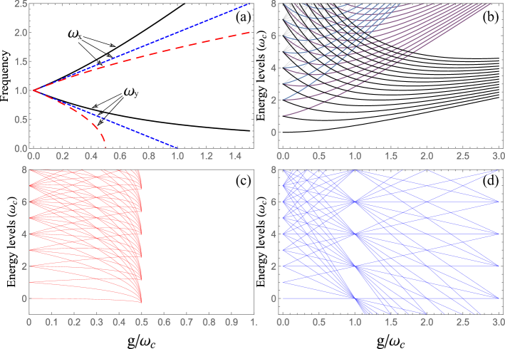
Figure 1: $\bf{(a)}$ Polaritonic frequencies $\omega_{x,y}$ of $\hat{H}_{\rm Hopfield}$, cf. Eq. (2) as a function of the normalized coupling strength $g/\omega_{c}$. Under resonance conditions ($\omega_{c}=\omega_{b}$), we set $g_{1}=g_{2}=g$ with $D=g^{2}/\omega_{b}$ (black solid lines) and $D=0$ (red dashed lines). Blue dotted lines are the frequencies obtained after the RWA is applied in Eq. (2). $\bf{(b)}$ Energy levels, $E_{mn}=\omega_{x}m+\omega_{y}n$ with $m,n\in\mathbb{Z}^{+}$, of $\hat{H}_{\rm Hopfield}$ versus $g/\omega_{c}$. The corresponding set of parameters are the same as those of the black solid lines in $\bf{(a)}$. $\bf{(c)}$ Same as $\bf{(b)}$ but now the parameters are those of the red dashed lines in $\bf{(a)}$. An evident spectral collapse occurs because $\omega_{y}$ is pushed to zero at $g_{\rm crit}=\omega_{c}/2$ where the system exhibits a super radiant phase transition [1]. $\bf{(d)}$ Same as $\bf{(b)}$ but using the parameters of the blue dotted lines of $\bf{(a)}$. As expected, all the energy-level diagrams coincide in the region $g/\omega_{c}\leq 0.1$, i.e., far away from the USC regime, see the main text for more details.

In Fig. 1$(b)$-$(d)$, we show the corresponding energy levels structure as a function of $g/\omega_{c}$, for the three cases previously discussed. For example, Fig. 1$(b)$ displays (approximately) the first $50$ energy levels $E_{mn}$ associated with the polaritonic frequencies $\omega_{x,y}$ corresponding to the solid black lines of Fig. 1$(a)$. One can see that this figure differs substantially from the figure 2.f of the recent review [1] dealing with USC between light and matter. It seems that in [1] the energy levels structure was calculated by standard numerical methods and, due to the lack of a fully converged numerical solution during the diagonalization process, fictitious avoided crossing energy levels can be observed (in Fig. 2f) for values $g/\omega_{c}\approx 1.5$. Even more, for larger values of $g/\omega_{c}$, around $3$, for example, Ref. [1] predicts an anharmonic behavior in the energy spectrum. All this is in contrast with the exact analytical result of the energy levels displayed in Fig. 1$(b)$, where due to the model’s parity symmetry, no avoided crossing energy levels are observed, and for large values of the normalized coupling strength, the energy levels are equispaced and not anharmonic as shown in [1]. In fact, in the next section, we will see in detail that such equispaced behavior is a manifestation of the so-called decoupling effect [46] occurring in the deep-strong coupling (DSC) regime. In contrast to the USC, the DSC is defined for $g/\omega_{c}>1$ [1, 2]. Figure 1$(c)$ shows the energy levels $E_{mn}$ with frequencies $\omega_{x,y}$ associated with the red dashed lines of Fig. 1$(a)$, i.e., when $D=0$ in Eq. (3). There, one can see a spectral collapse [47] at the critical coupling constant $g_{\rm crit}=\omega_{c}/2$; this happens because the corresponding $\omega_{y}$ is pushed to zero when the normalized coupling increases and the coupled system enters the SPT. Once again, in Fig. 2.f of Ref. [1] it is difficult to distinguish such spectral collapse due to an apparent deficient numerical solution. Figure 1$(d)$ also shows $E_{mn}$ but using the eigenfrequencies $\omega_{x,y}^{\textsl{\tiny RWA}}$, that correspond to the blue dotted lines of Fig. 1$(a)$, i.e., when the RWA is applied. Note that Figs. 1$(b)$-$(d)$ are shifted by adding a factor $-({\omega_{c}+\omega_{b}})/{2}$ to $E_{mn}$ and, as expected, all of them coincide in the region $g/\omega_{c}\leq 0.1$ [1, 2].

3 Spectroscopy of the Hopfield model

The Eberly-Wódkiewicz (EW) time-dependent physical spectrum is defined as [12, 48]:

$$S(\omega,t,\Gamma)=2\Gamma e^{-2\Gamma t}\int_{0}^{t}dt_{1}\int_{0}^{t}dt_{2}e^{(\Gamma-i\omega)t_{1}}e^{(\Gamma+i\omega)t_{2}}\langle\hat{a}_{1}^{\dagger}(t_{1})\hat{a}_{1}(t_{2})\rangle,$$ (4)

where $\omega$ and $\Gamma$ are the central frequency and band half-width of a Fabry–Pérot interferometer acting as a filter and $\langle\hat{a}_{1}^{\dagger}(t_{1})\hat{a}_{1}(t_{2})\rangle$ is the field’s autocorrelation function with the average done with respect to the initial state of the coupled system. If one is interested in the spectrum corresponding to the matter part of the light-matter interaction, then the previous correlation function should be replaced by $\langle\hat{b}_{1}^{\dagger}(t_{1})\hat{b}_{1}(t_{2})\rangle$. Here, we will not describe in full detail how to take into account the interaction between the ultrastrong coupled system with an environment; instead, we will see that the corresponding unitary evolution generated by the Hopfield Hamiltonian, $\hat{U}(t)=\exp(-it\hat{H}_{\rm Hopfield})$, is enough for our purposes. However, we would like to stress that the EW definition in Eq. (4) is not totally based on such unitary time-evolution. Rather, the definition is based on the microscopic fully quantum theory of light detection by Glauber and, importantly, the insertion of a frequency-sensitive device (the filter) in front of the photodetector. The use of a finite filter bandwidth, necessary on any spectrally resolved observation of a light field, makes the EW spectrum more realistic than those spectra assuming infinite spectral resolution as the Wiener–Khintchine stationary power spectrum does. In fact, due to such an operational approach in deriving the EW spectrum, this can be used to study intrinsically nonstationary light fields. For instance, in a completely lossless situation, the first theoretical prediction for the existence of the vacuum Rabi splitting was made using the EW spectrum in [49] by choosing a suitable initial state for the atom-cavity system; its impressive experimental demonstration followed this in [50]. Since then, several theoretical [51] and experimental works [52, 53] have considered the spectrometer’s finite spectral resolution in the same way that Eberly and Wódkiewicz originally proposed for theoretical comparison with their spectroscopic measurements; see also [54] for explicit time-dependent experimental spectra of resonance fluorescence.

We first consider the case where the initial state of the coupled system is $|1,0\rangle\equiv|1\rangle\otimes|0\rangle$, which means that the field initially contains one excitation (one photon) while the matter part is in its ground (vacuum) state. Additionally, and for the sake of simplicity, we assume that $g_{1}=g_{2}=g$. In such situation, we can show that the field’s autocorrelation function is given by (see B for details): $\langle 1,0|\hat{a}^{\dagger}(t_{1})\hat{a}(t_{2})|1,0\rangle=f^{*}_{1}(t_{1})f_{1}(t_{2})+2f^{*}_{2}(t_{1})f_{2}(t_{2})+f^{*}_{4}(t_{1})f_{4}(t_{2})$, with the time-dependent functions $f_{j}(t)$=$\sum_{k=1}^{2}\exp(\pm i\omega_{x}t)\mu_{jk}+\sum_{k=3}^{4}\exp(\pm i\omega_{y}t)\mu_{jk}$ and the time-independent coefficients $\mu_{jk}$ defined in (B) of  B. Notice that each $f_{j}(t)$ has a simple time-dependence given by the sum of the exponentials $\exp(\pm i\omega_{x,y}t)$, where the frequencies $\omega_{x,y}$ are those given in Eq. (3). By substituting this result in Eq. (4), one can efficiently compute the two corresponding time-integrals, where the contribution of several of the resulting time-dependent terms, in the long time limit $\Gamma t\gg 1$, are negligible due to their fast oscillations. The long time limit is when the spectrum has been stabilized and there are no significant changes. However, it should not be confused with the steady-state, which occurs when dissipation processes are explicitly taken into account; we refer the reader to Refs. [15] and [55] where this observation has been tested by analytical and numerical methods in other examples of the light-matter interaction. Therefore, in the long time limit and with the particular initial conditions above-mentioned, the EW spectrum of Eq. (4) can be very well approximated by the time-independent expression $S(\omega,\Gamma)\equiv S_{x}(\omega,\Gamma)+S_{y}(\omega,\Gamma)$, where we have defined the following terms:

$$S_{x,y}(\omega,\Gamma)=\frac{\frac{1}{2}\Gamma_{x,y}}{\Gamma^{2}+(\omega-\omega_{x,y})^{2}},\quad\Gamma_{x,y}=\frac{\Gamma h_{x,y}}{4\omega_{c}^{2}\omega_{x,y}^{2}}\big{[}(\omega_{c}+\omega_{x,y})^{4}+2(\omega_{c}^{2}-\omega_{x,y}^{2})^{2}\big{]},$$ (5)

$h_{x,y}=\big{[}{1}\pm{\Omega}(4\lambda^{2}+\Omega^{2})^{-\frac{1}{2}}\big{]}^{2}/4$, $\Omega={\omega_{c}}^{2}+4D\omega_{c}-{\omega_{b}}^{2}$ and $\lambda=2g\sqrt{\omega_{b}\omega_{c}}$. Thus, for the initial state $|1,0\rangle$, which contains only a single excitation in the coupled system, the EW spectrum of the Hopfield Hamiltonian is just the sum of two Lorentzian line shape functions $S_{x,y}(\omega,\Gamma)$. This analytical spectrum is valid in the USC regimen for any value of the diamagnetic term $D$, and it is one of our major results. It is illustrative to compare this result with the corresponding spectrum that is obtained under the RWA and the same initial state $|1,0\rangle$; in such case, the calculations are more straightforward than the previous ones and the EW spectrum reduces to $S_{\textsl{\tiny RWA}}(\omega,\Gamma)=S_{x}^{\textsl{\tiny RWA}}(\omega,\Gamma)+S_{y}^{\textsl{\tiny RWA}}(\omega,\Gamma)$, where

$$S_{x,y}^{\textsl{\tiny RWA}}(\omega,\Gamma)=\frac{\frac{1}{2}\Gamma_{\textsl{\tiny RWA}}}{\Gamma^{2}+\big{(}\omega-\omega_{x,y}^{\textsl{\tiny RWA}}\big{)}^{2}},\quad\Gamma_{\textsl{\tiny RWA}}=\frac{4\Gamma g^{2}}{(\omega_{b}-\omega_{c})^{2}+4g^{2}}\qquad\qquad\quad$$ (6)

and $2\omega_{x,y}^{\textsl{\tiny RWA}}=({\omega_{c}+\omega_{b}})\pm\sqrt{({\omega_{c}-\omega_{b}})^{2}+4g^{2}}$ are the eigenfrequencies that were already obtained in Sec. 2. The main difference between the Lorentzians of Eq. (5) and Eq. (6) is that, in the latter, the corresponding $\Gamma_{\textsl{\tiny RWA}}$ of each $S_{x,y}^{\textsl{\tiny RWA}}(\omega,\Gamma)$ is the same, while in the former each $\Gamma_{x,y}$ is different. Later, we will see that this difference is the root of the asymmetric shape of the vacuum Rabi splitting of a system that is in the USC regimen of the light-matter interaction. One thing in common between all the Lorentzian functions in the equations mentioned above is that, as a function of $\omega$, each of them is centered around the corresponding eigenfrequency, i.e., $S_{x,y}(\omega,\Gamma)$ is centered at $\omega_{x,y}$ and $S_{x,y}^{\textsl{\tiny RWA}}(\omega,\Gamma)$ at $\omega_{x,y}^{\textsl{\tiny RWA}}$. This is because the spectrum’s maximum intensity is expected to happens at the resonant frequencies that can be obtained from the transitions between two energy levels of the coupled system; for example, by defining the polariton dispersion as $\Delta E_{pq}^{mn}\equiv E_{mn}-E_{pq}=(m-p)\omega_{x}+(n-q)\omega_{y}$, which is the energy associated with such transitions, $\Delta E^{10}_{00}=\omega_{x}$ and $\Delta E^{01}_{00}=\omega_{y}$ represent the transitions from the first two excited states to the ground state of the Hopfield Hamiltonian.

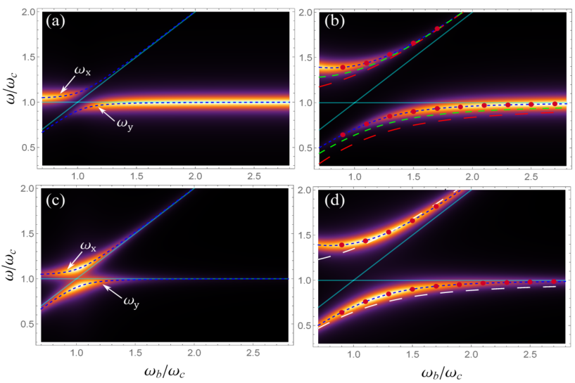
Figure 2: Field spectra of the Hopfield model in the USC regime and within the single excitation manifold. For $\bf{(a)}$-$\bf{(b)}$ the initial state of the light-matter coupled system is $|1,0\rangle$, i.e., the excitation starts in the field while the matter is in its ground state; for $\bf{(c)}$-$\bf{(d)}$ we have the opposite initial state, $|0,1\rangle$. Density plots of $\bf{(a)}$,$\bf{(c)}$ are for $g=0.1\omega_{c}$ and $\bf{(b)}$,$\bf{(d)}$ for $g=0.35\omega_{c}$, in all cases the diamagnetic constant is $D=g^{2}/\omega_{b}$ and $\Gamma=0.05\omega_{c}$. When the normalized coupling constant $g/\omega_{c}$ increases, the separation of the avoiding crossing between the polariton branches also increases. Brighter (darker) colors are the regions where the intensity of the spectrum is high (low). Cyan solid lines are the bare frequencies $\omega_{c}$ and $\omega_{b}$ of the uncoupled ($g=0$) system. All dashed lines are the polaritonic dispersions representing the energy transition between the first two excited states of $\hat{H}_{\rm Hopfield}$ with the ground state. For the blue dashed lines, we set $D=g^{2}/\omega_{b}$ and the polariton dispersions coincide with the values where the spectrum’s intensity is maximum, depicted as the red dots in $\bf{(b)}$,$\bf{(d)}$. For the red dashed lines, we set $D=0$, corresponding to the case of Fig.1$\bf{(c)}$. The green dashed lines of $\bf{(b)}$ are for $D=0.5g^{2}/\omega_{b}$, while in $\bf{(d)}$ the white dashed lines are for $D=g_{2}=0$ and $g_{1}=g$, i.e., it is the situation where only the corotating terms are present in the Hopfield Hamiltonian. See the main text for more details.

In Fig. 2$(a)$-$(b)$, we show density-plots of the spectrum of the Hopfield model, $S(\omega,\Gamma)=S_{x}(\omega,\Gamma)+S_{y}(\omega,\Gamma)$, as a function of $\omega_{b}/\omega_{c}$ with a normalized coupling strength $g/\omega_{c}$ equal to $0.1$ (a) and $0.35$ (b), i.e., the system is within the USC regime. Brighter (darker) colors represent the regions where the intensity of the spectrum is high (low). Near resonance ($\omega_{b}/\omega_{c}=1$), one can see the characteristic avoiding crossing between the upper and lower polaritons branches of the coupled system. As expected, when the normalized coupling $g/\omega_{c}$ increases, the separation between these two branches also increases. In Fig. 2$(a)$-$(b)$ we also show, as dashed-lines, the corresponding polariton dispersions $\Delta E_{00}^{10}$ and $\Delta E_{00}^{01}$ as a function of $\omega_{b}/\omega_{c}$ and for different values of the diamagnetic constant $D$. For example, by considering the TRK sum rule [41, 42], we have that $D=g^{2}/\omega_{b}$ [40, 1] (blue dashed-lines). The blue-dashed lines fit very well within the regions where the spectrum’s intensity is maximum, see the red dots. The green dashed lines are for $D=dg^{2}/\omega_{b}$, where $d\in(0,1)$ is a prefactor that effectively reduces the diamagnetic term’s strength. Such a value of $D$ represents a modification of the standard Hopfield model under the TRK sum rule; it was introduced very recently in [23] to explain the experimental data of Landau polaritons in highly nonparabolic two-dimensional gases in the USC regime; for Fig. 2$(b)$ we set $d=0.5$. The red dashed lines are for $D=0$ and represent the case described in Fig. 1$(c)$, i.e., a situation where the corotating and counterrotating terms are taken into account, but the diamagnetic term is not present. The cyan solid lines represent the bare frequencies $\omega_{c}$ and $\omega_{b}$ of the system; in particular, the horizontal cyan line corresponds to the field frequency $\omega_{c}$. It is easy to show that in the dispersive regime ($\omega_{b}/\omega_{c}\gg 1$), $\omega_{x,y}\approx\omega_{b,c}$; that is why for an initial state like $|1,0\rangle$ the spectrum of the field is brighter near the horizontal cyan line representing $\omega_{c}$. In the dispersive regime there is little exchange of energy between the field and the matter part. Therefore, any initial excitation in the field will remain mainly there and should be captured by the EW spectrum around $\omega_{c}$.

As a complementary case, we now consider that in the Hopfield model the field starts in the vacuum and the matter part in its first excited state, i.e., the entire initial state is $|0,1\rangle\equiv|0\rangle\otimes|1\rangle$, opposite situation of the previous example. In this case, the field’s autocorrelation function will be (see B): $\langle 0,1|\hat{a}^{\dagger}(t_{1})\hat{a}(t_{2})|0,1\rangle=f^{*}_{2}(t_{1})f_{2}(t_{2})+f^{*}_{3}(t_{1})f_{3}(t_{2})+2f^{*}_{4}(t_{1})f_{4}(t_{2})$, where, as in the previous example, we have assumed $g_{1}=g_{2}=g$. In the long-time limit, the corresponding EW spectrum can be written as $S^{\prime}(\omega,\Gamma)\equiv{S}^{\prime}_{x}(\omega,\Gamma)+{S}^{\prime}_{y}(\omega,\Gamma)$, where

$${S}^{\prime}_{x,y}(\omega,\Gamma) =\frac{\Gamma^{\prime}_{x,y}}{\Gamma^{2}+(\omega-\omega_{x,y})^{2}},\,\,\,\,\Gamma^{\prime}_{x,y}=\frac{\Gamma h_{xy}}{32\omega_{b}\omega_{c}\omega_{x,y}^{2}}(3\omega_{b}^{2}-2\omega_{b}\omega_{x,y}+3\omega_{x,y}^{2})(\omega_{c}+\omega_{x,y})^{2},$$ (7)

$h_{xy}=(4\lambda^{2})(4\lambda^{2}+\Omega^{2})^{-1}$, $\Omega={\omega_{c}}^{2}+4D\omega_{c}-{\omega_{b}}^{2}$ and $\lambda=2g\sqrt{\omega_{b}\omega_{c}}$. Once again, we obtain that for the single excitation regime, but with the initial state $|0,1\rangle$, the Hopfield model’s spectrum can be well approximated by the sum of two Lorentzian $S^{\prime}_{x,y}(\omega,\Gamma)$ having different $\Gamma^{\prime}_{x,y}$.

For the initial state $|0,1\rangle$, Figs. 2$(c)$-$(d)$ show density-plots of the spectrum of the field $S^{\prime}(\omega,\Gamma)=S_{x}^{\prime}(\omega,\Gamma)+S_{y}^{\prime}(\omega,\Gamma)$. We set the normalized coupling $g/\omega_{c}$ as $0.1$ (c) and $0.35$ (d). Like in the previous case, dashed-lines are the polaritonic dispersion from the first two excited states to the ground state. In particular, blue dashed-lines are for $D=g^{2}/\omega_{b}$ while white dashed-lines are for $D=g_{2}=0$ and $g_{1}=g$, i.e., the white dashed-lines represent the situation described in Fig. 1$(d)$ where only corotating terms in the Hamiltonian are considered. As expected, the blue dashed lines match the values where the intensity of the spectrum is maximum and illustrated by the red dots in $(d)$. Notice that, contrary to Fig. 2$(a)$-$(b)$, the intensity of the spectrum is now higher around the avoiding crossing region (near resonance). Moreover, in the dispersive limit, the spectrum’s intensity vanishes nearby both solid cyan lines. Such behavior occurs because the initial state is $|0,1\rangle$ and, therefore, there will not be enough energy to be captured by the spectrum of the field when $\omega_{b}/\omega_{c}\gg 1$. In contrast, near resonance, there is a strong exchange of energy between light and matter; thus, high values in the intensity of the field’s spectrum can be obtained.

3.1 Asymmetries in the vacuum Rabi splitting

From previous results, we can quickly obtain the vacuum Rabi splitting (VRS) of the light-matter interaction in the Hopfield model when the bare frequencies of the field and matter, $\omega_{c}$ and $\omega_{b}$, are resonant, $\omega_{c}=\omega_{b}$. In particular, in Fig. 3$(a)$ we show a density plot for the EW spectrum of the field $S(\omega,\Gamma)=S_{x}(\omega,\Gamma)+S_{y}(\omega,\Gamma)$, as a function of the normalized coupling $g/\omega_{c}$ and frequency $\omega/\omega_{c}$, at resonance conditions $\omega_{c}=\omega_{b}$ and with the diamagnetic constant under the TRK sum rule $D=g^{2}/\omega_{b}$. Red (blue) colors are the regions where the spectrum’s intensity is high (low). For $g>0.1\omega_{c}$, we see that the spectrum is not symmetric with respect to the resonance frequency and heights because of $\Gamma_{x}\neq\Gamma_{y}$. This asymmetry and the separation between the peaks of the two Lorentzian, $S_{x}(\omega,\Gamma)$ and $S_{x}(\omega,\Gamma)$, increases for larger values of $g/\omega_{c}$ and it is more evident in Fig. 3$(b)$; there we show, in semi-log scale, the VRS for three different values of the normalized coupling constant indicated by the dark arrows of Fig. 3$(a)$. In Fig. 3$(b)$ the right Lorentzian $S_{x}(\omega,\Gamma)$ becomes dominant while the left one $S_{y}(\omega,\Gamma)$ decreases as the coupling constant increases; the blue dashed line is for $g=0.1\omega_{c}$, green dashed-line is for $g=0.35\omega_{c}$, and the solid black line is for $g/\omega_{c}=1$. The first two cases are in the USC regime, and the last one starts to enter the DSC regime. For the sake of comparison, the red solid-line of Fig. 3$(b)$ shows the VRS, but when the RWA has been applied, i.e., it represents $S_{\textsl{\tiny RWA}}(\omega,\Gamma)=S_{x}^{\textsl{\tiny RWA}}(\omega,\Gamma)+S_{y}^{\textsl{\tiny RWA}}(\omega,\Gamma)$ for $g=0.35\omega_{c}$; thus, under the RWA, the VRS will be symmetric to the heights and the resonance frequency. We might understand the asymmetric behavior of the VRS by looking for the eigenfrequencies $\omega_{x,y}$ in the limit where the normalized coupling is large. For instance, using Eq. (3) it is easy to show that if $D=g^{2}/\omega_{b}$ and $g\gg 1$, then $\omega_{x}^{2}\approx 4g^{2}\omega_{c}/\omega_{b}$, $\omega_{y}^{2}\approx 0$ and the eigenvalues $E_{mn}$ of $\hat{H}_{\rm Hopfield}$ simplify to those of a single harmonic oscillator $E_{mn}\approx\tilde{\omega}_{x}(m+1/2)$, with $\tilde{\omega}_{x}\equiv 2g\sqrt{\omega_{c}/\omega_{b}}$. In such limit, the EW spectrum of the field reduces to just one Lorentzian give by $S(\omega,\Gamma)\approx\tilde{S}_{x}(\omega,\Gamma)$, where

$$\tilde{S}_{x}(\omega,\Gamma)\equiv\frac{3\Gamma g^{2}/(2\omega_{b}\omega_{c})}{\Gamma^{2}+(\omega-\tilde{\omega}_{x})^{2}}.$$ (8)

Thus, we see that in the DSC regime of the Hopfield model one of the two characteristic peaks of the VRS tends to vanish and the other remains and get more prominent, actually, in Refs. [27, 56, 57] significant asymmetries of the VRS were experimentally obtained, confirming the breakdown of the RWA and the relevance of the diamagnetic term in the USC and DSC regime. Having in mind that a measurement of the separation between these two peaks gives the information about how strong the light-matter coupling is, one can interpret the above tendency into a single peak as an effective decoupling between light and matter when the coupling constant increases, a counterintuitive effect predicted in Ref. [46] and measured in Ref. [21] by reaching the astonishing record $g/\omega_{c}=1.8$ at room temperature. The effective decoupling happens because the diamagnetic term, which is proportional to $g^{2}$ under the TRK sum rule, is the dominant term in the DSC regime, and it can act as a potential barrier [1] for the photonic field producing the collapse of the Purcell effect [46].

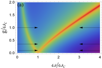
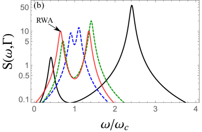
Figure 3: Vacuum Rabi splitting (VRS) of the Hopfield model. $\bf{(a)}$ Shows the spectrum of the field $S(\omega,\Gamma)=S_{x}(\omega,\Gamma)+S_{y}(\omega,\Gamma)$, cf. Eq.(5), as a function of the normalized coupling strength $g/\omega_{c}$ and frequency $\omega/\omega_{c}$, at resonance conditions, $\omega_{c}=\omega_{b}$. Red (blue) colors are the regions where the intensity of the spectrum is high (low). In the USC regime the VRS is no longer symmetric with respect to the resonance frequency and the heights of each polariton branch. In fact, for large coupling strengths, the diamagnetic term in $\hat{H}_{\rm Hopfield}$ is dominant, and the VRS tends to a single polariton branch, which can be interpreted as an effective decoupling effect [46]. $\bf{(b)}$ Shows, in a semi-log scale, the VRS for three different values of $g/\omega_{c}$ indicated by the dark arrows of $\bf{(a)}$. Blue dashed line is for $g=0.1\omega_{c}$, green dashed line for $g=0.35\omega_{c}$ and black solid line for $g=\omega_{c}$. In particular, the red solid line is for $g=0.35\omega_{c}$, but when the rotating-wave approximation (RWA) has been applied to $\hat{H}_{\rm Hopfield}$. Under this approximation the VRS is fully symmetric. In all cases the diamagnetic constant is $D=g^{2}/\omega_{b}$ and $\Gamma=0.05\omega_{c}$.

It is essential to mention that the asymmetry of the VRS remains, but it is less noticeable (plots not shown) if one uses $|0,1\rangle$ as the initial state in the calculations of the EW spectrum, i.e., the field starts in the vacuum state while matter contains one excitation; the corresponding spectrum is $S^{\prime}(\omega,\Gamma)=S^{\prime}_{x}(\omega,\Gamma)+S^{\prime}_{y}(\omega,\Gamma)$. This observation might explain why in a recent experimental demonstration of the vacuum Bloch-Siegert shift, the VRS looks almost symmetric even when $g/\omega_{c}=0.36$ [6]. In fact, in [6], the USC is between a two-dimensional electron gas with the counter-rotating component of a terahertz photonic-crystal cavity’s vacuum fluctuation field, realizing a strong-field phenomenon without a strong field [26]. Finally, we notice that similar spectral modifications have been pointed out in other theoretical works [8, 58, 11, 59]; however, they use more involved dissipative models to obtain these results. Here, we remark that our analytical expressions allow us to characterize in simple terms the spectral response of these two ultrastrongly coupled quantum systems.

4 Quantum thermometry with the Hopfield model

Similar to standard quantum thermometry studies using individual quantum probes as thermometers [18, 60, 61], we assume that our thermometer (made of the two interacting quantum systems described by $\hat{H}_{\rm Hopfield}$) is fully thermalized by allowing it to equilibrate with the sample to be probed. The temperature $T$ of the sample is inferred from the thermal state of the probe $\hat{\rho}_{T}\equiv\exp(-\beta\hat{H}_{\rm Hopfield})/Z$, where $Z$ is the partition function, $\beta=(k_{B}T)^{-1}$ is the inverse temperature and $k_{B}$ is the Boltzmann constant. To determine the ultimate limit on the estimation of temperature, we need to resort to the quantum Cramér-Rao bound [19] given by $\Delta T\geq 1/\sqrt{N\mathcal{F}(\hat{\rho}_{T})}$, where $\Delta T$ is the uncertainty in the temperature, $N$ the number of independent measurements and $\mathcal{F}(\hat{\rho}_{T})$ is the quantum Fisher information (QFI). For thermal states, the QFI can be written in terms of the variance of the thermometer’s Hamiltonian $\mathcal{F}(\hat{\rho}_{T})=(\Delta\hat{H}_{\rm Hopfield})^{2}/(k_{B}^{2}T^{4})$, where $(\Delta\hat{H}_{\rm Hopfield})^{2}\equiv\langle\hat{H}^{2}_{\rm Hopfield}\rangle-\langle\hat{H}_{\rm Hopfield}\rangle^{2}$. We can rewrite the QFI in terms of the thermometer’s heat capacity as $\mathcal{F}(\hat{\rho}_{T})=C(T)/(k_{B}T^{2})$, where $C(T)=(\Delta\hat{H}_{\rm Hopfield})^{2}/(k_{B}T^{2})$, which implies that for the single-shot scenario of $N=1$ [60], the signal-to-noise ratio, $T/\Delta T$, is upper bounded as $(T/\Delta T)^{2}\leq C(T)/k_{B}$. Moreover, the heat capacity can also be obtained from the internal energy, $U$, as follow: $C(T)=\partial_{T}U$, with $U=k_{B}T^{2}\partial_{T}\ln Z$ [62]. Thus, we only need to know how the thermometer’s partition function is to obtain the corresponding ultimate bound on the thermal sensitivity through the QFI. To compute $Z={\rm tr}\{\exp(-\beta\hat{H}_{\rm Hopfield})\}$, we will take advantage of the analytical solution of the Hopfield model given in Sec. 2. For instance, the trace operation is independent of the representation, so we can calculate $Z$ in the normal mode representation where $\hat{H}_{\rm Hopfield}$ is diagonal, and it represents two decoupled oscillators with eigenfrequencies $\omega_{x,y}$, Eq. (2). On such basis, the partition function of two independent quantum system factorizes as $Z=Z_{x}Z_{y}$, where $Z_{x,y}=\frac{1}{2}{\rm csch}(\beta\omega_{x,y}/2)$ is the partition function of a quantum harmonic oscillator in a thermal state [62]. We can efficiently compute the internal energy and the heat capacity as $U=U_{x}+U_{y}$ and $C(T)=C_{x}(T)+C_{y}(T)$, where $U_{x,y}=\frac{1}{2}\omega_{x,y}\coth(\beta\omega_{x,y}/2)$ and $C_{x,y}(T)=\frac{1}{4}k_{B}(\beta\omega_{x,y})^{2}{\rm csch}^{2}(\beta\omega_{x,y}/2)$. Therefore, the QFI of the anisotropic Hopfield model acting as a thermometer reduces to $\mathcal{F}(\hat{\rho}_{T})=\mathcal{F}_{x}(\hat{\rho}_{T})+\mathcal{F}_{y}(\hat{\rho}_{T})$, where

$$\mathcal{F}_{x,y}(\hat{\rho}_{T})=\Big{(}\frac{\omega_{x,y}}{2k_{B}T^{2}}\Big{)}^{2}{\rm csch}^{2}\bigg{(}\frac{\omega_{x,y}}{2k_{B}T}\bigg{)}$$ (9)

is the well known QFI of a harmonic oscillator [60, 15].

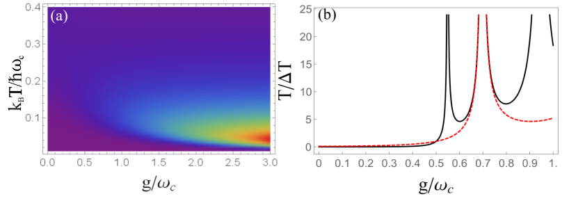
Figure 4: $\bf{(a)}$ Quantum Fisher information (QFI) of the composite quantum probe, $\mathcal{F}(\hat{\rho}_{T})=\mathcal{F}_{x}(\hat{\rho}_{T})+\mathcal{F}_{x}(\hat{\rho}_{T})$, cf. Eq. (9), as a function of the normalized coupling $g/\omega_{c}$ and the scaled temperature $k_{B}T/\hbar\omega_{c}$. Red (blue) colors represent high (low) values of $\mathcal{F}(\hat{\rho}_{T})$. The QFI substantially increases if the probe is in the USC regime. The set of parameters are those used in Fig. 1(b), i.e., the system is on resonance $\omega_{c}=\omega_{b}$, $g_{1}=g_{2}=g$ and $D=g^{2}/\omega_{b}$. $\bf{(b)}$. Signal-to-noise ratio, $T/\Delta T\equiv T\sqrt{\mathcal{F}(\hat{\rho}_{T})}$, versus $g/\omega_{c}$, with a scaled temperature $k_{B}T/\hbar\omega_{c}=0.05$ (black solid line) and $k_{B}T/\hbar\omega_{c}=0.1$ (red dashed line). For this case $D=0$ and $\mathcal{F}(\hat{\rho}_{T})$ is given by Eq. (10). At low temperatures a divergence of $T/\Delta T$ appears if the system is close to the critical point ($g_{\rm crit}\equiv\omega_{c}/2$) of the quantum phase transition described in Fig. 1(c). If $g>g_{\rm crit}$, periodic divergences occur because one of hyperbolic functions of Eq. (10) changes to its trigonometric version. In principle, one could obtain arbitrarily high thermometry precision by exploiting the criticality of this quantum sensor.

In Fig. 4$(a)$, we show $\mathcal{F}_{x}(\hat{\rho}_{T})+\mathcal{F}_{y}(\hat{\rho}_{T})$ as a function of the temperature and the normalized coupling using the same set of parameters of Fig. 1$(b)$, i.e., a situation where the interacting systems are on resonance $(\omega_{c}=\omega_{b})$, the diamagnetic constant is obtained from the TRK sum rule ($D=g^{2}/\omega_{b}$), and the contribution of the co-rotating and counter-rotating terms is the same $(g_{1}=g_{2}=g)$; red (blue) colors represent high (low) values of the QFI. We can see that for any value of the temperature the QFI substantially increases, and the thermometry precision as well, when the thermometer operates in the USC and DSC regime. Similar results were obtained in Refs. [20, 19] but for the particular case in which the RWA is used in the Hamiltonian of two coupled bosonic modes. If we replace $\omega_{x,y}$ by $\omega_{x,y}^{\textsl{\tiny RWA}}$ in Eq. (9), we obtain the same expression of the QFI derived in [20, 19].

Such enhancement in the estimation of the temperature is due to the fact that the gap between the corresponding energy levels of the thermometer decreases when the coupling constant increases, see Fig. 1$(b)$, which makes it easy to populate more excited energy states. Therefore, in an extreme case where the gap vanishes, significant thermometry precision changes are to be expected [19]. Interestingly, a vanishing gap occurs during the spectral collapse of Fig. 1$(c)$, where $D=0$ and $\hat{H}_{\rm Hopfield}$ represents a Dicke-type Hamiltonian with a quantum phase transition at the critical point $g_{\rm crit}\equiv{\omega_{c}}/2$, see Sec. 2. In such a case, the eigenfrequencies of Eq. (3) simplify to $\omega^{2}_{x,y}=\omega_{c}^{2}\pm 2g\omega_{c}$, which we substitute in Eq. (9) to get

$$\mathcal{F}(\hat{\rho}_{T})=\frac{\omega_{c}^{2}+2g\omega_{c}}{4k_{B}^{2}T^{4}}{\rm csch}^{2}\bigg{(}\frac{\sqrt{\omega_{c}^{2}+2g\omega_{c}}}{2k_{B}T}\bigg{)}+\frac{\omega_{c}^{2}-2g\omega_{c}}{4k_{B}^{2}T^{4}}{\rm csch}^{2}\bigg{(}\frac{\sqrt{\omega_{c}^{2}-2g\omega_{c}}}{2k_{B}T}\bigg{)}.$$ (10)

When $g=g_{\rm crit}$ the first term in the above equation vanishes at low temperatures, while the second one is proportional to $T^{-2}$, making the QFI diverge. This divergence suggests that an arbitrarily high thermometry precision can be achieved in the critical region’s vicinity at low enough temperatures [19]. However, since $C(T)=\mathcal{F}(\hat{\rho}_{T})k_{B}T^{2}$, the $T^{-2}$ dependency of the QFI implies that $C(T)$ will remain constant even at $T=0$; this is, somehow, a contradiction with the Third Law of thermodynamics, where it is generally assumed that for any system with a finite energy gap, the heat capacity should vanish (exponentially) at $T=0$. In fact, this vanishing of the heat capacity is why it is so difficult to estimate low temperatures. To be more specific, the relative error $(\Delta T/T)^{2}\geq k_{B}/C(T)$ necessary diverges exponentially as $T\rightarrow 0$ [63]. Nevertheless, finite quantum dissipation may restore the Third Law [64], indicating that important effects resulting from the coupling to the environment may not be neglected. Remarkably, if $g>g_{\rm crit}$ several divergences in the QFI may appear, which is our second major result; such atypical behavior of the QFI when $g>g_{\rm crit}$ is due to the argument on the hyperbolic function in the second term of Eq. (10) which becomes complex (purely imaginary), this changes the hyperbolic cosecant to its trigonometric version, which as a function of the normalized coupling has periodic divergences that can be tailored depending on the temperature. Recall that in the region $g>g_{\rm crit}$ the energy level structure of the coupled system is no longer discrete but continuous. Using Eq. (10), we plot in Fig. 4$(b)$ the signal-to-noise ratio ${T}/{\Delta T}\equiv T\sqrt{\mathcal{F}(\hat{\rho}_{T})}$ as a function of the normalized coupling; the solid black line shows the above-mentioned periodic divergences of the QFI at low temperatures, and these are modified if the temperature increases, see the red dashed line. We would like to point out that, at first glance, one would expect $T/\Delta T$ to diverge at the quantum critical point; however, this is not what we see in Fig. 4$(b)$. Actually, it is easy to show that each divergence in Fig. 4$(b)$ is located at ${g}/\omega_{c}=\frac{1}{2}+2(k_{B}Tn\pi)^{2}$, with $n\in\mathbb{N}$. The physical reason is that at equilibrium, which is the case we are considering, the critical point is shifted by the temperature. Another well-known example where this fact occurs is the Dicke model, in which, by following a mean-force approach and an optimization procedure in the free energy of each two-level atom, one can obtain the critical coupling $\lambda_{c}$ of its equilibrium transition (see Eq. (9) of [65]): $\lambda_{c}=\frac{1}{2}\sqrt{\omega_{c}\omega_{z}\coth\left({\beta\omega_{z}}/{2}\right)}$, where $\omega_{c}$ and $\omega_{z}$ are the frequencies of the cavity field and the two-level atomic transition respectively and $\beta$ is the inverse temperature. This critical coupling reduces to $\lambda_{c}=\sqrt{\omega_{c}\omega_{z}}/2$ when $\beta\rightarrow\infty$, the expected result of the corresponding quantum phase transition. Similar results, at zero temperature, were recently obtained in [66] but only for frequency-estimation protocols, where the criticallity of finite-component quantum optical probes was exploited.

5 Conclusions

We have shown that the spectral response of two ultrastrongly coupled quantum systems (described by the Hopfield model) can be characterized by the Eberly-Wódkiewicz (EW) physical spectrum. Through a non-trivial diagonalization procedure, we derived an exact analytical solution of the anisotropic Hopfield Hamiltonian, and we found the corresponding polaritonic frequencies, see Eq. (2), as well as the autocorrelation function of the field. The eigenfrequencies were useful to obtain a better description (compared with previous numerical results [1]) of the energy level structure of the coupled system, including its quantum phase transition. Simultaneously, the autocorrelation function was necessary to perform the two time-integrals of the EW spectrum. In the long-time limit, the resulting EW spectrum is time-independent and it can be reduced to a simple expression, Eq. (5), that remains valid in the USC and DSC regime. We confirm that in the DSC regime, the vacuum Rabi splitting manifests large asymmetries that can be considered spectral signatures of the counterintuitive decoupling effect.

We also show that when the Hopfield model is used as a quantum thermometer, the corresponding ultimate bounds on the estimation of temperature are valid in the USC and DSC regime; regimes that, to the best of our knowledge, had not been explored yet in the field of quantum thermometry. For both regimes, the quantum Fisher information (QFI) of the Hopfield model substantially increases. Remarkably, when the coupled system (described by a Dicke-type Hamiltonian) performs a superradiant phase transition (SPT), the QFI displays periodic divergences that allow it to have, in principle, arbitrary high thermometry precision. This thermometry result depends on the fact that the diamagnetic term should not be present in the USC and DSC regime; therefore, it might not be possible to test it in quantum optics experiments where light interacts with natural atoms. However, it could be implemented in condensed matter systems using matter-matter interactions; for instance, Dicke cooperativity was experimentally realized in [31] with spin-magnon interactions in the USC regime. Moreover, recent terahertz magnetospectroscopy experiments [7, 28, 67] suggest that the magnonic version of the SPT is within reach [68].

Using the Hopfield model’s analytical solution presented in this work, it would be possible to derive the corresponding microscopic (global) Lindblad master equation [10]. With the master equation at hand, one could investigate the impact of the USC on the energy transfer dynamics or the thermodynamics properties [69]. Moreover, it is known that the output power of a particular class [70] of quantum heat engines is determined by the heat capacity of their working substance [71]; therefore, if we use the Hopfield model as a working medium, significant changes in its heat capacity are expected to enhance the maximal output power of such a critical heat engine operating in the USC regime [72]. These are a few exciting topics of research that we will address in future work.

Note added. After completing this manuscript, we became aware of related work [35], which considers a general solution of two interacting harmonic oscillators resembling the anisotropic Hopfield model.

Appendix A Diagonalization of the anisotropic Hopfield Hamiltonian

In this Appendix, we describe all the necessary steps to diagonalize the anisotropic ($g_{1}\neq g_{2}$) Hopfield Hamiltonian $\hat{H}_{\rm Hopfield}$ given in Eq. (1) of the main text. First, we make a change of sign on the third and four term of $\hat{H}_{\rm Hopfield}$ by means of the unitary transformation $\hat{T}=\exp(-i{\pi}\hat{b}^{\dagger}\hat{b}/2)$, i.e., $\hat{T}\hat{H}_{\rm Hopfield}\hat{T}^{\dagger}\equiv\hat{H}_{1}$, where $\hat{T}\hat{b}\hat{T}^{\dagger}=i\hat{b}$, $\hat{T}\hat{b}^{\dagger}\hat{T}^{\dagger}=-i\hat{b}^{\dagger}$ such that

$$\hat{H}_{1}=\omega_{c}\hat{a}^{\dagger}\hat{a}+\omega_{b}\hat{b}^{\dagger}\hat{b}+g_{1}(\hat{a}\hat{b}^{\dagger}+\hat{a}^{\dagger}\hat{b})+g_{2}(\hat{a}^{\dagger}\hat{b}^{\dagger}+\hat{a}\hat{b})+D(\hat{a}+\hat{a}^{\dagger})^{2}.$$ (11)

Next, we rewrite $\hat{H}_{1}$ in terms of the hermitian operators $\hat{x}$, $\hat{p}_{x}$, $\hat{y}$ and $\hat{p}_{y}$, defined by the relations $\hat{a}=\sqrt{{\omega_{c}}/{2}}\big{(}\hat{x}+{i}\hat{p}_{x}/\omega_{c}\big{)}$, $\hat{b}=\sqrt{{\omega_{b}}/{2}}\big{(}\hat{y}+{i}\hat{p}_{y}/{\omega_{b}}\big{)}$ and their adjoint operators, evidently $[\hat{x},\hat{p}_{x}]=i$ and $[\hat{y},\hat{p}_{y}]=i$. This yields

$$\hat{H}_{1}=\left(\hat{p}_{x}^{2}+\hat{p}_{y}^{2}+\Omega_{x}\hat{x}^{2}+\Omega_{y}^{2}\hat{y}^{2}\right)/2+\lambda_{1}\hat{x}\hat{y}+\lambda_{2}\hat{p}_{x}\hat{p}_{y},$$ (12)

where we have defined the quantities $\Omega_{x}^{2}$=$\omega_{c}^{2}+4D\omega_{c}$, $\Omega_{y}^{2}$=$\omega_{b}^{2}$, $\lambda_{1,2}=\left(g_{1}\pm g_{2}\right)({\omega_{c}\omega_{b}})^{\pm{1}/{2}}$. Now, using the unitary transformation $\hat{R}=\exp\big{[}i{\pi}(\hat{x}\hat{p}_{y}-\hat{y}\hat{p}_{x})/4\big{]}$, we perform a $\pi/4$ rotation in (12), i.e., $\hat{R}\hat{H}_{1}\hat{R}^{\dagger}\equiv\hat{H}_{2}$, which removes the coupling term $\lambda_{2}\hat{p}_{x}\hat{p}_{y}$ of (12):

$$\hat{H}_{2}=\left[\left(1+\lambda_{2}\right)\hat{p}_{x}^{2}+\left(1-\lambda_{2}\right)\hat{p}_{y}^{2}+\Omega_{1}^{2}\hat{x}^{2}+\Omega_{2}^{2}\hat{y}^{2}\right]/2+\tilde{\lambda}\hat{x}\hat{y},$$ (13)

where $\Omega_{1}^{2}=\big{(}{\Omega_{x}^{2}+\Omega_{y}^{2}}\big{)}/{2}+\lambda_{1}$, $\Omega_{2}^{2}=\big{(}{\Omega_{x}^{2}+\Omega_{y}^{2}}\big{)}/{2}-\lambda_{1}$ and $\tilde{\lambda}=\big{(}{\Omega_{x}^{2}-\Omega_{y}^{2}}\big{)}/{2}$. Note that, in order to obtain (13), we have used the follow identities

$$\hat{R}\hat{p}_{x}\hat{R}^{\dagger}=(\hat{p}_{x}-\hat{p}_{y})/2,\quad\hat{R}\hat{x}\hat{R}^{\dagger}=(\hat{x}-\hat{y})/2,$$ (14)

$$\hat{R}\hat{p}_{y}\hat{R}^{\dagger}=(\hat{p}_{x}+\hat{p}_{y})/2,\quad\hat{R}\hat{y}\hat{R}^{\dagger}=(\hat{x}+\hat{y})/2.$$ (15)

By using $\hat{S}=\exp\big{[}i{r_{1}}\left(\hat{x}\hat{p}_{x}+\hat{p}_{x}\hat{x}\right)/2\big{]}\exp\big{[}i{r_{2}}\left(\hat{y}\hat{p}_{y}+\hat{p}_{y}\hat{y}\right)/2\big{]}$, where $r_{1}=\ln\sqrt{1+\lambda_{2}}$ and $r_{2}=\ln\sqrt{1-\lambda_{2}}$, we carry out a squeezing transformation $\hat{S}\hat{H}_{2}\hat{S}^{\dagger}\equiv\hat{H}_{3}$. The actions of this squeezing transformation,

$$\hat{S}\hat{x}\hat{S}^{\dagger}=\hat{x}(1+\lambda_{2}),\quad\hat{S}\hat{p}_{x}\hat{S}^{\dagger}=\hat{p}_{x}(1+\lambda_{2})^{-1},$$ (16)

$$\hat{S}\hat{y}\hat{S}^{\dagger}=\hat{y}(1-\lambda_{2}),\quad\hat{S}\hat{p}_{y}\hat{S}^{\dagger}=\hat{p}_{y}(1-\lambda_{2})^{-1},$$ (17)

allow us to get $\hat{H}_{3}=\left(\hat{p}_{x}^{2}+\hat{p}_{y}^{2}+w_{1}^{2}\hat{x}^{2}+w_{2}^{2}\hat{y}^{2}\right)/2+\lambda\hat{x}\hat{y}$, where the new definitions $w_{1,2}^{2}=\left(1\pm\lambda_{2}\right)(\Omega_{x}^{2}+\Omega_{y}^{2}\pm 2\lambda_{1})/2$ and $\lambda=({1-\lambda_{2}^{2}})^{\frac{1}{2}}({\Omega_{y}^{2}-\Omega_{x}^{2}})/{2}$ have been used. Above, we have omitted the discussion about the validity of this squeezing transformation. It is clear that if $\lambda_{2}<-1$ or $\lambda_{2}>1$ the transformation can not be done because one the parameters $r_{1}$ or $r_{2}$ become undetermined. These conditions correspond, in $\hat{H}_{2}$, to have effective negative masses of the corresponding oscillators.

As last step, we use $\hat{R}_{\theta}=\exp\big{[}i\theta(\hat{x}\hat{p}_{y}-\hat{y}\hat{p}_{x})\big{]}$ with $\tan(2\theta)={2\lambda}({w_{1}^{2}-w_{2}^{2}})^{-1}$ to make another rotation, $\hat{R}_{\theta}\hat{H}_{3}\hat{R}_{\theta}^{\dagger}\equiv\hat{H}_{\rm diag}$, and remove the coupling term $\lambda\hat{x}\hat{y}$ of $\hat{H}_{3}$. This yields $\hat{H}_{\rm diag}=(\hat{p}_{x}^{2}+\omega_{x}^{2}\hat{x}^{2})/2+(\hat{p}_{y}^{2}+\omega_{y}^{2}\hat{y}^{2})/2$, which is the Hamiltonian of two decoupled quantum harmonic oscillators with eigenvalues $E_{mn}=\omega_{x}(m+1/2)+\omega_{y}(n+1/2)$ and frequencies $2\,\omega_{x,y}^{2}=({w_{1}^{2}+w_{2}^{2}})\pm(w_{1}-w_{2})^{-1}({w_{1}^{2}-w_{2}^{2}+4\lambda^{2}})^{{1}/{2}}$. Here, $n$ and $m$ are non-negative integers. To obtain such diagonal Hamiltonian, $\hat{H}_{\rm diag}$, we have used the follow identities:

$$\hat{R}_{\theta}\hat{x}\hat{R}_{\theta}^{\dagger}=\hat{x}\cos\theta-\hat{y}\sin\theta,\quad\hat{R}_{\theta}\hat{p}_{x}\hat{R}_{\theta}^{\dagger}=\hat{p}_{x}\cos\theta-\hat{p}_{y}\sin\theta,$$ (18)

$$\hat{R}_{\theta}\hat{y}\hat{R}_{\theta}^{\dagger}=\hat{x}\sin\theta+\hat{y}\cos\theta,\quad\hat{R}_{\theta}\hat{p}_{y}\hat{R}_{\theta}^{\dagger}=\hat{p}_{x}\sin\theta+\hat{p}_{y}\cos\theta.$$ (19)

By substituting $w_{1,2}$ in $\omega_{x,y}$ we obtain Eq. (2) of the main text. Note that when $w_{1}=w_{2}$ the angle $\theta$ is not undefined, actually in such limit $\theta\rightarrow\pi/4$ and $\omega_{x,y}^{2}=w_{1}^{2}\pm\lambda$. In summary, $\hat{H}_{\rm diag}=\hat{R}_{\theta}\hat{S}\hat{R}\hat{T}\hat{H}_{\rm Hopfield}\hat{T}^{\dagger}\hat{R}^{\dagger}\hat{S}^{\dagger}\hat{R}_{\theta}^{\dagger}$ and $E_{mn}$ are, in fact, the exact eigenvalues of the anisotropic Hopfield Hamiltonian.

Appendix B Temporal evolution of the field operators and the autocorrelation function

Here, we compute the time evolution of the field operator $\hat{a}$ and the corresponding autocorrelation function needed to calculate the physical spectrum in Eq. (4) of the main text. The field operator is written as $\hat{a}\left(t\right)=\hat{U}\left(t\right)^{\dagger}\hat{a}\hat{U}\left(t\right)$, where $\hat{U}(t)$ is the time evolution operator $\hat{U}\left(t\right)=\exp(-it\hat{H}_{\textrm{Hopfield}})$ and we have denoted the value of $\hat{a}\left(t\right)$ at time zero, $\hat{a}\left(t=0\right)$, just as $\hat{a}$. At the end of A we find that $\hat{H}_{\rm Hopfield}=\hat{T}^{\dagger}\hat{R}^{\dagger}\hat{S}^{\dagger}\hat{R}^{\dagger}_{\theta}\hat{H}_{\rm diag}\hat{R}_{\theta}\hat{S}\hat{R}\hat{T}$, however, if $g_{1}=g_{2}=g$ then $\lambda_{2}=0$, $r_{1,2}=0$ and the squeezing transformation $\hat{S}$ becomes the identity operator, see the text bellow (12) and (15). In such situation $\hat{H}_{\rm Hopfield}$ reduces to $\hat{H}_{\rm Hopfield}=\hat{T}^{\dagger}\hat{R}^{\dagger}\hat{R}^{\dagger}_{\theta}\hat{H}_{\rm diag}\hat{R}_{\theta}\hat{R}\hat{T}$. If the two rotations $\hat{R}_{\theta}\hat{R}$ are written as one rotation $\hat{R}_{\phi}$, with the angle $\phi\equiv\theta+\pi/4$, the Hamiltonian simplifies even further $\hat{H}_{\rm Hopfield}=\hat{T}^{\dagger}\hat{R}^{\dagger}_{\phi}\hat{H}_{\rm diag}\hat{R}_{\phi}\hat{T}$. The evolution operator can be written as a product of unitary transformations $\hat{U}(t)=\hat{T}^{\dagger}\hat{R}^{\dagger}_{\phi}\exp(-it\hat{H}_{\rm diag})\hat{R}_{\phi}\hat{T}$. Thus, the field operator reads as $\hat{a}\left(t\right)=\hat{T}^{\dagger}\hat{R}_{\phi}^{\dagger}e^{it\hat{{H}}_{\rm diag}}\hat{R}_{\phi}\hat{T}\hat{a}\hat{T}^{\dagger}\hat{R}_{\phi}^{\dagger}e^{-it\hat{{H}}_{\rm diag}}\hat{R}_{\phi}\hat{T}$. So we have to make one by one all of these transformations, as an example, it is easy to see that the first one is $\hat{T}\hat{a}\hat{T}^{\dagger}=\hat{a}$, however, the next unitary transformations are too cumbersome to be shown here. The result of making all these transformations to the field operator is the following: $\hat{a}(t)=f_{1}(t)\hat{a}+f_{2}(t)\hat{a}^{\dagger}+f_{3}(t)\hat{b}+f_{4}(t)\hat{b}^{\dagger}$, where the functions $f_{j}(t)$ are defined as $f_{j}(t)$=$\sum_{k=1}^{2}\exp(\pm i\omega_{x}t)\mu_{jk}+\sum_{k=3}^{4}\exp(\pm i\omega_{y}t)\mu_{jk}$ and the coefficients $\mu_{jk}$ are:

$$\mu_{11}= -\frac{\cos^{2}(\phi)(\omega_{c}-\omega_{x}){}^{2}}{4\omega_{c}\omega_{x}},\qquad\qquad\qquad\mu_{12}=\frac{\cos^{2}(\phi)\left(\omega_{c}+\omega_{x}\right){}^{2}}{4\omega_{c}\omega_{x}},$$

$$\mu_{13}= -\frac{\sin^{2}(\phi)\left(\omega_{c}-\omega_{y}\right){}^{2}}{4\omega_{c}\omega_{y}},\qquad\qquad\qquad\mu_{14}=\frac{\sin^{2}(\phi)\left(\omega_{c}+\omega_{y}\right){}^{2}}{4\omega_{c}\omega_{y}},$$

$$\mu_{21}= \frac{\cos^{2}(\phi)\left(\omega_{c}-\omega_{x}\right)\left(\omega_{c}+\omega_{x}\right)}{4\omega_{c}\omega_{x}},\qquad\qquad\mu_{22}=\frac{\cos^{2}(\phi)\left(\omega_{x}^{2}-\omega_{c}^{2}\right)}{4\omega_{c}\omega_{x}},$$

$$\mu_{23}= \frac{\sin^{2}(\phi)\left(\omega_{c}-\omega_{y}\right)\left(\omega_{c}+\omega_{y}\right)}{4\omega_{c}\omega_{y}},\qquad\qquad\mu_{24}=\frac{\sin^{2}(\phi)\left(\omega_{y}^{2}-\omega_{c}^{2}\right)}{4\omega_{c}\omega_{y}},$$

$$\mu_{31}= \frac{i\sin(2\phi)\left(\omega_{b}-\omega_{x}\right)\left(\omega_{c}-\omega_{x}\right)}{8\omega_{x}\sqrt{\omega_{b}\omega_{c}}},\qquad\qquad\mu_{32}=-\frac{i\sin(2\phi)\left(\omega_{b}+\omega_{x}\right)\left(\omega_{c}+\omega_{x}\right)}{8\omega_{x}\sqrt{\omega_{b}\omega_{c}}},$$

$$\mu_{33}= \frac{i\sin(2\phi)\left(\omega_{b}-\omega_{y}\right)\left(\omega_{y}-\omega_{c}\right)}{8\omega_{y}\sqrt{\omega_{b}\omega_{c}}},\qquad\qquad\mu_{34}=\frac{i\sin(2\phi)\left(\omega_{b}+\omega_{y}\right)\left(\omega_{c}+\omega_{y}\right)}{8\omega_{y}\sqrt{\omega_{b}\omega_{c}}},$$

$$\mu_{41}= \frac{i\sin(2\phi)\left(\omega_{b}+\omega_{x}\right)\left(\omega_{c}-\omega_{x}\right)}{8\omega_{x}\sqrt{\omega_{b}\omega_{c}}},\qquad\qquad\mu_{42}=-\frac{i\sin(2\phi)\left(\omega_{b}-\omega_{x}\right)\left(\omega_{c}+\omega_{x}\right)}{8\omega_{x}\sqrt{\omega_{b}\omega_{c}}},$$

$$\mu_{43}= -\frac{i\sin(2\phi)\left(\omega_{b}+\omega_{y}\right)\left(\omega_{c}-\omega_{y}\right)}{8\omega_{y}\sqrt{\omega_{b}\omega_{c}}},\qquad\quad\mu_{44}=\frac{i\sin(2\phi)\left(\omega_{b}-\omega_{y}\right)\left(\omega_{c}+\omega_{y}\right)}{8\omega_{y}\sqrt{\omega_{b}\omega_{c}}}.$$ (20)

The frequencies $\omega_{x,y}$ are those given in Eq. (3) of the main text and the angle $\phi$ can be written as $\tan(2\phi)={2\lambda}({\omega_{x}^{2}-\omega_{y}^{2}+4D\omega_{c}})^{-1}$ with $\lambda=2g\sqrt{\omega_{c}\omega_{b}}$. Evidently, $\hat{a}^{\dagger}\left(t\right)=f^{*}_{1}\left(t\right)\hat{a}^{\dagger}+f^{*}_{2}\left(t\right)\hat{a}+f^{*}_{3}\left(t\right)\hat{b}^{\dagger}+f^{*}_{4}\left(t\right)\hat{b}$.

Finally, the autocorrelation function for an initial product state $|n,m\rangle\equiv|n\rangle\otimes|m\rangle$, where $n$ ($m$) means that there are $n$ ($m$) excitations in the field (matter) part satisfying $n\neq m$, is given by $\langle n,m|\hat{a}^{\dagger}(t_{1})\hat{a}(t_{2})|n,m\rangle=\big{[}f^{*}_{1}(t_{1})f_{1}(t_{2})+f^{*}_{2}(t_{1})f_{2}(t_{2})\big{]}n+\big{[}f^{*}_{3}(t_{1})f_{3}(t_{2})+f^{*}_{4}(t_{1})f_{4}(t_{2})\big{]}m+f^{*}_{2}(t_{1})f_{2}(t_{2})+f^{*}_{4}(t_{1})f_{4}(t_{2})$. Thus, we use this result to compute the physical spectrum of the Hopfield model, given in Eq. (4), for the two examples of initial states that are considered along Sec. 3 of the main text.

References

References

- [1] A. Frisk Kockum, A. Miranowicz, S. De Liberato, S. Savasta, and F. Nori, “Ultrastrong coupling between light and matter,” Nature Reviews Physics, vol. 1, no. 1, pp. 19–40, 2019.
- [2] P. Forn-Díaz, L. Lamata, E. Rico, J. Kono, and E. Solano, “Ultrastrong coupling regimes of light-matter interaction,” Reviews of Modern Physics, vol. 91, no. 2, p. 25005, 2019.
- [3] G. Kurizki, P. Bertet, Y. Kubo, K. Mølmer, D. Petrosyan, P. Rabl, and J. Schmiedmayer, “Quantum technologies with hybrid systems,” Proceedings of the National Academy of Sciences, vol. 112, no. 13, pp. 3866–3873, 2015.
- [4] A. Le Boité, “Theoretical methods for ultrastrong light–matter interactions,” Advanced Quantum Technologies, vol. 3, no. 7, p. 1900140, 2020.
- [5] T. Niemczyk, F. Deppe, H. Huebl, E. P. Menzel, F. Hocke, M. J. Schwarz, J. J. Garcia-Ripoll, D. Zueco, T. Hümmer, E. Solano, A. Marx, and R. Gross, “Circuit quantum electrodynamics in the ultrastrong-coupling regime,” Nature Physics, vol. 6, pp. 772–776, Oct 2010.
- [6] X. Li, M. Bamba, Q. Zhang, S. Fallahi, G. C. Gardner, W. Gao, M. Lou, K. Yoshioka, M. J. Manfra, and J. Kono, “Vacuum Bloch–Siegert shift in Landau polaritons with ultra-high cooperativity,” Nature Photonics, vol. 12, pp. 324–329, Jun 2018.
- [7] T. Makihara, K. Hayashida, G. T. N. II, X. Li, N. M. Peraca, X. Ma, Z. Jin, W. Ren, G. Ma, I. Katayama, J. Takeda, H. Nojiri, D. Turchinovich, S. Cao, M. Bamba, and J. Kono, “Magnonic quantum simulator of antiresonant ultrastrong light-matter coupling,” arXiv preprint arXiv:2008.10721, 2020.
- [8] C. Ciuti and I. Carusotto, “Input-output theory of cavities in the ultrastrong coupling regime: The case of time-independent cavity parameters,” Physical Review A - Atomic, Molecular, and Optical Physics, vol. 74, no. 3, pp. 1–13, 2006.
- [9] H.-P. Breuer and F. Petruccione, The theory of open quantum systems. Oxford University Press, 2002.
- [10] P. P. Hofer, M. Perarnau-Llobet, L. D. M. Miranda, G. Haack, R. Silva, J. B. Brask, and N. Brunner, “Markovian master equations for quantum thermal machines: local versus global approach,” New Journal of Physics, vol. 19, p. 123037, dec 2017.
- [11] F. Beaudoin, J. M. Gambetta, and A. Blais, “Dissipation and ultrastrong coupling in circuit QED,” Phys. Rev. A, vol. 84, p. 043832, Oct 2011.
- [12] J. H. Eberly and K. Wódkiewicz, “The time-dependent physical spectrum of light*,” J. Opt. Soc. Am., vol. 67, no. 9, pp. 1252–1261, 1977.
- [13] F. Haupt, A. Imamoglu, and M. Kroner, “Single quantum dot as an optical thermometer for millikelvin temperatures,” Phys. Rev. Applied, vol. 2, p. 024001, Aug 2014.
- [14] G. Kucsko, P. C. Maurer, N. Y. Yao, M. Kubo, H. J. Noh, P. K. Lo, H. Park, and M. D. Lukin, “Nanometre-scale thermometry in a living cell,” Nature, vol. 500, aug 2013.
- [15] R. Román-Ancheyta, B. Çakmak, and O. E. Müstecaplıoğlu, “Spectral signatures of non-thermal baths in quantum thermalization,” Quantum Science and Technology, vol. 5, p. 015003, dec 2020.
- [16] C. L. Latune, I. Sinayskiy, and F. Petruccione, “Apparent temperature: demystifying the relation between quantum coherence, correlations, and heat flows,” Quantum Science and Technology, vol. 4, p. 025005, jan 2019.
- [17] J. J. Hopfield, “Theory of the contribution of excitons to the complex dielectric constant of crystals,” Physical Review, vol. 112, no. 5, pp. 1555–1567, 1958.
- [18] S. Deffner and S. Campbell, Quantum Thermodynamics. Morgan & Claypool Publishers, 2019.
- [19] M. Mehboudi, A. Sanpera, and L. A. Correa, “Thermometry in the quantum regime: recent theoretical progress,” Journal of Physics A: Mathematical and Theoretical, vol. 52, p. 303001, jul 2019.
- [20] S. Campbell, M. Mehboudi, G. D. Chiara, and M. Paternostro, “Global and local thermometry schemes in coupled quantum systems,” New Journal of Physics, vol. 19, no. 10, 2017.
- [21] N. S. Mueller, Y. Okamura, B. G. M. Vieira, S. Juergensen, H. Lange, E. B. Barros, F. Schulz, and S. Reich, “Deep strong light–matter coupling in plasmonic nanoparticle crystals,” Nature, vol. 583, pp. 780–784, Jul 2020.
- [22] Q. Zhang, M. Lou, X. Li, J. L. Reno, W. Pan, J. D. Watson, M. J. Manfra, and J. Kono, “Collective non-perturbative coupling of 2D electrons with high-quality-factor terahertz cavity photons,” Nature Physics, vol. 12, pp. 1005–1011, Nov 2016.
- [23] J. Keller, G. Scalari, F. Appugliese, S. Rajabali, M. Beck, J. Haase, C. A. Lehner, W. Wegscheider, M. Failla, M. Myronov, D. R. Leadley, J. Lloyd-Hughes, P. Nataf, and J. Faist, “Landau polaritons in highly nonparabolic two-dimensional gases in the ultrastrong coupling regime,” Physical Review B, vol. 101, no. 7, pp. 1–7, 2020.
- [24] G. Scalari, C. Maissen, D. Turčinková, D. Hagenmüller, S. De Liberato, C. Ciuti, C. Reichl, D. Schuh, W. Wegscheider, M. Beck, and J. Faist, “Ultrastrong coupling of the cyclotron transition of a 2D electron gas to a thz metamaterial,” Science, vol. 335, no. 6074, pp. 1323–1326, 2012.
- [25] Y. Todorov, A. M. Andrews, R. Colombelli, S. De Liberato, C. Ciuti, P. Klang, G. Strasser, and C. Sirtori, “Ultrastrong light-matter coupling regime with polariton dots,” Phys. Rev. Lett., vol. 105, p. 196402, Nov 2010.
- [26] M. Bamba, X. Li, and J. Kono, “Terahertz strong-field physics without a strong external terahertz field,” in Ultrafast Phenomena and Nanophotonics XXII, vol. 1091605, p. 5, 2019.
- [27] C. Maissen, G. Scalari, M. Beck, and J. Faist, “Asymmetry in polariton dispersion as function of light and matter frequencies in the ultrastrong coupling regime,” New Journal of Physics, vol. 19, p. 043022, apr 2017.
- [28] T. Makihara, G. T. Noe, X. Li, K. Hayashida, N. M. Peraca, K. Tian, X. Ma, Z. Jin, W. Ren, G. Ma, S. Cao, I. Katayama, J. Takeda, D. Turchinovich, H. Nojiri, M. Bamba, and J. Kono, “Observation of ultrastrong magnon-magnon coupling in YFeO3 using terahertz magnetospectroscopy,” in Conference on Lasers and Electro-Optics, p. FM4D.4, Optical Society of America, 2020.
- [29] Q. T. Xie, S. Cui, J. P. Cao, L. Amico, and H. Fan, “Anisotropic Rabi model,” Physical Review X, vol. 4, no. 2, pp. 1–12, 2014.
- [30] Y. Wang, W.-L. You, M. Liu, Y.-L. Dong, H.-G. Luo, G. Romero, and J. Q. You, “Quantum criticality and state engineering in the simulated anisotropic quantum Rabi model,” New Journal of Physics, vol. 20, p. 053061, may 2018.
- [31] X. Li, M. Bamba, N. Yuan, Q. Zhang, Y. Zhao, M. Xiang, K. Xu, Z. Jin, W. Ren, G. Ma, S. Cao, D. Turchinovich, and J. Kono, “Observation of Dicke cooperativity in magnetic interactions,” Science, vol. 361, no. 6404, pp. 794–797, 2018.
- [32] D. Braak, “Symmetries in the quantum Rabi model,” Symmetry, vol. 11, p. 1259, Oct 2019.
- [33] Z.-M. Li and M. T. Batchelor, “Hidden symmetry and tunnelling dynamics in asymmetric quantum Rabi models,” arXiv preprint arXiv:2007.06311, 2020.
- [34] T. Tufarelli, K. R. McEnery, S. A. Maier, and M. S. Kim, “Signatures of the A2 term in ultrastrongly coupled oscillators,” Physical Review A - Atomic, Molecular, and Optical Physics, vol. 91, no. 6, pp. 1–11, 2015.
- [35] D. E. Bruschi, G. Paraoanu, I. Fuentes, F. K. Wilhelm, and A. W. Schell, “General solution of the time evolution of two interacting harmonic oscillators,” arXiv preprint arXiv:1912.11087, 2020.
- [36] N. Rivera and I. Kaminer, “Light–matter interactions with photonic quasiparticles,” Nature Reviews Physics, vol. 2, pp. 538–561, Oct 2020.
- [37] J.-Y. Zhou, Y.-H. Zhou, X.-L. Yin, J.-F. Huang, and J.-Q. Liao, “Quantum entanglement maintained by virtual excitations in an ultrastrongly-coupled-oscillator system,” Scientific Reports, vol. 10, p. 12557, Jul 2020.
- [38] M. A. Rossi, M. Bina, M. G. Paris, M. G. Genoni, G. Adesso, and T. Tufarelli, “Probing the diamagnetic term in light-matter interaction,” Quantum Science and Technology, vol. 2, no. 1, pp. 0–11, 2017.
- [39] C. Emary and T. Brandes, “Chaos and the quantum phase transition in the Dicke model,” Phys. Rev. E, vol. 67, p. 066203, Jun 2003.
- [40] C. Ciuti, G. Bastard, and I. Carusotto, “Quantum vacuum properties of the intersubband cavity polariton field,” Phys. Rev. B, vol. 72, p. 115303, Sep 2005.
- [41] S. Wang, “Generalization of the Thomas-Reiche-Kuhn and the Bethe sum rules,” Physical Review A - Atomic, Molecular, and Optical Physics, vol. 60, no. 1, pp. 262–266, 1999.
- [42] P. Nataf and C. Ciuti, “No-go theorem for superradiant quantum phase transitions in cavity QED and counter-example in circuit QED,” Nature Communications, vol. 1, no. 6, 2010.
- [43] O. Viehmann, J. Von Delft, and F. Marquardt, “Superradiant phase transitions and the standard description of circuit QED,” Physical Review Letters, vol. 107, no. 11, pp. 1–5, 2011.
- [44] G. M. Andolina, F. M. D. Pellegrino, V. Giovannetti, A. H. MacDonald, and M. Polini, “Cavity quantum electrodynamics of strongly correlated electron systems: A no-go theorem for photon condensation,” Phys. Rev. B, vol. 100, p. 121109, Sep 2019.
- [45] G. M. Andolina, F. M. D. Pellegrino, V. Giovannetti, A. H. MacDonald, and M. Polini, “Theory of photon condensation in a spatially varying electromagnetic field,” Phys. Rev. B, vol. 102, p. 125137, Sep 2020.
- [46] S. De Liberato, “Light-matter decoupling in the deep strong coupling regime: The breakdown of the Purcell effect,” Physical Review Letters, vol. 112, no. 1, pp. 1–5, 2014.
- [47] L. Duan, Y. F. Xie, D. Braak, and Q. H. Chen, “Two-photon Rabi model: Analytic solutions and spectral collapse,” Journal of Physics A: Mathematical and Theoretical, vol. 49, no. 46, 2016.
- [48] J. Eberly, C. Kunasz, and K. Wódkiewicz, “Time-dependent spectrum of resonance fluorescence,” Jounarl of Physics B-Atomic and Molecular Physics, vol. 13, no. 217, pp. 217–239, 1980.
- [49] J. J. Sanchez-Mondragon, N. B. Narozhny, and J. H. Eberly, “Theory of spontaneous-emission line shape in an ideal cavity,” Phys. Rev. Lett., vol. 51, pp. 550–553, Aug 1983.
- [50] R. J. Thompson, G. Rempe, and H. J. Kimble, “Observation of normal-mode splitting for an atom in an optical cavity,” Phys. Rev. Lett., vol. 68, pp. 1132–1135, Feb 1992.
- [51] J. Iles-Smith, D. P. S. McCutcheon, A. Nazir, and J. Mørk, “Phonon scattering inhibits simultaneous near-unity efficiency and indistinguishability in semiconductor single-photon sources,” Nature Photonics, vol. 11, pp. 521–526, Aug 2017.
- [52] A. Laucht, N. Hauke, J. M. Villas-Bôas, F. Hofbauer, G. Böhm, M. Kaniber, and J. J. Finley, “Dephasing of exciton polaritons in photoexcited InGaAs quantum dots in GaAs nanocavities,” Phys. Rev. Lett., vol. 103, p. 087405, Aug 2009.
- [53] A. Laucht, J. M. Villas-Bôas, S. Stobbe, N. Hauke, F. Hofbauer, G. Böhm, P. Lodahl, M.-C. Amann, M. Kaniber, and J. J. Finley, “Mutual coupling of two semiconductor quantum dots via an optical nanocavity,” Phys. Rev. B, vol. 82, p. 075305, Aug 2010.
- [54] J. E. Golub and T. W. Mossberg, “Transient spectra of strong-field resonance fluorescence,” Phys. Rev. Lett., vol. 59, pp. 2149–2152, Nov 1987.
- [55] R. Román-Ancheyta, O. de los Santos-Sánchez, L. Horvath, and H. M. Castro-Beltrán, “Time-dependent spectra of a three-level atom in the presence of electron shelving,” Phys. Rev. A, vol. 98, p. 013820, Jul 2018.
- [56] A. Bayer, M. Pozimski, S. Schambeck, D. Schuh, R. Huber, D. Bougeard, and C. Lange, “Terahertz light–matter interaction beyond unity coupling strength,” Nano Letters, vol. 17, pp. 6340–6344, Oct 2017.
- [57] M. Jeannin, G. Mariotti Nesurini, S. Suffit, D. Gacemi, A. Vasanelli, L. Li, A. G. Davies, E. Linfield, C. Sirtori, and Y. Todorov, “Ultrastrong light–matter coupling in deeply subwavelength thz lc resonators,” ACS Photonics, vol. 6, no. 5, pp. 1207–1215, 2019.
- [58] A. Ridolfo, S. Savasta, and M. J. Hartmann, “Nonclassical radiation from thermal cavities in the ultrastrong coupling regime,” Phys. Rev. Lett., vol. 110, p. 163601, Apr 2013.
- [59] X. Cao, J. Q. You, H. Zheng, and F. Nori, “A qubit strongly coupled to a resonant cavity: asymmetry of the spontaneous emission spectrum beyond the rotating wave approximation,” New Journal of Physics, vol. 13, p. 073002, jul 2011.
- [60] L. A. Correa, M. Mehboudi, G. Adesso, and A. Sanpera, “Individual quantum probes for optimal thermometry,” Physical Review Letters, vol. 114, no. 22, pp. 1–5, 2015.
- [61] S. Campbell, M. G. Genoni, and S. Deffner, “Precision thermometry and the quantum speed limit,” Quantum Science and Technology, vol. 3, p. 025002, feb 2018.
- [62] W. Grainer, L. Neise, and H. Stöcker, Grainer Statistical mechanics. 1995.
- [63] P. P. Potts, J. B. Brask, and N. Brunner, “Fundamental limits on low-temperature quantum thermometry with finite resolution,” Quantum, vol. 3, p. 161, July 2019.
- [64] P. Hänggi and G.-L. Ingold, “Quantum Brownian motion and the third law of thermodynamics,” ACTA PHYSICA POLONICA B, vol. 37, pp. 1537–1550, MAY 2006. 18th Marian Smoluchowski Symposium on Statistical Physics, Zakopane, POLAND, SEP 03-06, 2005.
- [65] P. Kirton, M. M. Roses, J. Keeling, and E. G. Dalla Torre, “Introduction to the Dicke model: From equilibrium to nonequilibrium, and vice versa,” Advanced Quantum Technologies, vol. 2, no. 1-2, p. 1800043, 2019.
- [66] L. Garbe, M. Bina, A. Keller, M. G. Paris, and S. Felicetti, “Critical Quantum Metrology with a Finite-Component Quantum Phase Transition,” Physical Review Letters, vol. 124, no. 12, p. 120504, 2020.
- [67] N. M. Peraca, X. Li, M. Bamba, C.-L. Huang, N. Yuan, X. Ma, G. T. Noe, E. Morosan, S. Cao, and J. Kono, “Terahertz magnon spectroscopy mapping of the low-temperature phases of ErxY1-xFeO3,” in Conference on Lasers and Electro-Optics, p. FM4D.5, Optical Society of America, 2020.
- [68] M. Bamba, X. Li, N. M. Peraca, and J. Kono, “Magnonic superradiant phase transition,” arXiv preprint arXiv:2007.13263, 2020.
- [69] P. Pilar, D. De Bernardis, and P. Rabl, “Thermodynamics of ultrastrongly coupled light-matter systems,” Quantum, vol. 4, p. 335, Sept. 2020.
- [70] C. L. Latune, I. Sinayskiy, and F. Petruccione, “Collective heat capacity for quantum thermometry and quantum engine enhancements,” New Journal of Physics, vol. 22, p. 083049, aug 2020.
- [71] P. Abiuso and M. Perarnau-Llobet, “Optimal Cycles for Low-Dissipation Heat Engines,” Physical Review Letters, vol. 124, no. 11, p. 110606, 2020.
- [72] M. Campisi and R. Fazio, “The power of a critical heat engine,” Nature Communications, vol. 7, p. 11895, Jun 2016.