Imitation of Success Leads to Cost of Living Mediated Fairness
in the Ultimatum Game

Abstract

The mechanism behind the emergence of cooperation in both biological and social systems is currently not understood. In particular, human behavior in the Ultimatum game is almost always irrational, preferring mutualistic sharing strategies, while chimpanzees act rationally and selfishly. However, human behavior varies with geographic and cultural differences leading to distinct behaviors. In this paper, we analyze a social imitation model that incorporates internal energy caches (e.g., food/money savings), cost of living, death, and reproduction. We show that when imitation (and death) occurs, a natural correlation between selfishness and cost of living emerges. However, in all societies that do not collapse, non-Nash sharing strategies emerge as the de facto result of imitation. We explain these results by constructing a mean-field approximation of the internal energy cache informed by time-varying distributions extracted from experimental data. Results from a meta-analysis on geographically diverse ultimatum game studies in humans, show the proposed model captures some of the qualitative aspects of the real-world data and suggests further experimentation.

1 Introduction

Cooperation is critical for the emergence of societies (e.g., ants, cetaceans, humans etc.). However cooperation is frequently an irrational response to an environment with a cost of living. Consequently, understanding and modeling the mechanism of the emergence of cooperation and fairness is still an active area of research in social and biological theory [1, 2, 3, 4, 5, 6, 7, 8, 9, 10, 11, 12]. The Ultimatum Game (UG) is an archetypal game illustrating both the difficulties in modeling concepts of fairness and cooperation. In the game, one player is given a sum of money which she must divide in some proportion between herself and a second player. The second player may then accept the offer, in which case the pot is divided accordingly, or reject the offer in which case each player receives nothing [13]. This is like a continuous variation of the Stag-Hunt game, in which individual gain competes against mutual benefit. The notional money can act as a stand-in for a cooperative hunt, business venture etc. Here we introduce an additional UG variable, individual wealth, which drives the dynamic imitate the successful.

A considerable amount of theoretical and experimental research has been done on the ultimatum game (see e.g., [14, 15, 16, 17, 18, 19, 20, 21, 22, 23, 24]). Classical game theory asserts the most rational, sub-game perfect solution is for the dividing player to keep as much of the prize as possible, while the deciding player accepts any offer. However, almost all experiments with humans (but not chimpanzees [19]) show that individuals will offer far more than the minimum quantity and deciding players will frequently reject offers at the expense of their own well-being (presumably as an act of punishment for unfair or non-cooperative behavior). In particular, Oosterbeek et al. conducted a meta-analysis of 37 papers with 75 results from various countries [16], and concluded that there is not a significant difference in proposers’ behavior, but there is a difference in responders’ behaviors across (geographic) regions. Any model of UG dynamics should include elements observed in their meta-study: (i) it must produce a diversity of results that can be tuned to explain geographic diversity; (ii) it should explain why offers show less variation than rejection rates; (iii) it should be generally consistent with human behavior.

Mathematical models by Nowak et al. approach the Ultimatum Game from an evolutionary game theory perspective, by including the reputation of agents as part of the offer making process [25] and in a one-shot game context [26]. More recently, Gale et al. construct a discrete strategy evolutionary game representation [13], and show that evolutionary stable strategies exist in this game. In addition to this, a substantial amount of work has been done on spatial ultimatum games [27, 28, 29, 30].

2 Model

Our proposed model is an agent-based simulation following the spirit of [25, 26], similar to the approach taken in [31, 32]. We introduce a dynamic wealth variable [33] for each player, as an integrated measure of success. In our model, agents interact randomly and each interaction is an instance of UG with a possible prize $P$. Agents are chosen at random to be the offerer or decider. The state of agent $i$ is specified by internal variables $(\lambda^{i},\theta^{i},B^{i})$ where $\lambda^{i}\in[0,1]$ is the fairness (cooperation) demanded by Agent $i$, $\theta^{i}\in[0,1]$ is the offer provided by Agent $i$ and $B^{i}>0$ is the energy cache (bank) held by each agent, which keeps track of the winnings (energy) from each interaction. Energy loss in the system is set by the cost of living parameter $\kappa$, which is subtracted at each time step from the energy cache of each player.

If Agents $i$ and $j$ interact and $i$ is the offerer, then Agent $j$ rejects the offer whenever $\theta^{i}<\lambda^{j}$. In the case of acceptance, Agent $i$ keeps $(1-\theta^{i})P$ and Agent $j$ keeps $\theta^{i}P$. When $P=1$, then all parameters can be expressed as ratios of $P$. Let $\chi_{ij}(t)$ be an indicator function that is $1$ at time $t$ exactly when $i$ and $j$ interact. The discrete time agent-based model dynamics are given by:

$$B^{i}(t+\epsilon)=B^{i}+\frac{\epsilon}{2}\sum_{j\neq i}\chi_{ij}(t)P\left(1-\theta^{i}\right)U(\theta^{i}-\lambda^{j})+\frac{\epsilon}{2}\sum_{j\neq i}\chi_{ij}(t)P\theta^{j}U\left(\theta^{j}-\lambda^{i}\right)-\kappa,$$ (1)

where

$$U(x)=\begin{cases}1&\text{if $x>0$}\\ 0&\text{otherwise}\end{cases}$$

is the unit step function, and we take $\kappa\in[0,1]$. For simulation purposes, we set $\epsilon=1$. Taking the expected value of these equations, a mean-field approximation of the agent energy dynamics can be derived:

$$\Delta\hat{B}^{i}(t)=\frac{\epsilon}{2q}\sum_{j\neq i}\left[\left(1-\theta^{i}\right)U\left(\theta^{i}-\lambda^{j}\right)\theta^{j}U\left(\theta^{j}-\lambda^{i}\right)\right]-\kappa,$$ (2)

The normalizing value $q$ is given by:

$$q=\begin{cases}n&\text{n is odd}\\ n-1&\text{otherwise}\end{cases},$$

which models the random choice of two agents from a completely connected population of $n$ agents. We next propose dynamics that drive the population towards a statistical equilibrium $(\theta^{i},\lambda^{i})\to(\lambda^{*},\theta^{*})$. However, independent of any game dynamics for the population, we can already derive certain relations that characterize the dynamics of the energy cache $B$ using Eq. 2. If $\lambda^{*}>\theta^{*}$, then $U(\theta^{*}-\lambda^{*})=0$ and $\Delta\hat{B}<0$. Populations of this type will collapse. On the other hand, if $\lambda^{*}<\theta^{*}$, then as $n\to\infty$:

$$\Delta{\hat{B}}(t)=\frac{\epsilon}{2}\left(1-2\kappa\right),$$ (3)

which also holds in general for even $n$. Thus, if $\kappa>\tfrac{1}{2}$, the population will collapse in the mean. For $\kappa=\tfrac{1}{2}$, the population energy caches will stabilize in the mean and for $\kappa<\tfrac{1}{2}$, the population energy caches will increase without bound.

In discrete time, the dynamics of $(\theta,\lambda)$ are given by:

$$\lambda^{i}(t+\epsilon) =\lambda^{i}(t)+\epsilon\sum_{j\neq i}(\lambda^{j}-\lambda^{i})p_{ij}$$ (4)

$$\theta^{i}(t+\epsilon) =\theta^{i}(t)+\epsilon\sum_{j\neq i}(\theta^{j}-\theta^{i})p_{ij},$$ (5)

where $p_{ij}$ are imitation probabilities. Let:

$$Q^{i}=\sum_{j}U(B^{j}-B^{i}),$$ (6)

this is the cumulative difference in energy values for all agents $j$ with $B^{j}>B^{i}$. For the discrete time simulation, we set:

$$p_{ij}=\begin{cases}\frac{(B^{j}-B^{i})U(B^{j}-B^{i})}{\sum_{h}(B^{h}-B^{i})U(B^{h}-B^{i})}&\text{if $Q^{i}>0$}\\ 0&\text{otherwise}\end{cases}$$ (7)

Eqs. 4 and 5 are imitation dynamics in which agents imitate those who outperform them. Thus Agent $j$ does not rationally choose $(\lambda^{j},\theta^{j})$, but adjusts these values based on observations weighted towards other, more successful agents. Our model is based on recent research showing that children will imitate higher status individuals more selectively than lower status individuals [34]. Additionally, children will infer status based on observing imitation in adults [35]. Lastly, [36] shows that in strategic settings humans will imitate behavior based on pay-off inequality.

For imitation systems like Eqs. 4 and 5, Griffin et al. proved that a sufficient condition for convergence is the emergence of a fixed leader $i^{*}$ imitated (directly or indirectly) by all agents [37], which readily occurs in this system as a result of the total ordering of $B^{i}$. As $\epsilon\to 0$, Eqs. 4 and 5 become the continuous time consensus equations as surveyed in [38], but with a state-varying coefficients. The proof of convergence in [37] for discrete time updates suggests that exact values of $p_{ij}$ are irrelevant, as long as Agent $i$ is imitating those agents who outperform it.

Whether in continuous or discrete dynamics, these systems have an infinite set of fixed points $\theta^{k}=\theta^{*}$, $\lambda^{k}=\lambda^{*}$ for $\theta^{*},\lambda^{*}\in[0,1]\times[0,1]$. It is clear that not all such fixed points are equally likely or even realistic, since all systems with $\lambda^{*}>\theta^{*}$ would lead to population collapse for any cost of living $\kappa>0$. Therefore, the distributions of long-run behavior in these systems should provide insights into the emergence of cooperative or fair behaviors.

We assume agents are initialized with $\theta^{k}$ and $\lambda^{k}$ uniformly distributed in $[0,1]$. Again consider the case when $n\to\infty$. From Eq. 2 the expected per-round energy increase near $t=0$ for an agent with parameters $(\theta,\lambda)$ is:

$$\Delta B(\theta,\lambda,\kappa)=\frac{1}{2}\int_{0}^{\theta}(1-\theta)\,d\lambda+\frac{1}{2}\int_{\lambda}^{1}\theta\,d\theta-\kappa=\frac{1}{2}(1-\theta)\theta+\frac{1}{2}\left(\frac{1}{2}-\frac{\lambda^{2}}{2}\right)-\kappa.$$ (8)

Maximizing this expression subject to the constraints $0\leq\theta,\lambda\leq 1$, suggests the optimal fairness demand is $\lambda^{+}=0$, while the best offer is $\theta^{+}=\tfrac{1}{2}$. This is consistent with the classical Nash equilibrium ($\lambda^{+}=0$) but also consistent with fairness considerations ($\theta^{+}=\tfrac{1}{2}$), since an agent can never be certain whether she will interact with an agent with high or low $\lambda$. If the players were perfectly rational, then a true Nash equilibrium would be $\theta^{\text{NE}}=\lambda^{\text{NE}}=0$, since rational players realizing $\lambda^{+}=\lambda^{\text{NE}}=0$ would make $\theta^{\text{NE}}=0$. Our empirical results show that this equilibrium does not result from imitation.

From Eq. 8, when $\kappa>\tfrac{3}{8}$, the expected increase for even an optimal player is negative. This will lead to a mean decrease in energy caches until imitation leads to higher success rates in UG. Let $\chi_{\Delta B}(\theta,\lambda,\kappa)$ be an indicator function that is 1 just in case, Eq. 8 is positive. Numerical evaluation shows that when $\kappa^{*}\approx 0.26246$:

$$\int_{0}^{1}\int_{0}^{1}\chi_{\Delta B}(\theta,\lambda,\kappa^{*})\,d\lambda\,d\theta=\tfrac{1}{2}.$$

For $\kappa>\kappa^{*}$, the median energy cache value will decrease in early interactions before imitation can contract the strategy space. Individuals whose energy cache reaches zero are assumed dead and can no longer interact in the system. Reproduction or replacement of players is used to maintain a constant population, and the specific rule we use is described in the simulation details below.

3 Simulation Results

We simulate a population with $N$ agents. Agents are initialized with an energy cache value $B^{i}$, and uniformly randomly assigned values $\theta^{i}$ and $\lambda^{i}$. Agents enter a game loop, where each agent plays UG with another randomly selected agent. Once all agents have played, energy caches are updated accordingly. In the agent-based simulation, we introduce a reproductive step into the mimicking process to account for agents with non-positive energy cache and to identify population collapse prior to convergence. If all agents have $B^{i}<0$ after subtracting the cost of living, the simulation ends immediately. Otherwise, all agents with $B^{i}>0$, mimic others using Eqs. 4 and 5 in a mimic/reproduce loop. If all agents have survived, agents return to the game loop. Otherwise, agents are randomly chosen to reproduce with probability proportional to their energy cache; i.e., the fittest reproduce with higher probability. Reproduction continues until the population reaches $N$. If the population never collapses, the process is terminated after $T$ rounds. The size of $T$ is chosen to ensure convergence. To ensure numerical validity, the model was implemented both in Python and Mathematica, and results were compared to ensure statistical consistency.

Fig. 1 shows simulation results for $N=150$ players and running time $T=300$. All agent energy caches are initially set to $1$. We used 100 realizations (replications). Distribution plots for $B$, $\theta$ and $\lambda$ are shown, with cost of living $\kappa$ ranging from $0.05$ to $0.5$.

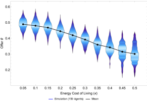
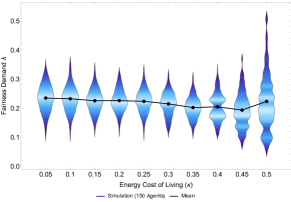
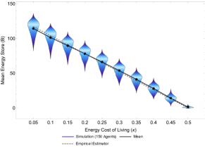
Figure 1: Simulation results using 150 agents, 300 rounds of play, and 100 replications: (top) there is a well defined negative correlation between cost of living and offer; (middle) Fairness demands are stable across cost of living values; (bottom) energy cache values follow an empirical trend derivable from the model.

Density plots showing the joint converged ($\theta$, $\lambda$) distributions are shown in Fig. 3. The convergence of $\theta^{i}(t)$ and $\lambda^{i}(t)$ is illustrated in Fig. 2 for $300$ agents, $T=500$ and $\kappa=0.1$. To create this figure, 100 replications were constructed and $\theta^{i}(t)$ and $\lambda^{i}(t)$ were sorted at each round. These sorted lists where then averaged (over replication) to obtain $\bar{\theta}^{[i]}(t)$ and $\bar{\lambda}^{[i]}(t)$, where $\bar{\theta}^{[i]}(t)$ is the mean offer value of the agent with the $i^{\text{th}}$ smallest offer value. The quantity $\bar{\lambda}^{[i]}(t)$ is defined analogously.

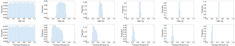
Figure 2: (top) Convergence of the distribution of $\theta^{i}$ from a uniform distribution to a delta distribution. (bottom) Convergence of the distribution of $\lambda^{i}$ from a uniform distribution to a delta distribution. (both) $\kappa=0.1$, 300 agents are simulated. Times go from $t=0$ to $t=500$ in increments of $\Delta t=100$.

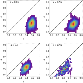
Figure 3: Density plots show the distributions of $(\theta^{*},\lambda^{*})$ over multiple replications with varying costs of living.

The simulation shows downward pressure on the offer value correlated with the energy cost of living $\kappa$ with consistent values of $\lambda^{*}$ between (approximately) $0.1$ and $0.4$. As is expected, the value of $\hat{B}^{i}(t)$, the mean energy store value decreases as a function of cost of living. We derive an empirical linear approximation for the mean, which we discuss in the sequel. Understanding the origin of this relationship is complicated by the fact that there is no convenience closed form expression for $\lambda^{i}(t)$ or $\theta^{i}(t)$. To remedy this, we use a combination of empirical distribution modeling and closed form analysis of $\Delta\hat{B}^{i}$ to explain the observed behavior.

3.1 Mixed Empirical and Closed form System Modeling

At arbitrary time $t$ when the distribution of fairness demands and offers is given by probability density functions $f^{t}_{\lambda}(s)$ and $f^{t}_{\theta}(s)$ respectively, then Eq. 8 can be generalized as:

$$\Delta\hat{B}(t;\theta,\lambda,\kappa)=\frac{1}{2}\left(\int_{0}^{\theta}(1-\theta)f_{\lambda}^{t}(s)\,ds+\int_{\lambda}^{1}sf_{\theta}^{t}(s)\,ds\right)-\kappa$$ (9)

This expression cannot be computed without the time-varying distributions in question, which cannot be computed without an appropriate Fokker-Plank equation, which is difficult to construct. To compensate, we can fit distributions to the data $\bar{\lambda}^{[i]}(t)$ and $\bar{\theta}^{[i]}(t)$ to obtain estimators $\hat{f}^{t}_{\lambda}(s)$ and $\hat{f}^{t}_{\theta}(s)$, which can be used in Eq. 9. These empirically estimated distributions stand in for the mean-field distributions. Not: All distributions were estimated using Mathematica’s FindDistribution function. We can then compute:

$$\hat{B}(t;\theta,\lambda,\kappa)=\begin{cases}B_{0}&\text{if t = 0}\\ \sum_{s\leq t}\Delta{B}(t;\theta,\lambda,\kappa)U[B(t-1;\theta,\lambda,\kappa)]&\text{otherwise}\end{cases},$$ (10)

where the factor $U[B(t-1;\theta,\lambda,\kappa)]$ sets $\hat{B}(t;\theta,\lambda,\kappa)=0$ if $\hat{B}(t-1;\theta,\lambda,\kappa)=0$. That is, it models the death of a test agent with parameters $(\theta,\lambda)$. The imitation dynamics defined by Eqs. 4, 5 and 7 imply that the larger $\hat{B}(t;\theta,\lambda,\kappa)$ the more likely an agent with parameters $(\theta,\lambda)$ will be imitated. Thus, we can use $\hat{B}(t;\theta,\lambda,\kappa)$ at an appropriately large time (e.g., $t=100$) to estimate which agents are most likely to be imitated for a given $\kappa$. We show this estimation for $\kappa=0.1$ and $\kappa=0.4$ in Fig. 4.

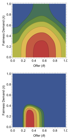
Figure 4: (top) (bottom)

To test this model, we use the top 5% of computed values of $\hat{B}(t,\theta,\lambda,\kappa)$ to compute estimated intervals on the values of $\theta^{*}$ and $\lambda^{*}$ for $\kappa=0.1$ and $\kappa=0.4$. We compare these intervals with the $5\%-95\%$ intervals computed from the experimental results shown in Fig. 1. This is shown in Table 1.

$\kappa$	Model Est. Interval	Computed Interval
$0.1$	$[0.43,0.64]$	[0.42,0.54]
$0.4$	$[0.25,0.41]$	[0.280.41]

Offer Estimate

$\kappa$	Model Est. Interval	Computed Interval
$0.1$	$[0,0.33]$	[0.15,0.31]
$0.4$	$[0,0.26]$	[0.13,0.28]

Fairness Demand Estimate

Table 1: Comparison of estimated and computed intervals on $\theta^{*}$ and $\lambda^{*}$ using information from Eq. 10.

These results are both consistent with and predictive of the distributions seen in Fig. 1; i.e., they explains both the downward slope of $\theta$ as a function of $\kappa$ in Fig. 1 (top) and the relatively constant behavior of $\lambda$ as a function of $\kappa$. We stress that estimations in Fig. 4 and Table 1 are generated by a model (Eq. 9 and Eq. 10) with distribution constants determined empirically. Thus an area of future work is to replace these empirically determined distributions with modeled distributions.

3.2 Asymptotic Behavior of $\hat{B}$

The dynamics of the energy cache values can be modeled asymptotically. As $t\to\infty$, $f^{t}_{\lambda}(s)\approx\delta(s-\lambda^{*})$ and $f^{t}_{\theta}(s)\approx\delta(s-\theta^{*})$, where $(\theta^{*},\lambda^{*})$ is the fixed point of the $(\theta(t),\lambda(t))$. This is illustrated in Fig. 2. As $t\to\infty$, the energy caches of each agent asymptotically approaches:

$$B^{i}(t)=(\tfrac{1}{2}-\kappa)t.$$

This model is shown in Fig. 1 (bottom). This over-estimates the long-run energy cache value because of the initial time taken to converge. We can approximate the trend seen in Fig. 1 (bottom), by noting that the time for $\lambda^{i}(t)$ and $\theta^{i}(t)$ to converge so that most UG interactions are successful in approximately 80 rounds (out of the 300 rounds simulated). Assuming that prior to convergence, only half of all interactions result in a successful UG, we obtain a thermodynamic-type relationship between the mean wealth of the population and the cost of living:

$$\tilde{B}(\kappa)=260\left(\frac{1}{2}-\kappa\right),$$ (11)

which explains the linear decrease with $\kappa$ shown in Fig. 1 (bottom), where we show the fit of Eq. 11.

Figure 5 shows the a log-plot of mean deaths per capita per simulation with notional cubic fit. As expected, there is a non-linear jump for $\kappa=\tfrac{1}{2}$. In addition, we note tht the zero-crossing (corresponding to one death per round) occurs roughly at $\kappa=\kappa^{*}$, representing a transition in the population to a more rapidly increasing per capita death rate with cost of living $\kappa$. This also correlates with more than 50% of the agents having initially decreasing energy caches, thus increasing the per capita death rate.

Figure 5: Log-Log plot of per capita death rate in the simulation as a function of energy cost of living.

The global dynamics displayed in Fig. 1 are robust to changes in the speed of the underlying dynamics. In particular, we tested models in which (i) we replaced the discrete dynamics with continuous time differential equations (by letting $\epsilon\to 0$), (ii) an Euler step approximation of the resulting differential equations and (iii) a heterogenous starting energy cache value with the previously described dynamics. The ODE variants model fast imitation (on the time scale of the game play). In all cases except one, we included reproduction as a hybrid step by solving the ODEs for short time horizons, checking for death and then restarting the ODEs from the previous condition after removing agents with $B^{k}<0$. All models used 100 replications except when reproduction was eliminated in which case 200 replications were used to ensure statistically signifiant sample sizes. (Samples with population collapse were discarded.)

Results from robustness experiments are shown in Fig. 6 (top), where we show the mean values $\bar{\theta}^{*}$. The envelopes are $1\sigma$. Similar tests were run for $\bar{\lambda}^{*}$ – see Fig. 6 (middle).

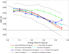
(a) Offer

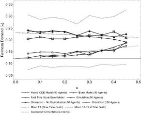
(b) Fairness Demand

Figure 6: (top) Model variations show the same trend in offer as a function of cost of living. (middle) Model variations show differing trend in fairness demand depending on imitation speed. (bottom) Scaling GDP as a proxy for cost of living in real-world data shows good correlation with the proposed model (number in parentheses denotes the number of countries averaged in each data point [16]).

For all cases, $\bar{\theta}$ is decreasing in $\kappa$. The mean fit line has negative slope as a function of $\kappa$ ($p=5.1\times 10^{-6}$) and adjusted $r^{2}$ of $0.95$, consistent with prior results and theoretical analysis. There is a difference in the behavior of $\bar{\lambda}^{*}$ for the the discrete time simulations and the continuous time (hybrid) variations. In the case of the hybrid ODE models (with or without Euler step approximations) $\bar{\lambda}^{*}$ increases as a function of $\kappa$ ($p<0.002$) while for discrete step simulations $\bar{\lambda}^{*}$ decreases as a function of $\kappa$ ($p<0.002$). When the data are combined, $\bar{\lambda}^{*}$ increases as a function of $\kappa$ but with $p<0.004$, suggesting this effect may disappear with larger samples. This would be the expected behavior as indicated by Fig. 4.

4 Discussion

The proposed model provides behavior consistent with observations in the meta-study by Oosterbeek et al. [16] insofar as a diversity of offer proportions and rejection rates are shown to be possible as a result of random interaction and imitation of multiple agents. Over all simulations, the grand mean $\langle{\theta}\rangle=0.43\pm 0.00032$, which is consistent with the $40.41\%$ offer rate observed in [16]. The grand mean $\langle{\lambda}\rangle=0.20\pm 0.00026$, implying that $20\%$ of offers would be rejected if chosen uniformly randomly from $[0,1]$. [16] reports a mean rejection rate of $16\%$, which is consistent with the results produced by the model assuming some cultural learning (imitation) has occurred. As noted, the distributions describing $\lambda^{*}$ have ranges from approximately $0.1$ to $0.4$, adequately modeling the large variation in rejection rates. Despite these similarities, we cannot fully validate the model empirically because neither [16] nor its constituent studies include a variable like cost of living. Their study does regress against GDP and reward as a percent of per capita GDP (which spans 2 orders of magnitude), but this is not an accurate measurement of intrinsic cost of living, especially in geographically diverse areas like the United States. We note that in [16], regression of offer against GDP shows an insignificant negative correlation, which is consistent with Fig. 1 and Fig. 6 (top), but these studies were not designed to measure this relationship. The results of this study suggest potential experimental analysis that could be done in controlled laboratory settings.

5 Conclusion

Game Theory finds application in biological and social sciences, yet well-known occurrences like cooperation and altruism remain challenging within its rational self-interest assumptions. Our paper presents a novel approach to the canonical Ultimatum Game (UG), introducing an additional savings variable (energy) along with a cost of living. In our nonlinear agent-based model, energy represents success and drives imitation. Agents evolve toward fair sharing, but are more selfish with higher costs of living, with consistently lower fairness demands of others. This behavior is explained and predicted using a model with empirical determined distribution parameters. The model reproduces some empirical data of human UG performance across cultures, providing a new theoretical framework for heterogenous cooperation among humans. In future work, we will explore these dynamics further to determine whether the exact structure of the distributions on $\theta$ and $\lambda$ can be determined. This would remove the need to fit the distributions as a part of the modeling process and provide a complete mean-field dynamics for this system.

References

- [1] Robert Axelrod. The emergence of cooperation among egoists. American Political Science Review, 75(2):306–318, 1981.
- [2] Damien Challet and Y-C Zhang. Emergence of cooperation and organization in an evolutionary game. Physica A: Statistical Mechanics and its Applications, 246(3-4):407–418, 1997.
- [3] Sanjay Jain and Sandeep Krishna. A model for the emergence of cooperation, interdependence, and structure in evolving networks. Proceedings of the National Academy of Sciences, 98(2):543–547, 2001.
- [4] Martin A Nowak, Akira Sasaki, Christine Taylor, and Drew Fudenberg. Emergence of cooperation and evolutionary stability in finite populations. Nature, 428(6983):646–650, 2004.
- [5] Francisco C Santos and Jorge M Pacheco. Scale-free networks provide a unifying framework for the emergence of cooperation. Physical Review Letters, 95(9):098104, 2005.
- [6] Daniel J Hruschka and Joseph Henrich. Friendship, cliquishness, and the emergence of cooperation. Journal of theoretical biology, 239(1):1–15, 2006.
- [7] Francisco C Santos, Marta D Santos, and Jorge M Pacheco. Social diversity promotes the emergence of cooperation in public goods games. Nature, 454(7201):213–216, 2008.
- [8] Shun Kurokawa and Yasuo Ihara. Emergence of cooperation in public goods games. Proceedings of the Royal Society B: Biological Sciences, 276(1660):1379–1384, 2009.
- [9] Sven Van Segbroeck, Jorge M Pacheco, Tom Lenaerts, and Francisco C Santos. Emergence of fairness in repeated group interactions. Physical Review Letters, 108(15):158104, 2012.
- [10] Elisabeth Paulson and Christopher Griffin. Cooperation can emerge in prisoner’s dilemma from a multi-species predator prey replicator dynamic. Mathematical biosciences, 278:56–62, 2016.
- [11] Pengbi Cui, Zhi-Xi Wu, Tao Zhou, Xiaojie Chen, et al. Cooperator-driven and defector-driven punishments: How do they influence cooperation? Physical Review E, 100(5):052304, 2019.
- [12] Shiping Gao, Jinming Du, and Jinling Liang. Evolution of cooperation under punishment. Physical Review E, 101(6):062419, 2020.
- [13] John Gale, Kenneth G. Binmore, and Larry Samuelson. Learning to be imperfect: The ultimatum game. Games and Economic Behavior, 8(1):56 – 90, 1995.
- [14] Gary Bornstein and Ilan Yaniv. Individual and group behavior in the ultimatum game: Are groups more “rational” players? Experimental Economics, 1(1):101–108, Jun 1998.
- [15] Alan G. Sanfey, James K. Rilling, Jessica A. Aronson, Leigh E. Nystrom, and Jonathan D. Cohen. The neural basis of economic decision-making in the ultimatum game. Science, 300(5626):1755–1758, 2003.
- [16] H. Oosterbeek, R. Sloof, and G. Van De Kuilen. Cultural differences in ultimatum game experiments: Evidence from a meta-analysis. Experimental Economics, 7:171–188, 2004.
- [17] Kevin J. Haley and Daniel M.T. Fessler. Nobody’s watching?: Subtle cues affect generosity in an anonymous economic game. Evolution and Human Behavior, 26(3):245 – 256, 2005.
- [18] Joseph Henrich, Richard McElreath, Abigail Barr, Jean Ensminger, Clark Barrett, Alexander Bolyanatz, Juan Camilo Cardenas, Michael Gurven, Edwins Gwako, Natalie Henrich, Carolyn Lesorogol, Frank Marlowe, David Tracer, and John Ziker. Costly punishment across human societies. Science, 312(5781):1767–1770, 2006.
- [19] Keith Jensen, Josep Call, and Michael Tomasello. Chimpanzees are rational maximizers in an ultimatum game. Science, 318(5847):107–109, 2007.
- [20] Toshio Yamagishi, Yutaka Horita, Haruto Takagishi, Mizuho Shinada, Shigehito Tanida, and Karen S. Cook. The private rejection of unfair offers and emotional commitment. Proceedings of the National Academy of Sciences, 106(28):11520–11523, 2009.
- [21] Terence Burnham. Gender, Punishment, and Cooperation: Men Hurt Others to Advance Their Interests. Available at SSRN: https://papers.ssrn.com/soL3/papers.cfm?abstract_id=2966376, 2017.
- [22] Björn Wallace, David Cesarini, Paul Lichtenstein, and Magnus Johannesson. Heritability of ultimatum game responder behavior. Proceedings of the National Academy of Sciences, 104(40):15631–15634, 2007.
- [23] David Cesarini, Christopher T. Dawes, James H. Fowler, Magnus Johannesson, Paul Lichtenstein, and Björn Wallace. Heritability of cooperative behavior in the trust game. Proceedings of the National Academy of Sciences, 105(10):3721–3726, 2008.
- [24] Katherine A. Cronin, Daniel J. Acheson, Penélope Hernández, and Angel Sánchez. Hierarchy is detrimental for human cooperation. Scientific Reports, 5:18634 EP –, 12 2015.
- [25] Martin A. Nowak, Karen M. Page, and Karl Sigmund. Fairness versus reason in the ultimatum game. Science, 289(5485):1773–1775, 2000.
- [26] David G. Rand, Corina E. Tarnita, Hisashi Ohtsuki, and Martin A. Nowak. Evolution of fairness in the one-shot anonymous ultimatum game. Proceedings of the National Academy of Sciences, 110(7):2581–2586, 2013.
- [27] Karen M Page, Martin A Nowak, and Karl Sigmund. The spatial ultimatum game. Proceedings of the Royal Society of London B: Biological Sciences, 267(1458):2177–2182, 2000.
- [28] Karen M. Page and Martin A. Nowak. A generalized adaptive dynamics framework can describe the evolutionary ultimatum game. Journal of Theoretical Biology, 209(2):173 – 179, 2001.
- [29] M. N. Kuperman and S. Risau-Gusman. The effect of the topology on the spatial ultimatum game. The European Physical Journal B, 62(2):233–238, Mar 2008.
- [30] Jaime Iranzo, Javier Román, and Angel Sánchez. The spatial ultimatum game revisited. Journal of Theoretical Biology, 278(1):1 – 10, 2011.
- [31] Q. Zhu, S. Rajtmajer, and A. Belmonte. The emergence of fairness in an agent-based ultimatum game. working paper, 2016.
- [32] Sarah Rajtmajer, Anna Squicciarini, Jose M Such, Justin Semonsen, and Andrew Belmonte. An ultimatum game model for the evolution of privacy in jointly managed content. In International Conference on Decision and Game Theory for Security, pages 112–130. Springer, 2017.
- [33] Bruce M Boghosian. Kinetics of wealth and the pareto law. Physical Review E, 89(4):042804, 2014.
- [34] Nicola McGuigan. The influence of model status on the tendency of young children to over-imitate. Journal of experimental child psychology, 116(4):962–969, 2013.
- [35] Harriet Over and Malinda Carpenter. Children infer affiliative and status relations from watching others imitate. Developmental science, 18(6):917–925, 2015.
- [36] Jelena Grujić and Tom Lenaerts. Do people imitate when making decisions? evidence from a spatial prisoner’s dilemma experiment. Royal Society Open Science, 7(7):200618, 2020.
- [37] Christopher Griffin, Sarah Rajtmajer, Anna Squicciarini, and Andrew Belmonte. Consensus and information cascades in game-theoretic imitation dynamics with static and dynamic network topologies. SIAM Journal on Applied Dynamical Systems, 18(2):597–628, 2019.
- [38] S. Motsch and E. Tadmor. Heterophilious Dynamics Enhances Consensus. SIAM Review, 56:577–621, 2014.