Compression-aware Continual Learning using Singular Value Decomposition

Abstract

We propose a compression based continual task learning method that can dynamically grow a neural network. Inspired from the recent model compression techniques, we employ compression-aware training and perform low-rank weight approximations using singular value decomposition (SVD) to achieve network compaction. By encouraging the network to learn low-rank weight filters, our method achieves compressed representations with minimal performance degradation without the need for costly fine-tuning. Specifically, we decompose the weight filters using SVD and train the network on incremental tasks in its factorized form. Such a factorization allows us to directly impose sparsity-inducing regularizers over the singular values and allows us to use fewer number of parameters for each task. We further introduce a novel shared representational space based learning between tasks. This promotes the incoming tasks to only learn residual task-specific information on top of the previously learnt weight filters and greatly helps in learning under fixed capacity constraints. Our method significantly outperforms prior continual learning approaches on three benchmark datasets, demonstrating accuracy improvements of 10.3%, 12.3%, 15.6% on 20-split CIFAR-100, miniImageNet and a 5-sequence dataset, respectively, over state-of-the-art. Further, our method yields compressed models that have $\sim 3.64\times,2.88\times,5.91\times$ fewer number of parameters respectively, on the above mentioned datasets in comparison to baseline individual task models. Our source code is available at https://github.com/pavanteja295/CACL.

1 Introduction

The ability to learn novel information without interfering with the consolidated previous knowledge is referred to as life-long or continual learning. Deep learning methods have demonstrated superseding performances and improvements on single-task learning [22] and multi-task learning [38] that aims to jointly optimize over several tasks at once. Albeit this success, neural networks suffer from catastrophic forgetting during sequential-task learning and lack the ability to incrementally learn new information. This is ascribed to the representational overlap between tasks resulting in interference of new information with previous knowledge [12].

Recent studies have proposed methods that alleviate the catastrophic forgetting problem. Some approaches referred to as regularization based methods estimate the contribution of the individual parameters in a network to prior tasks and regularize the weight changes/updates based on the estimated importance while training new tasks [3, 20, 37, 31]. However, these methods assume fixed network capacity that upper bounds the number of tasks that can be learnt. In fact, the authors in [14] observed degrading performance of such approaches over longer task sequences. Other line of work categorized as memory-replay methods [8, 24, 28, 6] retain examples from previous tasks to retrain the network that helps restore performances on old tasks. But these methods are burdened with retraining on all previous tasks for every new task.

Network expansion methods consider growing the network to avoid the representational overlap between tasks and accommodate unlimited number of tasks. Further, some of these approaches [30, 25, 26, 15] guarantee preservation of performances on previous tasks and eliminate retraining on old tasks. Nevertheless, unrestricted growing of networks is computationally expensive and memory intensive that hinders their real-time implementation on hardware with limited memory. Approaches like [16, 25, 15, 2] employ pruning procedures to achieve network compaction, thereby, reducing the memory consumption. However, such pruning procedures are either iterative and gradual or require an additional fine-tuning/retraining step to restore the performance. Other works [36, 15] control the model growth by introducing carefully designed expansion schemes that are time-consuming.

In this paper, we propose a network expansion method for continual learning addressing the above mentioned weaknesses while demonstrating significant improvements to average performance and model compaction. By adopting two main characteristics: 1) Network Factorization, and 2) Additive Shared Representational Space, we achieve state-of-the results with best model compression rates on three benchmark datasets. Our compression step produces compact representations in oneshot for each task with minimal performance degradation unlike the iterative and time-consuming pruning strategies used in prior works. Our compression technique is inspired from the recent low-rank approximation methods [9, 4, 2] using SVD that compress networks via singular value pruning. We resort to compression-aware training by encouraging the model to learn low-rank weight filters by enforcing sparsity regularizers over singular values similar to [35, 4, 34]. This minimizes the performance degradation during the compression step eliminating the costly retraining. Moreover, we achieve maximal compression with a novel additive shared representation learning between tasks. Our proposed sharing technique enables adding residual task-specific information pertaining to the incoming tasks on the already learnt weight filters from prior tasks. We employ a simple unconstrained expansion scheme to accommodate new incoming tasks.

To summarize, our contributions are:

• We propose a simple yet effective incremental task learning algorithm that does not resort to time-consuming intermediate heuristics.

• We employ compression-aware training of neural networks in the SVD decomposed form to tackle sequential task learning. We compress the trained task representations using low-rank approximations and incorporate incoming tasks by expansion.

• We propose additive shared representations between tasks in the factorized space that encourages the incoming tasks to learn task-specific information.

• We show significant improvements in performance over state-of-the-art approaches on benchmark datasets, CIFAR100 [21], miniImageNet [33] and 5-sequence dataset [11] with much smaller model size. Through a fair comparison with other network-based expansion methods, we show that our approach is highly optimal by remarkably outperforming in accuracy and compression.

2 Related Work

Regularization based methods control the updates to the weights based on their degree of importance per task. EWC [20] identifies significant weights by using Fischer Information Matrix, while authors in [37] estimate importance of parameters by their individual contribution over the entire loss trajectory. Improvements to efficiency and memory consumption of EWC was proposed in [5]. HAT [31] proposes to learn attention mask to control the weight updates while training on new tasks. The authors in [10] employ a Bayesian framework where, parameters predicted with high certainty are considered crucial to maintain previous task performance.

Memory replay methods deal with the catastrophic forgetting of previous experiences by rehearsing the old tasks while training the new tasks. This is achieved by either storing subset of data [24, 7, 29, 6, 8] from previous tasks or by synthesizing the old data using generative models [19, 32]. Sample selection strategy plays an important role in these approaches due to the limited computational budget. Significant improvements in performance were demonstrated by [8, 27] by employing reservoir sampling than random sampling for selecting examples from old tasks.

Network expansion methods increases the network capacity to prevent interference among task representations during incremental task learning. Our work largely belongs to this line of work. ProgressiveNet [30] accommodates new tasks by instantiating a new network for each task but at the cost of linear architectural growth. To avoid this, the authors in [36] allow network expansion only when required based on the task relatedness to the previous knowledge. PiggyBack [26] learns a selection mask per task to adapt a fixed backbone network to multiple tasks and requires a pre-trained backbone. In contrast to PiggyBack, our method can continually learn from scratch. Our approach is closely related to [15, 16] that follow a learn-compress-grow cycle for each task. However, the above methods use gradual pruning and compression schemes that are time-consuming. Another recent work [2] also focuses on compression for continual learning tasks. The authors in [2] use Principal Component Analysis[1] on the feature maps to detect the relevant task-specific filters and remove redundant filters while learning tasks sequentially. However, they perform compression across channels of different layers and do not preserve the initial network design unlike our approach. Furthermore, the authors in [2] train the network in a generic manner and then use PCA to determine the optimal task-specific filters to prune/retain. Then, they employ a fine-tuning/re-training step after every compression step to recover the performance degradation due to compression. In contrast to [2], the novelty of our method is that we train the network in the SVD factorized space that encourages low-rank approximation and sparsification. This SVD space continual training provides us with the advantage of eliminating the re-training step while achieving maximal compression without any significant performance loss.

Low rank approximation: Recent works [9, 18] demonstrated significant model compression rates using low-rank approximations of the weights of a network. To minimize loss in accuracy due to the compression, the authors in [4, 34, 35] propose embedding low-rank decomposition during training by imposing sparsity over the singular values to learn low-rank weight filters.

3 Compression-aware Continual Learning (CACL)

We consider the problem of incremental task learning where, $T$ tasks with unknown data-distributions are to be learnt in a sequence with the help of training data $\mathcal{D}_{t}$ where $\mathcal{D}_{t}$ = $\{x_{i},y_{i}\}_{i=1}^{N_{t}}$ and $t\in\{1,2,...T\}$. In the sections below, we discuss the steps for our proposed CACL methodology. An overview of CACL is outlined in Fig. 1 and Algorithm 2. In essence, for any incoming task $t$, we instantiate a convolutional network in SVD parameterized form (Section 3.4). We train the factorized network by incorporating sharing between tasks (Section 3.3) and impose sparsity-inducing regularizer to encourage low-rank weight solutions (Section 3.5). We finally compress the task representations using low rank approximations of the weight filters and update the shared space by appending the compressed representations (Section 3.6).

3.1 Background

Singular Value Decomposition: SVD factorization of any real 2-dimensional matrix $\mathcal{A}$ $\in$ $R^{m\times n}$ is given by $Udiag(\sigma)V^{T}$ where $U$ $\in R^{m\times m}$, $V\in R^{n\times n}$, $diag(\sigma)$ $\in$ $R^{m\times n}$ are left singular vectors, right singular vectors, diagonal matrix with singular values on the principal diagonal, respectively. By construction, $U^{T}U=UU^{T}=I$ , $V^{T}V=VV^{T}=I$. One could consider a reduced SVD form by only retaining the non-zero singular values and their corresponding singular vector columns. Then $\mathcal{A}$ can be safely factorized into $U$ $\in R^{m\times r}$, $V\in R^{n\times r}$, $diag(\sigma)$ $\in$ $R^{r\times r}$. Dimension $r$ refers to the rank of the matrix which is the number of non-zero singular values. We refer to reduced SVD as SVD in the subsequent sections.

Rank-k approximation: For any real matrix $\mathcal{A}$ $\in$ $R^{m\times n}$ and $m\geq n$, the best rank-k approximation is given by $\mathcal{A}_{k}=\sum_{i=1}^{k}\sigma_{i}u_{i}v_{i}^{T}$ where, $\sigma_{1}\geq\sigma_{2}...\geq\sigma_{n}\geq 0$ are the sorted singular values. Here, $u_{i}\in$ $R^{m\times 1}$, $v_{i}$ $\in$ $R^{n\times 1}$ denote the corresponding left and right singular columns from $U$ and $V$, respectively. Rank-k approximation using SVD essentially prunes the insignificant singular values ($k+1$ to $n$) and their corresponding singular vectors which ultimately enables compression in our approach. However, such an approximation introduces error. The Frobenius norm due to the substitution of $\mathcal{A}$ with $\mathcal{A}_{k}$ is given as $\lVert\mathcal{A}-\mathcal{A}_{k}\rVert_{F}=\sum_{i=k+1}^{n}\sigma^{2}_{i}$ where, $\lVert.\rVert_{F}$ represents the Frobenius norm. The difference between $\mathcal{A}$ and $\mathcal{A}_{k}$ is highly minimized when $\mathcal{A}$ is sufficiently low-rank. Thus, we encourage the model to learn low-rank weight filters during training by imposing sparsity-inducing regularizer over singular values.

Notations: For convenience, we provide the reader the notations used in the subsequent sections and their definitions. $\mathcal{W}^{t}=\{W^{t}_{l}\}^{L}_{l=1}$ represents the weight tensors of a neural network for task $t$ across all layers where, $W^{t}_{l}$ corresponds to the weight tensor of task $t$ at layer $l$. Similarly, we denote $\mathcal{U}^{t}=\{U^{t}_{l}\}_{l=1}^{L}$, $\mathcal{V}^{t}=\{V^{t}_{l}\}_{l=1}^{L}$, $\mathcal{S}^{t}=\{S^{t}_{l}\}_{l=1}^{L}=\{diag(\sigma)^{t}_{l}\}_{l=1}^{L}$. $U^{t}_{l}$, $V^{t}_{l}$ denotes the left and right singular vectors, while $S^{t}_{l}$ or $diag(\sigma)^{t}_{l}$ denotes the diagonal matrix with singular values on the principal diagonal. $\sigma^{t}_{l}$ denotes the singular values in vectorized form. We consider $\mathcal{U}^{t},\mathcal{V}^{t},\mathcal{S}^{t}$ to be the left singular vectors, right singular vectors, singular values, respectively, across all layers for task $t$. Any operation on $\mathcal{U}^{t},\mathcal{V}^{t},\mathcal{S}^{t}$ unless otherwise specified is meant to be applied for each layer separately.

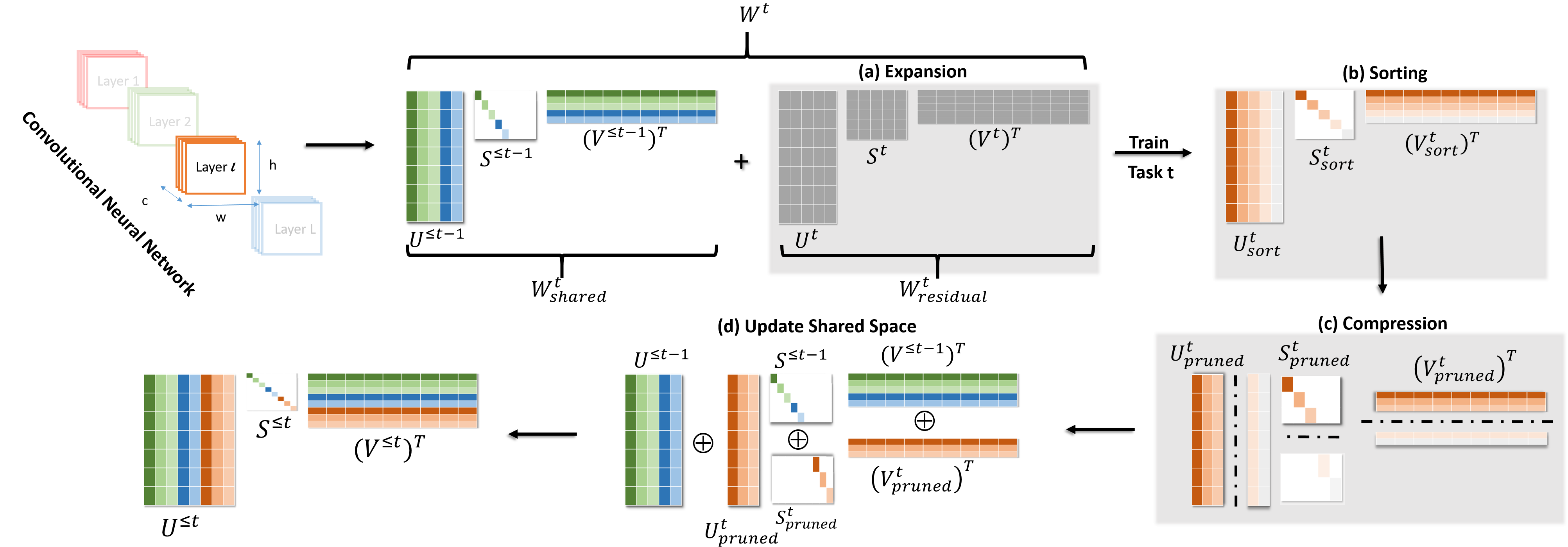
Figure 1: A schematic of CACL training pipeline for a layer $l$ and task $t$ is shown. For simplicity, we drop the notation ‘$l$’ from all the parameters. (a) We start with expansion by creating randomly initialized trainable parameters $U^{t},V^{t},S^{t}$. We then train the parameters $U^{t},V^{t},S^{t}$ following Section 3.5. (b) We obtain the sorted singular values and vectors $U^{t}_{sort},V^{t}_{sort},S^{t}_{sort}$ by performing sorting on the singular values after training. (c) We apply our compression step as discussed in Section 3.6 that results in $U^{t}_{pruned},V^{t}_{pruned},S^{t}_{pruned}$. (d) Finally, the compressed singular values and vectors are added to shared space that returns the $U^{\leq t},V^{\leq t},S^{\leq t}_{l}$ used by the next incoming task t+1.

3.2 Network Factorization

Our motivation to train and store the learnt representations of a neural network in the factorized SVD form is drawn from two advantages. Firstly, it allows preserving the low-rank weight filters with fewer number of parameters. For a convolutional layer $W_{conv}\in R^{c\times n\times h\times w}$ where $c$ is the number of output channels, $h\times w$ is size of the kernel, $n$ is the number of input channels, the number of parameters required to store a 4D weight matrix is cnhw. However, when $W_{conv}$ is sufficiently low-rank, this representation could be sub-optimal. Thus, we reshape the 4D tensor to a 2D matrix and decompose the matrix using SVD into $U_{conv}$ $\in$ $R^{c\times r}$, $V_{conv}$ $\in$ $R^{nhw\times r}$, $diag(\sigma)_{conv}$ $\in$ $R^{r\times r}$. The SVD parameterized form requires cr + nhwr + r parameters. For $r<<\frac{cnhw}{c+nhw+1}$, the factorized representation significantly reduces the memory consumption compared to original representation. Secondly, one can directly impose sparsity regularizers over the singular values to promote learning low-rank filters, without resorting to costly SVD factorization at every training step.

We maintain the factorized form throughout the training as well as inference that adds a small computational overhead to construct the 4D convolutional weight filters from the decomposed parameters. As a result for any task $t$, our trainable parameters are $\mathcal{U}^{t},\mathcal{V}^{t},\mathcal{S}^{t}$. Note that, such a factorization does not mutate the architecture of the network, but rather modifies the representations we learn and store.

3.3 Shared Representational Space

For any incoming task $t$, we reuse the previously accumulated experiences from old tasks and promote tasks to learn on top of the previous weight filters. This encourages learning task-specific residual information. We introduce a novel sharing scheme in the factorized space that allows incoming tasks to leverage previous knowledge. This is enabled by constructing the 2D reshaped (reshaping 4D tensor to 2D matrix as explained in Section 3.2) convolutional weight filters while training a task $t$ as below:

$$\mathcal{W}^{t}=\underset{\text{Frozen}}{\boxed{\mathcal{U}^{\leq t-1}\mathcal{S}^{\leq t-1}(\mathcal{V}^{\leq t-1})^{T}}}+\underset{\text{Trainable}}{\boxed{\mathcal{U}^{t}\mathcal{S}^{t}(\mathcal{V}^{t})^{T}}}$$ (1)

where $+$ represents element-wise addition across all layers. As shown in Eqn. 1, during task $t$ training, the trainable parameters are $\mathcal{U}^{t},\mathcal{S}^{t},\mathcal{V}^{t}$, while $\mathcal{U}^{\leq t-1},\mathcal{S}^{\leq t-1},\mathcal{V}^{\leq t-1}$ are frozen. Intuitively, one can interpret our sharing mechanism as adding residual task related weight filters ($\mathcal{W}^{t}_{residual}$) to the previously learnt weights ($\mathcal{W}^{t}_{shared}$) where, $\mathcal{W}^{t}_{residual}=\mathcal{U}^{t}\mathcal{S}^{t}(\mathcal{V}^{t})^{T}$ and $\mathcal{W}^{t}_{shared}=\mathcal{U}^{\leq t-1}\mathcal{S}^{\leq t-1}(\mathcal{V}^{\leq t-1})^{T}$. Note, our sharing technique maintains the intended network design (number of layers or number of weight filters within each layer) unlike previous network expansion approaches [36, 15].

Input : Dataset $\mathcal{D}$ = ($D_{1},D_{2},...D_{T}$), $\mathcal{W}=\{W_{l}\}_{l=1}^{L}$, $Threshold=e$

$\mathcal{U}^{t=0},\mathcal{S}^{t=0},\mathcal{V}^{t=0}=[\;]$

  $\triangleright$ Intialization

for $t\leftarrow 1,2,...T$ do

       $\mathcal{U}^{t},\mathcal{S}^{t},\mathcal{V}^{t}=\;$Expansion ($\mathcal{W}$)

        $\triangleright$ Section 3.4

       $\mathcal{U}^{t},\mathcal{S}^{t},\mathcal{V}^{t}=\emph{TrainTask}(D_{t}$, $[\mathcal{U}^{\leq t-1},\mathcal{S}^{\leq t-1},\mathcal{V}^{\leq t-1}]$, $[\mathcal{U}^{t},\mathcal{S}^{t},\mathcal{V}^{t}]$)

        $\triangleright$ Section 3.5

       $\mathcal{U}^{t}_{pruned},\mathcal{S}^{t}_{pruned},\mathcal{V}^{t}_{pruned}=\;$Compression ( $[\mathcal{U}^{t},\mathcal{S}^{t},\mathcal{V}^{t}]$, $e$)

        $\triangleright$ Section 3.6

       $\mathcal{U}^{\leq t},\mathcal{S}^{\leq t},\mathcal{V}^{\leq t}=\;$ $\mathcal{U}^{\leq t-1}\bigoplus\mathcal{U}^{t}_{pruned},\;\mathcal{S}^{\leq t-1}\bigoplus\mathcal{S}^{t}_{pruned},\;\mathcal{V}^{\leq t-1}\bigoplus\mathcal{V}^{t}_{pruned}$

end for

Algorithm 1 Compression-aware Continual Learning (CACL)

3.4 Expansion

For any incoming task $t$, we create randomly initialized parameters namely, $\mathcal{U}^{t},\mathcal{S}^{t},\mathcal{V}^{t}$. Specifically, for each layer $l$ of a given network, we create trainable parameters $U^{t}_{l}\in R^{c\times r},V^{t}_{l}\in R^{nhw\times r},S^{t}_{l}\in R^{r\times r}$ that learns the task-specific residual information (See Fig. 1(a)). The dimensions $c,n,h,w$ denote the output channels, input channels, kernel height and kernel width of the weight filter in layer $l$ of the given network, respectively. The dimension $r$ of the instantiated matrices is equal to $r=\frac{cnhw}{c+nhw+1}$ to ensure the number of trainable parameters in the factorized network be same as the original network. We further create an individual task-head for task $t$ referred to as $T^{t}_{head}$ attached on top of the network that predicts the final task-specific output.

3.5 Compression-Aware Training

We learn task $t$ by training the parameters $\mathcal{U}^{t},\mathcal{S}^{t},\mathcal{V}^{t},T^{t}_{head}$ created during the expansion step using the task $t$ dataset $D_{t}=\{x_{i},y_{i}\}_{i=1}^{N_{t}}$. The convolutional weight filters ($\mathcal{W}^{t}=\mathcal{W}^{t}_{shared}+\mathcal{W}^{t}_{residual}$) at every training step are constructed using the sharing technique (Eqn. 1) discussed in Section 3.3. Task $t$ is learnt by applying the task-specific loss function denoted as $\mathcal{L}_{task}$ on the task-head $T_{head}^{t}$. Throughout the training, we ensure $\mathcal{W}^{t}_{residual}$ maintains a valid SVD form so that we can obtain the best low-rank approximations during our compression step (see Section 3.1). For this, we require parameters $\mathcal{U}^{t},\mathcal{V}^{t}$ to be orthogonal i.e. $\mathcal{U{U}}^{T}=\mathcal{U}^{T}\mathcal{U}=I$ and $\mathcal{V{V}}^{T}=\mathcal{V}^{T}\mathcal{V}=I$. Hence, we employ an orthogonality-regularizer ($\mathcal{L}_{orth}$) proposed in [35] on parameters $\mathcal{U}^{t},\mathcal{V}^{t}$ which is given by: $\mathcal{L}_{orth}=\sum_{l=1}^{L}\dfrac{1}{r^{2}}(\lVert(U^{t}_{l})^{T}U^{t}_{l}-I\rVert_{F}+\lVert(V^{t}_{l})^{T}V^{t}_{l}-I\rVert_{F})$ where, $\lVert.\rVert_{F}$ is the Frobenius norm, $I$ is the identity matrix, $r$ refers to the rank of the parameters $U^{t}_{l}$ and $V^{t}_{l}$.

Note, low-rank approximations of the weight filters could introduce errors that can cause severe performance degradation during the compression phase (See Section3.1). This degradation can be minimized by learning low rank weight filters during training. To accomplish this, we impose sparsity-inducing regularizer over the singular values during training. We employ Hoyer regularization [35] that was observed to achieve better singular value sparsity than others (such as $L_{1}$ and $L_{2}$ norms). We denote the Hoyer regularization term as $\mathcal{L}_{sparse}$ where, $\mathcal{L}_{sparse}=\sum_{l=1}^{L}\dfrac{\lVert\sigma^{t}_{l}\rVert_{1}}{\lVert\sigma^{t}_{l}\rVert_{2}}$. $\lVert.\rVert_{1}$ denotes the $L_{1}$ norm and $\lVert.\rVert_{2}$ refers to the $L_{2}$ norm.

The overall loss function and the optimization objective while training a task $t$ corresponds to:

$$\begin{aligned} \mathcal{L}_{total}=\mathcal{L}_{task}+\lambda_{orth}\mathcal{L}_{orth}+\lambda_{sparse}\mathcal{L}_{sparse}\\ \underset{\mathcal{U}^{t},\mathcal{V}^{t},\mathcal{S}^{t}}{\text{minimize}}\quad\mathcal{L}_{total}(\mathcal{U}^{t},\mathcal{V}^{t},\mathcal{S}^{t}\textbf{;}\quad\mathcal{U}^{\leq t-1},\mathcal{S}^{\leq t-1},\mathcal{V}^{\leq t-1},\mathcal{D}_{t})\end{aligned}$$ (2)

where $\lambda_{orth},\lambda_{sparse}$ are the hyper-parameters to control the effect of each component and $D_{t}$ refers to the training data of task $t$. We provide the pseudo code of task training ($TrainTask$ function in Algorithm 1) in the supplementary material.

3.6 Compression

We obtain trained $\mathcal{U}^{t},\mathcal{S}^{t},\mathcal{V}^{t}$ parameters and perform singular value pruning at each layer l to achieve low-rank approximations of $\mathcal{W}_{residual}$. We initially sort the singular values in $\mathcal{S}^{t}$ and their corresponding singular vectors in descending order which returns $\mathcal{U}_{sort}^{t},{S}_{sort}^{t},{V}_{sort}^{t}$ (See Fig. 1(b)). We then retain only the top k highest singular values and their corresponding singular vectors eliminating the insignificant singular values. This results in the rank-k approximation of $\mathcal{W}_{residual}$ and outputs $\mathcal{U}_{pruned}^{t}{S}_{pruned}^{t},{V}_{pruned}^{t}$ with the rank of the parameters equal to $k$ (See Fig. 1c). The top $k$ value determines the number of singular values to retain. However, resorting to a constant $k$ for all the tasks and layers without task-consideration will be sub-optimal. Hence, we follow the below heuristic inspired from [34]. We prune the singular values based on total singular value energy which is given by, $\sum_{i=k+1}^{n}(\sigma_{i})^{2}\leq e\sum_{j=1}^{k}(\sigma_{j})^{2}$, where $e$ is a hyperparameter that controls the pruning intensity and $\sigma_{i},\sigma_{j}\in\sigma^{t}_{l}$. The above heuristic allows dynamic memory allocation to different tasks, that is a favourable characteristic in incremental task learning approaches. We provide a psuedo-code of our compression algorithm in the supplementary material.

Finally, compressed task representations $\mathcal{U}_{pruned}^{t},\mathcal{S}_{pruned}^{t},\mathcal{V}_{pruned}^{t}$ are appended to the existing shared space $\mathcal{U}^{\leq t-1},\mathcal{S}^{\leq t-1},\mathcal{V}^{\leq t-1}$ that results in a new shared space $\mathcal{U}^{\leq t},\mathcal{S}^{\leq t},\mathcal{V}^{\leq t}$. We store the rank of the parameters in the new shared space as task-identifiers for task $t$. During inference, we use the task-identifier of a task $t$ to extract the sub network $\mathcal{U}^{\leq t},\mathcal{S}^{\leq t},\mathcal{V}^{\leq t}$. For a $L$ layered neural network and $T$ tasks, storing the task-identifier incurs an overhead of $L\times T$ integer values.

4 Experiments

We evaluate our approach on three benchmark datasets - CIFAR-100[21], miniImageNet[33], 5-sequence dataset [11]. We follow the evaluation protocols proposed by recent works [11, 15] for a fair comparison with other approaches. We use a simple 5 layer convolutional neural network to demonstrate the effectiveness of our approach. We use a single hidden layer followed by softmax for each task as the task-head (${T^{t}}_{head}$) to output task specific classification scores. Unless explicitly mentioned, we use the above architecture for all our experiments. We refer the reader to supplementary section for the architectural details and hyperparameter configurations. Although our SVD factorization and compression-aware training approach can be extended to linear layers, in our experiments we apply it on convolutional layers. Our approach is referred as $CACL$ in the results.

We further train and evaluate a simple baseline that serves as the upper bound on the average performance for our approach. The baseline consists of individual single task models trained separately for each task using the above mentioned 5 layer convolutional network. We refer to this as Baseline_UB. All the results reported on our approach are averaged across 3 runs with random task ordering and weight initialization as prior works. We would further like to note that the overhead observed for training the 5 layer convolutional network in factorized form using CACL is marginal compared to standard training.

Evaluation metrics: We report the test classification accuracy averaged across all tasks abbreviated as ACC. We further report the size of the final trained models in Mega Bytes(assuming 32-bit floating point is equivalent to 4 bytes). We also report the backward transfer (BWT) introduced in [24], that denotes the average forgetting and the influence of learning new tasks on previous tasks. Lower BWT score implies better continual learning.

4.1 20-split CIFAR-100

We conduct two experiments on CIFAR-100 dataset, referred to as Protocol 1 and Protocol 2. For both protocols, we split CIFAR-100 dataset [21] into 20 disjoint tasks learning 5 class classification per task. We discuss below the motivation and the results obtained on each protocol using our method.

Protocol 1: In this protocol, we follow evaluation settings proposed by the recent continual learning methods [11, 6]. The focus of this experiment is to achieve the best performance and show the effectiveness of our CACL approach using a simple 5-layer convolutional network (mentioned above) without any additional components(such as residual connections [13], batch normalization [17]). Note, the results of the recent works reported in Table 1(a) have been taken from [11]. Our best model with sparsity loss $\lambda_{sparse}=0.1$ significantly surpasses the previous approaches in average accuracy while maintaining minimal memory consumption. Our method shows 10.3% improvement in average accuracy using $\sim$2.89$\times$ fewer number of parameters when compared to the state of the art Adversarial Continual Learning (ACL) [11]. We also report another CACL model trained with a higher sparsity loss $\lambda_{sparse}=0.4$ that outperforms the best method by 7.21% using $\sim$9.73 $\times$ fewer parameters.

(a) Protocol 1: 5-layer CNN

Method	ACC%	BWT%	Size(MB)
HAT [31]	$76.96(1.23)$	$0.01(0.02)$	$27.2$
PNN [30]	75.25(0.04)	0.00(0.00)	93.51
A-GEM [6]	54.38(3.84)	-21.99(4.05)	25.4
ER-RES [8]	66.78(0.48)	-15.01(1.11)	25.4
ACL [11]	78.08(1.25)	0.00(0.01)	25.1
Baseline_UB	89.2(0.32)	0.00(0.00)	31.67
CACL ($\lambda_{sparse}=0.4$)	83.71(0.19)	0.00(0.00)	2.58
CACL ($\lambda_{sparse}=0.1$)	86.19(0.38)	0.00(0.00)	8.68

(b) Protocol 2: VGG_16BN

Method	ACC%	Size(MB)
PackNet [25]	$67.5$	$128.25$
PAE [16]	$71.1$	$256.5$
CPG [15]	$80.9$	$278$
CACL	90.5	73

Table 1: Results on 20-Split CIFAR-100 on (a) Protocol 1 and (b) Protocol 2. (a) Comparison of CACL trained on 5-layer convolutional network with the state-of-the-art. (b) Comparison of CACL approach with network expansion methods. CACL uses VGG_16BN ignoring the final linear layers while other works use the entire VGG_16BN architecture.

Protocol 2: In this protocol, we adopt the evaluation settings of a recent network based expansion method [15]. Authors of [15] employ VGG16 [23] network with batch normalization having separate normalization parameters for each task. We refer to this network as VGG16_BN. This protocol sheds light on the scalability of our approach to other architectures. We compare our method with other network expansion methods in this protocol. We use a slightly different network architecture from [15] by considering only the feature-extractor of VGG16_BN and ignore the final linear layers of the original VGG16_BN network. We further maintain same number of task-head parameters as [15] for fair comparison. Detailed architecture has been provided in the supplementary material. Results are reported in Table 1(b). Despite starting with a smaller network (due to removal of final linear layers), our method remarkably outperforms other network expansion based methods. Our best model with $\lambda_{sparse}=0.01$ outperforms [15] with 11.8% improvement in accuracy on a model that is $\sim$ 3.8 $\times$ smaller in size. In fact, our method starts with an initial model of size 58.5MB and grows to the size 73MB after learning 20 tasks with an expansion rate of 0.24 when compared to [15] that grows by 1.14. This shows that our method is not only scalable but also offers highly optimal and compression-friendly solution for incremental task learning when compared to other network expansion methods.

4.2 miniImageNet

We evaluate our appraoch on miniImageNet[33] following the task splitting settings of [11, 8] for fair comparison. We split the dataset into 20 tasks with 5 classes per task. Table 2(a) demonstrates the performance of our method on this dataset. Results of the other works used for comparison are obtained from [11]. Our method ($\lambda_{sparse}=0.1$) showcases 12.3% improvement in accuracy over the best method [11] while using a model with $\sim$ 8.6 $\times$ fewer number of parameters. Further, our model trained with higher sparsity loss ($\lambda_{sparse}=0.4$) outperforms the state-of-the art showing 9.3% improvement using $\sim$ 14 $\times$ fewer parameters.

In essence, our approach is composed of three major building blocks namely, factorization with compression, shared representations and expansion. To illustrate the contribution of the individual components in the overall performance and compression achieved, we experiment by making minor alterations to our Algorithm 1. We demonstrate the advantages of the proposed shared representations under fixed memory settings by training a network following Algorithm 1 and skipping the expansion step except for task $t=1$. We refer to this scenario as CACL-Fixed. In another scenario, we train individual single task models that incorporates factorization and compression without sharing, referred to as CACL-ST (that is, we follow Algorithm 1 and ignore the final concatenation step). We compare the above models with Baseline_UB and our final model (CACL) to elucidate the role of each component. Results are summarized in Table 2(b). Firstly, we observe that CACL-ST when compared to Baseline_UB significantly reduces the overall model size with minimal performance degradation. This justifies that factorization with compression enables highly compact representations without the need of expensive re-training. Secondly, with sharing enabled, our final CACL model performs competitively compared to CACL-ST while having a smaller model size. This shows that shared representations contribute to model compression. Finally, CACL-Fixed when compared to CACL-ST provides competitive performances with very small model size. This suggests that our shared representations can handle the problem of incremental task learning reasonably well under memory constrained settings. We report the results of such experiments on other datasets in the supplementary material.

(a) 20-Split miniImageNet

Method	ACC%	BWT%	Size(MB)
HAT [31]	$59.45(0.05)$	$-0.04(0.03)$	$123.6$
PNN [30]	$58.96(3.50)$	$0.00(0.00)$	$588$
ER-RES [8]	57.32(2.56)	-11.34(2.32)	102.6
A-GEM [6]	52.43(3.10)	-15.23(1.45)	102.6
ACL [11]	62.07(0.51)	0.00(0.01)	113.1
Baseline_UB	73.6(0.08)	0.00(0.00)	37.8
CACL ($\lambda_{sparse}=0.4$)	67.84(0.02)	0.00(0.00)	8.1
CACL ($\lambda_{sparse}=0.1$)	69.67(0.77)	0.00(0.00)	13.1

(b) Case Study

Method	ACC%	Size(MB)
Baseline_UB	$73.6(0.08)$	$37.8$
CACL-ST	72.76(0.40)	14.82
CACL-Fixed	69.2(0.83)	8.10
CACL	69.67(0.77)	13.14

Table 2: Results on 20-Split miniImageNet. (a) We compare our method with recent state-of-the-art approaches using a 5-layer convolutional neural network. (b) Ablation study of our method on the miniImageNet dataset.

4.3 5-sequence dataset

This dataset proposes sequential task learning on 5 different datasets in which each task learns a 10-way classifier on one of the datasets. The 5 datasets includes SVHN, CIFAR10, not-MNIST, Fashion-MNIST and MNIST.

Results on this dataset are reported in Table 3. Our method shows significant improvements over the best method [11] yielding 15.6% increase in accuracy with $\sim$ 12.7$\times$ fewer number parameters. An interesting observation is that the initial network (a 5-layer convolutional network) is of size 1.75MB while the final trained model obtained with CACL is of size 1.35MB. This shows that our method produces models with minimal memory usage. In contrast to the recent works [30, 11] that propose static allocation of parameters for each task, our approach demonstrates dynamic resource allocation based on the task. To analyse the dynamic memory allocation in CACL, we show the individual memory usage by each task corresponding to a unique dataset in Fig. 3. We observe that CIFAR-10 [21] consumes the highest memory of all tasks, while MNIST the least. Also, not-MNIST and Fashion-MNIST are alloted similar number of parameters. Intuitively, we can gather from Fig. 2 that our CACL approach assigns dynamic memory based on the task difficulty which can be very beneficial for optimal memory/compute usage in real-world continual learning settings.

[0.78]

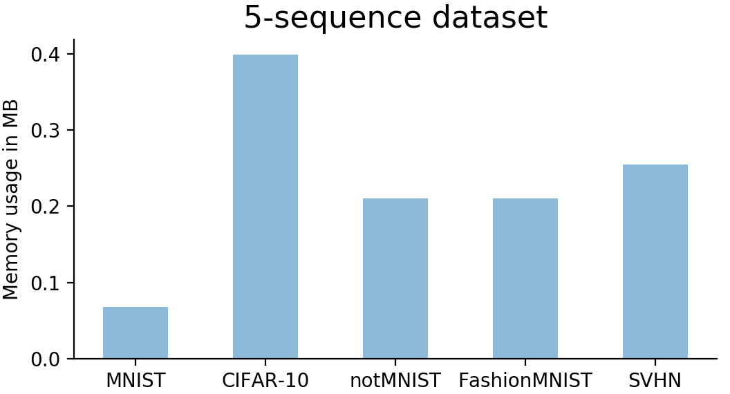
Figure 2: Dynamic memory allocation on 5-sequence dataset

[1.2] Method ACC% BWT% Size(MB) UCB [10] $76.34(0.12)$ $-1.34(0.04)$ $32.8$ ACL [11] 78.55(0.29) -0.00(0.15) 16.5 Baseline_UB 93.05(0.23) 0.00(0.00) 8.02 CACL ($\lambda_{sparse}=0.1$) 90.84(0.13) 0.00(0.00) 1.35

Figure 3: Comparison of CACL andstate-of-the-art approaches on 5-sequence dataset

5 Conclusion

In this work, we have proposed a compression based continual learning method that can dynamically grow a network to accommodate new tasks and uses low-rank approximations to achieve compact task representations. By encouraging the model to learn low-rank weight filters, we minimize the performance degradation during the compression phase and eliminate the time-consuming retraining step. By incorporating network factorization and a novel shared representational space, our method demonstrates state-of-the-art results on three datasets with highly compressed models. Our method manifests scalability to other architectures and also exhibits dynamic resource allocation based on the task. In this work, we assumed clear task boundaries exist between tasks and maintain individual task-identifiers during continual learning. In future work, we wish to eliminate such identifiers and further extend the compression/factorization strategy to linear layers.

Supplementary Material

Appendix A Architectural Details

A.1 5-layer CNN

Architectural details : We employ a simple 5 layer convolutional neural with convolutional layers of shape $64(3\times 3)-64(3\times 3)-128(3\times 3)-128(3\times 3)-256(2\times 2)$, where each convolutional block is of shape $channel(kernel\_height\times kernel\_width)$. We introduce intermediate dropout layers to regularize training. For each incoming task $t$ we attach $T^{t}_{head}$, where $T^{t}_{head}$ consist of a single linear layer that converts the convolutional features to task output.

Training details: We used $Adam$ optimizer for all the experiments with base learning rate $1e^{-3}$. We train each task for 200 epochs and drop the learning rate by factor of 10 at 80, 120, 180 epochs. We set $\lambda_{orth}=1.00$ to ensure equal importance to orthogonality regularizer($L_{orth}$) as task specific loss($L_{task}$). We set the pruning intensity parameter e to $1e^{-5}$.

A.2 VGG16_BN

Architectural details : We use the feature-extractor of VGG16_BN ignoring the final linear layers fc6, fc7, fc8 of VGG16 [23]. We use two linear layers for each task t as task-head $T^{t}_{head}$ to maintain similar number of task-specific parameters as in [15]. The four batch normalization parameters namely mean, variance, running_mean, running_variance for each batch-norm layer are stored separately for each task $t$ similar to [15].

Training details: We followed the same training strategy as for the 5-layer CNN. However, we set the sparsity loss weight, $\lambda_{sparse}$, to be $0.01$.

Appendix B Algorithms

We provide the pseudo code for our compression-aware training(Section 3.5) and compression(Section 3.6) in Algorithm 2, Algorithm3 respectively.

function TrainTask( $D_{t}$,   $[\mathcal{U}^{\leq t-1},\mathcal{S}^{\leq t-1},\mathcal{V}^{\leq t-1}]$, [ $\mathcal{U}^{t},\mathcal{S}^{t},\mathcal{V}^{t}$ ]):

      

      for $epoch\leftarrow 1,2,...epochs$ do

             for $batch\leftarrow 1,2,...batches$ do

                   ($x_{batch},y_{batch}$) $\sim$ $D_{t}$

                  

                  $\mathcal{U}^{t},\mathcal{V}^{t}\leftarrow\mathcal{U}^{t}-\nabla_{\mathcal{U}^{t}}(L_{task}+\lambda_{orth}L_{orth}),\mathcal{V}^{t}-\nabla_{\mathcal{V}^{t}}(L_{task}+\lambda_{orth}L_{orth})$

                  

                  $\mathcal{S}^{t}\leftarrow\mathcal{S}^{t}+\nabla_{\mathcal{S}^{t}}(L_{task}+\lambda_{sparse}L_{sparse})$

             end for

            

       end for

      return $\mathcal{U}^{t},\mathcal{S}^{t},\mathcal{V}^{t}$

      

Algorithm 2 Compression-aware training on task t

function Compression( [$\mathcal{U}^{t},\mathcal{S}^{t},\mathcal{V}^{t}$], $e$):

      

      for $l\leftarrow 1,2,...layers$ do

            

            $U,V,S=U^{t}_{l},V^{t}_{l},S^{t}_{l}$

              $\triangleright$ $U\in R^{c\times r},V\in R^{nhw\times r}$

            

            $ind=argsort(\{\sigma^{t}_{i\;l}\}^{r}_{i=1},desc)$

              $\triangleright$ Singular value indices descending order

             $U_{sort},V_{sort},S_{sort}=\;U[ind],V[ind],S[ind]$

              $\triangleright$ Sort the vectors

            

            $topk,energy_{curr}=\;0,0$

            

            $energy_{tot}=\sum_{i=1}^{r}(\sigma_{i\;l}^{t})^{2}$

              $\triangleright$ Total singular energy

            

            

            while $\frac{energy_{curr}}{energy_{tot}}<1-e$ do

                  

                   $energy_{curr}$ += $(\sigma^{t}_{topk\;l})^{2}$

                   topk = topk + 1

             end while

            

            $U^{t}_{pruned\>l},V^{t}_{pruned\>l},S^{t}_{pruned\>l}\leftarrow U_{sort}[:topk],V_{sort}[:topk],S_{sort}[:topk]$

            

            

              $\triangleright$ $U^{t}_{pruned\>l}\in R^{c\times topk},V^{t}_{pruned\>l}\in R^{nhw\times topk}$

            

       end for

      return $\mathcal{U}^{t}_{pruned},\mathcal{S}^{t}_{pruned},\mathcal{V}^{t}_{pruned}$

Algorithm 3 Compression for task $t$

Appendix C Additional Experiments

We present case-study results using CIFAR100 dataset(results using miniImageNet are discussed in Section 4.2 in the main paper) in Table 3. We find that CACL-ST effectively performs model compaction with minimal accuracy degradation. However, we find that CACL with shared representations consumes more memory than CACL-ST. This suggests selective sharing of representations might better help and we wish to explore this in our future work. Finally, we find that CACL-Fixed with limited memory constraint performs competitively when compared to others.

Method	ACC%	Size(MB)
Baseline_UB	$89.2(0.32)$	$31.67$
CACL-ST	88.9(0.12)	7.57
CACL-Fixed	82.15(1.07)	1.96
CACL	86.19(0.38)	8.68

Table 3: Case Study on CIFAR100

References

- Abdi and Williams [2010] H. Abdi and L. J. Williams. Principal component analysis. WIREs Comput. Stat., 2(4):433–459, July 2010. ISSN 1939-5108. doi: 10.1002/wics.101. URL https://doi.org/10.1002/wics.101.
- Saha et al. [2020] G. Saha, I. Garg, A. Ankit, and K. Roy. Structured compression and sharing of representational space for continual learning, 2020.
- Aljundi et al. [2018] R. Aljundi, F. Babiloni, M. Elhoseiny, M. Rohrbach, and T. Tuytelaars. Memory aware synapses: Learning what (not) to forget. In The European Conference on Computer Vision (ECCV), September 2018.
- Alvarez and Salzmann [2017] J. M. Alvarez and M. Salzmann. Compression-aware training of deep networks. In Proceedings of the 31st International Conference on Neural Information Processing Systems, NIPS’17, page 856–867, Red Hook, NY, USA, 2017. Curran Associates Inc. ISBN 9781510860964.
- Chaudhry et al. [2018] A. Chaudhry, P. K. Dokania, T. Ajanthan, and P. H. S. Torr. Riemannian walk for incremental learning: Understanding forgetting and intransigence. In V. Ferrari, M. Hebert, C. Sminchisescu, and Y. Weiss, editors, Computer Vision – ECCV 2018, pages 556–572, Cham, 2018. Springer International Publishing.
- Chaudhry et al. [2019a] A. Chaudhry, M. Ranzato, M. Rohrbach, and M. Elhoseiny. Efficient lifelong learning with a-gem. ArXiv, abs/1812.00420, 2019a.
- Chaudhry et al. [2019b] A. Chaudhry, M. Ranzato, M. Rohrbach, and M. Elhoseiny. Efficient lifelong learning with a-GEM. In International Conference on Learning Representations, 2019b. URL https://openreview.net/forum?id=Hkf2_sC5FX.
- Chaudhry et al. [2019c] A. Chaudhry, M. Rohrbach, M. Elhoseiny, T. Ajanthan, P. K. Dokania, P. H. S. Torr, and M. Ranzato. Continual learning with tiny episodic memories. ArXiv, abs/1902.10486, 2019c.
- Denton et al. [2014] E. L. Denton, W. Zaremba, J. Bruna, Y. LeCun, and R. Fergus. Exploiting linear structure within convolutional networks for efficient evaluation. In NIPS, 2014.
- Ebrahimi et al. [2019] S. Ebrahimi, M. Elhoseiny, T. Darrell, and M. Rohrbach. Uncertainty-guided continual learning with bayesian neural networks, 06 2019.
- Ebrahimi et al. [2020] S. Ebrahimi, F. Meier, R. Calandra, T. Darrell, and M. Rohrbach. Adversarial continual learning, 2020.
- French [1999] R. French. Catastrophic forgetting in connectionist networks. Trends in cognitive sciences, 3:128–135, 05 1999. doi: 10.1016/S1364-6613(99)01294-2.
- He et al. [2016] K. He, X. Zhang, S. Ren, and J. Sun. Deep residual learning for image recognition. In 2016 IEEE Conference on Computer Vision and Pattern Recognition (CVPR), pages 770–778, 2016.
- Hsu et al. [2018] Y.-C. Hsu, Y.-C. Liu, A. Ramasamy, and Z. Kira. Re-evaluating continual learning scenarios: A categorization and case for strong baselines. In NeurIPS Continual learning Workshop, 2018. URL https://arxiv.org/abs/1810.12488.
- Hung et al. [2019a] C.-Y. Hung, C.-H. Tu, C.-E. Wu, C.-H. Chen, Y.-M. Chan, and C.-S. Chen. Compacting, picking and growing for unforgetting continual learning. In Advances in Neural Information Processing Systems, pages 13647–13657, 2019a.
- Hung et al. [2019b] S. C. Y. Hung, J.-H. Lee, T. S. T. Wan, C.-H. Chen, Y.-M. Chan, and C.-S. Chen. Increasingly packing multiple facial-informatics modules in a unified deep-learning model via lifelong learning. In Proceedings of the 2019 on International Conference on Multimedia Retrieval, ICMR ’19, page 339–343, New York, NY, USA, 2019b. Association for Computing Machinery. ISBN 9781450367653. doi: 10.1145/3323873.3325053. URL https://doi.org/10.1145/3323873.3325053.
- Ioffe and Szegedy [2015] S. Ioffe and C. Szegedy. Batch normalization: Accelerating deep network training by reducing internal covariate shift. CoRR, abs/1502.03167, 2015. URL http://arxiv.org/abs/1502.03167.
- Jaderberg et al. [2014] M. Jaderberg, A. Vedaldi, and A. Zisserman. Speeding up convolutional neural networks with low rank expansions. ArXiv, abs/1405.3866, 2014.
- Kemker and Kanan [2018] R. Kemker and C. Kanan. Fearnet: Brain-inspired model for incremental learning. In International Conference on Learning Representations, 2018. URL https://openreview.net/forum?id=SJ1Xmf-Rb.
- Kirkpatrick et al. [2017] J. N. Kirkpatrick, R. Pascanu, N. C. Rabinowitz, J. Veness, G. Desjardins, A. A. Rusu, K. Milan, J. Quan, T. Ramalho, A. Grabska-Barwinska, D. Hassabis, C. Clopath, D. Kumaran, and R. Hadsell. Overcoming catastrophic forgetting in neural networks. Proceedings of the National Academy of Sciences of the United States of America, 114 13:3521–3526, 2017.
- Krizhevsky [2012] A. Krizhevsky. Learning multiple layers of features from tiny images. University of Toronto, 05 2012.
- Krizhevsky et al. [2012] A. Krizhevsky, I. Sutskever, and G. E. Hinton. Imagenet classification with deep convolutional neural networks. In Proceedings of the 25th International Conference on Neural Information Processing Systems - Volume 1, NIPS’12, page 1097–1105, Red Hook, NY, USA, 2012. Curran Associates Inc.
- Liu and Deng [2015] S. Liu and W. Deng. Very deep convolutional neural network based image classification using small training sample size. In 2015 3rd IAPR Asian Conference on Pattern Recognition (ACPR), pages 730–734, 2015.
- Lopez-Paz and Ranzato [2017] D. Lopez-Paz and M. Ranzato. Gradient episodic memory for continual learning. In Proceedings of the 31st International Conference on Neural Information Processing Systems, NIPS’17, page 6470–6479, Red Hook, NY, USA, 2017. Curran Associates Inc. ISBN 9781510860964.
- Mallya and Lazebnik [2018] A. Mallya and S. Lazebnik. Packnet: Adding multiple tasks to a single network by iterative pruning. 2018 IEEE/CVF Conference on Computer Vision and Pattern Recognition, pages 7765–7773, 2018.
- Mallya et al. [2018] A. Mallya, D. Davis, and S. Lazebnik. Piggyback: Adapting a single network to multiple tasks by learning to mask weights. In V. Ferrari, M. Hebert, C. Sminchisescu, and Y. Weiss, editors, Computer Vision – ECCV 2018, pages 72–88, Cham, 2018. Springer International Publishing.
- Riemer et al. [2018] M. Riemer, I. Cases, R. Ajemian, M. Liu, I. Rish, Y. Tu, and G. Tesauro. Learning to learn without forgetting by maximizing transfer and minimizing interference. CoRR, abs/1810.11910, 2018. URL http://arxiv.org/abs/1810.11910.
- Rolnick et al. [2018] D. Rolnick, A. Ahuja, J. Schwarz, T. P. Lillicrap, and G. Wayne. Experience replay for continual learning. In NeurIPS, 2018.
- Rolnick et al. [2019] D. Rolnick, A. Ahuja, J. Schwarz, T. Lillicrap, and G. Wayne. Experience replay for continual learning. In H. Wallach, H. Larochelle, A. Beygelzimer, E. Fox, and R. Garnett, editors, Advances in Neural Information Processing Systems 32, pages 350–360. Curran Associates, Inc., 2019. URL http://papers.nips.cc/paper/8327-experience-replay-for-continual-learning.pdf.
- Rusu et al. [2016] A. A. Rusu, N. C. Rabinowitz, G. Desjardins, H. Soyer, J. Kirkpatrick, K. Kavukcuoglu, R. Pascanu, and R. Hadsell. Progressive neural networks. ArXiv, abs/1606.04671, 2016.
- Serrà et al. [2018] J. Serrà, D. Suris, M. Miron, and A. Karatzoglou. Overcoming catastrophic forgetting with hard attention to the task. In ICML, 2018.
- Shin et al. [2017] H. Shin, J. K. Lee, J. Kim, and J. Kim. Continual learning with deep generative replay. In I. Guyon, U. V. Luxburg, S. Bengio, H. Wallach, R. Fergus, S. Vishwanathan, and R. Garnett, editors, Advances in Neural Information Processing Systems 30, pages 2990–2999. Curran Associates, Inc., 2017. URL http://papers.nips.cc/paper/6892-continual-learning-with-deep-generative-replay.pdf.
- Vinyals et al. [2016] O. Vinyals, C. Blundell, T. Lillicrap, K. Kavukcuoglu, and D. Wierstra. Matching networks for one shot learning. In Proceedings of the 30th International Conference on Neural Information Processing Systems, NIPS’16, page 3637–3645, Red Hook, NY, USA, 2016. Curran Associates Inc. ISBN 9781510838819.
- Xu et al. [2018] Y. Xu, Y. Li, S. Zhang, W. Wen, B. Wang, Y. Qi, Y. Chen, W. Lin, and H. Xiong. Trained rank pruning for efficient deep neural networks. ArXiv, abs/1812.02402, 2018.
- Yang et al. [2020] H. Yang, M. Tang, W. Wen, F. Yan, D. Hu, A. Li, H. Li, and Y. Chen. Learning low-rank deep neural networks via singular vector orthogonality regularization and singular value sparsification, 2020.
- Yoon et al. [2018] J. Yoon, E. Yang, J. Lee, and S. J. Hwang. Lifelong learning with dynamically expandable networks. ICLR, 2018.
- Zenke et al. [2017] F. Zenke, B. Poole, and S. Ganguli. Continual learning through synaptic intelligence. In Proceedings of the 34th International Conference on Machine Learning - Volume 70, ICML’17, page 3987–3995. JMLR.org, 2017.
- Zhang and Yang [2017] Y. Zhang and Q. Yang. A survey on multi-task learning, 2017.