Augmenting machine learning photometric redshifts with Gaussian mixture models

Abstract

Wide-area imaging surveys are one of the key ways of advancing our understanding of cosmology, galaxy formation physics, and the large-scale structure of the Universe in the coming years. These surveys typically require calculating redshifts for huge numbers (hundreds of millions to billions) of galaxies - almost all of which must be derived from photometry rather than spectroscopy. In this paper we investigate how using statistical models to understand the populations that make up the colour-magnitude distribution of galaxies can be combined with machine learning photometric redshift codes to improve redshift estimates. In particular we combine the use of Gaussian Mixture Models with the high performing machine learning photo-z algorithm GPz and show that modelling and accounting for the different colour-magnitude distributions of training and test data separately can give improved redshift estimates, reduce the bias on estimates by up to a half, and speed up the run-time of the algorithm. These methods are illustrated using data from deep optical and near infrared data in two separate deep fields, where training and test data of different colour-magnitude distributions are constructed from the galaxies with known spectroscopic redshifts, derived from several heterogeneous surveys.

1 Introduction

Many of the current key open questions in cosmology and extragalactic astronomy require extremely wide (probing large areas of the sky/volumes of the Universe) and deep (probing to extremely faint and/or distant sources) galaxy surveys to answer e.g. observations with Euclid (Laureijs et al., 2011) and the Vera C. Rubin Observatory (Rubin, formerly the Large Synoptic Survey Telescope, LSST, LSST Science Collaboration, 2009). To probe the time evolution/third dimension of the Universe, estimates of the redshift of each galaxy are typically required.

Galaxy (and Active Galactic Nuclei, AGN) redshifts can be calculated from their spectrum in two main ways, from spectroscopy or from photometry. Spectroscopic redshifts (‘spec-z’s’) are calculated by measuring the wavelength of a known spectral (normally emission) line or feature, and comparing it to the known rest frame wavelength of the line or feature. Photometric redshifts (‘photo-z’s’) are calculated by measuring the brightness of the galaxy in $N$ broad wavelength ranges, and mapping these brightnesses onto a redshift. Typically spec-z’s are far more precise than photo-z’s, but can only be measured for much smaller populations of galaxies as spectroscopic observations are more costly, and generally reach shallower depths, see Fernandez‐Soto et al. (2001) for a comparison of the strengths and weaknesses of both classes of measurement.

Photometric redshifts themselves can be calculated in two main ways; ‘template fitting’ methods and ‘machine learning’ methods. Template fitting methods are essentially ‘theory’ based methods - we attempt to use our understanding of the physics behind galaxy spectral energy distributions to map photometry to a spectrum. This in practice can take a number of forms, but typically consists of using a number of model template spectra (either using synthetic spectra or spectra extracted at low-redshift from galaxies with observations at many wavelengths), and using a $\chi^{2}$-minimisation-like method to find the ‘best’ redshift. Notable template-fitting based codes include Photometric Analysis for Redshift Estimate (LePhare, Arnouts et al., 1999; Ilbert et al., 2006), Bayesian Photometric Redshifts (BPZ, Benitez & Narciso, 1998; Benitez et al., 2004; Coe et al., 2006), the Zurich Extragalactic Bayesian Redshift Analyzer (ZEBRA, Feldmann et al., 2006), EAzY (Brammer et al., 2008) and Phosphoros (Paltani et al. in prep). Machine learning photo-z methods are typically entirely data based; a machine learning algorithm is given a set of galaxies with photometry and known (usually spectroscopic) redshifts, and is then tasked with predicting the redshift of galaxies without known spec-z’s. Widely used machine learning photo-z codes include Artificial Neural Network Redshifts (ANNz2, Collister & Lahav, 2004; Sadeh et al., 2016), Trees for Photo-Z (TPZ, Carrasco Kind & Brunner, 2013), Self Organizing Map Redshifts (SOMz, Carrasco Kind & Brunner, 2013), Machine-learning Estimation Tool for Accurate PHOtometric Redshifts (METAPHOR, Cavuoti et al., 2017), FRANKEN-Z (Speagle et al., in prep.) and many more. The resulting photometric redshifts are required for a variety of science goals (see Desprez et al., 2020, for a recent photo-z code comparison in the context of Euclid objectives, and Schmidt et al., 2020 in the context of Rubin), but one of the most important, with the most stringent requirements, is weak lensing, where the matter power spectrum is measured by the shear on galaxy shapes, but accurate unbiased redshift estimates are needed for unbiased cosmological inferences, e.g. Banerji et al. (2008); Abdalla et al. (2011); Hearin et al. (2010); Hildebrandt et al. (2017); Hoyle et al. (2018). Finally Salvato et al. (2019) present a comprehensive review of contemporary photometric redshift methods, applications and challenges, and a discussion of what advanced approaches must be developed for surveys to best meet their scientific goals in the future.

In this work we consider how using Gaussian Mixture Models (GMMs), a Bayesian approach to dividing a set of objects into sub-populations can support the machine learning photo-z code GPz (Almosallam et al., 2016b, a) - although the approach could be employed with other algorithms. In particular we investigate using GMMs to a) help account for the different colour space distributions of the training and test data and b) exploit the fact that galaxies and AGN naturally fall into different populations. The approach has some similarities to that described in Fotopoulou & Paltani (2018), who divide their galaxies into separate galaxy populations as part of the photometric redshift calculation process (but for a template fitting method), and also Lima et al. (2008), who use weighting schemes to estimate the redshift distribution, accounting for differences in colour distributions to a reference sample.

The structure of this paper is as follows. In Section 2 we describe the algorithms used in this study, namely GPz and a GMM algorithm, and the data used. In Section 3 we discuss the methods developed. In Section 4 we present our results, discuss the consequences in Section 5, concluding in Section 6.

2 Preliminaries

2.1 GPz

GPz is a machine learning regression algorithm originally developed for the problem of calculating photometric redshifts; the details of the algorithm and the key developments in machine learning (ML) theory are described in Almosallam et al. (2016b, a). The algorithm is ‘sparse Gaussian process’ (GP) based, e.g. see Rasmussen & Williams (2006). A Gaussian process is a stochastic process with a random variable defined at each point in a space of interest, such that any linear combinations of random variables from different points has a Gaussian distribution; essentially an un-parametrised continuous function defined everywhere with Gaussian uncertainties. GPs are very flexible class of supervised non-linear regression algorithm that make very few explicit parametric assumptions about the nature of the function. For this reason they are well-suited for modelling complex non-linear mappings like photometric redshifts (Rasmussen & Williams, 2006; Bonfield et al., 2010; Almosallam et al., 2016b). A GP based ML algorithm will typically take some set of data over the parameter space of interest and in some sense try and find the Gaussian process that was most likely to have produced the data - and then make predictions for other parts of parameter space based on that. The key features introduced by GPz include a) implementation of a sparse GP framework, allowing the algorithm to run in $O(nm^{2})$ instead of $O(n^{3})$ (where $n$ is the number of samples in the data and $m$ is the number of basis functions), b) a ‘cost sensitive learning’ framework where the algorithm can be tailored for the precise science goal, and c) properly accounting for uncertainty contributions from both variance in the data as well as uncertainty from lack of data in a given part of parameter space (by marginalising over all the GPs that could have produced the data). GPz was further tested and developed in Gomes et al. (2018) who measured the improvement that could be achieved by also including near-infrared bands and angular sizes, as well as introducing a post-processing calibration that reduced the bias (the difference between the true/spectroscopic redshift, and the photo-z estimate, $z_{\textrm{spec}}-z_{\textrm{phot}}$). Duncan et al. (2018) introduced combining GPz with template-based photometric redshifts using a hierarchical Bayesian model that gave better photometric redshifts than ML or template fitting alone could have produced (a hybrid approach was also considered in Desprez et al., 2020). GPz is also beginning to be used in other astronomy and physics applications e.g. building surrogate models for and quantifying the uncertainty on inertial confinement fusion experiments (Hatfield et al., 2020) and orbital dynamics (Peng & Bai, 2019).

Two key deficiencies of GPz as applied to photo-z’s are a) GPs ordinarily only produce Gaussian uncertainties, whereas the true probability distribution of a galaxy’s redshift based on its photometry is typically not Gaussian, and b) typically the target galaxy population has a different colour distribution than the colour distribution of the training set, which introduces biases (a problem common to all machine learning based approaches). In this paper we attempt to account for and mitigate against these difficulties.

Unless otherwise stated, we use the settings in Table 1 (see Almosallam et al., 2016b, a for precise definitions and interpretations).

Table 1: Parameter setting of GPz.

Parameter	Value	Description
$m$	500	Number of basis functions; complexity of GP, in general higher $m$ is more accurate but longer run time
maxIter	500	Maximum number of iterations
maxAttempts	50	Maximum iterations to attempt if there is no progress on the validation set
method	GPVC	Bespoke covariances on each basis function
normalize	True	Pre-process the input by subtracting the means and dividing by the standard deviations
joint	True	Jointly learn a prior linear mean-function

2.2 GMMs

Mixture Models are probabilistic models for modelling data with sub-populations, where the observed data does not identify which population a datum is from. An everyday example of a Mixture Model could be length of publication measured in number of words; the distribution would have separate populations of letters, journal articles and books with very different word length, but typically it would not be possible to separate out short articles from long letters etc. Common astronomical examples include identifying star clusters, identifying populations in surveys, deciding how many classes of a source exist etc. see Kuhn & Feigelson (2017), and they have also been used for more complex tasks like the identification of strong gravitational lenses (e.g. Cheng et al., 2020). Gaussian Mixture Models (GMMs) are a specific type of mixture where each mixture has a Gaussian distribution. GMMs can be viewed as an example of unsupervised machine learning, in that the algorithm is not told in advance what or how many populations there should be or given any examples of members of populations. See also D’Isanto & Polsterer (2018) who use a mixture density network to make a GMM of the galaxy redshift posterior.

More formally, we would like to maximize the likelihood distribution:

$$p(\mathbf{X})=\Pi_{i=1}^{n}p(\mathbf{x}_{i}),$$ (1)

where $\mathbf{X}=\{\mathbf{x}_{i}\}_{i}^{n}$ is the set of samples in the data set, $\mathbf{x}_{i}\in\mathbb{R}^{d}$ is the $i$-th sample in the data set, $d$ is the dimensionality of the input and $p(\mathbf{x})$ is some multivariate probability density function. Assuming a multivariate normal Gaussian distribution for $p(\mathbf{x})$, the parameters of the distribution that would maximize the likelihood of observing the data, the mean and covariance, can be computed analytically. However, as discussed previously most distributions found in the real world are more complex than a simple unimodal normal distribution. We can model a more complex distribution by assuming that $p(\mathbf{x})$ is the marginal distribution over some latent variable $j$ as follows:

$$p(\mathbf{x}_{i})=\sum_{j=1}^{k}p(\mathbf{x}_{i}|j)p(j).$$ (2)

In effect we have modelled the probability density function $p(\mathbf{x})$ as a weightinged sum of Gaussian distributions, i.e. a Gaussian Mixture Model. An important property of GMMs, is that they can, for some number of mixtures $k$, model any non-standard probability distribution. The goal now is to find the $k$ means, covariances and mixture weightings that would maximize the probability of observing the data. This typically cannot be solved analytically, and normally requires optimization techniques. The Expectation Maximization (EM) algorithm is an iterative method that can be used to search for such parameters. However, the EM algorithm is prone to over-fitting especially as the number of mixtures is increased (at the limit when $k=n$, the means will correspond to the data locations and covariances will be close to zero). To overcome this, we use a Variational Bayes (VB, see Jordan et al., 1999; Jaakkola & Jordan, 2000) approach that puts priors on the means, covariances and mixture weightings to always find the optimal set of mixtures; even if $k$ is set too high it will automatically prune the extra mixtures by setting their mixture weightings to zeros.

2.3 Data

In a realistic scenario, all galaxies with spectroscopic redshifts would be the training set, and all sources without would be the target test set. Coping with the training and test data sets having different colour-magnitude distributions is a major challenge for ML based photo-z calculations e.g. see Beck et al. (2017). Unfortunately however, the nature of the problem is that it is difficult/impossible to measure the performance on the galaxies without spec-zs. To overcome this problem, and test how our method performs when the test and training data have different distributions, we construct training and test data sets for which both have spectroscopic redshifts.

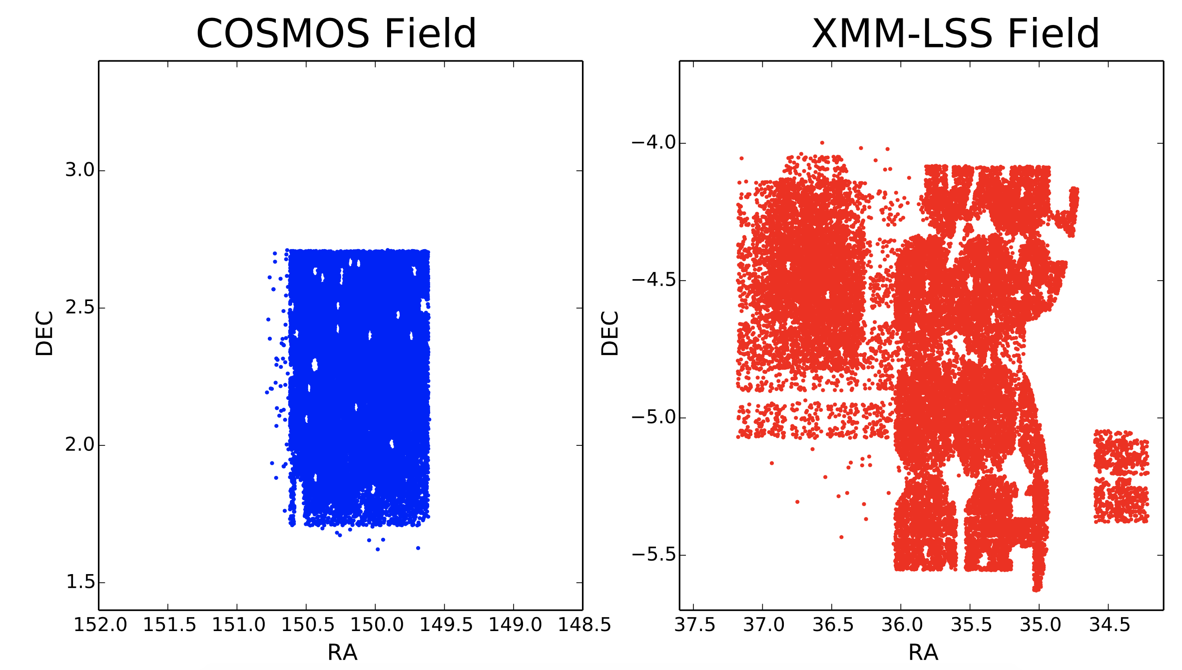
Figure 1: Field geometry of galaxies used in this analysis (each of which has a spectroscopic redshift). The ‘COSMOS’ galaxies are used for training, and the ‘XMM-LSS’ galaxies for testing. The unusual field geometries result from the complex ways in which the various photometric and spectroscopic surveys have overlapped and intersected.

In order to ensure a rigorous test of the methods we consider two separate deep field data sets, but which have similar photometric coverage. Our training data is from the COSMOS field, and the test data from the XMM-Newton Large-Scale Structure (XMM-LSS) field - see figure 1. We use the catalogues constructed in Bowler et al. (2020) and Adams et al. (2020), which, in order to ensure consistency, used identical procedures to extract the photometry across the two fields. Sources were selected in the K_s band, and forced photometry was performed on all the other bands. We use 2” diameter circular apertures, which had an aperture correction applied by a model generated with PSFEx (Bertin, 2011) for each band.

For this paper we use the photometry in 10 filters; $u$ (CLAUDS, CFHT, for both COSMOS and XMM-LSS, Sawicki et al., 2019), GRIZY (HSC-SSP, for both COSMOS and XMM-LSS, Aihara et al., 2017) and YJHK_s (VIDEO-VISTA for XMM-LSS, Jarvis et al., 2013 and UltraVISTA for COSMOS, McCracken et al., 2012; Laigle et al., 2016), but to a range of different depths, meaning both the colour space probed and the uncertainty on the photometry are quite inhomogeneous - even though the photometry extraction was done in a very homogeneous manner. The end result is two catalogues that span colour-magnitude space very differently, but with photometry very consistent for comparisons between individual galaxies in the two fields.

Similarly the spectroscopic redshifts come from a range of sources, curated in the same way as in Adams et al. (2020). The spec-zs are taken from the VVDS (Le Fèvre et al., 2013), VANDELS (McLure et al., 2018; Pentericci et al., 2018), Z-COSMOS (Lilly et al., 2009), SDSS-DR12 (Alam et al., 2015), 3D-HST (Skelton et al., 2014; Momcheva et al., 2016), Primus (Coil et al., 2011; Cool et al., 2013), DEIMOS-10K (Hasinger et al., 2018) and FMOS (Silverman et al., 2015) surveys. We would note that machine learning based photo-z methods are reliant on the accuracy of the spectroscopic redshifts in the training sample. If the spec-zs used in the training process are inaccurate then machine learning methods will simply reproduce the incorrect spec-z values. For this reason we only used the most secure spec-zs that have flags indicating high quality (confidence of $\geq$ 95 per cent). Where a source had a secure spec-z available from more than one survey, the mean of the secure redshifts was used. Furthermore, we found that the Primus spec-zs were often inconsistent with the higher-resolution spec-zs and template-based photo-zs at $z>1$. For this reason we only use the $z<1$ Primus spec-zs. The resulting combination of spectral and photometric data used here is thus similar to that presented in Adams et al. (2020) and Bowler et al. (2020).

The XMM-LSS data set constructed includes data from the VANDELS survey, with redshifts in the $z=1-4$ range, which are underrepresented in the COSMOS data for $z>2.5$. This means a) our training and test data have different colour distributions and b) our test data has a high-redshift tail not present in the training data. There are 29,663 galaxies in the COSMOS training set and 24,534 galaxies in the XMM-LSS testing set.

In terms of stellar contamination, as we have tried to ensure that we are only using ‘secure’ redshifts, the vast majority of our sources should be extragalactic. More generally for photo-zs, stars can typically be removed based on a morphological cut (e.g. remove point sources, which will also remove quasars) or with a colour-cut. Conversely, our sample likely has a moderate number of AGN - both in terms of sources that are dominated by AGN light, as well as Seyfert-like galaxies whose photometry has large contributions from both galaxy starlight and a central nucleus. X-ray data is available in both the COSMOS field (Marchesi et al., 2016) and the XMM-LSS field (Chen et al., 2018), and could in principle be used to identify AGN (considered for some of the sources in this sample in Adams et al., 2020). We chose however not to use the x-ray data to remove AGN in this work on the rationale that machine learning methods should in principle be agnostic with regards to whether the source is a galaxy or an AGN - as long as there are similar sources with secure redshifts in the training set it should be possible to give sources accurate machine learning based photo-zs. This conversely is not the case for template based methods; if templates with sufficient AGN contribution are not included in the fitting process then in general Seyfert-like galaxies can receive inaccurate redshifts (a point discussed in greater detail in Salvato et al., 2019). The converse strategy of separating a sample into AGN and non-AGN populations in advance is studied in Norris et al. (2019), who measure photo-z performance when x-ray detected sources are included or not included in their training data. We chose not to study AGN versus non-AGN performance separately in this work in order to focus on how to improve global performance, although making such divisions may be a useful method for some science goals.

The way the data sets are constructed from a range of photometric and spectroscopic sources means that they do not have single well defined depths, and in general have different colour and redshift distributions. For approximate reference however the 95th percentile faintest training (testing) sources have AB magnitudes $u=26.9$ ($=26.9$), $G=25.6$ ($=25.5$), $R=24.6$ ($=24.4$), $I=24.1$ ($=23.9$), $Z=23.8$ ($=23.6$), $Y_{\textrm{HSC}}=23.6$ ($=23.6$), $Y_{\textrm{VIDEO}}=23.6$ ($=23.6$), $J=23.3$ ($=23.5$), $H=23.2$ ($=23.4$) and $K_{\mathrm{s}}=23.1$ ($=23.3$). Note these are representative depths of spectroscopic data, not the imaging depths. No cosmology is need to be assumed in this work for any of the photometric or redshift calculations.

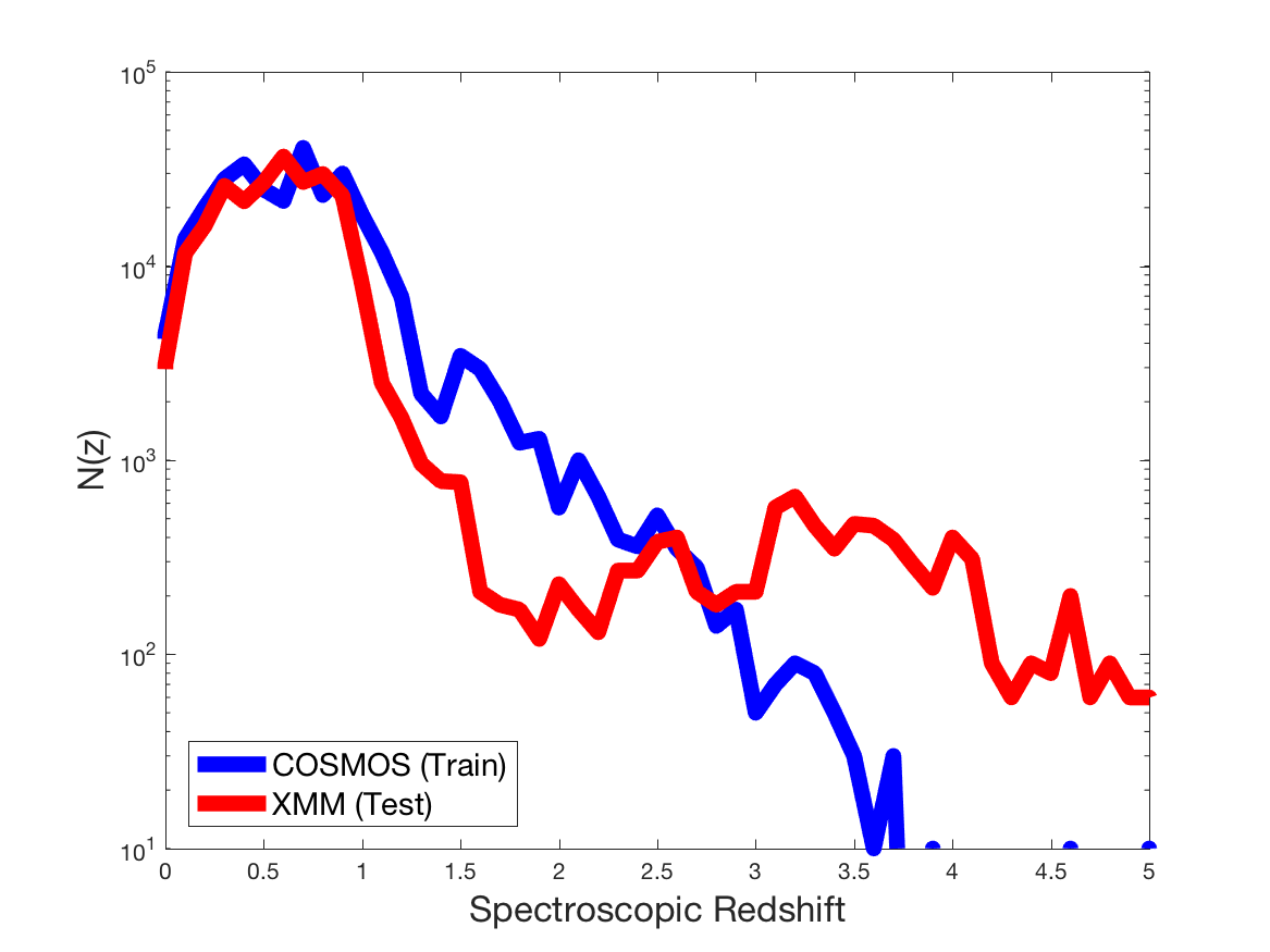
Figure 2: The spectroscopic redshift distributions of the galaxies in the two samples used in this study, the ‘COSMOS’/training data, and the ‘XMM-LSS’/testing data.

3 Methods

3.1 Generalised Cost-Sensitive-Learning

A key property of GPz is the ability to tailor the weighting for different science applications. Almosallam et al. (2016b) presented three different weightings, ‘Normal’, ‘Normalised’, and ‘Balanced’. Normal weighting weightings each galaxy the same (the ‘null’ option), Normalised weightings each galaxy in the training set by $1/(1+z_{\mathrm{spec}})$, and Balanced weightings each galaxy inversely proportional to the number of galaxies with that redshift in the training set (e.g. galaxies with under-represented redshifts are upweightinged).

Here we add to this Generalised Cost-Sensitive-Learning (GCSL) weighting. We model the training set colour-magnitude space with a GMM to find $p_{\mathrm{train}}(\textbf{x})$, and do the same for the colour-magnitude space of the test set of data to find $p_{\mathrm{test}}(\textbf{x})$(where x is the colour-magnitude photometry space of the data). This is essentially using the GMM to model the probability distribution in an unbiased way. We then set the weighting for GPz as:

$$w_{i}=\frac{p_{\mathrm{test}}(\textbf{x}_{i})}{p_{\mathrm{train}}(\textbf{x}_{i})}.$$ (3)

This potentially improves over balanced weighting a) because it weightings galaxies in colour space rather than redshift space (different parts of colour space correspond to the same redshift) and b) it accounts for the colour-magnitude distribution of both the training set and the test set, rather than just the training set (it essentially generalises the approach used in Lima et al., 2008 and Duncan et al., 2018). A small number of extreme outlier galaxies end up with extremely high weightings which were found to distort the entire training process, so we a) cap the maximum weighting at 20, and b) instead of equation 3, we in practice use $w_{i}=\frac{p_{\mathrm{test}}(\textbf{x}_{i})+\epsilon}{p_{\mathrm{train}}(\textbf{x}_{i})+\epsilon}$ with $\epsilon=0.01$ to avoid extreme ratios at parts of parameter space with low data densities. Figure 3 shows (a 2D projection of) the different colour spaces of the training and test data sets, the mixtures that were identified, and the corresponding $w_{i}$ values. Figure 4 shows a histogram of resulting $w_{i}$ values.

If the test set and the training set have the same colour distribution GCSL reduces to ‘Normal’ weighting as $p_{\mathrm{train}}$ and $p_{\mathrm{test}}$ will be identical and the $w_{i}$ will be equal to one. In this scenario, for rare parts of colour-magnitude space, the performance will be low, but that is unimportant because a proportionately small number of galaxies in the test set will have that colour. Balanced is near-equivalent to when the test set has a uniform distribution in colour space, or equivalently desiring a homogeneous performance in colour space. ‘Normalised’ makes the science judgement that we value percentage error on $1+z$ rather than absolute error on $1+z$, as opposed to weighting on sample distributions. One could in principle weighting by ‘Normalised-GCSL’ with $w_{i}^{\mathrm{Normalised-GCSL}}=w_{i}^{\mathrm{GCSL}}/(1+z_{i})$, although we found in practice this made relatively little difference.

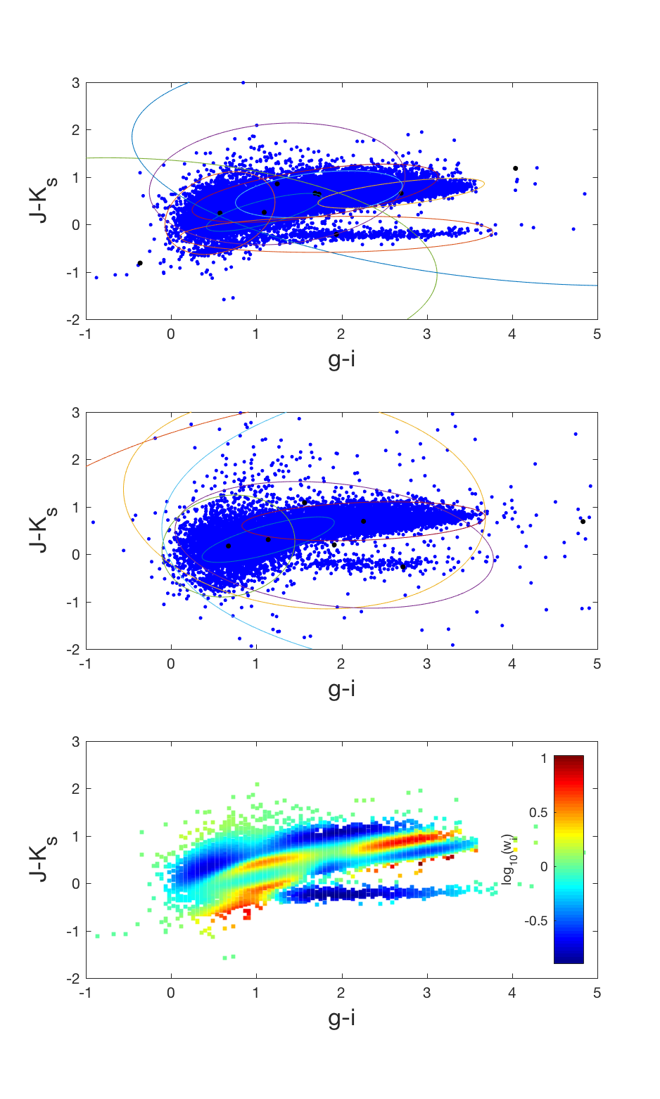
Figure 3: The (g-i)-(J-K_s) plane for the training (top sub-plot) and test (middle sub-plot) data. Ellipses show the identified mixtures (projected into 2D), with black marks showing the mixture centres. The lower plot shows the $w_{i}$ values for the training data (essentially the ratio of the data density of the top and middle plots). A stellar locus is visible (c.f. Figure 6a in Baldry et al., 2010).

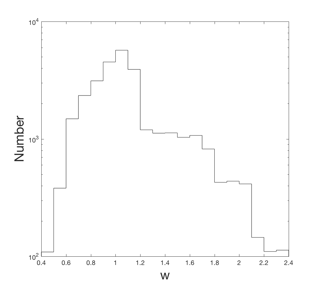
Figure 4: Distribution of $w_{i}$ values found (note that $w_{i}$ is capped at 20).

From figure 3 it can be seen that there is some stellar contamination in the sample (the population at $\mathrm{J}-\mathrm{K}_{\mathrm{s}}\approx-0.2$, see Figure 6a in Baldry et al., 2010), despite them nominally being spectroscopically confirmed galaxies (as is likely to be the case at least to some degree in any putative Euclid and Rubin data set). However it can be seen that the GMMs do identify the stars as being a separate component in colour-colour space (and down-weighting them, as there do not appear to be as many in the test spec-z sample), so future work could include a probability of each mixture to correspond to a stellar component.

3.2 Weighted Validation

Machine learning algorithms generally divide the labelled data into training and validation data sets when training the algorithm. The algorithm typically fits parameters to the training data, measures how well it does on the validation data, and then updates the complexity of the model (if over/under fitting) appropriately based on this. Since we are ultimately trying to predict the test data, making the validation data look more like the test data might help the model better tune itself. To do this, we take each galaxy with a spectroscopic redshift in the COSMOS data set and probabilistically select it to be either training or validation according to:

$$P_{\mathrm{train}}=\frac{1}{1+w_{i}}$$ (4)

and

$$P_{\mathrm{valid}}=\frac{w_{i}}{1+w_{i}},$$ (5)

where $P_{\mathrm{train}}$ is the probability of the galaxy being assigned to the training data set, $P_{\mathrm{valid}}$ is the probability of the galaxy being assigned to the validation data set and $w_{i}$ is the weighting from equation 3. Weighted Validation is similar in some regards to Generalised Cost-Sensitive-Learning but may potentially cope slightly better with parts of parameter space with low data density.

3.3 Resampling

As already mentioned, GP based ML methods, including GPz, by definition only give Gaussian uncertainties. This is typically not realistic for photometric redshifts. To generate non-Gaussian ML posteriors with GPz we trial a resampling method, where GPz is run a large number of times on slightly perturbed copies of the data to produce a large number of Gaussians, which are then summed to produce a non-Gaussian pdf. This is similar to the photometry perturbations of METAPHOR (Cavuoti et al., 2017), and the Monte Carlo approach of FRANKEN-Z (Speagle et al., in prep.).

The resampling method consists of the following steps:

1. For each galaxy in the training and test sets, based on the uncertainty on each magnitude, resample a new magnitude value for each band

2. Train GPz on this resampled set of training data

3. Produce Gaussian pdfs for the resampled test data

4. Repeat Steps 1-3 $s$ times

5. Average the $s$ pdfs produced to obtain the final pdf

This procedure lets us probe all the variation in the data. The hope is that for galaxies near ‘cliffs’, that are assigned one redshift with a very small uncertainty, but are very close in colour-magnitude space to galaxies that assigned very different redshifts also with small uncertainty, that the ‘cliff’ is repositioned slightly each time and the galaxies get more realistic pdfs. This approach can be thought of as a numerical method for GPz with noisy input. GPz conventionally accounts for noisy input, but still produces a single Gaussian. This approach approximates, at the limit of large ‘$s$’, a multi-modal Gaussian for a ‘noisy’ input of variance equal to the perturbation variance. Of the methods suggested in this text, this is by far the most computationally expensive, as it increases the runtime by a factor of $s$. However, because of the sparse framework used, GPz runs very fast and it remains practical to use $s\sim 100$ on a laptop (as used in this analysis), and would be viable to use a much higher $s$ on a cluster as each ‘run’ of GPz can be parallelised.

3.4 Exploiting the Population Structure

Galaxies naturally fall into different populations. We can use the GMM to find natural galaxy populations, and assign probabilities of being in each population. Given a GMM, and for each galaxy a discrete probability density function for being in each of the populations, there are two natural ways to couple this to a ML algorithm, which we discuss below.

In the basic application of GPz, training the algorithm is $O(nm^{2})$ in number of samples $n$ and in number of basis functions $m$ used to represent the mapping from photometry to redshift (in general a higher $m$ will give better results, but take longer to train). Here we propose using the GMM to split colour space into $k$ regions, and then running GPz with $m/k$ basis functions in each region (we call this ‘GMM-Divide’). This typically will reduce the run time by a factor of $\sim k$ - each region will run $\sim k^{2}$ times faster, but $k$ regions must be run. Regions are defined by which Mixture has the highest probability for that point in colour-magnitude space (a galaxy is in the region of the population it is most likely to be in). It is technically possible for the region for some Mixtures to be the empty set e.g. tiny Gaussian within a broader one with a much larger amplitude. Regions are thus completely algorithmically determined by the GMM, with no human intervention; see figure 3. We define regions of the colour-magnitude distribution of the test set, and separate both the training and test set based on that region division. There are many slight variations on exactly how the GMM algorithm can find populations; we found that letting it select in a magnitude and colour space (see figure 3) gave the best results although precise implementation does not appear to make a large difference. The approach of splitting up parameter space into multiple regions has some similarities to the method of Masters et al. (2015), who use Self-Organising Maps (SOMs) rather than Gaussian Mixture Models as the unsupervised learning model used to divide up colour-magnitude space. There is also some overlap to the approach of separating AGN and non-AGN in advance described in Norris et al. (2019); if x-ray data is available for the training process, then separating based on whether or not a source is x-ray detected is essentially dividing the sample into two populations based on a flux cut. The GMM here attempts to make such divisions in an unsupervised manner.

The other natural approach, which we investigated, would be to let galaxies be in multiple populations probabilistically e.g. for each population, we train GPz on the entire training set with weightings proportional to how likely they were to have been drawn from that population i.e. $w_{i}=P(\textrm{galaxy $i$ in population $h$})$. We then calculate a redshift pdf for each galaxy in the training set for each population. These are then summed in proportion to the probability that each galaxy in the test set was in each population (e.g. if there was a 75 percent probability the galaxy was drawn from population 1, and a 25 percent chance it was drawn from population 2, the Gaussians from GPz run for population 1 and population 2 are summed with a 3:1 weighting). However we found that the vast majority of galaxies were in a given population with probability near 1, and that this approach did not typically give better predictions.

3.5 Predicting $\mathrm{log}(z)$

With the exception of Andromeda and other bodies in the Local Group, all galaxies have a positive redshift. Machine learning based redshift predictions can sometimes have non-trivial fractions of the resulting pdf be negative. One way of coping with this is to effectively set a strong prior that redshift has to be non-negative (essentially cut off the negative part of the pdf). This unfortunately has the result of introducing a bias in the predictions for low redshift galaxies (because this approach means you can only over-estimate, never underestimate). We test the alternative of trying to predict $\mathrm{log}(z)$, which now takes all values, rather than $z$ (considered in Section 3.3 of Almosallam, 2017). Note that if $\Theta=\mathrm{log}(z)$, $\mathbbold{E}(z)\neq\exp(\mathbbold{E}(\Theta))$; Almosallam (2017) show $\mathbbold{E}(z)=\exp(\mathbbold{E}(\Theta)+\frac{1}{2}\mathbbold{V(\Theta)}))$ and $\mathbbold{V}(z)=(\exp(\mathbbold{V}(\Theta))-1)\times(\mathbbold{E}(z))^{2}$.

This problem is to some degree similar to the issue of treatment of negative fluxes; fluctuations in the noise can lead to galaxies being assigned negative fluxes through the data reduction process (although hopefully with uncertainties that make the measurements consistent with zero flux). When we train our photometric redshift model, we use log-fluxes i.e. implicitly assuming uncertainties on fluxes are Gaussian in log-space. For negative flux values we resample from a Gaussian centred on the negative value, with standard deviation the associated error, until a positive value is found. This obviously gives a slight bias for the faintest galaxies, however, for these sources the uncertainty on the flux is high and as the uncertainty is used within GPz it has negligible effect. An alternative way to deal with negative fluxes is to use luptitudes (Lupton et al., 1999), as used with GPz in Desprez et al., (2020). Fluxes typically have Gaussian uncertainty in linear-space near the detection threshold, but Gaussian uncertainty in log-space for brighter sources. The luptitude transformation essentially transforms the flux in such a way as to smoothly transition between these two regimes. Unfortunately however this requires consistency of detection threshold (which is used in the transformation), and the detection thresholds are not uniform between the different surveys we use to make up our two samples, so a luptitude in one would not necessarily correspond to the same luptitude in another. Both the method employed here and luptitudes are not completely accurate, however the effect on our results is minimal.

4 Results

In this section we trial the methods discussed in Section 3 on the data described in Section 2.3. We calculate photometric redshifts using the following methods:

• Base performance, ‘Normal’ weighting

• ‘Generalised CSL’ weighting (section 3.1)

• Weighted Validation (section 3.2)

• Resampled base performance as per section 3.3 with $s=100$

• GMM-Divide (section 3.4)

• Modelling $\mathrm{log}(z)$ (section 3.5)

• ‘All’ - Weighted Validation’, GMM-Divide and Resampling done simultaneously

Figure 5 shows spec-z versus photo-z for these methods, with varying performance. We also show for reference results if only the 70 percent of data with lowest predicted uncertainty from ‘All’ is used (‘Best’).

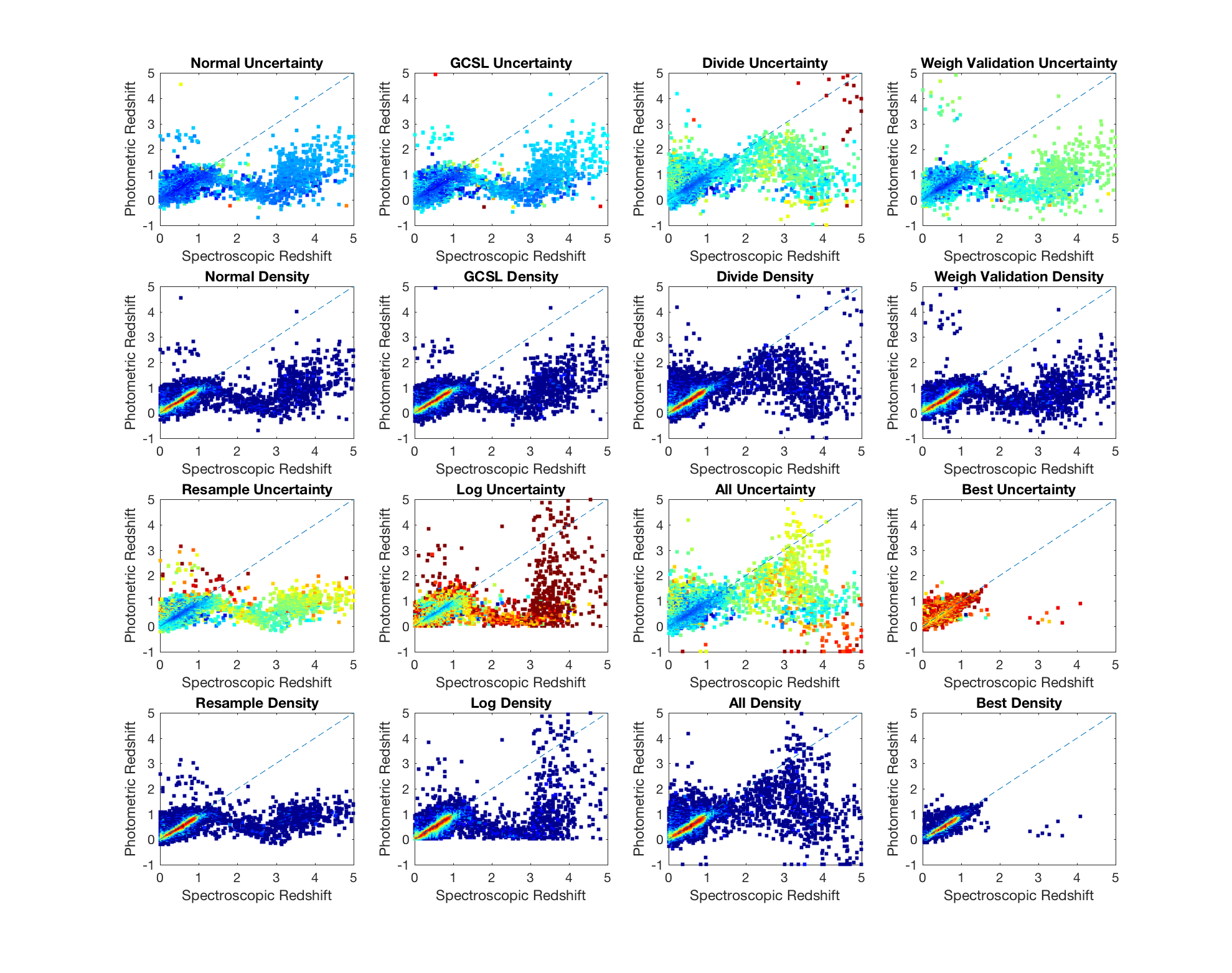
Figure 5: Spectroscopic redshift versus photometric redshift for the Normal implementation, Generalised-CSL, GMM-Divide and Weighing Validation methods (top two rows, going left to right) and the resampling, log, ‘All’ and ‘Best’ methods (bottom two rows, going left to right). The first and third rows are coloured by the predicted uncertainty, the second and fourth by the data density.

4.1 Metrics

Figures 6, 7, and 8 compare the performance of our methods as measured by the root mean squared error (RMSE), bias ($z_{\textrm{spec}}-z_{\textrm{phot}}$), and fraction of sources within 15 percent of the true value (FR15), see table 1 in Gomes et al. (2018). These quantities are expressed as a function of ‘fraction of the data’ (the data is divided into bins of ‘error bar size’, so ten percent corresponds to a bin of the best tenth of galaxies in terms of uncertainty size etc.). For RMSE, we also show the data as a function of spectroscopic redshift.

RMSE is approximately 0.05 for the data with the smallest uncertainties, and increases to about 0.25 for the data with the largest uncertainties. As a function of (spectroscopic) redshift we find the RMSE $\approx 0.2$ at $z\sim 0.75$, and $\approx 3$ at high redshift. As a function of $K_{\mathrm{s}}$-band magnitude the RMSE is between 0 and 0.5 for most magnitudes, but rises rapidly for $K_{\mathrm{s}}>23$ and $K_{\mathrm{s}}<17$ galaxies, where there is less training data. FR15 varies from essentially 100 percent for the data with the smallest uncertainties, to around 85 percent for the data with the largest uncertainties, dropping off sharply for the final 30 percent of the data, as one would expect. Bias is less than 0.02 for most of the data, apart from the 20 percent with the largest uncertainties. The different methods gave moderate variability; in particular ‘Resampling’ improved RMSE and FR15, but increased the bias. ‘Weighted validation’ was the only method to largely improve the bias.

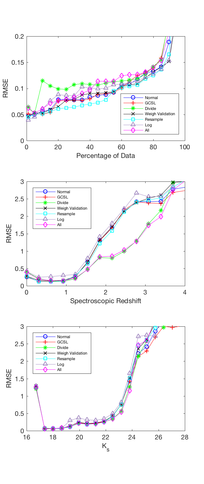
Figure 6: Root mean squared error on on the photometric redshifts, as a function of a) percentile of the data (top plot, zero with the smallest uncertainties, 100 the largest), b) spectroscopic redshift (centre plot) and c) $K_{\mathrm{s}}$ band magnitude (bottom plot).

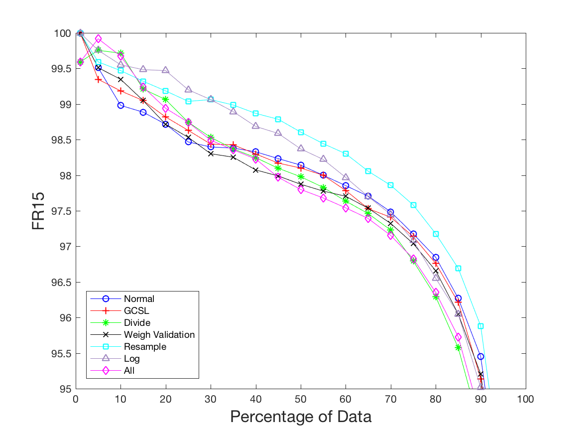
Figure 7: FR15 on on the photometric redshifts, as a function of percentile of the data (zero with the smallest uncertainties, 100 the largest).

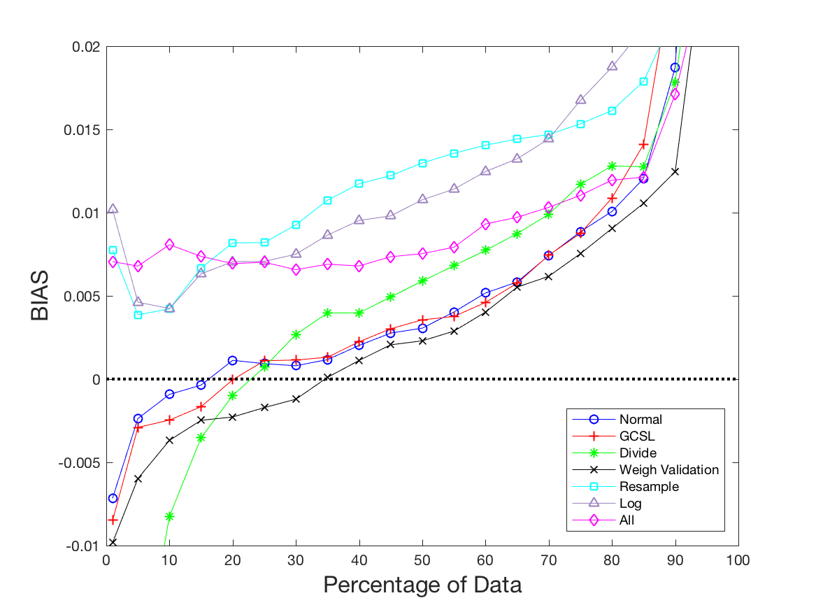
Figure 8: Bias on on the photometric redshifts, as a function of percentile of the data (zero with the smallest uncertainties, 100 the largest).

Figure 9 shows a) the bias on the photo-z’s as a function of both spec-z, and photo-z, and b) the relative improvement in bias, compared with ‘Normal’ weighting. It can be seen that the bias is between -0.2 and +0.2 for $0<z<1$, but steadily increases for higher redshifts). The redshifts are essentially biased towards where most of the data is, which gives rise to the redshift dependence (it is also essentially impossible to underestimate the redshifts of very low redshift sources because $z>0$). Whether bias as a function of spec-z or photo-z is more important depends on science goal. For a real science problem, only the photo-z’s of the test data will be available, but bias as a function of spec-z can also be relevant depending on whether false-positives or false-negatives are more relevant for a high-redshift science goal etc.

It can be seen in figure 9 that ‘Divide’ reduces the bias at higher redshifts (which is inherited by ‘All’). ‘Log’ slightly improved the bias at the highest redshifts, and ‘Resample’ impaired the bias (as a function of photo-z), but largely the methods apart from ‘Divide’ and ‘All’ didn’t give any major improvements.

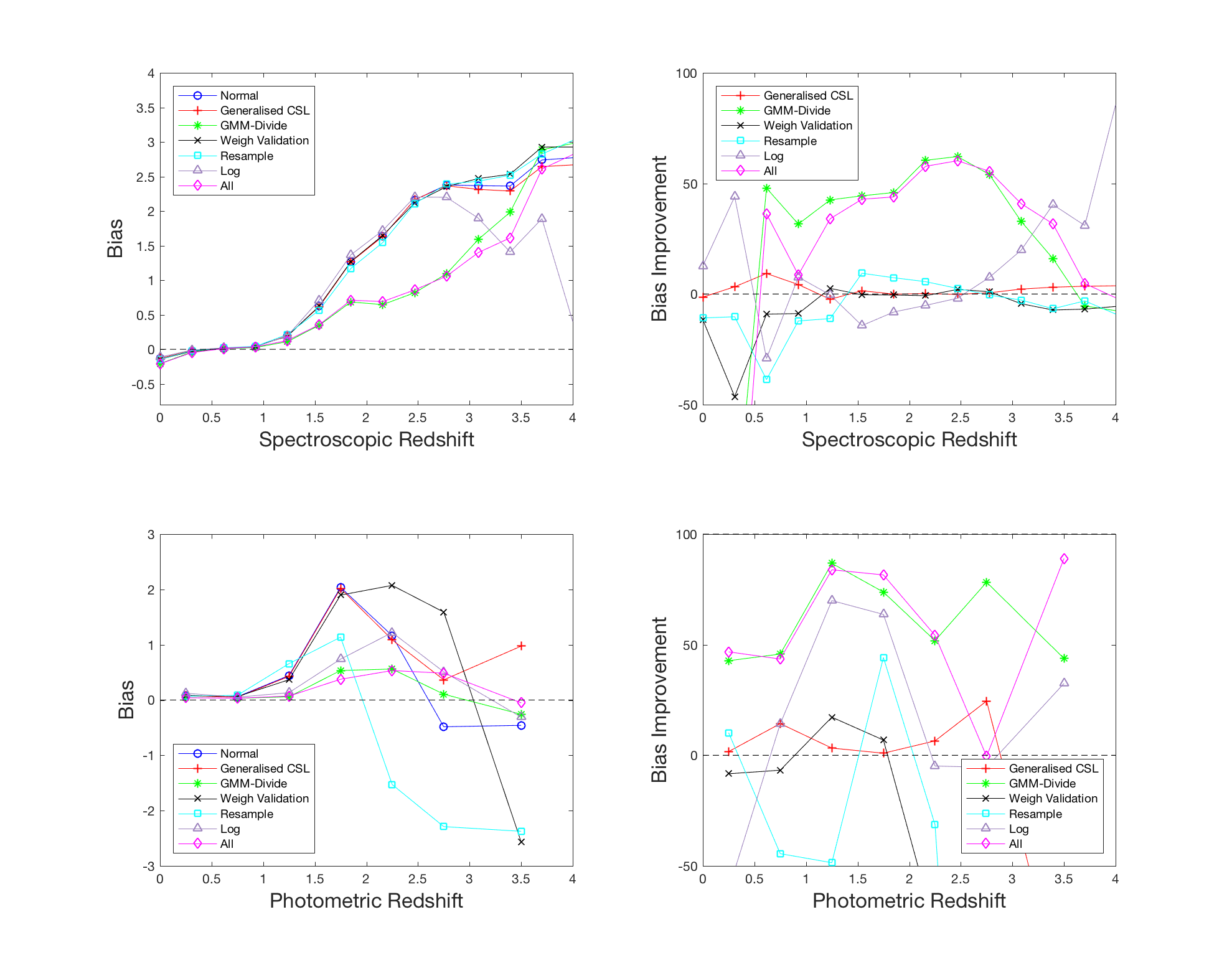
Figure 9: Bias on photometric redshift estimation (left column), and improvement in bias (right column) compared with ‘Normal’; 0 percent is no change in bias and 100 percent is complete removal of bias. Top row shows the results as a function of spectroscopic redshift, bottom row shows as a function of predicted photometric redshift.

4.2 Quality of Probability Distributions

Probability Integral Transform (PIT) plots can be used to compare how well calibrated these pdfs are (D’Isanto & Polsterer, 2018). The plot essentially shows a histogram of cumulative distribution function values at the spectroscopic redshift (e.g. for each galaxy calculate what fraction of the pdf is less than the true value, and plot a histogram of these values). Figure 10 shows the PIT plot for all $z>1$ test data, for both ‘Normal’ and ‘All’. The asymmetric ‘U’ shapes show that the pdfs are slightly over-narrow and biased - but the fact that the ‘All’ curve is closer to a flat line (which would correspond an unbiased pdf) shows the quality of the pdfs has indeed been improved at high redshift. For $z<1$ the PIT plots for ‘Normal’ and ‘All’ are essentially identical.

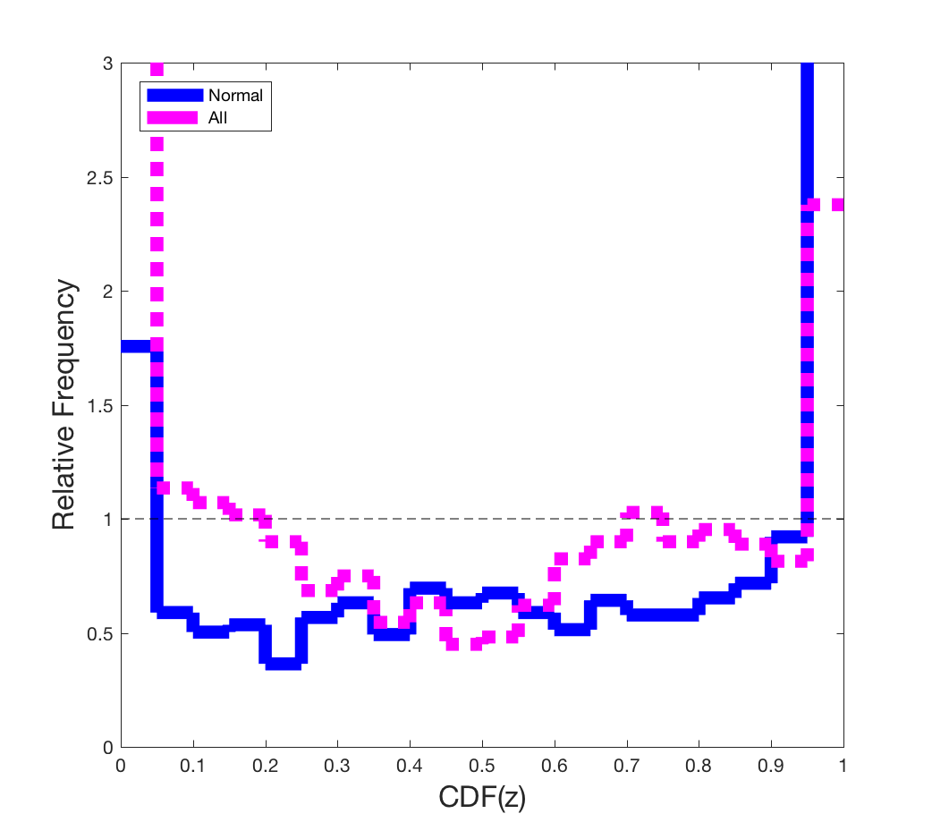
Figure 10: PIT plot for all the test data for ‘Normal’, and ‘All’ methods for photometric redshifts $z>1$. Probability distributions are perfectly calibrated if they lie on the horizontal dashed line.

4.3 Population Redshift Distribution

Finally we plot the summed probability distributions for both ‘Normal’ and ‘All’ to reconstruct estimates of redshift distributions for the test data in figure 11. Both ‘Normal’ and ‘All’ get the lower redshift ‘hump’ correct, but both struggle to identify the higher redshift hump. This is not surprising, given the training data, but it does show that using ‘All’ does manage to $\sim$triple the estimated number of high redshift galaxies, even if this estimate is still below the true number.

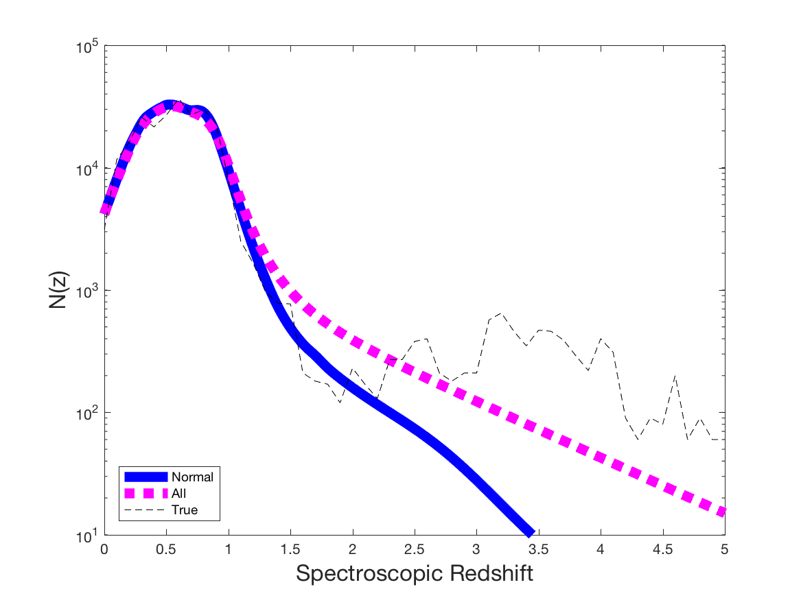
Figure 11: The true underlying redshift distribution (black dashed line), and the stacked pdfs from the a) ’Normal’ (full blue line) and b) ’All’ (dotted magenta line) methods. It can be seen that ’All’ better captures the high redshift distribution.

5 Discussion

Our results show that it is possible to obtain significant improvements to the performance of GPz with comparatively little input (and no extra data), taking into account the differences in colour-magnitude distribution of the training and test data. Although we have discussed in the context of GPz, these methods could be easily extended to any other ML photo-z code. In particular GMM-Divide is easily implemented and gives large improvements, and may be particularly valuable for Euclid and Rubin, where there will be billions of sources, and colour-magnitude space could be profitably split up into hundreds of sections, each still containing $\sim 10^{5}-10^{7}$ galaxies. The methods described here could also be combined with the pdf post-processing method described in Gomes et al. (2018).

Improvements at higher redshifts seem to largely come from ‘Divide’ (modelling different parts of colour-magnitude space separately based on a GMM). This is likely because the ‘Divide’ method identifies a population that corresponds to higher-redshift galaxies. Because each population gets the same share of basis functions, this population gets more basis functions than it normally would in the straightforward implementation of GPz, and can be modelled more accurately. The lower-redshift sources get fewer basis functions than they otherwise would, but still get high performance, as they were only getting a large number of basis functions as it was where the bulk of the data was. An interesting comparison for future analyses where x-ray and/or radio data was available might be to compare the merits and demerits of unsupervised divisions like that discussed in this work, versus cuts explicitly designed to separate AGN and non-AGN.

Resample most improved the RMSE and FR15, but adversely affects the bias. Weight Validation was the best at improving bias. Using ‘Divide’, ‘Resample’ and ‘Weight Validation’ together (‘All’) thus seemed the best way to improve both bias, scatter, and behaviour across all redshifts, and this is borne out by the ‘All’ results for figure 9.

Modelling $\mathrm{log}(z)$ successfully avoids negative redshifts, but typically led to poorer results. It also to some degree pushes the issues at $z=0$ to $z=\infty$; galaxies up-scattered to high $\mathrm{log}(z)$ end up with predicted redshifts in the hundreds. If choosing to keep with modelling $z$ rather than $\mathrm{log}(z)$ it, as discussed, can be tempting to simply ‘cut off’ the negative probability (e.g. declare the final pdf for the galaxy’s redshift to be a Gaussian multiplied by a step-function). This can be an acceptable solution depending on science goals, but as discussed it does have the unfortunate feature of biasing results near $z=0$ e.g. making that cut forces the redshifts to be over estimated. This can be overcome if one requires the whole redshift distribution; some galaxies being assigned negative redshifts can be accepted, and then accounted for when finding the redshift probability distribution for the whole population e.g. with a hierarchical Bayesian model as per FRANKEN-Z (Speagle et al., in prep.).

Figure 10 suggests that ‘All’ improves the calibration of the redshift pdfs for $z>1$. As noted however the asymmetric ‘U’ shapes show that the pdfs are generally slightly too narrow. Having accurate pdfs (as opposed to simply point estimates) is essential for many applications, including luminosity functions e.g. López-Sanjuan et al. (2017). More generally at high redshift it is sometimes found that template-fitting methods can under-estimate uncertainty (Dahlen et al., 2013; Salvato et al., 2019), with machine learning methods usually producing more realistic pdfs (e.g. Brescia et al., 2019).

5.1 Comparison to Template Based Methods

The main focus of this paper is to identify how best to augment machine learning based photo-z’s, but it is nonetheless instructive to see how our ML-based predictions compare to template-based methods. In Figure 12 we show how our ‘Normal’ and ‘All’ photo-z’s compare to the template-based photo-z’s calculated in Adams et al. (2020) using LePhare (Arnouts et al., 1999; Ilbert et al., 2006); it can be seen that the ML and the template-based methods each out-perform the other for different galaxies. In particular it can be seen that typically the template-based method is better when GPz is in the extrapolative regime (i.e. where there is little or no training data). The variance in GPz has three components; $\nu$ (uncertainty from lack of data), $\beta^{-1}_{\star}$ (uncertainty from output noise e.g. galaxies with different redshifts for the same magnitudes) and $\gamma$ (uncertainty from input noise e.g. uncertainty on the magnitudes). The extrapolative uncertainty $\nu$ is typically underestimated (furthermore the transition is smooth with no clear boundary) so we define predictions to be extrapolative if $\nu>0.1\times(\beta^{-1}_{\star}+\gamma)$, see Hatfield et al. (2020). This classification can be used to construct a ‘Combined’ photo-z estimate by using the GPz ‘All’ prediction if GPz is in the interpolative regime, and the LePhare photo-z if GPz is in the extrapolative regime. In Figure 13 we show the bias of the ‘Combined’ method compared with the ML and template based methods, demonstrating that the ‘Combined’ approach as expected outperforms the individual approaches. For the data sets used here, 4 percent of the test data is in the extrapolative regime, although this fraction typically will vary depending on training and test data used.

Euclid and Rubin photometry will cover similar wavelengths to this study, over much larger areas (Rhodes et al., 2017). Future work will test these methods on the Euclid and Rubin data challenges, combining the pdfs constructed here with template based pdfs using both the interpolative/extrapolative method described here, and the Hierarchical Bayesian Model approach of Duncan et al. (2018).

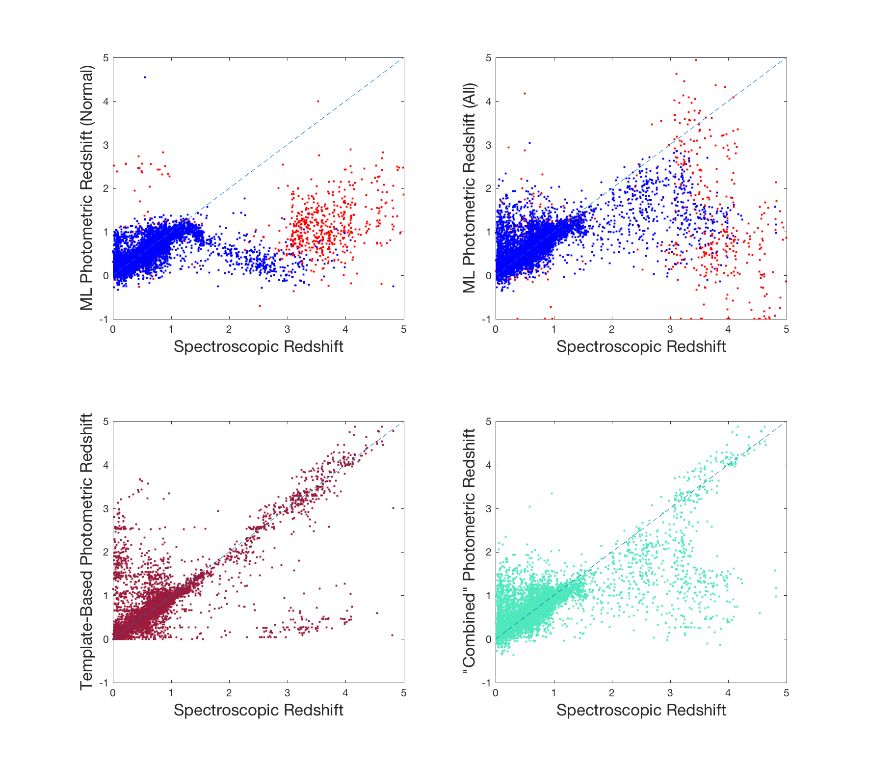
Figure 12: Comparison of ML and template methods. Top left: Our ‘Normal’ ML predictions. Top right: Our ‘All’ ML predictions. Bottom left: The template based predictions of Adams et al. (2020). Bottom right: The ‘Combined’ predictions that incorporate both the ML and the template based methods. For the plots in the top row, blue indicates galaxies in the interpolative regions of colour-magnitude space, and red those in the extrapolative regions.

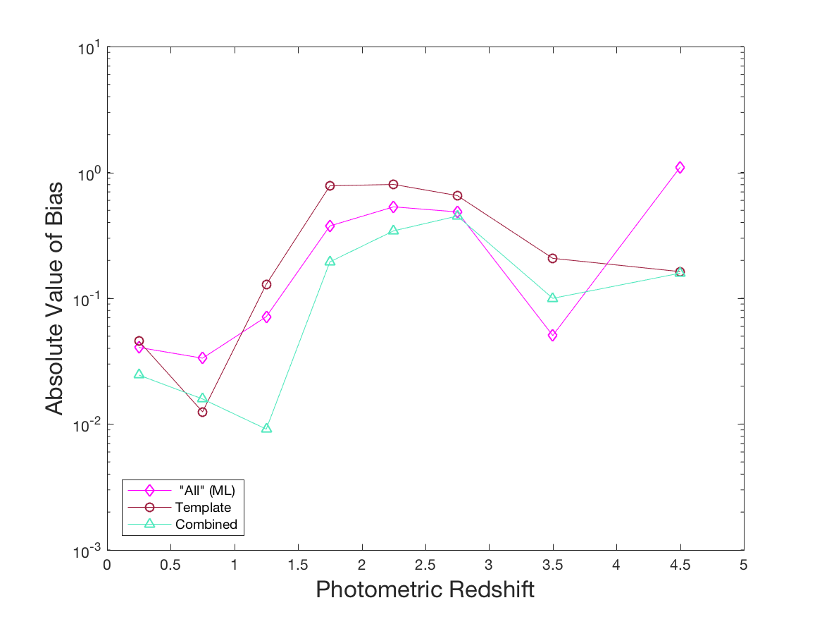
Figure 13: Absolute bias as a function of photometric redshift for a) our ‘All’ ML photo-z’s, b) the Adams et al. (2020) template-based photo-z’s and c) the ‘Combined’ values.

6 Conclusions

In this work we began by constructing mock training and test data sets from CFHT, VISTA, and HSC data, both with spectroscopic redshifts, but with different colour and redshift distributions. This mimics the real issue of spectroscopic training sets having a different colour-magnitude distribution to the target distribution. We then discuss and illustrate several ways of using a combination of GMMs and the machine learning photometric redshift code GPz to obtain improved results over the baseline performance: i) weighting the data appropriately for the colour-magnitude distribution differences, ii) modelling different populations separately, iii) using resampling methods and iv) making the validation data closer to the test data. We compare various metrics from the different methods, finding that respectable improvements in bias at higher redshifts ($z\gtrsim 1.5$) can be achieved with these relatively simple methods (and with no additional training data). In particular, modelling different parts of colour-magnitude space separately (‘Divide’), Resampling, and weighting the validation data to look more like the test data seem to be the most effective and practical methods. These methods worked well even without removing AGN from the samples.

The key conclusions of this work are:

• Weighting schemes that take into account the different colour-magnitude distributions of galaxies in the training and test sets can reduce some of the bias in redshift estimation, particularly at high redshift (without any additional data)

• Using GMMs can help speed up photometric redshift calculation and give improved precision for machine learning based photometric redshift calculation

Data Availability

The derived data generated in this research will be shared on reasonable request to the corresponding author.

References

- Abdalla et al. (2011) Abdalla F. B., Banerji M., Lahav O., Rashkov V., 2011, Monthly Notices of the Royal Astronomical Society, 417, 1891
- Adams et al. (2020) Adams N. J., Bowler R. A. A., Jarvis M. J., Häußler B., McLure R. J., Bunker A., Dunlop J. S., Verma A., 2020, Monthly Notices of the Royal Astronomical Society, 494, 1771
- Aihara et al. (2017) Aihara H. et al., 2017, eprint arXiv:1702.08449, 70
- Alam et al. (2015) Alam S. et al., 2015, The Astrophysical Journal Supplement Series, 219, 12
- Almosallam (2017) Almosallam I., 2017, PhD thesis, University of Oxford
- Almosallam et al. (2016a) Almosallam I. A., Jarvis M. J., Roberts S. J., 2016a, Monthly Notices of the Royal Astronomical Society, 462, 726
- Almosallam et al. (2016b) Almosallam I. A., Lindsay S. N., Jarvis M. J., Roberts S. J., 2016b, Monthly Notices of the Royal Astronomical Society, 455, 2387
- Arnouts et al. (1999) Arnouts S., Cristiani S., Moscardini L., Matarrese S., Lucchin F., Fontana A., Giallongo E., 1999, Monthly Notices of the Royal Astronomical Society, 310, 540
- Baldry et al. (2010) Baldry I. K. et al., 2010, Monthly Notices of the Royal Astronomical Society, 404, 86
- Banerji et al. (2008) Banerji M., Abdalla F. B., Lahav O., Lin H., 2008, Monthly Notices of the Royal Astronomical Society, 386, 1219
- Beck et al. (2017) Beck R. et al., 2017, Monthly Notices of the Royal Astronomical Society, Volume 468, Issue 4, p.4323-4339, 468, 4323
- Bell & de Jong (2001) Bell E. F., de Jong R. S., 2001, The Astrophysical Journal, 550, 212
- Benitez et al. (2004) Benitez N. et al., 2004, The Astrophysical Journal Supplement Series, 150, 1
- Benitez & Narciso (1998) Benitez N., Narciso, 1998, The Astrophysical Journal, 536, 571
- Bertin (2011) Bertin E., 2011, Automated Morphometry with SExtractor and PSFEx, Vol. 442. Astronomical Society of the Pacific (ASP), p. 435
- Bonfield et al. (2010) Bonfield D. G., Sun Y., Davey N., Jarvis M. J., Abdalla F. B., Banerji M., Adams R. G., 2010, Monthly Notices of the Royal Astronomical Society, no
- Bowler et al. (2020) Bowler R. A. A., Jarvis M. J., Dunlop J. S., McLure R. J., McLeod D. J., Adams N. J., Milvang-Jensen B., McCracken H. J., 2020, Monthly Notices of the Royal Astronomical Society, 493, 2059
- Brammer et al. (2008) Brammer G. B., van Dokkum P. G., Coppi P., 2008, The Astrophysical Journal, 686, 1503
- Brescia et al. (2019) Brescia M., Salvato M., Cavuoti S., Ananna T. T., Riccio G., LaMassa S. M., Urry C. M., Longo G., 2019, Monthly Notices of the Royal Astronomical Society, 489, 663
- Buchner et al. (2015) Buchner J. et al., 2015, ApJ, 802, 89
- Carrasco Kind & Brunner (2013) Carrasco Kind M., Brunner R. J., 2013, Monthly Notices of the Royal Astronomical Society, 432, 1483
- Cavuoti et al. (2017) Cavuoti S., Amaro V., Brescia M., Vellucci C., Tortora C., Longo G., 2017, Monthly Notices of the Royal Astronomical Society, 465, 1959
- Chen et al. (2018) Chen C. T. J. et al., 2018, MNRAS, 478, 2132
- Cheng et al. (2020) Cheng T.-Y., Li N., Conselice C. J., Aragón-Salamanca A., Dye S., Metcalf R. B., 2020, Monthly Notices of the Royal Astronomical Society
- Coe et al. (2006) Coe D., Benitez N., Sanchez S. F., Jee M., Bouwens R., Ford H., 2006, The Astronomical Journal, Volume 132, Issue 2, pp. 926-959., 132, 926
- Coil et al. (2011) Coil A. L. et al., 2011, The Astrophysical Journal, 741, 8
- Collaboration et al. (2009) Collaboration L. S. et al., 2009, eprint arXiv:0912.0201
- Collister & Lahav (2004) Collister A. A., Lahav O., 2004, Publications of the Astronomical Society of the Pacific, 116, 345
- Cool et al. (2013) Cool R. J. et al., 2013, The Astrophysical Journal, 767, 118
- Dahlen et al. (2013) Dahlen T. et al., 2013, The Astrophysical Journal, 775, 93
- D’Isanto & Polsterer (2018) D’Isanto A., Polsterer K. L., 2018, Astronomy & Astrophysics, 609, A111
- Duncan et al. (2018) Duncan K. J. et al., 2018, Monthly Notices of the Royal Astronomical Society, 473, 2655
- Feldmann et al. (2006) Feldmann R. et al., 2006, Monthly Notices of the Royal Astronomical Society, Volume 372, Issue 2, pp. 565-577., 372, 565
- Fernandez‐Soto et al. (2001) Fernandez‐Soto A., Lanzetta K. M., Chen H.-W., Pascarelle S. M., Yahata N., 2001, The Astrophysical Journal Supplement Series, 135, 41
- Fotopoulou & Paltani (2018) Fotopoulou S., Paltani S., 2018, A&A, 619, A14
- Gomes et al. (2018) Gomes Z., Jarvis M. J., Almosallam I. A., Roberts S. J., 2018, Monthly Notices of the Royal Astronomical Society, 475, 331
- Hasinger et al. (2018) Hasinger G. et al., 2018, The Astrophysical Journal, 858, 77
- Hatfield et al. (2020) Hatfield P., Rose S., Scott R., Almosallam I., Roberts S., Jarvis M., 2020, IEEE Transactions on Plasma Science, 48, 14
- Hearin et al. (2010) Hearin A. P., Zentner A. R., Ma Z., Huterer D., 2010, The Astrophysical Journal, Volume 720, Issue 2, pp. 1351-1369 (2010)., 720, 1351
- Hildebrandt et al. (2017) Hildebrandt H. et al., 2017, Monthly Notices of the Royal Astronomical Society, 465, 1454
- Hoyle et al. (2018) Hoyle B. et al., 2018, Monthly Notices of the Royal Astronomical Society, 478, 592
- Ilbert et al. (2006) Ilbert O. et al., 2006, Astronomy and Astrophysics, 457, 841
- Jaakkola & Jordan (2000) Jaakkola T. S., Jordan M. I., 2000, Statistics and Computing, 10, 25
- Jarvis et al. (2013) Jarvis M. J. et al., 2013, Monthly Notices of the Royal Astronomical Society, 428, 1281
- Jordan et al. (1999) Jordan M. I., Ghahramani Z., Jaakkola T. S., Saul L. K., 1999, Machine Learning, 37, 183
- Kuhn & Feigelson (2017) Kuhn M. A., Feigelson E. D., 2017, eprint arXiv:1711.11101
- Laigle et al. (2016) Laigle C. et al., 2016, The Astrophysical Journal Supplement Series, 224, 24
- Laureijs et al. (2011) Laureijs R. et al., 2011, eprint arXiv:1110.3193
- Le Fèvre et al. (2013) Le Fèvre O. et al., 2013, Astronomy & Astrophysics, 559, A14
- Leistedt et al. (2016) Leistedt B., Mortlock D. J., Peiris H. V., Leistedt B., Mortlock D. J., Peiris H. V., 2016, MNRAS, 460, 4258
- Lilly et al. (2009) Lilly S. J. et al., 2009, The Astrophysical Journal Supplement Series, 184, 218
- Lima et al. (2008) Lima M. et al., 2008, MNRAS, 390, 118
- López-Sanjuan et al. (2017) López-Sanjuan C. et al., 2017, Astronomy & Astrophysics, 599, A62
- Lupton et al. (1999) Lupton R., Gunn J., Szalay A., Lupton R. H., Gunn J. E., Szalay A. S., 1999, AJ, 118, 1406
- Marchesi et al. (2016) Marchesi S. et al., 2016, The Astrophysical Journal, 817, 34
- Masters et al. (2015) Masters D. et al., 2015, ApJ, 813, 53
- McCracken et al. (2012) McCracken H. J. et al., 2012, Astronomy & Astrophysics, 544, A156
- McLure et al. (2018) McLure R. J. et al., 2018, Monthly Notices of the Royal Astronomical Society, 479, 25
- Momcheva et al. (2016) Momcheva I. G. et al., 2016, The Astrophysical Journal Supplement Series, 225, 27
- Norris et al. (2019) Norris R. P. et al., 2019, Publications of the Astronomical Society of the Pacific, 131, 108004
- Peng & Bai (2019) Peng H., Bai X., 2019, Astrodynamics, 1
- Pentericci et al. (2018) Pentericci L. et al., 2018, Astronomy & Astrophysics, 616, A174
- Rasmussen & Williams (2006) Rasmussen C. E., Williams C. K. I., 2006, Gaussian processes for machine learning. MIT Press, p. 248
- Rhodes et al. (2017) Rhodes J. et al., 2017
- Sadeh et al. (2016) Sadeh I., Abdalla F. B., Lahav O., 2016, Publications of the Astronomical Society of the Pacific, 128, 104502
- Salvato et al. (2019) Salvato M., Ilbert O., Hoyle B., 2019, Nature Astronomy, 3, 212
- Sawicki et al. (2019) Sawicki M. et al., 2019, Monthly Notices of the Royal Astronomical Society, 489, 5202
- Schmidt et al. (2020) Schmidt S. J. et al., 2020
- Silverman et al. (2015) Silverman J. D. et al., 2015, The Astrophysical Journal Supplement Series, 220, 12
- Skelton et al. (2014) Skelton R. E. et al., 2014, The Astrophysical Journal Supplement Series, 214, 24