Practical and Parallelizable Algorithms for Non-Monotone Submodular Maximization with Size Constraint

Abstract

We present combinatorial and parallelizable algorithms for maximization of a submodular function, not necessarily monotone, with respect to a size constraint. We improve the best approximation factor achieved by an algorithm that has optimal adaptivity and nearly optimal query complexity to $0.193-\varepsilon$. The conference version of this work mistakenly employed a subroutine that does not work for non-monotone, submodular functions. In this version, we propose a fixed and improved subroutine to add a set with high average marginal gain, ThreshSeq, which returns a solution in $O\left(\log(n)\right)$ adaptive rounds with high probability. Moreover, we provide two approximation algorithms. The first has approximation ratio $1/6-\varepsilon$, adaptivity $O(\log(n))$, and query complexity $O(n\log(k))$, while the second has approximation ratio $0.193-\varepsilon$, adaptivity $O(\log^{2}(n))$, and query complexity $O(n\log(k))$. Our algorithms are empirically validated to use a low number of adaptive rounds and total queries while obtaining solutions with high objective value in comparison with state-of-the-art approximation algorithms, including continuous algorithms that use the multilinear extension.

1 Introduction

A nonnegative set function $f:2^{\mathcal{N}}\to\mathbb{R}^{+}$, defined on all subsets of a ground set $\mathcal{N}$ of size $n$, is submodular if for all $A,B\subseteq\mathcal{N}$, $f(A)+f(B)\geq f(A\cup B)+f(A\cap B)$. Submodular set functions naturally arise in many learning applications, including data summarization (?, ?, ?, ?), viral marketing (?, ?), and recommendation systems (?). Some applications yield submodular functions that are not monotone (a set function is monotone if $A\subseteq B$ implies $f(A)\leq f(B)$): for example, image summarization with diversity (?) or revenue maximization on a social network (?). In this work, we study the maximization of a (not necessarily monotone) submodular function subject to a cardinality constraint; that is, given submodular function $f$ and integer $k$, determine $\arg\,\max_{|S|\leq k}f(S)$ (SMCC). Access to $f$ is provided through a value query oracle, which when queried with the set $S$ returns the value $f(S)$.

As the amount of data in applications has exhibited exponential growth in recent years (e.g. the growth of social networks (?) or genomic data (?)), it is necessary to design algorithms for SMCC that can scale to these large datasets. One aspect of algorithmic efficiency is the query complexity, the total number of queries to the oracle for $f$; since evaluation of $f$ is often expensive, the queries to $f$ often dominate the runtime of an algorithm. In addition to low query complexity, it is necessary to design algorithms that parallelize well to take advantage of modern computer architectures. To quantify the degree of parallelizability of an algorithm, the adaptivity or adaptive complexity of an algorithm is the minimum number of sequential rounds such that in each round the algorithm makes $O(\text{poly}(n))$ independent queries to the evaluation oracle. The lower the adaptive complexity of an algorithm, the more suited the algorithm is to parallelization, as within each adaptive round, the queries to $f$ are independent and may be easily parallelized.

The design of algorithms with nontrivial adaptivity for SMCC when $f$ is monotone was initiated by ?’s (?), who also prove a lower bound of $\Omega(\log(n)/\log\log(n))$ adaptive rounds to achieve a constant approximation ratio. Recently, much work has focused on the design of adaptive algorithms for SMCC with (not necessarily monotone) submodular functions, as summarized in Table 1. However, although many algorithms with low adaptivity have been proposed, most of these algorithms exhibit at least a quadratic dependence of the query complexity on the size $n$ of the ground set, for $k=\Omega(n)$. For many applications, instances have grown too large for quadratic query complexity to be practical. Therefore, it is necessary to design adaptive algorithms that also have nearly linear query complexity. An algorithm in prior literature that meets this requirement is the algorithm developed by ?’s (?), which has $O(n\log(k))$ query complexity and $O(\log(n))$ adaptivity. However, the approximation ratio stated in ?’s (?) for this algorithm does not hold, as discussed in Section 1.1 and Appendix B.

Table 1: Adaptive algorithms for SMCC where objective $f$ is not necessarily monotone.

Reference	Approximation	Adaptivity	Queries
?’s (?)	$1/e-\varepsilon$	$O(k)$	${O(n)}$
?’s (?)	$1/(2e)-\varepsilon$	$O\left(\log^{2}(n)\right)$	$O\left(OPT^{2}n\log^{2}(n)\log(k)\right)$
?’s (?)	$3-2\sqrt{2}-\varepsilon$	$O(\log^{2}(n))$	$O\left(nk^{4}\log^{2}(n)\right)$
?’s (?)	$1/e-\varepsilon$	${O(\log(n))}$	$O\left(nk^{2}\log^{2}(n)\right)$
?’s (?)	$0.039-\varepsilon$ $\dagger$	${O(\log(n))}$	${O(n\log(k))}$
?’s (?)	$0.172-\varepsilon$	$O\left(\log(n)\right)$ $O\left(\log(n)\log(k)\right)$	$O\left(nk\log(n)\log(k)\right)$ $O\left(n\log(n)\log^{2}(k)\right)$
Theorem 7 (AST)	$1/6-\varepsilon$	${O(\log(n))}$	${O(n\log(k))}$
Theorem 8 (ATG)	$0.193-\varepsilon$	$O(\log(n)\log(k))$	${O(n\log(k))}$

• The approximation ratio of this algorithm does not hold, and is discussed in Appendix B.

Contributions. In this work, we propose two fast, combinatorial algorithms for SMCC: the $(1/6-\varepsilon)$-approximation algorithm AdaptiveSimpleThreshold (AST) with adaptivity $O(\log(n))$ and query complexity $O(n\log(k))$; and the $(0.193-\varepsilon)$-approximation algorithm AdaptiveThresholdGreedy (ATG) with adaptivity $O(\log(n)\log(k))$ and query complexity $O(n\log(k))$.

The above algorithms both employ a lowly-adaptive subroutine to add multiple elements that satisfy a given marginal gain, on average. The conference version (?) of this paper used the Threshold-Sampling subroutine of ?’s (?, ?) for this purpose. However, the theoretical guarantee (Lemma 2.3 of ?’s (?)) for non-monotone functions does not hold, as discussed further. In Appendix B, we give a counterexample to the performance guarantee of Threshold-Sampling. In this version, we introduce a new threshold subroutine ThreshSeq, which not only fixes the problem that Threshold-Sampling faced, but achieves its guarantees with high probability as opposed to in expectation; the high probability guarantees simplify the analysis of our approximation algorithms that rely upon the ThreshSeq subroutine.

Our algorithm AST uses a double-threshold procedure to obtain its ratio of $1/6-\varepsilon$. Our second algorithm ATG is a low-adaptivity modification of the algorithm of ?’s (?), for which we improve the ratio from $1/6$ to $\approx$0.193 through a novel analysis. Both of our algorithms use the low-adaptivity, threshold sampling procedure ThreshSeq and a subroutine for unconstrained maximization of a submodular function (?, ?) as components. More details are given in the related work discussion below and in Section 4.

The new ThreshSeq does not rely on sampling to achieve concentration bounds, which significantly improves the practical efficiency of our algorithms over the conference version. Empirically, we demonstrate that both of our algorithms achieve superior objective value to current state-of-the-art algorithms while using a small number of queries and adaptive rounds on two applications of SMCC.

1.1 Related Work

Theshold Procedures. A recurring subproblem of SMCC (and other submodular optimization problems) is to add all elements of the ground set that give a marginal gain of at least $\tau$, for some constant threshold $\tau$. To solve this subproblem, the algorithm Threshold-Sampling is proposed in ?’s (?) for monotone submodular functions and applied in ?’s (?) and the conference version of this work (?) as subroutines for non-monotone SMCC. However, theoretical guarantee (Lemma 2.3 of ?’s (?)) does not hold when the objective function is non-monotone. Counterexamples and pseudocode for Threshold-Sampling are given in Appendix B.

Two alternative solutions to the non-monotone threshold problem were proposed in ?’s (?) for the case of non-monotone, submodular maximization subject to a knapsack constraint. Due to the complexity of the constraints, the thresholding procedures in ?’s (?) have a high time complexity and require $O\left(n^{2}\right)$ query calls within one iteration even when restricted to size constraint. Although a variant with binary search is proposed to get fewer queries, the sequential binary search worsens the adaptivity of the algorithm.

In this work, we propose the ThreshSeq algorithm (Section 2) that fixes the problems of Threshold-Sampling and runs in linear time in the size $n$ of the ground set in $O(\log n)$ rounds. We solve these problems by bifurcating the solution found by the algorithm into two sets: an auxilliary set $A$ separate from the solution set $A^{\prime}$ found by ThreshSeq; the algorithm maintains that $A^{\prime}\subseteq A$, and the larger set is used for filtering from the ground set, while the smaller set maintains desired bounds on the average marginal gain.

Algorithms with Low Adaptive Complexity. Since the study of parallelizable algorithms for submodular optimization was initiated by ?’s (?), there have been a number of $O(\log n)$-adaptive algorithms designed for SMCC. When $f$ is monotone, adaptive algorithms that obtain the optimal ratio (?) of $1-1/e-\varepsilon$ have been designed by ?’s (?, ?, ?, ?). Of these, the algorithm of ?’s (?) also has the state-of-the-art sublinear adapativity and linear query complexity.

However, when the function $f$ is not monotone, the best approximation ratio with polynomial query complexity for SMCC is unknown, but falls within the range $[0.385,0.491]$ (?, ?). For SMCC, algorithms with nearly optimal adaptivity have been designed by ?’s (?, ?, ?, ?, ?); for the query complexity and approximation factors of these algorithms, see Table 1. Of these, the best approximation ratio of $(1/e-\varepsilon)\approx 0.368$ is obtained by the algorithm of ?’s (?). However, this algorithm requires access to an oracle for the gradient of the continuous extension of a submodular set function, which requires $\Omega(nk^{2}\log^{2}(n))$ queries to sufficiently approximate; the practical performance of the algorithm of ?’s (?) is investigated in our empirical evaluation of Section 5. Other than the algorithms of ?’s (?) and ?’s (?), all parallelizable algorithms exhibit a runtime of at least quadratic dependence on $n$, in contrast, our algorithms have query complexity of $O(n\log k)$ and have $O(\log n)$ or $O(\log^{2}n)$ adaptivity.

After the conference version (?) of this paper, ?’s (?) proposed a parallelizable algorithm, ParKnapsack, for knapsack constraints, which is the first constant factor approximation with optimal adaptive complexity. In the paper, ParKnapsack is directly applied to cardinality constraints. It achieves a $0.172-\varepsilon$ ratio with two different variants: one has $O\left(\log(n)\right)$ adaptive rounds and $O\left(nk\log(n)\log(k)\right)$ queries; another one has $O\left(\log(n)\log(k)\right)$ adaptive rounds and $O\left(n\log(n)\log^{2}(k)\right)$ queries. Compared to our nearly linear algorithms, the first variant of ParKnapsack requires total queries with more than quadratic dependence on $n$; and the second variant gets a worse approximation ratio and worse number of queries than our algorithm (ATG) with the same adaptivity.

The IteratedGreedy Algorithm. Although the standard greedy algorithm performs arbitrarily badly for SMCC, ?’s (?) showed that multiple repetitions of the greedy algorithm, combined with an approximation for the unconstrained maximization problem, yields an approximation for SMCC. Specifically, ?’s (?) provided the IteratedGreedy algorithm, which achieves an approximation ratio of $1/6$ for SMCC when the $1/2$-approximation of ?’s (?) is used for the unconstrained maximization subproblems. Our algorithm AdaptiveThresholdGreedy uses ThreshSeq combined with the descending thresholds technique of ?’s (?) to obtain an adaptive version of IteratedGreedy, as described in Section 4. Pseudocode for IteratedGreedy is given in Appendix E, where an improved ratio of $\approx$0.193 is proven for this algorithm; we also prove the ratio of nearly $0.193$ for our adaptive algorithm ATG in Section 4.

1.2 Preliminaries

A submodular set function defined on all subsets of ground set $\mathcal{N}$ is denoted by $f$. The marginal gain of adding an element $s$ to a set $S$ is denoted by $\Delta\left(s\,|\,S\right)=f(S\cup\{s\})-f(S)$. Let $\textsc{OPT}=\max_{|S|\leq k}f(S)$. The restriction of $f$ to all subsets of a set $S\subseteq\mathcal{N}$ is denoted by $f\restriction_{S}$. Next, we describe two subproblems both of our algorithms need to solve: namely, unconstrained maximization subproblems and a threshold sampling subproblem. For both of these subproblems, procedures with low adaptivity are needed.

The Unconstrained Maximization Problem. The first subproblem is unconstrained maximization of a submodular function. When the function $f$ is non-monotone, the problem of maximizing $f$ without any constraints is NP-hard (?). Recently, ?’s (?) developed an algorithm that achieves nearly the optimal ratio of $1/2$ with constant adaptivity, as summarized in the following theorem.

Theorem 1 (?’s (?)).

For each $\varepsilon>0$, there is an algorithm that achieves a $(1/2-\varepsilon)$-approximation for unconstrained submodular maximization using $O(\log(1/\varepsilon)/\varepsilon)$ adaptive rounds and $O(n\log^{3}(1/\varepsilon)/\varepsilon^{4})$ evaluation oracle queries.

To achieve the approximation factor listed for our algorithms in Table 1, the algorithm of ?’s (?) is employed for unconstrained maximization subproblems.

The Threshold Problem. The second subproblem is the following:

Definition 2 (Threshold).

Given a threshold $\tau\in\mathbb{R}$ and integer $k$, choose a set $S$ such that 1) $f(S)\geq\tau|S|$; 2) if $|S|<k$, then for any $x\not\in S$, $\Delta\left(x\,|\,S\right)<\tau$.

Algorithms that can use a solution to this subproblem occur frequently, and so multiple algorithms in the literature for this subproblem have been formulated (?, ?, ?, ?). We want a procedure that can solve Threshold with the following three properties: 1) in linear time; 2) in $O(\log n)$ adaptive rounds; 3) the function $f$ is non-monotone.

None of the prior algorithms satisfy our requirements, since the procedures in ?’s (?, ?, ?) only works when the submodular function is monotone; and the two procedures in ?’s (?) have either $O\left(n^{2}\log(n)\right)$ queries or $O\left(\log^{2}(n)\right)$ adaptivity. Moreover, in both ?’s (?) and ?’s (?), the procedures for Threshold only guarantee $\mathbb{E}\left[f(S)\right]\geq\tau|S|$.

In this paper, we propose ThreshSeq, which is linear time and has $O(\log n)$ adaptivity. This algorithm does not exactly solve Threshold; instead, it returns two sets $A^{\prime}\subseteq A$, such that $f(A^{\prime})\geq\tau(1-\varepsilon)|A|$ with high probability; and $\Delta\left(x\,|\,A\right)<\tau$ for all $x\not\in A$, which is enough for our algorithms.

Organization. In Section 2, we introduce our threshold sampling algorithm: ThreshSeq, with detailed analysis in Appendix C. Then, in Sections 3 and 4, we analyze our algorithms using the ThreshSeq and UnconstrainedMax procedures. Our empirical evaluation is reported in Section 5 with more discussions in Appendix G.

2 The ThreshSeq Algorithm

Algorithm 1 A parallelizable threshold algorithm for threshold $\tau$

1:procedure ThreshSeq($f,\mathcal{N},k,\delta,\varepsilon,\tau$)

2:     Input: evaluation oracle $f:2^{\mathcal{N}}\to\mathbb{R}^{+}$, constraint $k$, accuracy $\delta$, error $\varepsilon$, threshold $\tau$

3:     Initialize $A\leftarrow\emptyset$, $A^{\prime}\leftarrow\emptyset$, $V\leftarrow\mathcal{N}$, $\ell=\lceil 4\left(\frac{2}{\varepsilon}\log(n)+\log\left(\frac{n}{\delta}\right)\right)\rceil$

4:     for  $j\leftarrow 1$ to $\ell$ do $\triangleright$ Sequential for loop

5:         Update $V\leftarrow\{x\in V:\Delta\left(x\,|\,A\right)\geq\tau\}$ $\triangleright$ Filtering step w.r.t. $A$

6:         if  $|V|=0$  then

7:              return $A,A^{\prime}$          

8:         $V\leftarrow$ random-permutation$(V)$

9:         $s\leftarrow\min\{k-|A|,|V|\}$

10:         $B[1:s]\leftarrow[\textbf{none},\cdots,\textbf{none}]$

11:         for $i\leftarrow 1$ to $s$ in parallel do $\triangleright$ Parallel gain computation

12:              $T_{i-1}\leftarrow\{v_{1},v_{2},\ldots,v_{i-1}\}$

13:              if $\Delta\left(v_{i}\,|\,A\cup T_{i-1}\right)\geq\tau$ then $B[i]\leftarrow\textbf{true}$

14:              elif $\Delta\left(v_{i}\,|\,A\cup T_{i-1}\right)<0$ then $B[i]\leftarrow\textbf{false}$          

15:         $i^{*}\leftarrow\max\{i:\#\text{{true}s in }B[1:i]\geq(1-\varepsilon)i\}$ $\triangleright$ Detection of good filtering next iteration

16:         $A\leftarrow A\cup T_{i^{*}}$ $\triangleright$ $A$ gets all elements

17:         $A^{\prime}\leftarrow A^{\prime}\cup T_{i^{*}}[\text{where }B\not=\textbf{false}]$ $\triangleright$ $A^{\prime}$ only gets nonnegative-gain elements

18:         if  $|A|=k$  then

19:              return $A,A^{\prime}$               

20:     return failure

In this section, we introduce the linear and highly parallelizable threshold sampling algorithm ThreshSeq (Alg. 1). This algorithm has logarithmic adaptive rounds and linear query calls with high probability. Rather than directly solving Threshold, it returns two sets $A^{\prime}\subseteq A$ such that the average marginal gain of elements of $A^{\prime}$ is exactly larger than the threshold with a small error rate, and $\Delta\left(x\,|\,A\right)<\tau$ for any $x\not\in A$.

Overview of Algorithm. To obtain large sequences of elements with gains above $\tau$, the machinery of existing monotone algorithms (?, ?) is adopted. These algorithms work by adaptively adding sequences of elements to a set $A$, where the sequence has been checked in parallel to have at most an $\varepsilon$ fraction of the sequence failing the marginal gain condition. A uniformly random permutation of elements is considered, where the average marginal gain being below $\tau$ is detected by a high proportion of failures in the sequence, which leads to a large number of elements being filtered out at the next iteration.

The intuitive reason why this does not directly work for non-monotone functions (i.e. $A$ is not a solution to Threshold) is the same reason why Threshold-Sampling of ?’s (?, ?) fails: if one of the elements added fails the marginal gain condition, it may do so arbitrarily badly and have a large negative marginal gain. Moreover, one cannot simply exclude such elements from consideration, because they are needed to ensure the filtering step at the next iteration will discard a large enough fraction of elements. Our solution is to keep these elements in the set $A$ which is used for filtering, but only include those elements with a nonnegative marginal gain in the candidate solution set $A^{\prime}$. The membership of $A^{\prime}$ is known since the gain of every element was computed in parallel. Moreover, $|A^{\prime}|\geq(1-\varepsilon)|A|$, which gives the needed relationship on the average marginal gain of each element of $A^{\prime}$.

We prove the following theorem concerning the performance of ThreshSeq.

Theorem 3.

Let $(f,k)$ be an instance of SMCC. For any constant $\varepsilon$, the algorithm ThreshSeq outputs $A^{\prime}\subseteq A\subseteq\mathcal{N}$ such that the following properties hold: 1) The algorithm succeeds with probability at least $1-\delta/n$. 2) There are $O\left(n/\varepsilon\right)$ oracle queries in expectation and $O\left(\log(n/\delta)/\varepsilon\right)$ adaptive rounds. 3) It holds that $f(A^{\prime})\geq(1-\varepsilon)\tau|A|$. If $|A|<k$, then $\Delta\left(x\,|\,A\right)<\tau$ for all $x\in\mathcal{N}$. 4) It also holds that $f(A^{\prime})\geq f(A)$ and $|A^{\prime}|\geq(1-\varepsilon)|A|$

A downside of this bifurcated approach is that a downstream algorithm receives two sets $A,A^{\prime}$ instead of one from ThreshSeq and must be able to handle the fact that the gain of an element to the solution $A^{\prime}$ may be greater than $\tau$. Fortunately, our approximation algorithms below can easily handle this restriction.

Overview of Proof. The proof of this theorem mainly focuses on two questions: 1) if a constant fraction of elements can be filtered out at any iteration with a high probability; 2) if the two sets returned solve Threshold indirectly. In Lemma 4, it is certified that the number of elements being deleted in the next iteration monotonously increases from 0 to $|V|$ as the size of the selected set increases. Then, by probability lemma and concentration bounds, Lemma 5 answers the first question. Furthermore, with enough iterations, the candidate set $V$ becomes empty at some point with a high probability. Also, since the size of the candidate set $|V|$ exponentially decreases, intuitively, with logarithmic iterations, the total queries is linear. As for Threshold, it is obvious that the second property holds with set $A$; and, by discarding the elements with negative gains in $A$, the gains of the rest elements increase and follow the first property of Threshold.

Proof of Theorem 3.

Success Probability. The algorithm succeeds if $|V|=0$ or $|A|=k$ at termination. If we can filter out a constant fraction of $V$ or select a subset with $k-|A|$ elements at any iteration with a constant probability, then, with enough iterations, the algorithm successfully terminates with a high probability. The proofs of lemmas in this section are given in Appendix C.

Lemma 4.

After random-permutation on Line 8, let $S_{i}=\{x\in V:\Delta\left(x\,|\,A\cup T_{i}\right)<\tau\}$. It holds that $|S_{0}|=0$, $|S_{|V|}|=|V|$, and $|S_{i-1}|\leq|S_{i}|$.

From Lemma 4, there exists a point $t$ such that $t=\min\{i:|S_{i}|\geq\varepsilon|V|/2\}$, where the next iteration filters out more than $\varepsilon/2$-fraction of elements if $i^{*}\geq t$. Intuitively, when $i\leq t$, there is a high probability that the portion of trues in $B[1:i]$ exceeds $1-\varepsilon$. The following lemma is provided.

Lemma 5.

It holds that $Pr\left(i^{*}<\min\{s,t\}\right)\leq 1/2$.

Suppose the algorithm does not stop when $|A|=0$. If so, in the following iterations, it always holds that $s=0$ and $T_{i^{*}}=\emptyset$. Lemma 5 still holds in this case. If there are at least $m=\lceil\log_{1-\varepsilon/2}(1/n)\rceil$ iterations that $i^{*}\geq\min\{s,t\}$, the algorithm terminate successfully. Define such iteration as a successful iteration. Then, the number of successful iterations is a sum of dependent Bernoulli random variables. With probability lemma and Chernoff bounds, the algorithms is proven to be succeed with probability at least $1-\delta/n$ in Appendix C.

Objective Values and Marginal Gains. If $|A|<k$, it holds that algorithm terminates with $|V|=0$. So, for any $x\in\mathcal{N}$, there exists an iteration $j_{(x)}+1$ such that $x$ is filtered out at iteration $j_{(x)}+1$. Then, due to submodularity, it holds that $\Delta\left(x\,|\,A\right)\leq\Delta\left(x\,|\,A_{j_{(x)}}\right)<\tau$.

Lemma 6.

Say an element added to the solution set good if its gain is greater than $\tau$. $A$ and $A^{\prime}$ returned by Algorithm 1 hold the following properties: 1) There are at least $(1-\varepsilon)$-fraction of $A$ that is good. 2) A good element in $A$ is always a good element in $A^{\prime}$. 3) And, any element in $A^{\prime}$ has non-negative marginal gain when added.

Lemma 6 shows the properties of any single element in $A$ and $A^{\prime}$. Since $A^{\prime}$ is a subset of $A$ with all the positive gain elements, it holds that $|A^{\prime}|\geq(1-\varepsilon)|A|$. By deleting an element in a set of sequence, the marginal gains of the other elements is nondecreasing due to the diminishing property of submodular function. For any $x\in A$, let $A_{(x)}$ be a subsequence of $A$ before $x$ is added into $A$. Define $A_{(x)}^{\prime}$ analogously. By Lemma 6, it holds that

$$f(A^{\prime})=\sum_{x\in A^{\prime}}\Delta\left(x\,|\,A_{(x)}^{\prime}\right)\geq\sum_{x\in A^{\prime}}\Delta\left(x\,|\,A_{(x)}\right)+\sum_{x\in A\backslash A^{\prime}}\Delta\left(x\,|\,A_{(x)}\right)\geq f(A),$$

$$f(A^{\prime})=\sum_{x\in A^{\prime}}\Delta\left(x\,|\,A_{(x)}^{\prime}\right)\geq\sum_{x\in A^{\prime},x\text{ is good}}\Delta\left(x\,|\,A_{(x)}^{\prime}\right)\geq(1-\varepsilon)\tau|A|.$$

Adaptivity and Query Complexity. In Alg. 1, the oracle queries occur on Line 5 and 13. Since filtering and inner for loop can be done in parallel, there are constant adaptive rounds in an iteration. Therefore, the adaptivity is $O\left(\ell\right)=O\left(\log(n/\delta)/\varepsilon\right)$.

As for the query complexity, let $V_{j}$ be the set $V$ after filtering on Line 5 in iteration $j$. There are $|V_{j-1}|+1$ and $|V_{j}|+1$ query calls on Line 5 and 13, respectively. Suppose the number of iterations that successfully filter out more than $\varepsilon/2$-fraction of $V$ equals $i$ before current iteration $j$. The size of $|V_{j}|$ can be bounded by $n{(1-\varepsilon/2)}^{i}$. We show that the expected total queries are $O\left(n/\varepsilon\right)$ in Appendix C. ∎

3 The AdaptiveSimpleThreshold Algorithm

Algorithm 2 The AdaptiveSimpleThreshold Algorithm

1:procedure AST($f,\mathcal{N},k,\varepsilon$)

2:     Input: evaluation oracle $f:2^{\mathcal{N}}\to\mathbb{R}^{+}$, constraint $k$, accuracy parameter $\varepsilon>0$

3:     Initialize $M\leftarrow\max_{x\in\mathcal{N}}f(x)$; $c\leftarrow 4+\alpha$, where $\alpha^{-1}$ is ratio of UnconstrainedMax; $\ell\leftarrow\lceil\log_{1-\varepsilon}(1/(ck)))\rceil$

4:     for  $i\leftarrow 0$ to $\ell$ in parallel do

5:         $\tau_{i}\leftarrow M\left(1-\varepsilon\right)^{i}$

6:         $A_{i},A_{i}^{\prime}\leftarrow\textsc{ThreshSeq}\left(f,k,\tau_{i},\varepsilon,1/2\right)$

7:         $B_{i},B_{i}^{\prime}\leftarrow\textsc{ThreshSeq}\left(f\restriction_{\mathcal{N}\setminus A_{i}},k,\tau_{i},\varepsilon,1/2\right)$

8:         $A_{i}^{\prime\prime}\leftarrow\textsc{UnconstrainedMax}(A_{i})$

9:         $C_{i}\leftarrow\arg\,\max\{f(A_{i}^{\prime}),f(B_{i}^{\prime}),f(A_{i}^{\prime\prime})\}$      

10:     return $C\leftarrow\arg\,\max_{i}\{f(C_{i})\}$

In this section, we present the simple algorithm AdaptiveSimpleThreshold (AST, Alg. 2) and show it obtains a ratio of $1/6-\varepsilon$ with nearly optimal query and adaptive complexity. This algorithm relies on running ThreshSeq for a suitably chosen threshold value. A procedure for unconstrained maximization is also required.

Overview of Algorithm. Algorithm AST works as follows. First, the for loop guesses a value of $\tau$ close to $\frac{\textsc{OPT}}{(4+\alpha)k}$, where $1/\alpha$ is the ratio of the algorithm used for the unconstrained maximization subproblem. Next, ThreshSeq is called with parameter $\tau$ to yield set $A$ and $A^{\prime}$; followed by a second call to ThreshSeq with $f$ restricted to $\mathcal{N}\setminus A$ to yield set $B$ and $B^{\prime}$. Next, an unconstrained maximization is performed with $f$ restricted to $A$ to yield set $A^{\prime\prime}$; finally, the best of the three candidate sets $A^{\prime},B^{\prime},A^{\prime\prime}$ is returned.

We prove the following theorem concerning the performance of AST.

Theorem 7.

Suppose there exists an $(1/\alpha)$-approximation for UnconstrainedMax with adaptivity $\Theta$ and query complexity $\Xi$, and let $\varepsilon>0$, $c=4+\alpha$. Then there exists an algorithm for SMCC with expected approximation ratio $c^{-1}-\varepsilon$ with probability at least $1-1/n$, expected query complexity $O\left(\log_{1-\varepsilon}(1/(ck))\cdot\left(n/\varepsilon+\Xi\right)\right)$, and adaptivity $O\left(\log(n)/\varepsilon+\Theta\right)$.

If the algorithm of ?’s (?) is used for UnconstrainedMax, AST achieves ratio $1/6-\varepsilon$ with adaptive complexity $O\left(\log(n)/\varepsilon+\log(1/\varepsilon)/\varepsilon\right)$ and query complexity $O\left(\log_{1-\varepsilon}(1/(6k))\cdot\left(n/\varepsilon+n\log^{3}(1/\varepsilon)/\varepsilon^{4}\right)\right)$.

Overview of Proof. The proof uses the following strategy: either ThreshSeq finds a set $A^{\prime}$ or $B^{\prime}$ with value $\approx\tau k$, which is sufficient to achieve the ratio, or we have two disjoint sets $A$, $B$ of size less than $k$, such that for any $x\not\in A\cup B$, $\Delta\left(x\,|\,A\right)<\tau$ and $\Delta\left(x\,|\,B\right)<\tau$. In this case, for any set $O$, we have by submodularity, $f(O)\leq f(O\cap A)+f(O\setminus A)$. The first term is bounded by the unconstrained maximization, and the second term is bounded by an application of submodularity and the fact that the maximum marginal gain of adding an element into $A$ or $B$ is below $\tau$. The choice of constant $c$ balances the trade-off between the two cases of the proof.

Proof of Theorem 7.

Let $(f,k)$ be an instance of SMCC, and let $\varepsilon>0$. Suppose algorithm AST uses a procedure for UnconstrainedMax with expected ratio $1/\alpha$. We will show that the set $C$ returned by algorithm $\textsc{AST}(f,k,\varepsilon)$ satisfies $\mathbb{E}\left[f(C)\right]\geq\left(c^{-1}-\varepsilon\right)\textsc{OPT}$ with probability at least $(1-1/n)$, where OPT is the optimal solution value on the instance $(f,k)$.

Observe that $\tau_{0}=M=\max_{x\in\mathcal{N}}f(x)\geq\textsc{OPT}/k$ by submodularity of $f$; $\tau_{\ell}=M(1-\varepsilon)^{\ell}\leq\textsc{OPT}/(ck)$ since $M\leq\textsc{OPT}$. Because $\tau$ decreases by a factor of $1-\varepsilon$, there exists $i_{0}$ such that $\frac{(1-\varepsilon)\textsc{OPT}}{ck}\leq\tau_{i_{0}}\leq\frac{\textsc{OPT}}{ck}$. Let $A,A^{\prime},B,B^{\prime},A^{\prime\prime}$ denote $A_{i_{0}},A^{\prime}_{i_{0}},B_{i_{0}},B^{\prime}_{i_{0}},A^{\prime\prime}_{i_{0}}$, respectively. For the rest of the proof, we assume that the properties of Theorem 3 hold for the calls to ThreshSeq with threshold $\tau_{i_{0}}$, which happens with at least probability $1-1/(2n)$ by the union bound.

Case $|A|=k$ or $|B|=k$. Suppose that $|A|=k$ without loss of generality. By Theorem 3 and the value of $\tau_{i_{0}}$, it holds that,

$$f(A^{\prime})\geq(1-\varepsilon)\tau_{i_{0}}|A|\geq\frac{(1-\varepsilon)^{2}\textsc{OPT}}{c}\geq(1/c-\varepsilon)\textsc{OPT}.$$

Then $f(C)\geq f(A^{\prime})\geq(1/c-\varepsilon)\textsc{OPT}$.

Case $|A|<k$ and $|B|<k$. Let $O$ be a set such that $f(O)=\textsc{OPT}$ and $|O|\leq k$. Since $|A|<k$, by Theorem 3, it holds that for any $x\in\mathcal{N}$, $\Delta\left(x\,|\,A\right)<\tau_{i_{0}}$. Similarly, for any $x\in\mathcal{N}\setminus A$, $\Delta\left(x\,|\,B\right)<\tau_{i_{0}}$. Hence, by submodularity,

$$f(O\cup A)-f(A)\leq\sum_{o\in O}\Delta\left(o\,|\,A\right)<k\tau_{i_{0}}\leq\textsc{OPT}/c,$$

$${}f((O\setminus A)\cup B)-f(B)\leq\sum_{o\in O\setminus A}\Delta\left(o\,|\,B\right)<k\tau_{i_{0}}\leq\textsc{OPT}/c.$$

Next, from (3), (3), submodularity, nonnegativity, Theorem 3, and the fact that $A\cap B=\emptyset$, it holds that,

$$f(A^{\prime})+f(B^{\prime}) \geq f(A)+f(B)$$

$$\geq f(O\cup A)+f((O\setminus A)\cup B)-2\textsc{OPT}/c$$

$$\geq f(O\setminus A)+f(O\cup A\cup B)-2\textsc{OPT}/c$$

$$\geq f(O\setminus A)-2\textsc{OPT}/c.$$ (3)

Since UnconstrainedMax is an $\alpha$-approximation, we have

$$\alpha\mathbb{E}\left[f(A^{\prime\prime})\right]\geq f(O\cap A).$$ (4)

From Inequalities (3), (4), and submodularity, we have

$$\textsc{OPT}=f(O) \leq f(O\cap A)+f(O\setminus A)$$

$$\leq\alpha\mathbb{E}\left[f(C)\right]+2f(C)+2\textsc{OPT}/c,$$

from which it follows that $\mathbb{E}\left[f(C)\right]\geq\textsc{OPT}/c.$

Adaptive and query complexities. The adaptivity of AST is twice the adaptivity of ThreshSeq plus the adaptivity of UnconstrainedMax plus a constant. Further, the total query complexity is $\log_{1-\varepsilon}(1/(ck))$ times the sum of twice the query complexity of ThreshSeq and the query complexity of UnconstrainedMax. ∎

4 The AdaptiveThresholdGreedy Algorithm

Algorithm 3 The AdaptiveThresholdGreedy Algorithm

1:procedure ATG($f,\mathcal{N},k,\varepsilon$)

2:Input: evaluation oracle $f:2^{\mathcal{N}}\to\mathbb{R}^{+}$, constraint $k$, accuracy parameter $\varepsilon>0$, failure probability $\delta>0$

3:     Initialize $c\leftarrow 8/\varepsilon$, $\varepsilon^{\prime}\leftarrow(1-1/e)\varepsilon/8$, $\ell=\lceil\log_{1-\varepsilon^{\prime}}(1/(ck))\rceil+1$, $\delta\leftarrow 1/(2\ell)$, $M\leftarrow\max_{x\in\mathcal{N}}f(x)$, $A\leftarrow\emptyset$, $A^{\prime}\leftarrow\emptyset$, $B\leftarrow\emptyset$, $B^{\prime}\leftarrow\emptyset$

4:     for  $i\leftarrow 1$ to $\ell$ do

5:         $\tau\leftarrow M\left(1-\varepsilon^{\prime}\right)^{i-1}$

6:         $S,S^{\prime}\leftarrow\textsc{ThreshSeq}(f_{A},k-|A|,\tau,\varepsilon^{\prime},\delta)$

7:         $A\leftarrow A\cup S$

8:         $A^{\prime}\leftarrow A^{\prime}\cup S^{\prime}$

9:         if $|A|=k$ then break      

10:     for  $i\leftarrow 1$ to $\ell$ do

11:         $\tau\leftarrow M\left(1-\varepsilon^{\prime}\right)^{i-1}$

12:         $S,S^{\prime}\leftarrow\textsc{ThreshSeq}(f_{B}\restriction_{\mathcal{N}\setminus A},k-|B|,\tau,\varepsilon^{\prime},\delta)$

13:         $B\leftarrow B\cup S$

14:         $B^{\prime}\leftarrow B^{\prime}\cup S^{\prime}$

15:         if $|B|=k$ then break      

16:     $A^{\prime\prime}\leftarrow\textsc{UnconstrainedMax}(A,\varepsilon^{\prime})$

17:     $C\leftarrow\arg\,\max\{f(A^{\prime}),f(B^{\prime}),f(A^{\prime\prime})\}$

18:     return $C$

In this section, we present the algorithm AdaptiveThresholdGreedy (ATG, Alg. 3), which achieves ratio $\approx 0.193-\varepsilon$ in nearly optimal query and adaptive complexity. The price of improving the ratio of the preceding section is an extra $\log(k)$ factor in the adaptivity.

Overview of Algorithm. Our algorithm (pseudocode in Alg. 3) works as follows. Each for loop corresponds to a low-adaptivity greedy procedure using ThreshSeq with descending thresholds. Thus, the algorithm is structured as two iterated calls to a greedy algorithm, where the second greedy call is restricted to select elements outside the auxiliary set $A$ returned by the first. Finally, an unconstrained maximization procedure is used within the first greedily-selected auxiliary set $A$. Then, the best of three candidate sets is returned. In the pseudocode for ATG, Alg. 3, ThreshSeq is called with functions of the form $f_{S}$, which is defined to be the submodular function $f_{S}(\cdot)=f(S\cup\cdot)$.

At a high level, our approach is the following: the IteratedGreedy framework of ?’s (?) runs two standard greedy algorithms followed by an unconstrained maximization, which yields an algorithm with $O(nk)$ query complexity and $O(k)$ adaptivity. We adopt this framework but replace the standard greedy algorithm with a novel greedy approach with low adaptivity and query complexity. To design this novel greedy approach, we modify the descending thresholds algorithm of ?’s (?), which has query complexity $O(n\log k)$ but very high adaptivity of $\Omega(n\log k)$. We use ThreshSeq to lower the adaptivity of the descending thresholds greedy algorithm (see Appendix D for pseudocode and a detailed discussion).

For the resulting algorithm ATG, we prove a ratio of $0.193-\varepsilon$ (Theorem 8), which improves the $1/6$ ratio for IteratedGreedy proven in ?’s (?). Also, by adopting ThreshSeq proposed in this paper, the analysis of approximation ratio is simplified. Thanks to that the contribution of each element added to the solution set $A^{\prime}$ is determined, at least $(1-\varepsilon)|A|$ elements in the solution set $A^{\prime}$ have marginal gains which exactly exceed the threshold $\tau$, while the rest of it have non-negative marginal gains. Therefore, it is not needed to analyze the marginal gain in expectation anymore. An exact lower bound is given by the analysis of the two greedy procedures.

A simpler form of our arguments shows that the improved ratio also holds for the original IteratedGreedy of ?’s (?); this analysis is given in Appendix E. We prove the following theorem concerning the performance of ATG.

Theorem 8.

Suppose there exists an $(1/\alpha)$-approximation for UnconstrainedMax with adaptivity $\Theta$ and query complexity $\Xi$, and let $\varepsilon>0$. Then the algorithm AdaptiveThresholdGreedy for SMCC has expected approximation ratio $\frac{e-1}{e(2+\alpha)-\alpha}-\varepsilon$ with probability at least $(1-1/n)$, adaptive complexity of $O\left(\log_{1-\varepsilon}(1/k)\log(n)/\varepsilon+\Theta\right)$ and expected query complexity of $O\left(\log_{1-\varepsilon}(1/k)\cdot\left(n/\varepsilon\right)+\Xi\right)$.

If the algorithm of ?’s (?) is used for UnconstrainedMax, ATG achieves approximation ratio $\approx 0.193-\varepsilon$ with adaptive complexity $O\left(\log(n)\log(k)\right)$ and query complexity $O\left(n\log(k)\right)$, wherein the $\varepsilon$ dependence has been suppressed.

Proof of Theorem 8.

In this proof, we assume that the guarantees of Theorem 3 hold for each call to ThreshSeq made by ATG; this occurs with probability at least $(1-1/n)$ by the union bound and the choice of $\delta$.

Overview of Proof. For the proof, a substantial amount of machinery is necessary to lower bound the marginal gain. The necessary notations are made first; then, in Lemmas 9 – 10, we formulate the necessary lower bounds on the marginal gains for the first and second greedy procedures. For each respective greedy procedure, this is accomplished by considering the good elements in the selected set returned by ThreshSeq, or the dummy element if the size of selected set is limited. This allows us to formulate a recurrence on the sum of the marginal gains (Lemma 11). Finally, the recurrence allows us to proceed similarly to our proof in Appendix E after a careful analysis of the error introduced (Lemma 18 in Appendix F).

Notations. Followed by the notations in the pseudocode of Alg. 2, $A$ and $A^{\prime}$ are returned by the first greedy procedure, while $B$ and $B^{\prime}$ are returned by the second one. Let $\mathcal{A}_{j}^{\prime}$ be the first $j$ elements in $A^{\prime}$, where $1\leq j\leq|A^{\prime}|$. Furthermore, for $|A^{\prime}|<j\leq k$, let $\mathcal{A}_{j}^{\prime}$ be $A^{\prime}$ combined with $j-|A^{\prime}|$ dummy elements. Let $\{a_{j}^{\prime}\}=\mathcal{A}_{j}^{\prime}\backslash\mathcal{A}_{j-1}^{\prime}$, $a_{j}^{\prime}$ be returned at iteration $i(j)$, and $A_{i(j)}$ be the set $A$ returned at iteration $i(j)$. If $a_{j}^{\prime}$ is dummy element, let $i(j)=\ell+1$. Then, we define $\mathcal{B}_{j}^{\prime}$ and $B_{i(j)}$ analogously.

Lemma 9.

For $1\leq j\leq k$, there are at least $\lceil(1-\varepsilon^{\prime})k\rceil$ of $j$ such that

$$f(\mathcal{A}_{j}^{\prime})-f(\mathcal{A}_{j-1}^{\prime})+\frac{M}{ck}\geq\frac{1-\varepsilon^{\prime}}{k}\left(f(O\cup A_{i(j)-1})-f(\mathcal{A}_{j-1}^{\prime})\right).$$

And for any $j$,

$$f(\mathcal{A}_{j}^{\prime})\geq f(\mathcal{A}_{j-1}^{\prime}).$$

The proof of the above lemma can be found in Appendix F. Following the notations and the proof of Lemma 9, we can get an analogous result for the gain of $\mathcal{B}^{\prime}$ as follows.

Lemma 10.

For $1\leq j\leq k$, there are at least $\lceil(1-\varepsilon^{\prime})k\rceil$ of $j$ such that

$$f(\mathcal{B}_{j}^{\prime})-f(\mathcal{B}_{j-1}^{\prime})+\frac{M}{ck}\geq\frac{1-\varepsilon^{\prime}}{k}\left(f((O\backslash A)\cup B_{i(j)-1})-f(\mathcal{B}_{j-1}^{\prime})\right).$$

And for any $j$,

$$f(\mathcal{B}_{j}^{\prime})\geq f(\mathcal{B}_{j-1}^{\prime}).$$

The next lemma proved in Appendix F establishes the main recurrence.

Lemma 11.

Let $\Gamma_{u}=f(\mathcal{A}_{j(u)}^{\prime})+f(\mathcal{B}_{j(u)}^{\prime})$, where $j(u)$ is the $u$-th $j$ which satisfies Lemma 9 or Lemma 10. Then, there are at least $\lceil(1-\varepsilon^{\prime})k\rceil$ of $u$ follow that

$$f(O\backslash A)-\Gamma_{u}-\frac{2M}{c(1-\varepsilon^{\prime})}\leq\left(1-\frac{1-\varepsilon^{\prime}}{k}\right)\left(f(O\backslash A)-\Gamma_{u-1}-\frac{2M}{c(1-\varepsilon^{\prime})}\right).$$

Lemma 11 yields a recurrence of the form $\left(b-u_{i+1}\right)\leq a\left(b-u_{i}\right)$, $u_{0}=0$, and has the solution $u_{i}\geq b(1-a^{i})$. Consequently, we have

$$f(A^{\prime})+f(B^{\prime}) \geq\left(1-\left(1-\frac{1-\varepsilon^{\prime}}{k}\right)^{(1-\varepsilon^{\prime})k}\right)\left(f(O\backslash A)-\frac{2M}{c(1-\varepsilon^{\prime})}\right)$$

$$\geq\left(1-e^{-(1-\varepsilon^{\prime})^{2}}\right)\left(f(O\backslash A)-\frac{2M}{c(1-\varepsilon^{\prime})}\right)$$ (5)

Let $\beta=1-e^{-(1-\varepsilon^{\prime})^{2}}$. From the choice of $C$ on line 17, we have $2f(C)\geq f(A^{\prime})+f(B^{\prime})$ and so from (4), we have

$$f(O\setminus A) \leq\frac{2}{\beta}f(C)+\frac{2M}{c(1-\varepsilon^{\prime})^{2}}$$

$$\leq\frac{2}{\beta}f(C)+\frac{2f(O)}{c(1-\varepsilon^{\prime})^{2}}.$$ (6)

Since an $(1/\alpha)$-approximation is used for UnconstrainedMax, for any $A$, $f(O\cap A)/\alpha\leq\mathbb{E}\left[f(A^{\prime\prime})|A\right]$; therefore,

$$f(O\cap A)\leq\alpha\mathbb{E}\left[f(C)\right].$$ (7)

For any set $A$, $f(O)\leq f(O\cap A)+f(O\setminus A)$ by submodularity and nonnegativity. Therefore, by Inequalities 4 and 7,

$$f(O) \leq f(O\cap A)+f(O\setminus A)$$

$$\leq\frac{2}{\beta}f(C)+\frac{2f(O)}{c(1-\varepsilon^{\prime})^{2}}+\alpha\mathbb{E}\left[f(C)\right].$$

Therefore,

$$\mathbb{E}\left[f(C)\right]\geq\frac{1-\frac{2}{c(1-\varepsilon^{\prime})}}{\alpha+\frac{2}{\beta}}f(O)\geq\left(\frac{e-1}{\alpha(e-1)+2e}-\varepsilon\right)f(O).$$

∎

5 Empirical Evaluation

In this section, we evaluate our algorithm in comparison with the state-of-the-art parallelizable algorithms: AdaptiveNonmonotoneMax of ?’s (?) and the algorithm of ?’s (?). Also, we compare four versions of our algorithms with different threshold procedures: Threshold-Sampling of ?’s (?), two versions of threshold sampling algorithms of ?’s (?), and ThreshSeq proposed in this paper. Our results are summarized as follows.  

• Our algorithm ATG obtains the best objective value of any of the parallelizable algorithms; obtaining an improvement of up to 19% over the next algorithm, our AST. Both ?’s (?) and ?’s (?) exhibit a large loss of objective value at both small and large $k$ values; see Figs. 1(a) and 1(d).

• Both our algorithm AST and AdaptiveNonmonotoneMax use a very small number of adaptive rounds. Both ATG and the algorithm of ?’s (?) use roughly an order of magnitude more adaptive rounds; see Figs. 1(b) and 1(e).

• The algorithm of ?’s (?) is the most query efficient if access is provided to an exact oracle for the multilinear extension of a submodular function and its gradient ; see Fig. 1(f). However, if these oracles must be approximated with the set function, their algorithm becomes very inefficient and does not scale beyond small instances ($n\leq 100$); see Fig. 6 in Appendix G.

• Our algorithms used fewer queries to the submodular set function than the linear-time algorithm FastRandomGreedy in ?’s (?); see Fig. 1(f).

• Comparing AST with four threshold sampling algorithms, our ThreshSeq proposed in this paper is the most query and round efficient without loss of objective values. If running Threshold-Sampling theoretically, with a large amount of sampling in ReducedMean, the algorithms with Threshold-Sampling query by a factor of $10^{3}\sim 10^{4}$ more than the other algorithms; see Fig. 2.

Algorithms. In addition to the algorithms discussed in the preceding paragraphs, we evaluate the following baselines: the IteratedGreedy algorithm of ?’s (?), and the linear-time $(1/e-\varepsilon)$-approximation algorithm FastRandomGreedy of ?’s (?). These algorithms are both $O(k)$-adaptive, where $k$ is the cardinality constraint.

For all algorithms, the accuracy parameter $\varepsilon$ was set to $0.1$; the failure probability $\delta$ was set to 0.1; $100$ samples were used to evaluate expectations for Threshold-Sampling in AdaptiveNonmonotoneMax (thus, this algorithm was run as heuristics with no performance guarantee). Randomized algorithms are averaged over $20$ independent repetitions, and the mean is reported. The standard deviation is indicated by a shaded region in the plots. Any algorithm that requires a subroutine for UnconstrainedMax is implemented to use a random set, which is a $(1/4)$-approximation by ?’s (?).

Applications. All combinatorial algorithms are evaluated on two applications of SMCC: the cardinality-constrained maximum cut application and revenue maximization on social networks, a variant of the influence maximization problem in which $k$ users are selected to maximize revenue. We evaluate on a variety of network technologies from the Stanford Large Network Dataset Collection (?).

The algorithm of ?’s (?) requires access to an oracle for the multilinear extension and its gradient. In the case of maximum cut, the multilinear extension and its gradient can be computed in closed form in time linear in the size of the graph, as described in Appendix G.4. This fact enables us to evaluate the algorithm of ?’s (?) using direct oracle access to the multilinear extension and its gradient on the maximum cut application. However, no closed form exists for the multilinear extension of the revenue maximization objective. In this case, we found (see Appendix G) that sampling to approximate the multilinear extension is exorbitant in terms of runtime; hence, we were unable to evaluate ?’s (?) on revenue maximization. For more details on the applications and datasets, see Appendix G.

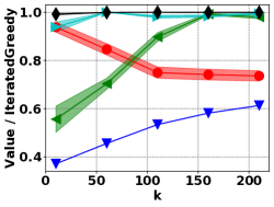
(a) Objective, small $k$

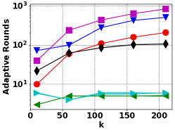
(b) Rounds, small $k$

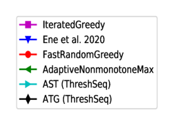
(c) Legend

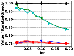
(d) Objective, large $k$

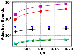
(e) Rounds, large $k$

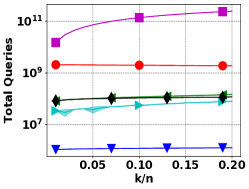
(f) Queries, large $k$

Figure 1: Comparison of objective value (normalized by the IteratedGreedy objective value), total queries, and adaptive rounds on web-Google for the maxcut application for both small and large $k$ values. The large $k$ values are given as a fraction of the number of nodes in the network. The algorithm of ?’s (?) is run with oracle access to the multilinear extension and its gradient; total queries reported for this algorithm are queries to these oracles, rather than the original set function.

Results on cardinality-constrained maximum cut. In Fig. 1, we show representative results for cardinality-constrained maximum cut on web-Google ($n=875713$) for both small and large $k$ values. Results on other datasets and revenue maximization are given in Appendix G. In addition, results for ?’s (?) when the multilinear extension is approximated via sampling are given in Appendix G. The algorithms are evaluated by objective value of solution, total queries made to the oracle, and the number of adaptive rounds (lower is better). Objective value is normalized by that of IteratedGreedy.

In terms of objective value (Figs. 1(a) and 1(d)), our algorithm ATG maintained better than $0.99$ of the IteratedGreedy value, while all other algorithms fell below $0.95$ of the IteratedGreedy value on some instances. Our algorithm AST obtained similar objective value to AdaptiveNonmonotoneMax on larger $k$ values, but performed much better on small $k$ values. Finally, the algorithm of ?’s (?) obtained poor objective value for $k\leq 100$ and about $0.75$ of the IteratedGreedy value on larger $k$ values. It is interesting to observe that the two algorithms with the best approximation ratio of $1/e$, ?’s (?) and FastRandomGreedy, returned the worst objective values on larger $k$ (Fig. 1(d)).

For total queries (Fig. 1(f)), the most efficient is ?’s (?), although it does not query the set function directly, but the multilinear extension and its gradient. The most efficient of the combinatorial algorithms was AST, followed by ATG. Finally, with respect to the number of adaptive rounds (Fig. 1(e)), the best was AdaptiveNonmonotoneMax, closely followed by AST; the next lowest was ATG, followed by ?’s (?).

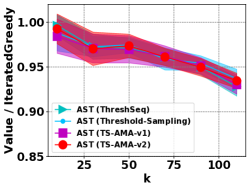
(a) Objective, BA

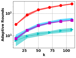
(b) Rounds, BA

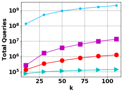
(c) Queries, ca-GrQc

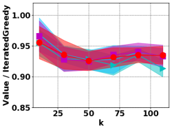
(d) Objective, ca-GrQc

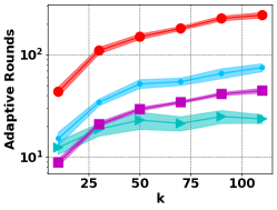
(e) Rounds, ca-GrQc

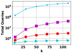
(f) Queries, ca-GrQc

Figure 2: Results of AST with four threshold sampling procedures on two datasets. The algorithms are run strictly following pseudocode.

Comparison of different threshold sampling procedures. Fig. 2 shows the results of AST with different threshold sampling procedures for cardinality-constrained maximum cut on two datasets, BA ($n=968$) and ca-GrQc ($n=5242$). All the algorithms are run according to pseudocode without any modification. TS-AMA-v1 and TS-AMA-v2 represent the ThreshSeq algorithms without and with binary search proposed in ?’s (?).

For objective values, all four versions of AST return similar results; see Figs. 2(a) and 2(d). As for adaptive rounds, ThreshSeq, Threshold-Sampling, and TS-AMA-v1 all run in $O\left(\log(n)\right)$ rounds, while TS-AMA-v2 runs in $O\left(\log^{2}(n)\right)$ rounds. By the results in Figs. 2(b) and 2(e), our ThreshSeq is the most highly parallelizable algorithm, followed by TS-AMA-v1. TS-AMA-v2 is significantly worst as what it is in theory. With respect to the query calls, while our ThreshSeq only queries once for each prefix, Threshold-Sampling queries $16\lceil\log(2/\hat{\delta})/\hat{\varepsilon}^{2}\rceil$ times, and both TS-AMA-v1 and TS-AMA-v2 query $|V|$ times. According to Figs. 2(c) and 2(f), our ThreshSeq is the most query efficient one among all. Also, the total queries do not increase a lot when $k$ increases. With binary search, TS-AMA-v2 is the second best one which has $O\left(n\log^{2}(n)\right)$ query complexity. As for Threshold-Sampling, with the input values as $n=968$, $k=10$, and $\varepsilon=\delta=0.1$, it queries about $2\times 10^{5}$ times for each prefix which is significantly large.

Among all, ThreshSeq proposed in this paper is not only the best theoretically, but also performs well in experiments compared with the pre-existing threshold sampling algorithms.

A Probability Lemma and Concentration Bounds

Lemma 12.

(Chernoff bounds (?)). Suppose $X_{1}$, … , $X_{n}$ are independent binary random variables such that $Pr\left(X_{i}=1\right)=p_{i}$. Let $\mu=\sum_{i=1}^{n}p_{i}$, and $X=\sum_{i=1}^{n}X_{i}$. Then for any $\delta\geq 0$, we have

$$Pr\left(X\geq(1+\delta)\mu\right)\leq e^{-\frac{\delta^{2}\mu}{2+\delta}}.$$ (8)

Moreover, for any $0\leq\delta\leq 1$, we have

$$Pr\left(X\leq(1-\delta)\mu\right)\leq e^{-\frac{\delta^{2}\mu}{2}}.$$ (9)

Lemma 13.

(?). Suppose there is a sequence of $n$ Bernoulli trials: $X_{1},X_{2},\ldots,X_{n},$ where the success probability of $X_{i}$ depends on the results of the preceding trials $X_{1},\ldots,X_{i-1}$. Suppose it holds that

$$Pr\left(X_{i}=1|X_{1}=x_{1},X_{2}=x_{2},\ldots,X_{i-1}=x_{i-1}\right)\geq\eta,$$

where $\eta>0$ is a constant and $x_{1},\ldots,x_{i-1}$ are arbitrary.

Then, if $Y_{1},\ldots,Y_{n}$ are independent Bernoulli trials, each with probability $\eta$ of success, then

$$Pr\left(\sum_{i=1}^{n}X_{i}\leq b\right)\leq Pr\left(\sum_{i=1}^{n}Y_{i}\leq b\right),$$

where $b$ is an arbitrary integer.

Moreover, let $A$ be the first occurrence of success in sequence $X_{i}$. Then,

$$\mathbb{E}\left[A\right]\leq 1/\eta.$$

Lemma 14.

(?). Suppose there is a sequence of $n+1$ Bernoulli trials: $X_{1},X_{2},\ldots,X_{n+1},$ where the success probability of $X_{i}$ depends on the results of the preceding trials $X_{1},\ldots,X_{i-1}$, and it decreases from 1 to 0. Let $t$ be a random variable based on the $n+1$ Bernoulli trials. Suppose it holds that

$$Pr\left(X_{i}=1|X_{1}=x_{1},X_{2}=x_{2},\ldots,X_{i-1}=x_{i-1},i\leq t\right)\geq\eta,$$

where $x_{1},\ldots,x_{i-1}$ are arbitrary and $0<\eta<1$ is a constant. Then, if $Y_{1},\ldots,Y_{n+1}$ are independent Bernoulli trials, each with probability $\eta$ of success, then

$$Pr\left(\sum_{i=1}^{t}X_{i}\leq bt\right)\leq Pr\left(\sum_{i=1}^{t}Y_{i}\leq bt\right),$$

where $b$ is an arbitrary integer.

B Counterexample for Threshold-Sampling with Non-monotone Submodular Functions

?’s (?) proposed a subroutine, Threshold-Sampling, which returns a solution $S\subseteq\mathcal{N}$ that $\mathbb{E}\left[f(S)/S\right]\geq(1-\varepsilon)\tau$ within logarithmic rounds and linear time. The full pseudocode for Threshold-Sampling is given in Alg. 5. The notation $\mathcal{U}(S,t)$ represents the uniform distribution over subsets of $S$ of size $t$. Threshold-Sampling relies upon the procedure ReducedMean, given in Alg. 4. The Bernoulli distribution input to ReducedMean is the distribution $\mathcal{D}_{t}$, which is defined as follows.

Definition 15.

Conditioned on the current state of the algorithm, consider the process where the set $T\sim\mathcal{U}(A,t-1)$ and then the element $x\sim A\setminus T$ are drawn uniformly at random. Let $\mathcal{D}_{t}$ denote the probability distribution over the indicator random variable

$$I_{t}=\mathbb{I}[f(S\cup T+x)-f(S\cup T)\geq\tau].$$

Below, we state the lemma of Threshold-Sampling in ?’s (?).

Lemma 16 (?’s (?)).

The algorithm Threshold-Sampling outputs $S\subseteq\mathcal{N}$ with $|S|\leq k$ in $O(\log(n/\delta)/\varepsilon)$ adaptive rounds such that the following properties hold with probability at least $1-\delta$:

• There are $O(n/\varepsilon)$ oracle queries in expectation.

• The expected average marginal $\mathbb{E}\left[f(S)/|S|\right]\geq(1-\varepsilon)\tau$.

• If $|S|<k$, then $f_{x}(S)<\tau$ for all $x\in\mathcal{N}$.

In ?’s (?) and ?’s (?), the above Lemma is used with non-monotone submodular functions; however, in the case that $f$ is non-monotone, the lemma does not hold. Alg. 4 only checks (on Line 13) if there is more than a constant fraction of elements whose marginal gains are larger than the threshold $\tau$. If there exist elements with large magnitude, negative marginal gains, then the average marginal gain may fail to satisfy the lower bound in Lemma 16. As for the proof in ?’s (?), the following inequality does not hold (needed for the proof of Lemma 3.3 of ?’s (?)):

$$\mathbb{E}\left[\Delta\left(T\,|\,S\right)\right]\geq(\mathbb{E}\left[I_{1}\right]+\mathbb{E}\left[I_{2}\right]+\ldots+\mathbb{E}\left[I_{t}\right])\tau,$$

where $|T|=t^{*}$ and $t\geq t^{*}/(1+\hat{\varepsilon})$. Next, we give a counterexample for the two versions of Threshold-Sampling used in ?’s (?) and ?’s (?) where the only difference is that the if condition in Alg. 5 on Line 9 changes to $|A|<3k$ in ?’s (?).

Algorithm 4 The ReducedMean algorithm of ?’s (?)

1:Input: access to a Bernoulli distribution $\mathcal{D}$, error $\varepsilon$, failure probability $\delta$

2:Set number of samples $m\leftarrow 16\lceil\log(2/\delta)/\varepsilon^{2}\rceil$

3:Sample $X_{1},X_{2},\ldots,X_{m}\sim\mathcal{D}$

4:Set $\bar{\mu}\leftarrow\frac{1}{m}\sum_{i=1}^{m}X_{i}$

5:if  $\bar{\mu}\leq 1-1.5\varepsilon$  then

6:     return true

7:return false

Algorithm 5 The threshold sampling algorithm of ?’s (?)

1:procedure Threshold-Sampling($f,k,\tau,\varepsilon,\delta$)

2:     Input: evaluation oracle $f:2^{\mathcal{N}}\to\mathbb{R}^{+}$, constraint $k$, threshold $\tau$, error $\varepsilon$, failure probability $\delta$

3:     Set smaller error $\hat{\varepsilon}\leftarrow\varepsilon/3$

4:     Set iteration bounds $r\leftarrow\lceil\log_{(1-\hat{\varepsilon})^{-1}}(2n/\delta)\rceil,m\leftarrow\lceil\log(k)/\hat{\varepsilon}\rceil$

5:     Set smaller failure probability $\hat{\delta}\leftarrow\delta/(2r(m+1))$

6:     Initialize $S\leftarrow\emptyset,A\leftarrow N$

7:     for  $r$ sequential rounds  do

8:         Filter $A\leftarrow\{x\in A:\Delta(x,S)\geq\tau\}$

9:         if $|A|=0$ then

10:              break          

11:         for $i=0$ to $m$ in parallel do

12:              Set $t\leftarrow\min\{\lfloor(1+\hat{\varepsilon})^{i}\rfloor,|A|\}$

13:              $rm[t]\leftarrow$ReducedMean $(\mathcal{D}_{t},\hat{\varepsilon},\hat{\delta})$          

14:         $t^{\prime}\leftarrow\min t$ such that $rm[t]$ is true

15:         Sample $T\sim\mathcal{U}\left(A,\min\{t^{\prime},k-|S|\}\right)$

16:         Update $S\leftarrow S\cup T$

17:         if  $|S|=k$  then

18:              break               

19:     return $S$

Counterexample 1. Define a set function $f:2^{\mathcal{N}}\to\mathbb{R}^{+}$ as follows,

$$f(B)=\left\{\begin{aligned} &n^{2}+|B|,&\text{if }a\not\in B\\ &n^{2}+1-(|B|-1)n,&\text{if }a\in B\end{aligned}\right..$$

Let $k=n=|\mathcal{N}|>400$, $\tau=1$, $\varepsilon=0.1$, $\delta=0.1$. Run $\textsc{Threshold-Sampling}(f,k,\tau,\varepsilon,\delta)$.

Proof.

For any $B\subseteq\mathcal{N}$ and $x\in\mathcal{N}\backslash B$, the above set function follows that

$$\Delta\left(x\,|\,B\right)=\left\{\begin{aligned} &1,&&\text{if }x\neq a\text{ and }a\not\in B\\ &-n,&&\text{if }x\neq a\text{ and }a\in B\\ &1-|B|(n+1),&&\text{if }x=a\end{aligned}\right..$$

Thus, $f$ is a non-negative, non-monotone submodular function. For any $1<t\leq|\mathcal{N}|$, $|T|=t-1$, and $S=\emptyset$,

$$\mathbb{E}\left[I_{t}\right]=Pr\left(f(S\cup T+x)-f(S\cup T)\geq\tau\right)=Pr\left(x\neq a\text{ and }a\not\in T\right)=1-\frac{t}{n}.$$

So, with any value of $\varepsilon$, ReducedMean returns true when $t>\varepsilon n/2$. The first round of Threshold-Sampling samples a set $T_{1}$ with $t_{1}^{\prime}=|T_{1}|>\varepsilon n/2$. Then update $S$ by $S=T_{1}$.

For the Threshold-Sampling in ?’s (?) with stop condition $|A|<3k$, the algorithm stopped here after the first iteration, no matter what is sampled. In this case, the expectation of marginal gains of the set returned by the algorithm would be as follows,

$$\mathbb{E}\left[\Delta\left(S\,|\,\emptyset\right)\right] =Pr\left(a\in T_{1}\right)\Delta\left(T_{1}\,|\,\emptyset\right)+Pr\left(a\not\in T_{1}\right)\Delta\left(T_{1}\,|\,\emptyset\right)$$

$$=\frac{t_{1}^{\prime}}{n}\left(1-(t_{1}^{\prime}-1)n\right)+\frac{n-t_{1}^{\prime}}{n}t_{1}^{\prime}$$

$$=t_{1}^{\prime}\left(2-t_{1}^{\prime}+\frac{1-t_{1}^{\prime}}{n}\right)<0.$$

Next, we consider the Threshold-Sampling with stop condition $|A|=0$. After the first iteration discussed above, if $a\in T_{1}$, all the elements would be filtered out at the second round. Algorithm stoped here and returned $S$, say $S_{1}$. If $a\not\in T_{1}$, $T_{1}$ and $a$ would be filtered out at the second round, which means $A=\mathcal{N}\backslash(S\cup\{a\})$. And for any $T\subseteq A$ and $x\in A\backslash T$,

$$f(S\cup T+x)-f(S\cup T)=1.$$

Therefore, $\mathbb{E}\left[I_{t}\right]=1$ for all $t$. After several iterations, $S=\mathcal{N}\backslash\{a\}$ would be returned, say $S_{2}$.

The expectation of objective value of the set returned would be as follows,

$$\mathbb{E}\left[\Delta\left(S\,|\,\emptyset\right)\right] =Pr\left(a\in T_{1}\right)\Delta\left(S_{1}\,|\,\emptyset\right)+Pr\left(a\not\in T_{1}\right)\Delta\left(S_{2}\,|\,\emptyset\right)$$

$$=\frac{t_{1}^{\prime}}{n}(1-(t_{1}^{\prime}-1)n)+\frac{n-t_{1}^{\prime}}{n}(n-1)$$

$$=\frac{2t_{1}^{\prime}}{n}-1-t_{1}^{\prime 2}+n<0,$$

since $\varepsilon=0.1$, $n>400$, and $\varepsilon n/2<t_{1}^{\prime}<\varepsilon(1+\varepsilon/3)n/2$.

∎

C Analysis of ThreshSeq

See 4

proof of Lemma 4.

After filtering on Line 5, any element $x\in V$ follows that $\Delta\left(x\,|\,A\right)\geq\tau$. Therefore, $S_{0}=\emptyset$. Also, it is obvious that $\Delta\left(x\,|\,A\cup V\right)=0$. So, $S_{|V|}=V$. Next, let’s consider any $x\in S_{i-1}$. By submodularity,

$$\Delta\left(x\,|\,A\cup T_{i}\right)\leq\Delta\left(x\,|\,A\cup T_{i-1}\right)<\tau.$$

Thus, for any $x\in S_{i-1}$, it holds that $x\in S_{i}$, which means $S_{i-1}\subseteq S_{i}$. ∎

See 5

proof of Lemma 5.

Call an element $v_{i}\in V$ bad iff $\Delta\left(v_{i}\,|\,A\cup T_{i-1}\right)<\tau$; and good, otherwise. The random permutation of $V$ can be regarded as $|V|$ dependent Bernoulli trials, with success iff the element is bad and failure otherwise. Observe that, the probability that an element in $T_{i}$ is bad, when $i\leq t$, is less than $\varepsilon/2$, conditioned on the outcomes of the preceding trials. We know that,

$$Pr\left(i^{*}<\min\{s,t\}\right)\leq Pr\left(\#\text{ bad elements in }T_{i^{\prime}}>\varepsilon i^{\prime}\text{, where }i^{\prime}=\min\{s,t\}\right).$$

Let $X_{i}=1$, if $v_{i}$ is bad; and $X_{i}=0$, otherwise. Then, $(X_{i})$ is a sequence of dependent Bernoulli trails. And for any $i\leq i^{\prime}$, $Pr\left(X_{i}=1\right)\leq\varepsilon/2$. Let $(Y_{i})$ be a sequence of independent and identically distributed Bernoulli trails, each with success probability $\varepsilon/2$. Then, the probability of $i^{*}<\min\{s,t\}$ can be bounded as follows:

$$Pr\left(i^{*}<\min\{s,t\}\right)\leq Pr\left(\sum_{i=1}^{i^{\prime}}X_{i}>\varepsilon i^{\prime}\right)\overset{(a)}{\leq}Pr\left(\sum_{i=1}^{i^{\prime}}Y_{i}>\varepsilon i^{\prime}\right)\overset{(b)}{\leq}1/2,$$

where Inequality (a) follows from Lemma 14, and Inequality (b) follows from Law of Total Probability and Markov’s inequality. ∎

proof of success probability.

When the algorithm fails to terminate, at each iteration, it always holds that $i^{*}<s$; and there are no more than $m=\lceil\log_{1-\varepsilon/2}(1/n)\rceil$ iterations that $i^{*}\geq t$. Therefore, there are no more than $m$ iterations that $i^{*}\geq\min\{s,t\}$. Otherwise, with more than $m$ iterations that $i^{*}\geq\min\{s,t\}$, if there is an iteration that $s\leq t$, the algorithm terminates with $|A|=k$. Otherwise, with more than $m$ iterations that $i^{*}\geq t$, the algorithm terminates with $|V|=0$. Define a successful iteration as an iteration that $i^{*}\geq\min\{s,t\}$, which means it successfully filters out $\varepsilon/2$-fraction of $V$ or the algorithm stops here. Let $X$ be the number of successes in the $\ell$ iterations. Then, $X$ can be regarded as a sum of dependent Bernoulli trails, where the success probability is larger than 1/2 from Lemma 5. Let $Y$ be a sum of independent Bernoulli trials, where the success probability is equal to 1/2. Then, the probability of failure can be bounded as follows,

$$Pr\left(\text{failure}\right) \leq Pr\left(X\leq m\right)$$

$$\overset{(a)}{\leq}Pr\left(Y\leq m\right)$$

$$\leq Pr\left(Y\leq 2\log(n)/\varepsilon\right)$$

$$\overset{(b)}{\leq}e^{-\left(\frac{\log(n)}{2\log(n)+\varepsilon\log\left(\frac{n}{\delta}\right)}-1\right)^{2}\cdot\left(\frac{2}{\varepsilon}\log(n)+\log\left(\frac{n}{\delta}\right)\right)}$$

$$=e^{-\log\left(\frac{n}{\delta}\right)-\frac{\log^{2}(n)}{\varepsilon^{2}\log\left(\frac{n}{\delta}\right)+2\varepsilon\log(n)}}$$

$$\leq\frac{\delta}{n},$$

where Inequality (a) follows from Lemma 13, and Inequality (b) follows from Lemma 12. ∎

See 6

proof of Lemma 6.

Let $A_{j}$ be the set $A$ after iteration $j$, $T_{j,i}$ be the first $i$ elements of $V_{j}$ at $j$-th iteration. Similarly, define $A_{j}^{\prime}$ as the set $A^{\prime}$ after iteration $j$, $T^{\prime}_{j,i}=T_{j,i}[\text{where }B[1:i]\not=\textbf{false}]$.

From Algorithm 1, $A=\sum_{j=1}^{\ell}T_{j,i^{*}}$. For each $T_{j,i^{*}}$, there are at least $(1-\varepsilon)$-fraction of $T_{j,i^{*}}$ are good. Totally, there are at least $(1-\varepsilon)$-fraction of $A$ are good.

By Line 17, $T^{\prime}_{j,i}$ only contains the elements with nonnegative marginal gains in $T_{j,i}$. Therefore, any element in $A^{\prime}$ has nonnegative marginal gain when added. For any good element $v_{i}\in V_{j}$, by submodularity, $\Delta\left(v_{i}\,|\,A^{\prime}_{j-1}\cup T^{\prime}_{j,i-1}\right)\geq\Delta\left(v_{i}\,|\,A_{j-1}\cup T_{j,i-1}\right)\geq\tau$. Thus, a good element in $A$ is always good in $A^{\prime}$. ∎

Calculation of Query Complexity.

Let $V_{j}$ be the set $V$ after filtering on Line 5 at iteration $j$, $j_{i}$ be the iteration which is the $i$-th successful iterations, $Y_{i}=j_{i}-j_{i-1}$. By Lemma 13, it holds that $\mathbb{E}\left[Y_{i}\right]\leq 2$. For any iteration $j$ that $j_{i-1}+1\leq j\leq j_{i}$, there are $i-1$ successes before it. Thus, it holds that $|V_{j}|\leq n(1-\varepsilon/2)^{i-1}$.

At any iteration $j$, there are $|V_{j-1}|+1$ oracle queries on Line 5. As for the inner for loop, there are no more than $|V_{j}|+1$ oracle queries. The expected number of total queries can be bounded as follows:

$$\mathbb{E}\left[\text{Queries}\right] \leq\sum_{j=1}^{\ell}\mathbb{E}\left[|V_{j-1}|+|V_{j}|+2\right]$$

$$\leq n+2\ell+\sum_{j=1}^{\ell}2\mathbb{E}\left[|V_{j}|\right]$$

$$\leq n+2\ell+\sum_{i\geq 1}2\mathbb{E}\left[Y_{i}\cdot n(1-\varepsilon/2)^{i-1}\right]$$

$$\leq n+2\ell+4n/\varepsilon.$$

Therefore, the total queries are $O\left(n/\varepsilon\right)$. ∎

D ThresholdGreedy and Modification

Algorithm 6 The ThresholdGreedy Algorithm of ?’s (?)

1:procedure ThresholdGreedy($f,k,\varepsilon$)

2:     Input: evaluation oracle $f:2^{\mathcal{N}}\to\mathbb{R}^{+}$, constraint $k$, accuracy parameter $\varepsilon>0$

3:     $M\leftarrow\arg\,\max_{x\in\mathcal{N}}f(x)$;

4:     $S\leftarrow\emptyset$

5:     for  $\tau=M$; $\tau\geq(1-\varepsilon)M/k$; $\tau\leftarrow\tau(1-\varepsilon)$ do

6:         for  $x\in\mathcal{N}$  do

7:              if  $f(S+x)-f(S)\geq\tau$  then

8:                  $S\leftarrow S+x$

9:                  if  $|S|=k$  then

10:                       break from outer for                                               

11:     return $S$

In this section, we describe ThresholdGreedy (Alg. 6) of ?’s (?) and how it is modified to have low adaptivity. This algorithm achieves ratio $1-1/e-\varepsilon$ in $O(n\log k)$ queries if the function $f$ is monotone but has no constant ratio if $f$ is not monotone.

The ThresholdGreedy algorithm works as follows: a set $S$ is initialized to the empty set. Elements whose marginal gain exceed a threshold value are added to the set in the following way: initially, a threshold of $\tau=M=\arg\,\max_{a\in\mathcal{N}}f(a)$ is chosen, which is iteratively decreased by a factor of $(1-\varepsilon)$ until $\tau<M/k$. For each threshold $\tau$, a pass through all elements of $\mathcal{N}$ is made, during which any element $x$ that satisfies $f(S+x)-f(S)\geq\tau$ is added to the set $S$. While this strategy leads to an efficient $O(n\log k)$ total number of queries, it also has $\Omega(n\log k)$ adaptivity, as each query depends on the previous ones.

To make this approach less adaptive, we replace the highly adaptive pass through $\mathcal{N}$ (the inner for loop) with a single call to Threshold-Sampling, which requires $O(\log n)$ adaptive rounds and $O(n/\varepsilon)$ queries in expectation. This modified greedy approach appears twice in ATG (Alg. 3), corresponding to the two for loops.

E Improved Ratio for IteratedGreedy

Algorithm 7 The IteratedGreedy Algorithm of ?’s (?)

1:procedure IteratedGreedy($f,k$)

2:     Input: evaluation oracle $f:2^{\mathcal{N}}\to\mathbb{R}^{+}$, constraint $k$,

3:     $A\leftarrow\emptyset$

4:     for  $i\leftarrow 1$ to $k$  do

5:         $a_{i}\leftarrow\arg\,\max_{x\in\mathcal{N}}f(A+x)-f(A)$

6:         $A\leftarrow A+a_{i}$      

7:     $B\leftarrow\emptyset$

8:     for  $i\leftarrow 1$ to $k$  do

9:         $b_{i}\leftarrow\arg\,\max_{x\in\mathcal{N}\setminus A}f(B+x)-f(B)$

10:         $B\leftarrow B+b_{i}$      

11:     $A^{\prime}\leftarrow$ UnconstrainedMax $(A)$

12:     return $C\leftarrow\arg\,\max\{f(A),f(A^{\prime}),f(B)\}$

In this section, we prove an improved approximation ratio for the algorithm IteratedGreedy of ?’s (?), wherein a ratio of $1/(4+\alpha)$ is proven given access to a $1/\alpha$-approximation for UnconstrainedMax. We improve this ratio to $\frac{e-1}{e(2+\alpha)-\alpha}\approx 0.193$ if $\alpha=2$. Pseudocode for IteratedGreedy is given in Alg. 7.

IteratedGreedy works as follows. First a standard greedy procedure is run which produces set $A$ of size $k$. Next, a second greedy procedure is run to yield set $B$; during this second procedure, elements of $A$ are ignored. A subroutine for UnconstrainedMax is used on $f$ restricted to $A$, which yields set $A^{\prime}$. Finally the set of $\{A,A^{\prime},B\}$ that maximizes $f$ is returned.

Theorem 17.

Suppose there exists an $(1/\alpha)$-approximation for UnconstrainedMax. Then by using this procedure as a subroutine, the algorithm IteratedGreedy has approximation ratio $\frac{e-1}{e(2+\alpha)-\alpha}$ for SMCC.

Proof.

For $1\leq i\leq k$, let $a_{i},b_{i}$ be as chosen during the run of IteratedGreedy. Define $A_{i}=\{a_{1},\ldots,a_{i-1}\}$, $B_{i}=\{b_{1},\ldots,b_{i-1}\}$. Then for for any $1\leq i\leq k$, we have

$$f(A_{i+1})+f(B_{i+1})-f(A_{i})-f(B_{i}) =f_{a_{i}}(A_{i})+f_{b_{i}}(B_{i})$$

$$\geq\frac{1}{k}\sum_{o\in O}f_{o}(A_{i})+\frac{1}{k}\sum_{o\in O\setminus A}f_{o}(B_{i})$$

$$\geq\frac{1}{k}\left(f\left(O\cup A_{i}\right)-f\left(A_{i}\right)+f\left((O\setminus A)\cup B_{i}\right)-f\left(B_{i}\right)\right)$$

$$\geq\frac{1}{k}\left(f\left(O\setminus A\right)-(f\left(A_{i}\right)+f\left(B_{i}\right))\right),$$

where the first inequality follows from the greedy choices, the second follows from submodularity, and the third follows from submodularity and the fact that $A_{i}\cap B_{i}=\emptyset$. Hence, from this recurrence and standard arguments,

$$f(A)+f(B)\geq(1-1/e)f\left(O\setminus A\right),$$

where $A,B$ have their values at termination of IteratedGreedy. Since $f(A^{\prime})\geq f(O\cap A)/\alpha$, we have from submodularity

$$f(O) \leq f(O\cap A)+f(O\setminus A)$$

$$\leq\alpha f(A^{\prime})+(1-1/e)^{-1}(f(A)+f(B))$$

$$\leq(\alpha+2(1-1/e)^{-1})f(C).$$

∎

F Proofs for Section 4

In this section, we provide the proofs omitted from Section 4.

See 9

proof of Lemma 9.

Since each element in $A^{\prime}$ has nonnegative marginal gain, it always holds that $f(\mathcal{A}_{j}^{\prime})\geq f(\mathcal{A}_{j-1}^{\prime})$.

From Lemma 6, there are at least $(1-\varepsilon)$-fraction of $A$ are good elements. Therefore, there are at least $(1-\varepsilon)k$ of $a_{j}^{\prime}$ which is good element or dummy element. Next, let’s consider the following 3 cases of $a_{j}^{\prime}$.

Case $i(j)=1$ and $a_{j}^{\prime}$ is good. By Theorem 3 and Lemma 6, it holds that

$$f(\mathcal{A}_{j}^{\prime})-f(\mathcal{A}_{j-1}^{\prime})\geq\tau_{1}=M\geq\frac{1}{k}\sum_{o\in O}f(o)\geq\frac{1}{k}f(O).$$

Case $i(j)>1$ and $a_{j}^{\prime}$ is good. Since $a_{j}^{\prime}$ is returned at iteration $i(j)$ and $a_{j}^{\prime}$ is good, it holds that: (1) $f(\mathcal{A}_{j}^{\prime})-f(\mathcal{A}_{j-1}^{\prime})\geq\tau_{i(j)}$; (2) at previous iteration $i(j)-1$, ThreshSeq returns $S_{i(j)-1}$ that $|S_{i(j)-1}|<k-|A_{i(j)-2}|$. By property (2) and Theorem 3, for any $o\in O\backslash A_{i(j)-1}$, $\Delta\left(o\,|\,A_{i(j)-1}\right)<\tau_{i(j)-1}$. Then,

$$f(\mathcal{A}_{j}^{\prime})-f(\mathcal{A}_{j-1}^{\prime}) \geq\tau_{i(j)}=(1-\varepsilon^{\prime})\tau_{i(j)-1}$$

$$>\frac{1-\varepsilon^{\prime}}{k}\sum_{o\in O\backslash A_{i(j)-1}}\Delta\left(o\,|\,A_{i(j)-1}\right)$$

$$\geq\frac{1-\varepsilon^{\prime}}{k}\left(f(O\cup A_{i(j)-1})-f(A_{i(j)-1})\right)$$

$$\geq\frac{1-\varepsilon^{\prime}}{k}\left(f(O\cup A_{i(j)-1})-f(A^{\prime}_{i(j)-1})\right)$$ (10)

$$\geq\frac{1-\varepsilon^{\prime}}{k}\left(f(O\cup A_{i(j)-1})-f(\mathcal{A}_{j-1}^{\prime})\right),$$ (11)

where Inequality 10 follows from the proof of Lemma 6, and Inequality 11 follows from $A^{\prime}_{i(j)-1}\subseteq\mathcal{A}_{j-1}^{\prime}$.

Case $i(j)=\ell+1$ (or $a_{j}^{\prime}$ is dummy element). In this case, $|A|<k$ when the first for loop ends. So, ThreshSeq in the last iteration returns $S_{\ell}$ that $|S_{\ell}|<k-|A_{\ell-1}|$. From Theorem 3, it holds that $\Delta\left(o\,|\,A_{\ell}\right)<\tau_{\ell}<\frac{M}{ck}$, for any $o\in O\backslash A_{\ell}$. Thus,

$$\frac{M}{ck}>\frac{1}{k}\sum_{o\in O\backslash A_{\ell}}\Delta\left(o\,|\,A_{\ell}\right)\geq\frac{1}{k}\left(f(O\cup A_{\ell})-f(A_{\ell})\right)\overset{(a)}{\geq}\frac{1}{k}\left(f(O\cup A_{\ell})-f(\mathcal{A}_{j}^{\prime})\right),$$

where Inequality (a) follows from $A_{\ell}=A$ and $f(\mathcal{A}_{j}^{\prime})=f(A^{\prime})$.

The first inequality of Lemma 9 holds in those three cases with at least $(1-\varepsilon^{\prime})k$ of $j$. ∎

See 11

Proof of Lemma 11.

From Lemma 9, $f(\mathcal{A^{\prime}}_{j(u)-1})\geq f(\mathcal{A^{\prime}}_{j(u-1)})$, and

$$f(\mathcal{A}_{j(u)}^{\prime}) \geq\left(1-\frac{1-\varepsilon^{\prime}}{k}\right)f(\mathcal{A}_{j(u)-1}^{\prime})+\frac{1-\varepsilon^{\prime}}{k}f(O\cup A_{i(j(u))-1})-\frac{M}{ck}$$

$$\geq\left(1-\frac{1-\varepsilon^{\prime}}{k}\right)f(\mathcal{A}_{j(u-1)}^{\prime})+\frac{1-\varepsilon^{\prime}}{k}f(O\cup A_{i(j(u))-1})-\frac{M}{ck}.$$

Similarly,

$$f(\mathcal{B}_{j(u)}^{\prime})\geq\left(1-\frac{1-\varepsilon^{\prime}}{k}\right)f(\mathcal{B}_{j(u-1)}^{\prime})+\frac{1-\varepsilon^{\prime}}{k}f((O\backslash A)\cup B_{i(j(u))-1})-\frac{M}{ck}.$$

By adding the above two inequalities and the submodularity, we have,

$$\Gamma_{u} \geq\left(1-\frac{1-\varepsilon^{\prime}}{k}\right)\Gamma_{u-1}+\frac{1-\varepsilon^{\prime}}{k}\left(f(O\cup A_{i(j(u))-1})+f((O\backslash A)\cup B_{i(j(u))-1})\right)-\frac{2M}{ck}$$

$$\geq\left(1-\frac{1-\varepsilon^{\prime}}{k}\right)\Gamma_{u-1}+\frac{1-\varepsilon^{\prime}}{k}f(O\backslash A)-\frac{2M}{ck}.$$

∎

Lemma 18.

Let $\varepsilon\in(0,1)$, and suppose $c=8/\varepsilon$, $\varepsilon^{\prime}=(1-1/e)\varepsilon/8$, and $\beta=1-e^{(1-\varepsilon^{\prime})^{2}}$. Then

$$\left(\frac{1-\frac{2}{c(1-\varepsilon^{\prime})^{2}}}{\alpha+\frac{2}{\beta}}\right)\geq\left(\frac{e-1}{\alpha(e-1)+2e}-\varepsilon\right).$$ (12)

Proof of Lemma 18.

We start with the following two inequalities, which are verified below.

$$1-\frac{2}{c(1-\varepsilon^{\prime})^{2}}\geq 1-\varepsilon$$ , (13)

$$\frac{2}{1-e^{-(1-\varepsilon^{\prime})^{2}}}\leq\frac{2}{1-1/e}+\varepsilon/2$$ . (14)

Let $A=1$, $B=1/\alpha+2/(1-1/e)$. From the inequalities above, the left-hand side of (12) is at least $\frac{A-\varepsilon}{B+\varepsilon}$ and

$$\frac{A-\varepsilon}{B+\varepsilon}\geq\frac{A}{B}-\varepsilon \iff\varepsilon\geq\frac{A}{B}-\frac{A-\varepsilon}{B+\varepsilon}$$

$$\iff 1\geq\frac{A}{\varepsilon B}-\frac{A}{\varepsilon(B+\varepsilon)}+\frac{1}{B+\varepsilon}.$$

Next,

$$\frac{A}{\varepsilon B}-\frac{A}{\varepsilon(B+\varepsilon)}+\frac{1}{B+\varepsilon}=\frac{A}{B(B+\varepsilon)}+\frac{1}{B+\varepsilon}\leq 1/4+1/2<1,$$

since $B\geq 2$ and $A=1$. Finally, $A/B=\frac{\alpha(e-1)}{e-1+2\alpha e}$.

Proof of (13).

$$c\geq 8/\varepsilon=\frac{2}{\varepsilon(1/2)^{2}}\geq\frac{2}{\varepsilon(1-\varepsilon^{\prime})^{2}},$$

since $\varepsilon^{\prime}=(1-1/e)\varepsilon/8\leq 1/2$.

Proof of (14). Let $\lambda=1-1/e$, $\kappa=e^{-(1-\varepsilon^{\prime})^{2}}$. Inequality (14) is satisfied iff.

$$2\lambda\leq 2(1-\kappa)+\frac{\lambda\varepsilon(1-\kappa)}{2} \iff 2\lambda\leq 2-2\kappa+\lambda\varepsilon/2-\lambda\varepsilon\kappa/2$$

$$\iff 2\kappa+\lambda\varepsilon\kappa/2\leq\lambda\varepsilon/2+2-2\lambda$$

$$\iff\kappa=e^{-(1-\varepsilon^{\prime})^{2}}\leq\frac{\lambda\varepsilon/2+2-2\lambda}{2+\lambda\varepsilon/2}$$

$$\iff(1-\varepsilon^{\prime})^{2}\geq\log\left(\frac{2+\lambda\varepsilon/2}{\lambda\varepsilon/2+2-2\lambda}\right),$$

which in turn is satisfied if

$$2\varepsilon^{\prime}\leq 1-\log\left(\frac{2+\lambda\varepsilon/2}{\lambda\varepsilon/2+2-2\lambda}\right).$$

Then

$$2\varepsilon^{\prime}=\lambda\varepsilon/4\leq\frac{2+\lambda\varepsilon/2-4\lambda}{2-\lambda} \leq\frac{2+\lambda\varepsilon/2-4\lambda}{2+\lambda\varepsilon/2-2\lambda}$$

$$=\frac{2(\lambda\varepsilon/2+2-2\lambda)-2-\lambda\varepsilon/2}{\lambda\varepsilon/2+2-2\lambda}$$

$$=2-\frac{2+\lambda\varepsilon/2}{\lambda\varepsilon/2+2-2\lambda}$$

$$=1-\left(\frac{2+\lambda\varepsilon/2}{\lambda\varepsilon/2+2-2\lambda}-1\right)$$

$$\leq 1-\log\left(\frac{2+\lambda\varepsilon/2}{\lambda\varepsilon/2+2-2\lambda}\right),$$

where we have used $\log x\leq x-1$, for $x>0$. ∎

G Additional Experiments

In this section, we describe additional details of the experimental setup; we also provide and discuss more empirical results, including an empirical analysis of using a small number of samples to approximate the multilinear extension for the algorithm of ?’s (?).

G.1 Applications and Datasets

The cardinality-constrained maximum cut function is defined as follows. Given graph $G=(V,E)$, and nonnegative edge weight $w_{ij}$ on each edge $(i,j)\in E$. For $S\subseteq V$, let

$$f(S)=\sum_{i\in V\setminus S}\sum_{j\in S}w_{ij}.$$

In general, this is a non-monotone, submodular function.

The revenue maximization objective is defined as follows. Let graph $G=(V,E)$ represent a social network, with nonnegative edge weight $w_{ij}$ on each edge $(i,j)\in E$. We use the concave graph model introduced by ?’s (?). In this model, each user $i\in V$ is associated with a non-negative, concave function $f_{i}:\mathbb{R}^{+}\to\mathbb{R}^{+}$. The value $v_{i}(S)=f_{i}(\sum_{j\in S}w_{ij})$ encodes how likely the user $i$ is to buy a product if the set $S$ has adopted it. Then the total revenue for seeding a set $S$ is

$$f(S)=\sum_{i\in V\setminus S}f_{i}\left(\sum_{j\in S}w_{ij}\right).$$

This is a non-monotone, submodular function. In our implementation, each edge weight $w_{ij}\in(0,1)$ is chosen uniformly randomly; further, $f_{i}(\cdot)=(\cdot)^{\alpha_{i}}$, where $\alpha_{i}\in(0,1)$ is chosen uniformly randomly for each user $i\in V$.

Network topologies from SNAP were used; specifically, web-Google ($n=875713$, $m=5105039$), a web graph from Google, ca-GrQc ($n=5242,m=14496$), a collaboration network from Arxiv General Relativity and Quantum Cosmology, and ca-Astro ($n=18772,m=198110$), a collaboration network of Arxiv Astro Physics. In addition, a Barabási-Albert random graph was used (BA), with $n=968$, $m=5708$.

G.2 Additional results

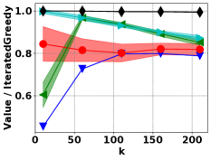
(a) Objective, BA

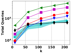
(b) Queries, BA

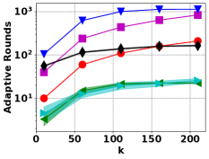
(c) Rounds, BA

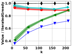
(d) Objective, ca-GrQc

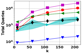
(e) Queries, ca-GrQc

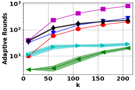
(f) Rounds, ca-GrQc

Figure 3: Additional results for maximum cut on BA and ca-GrQc. The legend in Fig. 1 applies.

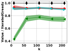
(a) Objective, small $k$

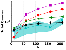
(b) Queries, small $k$

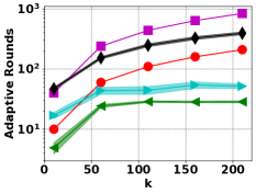
(c) Rounds, small $k$

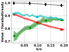
(d) Objective, large $k$

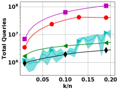
(e) Queries, large $k$

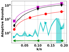
(f) Rounds, large $k$

Figure 4: Results for revenue maximization on ca-Astro, for both small and large $k$ values. Large $k$ values are indicated by a fraction of the total number $n$ of nodes. The legend is the same as in Fig. 1.

Results on additional datasets for the maximum cut application are shown in Figs. 3. These results are qualitatively similar to the ones discussed in Section 5. For the revenue maximization application, results on ca-Astro are shown in Figs. 4, for both small and large $k$ values. These results are qualitatively similar to the results for the maximum cut application.

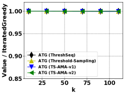
(a) Objective, BA

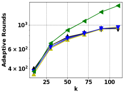
(b) Rounds, BA

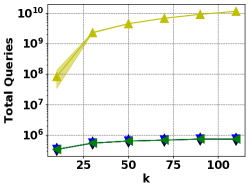
(c) Queries, ca-GrQc

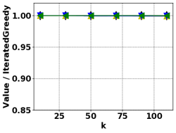
(d) Objective, ca-GrQc

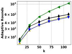
(e) Rounds, ca-GrQc

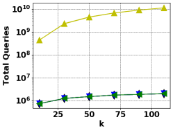
(f) Queries, ca-GrQc

Figure 5: Results of AST and ATG with four threshold procedures on two datasets. The algorithms are run strictly following pseudocode.

Comparison of ATG with different threshold sampling procedures. All ATG algorithms return the competitive solutions compared with IteratedGreedy; see Figs. 5(a) and 5(d). Since each iteration of ATG calls a threshold sampling subroutine which is based on the solution of previous iterations and a slowly decreasing threshold $\tau$, after the first filtration of the subroutine, the size of the candidate set is limited. Thus, there is no significant difference between different ATGs concerning rounds and queries. However, there are two exceptions. First, since TS-AMA-v2 is the only one who has $O\left(\log^{2}(n)\right)$ adaptive rounds, it still runs with more rounds; see Figs. 5(b) and 5(e). Also, the number of queries of ATG with Threshold-Sampling is significantly large with the same reason discussed in Section 5.

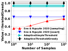
(a) Objective value

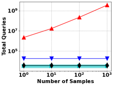
(b) Queries to set function

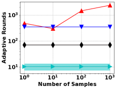
(c) Adaptive Rounds

Figure 6: Comparison of our algorithms with ?’s (?) on a very small random graph ($n=87$, $k=10$). In all plots, the $x$-axis shows the number of samples used to approximate the multilinear extension.

Approximation of the Multilinear Extension. In this section, we further investigate the performance of ?’s (?) when closed-form evaluation of the multilinear extension and its gradient are impossible. We find that sampling to approximate the multilinear extension and its gradient is extremely inefficient or yields poor solution quality with a small number of samples. For this reason, we exclude this algorithm from our revenue maximization experiments. To perform this evaluation, we compared versions of the algorithm of ?’s (?) that use varying number of samples to approximate the multilinear extension.

Results are shown in Fig. 6 on a very small random graph with $n=87$ and $k=10$. The figure shows the objective value and total queries to the set function vs. the number of samples used to approximate the multilinear extension. There is a clear tradeoff between the solution quality and the number of queries required; at $10^{3}$ samples per evaluation, the algorithm matches the objective value of the version with the exact oracle; however, even at roughly $10^{11}$ queries (corresponding to $10^{4}$ samples for each evaluation of the multilinear extension), the algorithm of ?’s (?) is unable to exceed $0.8$ of the IteratedGreedy value. On the other hand, if $\leq 10$ samples are used to approximate the multilinear extension, the algorithm is unable to exceed $0.5$ of the IteratedGreedy value and still requires on the order of $10^{7}$ queries.

G.3 Further Details of Algorithm Implementations

As stated above, we set $\varepsilon=0.1$ for all algorithms and used $100$ samples to evaluate expectations for adaptive algorithms. Further, in the algorithms AdaptiveSimpleThreshold, AdaptiveThresholdGreedy, and AdaptiveNonmonotoneMax, we ignored the smaller values of $\varepsilon$, $\delta$ passed to Threshold-Sampling in each algorithm, and simply used the input values of $\varepsilon$ and $\delta$.

For AdaptiveThresholdGreedy, we used an early termination condition to check if the threshold value $\tau<\textsc{OPT}(1-\varepsilon)/(ck)$, by using the best solution value found so far as a lower bound on OPT; this early termination condition is responsible for the high variance in total queries. We also used a sharper upper bound on $\textsc{OPT}/k$ in place of the maximum singleton: the sum of the top $k$ singleton values divided by $k$. We attempted to use the same sharper upper bound in AdaptiveNonmonotoneMax, but it resulted in signficantly worse objective values, so we simply used the maximum singleton as described in ?’s (?).

G.4 Multilinear Extension and Implementation of ?’s (?)

In this section, we describe the multilinear extension and implmentation of ?’s (?). The multilinear extension $F$ of set function $f$ is defined to be, for $x\in[0,1]^{n}$:

$$F(x)=\mathbb{E}\left[f(S)\right]=\sum_{S\subseteq V}f(S)Pr(S),$$

where

$$Pr(S)=\prod_{i\in S}x_{i}\cdot\prod_{i\not\in S}(1-x_{i}).$$

The gradient is approximated by using the central difference in each coordinate

$$\frac{dg}{dx}(x)\approx\frac{g(x+\gamma/2)-g(x-\gamma/2)}{\gamma},$$

unless using this approximation required evaluations outside the unit cube, in which case the forward or backward difference approximations were used. The parameter $\gamma$ is set to $0.5$.

Finally, for the maximum cut application, closed forms expressions exist for both the multilinear extension and its gradient. These are:

$$F(x)=\sum_{(u,v)\in E}x_{u}\cdot(1-x_{v})+x_{v}\cdot(1-x_{u}),$$

and

$$(\nabla F)_{u}=\sum_{v\in N(u)}(1-2x_{v}).$$

Implementation. The algorithm was implemented as specified in the pseudocode on page 19 of the arXiv version of ?’s (?). We followed the same parameter choices as in ?’s (?), although we set $\varepsilon=0.1$ as setting it to $0.05$ did not improve the objective value significantly but caused a large increase in runtime and adaptive rounds. The value of $\delta=\varepsilon^{3}$ was used after communications with the authors.

References

- Amanatidis et al. Amanatidis, G., Fusco, F., Lazos, P., Leonardi, S., Marchetti-Spaccamela, A., and Reiffenhäuser, R. (2021). Submodular maximization subject to a knapsack constraint: Combinatorial algorithms with near-optimal adaptive complexity. In International Conference on Machine Learning (ICML).
- Badanidiyuru and Vondrák Badanidiyuru, A., and Vondrák, J. (2014). Fast algorithms for maximizing submodular functions. In ACM-SIAM Symposium on Discrete Algorithms (SODA).
- Balkanski et al. Balkanski, E., Breuer, A., and Singer, Y. (2018). Non-monotone Submodular Maximization in Exponentially Fewer Iterations. In Advances in Neural Information Processing Systems (NeurIPS).
- Balkanski et al. Balkanski, E., Rubinstein, A., and Singer, Y. (2019). An Exponential Speedup in Parallel Running Time for Submodular Maximization without Loss in Approximation. In ACM-SIAM Symposium on Discrete Algorithms (SODA).
- Balkanski and Singer Balkanski, E., and Singer, Y. (2018). The adaptive complexity of maximizing a submodular function. In ACM SIGACT Symposium on Theory of Computing (STOC).
- Buchbinder and Feldman Buchbinder, N., and Feldman, M. (2016). Constrained Submodular Maximization via a Non-symmetric Technique. In Mathematics of Operations Research, Vol. 44.
- Buchbinder et al. Buchbinder, N., Feldman, M., Naor, J. S., and Schwartz, R. (2012). A Tight Linear Time (1 / 2)-Approximation for Unconstrained Submodular Maximization. In Symposium on Foundations of Computer Science (FOCS).
- Buchbinder et al. Buchbinder, N., Feldman, M., and Schwartz, R. (2015). Comparing Apples and Oranges: Query Tradeoff in Submodular Maximization. In ACM-SIAM Symposium on Discrete Algorithms (SODA).
- Chekuri and Quanrud Chekuri, C., and Quanrud, K. (2019). Parallelizing greedy for submodular set function maximization in matroids and beyond. In ACM SIGACT Symposium on Theory of Computing (STOC), pp. 78–89.
- Chen et al. Chen, L., Feldman, M., and Karbasi, A. (2019). Unconstrained submodular maximization with constant adaptive complexity. In ACM SIGACT Symposium on Theory of Computing (STOC), pp. 102–113.
- Chen et al. Chen, Y., Dey, T., and Kuhnle, A. (2021). Best of both worlds: Practical and theoretically optimal submodular maximization in parallel. In Advances in Neural Information Processing Systems (NeurIPS).
- El-Arini and Guestrin El-Arini, K., and Guestrin, C. (2011). Beyond Keyword Search: Discovering Relevant Scientific Literature. In ACM SIGKDD International Conference on Knowledge Discovery and Data Mining (KDD).
- Ene and Nguyen Ene, A., and Nguyen, H. L. (2019). Submodular Maximization with Nearly-optimal Approximation and Adaptivity in Nearly-linear Time. In ACM-SIAM Symposium on Discrete Algorithms (SODA).
- Ene and Nguyên Ene, A., and Nguyên, H. L. (2020). Parallel algorithm for non-monotone dr-submodular maximization. In International Conference on Machine Learning (ICML).
- Ene et al. Ene, A., Nguyên, H. L., and Vladu, A. (2019). Submodular maximization with matroid and packing constraints in parallel. In ACM SIGACT Symposium on Theory of Computing (STOC), pp. 90–101.
- Fahrbach et al. Fahrbach, M., Mirrokni, V., and Zadimoghaddam, M. (2019a). Non-monotone Submodular Maximization with Nearly Optimal Adaptivity Complexity. In International Conference on Machine Learning (ICML).
- Fahrbach et al. Fahrbach, M., Mirrokni, V., and Zadimoghaddam, M. (2019b). Submodular Maximization with Nearly Optimal Approximation, Adaptivity, and Query Complexity. In ACM-SIAM Symposium on Discrete Algorithms (SODA), pp. 255–273.
- Feige et al. Feige, U., Mirrokni, V., and Vondrák, J. (2011). Maximizing non-monotone submodular functions. In SIAM Journal on Computing.
- Gharan and Vondrák Gharan, S. O., and Vondrák, J. (2011). Submodular maximization by simulated annealing. In ACM-SIAM Symposium on Discrete Algorithms (SODA).
- Gupta et al. Gupta, A., Roth, A., Schoenebeck, G., and Talwar, K. (2010). Constrained non-monotone submodular maximization: Offline and secretary algorithms. In International Workshop on Internet and Network Economics (WINE), pp. 246–257.
- Hartline et al. Hartline, J., Mirrokni, V. S., and Sundararajan, M. (2008). Optimal marketing strategies over social networks. In International Conference on World Wide Web (WWW), pp. 189–198.
- Kazemi et al. Kazemi, E., Mitrovic, M., Zadimoghaddam, M., Lattanzi, S., and Karbasi, A. (2019). Submodular Streaming in All its Glory: Tight Approximation, Minimum Memory and Low Adaptive Complexity. In International Conference on Machine Learning (ICML).
- Kempe et al. Kempe, D., Kleinberg, J., and Tardos, É. (2003). Maximizing the spread of influence through a social network. In ACM SIGKDD International Conference on Knowledge Discovery and Data Mining (KDD).
- Kuhnle Kuhnle, A. (2021). Nearly linear-time, parallelizable algorithms for non-monotone submodular maximization. In AAAI Conference on Artificial Intelligence.
- Leskovec and Krevl Leskovec, J., and Krevl, A. (2020). SNAP Datasets: Stanford Large Network Dataset Collection. http://snap.stanford.edu/data.
- Libbrecht et al. Libbrecht, M. W., Bilmes, J. A., and Stafford, W. (2017). Choosing non-redundant representative subsets of protein sequence data sets using submodular optimization. In Proteins: Structure, Function, and Bioinformatics, No. July 2017, pp. 454–466.
- Mirzasoleiman et al. Mirzasoleiman, B., Badanidiyuru, A., and Karbasi, A. (2016). Fast Constrained Submodular Maximization : Personalized Data Summarization. In International Conference on Machine Learning (ICML).
- Mislove et al. Mislove, A., Koppula, H. S., Gummadi, K. P., Druschel, P., and Bhattacharjee, B. (2008). Growth of the Flickr Social Network. In First Workshop on Online Social Networks.
- Mitzenmacher and Upfal Mitzenmacher, M., and Upfal, E. (2017). Probability and computing: Randomization and probabilistic techniques in algorithms and data analysis. Cambridge university press.
- Nemhauser and Wolsey Nemhauser, G. L., and Wolsey, L. A. (1978). Best Algorithms for Approximating the Maximum of a Submodular Set Function.. Vol. 3, pp. 177–188.
- Simon et al. Simon, I., Snavely, N., and Seitz, S. M. (2007). Scene summarization for online image collections. In IEEE International Conference on Computer Vision (ICCV).
- Sipos et al. Sipos, R., Swaminathan, A., Shivaswamy, P., and Joachims, T. (2012). Temporal corpus summarization using submodular word coverage. In ACM International Conference on Information and Knowledge Management (CIKM).
- Tschiatschek et al. Tschiatschek, S., Iyer, R., Wei, H., and Bilmes, J. (2014). Learning Mixtures of Submodular Functions for Image Cxollection Summarization. In Advances in Neural Information Processing Systems (NeurIPS).