Optimal Control of Convection-Cooling and Numerical Implementation

Abstract

This paper is concerned with the problem of enhancing convection-cooling via active control of the incompressible velocity field, described by a stationary diffusion-convection model. This essentially leads to a bilinear optimal control problem. A rigorous proof of the existence of an optimal control is presented and the first order optimality conditions are derived for solving the control using a variational inequality. Moreover, the second order sufficient conditions are established to characterize the local minimizer. Finally, numerical experiments are conducted utilizing finite elements methods together with nonlinear iterative schemes, to demonstrate and validate the effectiveness of our control design.

1 Introduction

Convection-cooling is the mechanism where heat is transferred from the hot object into the surrounding air or liquid. There are several factors determining the effectiveness of cooling, including temperature difference between the surrounding and the hot object, viscosity of the fluid (air or liquid), and ability of the fluid to move in response to the density difference, etc. There are two types of convectional cooling, namely the natural convection cooling and the forced air convection cooling (cf. [3, 2, 19]). In the natural cooling, the air surrounding the object transfers the heat away from the object and does not use any fans or blowers. In contrast, forced air convection cooling is used in designs where the enclosures or environment do not offer an effective natural cooling performance and areas where natural cooling is not effective. The forced air convection cooling is the most effective cooling method in many industrial applications. It can be designed to provide the required cooling performance while increasing the efficiency of the related components.

The current work utilizes an optimal control approach for the forced air convection-cooling. To be more precise, consider a stationary diffusion-convection model for a cooling application in an open bounded and connected domain $\Omega\subset\mathbb{R}^{d},d=2,3$, with a Lipschitz boundary $\Gamma$. The velocity field is assumed to be divergence-free. The system of equations reads

$$-\kappa\Delta T+\mathbf{v}\cdot\nabla T =f\quad\text{in}\quad\Omega$$ (1.1)

$$\nabla\cdot\mathbf{v} =0,$$ (1.2)

with Dirichlet boundary condition for temperature and no-slip boundary condition for velocity

$$T|_{\Gamma} =0,\quad\mathbf{v}|_{\Gamma}=0,$$ (1.3)

where $T$ is the temperature, $\kappa>0$ is the thermal diffusivity, $\mathbf{v}$ is the velocity, and $f\in L^{\infty}(\Omega)$ is the external heat source distribution. The Dirichlet boundary condition is corresponding to a given fixed surface temperature, for example, when the surface is in contact with a melting solid or a boiling liquid. Although Neumann type of boundary conditions are often used in the diffusion-convection problems for describing heat flux at the boundaries, the Dirichlet boundary condition is also commonly employed in the study of natural convection and heat transfer in enclosures, which may be simultaneously heated from below and cooled from above (cf. [6, 10, 11, 22, 25]). Linear controls, either internal (distributed) or boundary controls, of the temperature and the corresponding numerical schemes have been well studied for diffusion-convection equations (cf. [4, 5, 7, 8, 9, 15, 18, 12, 26]). The objective of this work is aimed at enhancing convection-cooling via active control of the flow velocity. For example, in high power applications, a cooling fan is used to blow and direct air towards the electronic components with or without heat sinks. Most power supply units have built-in fans that provide the required forced-air convectional cooling. Mathematically, our control design gives rise to a bilinear optimal control problem.

Optimal control for enhancing heat transfer and fluid mixing or optic flow control via flow advection, governed by nonstationary diffusion-convection, has been discussed in (cf. [1, 16, 17, 21]). However, to solve the resulting nonlinear optimality system, one has to solve the state equations forward in time, coupled with the adjoint system backward in time together with a nonlinear optimality condition. This leads to extremely high computational costs and intractable problems. Some preliminary numerical results were obtained in [21] with simplified conditions. As a first step to tackle such a complex system, our current work will focus on the stationary case and present a rigorous theoretical and numerical study of the optimal control design.

Now denote the spatial average of temperature by

$$\langle T\rangle=\frac{1}{|\Omega|}\int_{\Omega}T\,dx.$$

The objective is to minimize the variance of the temperature with optimal control cost, that is,

$$J({\mathbf{v}}) =\frac{1}{2}\|T-\langle T\rangle\|^{2}_{L^{2}}+\frac{\gamma}{2}\|\mathbf{v}\|^{2}_{U_{\text{ad}}},\qquad(P)$$

subject to (1.1)–(1.3), where $\gamma>0$ is the control weight parameter and $U_{\text{ad}}$ stands for the set of admissible control. The choice of the set of admissible control is usually dependent on the physical properties and the need to establish the existence of an optimal control. Due to the advection term $\mathbf{v}\cdot\nabla T$, the control map $\mathbf{v}\mapsto T$ is bilinear and hence problem $(P)$ is non-convex. Establishing the existence of an optimal velocity field will involve a compactness argument associated with the control map. Moreover, in order to reduce the effects of rotation on the flow and the shear stress at the boundary in the cooling process, we consider to minimize the magnitude of the strain tensor (cf. [14]), which is equivalent to minimize $\|\nabla\mathbf{v}\|_{L^{2}}$. To this end, we set

$$U_{\text{ad}}=\{\mathbf{v}\in H^{1}_{0}(\Omega)\colon\nabla\cdot\mathbf{v}=0\}$$

equipped with $H^{1}$-norm

$$\|\mathbf{v}\|_{U_{\text{ad}}}=\|\mathbf{v}\|_{H^{1}}.$$

The remainder of this paper is organized as follows. Section 2 focuses on the existence of an optimal solution to problem $(P)$. Section 3 presents the first and second order optimality conditions for solving and charactering the optimal solution by using a variational inequality (cf. [20]). Moreover, it can be shown that there exists a strict local minimizer if the control weight $\gamma$ is large enough. Section 4 discusses the numerical implementation of our control design, where the finite element formulation and nonlinear iterative solvers are used to construct our numerical schemes. In particular, the relation regarding the solutions of the optimality system associated with different values in $\kappa$ and $\gamma$ is established. This result provides a practical guidance for choosing these parameters in our numerical implementation. In Section 5, several numerical experiments are conducted to demonstrate the effectiveness of our control design for convection-cooling. Lastly, this paper concludes with potential problems for future work in Section 6.

In the sequel, the symbol $C$ denotes a generic positive constant, which is allowed to depend on the domain as well as on indicated parameters without ambiguous.

2 Existence of an Optimal Solution

As a starting point to analyze problem $(P)$, we first recall some basic properties of the state equations (1.1)–(1.3). The following lemmas will be often used in this paper.

Lemma 2.1.

Let $\mathbf{w}\in(H^{1}(\Omega))^{d},d=2,3$, and $\phi,\psi\in H^{1}(\Omega)$. Then we have

$$\left|\int_{\Omega}\mathbf{w}\cdot\nabla\phi\psi\,dx\right|\leq\|\mathbf{w}\|_{L^{4}}\|\nabla\phi\|_{L^{2}}\|\psi\|_{L^{4}}\leq C\|\nabla\mathbf{w}\|_{L^{2}}\|\nabla\phi\|_{L^{2}}\|\nabla\psi\|_{L^{2}}.$$ (2.1)

Moreover, if $\nabla\cdot\mathbf{w}=0$ and $\mathbf{w}|_{\Gamma}=0$, then

$$\int_{\Omega}\mathbf{w}\cdot\nabla\phi\psi\,dx=-\int_{\Omega}\phi\mathbf{w}\cdot\nabla\psi\,dx.$$ (2.2)

Proof.

Inequalities in (2.1) are direct results of Hölder’s inequality and Sobolev embedding theorem (cf. [24]). To see (2.2), applying Stokes formula together with $\nabla\cdot\mathbf{w}=0$ and $\mathbf{w}|_{\Gamma}=0$ follows

$$\int_{\Omega}\mathbf{w}\cdot\nabla\phi\psi\,dx =\int_{\Omega}\mathbf{w}\cdot\nabla(\phi\psi)\,dx-\int_{\Omega}\phi\mathbf{w}\cdot\nabla\psi\,dx$$

$$=\int_{\Gamma}\mathbf{w}\cdot n(\phi\psi)\,dx-\int_{\Omega}\nabla\cdot\mathbf{w}\phi\psi\,dx-\int_{\Omega}\phi\mathbf{w}\cdot\nabla\psi\,dx$$

$$=-\int_{\Omega}\phi\mathbf{w}\cdot\nabla\psi\,dx.$$

∎

Lemma 2.2.

Let $f\in L^{\infty}(\Omega)$. For $\mathbf{v}\in L^{2}(\Omega)$ with $\nabla\cdot\mathbf{v}=0$ and $\mathbf{v}|_{\Gamma}=0$, there exists a unique weak solution to equation (1.1) with Dirichlet boundary condition $T|_{\Gamma}=0$, which satisfies $T\in H^{1}_{0}(\Omega)\cap L^{\infty}(\Omega)$. Moreover,

$$\|T\|_{L^{2}}+\|\nabla T\|_{L^{2}}\leq\frac{C}{\kappa}\|f\|_{L^{2}}$$ (2.3)

and

$$\|T\|_{L^{\infty}}\leq C\|f\|_{L^{\infty}},$$ (2.4)

where $C>0$ depends on $\Omega$ but not on $f$.

Proof.

The existence of a unique solution follows the standard approaches for the elliptic equations (cf. [13]). To see (2.3), taking the inner product of (1.1) with $T$ and integrating by parts using (1.3), we have

$$\kappa\|\nabla T\|^{2}_{L^{2}} =-\int_{\Omega}(\mathbf{v}\cdot\nabla T)T\,dx+\int_{\Omega}fT\,dx$$

$$\leq-\frac{1}{2}\int_{\Omega}\mathbf{v}\cdot\nabla(T^{2})\,dx+\|f\|_{L^{2}}\|T\|_{L^{2}}$$

$$=-\frac{1}{2}(\int_{\Gamma}\mathbf{v}\cdot n\,T^{2}\,dx-\int_{\Omega}\nabla\cdot\mathbf{v}\,T^{2}\,dx)+\|f\|_{L^{2}}\|T\|_{L^{2}}$$

$$=\|f\|_{L^{2}}\|T\|_{L^{2}}\leq C\|f\|_{L^{2}}\|\nabla T\|_{L^{2}},$$ (2.5)

which follows

$$\|\nabla T\|_{L^{2}}\leq\frac{C}{\kappa}\|f\|_{L^{2}}.$$

Note that in (2.5) we have used Poncaré inequality $\|T\|_{L^{2}}\leq C\|\nabla T\|_{L^{2}}$, where $C>0$ is a constant dependent on domain $\Omega$ but not $f$.

Analogously, taking the inner product of (1.1) with $T^{N-1}$ for a positive even integer $N$ and then letting $N\to\infty$ we get (2.4). In fact, a finer estimate of $f$ in (2.4) can be achieved by using the Stampacchia theory. The reader is referred to [23] for details. This completes the proof. ∎

To show the existence of an optimal control to problem $(P)$, we first introduce the weak solution to (1.1)–(1.3).

Definition 2.3.

Let $f\in L^{\infty}(\Omega)$ and $\mathbf{v}\in U_{\text{ad}}$. $T\in H^{1}_{0}(\Omega)$ is said to be a weak solution to system (1.1)–(1.3), if $T$ satisfies

$$\kappa(\nabla T,\nabla\psi)-(T\mathbf{v},\nabla\psi) =(f,\psi),\quad\forall\psi\in H^{1}_{0}(\Omega).$$ (2.6)

Theorem 2.4.

For $f\in L^{\infty}(\Omega)$, there exists an optimal velocity $\mathbf{v}\in U_{\text{ad}}$ to problem $(P)$.

Proof.

Since $J$ is bounded from below, we may choose a minimizing sequence $\{\mathbf{v}_{m}\}\subset U_{\text{ad}_{1}}$ such that

$$\lim_{m\to\infty}J(\mathbf{v}_{m})=\inf_{\mathbf{v}\in U_{\text{ad}}}J(\mathbf{v}).$$ (2.7)

This also indicates that $\{\mathbf{v}_{m}\}$ is uniformly bounded in $U_{\text{ad}}$, and hence there exists a weakly convergent subsequence, still denoted by $\{\mathbf{v}_{m}\}$, such that

$$\mathbf{v}_{m}\to\mathbf{v}^{*}\quad\text{weakly in}\quad H^{1}(\Omega),\ \ \text{as}\ \ m\to\infty,$$ (2.8)

$$\mathbf{v}_{m}\to\mathbf{v}^{*}\quad\text{strongly in}\quad L^{2}(\Omega),\ \ \text{as}\ \ m\to\infty.$$ (2.9)

Let $\{T_{m}\}$ be the solutions corresponding to $\{\mathbf{v}_{m}\}$. Then $\{T_{m}\}$ is uniformly bounded in $H^{1}(\Omega)\cap L^{\infty}(\Omega)$ according to (2.3) and (2.4) . Thus there exists a subsequence, still denoted by $\{T_{m}\}$, satisfying

$$T_{m}\to T^{*}\quad\text{weakly in}\ H^{1}(\Omega),\ \text{as}\ \ m\to\infty,$$ (2.10)

$$T_{m}\to T^{*}\quad\text{weakly* in}\ L^{\infty}(\Omega),\ \text{as}\ \ m\to\infty.$$ (2.11)

Next we show that $T^{*}$ is the solution corresponding to $\mathbf{v}^{opt}$ by Definition 2.3. Recall that $\mathbf{v}_{m}$ and $T_{m}$ satisfy

$$\kappa(\nabla T_{m},\nabla\psi)-(T_{m}\mathbf{v}_{m},\nabla\psi)=(f,\psi),\quad\forall\psi\in H^{1}_{0}(\Omega),$$ (2.12)

With the help of (2.10), it is easy to pass to the limit in the first term on the left hand of (2.12). Next we show that applying (2.8)–(2.9) and (2.11) makes passing to the limit in the nonlinear term $\mathbf{v}_{m}T_{m}\to\mathbf{v}^{*}T^{*}$ possible.

In fact, for the second term on the left hand of (2.12), we have for $\psi\in H^{1}_{0}(\Omega)$,

$$\left|\int_{\Omega}T_{m}\mathbf{v}_{m}\cdot\nabla\psi\,dx-\int_{\Omega}T^{*}\mathbf{v}^{*}\cdot\nabla\psi\,dx\right|$$

$$\quad\leq\left|\int_{\Omega}T_{m}\mathbf{v}_{m}\cdot\nabla\psi-T_{m}\mathbf{v}^{*}\cdot\nabla\psi\,dx\right|$$

$$\qquad+\left|\int_{\Omega}T_{m}\mathbf{v}^{*}\cdot\nabla\psi-T^{*}\mathbf{v}^{*}\cdot\nabla\psi\,dx\right|$$

$$\quad=I_{1}+I_{2},$$ (2.13)

where

$$I_{1} \leq\|T_{m}\|_{L^{\infty}}\|\mathbf{v}_{m}-\mathbf{v}^{*}\|_{L^{2}}\|\nabla\psi\|_{L^{2}}\to 0\quad\text{as}\quad m\to\infty,$$

due to (2.9) and the uniform boundedness of $\|T_{m}\|_{L^{\infty}}$. Moreover, $I_{2}\to 0$ due to (2.11) and $\mathbf{v}^{*}\nabla\psi\in L^{1}(\Omega)$. Clearly, $T^{*}\in H^{1}_{0}(\Omega)$ is the solution corresponding to $\mathbf{v}^{*}$ based on Definition 2.3.

Lastly, using the weakly lower semicontinuity property of norms yields

$$\|\mathbf{v}^{*}\|_{U_{\text{ad}}}\leq\displaystyle\varliminf_{m\to\infty}\|\mathbf{v}_{m}\|_{U_{\text{ad}}}\quad\text{and}\quad\|T^{*}-\langle T^{*}\rangle\|_{L^{2}}\leq\varliminf_{m\to\infty}\|T_{m}-\langle T_{m}\rangle\|_{L^{2}}.$$

In other words,

$$J(\mathbf{v}^{*})\leq\varliminf_{m\to\infty}J(\mathbf{v}_{m})=\inf_{\mathbf{v}\in U_{\text{ad}}}J(\mathbf{v}),$$

which indicates that $\mathbf{v}^{*}$ is an optimal solution to problem $(P)$. ∎

3 Optimality Conditions

Now we derive the first order necessary optimality conditions for problem $(P)$ by using a variational inequality (cf. [20]), that is, if $\mathbf{v}$ is an optimal solution to problem $(P)$, then

$$J^{\prime}(\mathbf{v})\cdot(\psi-\mathbf{v})\geq 0,\quad\psi\in U_{\text{ad}}.$$ (3.1)

To establish the G$\hat{a}$teaux differentiability of $J(\mathbf{v})$, we first check the G$\hat{a}$teaux differentiability of $T$ with respect to $\mathbf{v}$. Let $z$ be the G$\hat{a}$teaux of $T$ with respect to $\mathbf{v}$ in the direction of $h\in U_{\text{ad}}$, i.e., $z=T^{\prime}(\mathbf{v})\cdot h$. Then $z$ satisfies

$$\begin{split}-\kappa\Delta z+\mathbf{v}\cdot\nabla z+h\cdot\nabla T&=0,\\ \ z|_{\Gamma}&=0.\end{split}$$ (3.2)

Using the $L^{2}$-estimate as in Lemma 2.2 with the help of Lemma 2.1 and (2.3), we get

$$\kappa\|\nabla z\|^{2}_{L^{2}} \leq\left|\int_{\Omega}(h\cdot\nabla T)z\,dx\right|\leq C\|\nabla h\|_{L^{2}}\|\nabla T\|_{L^{2}}\|\nabla z\|_{L^{2}},$$ (3.3)

which implies

$$\|\nabla z\|_{L^{2}} \leq\frac{C}{\kappa}\|\nabla h\|_{L^{2}}\|\nabla T\|_{L^{2}}\leq\frac{C}{\kappa^{2}}\|f\|_{L^{2}}\|\nabla h\|_{L^{2}}.$$ (3.4)

Therefore, $T(\mathbf{v})$ is G$\hat{a}$teaux differentiable for $\mathbf{v}\in U_{\text{ad}}$, so is $J(\mathbf{v})$.

3.1 First Order Optimality Conditions

Let $A=-\mathbb{P}\Delta$ be the Stokes operator with

$$D(A)=\{H^{1}_{0}(\Omega)\cap H^{2}(\Omega)\colon\nabla\cdot\mathbf{v}=0\},$$

where $\mathbb{P}\colon L^{2}(\Omega)\to\{\mathbf{v}\in L^{2}(\Omega)\colon\nabla\cdot\mathbf{v}=0\ \text{and}\ \mathbf{v}\cdot\textbf{n}|_{\Gamma}=0\}$ is the Leray projector. Note that $A$ is a strictly positive and self-adjoint operator. Moreover, define operator $D\colon L^{2}(\Omega)\to L^{2}(\Omega)$ by $DT=T-\langle T\rangle$. Then $D$ is a bounded linear operator. The cost functional now can be rewritten as

$$J(\mathbf{v}) =\frac{1}{2}(D^{*}DT,T)+\frac{\gamma}{2}(A\mathbf{v},\mathbf{v}),$$ (3.5)

where $D^{*}$ is the $L^{2}$-adjoint operator of $D$.

Remark 3.5.

Here we present some basic properties of operator $D$. For any $T,\psi\in L^{2}(\Omega)$, since $\langle T\rangle$ and $\langle\psi\rangle$ are constants, we have

$$\frac{1}{|\Omega|}\int_{\Omega}T\langle\psi\rangle\,dx=\langle T\rangle\langle\psi\rangle=\frac{1}{|\Omega|}\int_{\Omega}\langle T\rangle\psi\,dx.$$

Therefore,

$$(DT,\psi) =\int_{\Omega}(T-\langle T\rangle)\psi\,dx=\int_{\Omega}T\psi\,dx-\int_{\Omega}\langle T\rangle\psi\,dx$$

$$=\int_{\Omega}T\psi\,dx-\int_{\Omega}T\langle\psi\rangle\,dx=(T,\psi-\langle\psi\rangle)=(T,D\psi),$$

which says that $D$ is a self-adjoint operator on $L^{2}(\Omega)$, i.e., $D=D^{*}$. Moreover, since

$$\langle T-\langle T\rangle\rangle=\frac{1}{|\Omega|}\int_{\Omega}(T-\langle T\rangle)\,dx=\langle T\rangle-\langle T\rangle=0,$$

it is straightforward to verify that

$$D^{*}DT =D(DT)=D(T-\langle T\rangle)=T-\langle T\rangle-\langle T-\langle T\rangle\rangle=DT,$$

which implies that $D^{2}=D$, and hence the operator norm $\|D\|\leq 1$.

Now let $q$ be the adjoint state associated with $T$. Then it is easy to verify that $q$ satisfies

$$\begin{split}-\kappa\Delta q-\mathbf{v}\cdot\nabla q&=D^{*}DT\quad\mbox{in }\Omega,\\ \ q|_{\Gamma}&=0.\end{split}$$ (3.6)

Moreover, thanks to (2.3) and $\|D\|\leq 1$, we have

$$\|\nabla q\|_{L^{2}} \leq\frac{C}{\kappa}\|T\|_{L^{2}}\leq\frac{C}{\kappa^{2}}\|f\|_{L^{2}}.$$ (3.7)

The following theorem establishes the first order necessary optimality conditions for solving the optimal solution.

Theorem 3.6.

Assume that $\mathbf{v}^{\text{opt}}$ is an optimal solution to problem $(P)$. Let $(T^{opt},q^{opt})$ be the corresponding solution to the state equations (1.1)–(1.3) and the adjoint system (3.6). Then $(\mathbf{v}^{\text{opt}},T^{opt},q^{opt})$ satisfies

$$\begin{cases}-\kappa\Delta T+{\mathbf{v}}\cdot\nabla T=f\quad\text{ and }\quad T|_{\partial\Omega}=0,\\ -\kappa\Delta q-{\mathbf{v}}\cdot\nabla q=D^{*}DT\quad\text{ and }\quad q|_{\partial\Omega}=0,\\ -\gamma\Delta{\mathbf{v}}+\nabla p=q\nabla T,\quad\nabla\cdot\mathbf{v}=0\quad\text{ and }\quad\mathbf{v}|_{\partial\Omega}=0.\end{cases}$$ (3.8)

Proof.

In light of (3.5), (3.6), and (2.2), the Gâteaux derivative of $J$ becomes

$$J^{\prime}(\mathbf{v})\cdot h= (D^{*}DT,z)+\gamma(A\mathbf{v},h)$$

$$= (-\kappa\Delta q-\mathbf{v}\cdot\nabla q,z)+\gamma(A\mathbf{v},h)$$

$$= (q,-\kappa\Delta z+\mathbf{v}\cdot\nabla z)+\gamma(A\mathbf{v},h).$$

Using (3.2) we get

$$J^{\prime}(\mathbf{v})\cdot h= -(q,h\cdot\nabla T)+\gamma(A\mathbf{v},h).$$

If $\mathbf{v}^{\text{opt}}$ is the optimal solution, then $J^{\prime}(\mathbf{v}^{\text{opt}})\cdot h\geq 0$ for any $h\in U_{\text{ad}}$. This yields the following optimality condition

$$\gamma A\mathbf{v}^{\text{opt}}-\mathbb{P}(q\nabla T)=0.$$ (3.9)

In other words, there exists $p\in L^{2}(\Omega)$ with $\int_{\Omega}p\,dx=0$ such that

$$-\gamma\Delta\mathbf{v}^{\text{opt}}+\nabla p=q\nabla T,$$

which completes the proof. ∎

3.2 Second Order Optimality Conditions

In this section, we discuss the second order optimality conditions for characterizing the optimal velocity field. In particular, it can be shown that the cost functional $J$ has a strict local minimizer when the control weight $\gamma>0$ is sufficiently large.

Theorem 3.7.

Let $(\mathbf{v},T,q)$ satisfy the first order necessary optimality system (3.8). If $\gamma>0$ is sufficiently large, then there exists some constant $\delta>0$ such that

$$J^{\prime\prime}(\mathbf{v})\cdot(h,h)\geq\delta\|h\|_{U_{\text{ad}}},$$ (3.10)

for $h\in U_{\text{ad}}$ satisfying (3.2).

Proof.

Let $h_{i}\in U_{\text{ad}}$ and $z_{i}=T^{\prime}(\mathbf{v})\cdot h_{i},i=1,2$. Then we have

$$\begin{split}-\kappa\Delta z_{i}+\mathbf{v}\cdot\nabla z_{i}+h_{i}\cdot\nabla T&=0\quad\mbox{in }\Omega,\\ \ z_{i}|_{\Gamma}&=0.\end{split}$$

Moreover, let $Z=z^{\prime}_{1}(\mathbf{v})\cdot h_{2}$. Then $Z$ satisfies

$$-\kappa\Delta Z+h_{2}\cdot\nabla z_{1}+\mathbf{v}\cdot\nabla Z+h_{1}\cdot\nabla z_{2} =0\quad\mbox{in }\Omega,$$ (3.11)

$$Z|_{\Gamma} =0.$$

Again applying an $L^{2}$-estimate for $Z$ and using (3.4), we can easily verify that

$$\|\nabla Z\|_{L^{2}} \leq\frac{C}{\kappa}(\|\nabla h_{2}\|_{L^{2}}\|\nabla z_{1}\|_{L^{2}}+\|\nabla h_{1}\|_{L^{2}}\|\nabla z_{2}\|_{L^{2}})$$

$$\leq\frac{C}{\kappa^{3}}\|f\|_{L^{2}}\|\nabla h_{1}\|_{L^{2}}\|\nabla h_{2}\|_{L^{2}},$$ (3.12)

which implies that $T(\mathbf{v})$ is twice G$\hat{a}$teaux differentiable for $\mathbf{v}\in U_{\text{ad}}$, so is $J(\mathbf{v})$.

Now differentiating $J^{\prime}(\mathbf{v})\cdot h_{1}$ once again in the direction $h_{2}\in U_{\text{ad}}$ gives

$$J^{\prime\prime}(\mathbf{v})\cdot(h_{1},h_{2})=(D^{*}Dz_{2},z_{1})+(D^{*}DT,Z)+\gamma(Ah_{2},h_{1}).$$ (3.13)

To further analyze the second term involving $Z$, we take the inner product of (3.11) with $q$ and apply (2.2). We get

$$-\kappa(Z,\Delta q)-(z_{1},h_{2}\cdot\nabla q)-(Z,\mathbf{v}\cdot\nabla q)-(z_{2},h_{1}\cdot\nabla q)=0.$$

With the help of the adjoint equation (3.6), we obtain

$$(z_{1},h_{2}\cdot\nabla q)+(z_{2},h_{1}\cdot\nabla q)=(Z,D^{*}DT).$$

Therefore,

$$J^{\prime\prime}(\mathbf{v})\cdot(h_{1},h_{2})= (D^{*}Dz_{2},z_{1})+(z_{1},h_{2}\cdot\nabla q)+(z_{2},h_{1}\cdot\nabla q)+\gamma(Ah_{2},h_{1}).$$

Setting $h_{1}=h_{2}=h$ and $z_{1}=z_{2}=z=T^{\prime}(\mathbf{v})\cdot h$ follows

$$J^{\prime\prime}(\mathbf{v})\cdot(h,h)=\|Dz\|^{2}_{L^{2}}+2(z,h\cdot\nabla q)+\gamma\|A^{1/2}h\|^{2}_{L^{2}}.$$ (3.14)

Furthermore, by (2.1), (3.4) and (3.7), we get

$$|\int_{\Omega}zh\cdot\nabla q\,dx|\leq C\|\nabla z\|_{L^{2}}\|\nabla h\|_{L^{2}}\|\nabla q\|_{L^{2}}\leq\frac{C}{\kappa^{4}}\|f\|^{2}_{L^{2}}\|A^{1/2}h\|^{2}_{L^{2}}$$

and

$$\|Dz\|_{L^{2}}\leq C\|\nabla z\|_{L^{2}}\leq\dfrac{C}{\kappa^{2}}\|f\|_{L^{2}}\|A^{1/2}h\|_{L^{2}}.$$

Consequently,

$$|J^{\prime\prime}(\mathbf{v})\cdot(h,h)| \leq\frac{C}{\kappa^{4}}\|f\|^{2}_{L^{2}}\|A^{1/2}h\|^{2}_{L^{2}}+\gamma\|A^{1/2}h\|^{2}_{L^{2}}=(\frac{C}{\kappa^{4}}\|f\|^{2}_{L^{2}}+\gamma)\|A^{1/2}h\|^{2}_{L^{2}}$$ (3.15)

and

$$J^{\prime\prime}(\mathbf{v})\cdot(h,h)\geq -2|(z,h\cdot\nabla q)|+\gamma\|A^{1/2}h\|^{2}_{L^{2}}=(\gamma-\frac{C}{\kappa^{4}}\|f\|^{2}_{L^{2}})\|A^{1/2}h\|^{2}_{L^{2}}.$$ (3.16)

Therefore, if $\gamma$ is large enough such that

$$\gamma-\frac{C}{\kappa^{4}}\|f\|^{2}_{L^{2}}\geq\delta>0,$$ (3.17)

then (3.10) holds. ∎

Lemma 3.8.

There exists a constant $C>0$ such that

$$|(J^{\prime\prime}(\mathbf{v}_{1})-J^{\prime\prime}(\mathbf{v}_{2}))\cdot(h,h)|\leq\frac{C}{\kappa^{5}}\|\mathbf{v}_{1}-\mathbf{v}_{2}\|_{H^{1}}\|f\|^{2}_{L^{2}}\|h\|^{2}_{H^{1}},$$ (3.18)

for any $h,\mathbf{v}_{i}\in U_{\text{ad}},i=1,2$.

Proof.

Let $h,\mathbf{v}_{i}\in U_{\text{ad}}$ and $z_{i}=T^{\prime}_{i}(\mathbf{v}_{i})\cdot h,i=1,2$. Here $T_{i}$ is the temperature corresponding to $\mathbf{v}_{i}$. Then $z_{i}$ satisfies

$$\begin{split}-\kappa\Delta z_{i}+\mathbf{v}_{i}\cdot\nabla z_{i}+h\cdot\nabla T_{i}&=0\quad\mbox{in }\Omega,\\ \ z_{i}|_{\Gamma}&=0.\end{split}$$

Further let $\tilde{z}=z_{1}-z_{2}$, $\tilde{\mathbf{v}}=\mathbf{v}_{1}-\mathbf{v}_{2}$ and $\tilde{T}=T_{1}-T_{2}$. Then

$$\begin{split}-\kappa\Delta\tilde{z}+\tilde{\mathbf{v}}\cdot\nabla z_{1}+\mathbf{v}_{2}\cdot\nabla\tilde{z}+h\cdot\nabla\tilde{T}&=0\quad\mbox{in }\Omega,\\ \ \tilde{z}|_{\Gamma}&=0.\end{split}$$ (3.19)

By (1.1)-(1.3) and (2.3) it is easy to check that

$$\|\tilde{T}\|_{H^{1}}\leq\frac{C}{\kappa}\|\tilde{\mathbf{v}}\|_{H^{1}}\|T\|_{H^{1}}\leq\frac{C}{\kappa^{2}}\|\tilde{\mathbf{v}}\|_{H^{1}}\|f\|_{L^{2}}.$$ (3.20)

Moreover, applying an $L^{2}$-estimate to (3.19) yields

$$\|\nabla\tilde{z}\|_{L^{2}} \leq\frac{C}{k}(\|\tilde{\mathbf{v}}\|_{H^{1}}\|z_{1}\|_{H^{1}}+\|h\|_{H^{1}}\|\tilde{T}\|_{H^{1}})$$

$$\leq\frac{C}{k}\left(\|\tilde{\mathbf{v}}\|_{H^{1}}\frac{C}{\kappa^{2}}\|f\|_{L^{2}}\|h\|_{H^{1}}+\|h\|_{H^{1}}\frac{C}{\kappa^{2}}\|\tilde{\mathbf{v}}\|_{H^{1}}\|f\|_{L^{2}}\right)$$

$$\leq\frac{C}{\kappa^{3}}\|\tilde{\mathbf{v}}\|_{H^{1}}\|f\|_{L^{2}}\|h\|_{H^{1}}.$$ (3.21)

Now let $Z_{i}=z^{\prime}_{i}(\mathbf{v}_{i})\cdot h,i=1,2,$. Then

$$\begin{split}-\kappa\Delta Z_{i}+2h\cdot\nabla z_{i}+\mathbf{v}_{i}\cdot\nabla Z_{i}&=0\quad\mbox{in }\Omega,\\ \ Z_{i}|_{\Gamma}&=0.\end{split}$$

In light of (3.12), we have

$$\|\nabla Z_{i}\|_{L^{2}}\leq\frac{C}{\kappa^{3}}\|f\|_{L^{2}}\|\nabla h\|^{2}_{L^{2}}.$$ (3.22)

Furthermore, let $\tilde{Z}=Z_{1}-Z_{2}$. Then

$$\begin{split}-\kappa\Delta\tilde{Z}+2h\cdot\nabla\tilde{z}+\tilde{\mathbf{v}}\cdot\nabla Z_{1}+\mathbf{v}_{2}\cdot\nabla\tilde{Z}&=0\quad\mbox{in }\Omega,\\ \ \tilde{Z}|_{\Gamma}&=0.\end{split}$$ (3.23)

Again applying an $L^{2}$-estimate to (3.23) and using (3.21)-(3.22) follow

$$\|\nabla\tilde{Z}\|_{L^{2}} \leq\frac{C}{\kappa}(2\|h\|_{H^{1}}\|\tilde{z}\|_{H^{1}}+\|\tilde{\mathbf{v}}\|_{H^{1}}\|Z_{1}\|_{H^{1}})$$

$$\leq\frac{C}{\kappa}\left(2\|h\|_{H^{1}}\frac{C}{\kappa^{3}}\|\tilde{\mathbf{v}}\|_{H^{1}}\|f\|_{L^{2}}\|h\|_{H^{1}}+\|\tilde{\mathbf{v}}\|_{H^{1}}\frac{C}{\kappa^{3}}\|f\|_{L^{2}}\|h\|^{2}_{H^{1}}\right)$$

$$\leq\frac{C}{\kappa^{4}}\|\tilde{\mathbf{v}}\|_{H^{1}}\|f\|_{L^{2}}\|h\|^{2}_{H^{1}}.$$ (3.24)

Finally, applying (3.13) together with (2.3), (3.4), (3.21)-(3.22), (3.24) and $\|D\|\leq 1$ follows

$$|(J^{\prime\prime}(\mathbf{v}_{1})-J^{\prime\prime}(\mathbf{v}_{2}))\cdot(h,h)|=\|Dz_{1}\|^{2}_{L^{2}}+(D^{*}DT,Z_{1})+\gamma\|A^{1/2}h\|^{2}_{L^{2}}$$

$$\qquad\quad-(\|Dz_{2}\|^{2}_{L^{2}}+(D^{*}DT,Z_{2})+\gamma\|A^{1/2}h\|^{2}_{L^{2}})$$

$$\qquad=(\|Dz_{1}\|^{2}_{L^{2}}-\|Dz_{2}\|^{2}_{L^{2}})+(D^{*}DT,Z_{1}-Z_{2})$$

$$\qquad\leq(\|z_{1}\|_{L^{2}}+\|z_{2}\|_{L^{2}})\|z_{1}-z_{2}\|_{L^{2}}+\|T\|_{L^{2}}\|Z_{1}-Z_{2}\|_{L^{2}}$$

$$\qquad\leq\frac{C}{\kappa^{2}}\|f\|_{L^{2}}\|h\|_{H^{1}}\frac{C}{\kappa^{3}}\|\tilde{\mathbf{v}}\|_{H^{1}}\|f\|_{L^{2}}\|h\|_{H^{1}}+\frac{C}{\kappa}\|f\|_{L^{2}}\frac{C}{\kappa^{4}}\|\tilde{\mathbf{v}}\|_{H^{1}}\|f\|_{L^{2}}\|h\|^{2}_{H^{1}}$$

$$\qquad\leq\frac{C}{\kappa^{5}}\|\tilde{\mathbf{v}}\|_{H^{1}}\|f\|^{2}_{L^{2}}\|h\|^{2}_{H^{1}},$$

which establishes the desired result. ∎

Now we are in a position to address the second order sufficient conditions. Let $\mathbf{w}\in U_{\text{ad}}$ and $T$ be the associated solution to (1.1)–(1.3). Define

$$\mathbb{T}(\mathbf{w})=\{\mathbf{v}\in U_{\text{ad}} \colon z=T^{\prime}(\mathbf{w})\cdot(\mathbf{v}-\mathbf{w})\ \text{satisfies}$$

$$-\kappa\Delta z+\mathbf{w}\cdot\nabla z+(\mathbf{v}-\mathbf{w})\cdot\nabla T=0,\ z|_{\Gamma}=0\}.$$

Corollary 3.9.

Let $\mathbf{v}^{*}$ satisfy the optimality condition (3.9). If $\gamma>0$ is sufficiently large, then there exist $\epsilon,\delta_{0}>0$ such that the quadratic growth condition

$$J(\mathbf{v}^{*})+\delta_{0}\|\mathbf{v}-\mathbf{v}^{*}\|^{2}_{U_{\text{ad}}}\leq J(\mathbf{v})$$ (3.25)

holds for all $\mathbf{v}\in\mathbb{T}(\mathbf{v}^{*})$ and $\|\mathbf{v}-\mathbf{v}^{*}\|_{H^{1}}\leq\epsilon$. In particular, $J$ has a local minimum in $\mathbb{T}(\mathbf{v}^{*})$ at $\mathbf{v}^{*}$.

Proof.

To see the gap between $J(\mathbf{v}^{*})$ and $J(\mathbf{v})$ for any $\mathbf{v}\in\mathbb{T}(\mathbf{v}^{*})$ satisfying $\|\mathbf{v}-\mathbf{v}^{*}\|_{H^{1}}\leq\epsilon$, we apply a Taylor expansion of $J(\mathbf{v})$ around $\mathbf{v}^{*}$. With the help of Theorem 3.7 and Lemma 3.8 and setting $h=\mathbf{v}-\mathbf{v}^{*}$, we have for $\xi\in(0,1)$,

$$J(\mathbf{v})-J(\mathbf{v}^{*}) =J^{\prime}(\mathbf{v}^{*})\cdot(\mathbf{v}-\mathbf{v}^{*})+\frac{1}{2}J^{\prime\prime}(\mathbf{v}^{*}+\xi(\mathbf{v}-\mathbf{v}^{*}))\cdot(\mathbf{v}-\mathbf{v}^{*},\mathbf{v}-\mathbf{v}^{*})$$

$$=\frac{1}{2}J^{\prime\prime}(\mathbf{v}^{*})\cdot(\mathbf{v}-\mathbf{v}^{*},\mathbf{v}-\mathbf{v}^{*})$$

$$\quad+\frac{1}{2}(J^{\prime\prime}(\mathbf{v}^{*}+\xi(\mathbf{v}-\mathbf{v}^{*}))-J^{\prime\prime}(\mathbf{v}^{*}))\cdot(\mathbf{v}-\mathbf{v}^{*},\mathbf{v}-\mathbf{v}^{*})$$

$$\geq\frac{1}{2}\delta\|\mathbf{v}-\mathbf{v}^{*}\|^{2}_{H^{1}}-\frac{1}{2}\frac{C}{\kappa^{5}}\|\xi(\mathbf{v}-\mathbf{v}^{*})\|_{H^{1}}\|f\|^{2}_{L^{2}}\|\mathbf{v}-\mathbf{v}^{*}\|^{2}_{H^{1}}$$

$$=\frac{1}{2}\left(\delta-\frac{C}{\kappa^{5}}\|\xi(\mathbf{v}-\mathbf{v}^{*})\|_{H^{1}}\|f\|^{2}_{L^{2}}\right)\|\mathbf{v}-\mathbf{v}^{*}\|^{2}_{H^{1}}$$

$$\geq\frac{1}{2}\left(\delta-\frac{C\epsilon}{\kappa^{5}}\|f\|^{2}_{L^{2}}\right)\|\mathbf{v}-\mathbf{v}^{*}\|^{2}_{H^{1}}.$$

Therefore, if letting $0<\delta_{0}\leq\frac{1}{2}(\delta-\frac{C\epsilon}{\kappa^{5}}\|f\|^{2}_{L^{2}})$ or $\gamma\geq 2\delta_{0}+\frac{C}{\kappa^{4}}\|f\|^{2}_{L^{2}}+\frac{C\epsilon}{\kappa^{5}}\|f\|^{2}_{L^{2}}$ for some constants $\delta_{0},C>0$, then (3.25) holds, which completes the proof. ∎

4 Numerical Implementation

In this section, we shall present a detailed numerical implementation for solving the optimality system (3.8) based on a 2D problem. The following lemma establishes the relation between the diffusivity coefficient $\kappa$ and the control weight parameter $\gamma$, which indicates that it is sufficient to test the numerical examples for $\kappa=1$. The results for other $\kappa$ values can then be obtained by this relation.

Lemma 4.10.

Let $[T_{\gamma},q_{\gamma},\mathbf{v}_{\gamma},p_{\gamma}]$ be the solution to (3.8) corresponding $\kappa=1$ and $\gamma$. Let $[T_{\kappa,\tilde{\gamma}},q_{\kappa,\tilde{\gamma}},\mathbf{v}_{\kappa,\tilde{\gamma}},p_{\kappa,\tilde{\gamma}}]$ be the solution to (3.8) corresponding $\kappa$ and $\tilde{\gamma}$ where $\tilde{\gamma}=\dfrac{1}{\kappa^{4}}\gamma$. Then the following relation holds:

$$T_{\kappa,\tilde{\gamma}}=\dfrac{1}{\kappa}T_{\gamma},\quad q_{\kappa,\tilde{\gamma}}=\dfrac{1}{\kappa^{2}}q_{\gamma},\quad\mathbf{v}_{\kappa,\tilde{\gamma}}=\kappa\mathbf{v}_{\gamma},\quad\mbox{ and }\quad p_{\kappa,\tilde{\gamma}}=\dfrac{1}{\kappa^{3}}p_{\gamma}.$$

Proof.

Based on (3.8), it is straightforward to verify that

$$-\kappa\Delta T_{\kappa,\tilde{\gamma}}+{\mathbf{v}}_{\kappa,\tilde{\gamma}}\cdot\nabla T_{\kappa,\tilde{\gamma}}=-\Delta T_{\gamma}+{\mathbf{v}}_{\gamma}\cdot\nabla T_{\gamma}=f,$$

$$\begin{split}&-\kappa\Delta q_{\kappa,\tilde{\gamma}}-{\mathbf{v}}_{\kappa,\tilde{\gamma}}\cdot\nabla q_{\kappa,\tilde{\gamma}}=\dfrac{1}{\kappa}\left(-\Delta q_{\gamma}-{\mathbf{v}}_{\gamma}\cdot\nabla q_{\gamma}\right)=\dfrac{1}{\kappa}D^{*}DT_{\gamma}=D^{*}DT_{\kappa,\tilde{\gamma}},\end{split}$$

and

$$-\tilde{\gamma}\Delta{\mathbf{v}}_{\kappa,\tilde{\gamma}}+\nabla p_{\kappa,\tilde{\gamma}}=\dfrac{1}{\kappa^{3}}\left(-\gamma\Delta{\mathbf{v}}_{\gamma}+\nabla p_{\gamma}\right)=\dfrac{1}{\kappa^{3}}(q_{\gamma}\nabla T_{\gamma})=q_{\kappa,\tilde{\gamma}}\nabla T_{\kappa,\tilde{\gamma}}.$$

This completes the proof. ∎

As a byproduct of the above lemma, we also have the following result

$$J(\kappa,\tilde{\gamma})=\dfrac{1}{\kappa^{2}}J(\gamma),$$

and therefore,

$$\dfrac{\log(J(\kappa,\tilde{\gamma}_{1})/J(\kappa,\tilde{\gamma}_{2}))}{\log(\tilde{\gamma}_{1}/\tilde{\gamma}_{2})}=\dfrac{\log(J(\gamma_{1})/J(\gamma_{2})}{\log(\gamma_{1}/\gamma_{2})}.$$

4.1 Finite Element Formulation

The weak formulation for the nonlinear system (3.8) is to find $T\in H_{0}^{1}(\Omega),q\in H_{0}^{1}(\Omega),\mathbf{v}\in[H_{0}^{1}(\Omega)]^{2}$ and $p\in L^{2}(\Omega)$ such that:

$$\begin{cases}(\kappa\nabla T,\nabla\phi)+(\mathbf{v}\cdot\nabla T,\phi)=(f,\phi),\quad\forall\,\phi\in H_{0}^{1},\\ (\kappa\nabla q,\nabla\psi)-(\mathbf{v}\cdot\nabla q,\psi)-(DT,\phi)=0,\quad\forall\,\psi\in H_{0}^{1},\\ (\gamma\nabla\mathbf{v}_{h},\textbf{w})-(p,\nabla\cdot\textbf{w})-(q\nabla T,\textbf{w})=0,\quad\forall\,\textbf{w}\in[H_{0}^{1}(\Omega)]^{2},\\ (\nabla\cdot\mathbf{v},\theta)=0,\quad\forall\,\theta\in L^{2}(\Omega).\end{cases}$$ (4.1)

We aim to use finite element method to approximate the system. Let $\mathcal{T}_{h}$ be a partition of the domain $\Omega$ consisting of triangles in two dimensions. For every element $\tau\in\mathcal{T}_{h}$, we denote by $h_{\tau}$ its diameter and define the mesh size $h=\max\limits_{\tau\in\mathcal{T}_{h}}h_{\tau}$ for $\mathcal{T}_{h}$. On the mesh $\mathcal{T}_{h}$, we define the continuous finite element spaces as follows,

$$V_{h} = \{v\in H^{1}(\Omega):v|_{\tau}\in\mathbb{P}_{2}(\tau),\forall\tau\in\mathcal{T}_{h}\},$$

$$\textbf{V}_{h} = \{\mathbf{v}\in[H^{1}(\Omega)]^{2}:\mathbf{v}|_{\tau}\in[\mathbb{P}_{2}(\tau)]^{2},\forall\tau\in\mathcal{T}_{h}\},$$

$$Q_{h} = \{q\in H^{1}(\Omega)\cap L_{0}^{2}(\Omega):q|_{\tau}\in\mathbb{P}_{1}(\tau),\forall\tau\in\mathcal{T}_{h}\}.$$

Here $\mathbb{P}_{\ell}$ denotes the space of polynomials with degree less than or equal to $\ell$ and $L_{0}^{2}(\Omega):=\{\theta\in L^{2}(\Omega):\int_{\Omega}\theta d\textbf{x}=0\}$. The corresponding finite element spaces with homogeneous Dirichlet boundary condition are denoted by $V_{h}^{0}$ and $\textbf{V}_{h}^{0}.$ For the Stokes solver, we apply the inf-sup stable Taylor-Hood element [28, 27].

Below we introduce the bilinear and trilinear forms. For $\phi,\psi\in V_{h}$, $\mathbf{v},\textbf{w}\in\textbf{V}_{h}$, $\theta\in Q_{h}$, let

$$\mathcal{A}(\phi,\psi)=\sum_{\tau\in\mathcal{T}_{h}}\int_{\tau}\kappa\nabla\phi\cdot\nabla\psi d\textbf{x},$$

$$\mathcal{C}(\textbf{w};\phi,\psi)=\sum_{\tau\in\mathcal{T}_{h}}\int_{\tau}(\textbf{w}\cdot\nabla\phi)\psi d\textbf{x},$$

$$\mathcal{D}(\mathbf{v},\textbf{w})=\sum_{\tau\in\mathcal{T}_{h}}\int_{\tau}\gamma\nabla\mathbf{v}:\nabla\textbf{w}d\textbf{x},$$

$$\mathcal{B}(\textbf{w},\theta)=\sum_{\tau\in\mathcal{T}_{h}}\int_{\tau}\nabla\cdot\textbf{w}\theta d\textbf{x}.$$

Now, we are ready to propose the finite element schemes for system (3.8) with $D^{*}DT=T-\langle T\rangle$. The finite element scheme for the system (3.8) is to solve: $T_{h}\in V_{h}^{0}$, $q_{h}\in V_{h}^{0}$, $\mathbf{v}_{h}\in\textbf{V}_{h}^{0}$ and $p_{h}\in Q_{h}$, such that:

$$\begin{cases}\mathcal{A}(T_{h},\phi)-\mathcal{C}(\mathbf{v}_{h};T_{h},\phi)=(f,\phi),\quad\forall\,\phi\in V_{h}^{0},\\ \mathcal{A}(q_{h},\psi)+\mathcal{C}(\mathbf{v}_{h};q_{h},\psi)-(T_{h}-\langle T_{h}\rangle,\psi)=0,\quad\forall\,\psi\in V_{h}^{0},\\ \mathcal{D}(\mathbf{v}_{h},\textbf{w})-\mathcal{B}(\textbf{w},p_{h})-(q_{h}\nabla T_{h},\textbf{w})=0,\quad\forall\,\textbf{w}\in\textbf{V}_{h}^{0},\\ \mathcal{B}(\mathbf{v}_{h},\theta)=0,\quad\forall\,\theta\in Q_{h}.\end{cases}$$ (4.2)

4.2 Picard and Newton iterative Solvers

Note that (4.2) is a nonlinear system involving a Stokes problem. To tackle the nonlinearity, we combine both the Picard and Newton iterative solvers to achieve the required computational efficiency.

For the Picard iterative method, we seek to find $(T^{k+1},q^{k+1},\mathbf{v}^{k+1},p^{k+1})$ based on the previously given approximation $(T^{k},q^{k},\mathbf{v}^{k},p^{k})$. The idea simply replaces the unknown nonlinear terms by the known solutions in the previous step. The nonlinear system can be linearized as follows:

$$\begin{cases}-\kappa\Delta T^{k+1}+{\mathbf{v}^{k}}\cdot\nabla T^{k+1}=f,\text{ and }T^{k+1}|_{\partial\Omega}=0,\\ -\kappa\Delta q^{k+1}-{\mathbf{v}^{k}}\cdot\nabla q^{k+1}=T^{k+1}-\dfrac{1}{|\Omega|}\int_{\Omega}T^{k+1},\text{ and }q^{k+1}|_{\partial\Omega}=0,\\ -\gamma\Delta{\mathbf{v}^{k+1}}+\nabla p^{k+1}=q^{k+1}\nabla T^{k+1},\quad\nabla\cdot\mathbf{v}^{k+1}=0,\mbox{ and }\mathbf{v}^{k+1}|_{\partial\Omega}=0.\end{cases}$$ (4.3)

The finite element solution to (4.3) is then to find $(T_{h}^{k+1},q_{h}^{k+1},\mathbf{v}_{h}^{k+1},p_{h}^{k+1})\in V_{h}^{0}\times V_{h}^{0}\times\mathbf{V}_{h}^{0}\times Q_{h}$ such that

$$\begin{cases}\mathcal{A}(T_{h}^{k+1},\phi)-\mathcal{C}(\mathbf{v}_{h}^{k};T_{h}^{k+1},\phi)=(f,\phi),\quad\forall\,\phi\in V_{h}^{0},\\ \mathcal{A}(q_{h}^{k+1},\psi)+\mathcal{C}(\mathbf{v}_{h}^{k};q_{h}^{k+1},\psi)-(T_{h}^{k+1}-\langle T_{h}^{k+1}\rangle,\psi)=0,\quad\forall\,\psi\in V_{h}^{0},\\ \mathcal{D}(\mathbf{v}_{h}^{k+1},\textbf{w})-\mathcal{B}(\textbf{w},p_{h}^{k+1})-(q_{h}^{k+1}\nabla T_{h}^{k+1},\textbf{w})=0,\quad\forall\,\textbf{w}\in\textbf{V}_{h}^{0},\\ \mathcal{B}(\mathbf{v}_{h}^{k+1},\theta)=0,\quad\forall\,\theta\in Q_{h}.\end{cases}$$ (4.4)

Note that the system (4.4) can be solved sequentially. For the Picard’s method in the finite element scheme, we set the following initial guess: $(T_{h}^{0},q_{h}^{0},\mathbf{v}_{h}^{0},p_{h}^{0})$ such that

$$\begin{cases}\begin{split}&\mathbf{v}_{h}^{0}=0,\quad p_{h}^{0}=0,\\ &\mathcal{A}(T_{h}^{0},\phi)=(f,\phi),\quad\forall\,\phi\in V_{h}^{0},\\ &\mathcal{A}(q_{h}^{0},\psi)=(T_{h}^{0}-\langle T_{h}^{0}\rangle,\psi)=0,\quad\forall\,\psi\in V_{h}^{0}.\end{split}\end{cases}$$ (4.5)

We now derive the formulation for the Newton’s method in the PDE level. Given an approximation to the solution field, $\{T^{k},q^{k},\mathbf{v}^{k},p^{k}\}$, we aim to find a perturbation $\{\delta T,\delta q,\delta\mathbf{v},\delta p\}$ so that

$$\{T^{k+1},q^{k+1},\mathbf{v}^{k+1},p^{k+1}\}=\{T^{k},q^{k},\mathbf{v}^{k},p^{k}\}+\{\delta T,\delta q,\delta\mathbf{v},\delta p\}.$$

and that

$$\begin{cases}-\kappa\Delta T^{k+1}+{\mathbf{v}}^{k+1}\cdot\nabla T^{k+1}=f,\forall x\in\Omega,\text{ and }T^{k+1}|_{\partial\Omega}=0,\\ -\kappa\Delta q^{k+1}-{\mathbf{v}}^{k+1}\cdot\nabla q^{k+1}-T^{k+1}+\langle T^{k+1}\rangle=0,\forall x\in\Omega\text{ and }q^{k+1}|_{\partial\Omega}=0,\\ -\gamma\Delta{\mathbf{v}}^{k+1}+\nabla p^{k+1}-q^{k+1}\nabla T^{k+1}=0,\ \nabla\cdot\mathbf{v}^{k+1}|_{\Omega}=0\quad\forall x\in\Omega\mbox{ and }\mathbf{v}^{k+1}|_{\partial\Omega}=0.\end{cases}$$

This above PDE system is still a nonlinear system. The idea to obtain a linear system is to assume that $\delta\cdot$ quantities are sufficiently small so that we can linearize the problem with respect to those $\delta\cdot$ quantities using Taylor’s expansion. Eventually we obtain the following linear system by dropping the higher order nonlinear terms in terms of $\delta\cdot$ quantities.

$$\begin{cases}-\kappa\Delta T^{k+1}+\mathbf{v}^{k+1}\cdot\nabla T^{k}+\mathbf{v}^{k}\cdot\nabla T^{k+1}=f+\mathbf{v}^{k}\cdot\nabla T^{k},\ T^{k+1}|_{\partial\Omega}=0,\\ -\kappa\Delta q^{k+1}-\mathbf{v}^{k+1}\cdot\nabla q^{k}-\mathbf{v}^{k}\cdot\nabla q^{k+1}-T^{k+1}+\langle T^{k+1}\rangle=-\mathbf{v}^{k}\cdot\nabla q^{k},\ q^{k+1}|_{\partial\Omega}=0,\\ -\gamma\Delta\mathbf{v}^{k+1}+\nabla p^{k+1}-q^{k+1}\nabla T^{k}-q^{k}\nabla T^{k+1}=-q^{k}\nabla T^{k},\mathbf{v}^{k+1}|_{\partial\Omega}=0\\ \nabla\cdot\mathbf{v}^{k+1}=0.\end{cases}$$ (4.6)

The finite element solution to (4.6) is then to find $(T_{h}^{k+1},q_{h}^{k+1},\mathbf{v}_{h}^{k+1},p_{h}^{k+1})\in V_{h}^{0}\times V_{h}^{0}\times\mathbf{V}_{h}^{0}\times Q_{h}$ such that

$$\begin{cases}\mathcal{A}(T_{h}^{k+1},\phi)+\mathcal{C}(\mathbf{v}_{h}^{k};T_{h}^{k+1},\phi)+\mathcal{C}(\mathbf{v}_{h}^{k+1};T_{h}^{k},\phi)=(f,\phi)+\mathcal{C}(\mathbf{v}_{h}^{k};T_{h}^{k},\phi),\quad\forall\,\phi\in V_{h}^{0},\\ \mathcal{A}(q_{h}^{k+1},\psi)-\mathcal{C}(\mathbf{v}_{h}^{k};q_{h}^{k+1},\psi)-\mathcal{C}(\mathbf{v}_{h}^{k+1};q_{h}^{k},\psi)-(T_{h}^{k+1}-\langle T_{h}^{k+1}\rangle,\psi)=-\mathcal{C}(\mathbf{v}_{h}^{k};q_{h}^{k},\psi),\quad\forall\,\psi\in V_{h}^{0},\\ \mathcal{D}(\mathbf{v}_{h}^{k+1},\textbf{w})-\mathcal{B}(\textbf{w},p_{h}^{k+1})-(q_{h}^{k}\nabla T_{h}^{k+1},\textbf{w})-(q_{h}^{k+1}\nabla T_{h}^{k},\textbf{w})=-(q_{h}^{k}\nabla T_{h}^{k},\textbf{w}),\quad\forall\,\textbf{w}\in\textbf{V}_{h}^{0},\\ \mathcal{B}(\mathbf{v}_{h}^{k+1},\theta)=0,\quad\forall\,\theta\in Q_{h}.\end{cases}$$ (4.7)

Remark 4.11.

Comparing to Picard’s method, Newton’s method has a faster convergence rate. However, its initial condition should be chosen wisely. For Picard’s method, our numerical experiments show that it can yield a satisfactory initial solution for the Newton’s method very quickly. This suggests that we can use Picard’s method at the first stage to obtain a good initial guess and then apply Newton’s method to obtain the converged numerical solutions. The numerical experiments presented in the rest of this work are conducted using the combined Picard-Newton solver.

4.3 Numerical Algorithm

In this subsection, we summarize our numerical method in the following algorithm.

• Choose values in $\epsilon_{1}$, $\epsilon_{2}$, $n_{1}$, and $n_{2}$.

• Set the initial guess $(T_{h}^{0},q_{h}^{0},\mathbf{v}_{h}^{0},p_{h}^{0})$ as in (4.5).

• Compute the cost functional:

  $$J_{0}=\frac{\gamma\|\nabla\mathbf{v}_{h}^{0}\|^{2}}{2}+\frac{\|T_{h}^{0}-\langle{T}_{h}^{0}\rangle\|^{2}}{2}.$$ (4.8)

• For $k=0,\dots,n_{1}$, perform the Picard iteration as below:

  • Solve $(T_{h}^{k+1},q_{h}^{k+1},\mathbf{v}_{h}^{k+1},p_{h}^{k+1})\in V_{h}^{0}\times V_{h}^{0}\times\mathbf{V}_{h}^{0}\times Q_{h}$ for (4.4).

  • Compute the cost functional:

    $$J_{k}=\frac{\gamma\|\nabla\mathbf{v}_{h}^{k}\|^{2}}{2}+\frac{\|T_{h}^{k}-\langle{T}_{h}^{k}\rangle\|^{2}}{2}.$$ (4.9)

  • If $\dfrac{|J_{k}-J_{k-1}|}{J_{k-1}}<\epsilon_{1}$, STOP and OUTPUT $T_{h}^{k}$, $q_{h}^{k},$ $\mathbf{v}_{h}^{k}$, and $p_{h}^{k}$.

• Set $(T_{h}^{0},q_{h}^{0},\mathbf{v}_{h}^{0},p_{h}^{0})=(T_{h}^{k},q_{h}^{k},\mathbf{v}_{h}^{k},p_{h}^{k}).$

• For $k=0,\dots,n_{2}$, perform the Newton’s iterations as below:

  • Solve $(T_{h}^{k+1},q_{h}^{k+1},\mathbf{v}_{h}^{k+1},p_{h}^{k+1})\in V_{h}^{0}\times V_{h}^{0}\times\mathbf{V}_{h}^{0}\times Q_{h}$ for (4.7).

  • Compute the cost functional:

    $$J_{k}=\frac{\gamma\|\nabla\mathbf{v}_{h}^{k}\|^{2}}{2}+\frac{\|T_{h}^{k}-\langle{T}_{h}^{k}\rangle\|^{2}}{2}.$$ (4.10)

  • If $\dfrac{|J_{k}-J_{k-1}|}{J_{k-1}}<\epsilon_{2}$, STOP and OUTPUT $T_{h}^{k}$, $q_{h}^{k},$ $\mathbf{v}_{h}^{k}$, and $p_{h}^{k}$.

Algorithm 4.1 Finite Element Scheme for system (3.8)

5 Numerical Experiments

In this section, we shall present several numerical experiments by employing different heat source profiles to validate the proposed numerical schemes in Algorithm 4.1. The domain for all test problems is set to be the unit square, i.e., $\Omega=(0,1)\times(0,1)$. Thanks to Lemma 4.10, it is sufficient to test for one $\kappa$ value. Without loss of generality, we perform all our numerical tests only for $\kappa=1$. The numerical experiments are performed using the FENICS package [29] on the uniform triangular mesh with $h=1/100$.

Recall that as proven in Corollary 3.9, a local minimizer can be obtained if the control weight $\gamma$ is sufficiently large. However, a large control weight may result in a minor convective effect. Our first example shows that if $\gamma$ is set to be too large, “doing nothing” might be optimal.

Example 5.12.

We first test a symmetric heat distribution. Let

$$f(x,y)=2\pi^{2}\sin(\pi x)\sin(\pi y).$$

Set $\kappa=1$ and $\gamma=1$. The stop criterion is met at the ninth iteration as shown in Fig. 1, where Fig. 1a. presents the optimal temperature distribution and Fig. 1b. presents the cost functional values with respect to $\gamma$ for each iteration. However, the cost functional does not seem to decay at all. In this case, $\gamma=1$ may be too large so that the convective effect becomes minor and hence, the thermal diffusion plays a dominant role. Based on this observation, we proceed to test smaller $\gamma$ values and note that convection becomes effective when $\gamma\in$[E-7,E-5]. Using the optimal convection-cooling design, the cost functional value can be reduced by about 40% for the current heat source term. The results are illustrated in Figs. 2-4. Moreover, we also test how the cost functional, the variance of the temperature, and the velocity change with respect to different $\gamma$. The results are plotted in Fig. 5a. The corresponding convergence rates are plotted, respectively, in Fig. 5b., which are computed using the following standard formulas

$$r_{J}(\gamma_{i})=\dfrac{\ln(J(\gamma_{i+1})/J(\gamma_{i}))}{\ln(\gamma_{i+1}/\gamma_{i})}$$ (5.1)

$$r_{T}(\gamma_{i})=\dfrac{\ln(\|T(\gamma_{i+1})-\langle T(\gamma_{i+1})\rangle\|_{L^{2}}/\|T(\gamma_{i})-\langle T(\gamma_{i})\rangle\|_{L^{2}})}{\ln(\gamma_{i+1}/\gamma_{i})},\quad\text{and}$$ (5.2)

$$r_{\mathbf{v}}(\gamma_{i})=\dfrac{\ln(\gamma_{i+1}\|\nabla\mathbf{v}(\gamma_{i+1})\|^{2}_{L^{2}}/\gamma_{i}\|\nabla\mathbf{v}(\gamma_{i})\|^{2}_{L^{2}})}{\ln(\gamma_{i+1}/\gamma_{i})}.$$ (5.3)

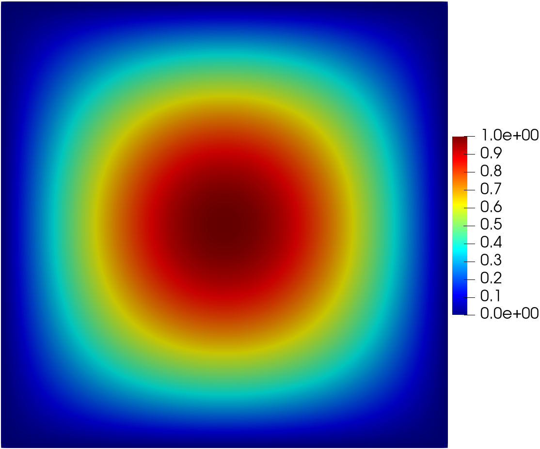
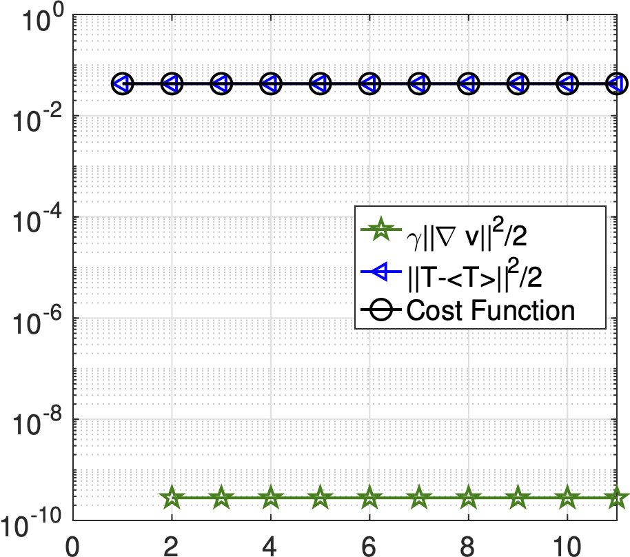
Figure 1: Example 5.12: Plots of temperature $T_{h}$ of $\kappa=1.0$ and $\gamma=1.0$ for (a). Optimal heat distribution $T_{h}^{9}$; and (b). Convergence profiles for cost functional.

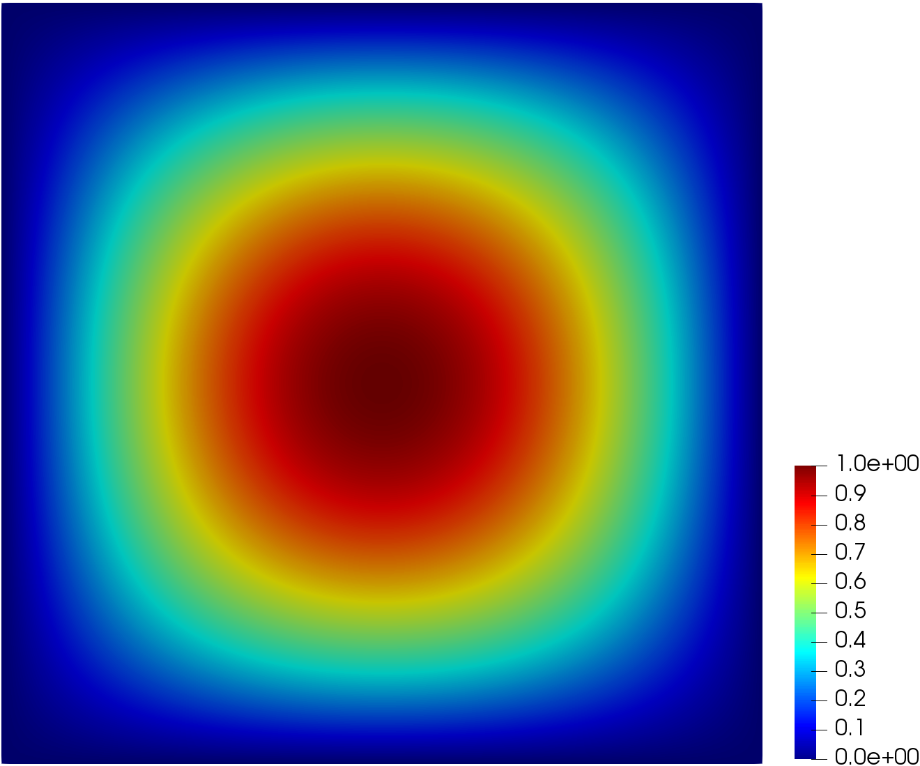
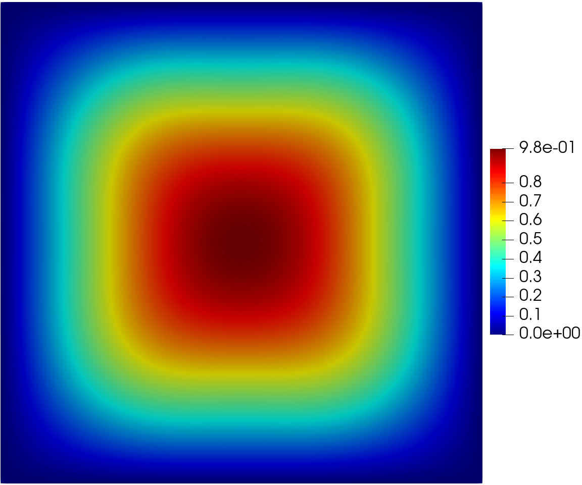
(a)	(b)
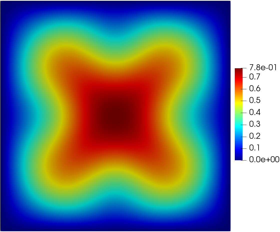
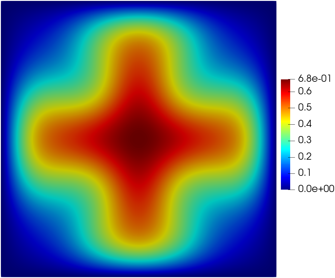
(c)	(d)

Figure 2: Example 5.12: Plots of temperature $T_{h}$ of $\kappa=1.0$ for (a). Initial heat distribution $T_{h}^{0}$; and with (b). $\gamma=3.6$E-6; (c). $\gamma=8.5$E-7; (d). $\gamma=3.9$E-7.

The initial heat distribution $T_{h}^{0}$ corresponding to $\mathbf{v}=0$ is shown in Fig. 2a. The optimal heat distribution $T_{h}$ corresponding to $\gamma=3.6$E-6, 8.5E-7, and 3.9E-7 are plotted in Fig. 2b-d. For the initial heat distribution, one can observe that the maximum of $T_{h}^{0}$ is 1.0. Thanks to advection effect, the “hot” region, which is at the center of the domain initially, is now spread out, but still inherits certain symmetric pattern. As a result, the heat distribution over the entire domain is evened out. Note that the maximum of $T_{h}$ is reduced to 9.8E-1, 7.8E-1, and 6.8E-1 corresponding to $\gamma=3.6$E-6, 8.5E-7, and $3.9$E-7, respectively. Also, it is shown from these plots that the smaller value in $\gamma$ (which indicates less penalty on the control), the more effective is the convection-cooling.

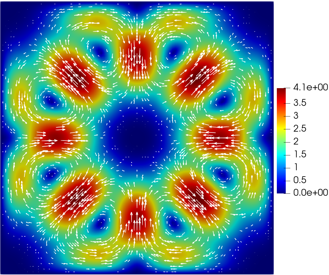
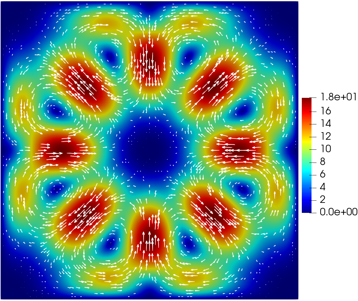
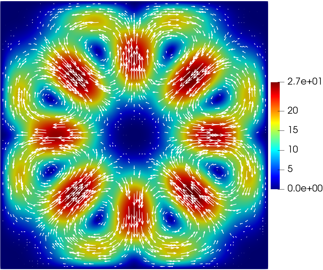
(a)	(b)	(c)

Figure 3: Example 5.12: Plots of velocity field ${\mathbf{v}}_{h}$ for $\kappa=1.0$ and (a). $\gamma=3.6$E-6; (b). $\gamma=8.5$E-7; (c). $\gamma=3.9$E-7. Here, the color illustrates the magnitude of velocity $\mathbf{v}_{h}$ and the vector plots the field of $\mathbf{v}_{h}$.

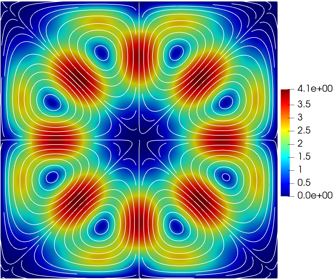
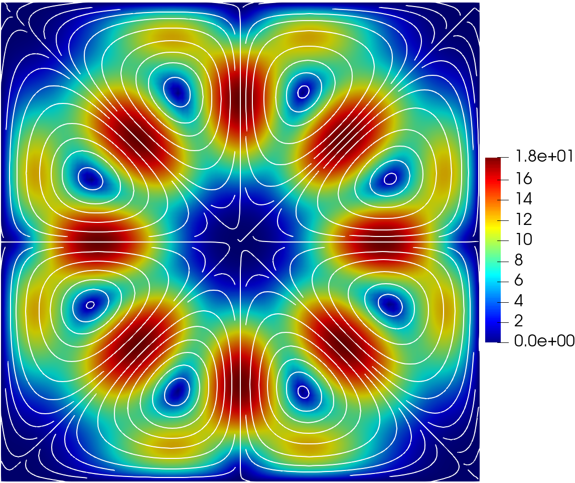
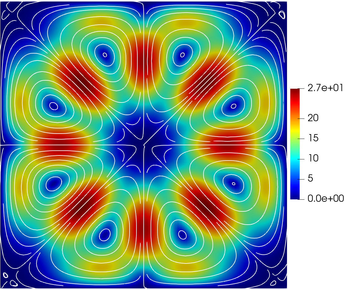
(a)	(b)	(c)

Figure 4: Example 5.12: Plots of streamlines of $\mathbf{v}_{h}$ for $\kappa=1.0$ and (a). $\gamma=3.6$E-6; (b). $\gamma=8.5$E-7; (c). $\gamma=3.9$E-7. Here, the color illustrates the magnitude of velocity $\mathbf{v}_{h}$ and the curve plots the streamline of $\mathbf{v}_{h}$.

On the other hand, as shown in Figs. 3-4, the optimal velocity fields $\mathbf{v}_{h}$ and their streamlines computed by our algorithm for different $\gamma$ well preserve the divergence-free condition and also present symmetric patterns. This also explains the symmetric pattern of the temperature distribution shown in Fig. 2. Moreover, the patterns for $\mathbf{v}_{h}$ are very similar for different $\gamma$ values. However, the magnitude of $\mathbf{v}_{h}$ increases as the $\gamma$ value decreases.

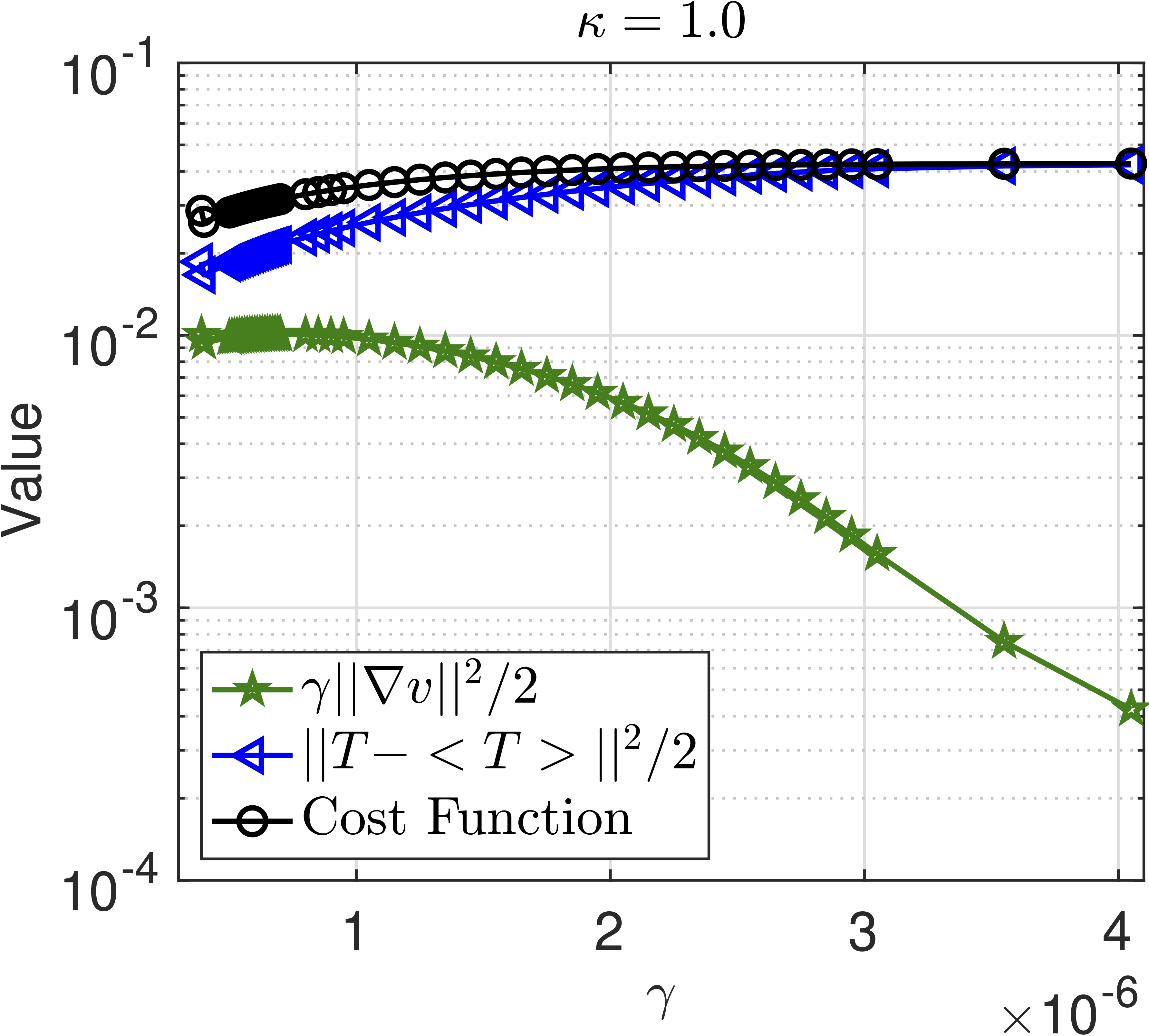
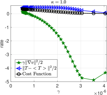
(a)	(b)

Figure 5: Example 5.12: Illustration of results for $\kappa=1.0$ (a). Plot of profiles in the cost functional with respect to $\gamma$ (here $\|T_{h}^{0}-\langle T_{h}^{0}\rangle\|^{2}/2=$4.287E-2); (b). Convergence rates $r_{J},r_{T}$ and $r_{\mathbf{v}}$ computed by (5.1)–(5.3)

.

Next, we investigate the behavior of the cost functional with respect to $\gamma\in$[3.9E-7,  4.1E-6]. In Fig. 5a, we plot the cost values versus various $\gamma$ values. It shows that smaller values in $\gamma$ lead to smaller cost functional values. When $\gamma=4$E-7, we obtain $J_{\min}=2.60$E-2, which is $39\%$ smaller than the initial value (which is $4.287$E-2). In Fig. 5b, we plot the convergence rates $r_{J},r_{T}$ and $r_{\mathbf{v}}$ computed by (5.1)–(5.3). In particular, it can be seen that the convergence rate $r_{J}$ gradually decreases from $0.35$ to almost $0$ as increasing the values in $\gamma$.

Remark 5.13.

We have tested different $\kappa$ and mesh sizes $h$ for Example 5.12 to demonstrate the numerical robustness, where different initial guesses for velocity are also tested. The numerical results are robust on $\kappa$ and refined $h$ for almost all $\gamma$ in the active region. To reduce the redundancy of the figures, they are omitted in the paper. However, the performance is slightly different when $\gamma$ is close to its lower limit. This is likely due to the fact that the continuous problem may fail to have the existence of an optimal control when $\gamma=0$. In this case, the cost functional loses its coercivity in the control input.

Example 5.14.

In this example, we consider an asymmetric distribution of the hear source. Let

$$f(x,y)=1000((x-0.5)^{2}+(y-0.75)^{2})x(1-x)y(1-y).$$

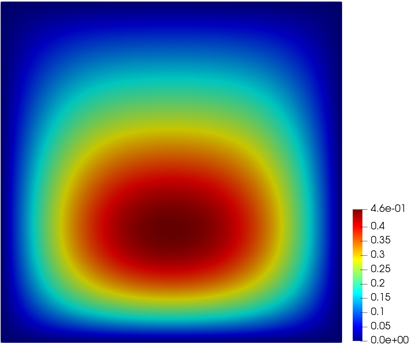
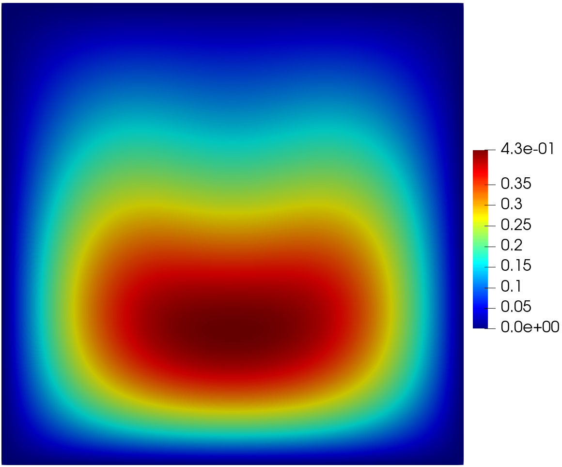
(a)	(b)
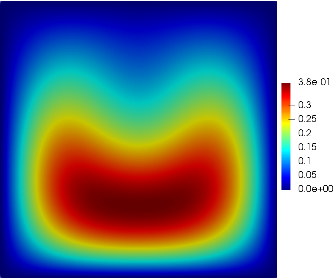
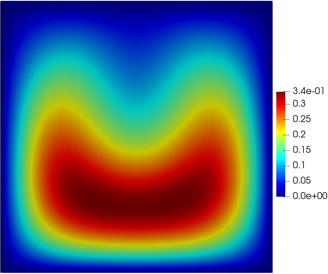
(c)	(d)

Figure 6: Example 5.14: Plots of optimal $T_{h}$ for $\kappa=1.0$ and (a). Initial heat distribution $T_{h}^{0}$; (b). $\gamma=1.8$E-6; (c). $\gamma=8$E-7; (d). $\gamma=4$E-7.

The initial heat distribution corresponding to $\gamma=1.0$ and $\mathbf{v}=0$ is plotted in Fig. 6a. As shown in this figure, the maximum of $T_{h}^{0}$ is 4.6E-1. The optimal heat distributions corresponding various values in $\gamma$ are plotted in Fig. 6b-c. We observe similar results as in Example 5.12, i.e., the smaller value in $\gamma$ will yield the lower maximum of the optimal temperature.

The optimal vector fields and their streamlines are demonstrated in Fig. 7-8. The profiles of the cost functional are plotted in Fig. 9. For $\gamma=4$E-7, we obtain the cost functional value $J_{\min}$ = 6.76E-3, which is 25% smaller than the initial value (which is $8.97$E-3). In this case, we observe that the convergence rate $r_{J}$ gradually decreases from $0.22$ to almost $0$.

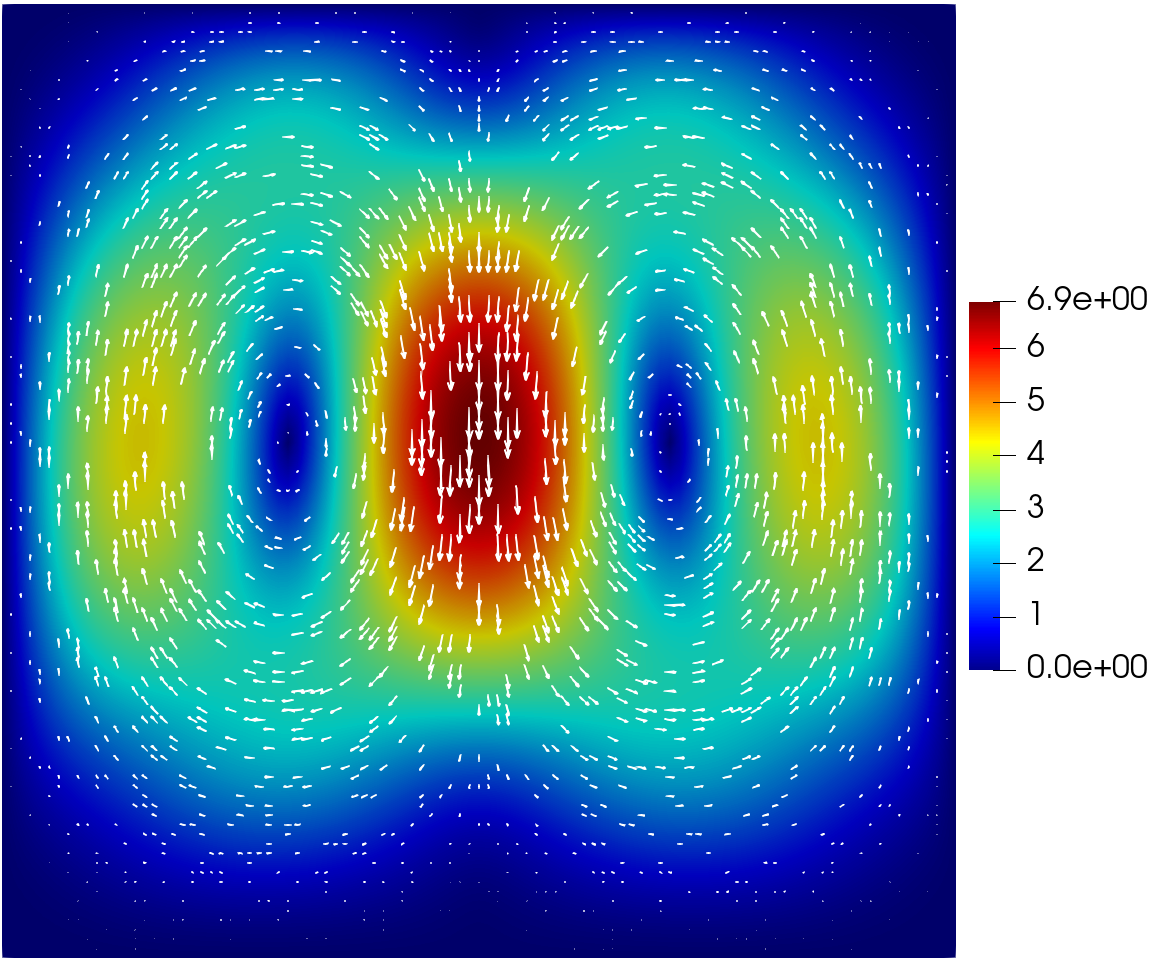
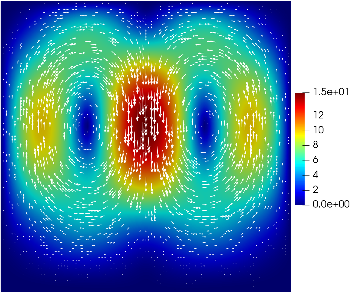
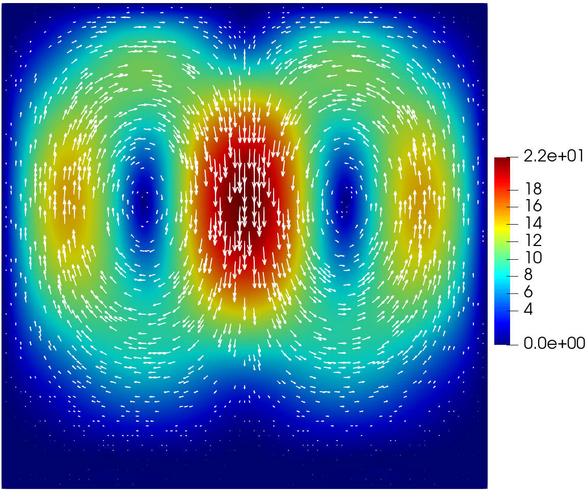
(a)	(b)	(c)

Figure 7: Example 5.14: Plots of temperature $T_{h}$ and vector field ${\mathbf{v}}$ for $\kappa=1.0$ and (a) $\gamma=1.8$E-6; (b)$\gamma=8$E-7; (c). $\gamma=4$E-7. Here, the color illustrates the magnitude of velocity $\mathbf{v}_{h}$ and the vector plots the field of $\mathbf{v}_{h}$.

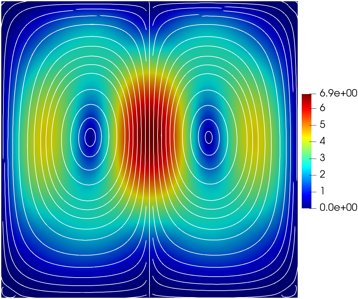
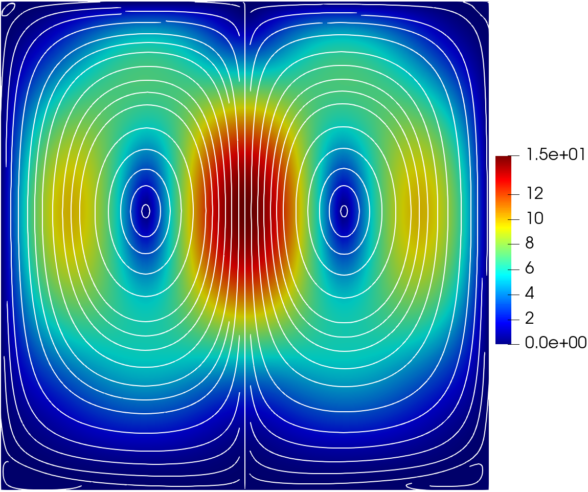
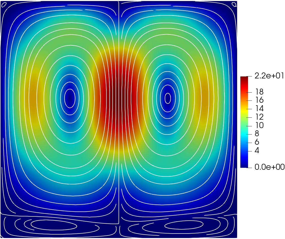
(a)	(b)	(c)

Figure 8: Example 5.14: Plots of temperature $T_{h}$ and vector field ${\mathbf{v}}$ for $\kappa=1.0$ and (a) $\gamma=1.8$E-6; (b)$\gamma=8$E-7; (c). $\gamma=4$E-7. Here, the color illustrates the magnitude of velocity $\mathbf{v}_{h}$ and the curve plots the streamline of $\mathbf{v}_{h}$.

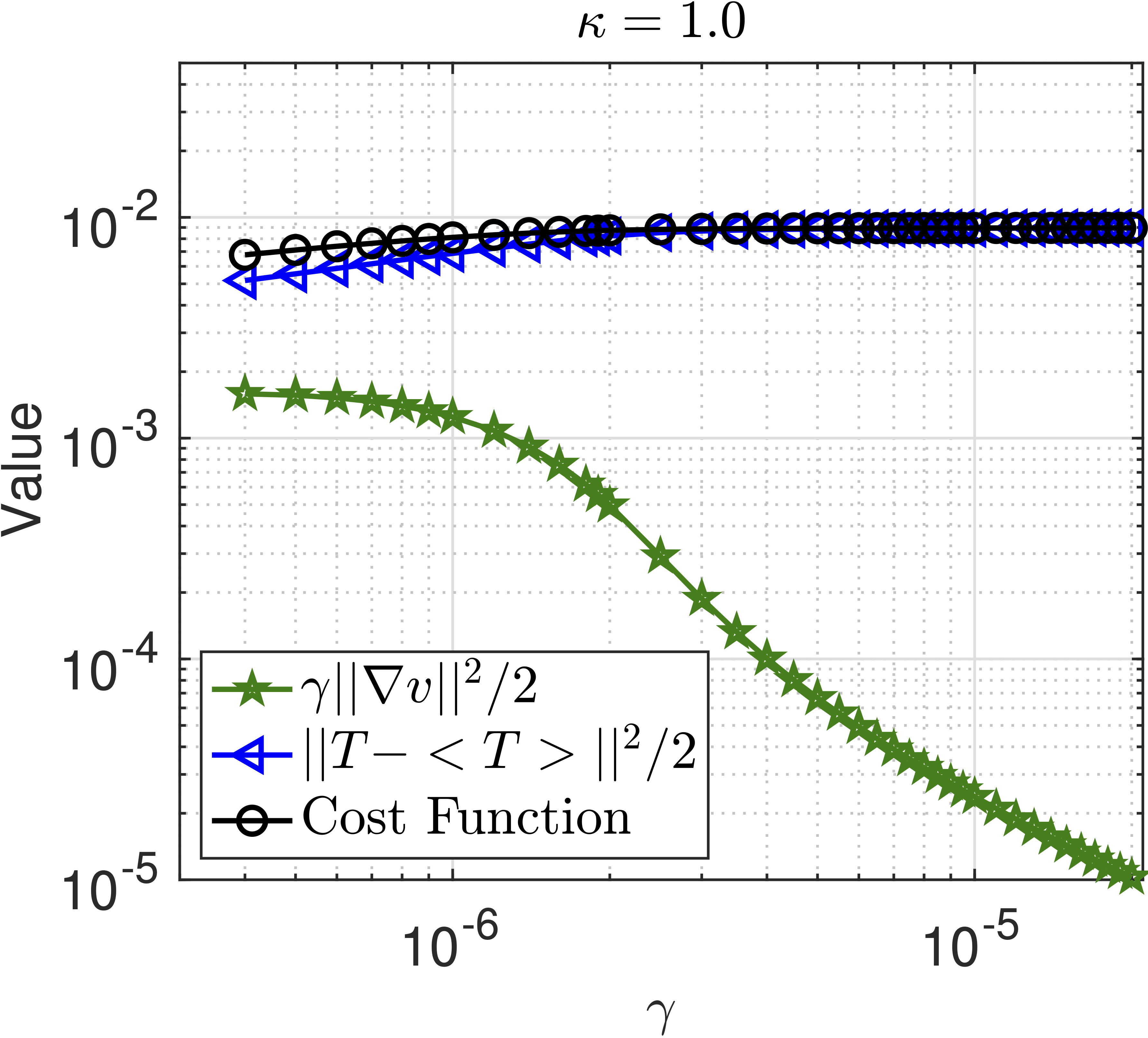
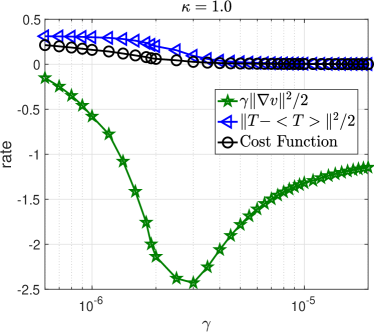
(a)	(b)

Figure 9: Example 5.14: Illustration of results for $\kappa=1.0$: (a). Plots of profiles in the cost functional with respect to $\gamma$ (here $\|T_{h}^{0}-\langle T_{h}^{0}\rangle\|^{2}/2=8.97$E-3); (b). Convergence rates $r_{J},r_{T}$ and $r_{\mathbf{v}}$ computed by (5.1)–(5.3)

.

Example 5.15.

In this example, we continue to examine an asymmetric distribution of the heat source, where the heat source is centered at the upper right corner. We especially examine the behavior of the velocity field subject to such a heat distribution with a sharp peak. Let

$$f(x,y)=100\exp(-100(x-0.75)^{2}-100(y-0.75)^{2}).$$

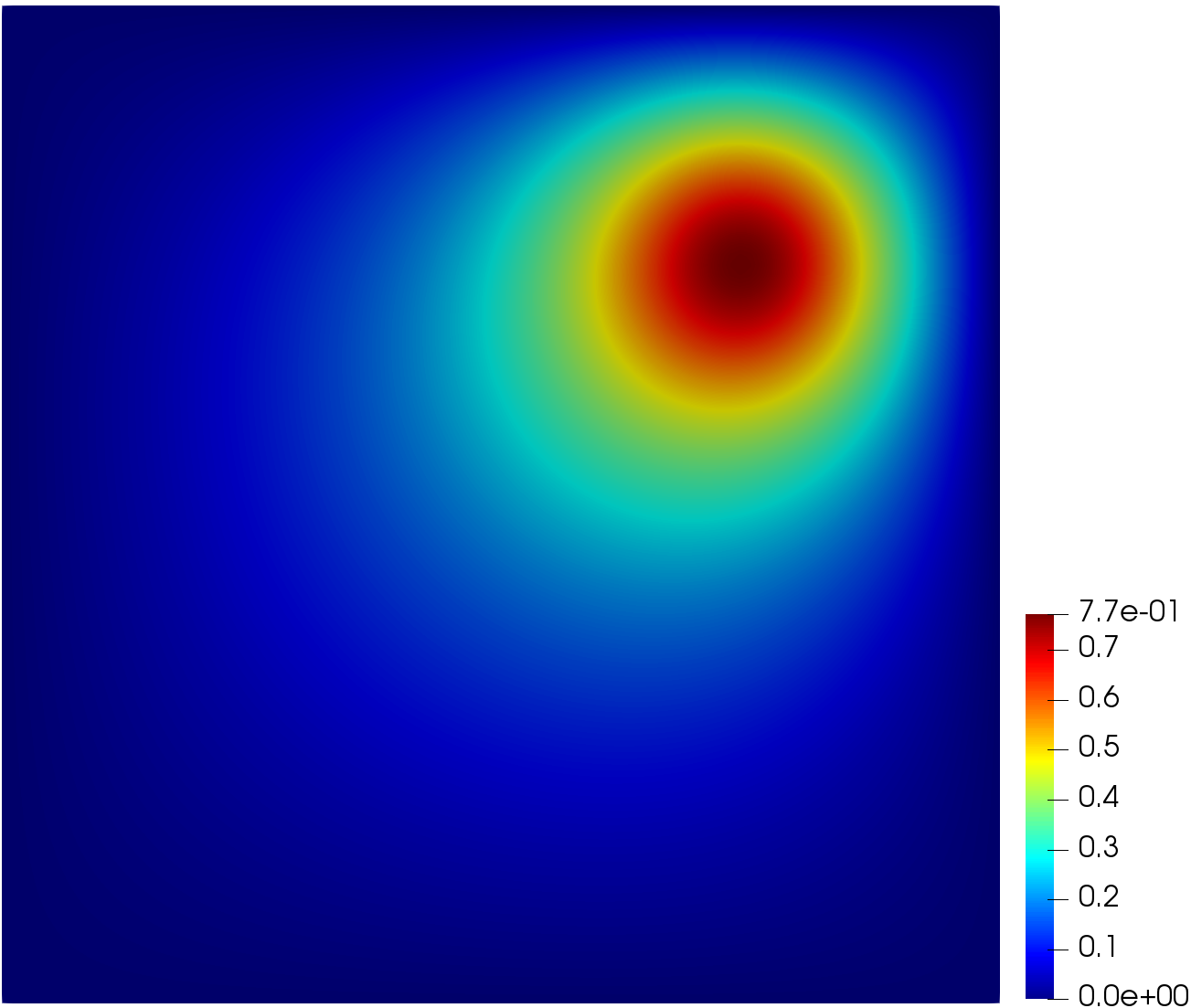
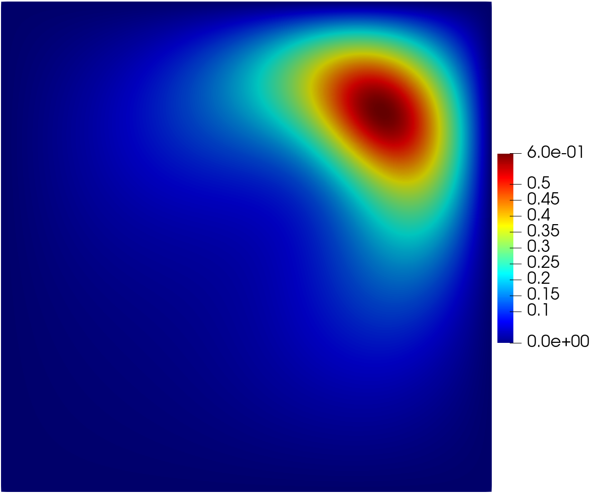
(a)	(b)
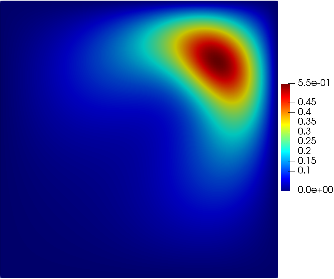
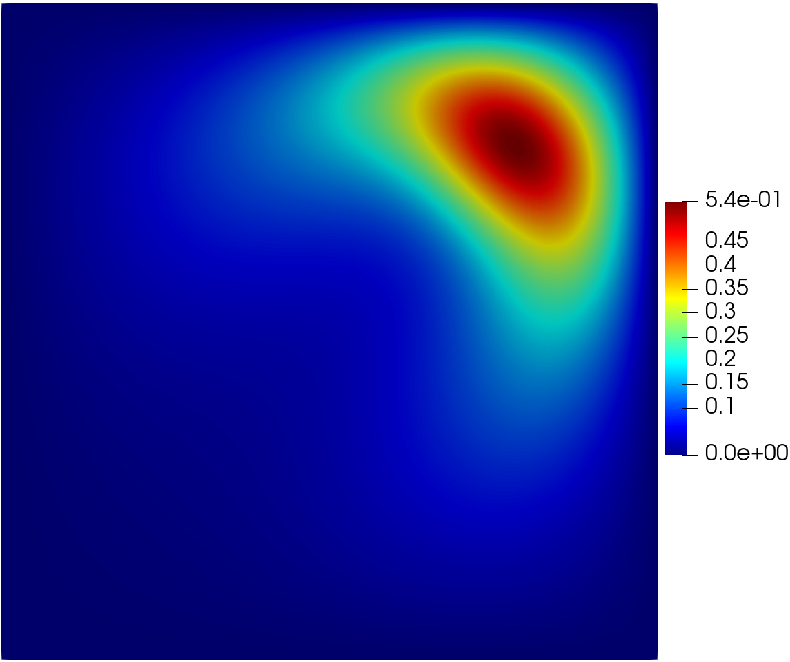
(c)	(D)

Figure 10: Example 5.15: Plots of optimal $T_{h}$ with $\kappa=1.0$ of (a). Initial heat distribution $T_{h}^{0}$; and (b). $\gamma=6$E-7; (c). $\gamma=3.7$E-7; (d). $\gamma=3.3$E-7.

The initial heat distribution corresponding to $\gamma=1.0$ and $\mathbf{v}=0$ is plotted in Fig. 10a. As shown in this figure, the maximum of $T_{h}^{0}$ is 7.7E-1. The numerical optimal solutions for heat distribution $T_{h}$ are plotted in Fig. 10 for $\gamma=$6E-7, 3.7E-8, and 3.3E-8. As we can observe in Fig. 13a, the maximum value of the heat distribution is reduced from $\max T_{h}^{0}=0.77$ to $\max T_{h}=0.6$, $\max T_{h}=0.55$, and $\max T_{h}=0.54$ corresponding to $\gamma$ =6E-7, 3.7E-7, and 3.3E-7, respectively. Similar to former examples, smaller value in $\gamma$ indicates a more effective cooling process.

Fig. 11-12 illustrate the velocity fields and the corresponding streamlines. Based on the direction fields we observe that for each case the velocity tends to “blow” the heat source further to the upper right corner, however due to divergence-free, the heat distribution is stretched toward to the cooler region. For this example, the velocity fields associated with different values of $\gamma$ also share a similar pattern. The profiles of the cost functional are plotted in Fig. 13. For $\gamma$ = 3.3E-7, we obtain the cost function value $J_{\min}$ = 7.74E-3, which is 38% smaller than the initial value (1.24E-2). In this case, we find that the convergence rate $r_{J}$ gradually decreases from $0.29$ to almost $0$.

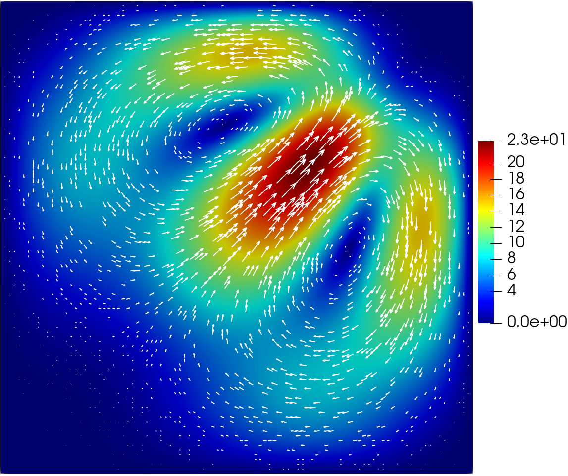
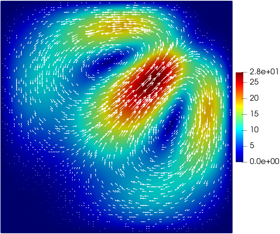
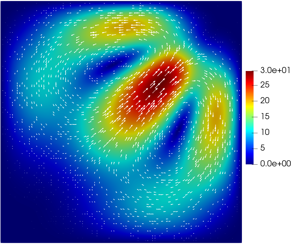
(a)	(b)	(c)

Figure 11: Example 5.15: Plots of optimal $\mathbf{v}_{h}$ for $\kappa=1.0$ and (a). $\gamma=6$E-7; (b). $\gamma=3.7$E-7; (c). $\gamma=3.3$E-7. Here, the color illustrates the magnitude of velocity $\mathbf{v}_{h}$ and the vector plots the field of $\mathbf{v}_{h}$.

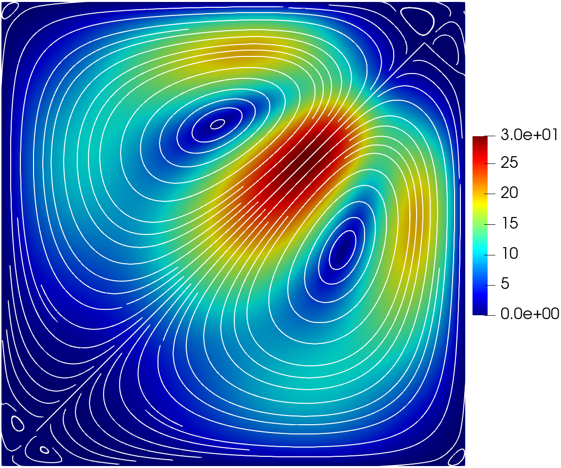
(a)	(b)	(c)

Figure 12: Example 5.15: Plots of optimal $T_{h}$ for $\kappa=1.0$ and (a). $\gamma=6$E-7; (b). $\gamma=3.7$E-7; (c). $\gamma=3.3$E-7. Here, the color illustrates the magnitude of velocity $\mathbf{v}_{h}$ and the curve plots the streamline of $\mathbf{v}_{h}$.

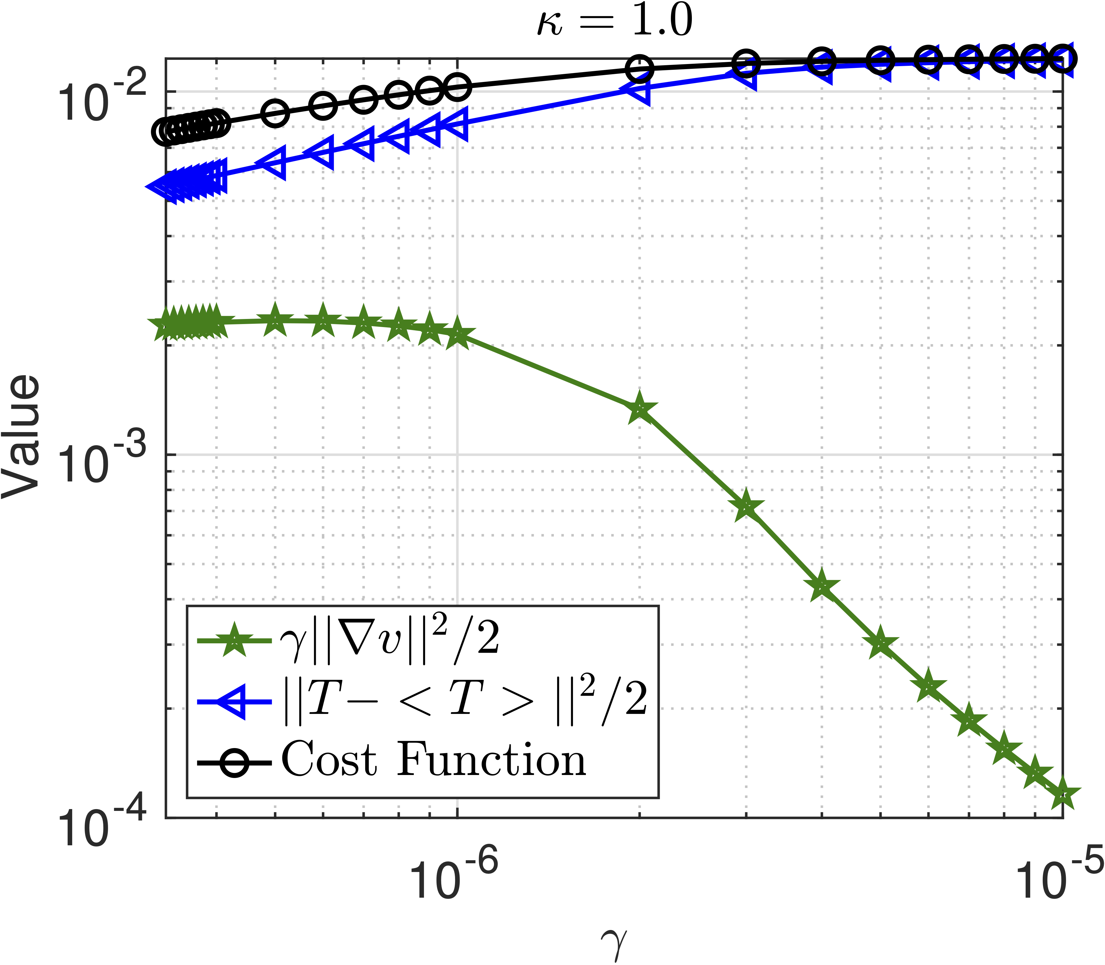
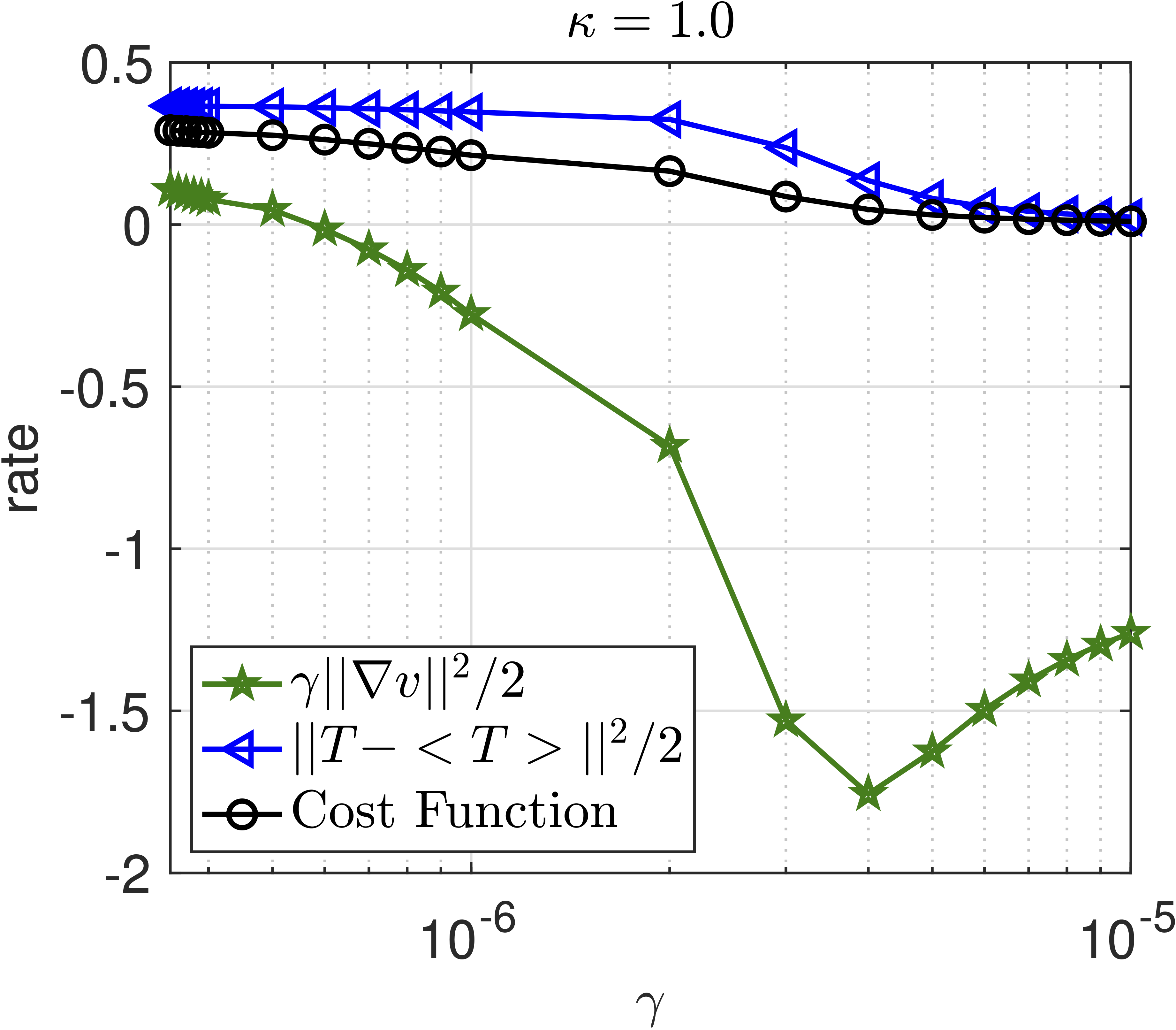
(a)	(b)

Figure 13: Example 5.15: Illustration of results for $\kappa=1.0$ (a). Plot of initial temperature $T_{h}^{0}$ (here $\|T_{h}^{0}-\langle T_{h}^{0}\rangle\|^{2}/2=1.24$E-2); (b) Plot of profiles in the cost functional with respect to $\gamma$; (c) Convergence rates $r_{J},r_{T}$ and $r_{\mathbf{v}}$ computed by (5.1)–(5.3)

.

Example 5.16.

In the last example, we consider that there is a heat source as well as a heat sink and examine how the velocity behaves in an environment with such heat distributions. Let

$$f(x,y)=75\exp(-(9x-2)^{2}/4-(9y-2)^{2}/4)-75\exp(-(9x-4)^{2}/4-(9y-7)^{2}/4).$$

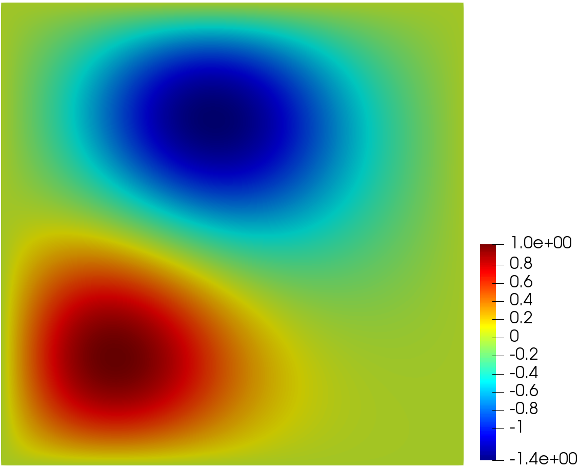
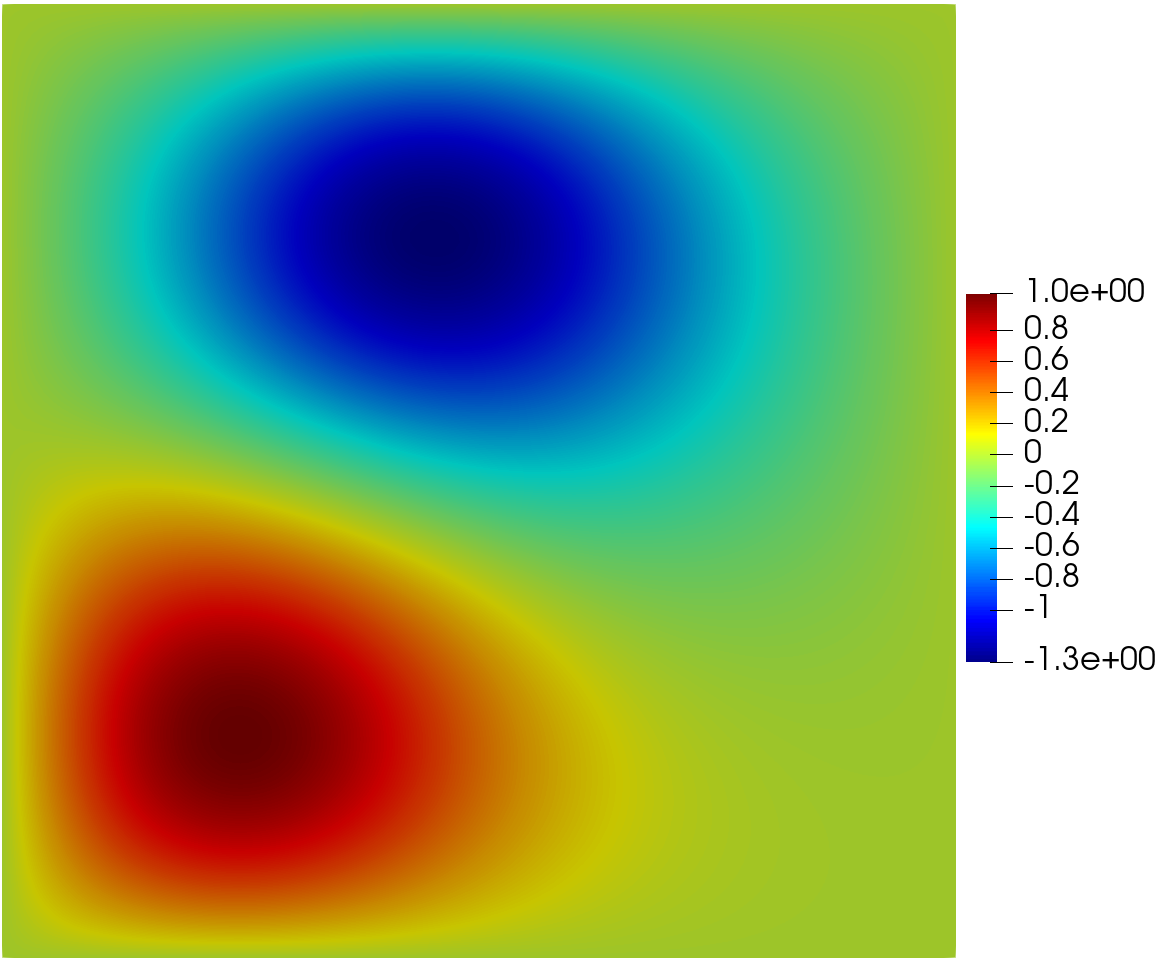
(a)	(b)
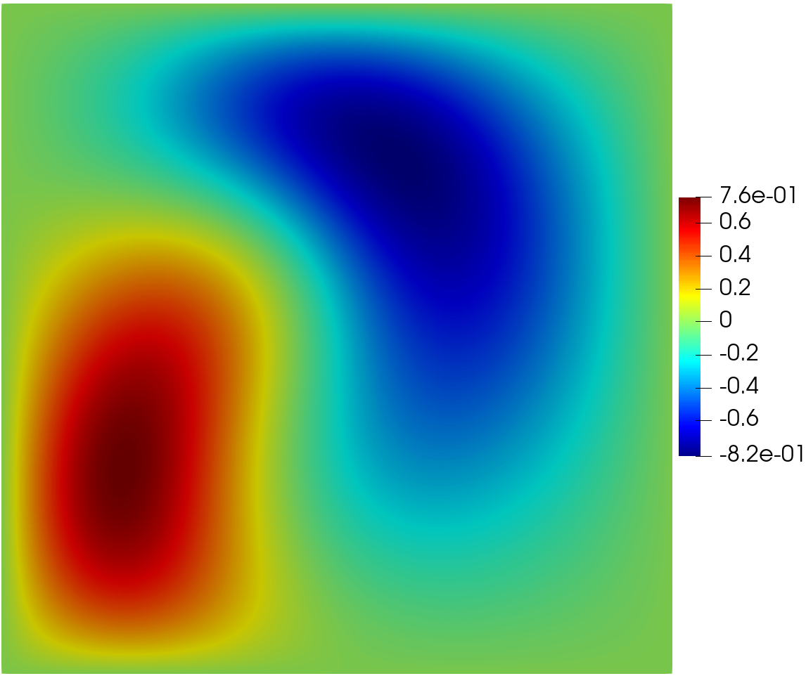
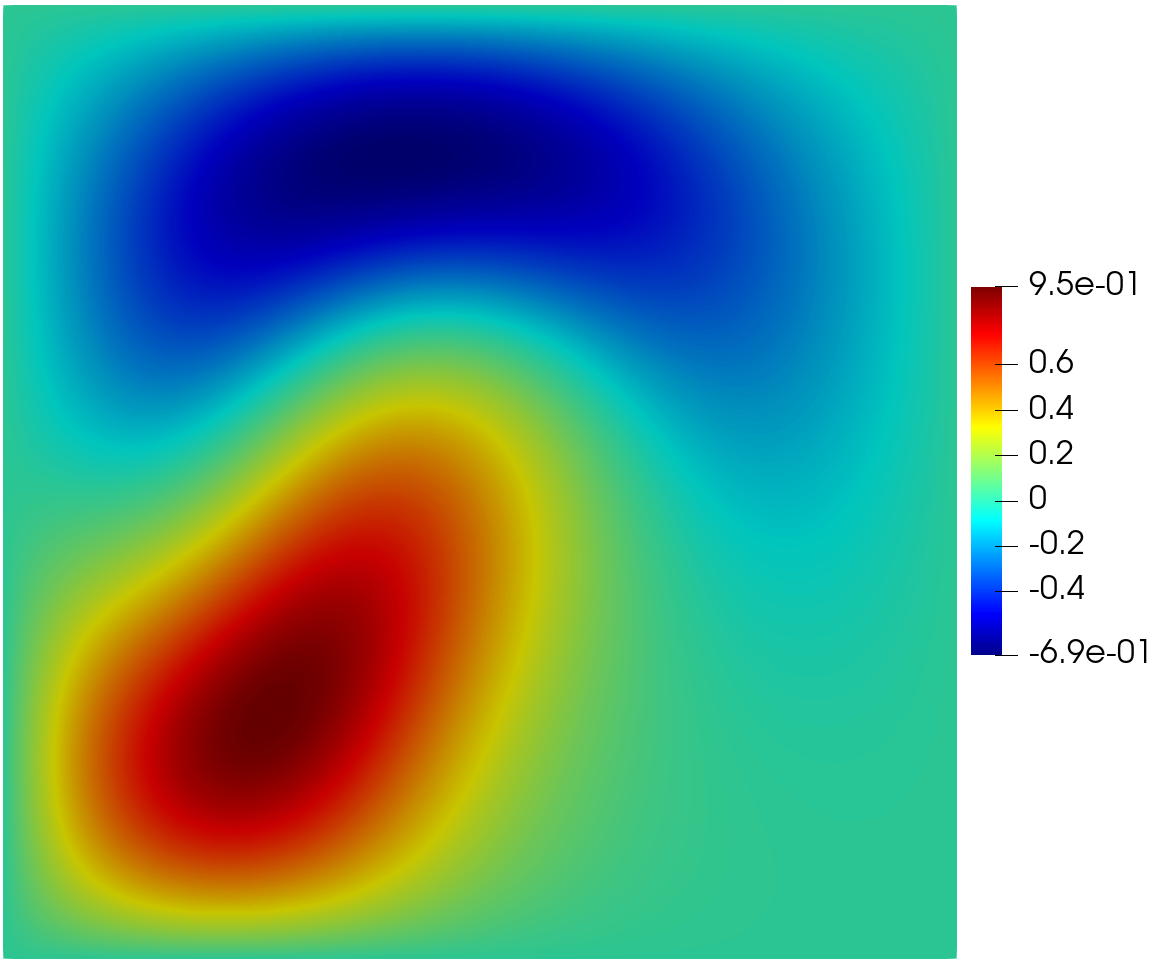
(c)	(d)

Figure 14: Example 5.16: Plots of optimal $T_{h}$ for $\kappa=1.0$ of (a). Initial heat distribution $T_{h}^{0}$; and (b). $\gamma=5$E-5; (c). $\gamma=1$E-5; (d). $\gamma=6.9$E-6 .

The initial heat distribution corresponding to $\gamma=1.0$ and $\mathbf{v}=0$ is plotted in Fig. 14a. As shown in this figure, the maximum and minimum values of of $T_{h}^{0}$ are $1.0$ and $-1.4$, respectively. The numerical optimal solutions for heat distribution $T_{h}$ are plotted in Fig. 14b-d for $\gamma=$5E-5, 1E-5, and 6.9E-6. We observe that the upper and lower bounds of the initial temperate are reduced from $T_{\min}=-1.4$ and $T_{\text{max}}=1$ (shown in Fig. 17a) to $(\min T_{h}=-1.3,\max T_{h}=1.0)$, $(\min T_{h}=-0.82,\max T_{h}=0.76)$, and $(\min T_{h}=-0.69,\max T_{h}=0.95)$ with respective to $\gamma$ =5E-5, 1E-5, and 6.9E-6. Different to former examples, it is shown in Fig. 15-16 that the velocity profiles differ significantly for these three values of $\gamma$. When $\gamma=$5E-5, as we can see in Figs. 16-15a, the velocity field seems to steer the cold region toward the hot region and thus the minimum value is increased from $-1.4$ to $-1.3$, however the maximum value remains at $1$. When $\gamma$ = 1E-5, as shown in Figs. 16-15a, it seems that the cold and the hot regions are advected simultaneously, and hence both the maximum and minimum values are tuned. However, as one further reduces the value in $\gamma$ from 5E-5 to 6.9E-6, the circulation between the cold and hot regions becomes disproportional, which results in a smaller minimum value of the temperature but a higher maximum compared to the case with $\gamma$=5E-5. This may be due to the disproportional steering effect of the velocity field shown in Figs. 15-16.

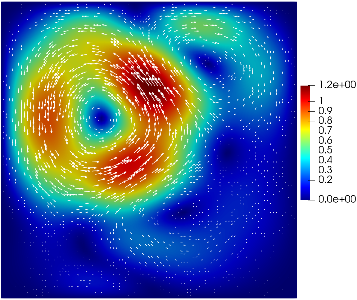
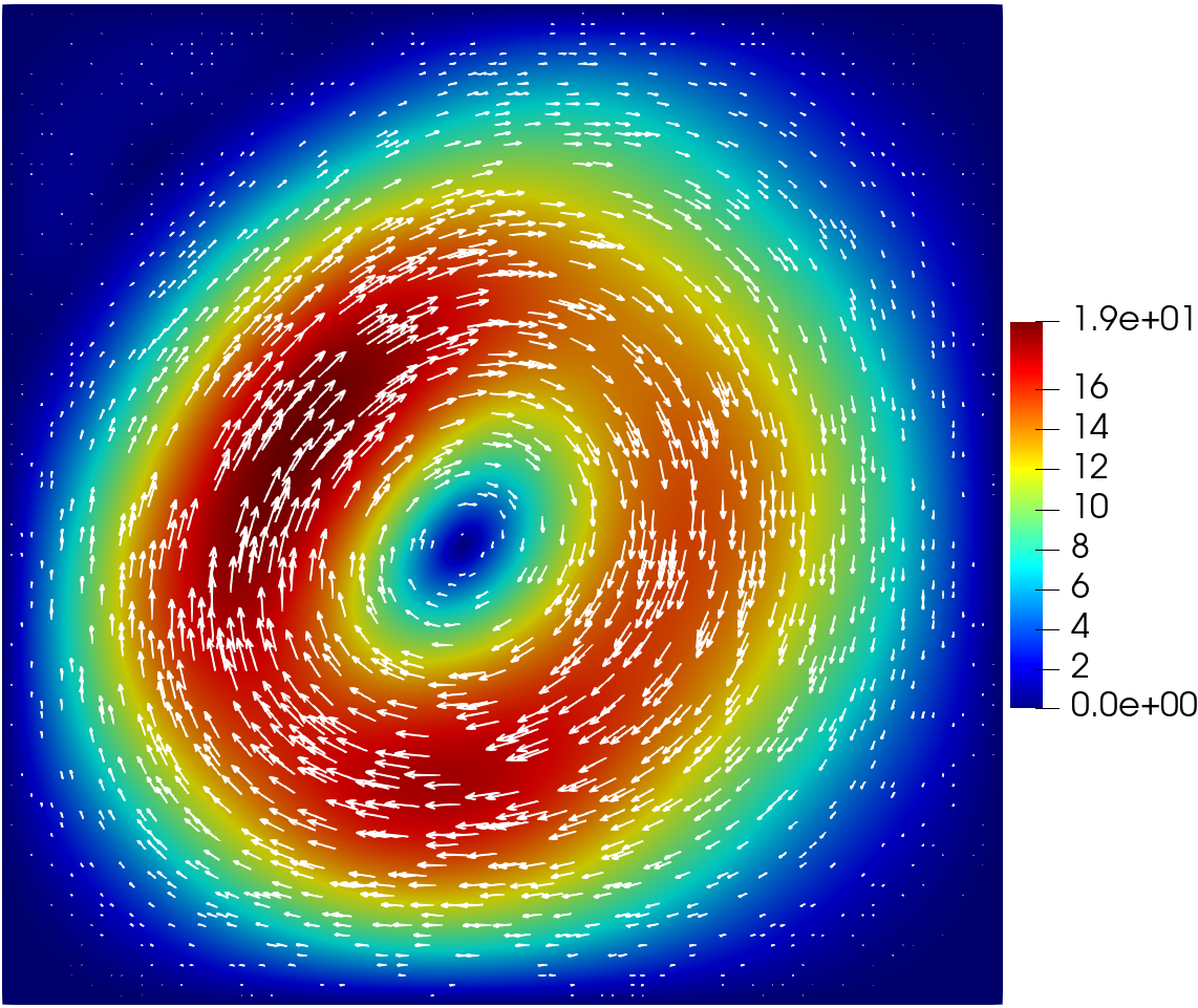
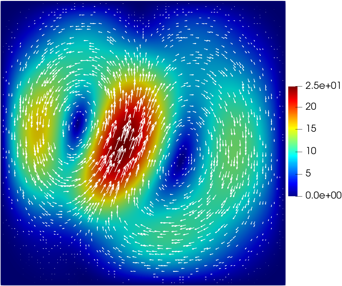
(a)	(b)	(c)

Figure 15: Example 5.16: Plots of optimal $\mathbf{v}_{h}$ for $\kappa=1.0$ and (a). $\gamma=5$E-5; (b). $\gamma=1$E-5; (c). $\gamma=6.9$E-6. Here, the color illustrates the magnitude of velocity $\mathbf{v}_{h}$ and the vector plots the field of $\mathbf{v}_{h}$.

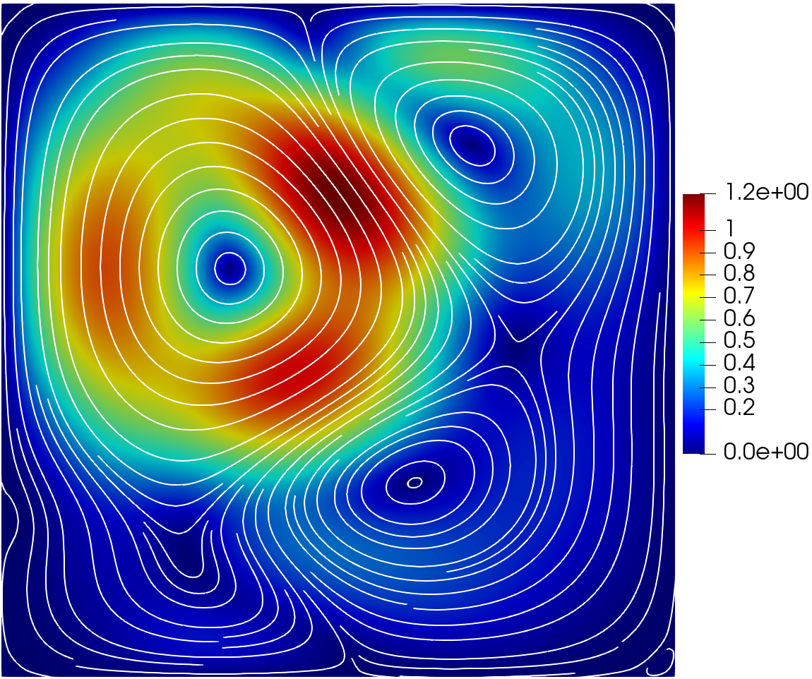
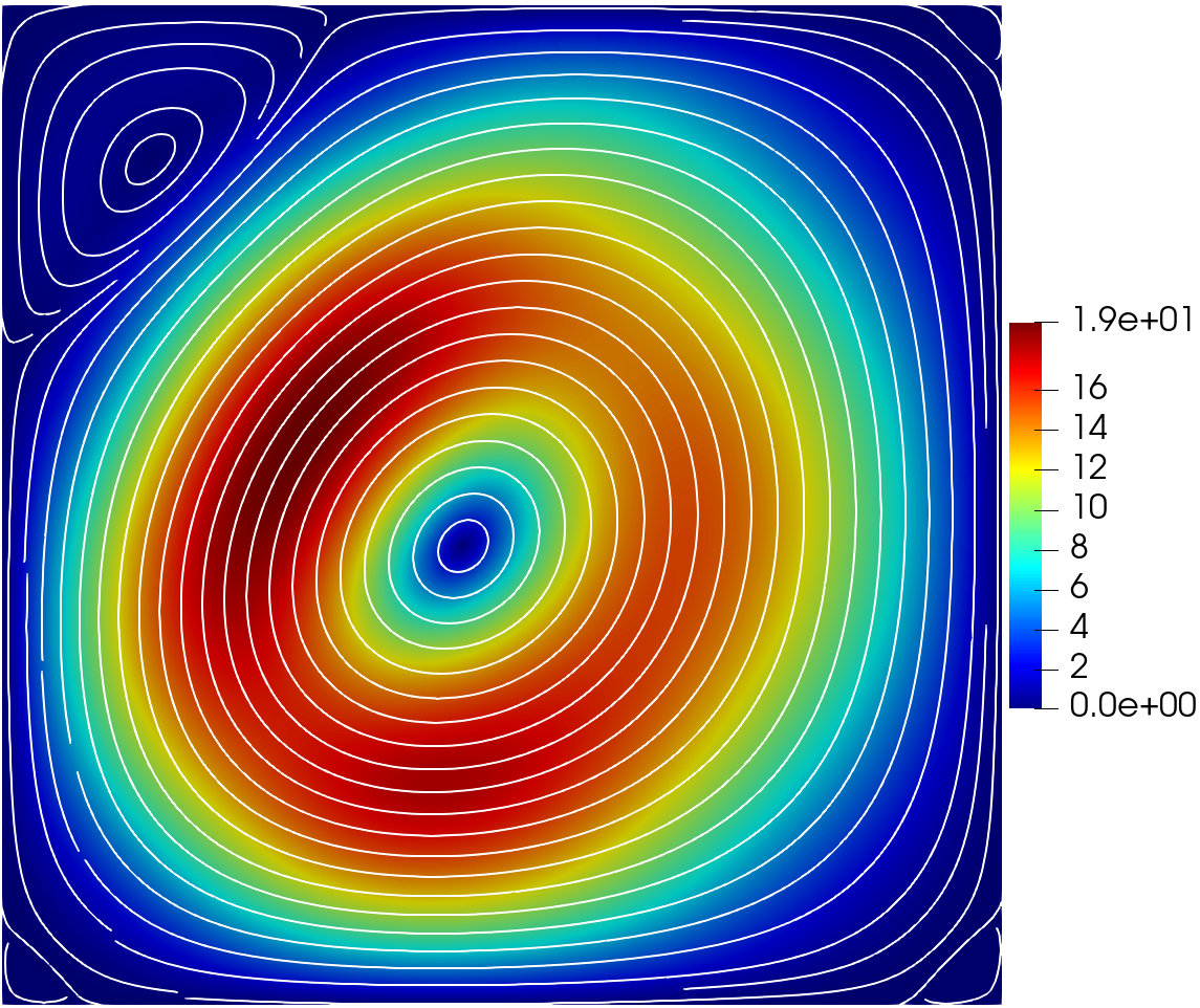
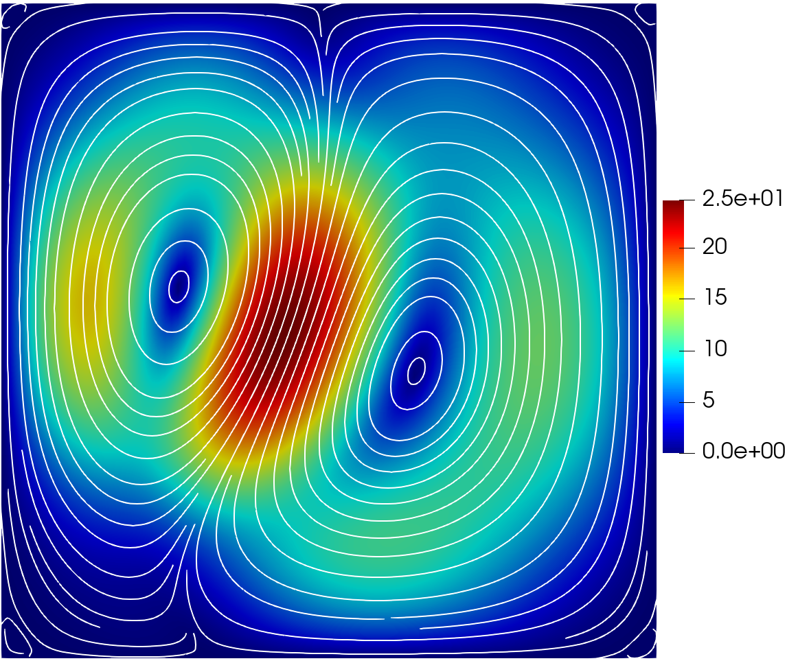
(a)	(b)	(c)

Figure 16: Example 5.16: Plots of optimal $\mathbf{v}_{h}$ for $\kappa=1.0$ and (a). $\gamma=5$E-5; (b). $\gamma=1$E-5; (c). $\gamma=6.9$E-6. Here, the color illustrates the magnitude of velocity $\mathbf{v}_{h}$ and the curve plots the streamline of $\mathbf{v}_{h}$.

Lastly, the convergence results are plotted in Fig. 17. Similar results as in the previous tests can be observed from these two figures. For $\gamma=$6.9E-6, the cost function $J_{\min}=$9.17E-2, which is $29\%$ smaller than the initial value (1.29E-1). In this case, we observe that the convergence rate $r_{J}$ gradually decreases from $0.31$ to almost $0$.

In summary, we have conducted a wide range of tests with differential values of $\gamma$ for different heat source distributions in this section. The numerical results demonstrate that using the optimal convection strategy, the cost functional value can be reduced by 25%-40% depending upon the source terms, when $\gamma\in$ [E-5, E-7].

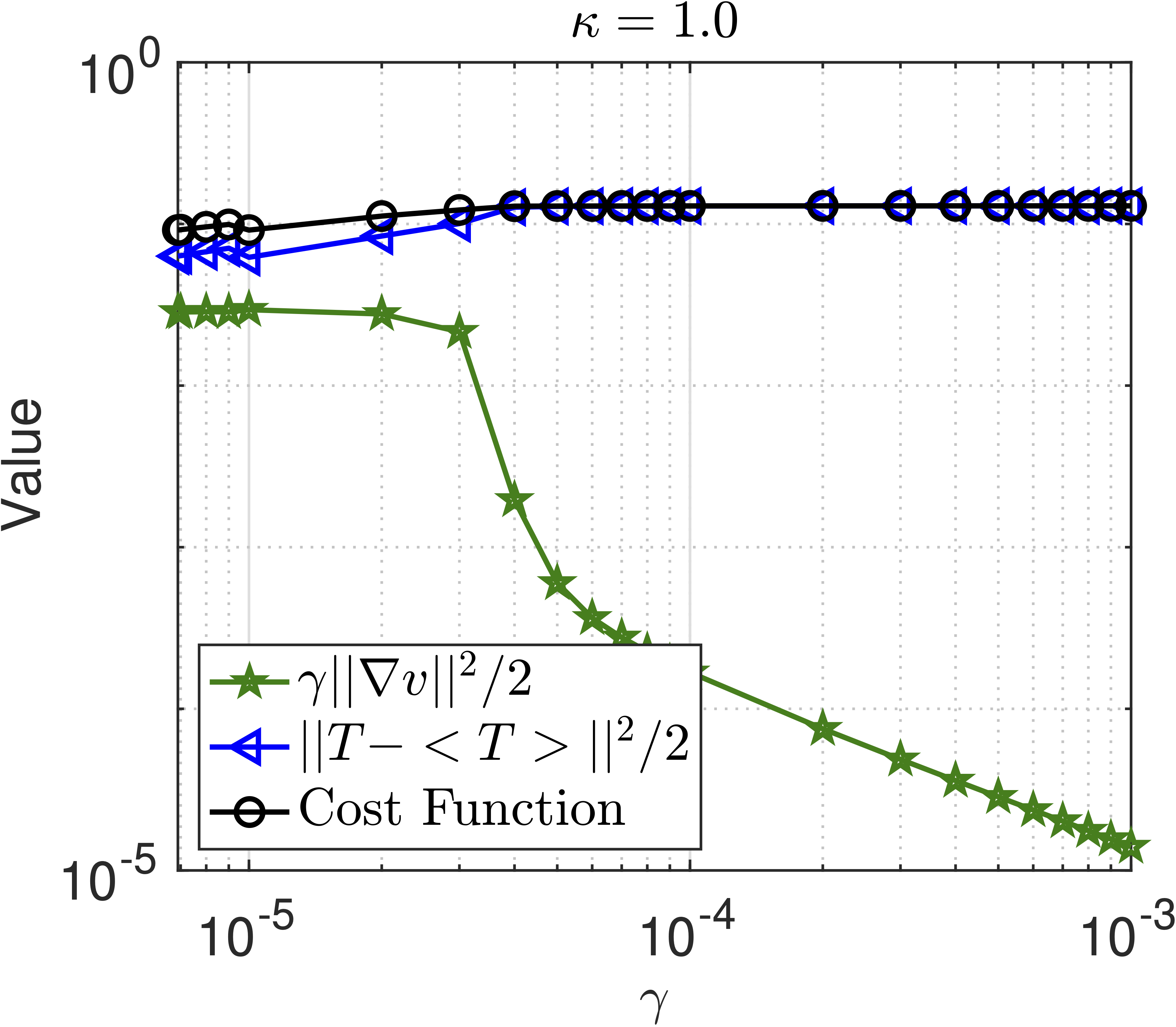
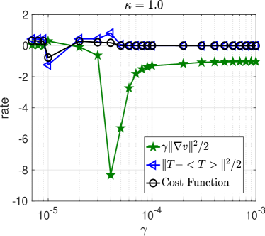
(a)	(b)

Figure 17: Example 5.16: Illustration of results for $\kappa=1.0$ (a). Plot of profiles in the cost functional with respect to $\gamma$ (here $\|T_{h}^{0}-\langle T_{h}^{0}\rangle\|^{2}/2=1.29$E-1); (b). Convergence rates $r_{J},r_{T}$ and $r_{\mathbf{v}}$ computed by (5.1)–(5.3)

.

6 Conclusion

In this paper, we discussed the optimal control design for convection-cooling via an incompressible velocity field. We presented rigorous theoretical analysis and conditions for solving and characterizing the optimal controller. Our numerical experiments demonstrate the effectiveness of the cooling process through flow advection. Moreover, we observed that to enhance heat transfer, small values in $\gamma$ may be employed in the convection-cooling design. We shall continue to address the convergence issues of our current numerical schemes applied to such nonlinear optimality systems. We shall also extend our results to study the non-stationary convection-cooling problems for more physical systems. Specifically, we shall consider to incorporate the flow dynamics into the velocity field, which will be controlled in real-time. How to construct effective numerical schemes to tackle such problems will be further investigated in our future work.

7 Acknowledgments

The authors sincerely thank the anonymous referees for their valuable comments and constructive suggestions. W. Hu was partially supported by the NSF grant DMS-1813570.

References

- [1] V. Barbu and G. Marinoschi, An optimal control approach to the optical flow problem, Systems & Control Letters, 87, pp. 1–9, 2016.
- [2] A. Bejan, Convection heat transfer, 2013. John wiley & sons.
- [3] T. L. Bergman, F. P. Incropera, A. S. Lavine, and D. P. DeWitt, Introduction to heat transfer, 2011. John Wiley & Sons.
- [4] J. A. Burns and E. M. Cliff, Numerical methods for optimal control of heat exchangers. in Proceedings 2014 American Control Conference, pp. 1649–1654, 2014.
- [5] J. A. Burns and B. Kramer, Full flux models for optimization and control of heat exchangers, in Proceedings of American Control Conference (ACC), pp.577–582, IEEE, 2015.
- [6] B. Calcagni, F. Marsili, and M. Paroncini, Natural convective heat transfer in square enclosures heated from below, Applied thermal engineering, 25(16), 2522–2531, 2005, Elsevier.
- [7] G. Chen, G. Fu, J. Singler and Y. Zhang, A Class of Embedded DG Methods for Dirichlet Boundary Control of Convection Diffusion PDEs, Journal of Scientific Computing, pp. 1–26, 2019.
- [8] G. Chen, J. Singler and Y. Zhang, An HDG method for Dirichlet boundary control of convection dominated diffusion PDEs, SIAM Journal on Numerical Analysis, 57(4), pp. 1919–1946, 2019.
- [9] G. Chen, W. Hu, J. Shen, J. Singler, Y. Zhang, and X. Zheng, An HDG method for distributed control of convection diffusion PDEs, Journal of Computational and Applied Mathematics, 343, pp. 643–661, 2018.
- [10] M. Corcione, Effects of the thermal boundary conditions at the sidewalls upon natural convection in rectangular enclosures heated from below and cooled from above, International Journal of Thermal Sciences, 42(2), 199–208, 2003.
- [11] A. Dalal and M. K. Das, Natural convection in a rectangular cavity heated from below and uniformly cooled from the top and both sides, Numerical Heat Transfer, Part A: Applications, 49(3), 301–322, 2006, Taylor & Francis.
- [12] L. Dede’ and A. Quarteroni, Optimal control and numerical adaptivity for advection–diffusion equations, ESAIM: Mathematical Modelling and Numerical Analysis, 39(5), pp. 1019–1040, 2005.
- [13] L. C. Evans, Partial Differential Equations, Vol. 19 of Graduate studies in mathematics, American Mathematical Soc., 2010.
- [14] C. Foias, O. Manley, R. Rosa, and R. Temam, Navier-Stokes equations and turbulence, vol. 83, 2001, Cambridge University Press.
- [15] W. Gong, W. Hu, M. Mateos, J. Singler, X. Zhang, and Y. Zhang, A new HDG method for Dirichlet boundary control of convection diffusion PDEs II: Low regularity, SIAM Journal on Numerical Analysis, 56(4), pp. 2262–2287, 2018.
- [16] W. Hu, Enhancement of heat transfer in stokes flows, Proceedings of the 56th IEEE Conference on Decision and Control, pp. 59–63, 2017.
- [17] W. Hu and O. San, Optimal Control of Heat Transfer in Unsteady Stokes Flows, 2018 IEEE Conference on Decision and Control (CDC), pp. 3752–3757, 2018.
- [18] W. Hu, J. Shen, J. Singler, Y. Zhang, and X. Zheng, A superconvergent HDG method for distributed control of convection diffusion PDEs, Journal of Scientific Computing, 76(3), pp. 1436–1457, 2018.
- [19] F. Kreith, R. M. Manglik, and M. S. Bohn, Principles of heat transfer, 2012. Cengage learning.
- [20] J.-L. Lions, Optimal control of systems governed by partial differential equations, Springer Verlag, 1971.
- [21] W. Liu, Mixing enhancement by optimal flow advection, SIAM journal on control and optimization, 47(2), 624–638, 2008.
- [22] I. Sezai and A. A. Mohamad, Natural convection in a rectangular cavity heated from below and cooled from top as well as the sides, Physics of Fluids, 12(2), 432–443, 2000, American Institute of Physics.
- [23] G. Stampacchia, Le problème de Dirichlet pour les équations elliptiques du second ordre à coefficients discontinus, Annales de l’institut Fourier, 15(1), 189–257, 1965.
- [24] R. Temam, Navier-Stokes Equations, Theory and Numerical Analysis, Studies in Mathematics and Its Applications, Vol. 2, North-Holland.
- [25] R. Temam, Infinite-dimensional dynamical systems in mechanics and physics, Vol. 68, 2012, Springer Science & Business Media.
- [26] X. Zhang, Y. Zhang, and J. Singler, An optimal EDG method for distributed control of convection diffusion PDEs, International Journal of Numerical Analysis and Modeling, 16 (4), pp. 519–542, 2019.
- [27] S. C. Brenner and L. R. Scott. The mathematical theory of finite element methods, volume 15 of Texts in Applied Mathematics. Springer-Verlag, New York, second edition.
- [28] F. Brezzi and R. Falk. Stability of higher order Taylor-Hood methods. SIAM J. Numer. Anal, 28(3):581–590, 1991
- [29] The FEniCS Project Version 1.5 M. S. Alnaes, J. Blechta, J. Hake, A. Johansson, B. Kehlet, A. Logg, C. Richardson, J. Ring, M. E. Rognes and G. N. Wells Archive of Numerical Software, vol. 3, 2015.