On the Various Extensions of the BMS Group

Romain Ruzziconi111e-mail: rruzzico@ulb.ac.be


Université Libre de Bruxelles and International Solvay Institutes
CP 231, B-1050 Brussels, Belgium
Thesis submitted in fulfilment of the requirements of
the PhD Degree in Sciences (“Docteur en Sciences”)

Academic year 2019-2020

Supervisor: Prof. Glenn Barnich

Thesis jury:

Prof. Riccardo Argurio (Université libre de Bruxelles)
Prof. Geoffrey Compère (Université libre de Bruxelles)
Prof. Daniel Grumiller (Technische Universität Wien)
Prof. Marios Petropoulos (École Polytechnique de Paris)

Abstract

The Bondi-Metzner-Sachs-van der Burg (BMS) group is the asymptotic symmetry group of radiating asymptotically flat spacetimes. It has recently received renewed interest in the context of the flat holography and the infrared structure of gravity. In this thesis, we investigate the consequences of considering extensions of the BMS group in four dimensions with superrotations. In particular, we apply the covariant phase space methods on a class of first order gauge theories that includes the Cartan formulation of general relativity and specify this analysis to gravity in asymptotically flat spacetime. Furthermore, we renormalize the symplectic structure at null infinity to obtain the generalized BMS charge algebra associated with smooth superrotations. We then study the vacuum structure of the gravitational field, which allows us to relate the so-called superboost transformations to the velocity kick/refraction memory effect. Afterward, we propose a new set of boundary conditions in asymptotically locally (A)dS spacetime that leads to a version of the BMS group in the presence of a non-vanishing cosmological constant, called the ΛΛ\Lambda-BMS asymptotic symmetry group. Using the holographic renormalization procedure and a diffeomorphism between Bondi and Fefferman-Graham gauges, we construct the phase space of ΛΛ\Lambda-BMS and show that it reduces to the one of the generalized BMS group in the flat limit.

Acknowledgements

This thesis could not have been completed without the help and support of several people. First, I am indebted to my supervisor, Glenn Barnich, for having guided my first steps in the marvellous world of asymptotic symmetries, from my Master’s studies to my PhD. I am grateful to him for having shared his extensive knowledge on the subject and his enthusiasm about research. He has been an example of rigour and independence that will definitely influence the future of my research. I would also like to thank him for the complete freedom that I had in my research, which allowed me to start new collaborations and complete side-projects.

Furthermore, I am grateful to Geoffrey Compère for the many projects and ideas he shared with me. I also thank him for his availability for discussions at all stages of the projects.

I would also like to thank Adrien Fiorucci for the numerous hours of stimulating discussions that were the origin of many of the original ideas presented in this thesis. Our collaboration and friendship are among the best memories I will keep from this PhD experience.

I thank my other collaborators, Luca Ciambelli, Pujian Mao, Charles Marteau, Marios Petropoulos, for a fruitful exchange of ideas. Collaborating with them was a real enlightenment.

I would like to thank Francesco Alessio, Laura Donnay, Daniel Grumiller, Yannick Herfray and Céline Zwikel for interesting discussions that will set the basis for future collaborations.

Moreover, I thank all the members of the Mathematical Physics research group for the nice and emulating atmosphere.

Once again, I would like to thank the members of my PhD jury Riccardo Argurio, Geoffrey Compère, Daniel Grumiller and Marios Petropoulos for agreeing to be my examiners and for their time dedicated to read this thesis.

From a personal perspective, I thank my family and friends for their support throughout the whole process.

This work was supported by the FRIA, F.R.S.-FNRS Belgium (2016-2020).

Chapter 1 Introduction

To specify most of the physical theories, one has to consider two ingredients: the kinematics which defines the allowed states and observables of the system, and the dynamics which dictates the evolution of the state through some equations of motion. An essential piece to define the kinematics is the set of boundary conditions that selects, using the equations of motion, the allowed solutions of the theory. Depending on the context, this set of boundary conditions should enable one to determine the exact initial conditions/characteristic initial value problem that one has to provide to select a particular solution in the allowed space. The choice of boundary conditions is dictated by the physical situation one wants to describe. As broadly illustrated in this thesis, several sets of boundary conditions may be relevant to specify the kinematics for the same dynamical part of the theory.

In this work, we are mainly interested by the study of boundary conditions in gauge theories, and especially in general relativity. Indeed, gauge theories are of major importance in physics since they are involved in the description of the four fundamental interactions through the standard model of particle physics and the general relativity theory. Furthermore, as their name suggests, gauge theories exhibit some symmetries of the dynamics called gauge symmetries. Among the gauge symmetries preserving the chosen boundary conditions, several will be trivial and seen as redundancies of the theory, while others will change the physical state of the system by their actions. The latter are called asymptotic symmetries and form a group (or, more generally, a groupoid) known as the asymptotic symmetry group. In particular, different sets of boundary conditions lead to different asymptotic symmetry groups.

In a series of seminal papers [1, 2, 3], Bondi, Metzner, Sachs and van der Burg have shown that the asymptotic symmetry group of four-dimensional general relativity in asymptotically flat spacetimes at null infinity is an infinite-dimensional group enhancing the Poincaré group and is called the (global) BMS group. It is given by the the semi-direct product between the Lorentz group and an infinite-dimensional enhancement of the translations, called the supertranslations. This result was very surprising since one could have naively expected to find the symmetry group of flat space by studying the behaviour of the gravitational field in asymptotic regions. However, this infinite-dimensional enhancement was necessary to allow for some radiative spacetime solutions. Furthermore, this analysis led to the Bondi mass loss formula, which states that the the flux of energy-momentum at null infinity is positive. This argument served to resolve the then-controversial debate of whether gravitational waves are physical or a pure gauge artifact of the linearized theory [4].

An extension of the global BMS algebra has recently been proposed, called the extended BMS algebra [5, 6, 7]. More precisely, the Lorentz part of the semi-direct sum defining the BMS algebra has been enhanced into the infinite-dimensional algebra of conformal transformations in two dimensions. These new symmetries are called superrotations (or super-Lorentz transformations [8]). At the level of the group, these superrotations are singular when considering the topology of the sphere as sections of null infinity. Therefore, only the global subgroup of the extended BMS group is globally well defined, which justifies the epithet “global”. As discussed in the following, this singular extension has been shown to be of major importance when considered as symmetries of the 𝒮𝒮\mathcal{S}-matrix of quantum gravity [9, 10, 11]. Even more recently, an alternative extension of the BMS group has been considered by replacing the singular superrotations with smooth Diff(S2)superscript𝑆2(S^{2}) superrotations [12, 13]. This new extension, called the generalized BMS group, is made possible by relaxing the definition of asymptotic flatness and allowing a fluctuating induced boundary metric.

It should be noted that the analysis of asymptotic symmetries in general relativity has been purused for other types of asymptotics and other spacetime dimensions, including three- and four-dimensional asymptotically anti-de Sitter (AdS) and asymptotically de Sitter (dS) spacetimes (see e.g. [14, 15, 16, 17, 18, 19]). Furthermore, it has been performed on other types of gauge theories including Maxwell, Yang-Mills and Chern-Simons theories (see e.g. [20, 21, 22, 23, 24, 25, 26]). The interests of these investigations are various and depend on the main research question. In section 1.1, following [27], we relate the study of asymptotic symmetries in gauge theories with major research directions in theoretical physics.

1.1 Use of asymptotic symmetries

The study of asymptotic symmetries in gauge theories is an old subject that has recently received renewed interest. A first direction is motivated by the AdS/CFT correspondence where the asymptotic symmetries of the gravity theory in the bulk spacetime correspond to the global symmetries of the dual quantum field theory through the holographic dictionary [28, 29, 30, 31, 32]. A strong control of asymptotic symmetries allows us to investigate new holographic dualities. A second direction is driven by the recently-established connections among asymptotic symmetries, soft theorems and memory effects [10]. These connections furnish crucial information about the infrared structure of quantized gauge theories. In gravity, they may be relevant to solve the long-standing problem of black hole information paradox [33, 34, 35, 36, 37].

1.1.1 Holography

The holographic principle states that quantum gravity can be described in terms of lower-dimensional dual quantum field theories [28, 29]. A concrete realization of the holographic principle asserts that the type IIB string theory living in the bulk spacetime AdS5 ×\times S5superscript𝑆5S^{5} is dual to the 𝒩=4𝒩4\mathcal{N}=4 supersymmetric Yang-Mills theory living on the four-dimensional spacetime boundary [30]. The gravitational theory is effectively living in the five-dimensional spacetime AdS5, the five dimensions of the factor S5superscript𝑆5S^{5} being compactified. A first extension of this original holographic duality is the AdS/CFT correspondence, which tells us that the gravitational theory living in the (d+1)𝑑1(d+1)-dimensional asymptotically AdS spacetime is dual to a CFT living on the d𝑑d-dimensional boundary. Other holographic dualities with different types of asymptotics have also been studied. A holographic dictionary enables one to interpret properties of the bulk theory in terms of the dual boundary theory. For example, the dictionary poses the following relationship between the symmetries of the two theories:

[Gauge symmetries in the bulk theoryGlobal symmetries in the boundary theory.]delimited-[]Gauge symmetries in the bulk theoryGlobal symmetries in the boundary theory\left[\begin{array}[]{c}\text{Gauge symmetries in the bulk theory}\\ \Longleftrightarrow\\ \text{Global symmetries in the boundary theory}.\end{array}\right] (1.1.1)

More specifically for us, consider a given bulk solution space with asymptotic symmetries. The correspondence tells us that a set of quantum field theories exist that are associated with the bulk solutions, such that in the UV regime, the global symmetries of these theories are exactly the asymptotic symmetries of the bulk solution space. Even if the AdS/CFT correspondence has not been proven yet, it has been verified in a number of situations and extended in various directions.

We now mention a famous hint in favour of this correspondence using the relation (1.1.1). Brown and Henneaux have shown that the asymptotic symmetry group for asymptotically AdS3 spacetime with Dirichlet boundary conditions is given by the infinite-dimensional group of conformal transformations in two dimensions. Furthermore, they have revealed that the associated surface charges are finite, are integrable, and exhibit a non-trivial central extension in their algebra. This Brown-Henneaux central charge is given by

c=32G,𝑐32𝐺c=\frac{3\ell}{2G}, (1.1.2)

where \ell is the AdS3 radius (Λ=1/2Λ1superscript2\Lambda=-1/\ell^{2}) and G𝐺G is the gravitational constant. The AdS/CFT correspondence indicates that there is a set of two-dimensional dual conformal field theories. The remarkable fact is that, when inserting the central charge (1.1.2) into the Cardy entropy formula valid for 2d𝑑d CFT [38], this reproduces exactly the entropy of three-dimensional BTZ black hole solutions [39, 40].

The holographic principle is believed to hold in all types of asymptotics. In particular, in asymptotically flat spacetimes, from the correspondence (1.1.1), the dual theory would have BMS as the global symmetry. Important steps have been taken in this direction in three and four dimensions (see e.g. [41, 42, 43, 44, 45, 46, 47, 48] and references therein). Furthermore, in four-dimensional asymptotically flat spacetimes, traces of two-dimensional CFT seem to appear, enabling the use of well-known techniques of the AdS/CFT correspondence [6, 49, 50, 51, 52, 53, 54, 55, 56, 57]. The global BMS symmetry can be seen as a conformal Carroll symmetry [58, 59, 60], which is especially relevant in the context of the fluid/gravity correspondence [61, 62, 63, 64, 65, 66].

1.1.2 Infrared structure of gauge theories

A connection has recently been established among various areas of gauge theories that are a priori unrelated, namely asymptotic symmetries, soft theorems and memory effects (see [10] for a review). These fields of research are often referred to as the three corners of the infrared triangle of gauge theories (see figure 1.1).

Soft theorems Memory effects Asymptotic symmetries
Figure 1.1: Infrared sector of gauge theories.

The first corner is the area of asymptotic symmetries, which is extensively studied in this thesis. The second corner is the topic of soft theorems [67, 68, 69, 70, 71]. These theorems state that any (n+1)𝑛1(n+1)-particles scattering amplitude involving a massless soft particle, namely a particle with momentum q0𝑞0q\to 0 (that may be a photon, a gluon or a graviton), is equal to the n𝑛n-particles scattering amplitude without the soft particle, multiplied by the soft factor, plus corrections of order q0superscript𝑞0q^{0}. We have

n+1(q,p1,pn)=S(0)n(p1,pn)+𝒪(q0),subscript𝑛1𝑞subscript𝑝1subscript𝑝𝑛superscript𝑆0subscript𝑛subscript𝑝1subscript𝑝𝑛𝒪superscript𝑞0\mathcal{M}_{n+1}(q,p_{1},\ldots p_{n})=S^{(0)}\mathcal{M}_{n}(p_{1},\ldots p_{n})+\mathcal{O}(q^{0}), (1.1.3)

where S(0)q1similar-tosuperscript𝑆0superscript𝑞1S^{(0)}\sim q^{-1} is the soft factor whose precise form depends on the nature of the soft particle involved. Taking as soft particle a photon, gluon or graviton will respectively lead to the soft photon theorem, soft gluon theorem and soft graviton theorem. A remarkable property is that the soft factor is independent of the spin of the n𝑛n particles involved in the process. Furthermore, some so-called subleading soft theorems have been established for the different types of soft particles and they provide some information about the subleading terms in q𝑞q [72, 73, 74, 75, 76]. They take the form

n+1(q,p1,pn)=(S(0)+S(1))n(p1,pn)+𝒪(q),subscript𝑛1𝑞subscript𝑝1subscript𝑝𝑛superscript𝑆0superscript𝑆1subscript𝑛subscript𝑝1subscript𝑝𝑛𝒪𝑞\mathcal{M}_{n+1}(q,p_{1},\ldots p_{n})=(S^{(0)}+S^{(1)})\mathcal{M}_{n}(p_{1},\ldots p_{n})+\mathcal{O}(q), (1.1.4)

where S(1)q0similar-tosuperscript𝑆1superscript𝑞0S^{(1)}\sim q^{0} is the subleading soft factor. Proposals for sub-subleading soft theorems can also be found [77, 78, 79].

The third corner of the triangle is the topic of memory effects [80, 81, 82, 83, 84, 85, 86, 87, 88, 89]. In gravity, the displacement memory effect occurs, for example, in the passage of gravitational waves. It can be shown that this produces a permanent shift in the relative positions of a pair of inertial detectors. This shift is controlled by a field in the metric, called the memory field, that is turned on when the gravitational wave is passing through the spacetime region of interest. The analogous memory effects can also be established in electrodynamics (electromagnetic memory effect) [90, 91] and in Yang-Mills theory (color memory effect) [89], where a field is turned on as a result of a burst of energy passing through the region of interest, leading to an observable phenomenon. Notice that other memory effects have been identified in gravity [92, 93, 94, 95, 96, 8, 97, 98, 93], including the spin memory effect and the refraction memory effect.

We now briefly discuss the relation between these different topics. It has been shown that if the quantum gravity 𝒮𝒮\mathcal{S}-matrix is invariant under the BMS symmetry [99], then the Ward identity associated with the supertranslations is equivalent to the soft graviton theorem [100]. Furthermore, the displacement memory effect is equivalent to performing a supertranslation [101]. More precisely, the action of the supertranslation on the memory field has the same effect as a burst of gravitational waves passing through the region of interest. This can be understood as a vacuum transition process [102, 103, 104, 105, 106]. Finally, a Fourier transform enables us to relate the soft theorem with the memory effect, which closes the triangle. This triangle controlling the infrared structure of the theory has also been constructed for other gauge theories [107, 89, 108]. Moreover, subleading infrared triangles have been uncovered and discussed [9, 107, 109, 110, 8, 11, 93]. In particular, the Ward identities of superrotations have been shown to be equivalent to the subleading soft graviton theorem. Furthermore, the spin memory effect and the center-of-mass memory effect have been related to the superrotations.

Finally, let us mention that this understanding of the infrared structure of quantum gravity is relevant to address the black hole information paradox [33]. Indeed, an infinite number of soft gravitons are produced in the process of black hole evaporation. Through the above correspondence, these soft gravitons are related with surface charges, called soft hairs, that have to be taken into account in the information storage [34, 35, 36, 37, 111, 112].

1.2 Original results

The aim of this thesis is to investigate some aspects of the BMS group and its various extensions, including the associated phase spaces, vacuum structures and memory effects. In doing so, we elaborate on the covariant phase space methods for first order gauge theories. In addition, a new version of the BMS symmetry for asymptotically (A)dS4 will be presented. The original results discussed in this thesis are based on the following works:

  • [A] Conserved currents in the Cartan formulation of general relativity
    Glenn Barnich, Pujian Mao, Romain Ruzziconi
    Proceedings of the workshop "About various kinds of interactions" (2016)
    arXiv:1611.01777

  • [B] Superboost transitions, refraction memory and super-Lorentz charge algebra
    Geoffrey Compère, Adrien Fiorucci, Romain Ruzziconi
    Journal of High Energy Physics (2018)
    arXiv:1810.00377

  • [C] The ΛΛ\Lambda-BMS4 group of dS4 and new boundary conditions for AdS4
    Geoffrey Compère, Adrien Fiorucci, Romain Ruzziconi
    Classical and Quantum Gravity (2019)
    arXiv:1905.00971

  • [D] Asymptotic symmetries in the gauge fixing approach and the BMS group
    Romain Ruzziconi
    Proceedings of Science (2020)
    arXiv:1910.08367

  • [E] BMS current algebra in the context of the Newman-Penrose formalism
    Glenn Barnich, Pujian Mao, Romain Ruzziconi
    Classical and Quantum Gravity (2020)
    arXiv:1910.14588

  • [F] The ΛΛ\Lambda-BMS4 charge algebra
    Geoffrey Compère, Adrien Fiorucci, Romain Ruzziconi
    Journal of High Energy Physics (2020)
    arXiv:2004.10769

  • [G] Conserved currents in the Palatini formulation of general relativity
    Glenn Barnich, Pujian Mao, Romain Ruzziconi
    Proceedings of Science (2020)
    arXiv:2004.15002

  • [H] Gauges in three-dimensional gravity and holographic fluids
    Luca Ciambelli, Charles Marteau, Marios Petropoulos, Romain Ruzziconi
    Journal of High Energy Physics (2020)
    arXiv:2006.10082

  • [I] Fefferman–Graham and Bondi gauges in the fluid/gravity correspondence
    Luca Ciambelli, Charles Marteau, Marios Petropoulos, Romain Ruzziconi
    Proceedings of Science (2020)
    arXiv:2006.10083

The next subsection briefly summarizes some of the main results and research guidelines of this thesis.

1.2.1 First order program

The covariant phase space methods allowing for constructing meaningful surface charges in gauge theories are based on jet bundles and homotopy operators. This powerful machinery can quickly become complicated for theories of second order derivative or higher. However, for first order theories, namely theories involving at most first order derivatives in the equations of motion and in the transformation of the fields, the computations simplify drastically and do not even require the technology of homotopy operators. Furthermore, for first order theories, the different procedures to construct surface charges, namely Barnich-Brandt [113, 114, 115] and Iyer-Wald [116, 117, 118] procedures, give the same results.

Another interesting feature is that most of the known gauge theories, including Maxwell, Yang-Mills, general relativity and Chern-Simons, are first order gauge theories, or own a formulation that is of first order using auxiliary fields. For example, Maxwell theory can be formulated as a first order gauge theory by considering the field strength as an auxiliary field (see e.g. [119]). Similarly, the Cartan formulation of general relativity is a first order theory.

In this thesis, we discuss covariant phase space formalism in the context of first order gauge theories. More specifically, we consider a class of theories that we call covariantized Hamiltonian theories, which includes all the examples cited above. In particular, we investigate the breaking in the conservation of the charges for these theories. We then specify the general results obtained in this context to write the expressions of the surface charges in different first order formulations of gravity, including Cartan formulation and a new Newman-Penrose-type formulation. Finally, we apply these results to the case of four-dimensional gravity in asymptotically flat spacetimes at null infinity and obtain the currents associated with extended BMS. The results of [120] are reproduced in a self-consistent way, and enlarged to allow for an arbitrary time-dependent conformal factor for the transverse boundary metric. This discussion is based on the works [A], [E] and [G].

1.2.2 Extended and generalized BMS

As discussed in the introduction, two extensions of the global BMS group have been considered. The first is called the extended BMS group and involves singular superrotations (and, consequently, singular supertranslations) on the celestial sphere [5, 6, 7]. The second one is called the generalized BMS group and involves smooth superrotations on the celestial sphere [12, 13]. In this thesis, we investigate both the phase spaces of the first and second extensions, using covariant phase space methods. A common feature between these analyses is that the associated charges are non-integrable but still satisfy an algebra, provided one modifies the Dirac bracket following the prescription of [121]. As reviewed in section 2.3, the non-integrability of the charges is related to their non-conservation due to the radiation at null infinity.

As explained in subsection 1.1.2, the BMS symmetries are related to gravitational memory effects. This relation shows up by investigating the vacuum orbit of the theory. Indeed, the vacuum structure of gravity in asymptotically flat spacetime is degenerate. The fields in the metric parametrizing the different vacua, which are turned on when acting with BMS transformations on the Minkowski space, are precisely the memory fields discussed above. In this thesis, we extend the work of [104, 102, 103] by studying the orbit of Minkowski under generalized BMS transformations. Furthermore, we relate a field that is turned on in the metric under superboost transformations, to the so-called refraction memory/velocity kick [95, 96, 122]. We show that this superboost field satisfies a Liouville equation. These results are based on [B]

1.2.3 BMS in asymptotically locally (A)dS4 spacetimes

The BMS symmetry and its extensions are symmetries of asymptotically flat spacetimes. A legitimate question to ask is if the analogue symmetry also exists in asymptotically locally (A)dS4 spacetimes. Such a generalization would be relevant for the two research guidelines discussed in subsection 1.1. Indeed, studying the BMS symmetry in AdS spacetimes, where holography is well controlled, would shed some light on holography in flat space. Furthermore, if the BMS symmetry exists in spacetimes with non-vanishing cosmological constant, it may be related to memory effects and soft theorems in this context [123, 124, 125, 126, 127, 128, 129, 130].

In this thesis, we propose a version of the BMS symmetry in presence of a non-vanishing cosmological constant. This new asymptotic symmetry group, called the ΛΛ\Lambda-BMS4 group, is obtained by imposing some partial Dirichlet boundary conditions in asymptotically locally (A)dS4 spacetimes. We show that this proposal reduces to the generalized BMS group in the flat limit. Furthermore, we prove that the flat limit also works at the level of the associated phase spaces. This analysis is based on a diffeomorphism between Bondi and Fefferman-Graham gauges that we have explicitly constructed. In particular, the charge algebra of the most general asymptotically locally (A)dS4 spacetime is worked out in the Fefferman-Graham gauge using the covariant phase space methods and the holographic renormalization procedure. Then, imposing the boundary conditions that lead to ΛΛ\Lambda-BMS4 symmetry, we translate the symplectic structure into the Bondi gauge, where the flat limit is well defined. Taking the flat limit leads to the symplectic structure of generalized BMS discussed above. This presentation is based on [C], [D] and [F].

1.3 Plan

The rest of this thesis is organized as follows. In Chapter 2, we present in a self-consistent way some methods to study asymptotic symmetries in gauge theories and how to construct meaningful surface charges. This chapter is essentially a review of the existing literature, with an attempt to present the different concepts in both a unified and more abstract way. Examples illustrating the general definitions are provided. Some of those are based on results obtained in the framework of this thesis and explained in more detail in the subsequent chapters.

In chapter 3, we restrict our study to a particular class of first order gauge theories that we call covariantized Hamiltonian theories. We show that the covariant phase space methods simply drastically in this framework and do not require the technology of jet bundles and homotopy operators discussed in Chapter 2 (see also appendix A). Furthermore, we provide a discussion on vielbeins and connection by including torsion and non-metricity into the standard discussion. Then we investigate the Cartan formulation of general relativity and its different avatars and derive the expressions of the surface charges. These are particular examples of covariantized Hamiltonian theories. Starting from a Newman-Penrose-adapted variational principle, we derive the BMS current algebra in a self-consistent way for an arbitrary u𝑢u-dependent conformal factor.

In chapter 4, we study the phase space associated with the generalized BMS symmetry. In particular, we show that a renormalization procedure using Iyer-Wald ambiguity is needed to obtain finite symplectic structure. The associated charges are finite, but non-integrable. They satisfy an algebra when using the modified Dirac bracket.

In chapter 5, we act on the Minkowski space with (both extended and generalized) BMS transformations and obtain the orbit of vacua. We then relate the superboosts transformations, which are part of the BMS symmetries, to the velocity kick/refraction memory. Finally, we propose a Wald-Zoupas-like prescription to isolate meaningful finite charges from the infinitesimal non-integrable expressions. Applying this prescription to the generalized BMS charges leads to the finite charges that are used in the Ward identities to establish the equivalence with soft theorems.

In chapter 6, we study the most general solution spaces and the residual gauge diffeomorphisms of Fefferman-Graham and Bondi gauges in three and four dimensions. We relate the results obtained in the two gauges by constructing a diffeomorphism that maps one gauge to the other. We then focus on the four-dimensional case and propose new boundary conditions in asymptotically locally (A)dS4 spacetimes. We show that the associated asymptotic symmetry group, called the ΛΛ\Lambda-BMS4 group, is infinite-dimensional and reduces to the generalized BMS group in the flat limit. Then, using the holographic renormalization procedure, we construct the phase space associated with the most general asymptotically locally AdS4 spacetimes in Fefferman-Graham gauge. That allows us to derive the associated charge algebra that we specify for ΛΛ\Lambda-BMS4 symmetry. Transforming the ΛΛ\Lambda-BMS4 symplectic structure through the diffeomorphism between Fefferman-Graham and Bondi gauges, and taking the flat limit, we prove that it reduces to the generalized BMS symplectic structure. Finally, we study new mixed boundary conditions in asymptotically locally AdS4 spacetime that allow us to have a well-defined Cauchy problem. The associated asymptotic symmetry group is an infinite-dimensional subgroup of ΛΛ\Lambda-BMS4 consisting of the area preserving diffeomorphisms and the time translations.

This thesis also contains several appendices that are referenced in the core of the text.

Chapter 2 Asymptotic symmetries and surface charges

This chapter is an introduction to asymptotic symmetries in gauge theories, with a focus on general relativity in four dimensions. We explain how to impose consistent sets of boundary conditions in the gauge fixing approach and how to derive the asymptotic symmetry parameters. The different procedures to obtain the associated charges are presented. As an illustration of these general concepts, the examples of four-dimensional general relativity in asymptotically locally (A)dS4 and asymptotically flat spacetimes are covered. This enables us to discuss the different extensions of the BMS group that will be investigated with more details in the subsequent chapters.

This chapter essentially reproduces the lecture notes [27].

2.1 Definitions of asymptotics

Several frameworks exist to impose boundary conditions in gauge theories. Some of them are mentioned next.

2.1.1 Geometric approach

The geometric approach of boundary conditions was initiated by Penrose, who introduced the techniques of conformal compactification to study general relativity in asymptotically flat spacetimes at null infinity [131, 132]. According to this perspective, the boundary conditions are defined by requiring that certain data on a fixed boundary be preserved. The asymptotic symmetry group G𝐺G is then defined as the quotient:

G=Gauge transformation preserving the boundary conditionsTrivial gauge transformations,𝐺Gauge transformation preserving the boundary conditionsTrivial gauge transformationsG=\frac{\text{Gauge transformation preserving the boundary conditions}}{\text{Trivial gauge transformations}}, (2.1.1)

where the trivial gauge transformations are the gauge transformations that reduce to the identity on the boundary. In other words, the asymptotic symmetry group is isomorphic to the group of gauge transformations induced on the boundary which preserve the given data. This is the weak definition of the asymptotic symmetry group. A stronger definition of the asymptotic symmetry group is given by the quotient (2.1.1), where the trivial gauge transformations are now the gauge transformations that have associated vanishing charges.

The geometric approach was essentially used in gravity theory and led to much progress in the study of symmetries and symplectic structures for asymptotically flat spacetimes at null infinity [133, 4, 134, 135, 136] and spatial infinity [137, 138]. It was also considered to study asymptotically (A)dS spacetimes [19, 139, 140, 141]. Moreover, this framework was recently applied to study boundary conditions and associated phase spaces on null hypersurfaces [142].

The advantage of this approach is that it is manifestly gauge invariant, since we do not refer to any particular coordinate system to impose the boundary conditions. Furthermore, the geometric interpretation of the symmetries is transparent. The weak point is that the definition of boundary conditions is rigid. It is a non-trivial task to modify a given set of boundary conditions in this framework to highlight new asymptotic symmetries. It is often a posteriori that boundary conditions are defined in this framework, after having obtained the results in coordinates.

2.1.2 Gauge fixing approach

A gauge theory has redundant degrees of freedom. The gauge fixing approach consists in using the gauge freedom of the theory to impose some constraints on the fields. This enables one to quotient the field space to eliminate some of the unphysical or pure gauge redundancies in the theory. For a given gauge theory, an appropriate gauge fixing (where appropriate will be defined below) still allows some redundancy. For example, in electrodynamics, the gauge field Aμsubscript𝐴𝜇A_{\mu} transforms as AμAμ+μαsubscript𝐴𝜇subscript𝐴𝜇subscript𝜇𝛼A_{\mu}\to A_{\mu}+\partial_{\mu}\alpha (α𝛼\alpha is a function of the spacetime coordinates) under a gauge transformation. The Lorenz gauge is defined by setting μAμ=0subscript𝜇superscript𝐴𝜇0\partial_{\mu}A^{\mu}=0. This gauge can always be reached using the gauge redundancy, since μμα=νAνsubscript𝜇superscript𝜇𝛼subscript𝜈superscript𝐴𝜈\partial_{\mu}\partial^{\mu}\alpha=-\partial_{\nu}A^{\nu} always admits a solution for α𝛼\alpha, regardless of the exact form of Aμsubscript𝐴𝜇A_{\mu}. However, residual gauge transformations remain that preserve the Lorenz gauge. These are given by AμAμ+μβsubscript𝐴𝜇subscript𝐴𝜇subscript𝜇𝛽A_{\mu}\to A_{\mu}+\partial_{\mu}\beta, where β𝛽\beta is a function of the spacetime coordinates satisfying μμβ=0subscript𝜇superscript𝜇𝛽0\partial_{\mu}\partial^{\mu}\beta=0 (see, e.g., [143]). The same phenomenon occurs in general relativity where spacetime diffeomorphisms can be performed to reach a particular gauge defined by some conditions imposed on the metric gμνsubscript𝑔𝜇𝜈g_{\mu\nu}. Some explicit examples are discussed below.

Then, the boundary conditions are imposed on the fields of the theory written in the chosen gauge. The weak version of the definition of the asymptotic symmetry group is given by

Gweak=[Residual gauge transformationspreserving the boundary conditions.]subscript𝐺weakdelimited-[]Residual gauge transformationspreserving the boundary conditions.G_{\text{weak}}=\left[\begin{array}[]{l}\text{Residual gauge transformations}\\ \text{preserving the boundary conditions.}\end{array}\right] (2.1.2)

Intuitively, the gauge fixing procedure eliminates part of the pure gauge degrees of freedom, namely, the trivial gauge transformations defined under (2.1.1). Therefore, fixing the gauge is similar to taking the quotient as in equation (2.1.1), and the two definitions of asymptotic symmetry groups coincide in most of the practical situations. As in the geometric approach, a stronger version of the asymptotic symmetry group exists and is given by

Gstrong=[Residual gauge transformations preserving the boundaryconditions with associated non-vanishing charges.]subscript𝐺strongdelimited-[]Residual gauge transformations preserving the boundaryconditions with associated non-vanishing charges.G_{\text{strong}}=\left[\begin{array}[]{l}\text{Residual gauge transformations preserving the boundary}\\ \text{conditions with associated non-vanishing charges.}\end{array}\right] (2.1.3)

Notice that GstrongGweaksubscript𝐺strongsubscript𝐺weakG_{\text{strong}}\subseteq G_{\text{weak}}111One of the most striking examples of the difference between the weak and the strong definitions of the asymptotic symmetry group is given in gravity by considering Neumann boundary conditions in asymptotically AdSd+1 spacetimes. Indeed, in this situation, we have Gweak=Diff(×Sd1)subscript𝐺weakDiff(×Sd1)G_{\text{weak}}=\text{Diff($\mathbb{R}\times S^{d-1}$)}, and Gstrongsubscript𝐺strongG_{\text{strong}} is trivial [144]..

The advantage of the gauge fixing approach is that it is highly flexible to impose boundary conditions, since we are working with explicit expressions in coordinates. For example, the BMS group in four dimensions was first discovered in this framework [1, 2, 3]. Furthermore, a gauge fixing is a local consideration (i.e. it holds in a coordinate patch of the spacetime). Therefore, the global considerations related to the topology are not directly relevant in this analysis, thereby allowing further flexibility. For example, as we will discuss in subsection 2.2.4, this allowed to consider singular extensions of the BMS group: the Witt ×\times Witt superrotations [5, 7]. These new asymptotic symmetries are well-defined locally; however, they have poles on the celestial sphere. In the geometric approach, one would have to modify the topology of the spacetime boundary to allow these superrotations by considering some punctured celestial sphere [145, 146]. The weakness of this approach is that it is not manifestly gauge invariant. Hence, even if the gauge fixing approach is often preferred to unveil new boundary conditions and symmetries, the geometric approach is complementary and necessary to make the gauge invariance of the results manifest. In section 2.2, we study the gauge fixing approach and provide some examples related to gravity in asymptotically flat and asymptotically (A)dS spacetimes.

2.1.3 Hamiltonian approach

Some alternative approaches exist that are also powerful in practice. For example, in the Hamiltonian formalism, asymptotically flat [147] and AdS [15, 14] spacetimes have been studied at spatial infinity. Furthermore, the global BMS group was recently identified at spatial infinity using twisted parity conditions [148, 149, 150]. In this framework, the computations are done in a coordinate system making the split between space and time explicit, without performing any gauge fixing. Then, the asymptotic symmetry group is defined as the quotient between the gauge transformations preserving the boundary conditions and the trivial gauge transformations, where trivial means that the associated charges are identically vanishing on the phase space. This definition of the asymptotic symmetry group corresponds to the strong definition in the two first approaches.

2.2 Asymptotic symmetries in the gauge fixing approach

We now focus on the aforementioned gauge fixing approach of asymptotic symmetries in gauge theories. We illustrate the different definitions and concepts using examples, with a specific focus on asymptotically flat and asymptotically (A)dS spacetimes in four-dimensional general relativity.

2.2.1 Gauge fixing procedure

Definition [Gauge symmetry]

Let us start with a Lagrangian theory in a n𝑛n-dimensional spacetime M𝑀M

S[ϕ]=M𝐋[ϕ,μϕ,μνϕ,],𝑆delimited-[]italic-ϕsubscript𝑀𝐋italic-ϕsubscript𝜇italic-ϕsubscript𝜇subscript𝜈italic-ϕS[\phi]=\int_{M}\mathbf{L}[\phi,\partial_{\mu}\phi,\partial_{\mu}\partial_{\nu}\phi,\ldots], (2.2.1)

where 𝐋=Ldnx𝐋𝐿superscriptd𝑛𝑥\mathbf{L}=L\mathrm{d}^{n}x is the Lagrangian and ϕ=(ϕi)italic-ϕsuperscriptitalic-ϕ𝑖\phi=(\phi^{i}) are the fields of the theory. A gauge transformation is a transformation acting on the fields, and which depends on parameters f=(fα)𝑓superscript𝑓𝛼f=(f^{\alpha}) that are taken to be arbitrary functions of the spacetime coordinates. We write

δfϕi=Ri[f]=Rαifα+Rαiμμfα+Rαi(μν)μνfα+=k0Rαi(μ1μk)μ1μkfαsubscript𝛿𝑓superscriptitalic-ϕ𝑖superscript𝑅𝑖delimited-[]𝑓superscriptsubscript𝑅𝛼𝑖superscript𝑓𝛼subscriptsuperscript𝑅𝑖𝜇𝛼subscript𝜇superscript𝑓𝛼subscriptsuperscript𝑅𝑖𝜇𝜈𝛼subscript𝜇subscript𝜈superscript𝑓𝛼subscript𝑘0subscriptsuperscript𝑅𝑖subscript𝜇1subscript𝜇𝑘𝛼subscriptsubscript𝜇1subscriptsubscript𝜇𝑘superscript𝑓𝛼\begin{split}\delta_{f}\phi^{i}&=R^{i}[f]\\ &=R_{\alpha}^{i}f^{\alpha}+R^{i\mu}_{\alpha}\partial_{\mu}f^{\alpha}+R^{i(\mu\nu)}_{\alpha}\partial_{\mu}\partial_{\nu}f^{\alpha}+\ldots\\ &=\sum_{k\geq 0}R^{i(\mu_{1}\ldots\mu_{k})}_{\alpha}\partial_{\mu_{1}}\ldots\partial_{\mu_{k}}f^{\alpha}\\ \end{split} (2.2.2)

the infinitesimal gauge transformation of the fields. In this expression, Rαi(μ1μk)subscriptsuperscript𝑅𝑖subscript𝜇1subscript𝜇𝑘𝛼R^{i(\mu_{1}\ldots\mu_{k})}_{\alpha} are local functions, namely functions of the coordinates, the fields, and their derivatives. The gauge transformation is a symmetry of the theory if, under (2.2.2), the Lagrangian transforms as

δf𝐋=d𝐁f,subscript𝛿𝑓𝐋dsubscript𝐁𝑓\delta_{f}\mathbf{L}=\mathrm{d}\mathbf{B}_{f}, (2.2.3)

where 𝐁f=Bfμ(dn1x)μsubscript𝐁𝑓superscriptsubscript𝐵𝑓𝜇subscriptsuperscriptd𝑛1𝑥𝜇\mathbf{B}_{f}=B_{f}^{\mu}(\mathrm{d}^{n-1}x)_{\mu}.

Examples

We illustrate this definition by providing some examples. First, consider classical vacuum electrodynamics

S[A]=M𝐅𝐅,S[A]=\int_{M}\mathbf{F}\wedge\star\mathbf{F}, (2.2.4)

where 𝐅=d𝐀𝐅d𝐀\mathbf{F}=\mathrm{d}\mathbf{A} and 𝐀𝐀\mathbf{A} is a 111-form. It is straightforward to check that the gauge transformation δα𝐀=dαsubscript𝛿𝛼𝐀d𝛼\delta_{\alpha}\mathbf{A}=\mathrm{d}\alpha, where α𝛼\alpha is an arbitrary function of the coordinates, is a symmetry of the theory.

Now, consider the general relativity theory

S[g]=116πGM(R2Λ)gdnx,𝑆delimited-[]𝑔116𝜋𝐺subscript𝑀𝑅2Λ𝑔superscriptd𝑛𝑥S[g]=\frac{1}{16\pi G}\int_{M}(R-2\Lambda)\sqrt{-g}\mathrm{d}^{n}x, (2.2.5)

where R𝑅R and g𝑔\sqrt{-g} are the scalar curvature and the square root of minus the determinant associated with the metric gμνsubscript𝑔𝜇𝜈g_{\mu\nu} respectively, and ΛΛ\Lambda is the cosmological constant. It can be checked that the gauge transformation δξgμν=ξgμν=ξρρgμν+gμρνξρ+gρνμξρsubscript𝛿𝜉subscript𝑔𝜇𝜈subscript𝜉subscript𝑔𝜇𝜈superscript𝜉𝜌subscript𝜌subscript𝑔𝜇𝜈subscript𝑔𝜇𝜌subscript𝜈superscript𝜉𝜌subscript𝑔𝜌𝜈subscript𝜇superscript𝜉𝜌\delta_{\xi}g_{\mu\nu}=\mathcal{L}_{\xi}g_{\mu\nu}=\xi^{\rho}\partial_{\rho}g_{\mu\nu}+g_{\mu\rho}\partial_{\nu}\xi^{\rho}+g_{\rho\nu}\partial_{\mu}\xi^{\rho}, where ξμsuperscript𝜉𝜇\xi^{\mu} is a vector field generating a diffeomorphism, is a symmetry of the theory.

Notice that in these examples, the transformation of the fields (2.2.2) is of the form

δfϕi=Rαifα+Rαiμμfα,subscript𝛿𝑓superscriptitalic-ϕ𝑖subscriptsuperscript𝑅𝑖𝛼superscript𝑓𝛼subscriptsuperscript𝑅𝑖𝜇𝛼subscript𝜇superscript𝑓𝛼\delta_{f}\phi^{i}=R^{i}_{\alpha}f^{\alpha}+R^{i\mu}_{\alpha}\partial_{\mu}f^{\alpha}, (2.2.6)

namely they involve at most first order derivatives of the parameters.

Definition [Gauge fixing]

Starting from a Lagrangian theory (2.2.1) with gauge symmetry (2.2.2), the gauge fixing procedure involves imposing some algebraic or differential constraints on the fields in order to eliminate (part of) the redundancy in the description of the theory. We write

G[ϕ]=0𝐺delimited-[]italic-ϕ0G[\phi]=0 (2.2.7)

a generic gauge fixing condition. This gauge has to satisfy two conditions:

  • It has to be reachable by a gauge transformation, which means that the number of independent conditions in (2.2.7) is inferior or equal to the number of independent parameters f=(fα)𝑓superscript𝑓𝛼f=(f^{\alpha}) generating the gauge transformation.

  • It has to use all of the available freedom of the arbitrary functions parametrizing the gauge transformations to reach the gauge222If the available freedom is not used, we talk about partial gauge fixing. In this configuration, there are still some arbitrary functions of the coordinates in the parameters of the residual gauge transformations., which means that the number of independent conditions in (2.2.7) is superior or equal to the number of independent parameters f=(fα)𝑓superscript𝑓𝛼f=(f^{\alpha}) generating the gauge transformations.

Considering these two requirements together tells us that the number of independent gauge fixing conditions in (2.2.7) has to be equal to the number of independent gauge parameters f=(fα)𝑓superscript𝑓𝛼f=(f^{\alpha}) involved in the fields transformation (2.2.2).

Examples

In electrodynamics, several gauge fixings are commonly used. Let us mention the Lorenz gauge μAμ=0superscript𝜇subscript𝐴𝜇0\partial^{\mu}A_{\mu}=0, the Coulomb gauge iAi=0superscript𝑖subscript𝐴𝑖0\partial^{i}A_{i}=0, the temporal gauge A0=0subscript𝐴00A_{0}=0, and the axial gauge A3=0subscript𝐴30A_{3}=0. As previously discussed, the Lorenz gauge can always be reached by performing a gauge transformation. We can check that the same statement holds for all the other gauge fixings. Notice that these gauge fixing conditions involve only one constraint, as there is only one free parameter α𝛼\alpha in the gauge transformation.

In gravity, many gauge fixings are also used in practice. For example, the De Donder (or harmonic) gauge requires that the coordinates xμsuperscript𝑥𝜇x^{\mu} be harmonic functions, namely, xμ=1gν(gνxμ)=0superscript𝑥𝜇1𝑔subscript𝜈𝑔superscript𝜈superscript𝑥𝜇0\Box x^{\mu}=\frac{1}{\sqrt{-g}}\partial_{\nu}(\sqrt{-g}\partial^{\nu}x^{\mu})=0. Notice that the number of constraints, n𝑛n, is equal to the number of independent gauge parameters ξμsuperscript𝜉𝜇\xi^{\mu}. This gauge condition is suitable for studying gravitational waves in perturbation theory (see, e.g., [151]).

Another important gauge fixing in configurations where Λ0Λ0\Lambda\neq 0 is the Fefferman-Graham gauge [152, 153, 154, 155, 156]. We write the coordinates as xμ=(ρ,xa)superscript𝑥𝜇𝜌superscript𝑥𝑎x^{\mu}=(\rho,x^{a}), where a=1,,n1𝑎1𝑛1a=1,\ldots,n-1 and ρ𝜌\rho is an expansion parameter (ρ=0𝜌0\rho=0 is at the spacetime boundary, and ρ>0𝜌0\rho>0 is in the bulk). It is defined by the following conditions:

gρρ=(n1)(n2)2Λρ2,gρa=0formulae-sequencesubscript𝑔𝜌𝜌𝑛1𝑛22Λsuperscript𝜌2subscript𝑔𝜌𝑎0g_{\rho\rho}=-\frac{(n-1)(n-2)}{2\Lambda\rho^{2}},\quad g_{\rho a}=0 (2.2.8)

(n𝑛n conditions). The coordinate ρ𝜌\rho is spacelike for Λ<0Λ0\Lambda<0 and timelike for Λ>0Λ0\Lambda>0. The most general metric takes the form

ds2=(n1)(n2)2Λdρ2ρ2+γab(ρ,xc)dxadxb.𝑑superscript𝑠2𝑛1𝑛22Λdsuperscript𝜌2superscript𝜌2subscript𝛾𝑎𝑏𝜌superscript𝑥𝑐dsuperscript𝑥𝑎dsuperscript𝑥𝑏ds^{2}=-\frac{(n-1)(n-2)}{2\Lambda}\frac{\mathrm{d}\rho^{2}}{\rho^{2}}+\gamma_{ab}(\rho,x^{c})\mathrm{d}x^{a}\mathrm{d}x^{b}. (2.2.9)

Finally, the Bondi gauge will be relevant for us in the following [1, 2, 3]. This gauge fixing is valid for both Λ=0Λ0\Lambda=0 and Λ0Λ0\Lambda\neq 0 configurations. Writing the coordinates as (u,r,xA)𝑢𝑟superscript𝑥𝐴(u,r,x^{A}), where xA=(θ1,,θn2)superscript𝑥𝐴subscript𝜃1subscript𝜃𝑛2x^{A}=(\theta_{1},\ldots,\theta_{n-2}) are the transverse angular coordinates on the (n2)𝑛2(n-2)-celestial sphere, the Bondi gauge is defined by the following conditions333Notice that the determinant condition in (2.2.10) is weaker than the historical one considered in [1, 2, 3]. We refer to appendix B for more details on this condition.:

grr=0,grA=0,r(detgABr2(n2))=0formulae-sequencesubscript𝑔𝑟𝑟0formulae-sequencesubscript𝑔𝑟𝐴0subscript𝑟subscript𝑔𝐴𝐵superscript𝑟2𝑛20g_{rr}=0,\quad g_{rA}=0,\quad\partial_{r}\left(\frac{\det g_{AB}}{r^{2(n-2)}}\right)=0 (2.2.10)

(n𝑛n conditions). These conditions tell us that, geometrically, u𝑢u labels null hypersurfaces in the spacetime, xAsuperscript𝑥𝐴x^{A} labels null geodesics inside a null hypersurface, and r𝑟r is the luminosity distance along the null geodesics. The most general metric takes the form

ds2=e2βVrdu22e2βdudr+gAB(dxAUAdu)(dxBUBdu)𝑑superscript𝑠2superscript𝑒2𝛽𝑉𝑟dsuperscript𝑢22superscript𝑒2𝛽d𝑢d𝑟subscript𝑔𝐴𝐵dsuperscript𝑥𝐴superscript𝑈𝐴d𝑢𝑑superscript𝑥𝐵superscript𝑈𝐵d𝑢ds^{2}=e^{2\beta}\frac{V}{r}\mathrm{d}u^{2}-2e^{2\beta}\mathrm{d}u\mathrm{d}r+g_{AB}(\mathrm{d}x^{A}-U^{A}\mathrm{d}u)(dx^{B}-U^{B}\mathrm{d}u) (2.2.11)

where β𝛽\beta, UAsuperscript𝑈𝐴U^{A} and Vr𝑉𝑟\frac{V}{r} are arbitrary functions of the coordinates, and the (n2)𝑛2(n-2)-dimensional metric gABsubscript𝑔𝐴𝐵g_{AB} satisfies the determinant condition in the third equation of (2.2.10). Let us mention that the Bondi gauge is closely related to the Newman-Unti gauge [157, 158] involving only algebraic conditions:

grr=0,grA=0,gru=1formulae-sequencesubscript𝑔𝑟𝑟0formulae-sequencesubscript𝑔𝑟𝐴0subscript𝑔𝑟𝑢1g_{rr}=0,\quad g_{rA}=0,\quad g_{ru}=-1 (2.2.12)

(n𝑛n conditions).

Definition [Residual gauge transformation]

After having imposed a gauge fixing as in equation (2.2.7), there usually remain some residual gauge transformations, namely gauge transformations preserving the gauge fixing condition. Formally, the residual gauge transformations with generators F𝐹F have to satisfy δfG[ϕ]=0subscript𝛿𝑓𝐺delimited-[]italic-ϕ0\delta_{f}G[\phi]=0. They are local functions parametrized as f=f(a)𝑓𝑓𝑎f=f(a), where the parameters a𝑎a are arbitrary functions of (n1)𝑛1(n-1) coordinates.

Examples

Consider the Lorenz gauge μAμ=0superscript𝜇subscript𝐴𝜇0\partial^{\mu}A_{\mu}=0 in electrodynamics. As we discussed earlier, the residual gauge transformations for the Lorenz gauge are the gauge transformations δαAμ=μαsubscript𝛿𝛼subscript𝐴𝜇subscript𝜇𝛼\delta_{\alpha}A_{\mu}=\partial_{\mu}\alpha, where μμα=0superscript𝜇subscript𝜇𝛼0\partial^{\mu}\partial_{\mu}\alpha=0.

Similarly, consider the Fefferman-Graham gauge (2.2.8) in general relativity with Λ0Λ0\Lambda\neq 0. The residual gauge transformations generated by ξμsuperscript𝜉𝜇\xi^{\mu} have to satisfy ξgρρ=0subscript𝜉subscript𝑔𝜌𝜌0\mathcal{L}_{\xi}g_{\rho\rho}=0 and ξgρa=0subscript𝜉subscript𝑔𝜌𝑎0\mathcal{L}_{\xi}g_{\rho a}=0. The solutions to these equations are given by

ξρ=σ(xa)ρ,ξa=ξ0a(xb)+(n1)(n2)2Λbσ0ρdρργab(ρ,xc).formulae-sequencesuperscript𝜉𝜌𝜎superscript𝑥𝑎𝜌superscript𝜉𝑎subscriptsuperscript𝜉𝑎0superscript𝑥𝑏𝑛1𝑛22Λsubscript𝑏𝜎subscriptsuperscript𝜌0dsuperscript𝜌superscript𝜌superscript𝛾𝑎𝑏superscript𝜌superscript𝑥𝑐\xi^{\rho}=\sigma(x^{a})\rho,\quad\xi^{a}=\xi^{a}_{0}(x^{b})+\frac{(n-1)(n-2)}{2\Lambda}\partial_{b}\sigma\int^{\rho}_{0}\frac{\mathrm{d}\rho^{\prime}}{\rho^{\prime}}\gamma^{ab}(\rho^{\prime},x^{c}). (2.2.13)

These solutions are parametrized by n𝑛n arbitrary functions σ𝜎\sigma and ξ0asubscriptsuperscript𝜉𝑎0\xi^{a}_{0} of (n1)𝑛1(n-1) coordinates xasuperscript𝑥𝑎x^{a}.

In the Bondi gauge (2.2.10), the residual gauge transformations generated by ξμsuperscript𝜉𝜇\xi^{\mu} have to satisfy ξgrr=0subscript𝜉subscript𝑔𝑟𝑟0\mathcal{L}_{\xi}g_{rr}=0, ξgrA=0subscript𝜉subscript𝑔𝑟𝐴0\mathcal{L}_{\xi}g_{rA}=0 and gABξgAB=2(n2)ωsuperscript𝑔𝐴𝐵subscript𝜉subscript𝑔𝐴𝐵2𝑛2𝜔g^{AB}\mathcal{L}_{\xi}g_{AB}=2(n-2)\omega, where ω𝜔\omega is an arbitrary function of (u,xA)𝑢superscript𝑥𝐴(u,x^{A}) (see appendix B). The solutions to these equations are given by

ξu=f,ξA=YA+IA,IA=Bfrdr(e2βgAB),ξr=rn2(𝒟AYA(n2)ω+𝒟AIABfUB+12fg1ug),\begin{split}\xi^{u}&=f,\\ \xi^{A}&=Y^{A}+I^{A},\quad I^{A}=-\partial_{B}f\int_{r}^{\infty}\mathrm{d}r^{\prime}(e^{2\beta}g^{AB}),\\ \xi^{r}&=-\frac{r}{n-2}(\mathcal{D}_{A}Y^{A}-(n-2)\omega+\mathcal{D}_{A}I^{A}-\partial_{B}fU^{B}+\frac{1}{2}fg^{-1}\partial_{u}g),\\ \end{split} (2.2.14)

where rf=0=rYAsubscript𝑟𝑓0subscript𝑟superscript𝑌𝐴\partial_{r}f=0=\partial_{r}Y^{A}, and g=det(gAB)𝑔subscript𝑔𝐴𝐵g=\det(g_{AB}) [24]. The covariant derivative 𝒟Asubscript𝒟𝐴\mathcal{D}_{A} is associated with the (n2)𝑛2(n-2)-dimensional metric gABsubscript𝑔𝐴𝐵g_{AB}. The residual gauge transformations are parametrized by the n𝑛n functions ω𝜔\omega, f𝑓f and YAsuperscript𝑌𝐴Y^{A} of (n1)𝑛1(n-1) coordinates (u,xA)𝑢superscript𝑥𝐴(u,x^{A}).

2.2.2 Boundary conditions

Definition [Boundary conditions]

Once a gauge condition (2.2.7) has been fixed, we can impose boundary conditions for the theory by requiering some constraints on the fields in a neighbourhood of a given spacetime region. Most of those boundary conditions are fall-off conditions on the fields in the considered asymptotic region444Notice that the asymptotic region could be taken not only at (spacelike, null or timelike) infinity, but also in other spacetime regions, such as near a black hole horizon [34, 35, 36, 37, 159, 160, 161, 162, 163]., or conditions on the leading functions in the expansion. This choice of boundary conditions is motivated by the physical model that we want to consider. A set of boundary conditions is usually considered to be interesting if it provides non-trivial asymptotic symmetry group and solution space, exhibiting interesting properties for the associated charges (finite, generically non-vanishing, integrable and conserved; see below). If the boundary conditions are too strong, the asymptotic symmetry group will be trivial, with vanishing surface charges. Furthermore, the solution space will not contain any solution of interest. If they are too weak, the associated surface charges will be divergent. Consistent and interesting boundary conditions should therefore be located between these two extreme situations.

Examples

Let us give some examples of boundary conditions in general relativity theory. Many examples of boundary conditions for other gauge theories can be found in the literature (see e.g. [20, 21, 22, 23, 24, 25, 26]).

Let us consider the Bondi gauge defined in equation (2.2.10) in dimension n3𝑛3n\geq 3. There exist several definitions of asymptotic flatness at null infinity (r𝑟r\to\infty) in the literature. For all of them, we require the following preliminary boundary conditions on the functions of the metric (2.2.11) in the asymptotic region r𝑟r\to\infty:

β=o(1),Vr=o(r2),UA=o(1),gAB=r2qAB+rCAB+DAB+𝒪(r1),formulae-sequence𝛽𝑜1formulae-sequence𝑉𝑟𝑜superscript𝑟2formulae-sequencesuperscript𝑈𝐴𝑜1subscript𝑔𝐴𝐵superscript𝑟2subscript𝑞𝐴𝐵𝑟subscript𝐶𝐴𝐵subscript𝐷𝐴𝐵𝒪superscript𝑟1\beta=o(1),\quad\frac{V}{r}=o(r^{2}),\quad U^{A}=o(1),\quad g_{AB}=r^{2}q_{AB}+rC_{AB}+D_{AB}+\mathcal{O}(r^{-1}), (2.2.15)

where qABsubscript𝑞𝐴𝐵q_{AB}, CABsubscript𝐶𝐴𝐵C_{AB} and DABsubscript𝐷𝐴𝐵D_{AB} are (n2)𝑛2(n-2)-dimensional symmetric tensors, which are functions of (u,xA)𝑢superscript𝑥𝐴(u,x^{A}). Notice in particular that qABsubscript𝑞𝐴𝐵q_{AB} is kept free at this stage.

A first definition of asymptotic flatness at null infinity (AF1) is a sub-case of (2.2.15). In addition to all these fall-off conditions, we require the transverse boundary metric qABsubscript𝑞𝐴𝐵q_{AB} to have a fixed determinant, namely,

q=q¯,𝑞¯𝑞\sqrt{q}=\sqrt{\bar{q}}, (2.2.16)

where q¯¯𝑞\bar{q} is a fixed volume element (which may possibly depend on time) on the (n2)𝑛2(n-2)-dimensional transverse space [12, 13, 8, 164].

A second definition of asymptotic flatness at null infinity (AF2) is another sub-case of the definition (2.2.15). All the conditions are the same, except that we require that the transverse boundary metric qABsubscript𝑞𝐴𝐵q_{AB} be conformally related to the unit (n2)𝑛2(n-2)-sphere metric, namely,

qAB=e2φq̊AB,subscript𝑞𝐴𝐵superscript𝑒2𝜑subscript̊𝑞𝐴𝐵q_{AB}=e^{2\varphi}\mathring{q}_{AB}, (2.2.17)

where q̊ABsubscript̊𝑞𝐴𝐵\mathring{q}_{AB} is the unit (n2)𝑛2(n-2)-sphere metric [6]. Note that for n=4𝑛4n=4, this condition can always be reached by a coordinate transformation, since every metric on a two dimensional surface is conformally flat (but even in this case, as we will see below, this restricts the form of the symmetries).

A third definition of asymptotic flatness at null infinity (AF3), which is the historical one [1, 2, 3], is a sub-case of the second definition (2.2.17). We require (2.2.15) and we demand that the transverse boundary metric qABsubscript𝑞𝐴𝐵q_{AB} be the unit (n2)𝑛2(n-2)-sphere metric, namely,

qAB=q̊AB.subscript𝑞𝐴𝐵subscript̊𝑞𝐴𝐵q_{AB}=\mathring{q}_{AB}. (2.2.18)

Note that this definition of asymptotic flatness is the only one that has the property to be asymptotically Minkowskian, that is, for r𝑟r\to\infty, the leading orders of the spacetime metric (2.2.11) tend to the Minkowski line element ds2=du22dudr+r2q̊ABdxAdxBdsuperscript𝑠2dsuperscript𝑢22d𝑢d𝑟superscript𝑟2subscript̊𝑞𝐴𝐵dsuperscript𝑥𝐴dsuperscript𝑥𝐵\mathrm{d}s^{2}=-\mathrm{d}u^{2}-2\mathrm{d}u\mathrm{d}r+r^{2}\mathring{q}_{AB}\mathrm{d}x^{A}\mathrm{d}x^{B}.

Let us now present several definitions of asymptotically (A)dS spacetimes in both the Fefferman Graham gauge (2.2.8) and Bondi gauge (2.2.10). A preliminary boundary condition, usually called the asymptotically locally (A)dS condition, requires the following conditions on the functions of the Fefferman-Graham metric (2.2.9):

γab=𝒪(ρ2)subscript𝛾𝑎𝑏𝒪superscript𝜌2\gamma_{ab}=\mathcal{O}(\rho^{-2}) (2.2.19)

or, equivalently, γab=ρ2gab(0)+o(ρ2)subscript𝛾𝑎𝑏superscript𝜌2superscriptsubscript𝑔𝑎𝑏0𝑜superscript𝜌2\gamma_{ab}=\rho^{-2}g_{ab}^{(0)}+o(\rho^{-2}). Notice that the (n1)𝑛1(n-1)-dimensional boundary metric gab(0)subscriptsuperscript𝑔0𝑎𝑏g^{(0)}_{ab} is kept free in this preliminary set of boundary conditions, thus justifying the adjective “locally” [165]. In the Bondi gauge, as we will see below, these fall-off conditions are (on-shell) equivalent to demand that

gAB=𝒪(r2)subscript𝑔𝐴𝐵𝒪superscript𝑟2g_{AB}=\mathcal{O}(r^{2}) (2.2.20)

or, equivalently, gAB=r2qAB+o(r2)subscript𝑔𝐴𝐵superscript𝑟2subscript𝑞𝐴𝐵𝑜superscript𝑟2g_{AB}=r^{2}q_{AB}+o(r^{2}).

A first definition of asymptotically (A)dS spacetime (AAdS1) is a sub-case of the definition (2.2.19). In addition to these fall-off conditions, we demand the following constraints on the (n1)𝑛1(n-1)-dimensional boundary metric gab(0)subscriptsuperscript𝑔0𝑎𝑏g^{(0)}_{ab} :

gtt(0)=2Λ(n1)(n2),gtA(0)=0,det(gab(0))=2Λ(n1)(n2)q¯,formulae-sequencesuperscriptsubscript𝑔𝑡𝑡02Λ𝑛1𝑛2formulae-sequencesuperscriptsubscript𝑔𝑡𝐴00superscriptsubscript𝑔𝑎𝑏02Λ𝑛1𝑛2¯𝑞g_{tt}^{(0)}=\frac{2\Lambda}{(n-1)(n-2)},\quad g_{tA}^{(0)}=0,\quad\det(g_{ab}^{(0)})=\frac{2\Lambda}{(n-1)(n-2)}\bar{q}, (2.2.21)

where q¯¯𝑞\bar{q} is a fixed volume form for the transverse (n2)𝑛2(n-2)-dimensional space (which may possibly depend on t𝑡t) [166]. In the Bondi gauge, the boundary conditions (2.2.21) translate into

β=o(1),Vr=2r2Λ(n1)(n2)+o(r2),UA=o(1),q=q¯.formulae-sequence𝛽𝑜1formulae-sequence𝑉𝑟2superscript𝑟2Λ𝑛1𝑛2𝑜superscript𝑟2formulae-sequencesuperscript𝑈𝐴𝑜1𝑞¯𝑞\beta=o(1),\quad\frac{V}{r}=\frac{2r^{2}\Lambda}{(n-1)(n-2)}+o(r^{2}),\quad U^{A}=o(1),\quad\sqrt{q}=\sqrt{\bar{q}}. (2.2.22)

Notice the similarity of these conditions to the definition (AF1) (equations (2.2.15) and (2.2.16)) of asymptotically flat spacetime.

A second definition of asymptotically AdS spacetime555This choice is less relevant for asymptotically dS spacetimes, since it strongly restricts the Cauchy problem and the bulk spacetime dynamics [19, 139]. (AAdS2) is a sub-case of the definition (2.2.19). We require the same conditions as in the preliminary boundary condition (2.2.19), except that we demand that the (n1)𝑛1(n-1)-dimensional boundary metric gab(0)subscriptsuperscript𝑔0𝑎𝑏g^{(0)}_{ab} be fixed [15]. These conditions are called Dirichlet boundary conditions. One usually chooses the cylinder metric as the boundary metric, namely,

gab(0)dxadxb=2Λ(n1)(n2)dt2+q̊ABdxAdxB,superscriptsubscript𝑔𝑎𝑏0dsuperscript𝑥𝑎dsuperscript𝑥𝑏2Λ𝑛1𝑛2dsuperscript𝑡2subscript̊𝑞𝐴𝐵dsuperscript𝑥𝐴dsuperscript𝑥𝐵g_{ab}^{(0)}\mathrm{d}x^{a}\mathrm{d}x^{b}=\frac{2\Lambda}{(n-1)(n-2)}\mathrm{d}t^{2}+\mathring{q}_{AB}\mathrm{d}x^{A}\mathrm{d}x^{B}, (2.2.23)

where q̊ABsubscript̊𝑞𝐴𝐵\mathring{q}_{AB} are the components of the unit (n2)𝑛2(n-2)-sphere metric (as in the Bondi gauge, the upper case indices A,B,𝐴𝐵A,B,\ldots run from 333 to n𝑛n, and xa=(t,xA)superscript𝑥𝑎𝑡superscript𝑥𝐴x^{a}=(t,x^{A})). In the Bondi gauge, the boundary conditions (2.2.23) translate into

β=o(1),Vr=2r2Λ(n1)(n2)+o(r2),UA=o(1),qAB=q̊AB.formulae-sequence𝛽𝑜1formulae-sequence𝑉𝑟2superscript𝑟2Λ𝑛1𝑛2𝑜superscript𝑟2formulae-sequencesuperscript𝑈𝐴𝑜1subscript𝑞𝐴𝐵subscript̊𝑞𝐴𝐵\beta=o(1),\quad\frac{V}{r}=\frac{2r^{2}\Lambda}{(n-1)(n-2)}+o(r^{2}),\quad U^{A}=o(1),\quad q_{AB}=\mathring{q}_{AB}. (2.2.24)

Notice the similarity of these conditions to the definition (AF3) (equations (2.2.15) and (2.2.18)) of asymptotically flat spacetime.

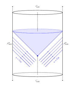
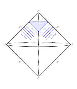
As we see it, the Bondi gauge is well-adapted for each type of asymptotics (see figure 2.1), while the Fefferman-Graham gauge is only defined in asymptotically (A)dS spacetimes.
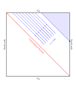
Refer to caption Refer to caption Refer to caption
AdS case (Λ<0)Λ0(\Lambda<0). Flat case (Λ=0)Λ0(\Lambda=0). dS case (Λ>0)Λ0(\Lambda>0).
Figure 2.1: Bondi gauge for any ΛΛ\Lambda.

2.2.3 Solution space

Definition [Solution space]

Given a gauge fixing (2.2.7) and boundary conditions, a solution of the theory is a field configuration ϕ~~italic-ϕ\tilde{\phi} satisfying G[ϕ~]=0𝐺delimited-[]~italic-ϕ0G[\tilde{\phi}]=0, the boundary conditions, and the Euler Lagrange-equations

δ𝐋δϕi|ϕ~=0,evaluated-at𝛿𝐋𝛿superscriptitalic-ϕ𝑖~italic-ϕ0\left.\frac{\delta\mathbf{L}}{\delta\phi^{i}}\right|_{\tilde{\phi}}=0, (2.2.25)

where the Euler-Lagrange derivative is defined in equation (A.2.1). The set of all solutions of the theory is called the solution space. It is parametrized as ϕ~=ϕ~(b)~italic-ϕ~italic-ϕ𝑏\tilde{\phi}=\tilde{\phi}(b), where the parameters b𝑏b are arbitrary functions of (n1)𝑛1(n-1) coordinates.

Examples

We now provide some examples of solution spaces of four-dimensional general relativity in different gauge fixings. These examples will be re-discussed in details in the remaining of the text (see e.g. subsections 6.2.1 and 6.2.2). We first consider the Fefferman-Graham gauge in asymptotically (A)dS4 spacetimes with preliminary boundary conditions (2.2.19). Solving the Einstein equations

Gμν+Λgμν=0,subscript𝐺𝜇𝜈Λsubscript𝑔𝜇𝜈0G_{\mu\nu}+\Lambda g_{\mu\nu}=0, (2.2.26)

we obtain the following analytic fall-offs:

γab=ρ2gab(0)+ρ1gab(1)+gab(2)+ρgab(3)+𝒪(ρ2),subscript𝛾𝑎𝑏superscript𝜌2superscriptsubscript𝑔𝑎𝑏0superscript𝜌1superscriptsubscript𝑔𝑎𝑏1superscriptsubscript𝑔𝑎𝑏2𝜌superscriptsubscript𝑔𝑎𝑏3𝒪superscript𝜌2\gamma_{ab}=\rho^{-2}g_{ab}^{(0)}+\rho^{-1}g_{ab}^{(1)}+g_{ab}^{(2)}+\rho g_{ab}^{(3)}+\mathcal{O}(\rho^{2}), (2.2.27)

where gab(i)subscriptsuperscript𝑔𝑖𝑎𝑏g^{(i)}_{ab} are functions of xasuperscript𝑥𝑎x^{a} [152, 153, 154, 155, 156]. The only free data in this expansion are gab(0)superscriptsubscript𝑔𝑎𝑏0g_{ab}^{(0)} and gab(3)superscriptsubscript𝑔𝑎𝑏3g_{ab}^{(3)}. All the other coefficients are determined in terms of these free data. Following the holographic dictionary, we call gab(0)superscriptsubscript𝑔𝑎𝑏0g_{ab}^{(0)} the boundary metric and we define

Tab=3|Λ|16πGgab(3)subscript𝑇𝑎𝑏3Λ16𝜋𝐺superscriptsubscript𝑔𝑎𝑏3T_{ab}=\frac{\sqrt{3|\Lambda|}}{16\pi G}g_{ab}^{(3)} (2.2.28)

as the stress energy tensor. From the Einstein equations, we have

gab(0)Tab=0,Da(0)Tab=0,formulae-sequencesuperscriptsubscript𝑔𝑎𝑏0superscript𝑇𝑎𝑏0superscriptsubscript𝐷𝑎0superscript𝑇𝑎𝑏0g_{ab}^{(0)}T^{ab}=0,\quad D_{a}^{(0)}T^{ab}=0, (2.2.29)

where Da(0)superscriptsubscript𝐷𝑎0D_{a}^{(0)} is the covariant derivative with respect to gab(0)superscriptsubscript𝑔𝑎𝑏0g_{ab}^{(0)}. In summary, the solution space of general relativity in the Fefferman-Graham gauge with the preliminary boundary condition (2.2.19) is parametrized by the set of functions

{gab(0),Tab}Λ0,subscriptsuperscriptsubscript𝑔𝑎𝑏0subscript𝑇𝑎𝑏Λ0\{g_{ab}^{(0)},T_{ab}\}_{\Lambda\neq 0}, (2.2.30)

where Tabsubscript𝑇𝑎𝑏T_{ab} satisfies (2.2.29) (111111 functions).

Now, for the restricted set of boundary conditions (2.2.21), that is, (AAdS1), the solution space reduces to

{gAB(0),Tab}Λ0,subscriptsuperscriptsubscript𝑔𝐴𝐵0subscript𝑇𝑎𝑏Λ0\{g_{AB}^{(0)},T_{ab}\}_{\Lambda\neq 0}, (2.2.31)

where gAB(0)superscriptsubscript𝑔𝐴𝐵0g_{AB}^{(0)} has a fixed determinant and Tabsubscript𝑇𝑎𝑏T_{ab} satisfies (2.2.29) (777 functions). Finally, for Dirichlet boundary conditions (2.2.23) (AAdS2), the solution space reduces to

{Tab}Λ0,subscriptsubscript𝑇𝑎𝑏Λ0\{T_{ab}\}_{\Lambda\neq 0}, (2.2.32)

where Tabsubscript𝑇𝑎𝑏T_{ab} satisfies (2.2.29) (5 functions).

Let us now consider the Bondi gauge in asymptotically (A)dS4 spacetimes with preliminary boundary condition (2.2.20). From the Fefferman-Graham theorem and the gauge matching between Bondi and Fefferman-Graham that is described in appendix D (see also [167, 166]), we know that the functions appearing in the metric admit an analytic expansion in powers of r𝑟r. In particular, we can write

gAB=r2qAB+rCAB+DAB+1rEAB+1r2FAB+𝒪(r3),subscript𝑔𝐴𝐵superscript𝑟2subscript𝑞𝐴𝐵𝑟subscript𝐶𝐴𝐵subscript𝐷𝐴𝐵1𝑟subscript𝐸𝐴𝐵1superscript𝑟2subscript𝐹𝐴𝐵𝒪superscript𝑟3g_{AB}=r^{2}q_{AB}+rC_{AB}+D_{AB}+\frac{1}{r}E_{AB}+\frac{1}{r^{2}}F_{AB}+\mathcal{O}(r^{-3}), (2.2.33)

where qABsubscript𝑞𝐴𝐵q_{AB}, CABsubscript𝐶𝐴𝐵C_{AB}, DABsubscript𝐷𝐴𝐵D_{AB}, EABsubscript𝐸𝐴𝐵E_{AB}, FABsubscript𝐹𝐴𝐵F_{AB}, \ldots are functions of (u,xA)𝑢superscript𝑥𝐴(u,x^{A}). The determinant condition defining the Bondi gauge and appearing in the third equation of (2.2.10) implies gABrgAB=4/rsuperscript𝑔𝐴𝐵subscript𝑟subscript𝑔𝐴𝐵4𝑟g^{AB}\partial_{r}g_{AB}=4/r, which imposes successively that det(gAB)=r4det(qAB)subscript𝑔𝐴𝐵superscript𝑟4subscript𝑞𝐴𝐵\det(g_{AB})=r^{4}\det(q_{AB}), qABCAB=0superscript𝑞𝐴𝐵subscript𝐶𝐴𝐵0q^{AB}C_{AB}=0 and

DAB=14qABCCDCCD+𝒟AB(u,xC),EAB=12qAB𝒟CDCCD+AB(u,xC),FAB=12qAB[CCDCD+12𝒟CD𝒟CD132(CCDCCD)2]+AB(u,xC),formulae-sequencesubscript𝐷𝐴𝐵14subscript𝑞𝐴𝐵superscript𝐶𝐶𝐷subscript𝐶𝐶𝐷subscript𝒟𝐴𝐵𝑢superscript𝑥𝐶formulae-sequencesubscript𝐸𝐴𝐵12subscript𝑞𝐴𝐵subscript𝒟𝐶𝐷superscript𝐶𝐶𝐷subscript𝐴𝐵𝑢superscript𝑥𝐶subscript𝐹𝐴𝐵12subscript𝑞𝐴𝐵delimited-[]superscript𝐶𝐶𝐷subscript𝐶𝐷12superscript𝒟𝐶𝐷subscript𝒟𝐶𝐷132superscriptsuperscript𝐶𝐶𝐷subscript𝐶𝐶𝐷2subscript𝐴𝐵𝑢superscript𝑥𝐶\begin{split}&D_{AB}=\frac{1}{4}q_{AB}C^{CD}C_{CD}+\mathcal{D}_{AB}(u,x^{C}),\\ &E_{AB}=\frac{1}{2}q_{AB}\mathcal{D}_{CD}C^{CD}+\mathcal{E}_{AB}(u,x^{C}),\\ &F_{AB}=\frac{1}{2}q_{AB}\Big{[}C^{CD}\mathcal{E}_{CD}+\frac{1}{2}\mathcal{D}^{CD}\mathcal{D}_{CD}-\frac{1}{32}(C^{CD}C_{CD})^{2}\Big{]}+\mathcal{F}_{AB}(u,x^{C}),\end{split} (2.2.34)

with qAB𝒟AB=qABAB=qABAB=0superscript𝑞𝐴𝐵subscript𝒟𝐴𝐵superscript𝑞𝐴𝐵subscript𝐴𝐵superscript𝑞𝐴𝐵subscript𝐴𝐵0q^{AB}\mathcal{D}_{AB}=q^{AB}\mathcal{E}_{AB}=q^{AB}\mathcal{F}_{AB}=0 (indices are lowered and raised with the metric qABsubscript𝑞𝐴𝐵q_{AB} and its inverse). We now sketch the results obtained by solving the Einstein equations

Gμν+Λgμν=0subscript𝐺𝜇𝜈Λsubscript𝑔𝜇𝜈0G_{\mu\nu}+\Lambda g_{\mu\nu}=0 (2.2.35)

for Λ0Λ0\Lambda\neq 0 (we follow [166, 167]; see also [168] for the Newman-Penrose version). The component (rr)𝑟𝑟(rr) gives the following radial constraints on the Bondi functions:

β(u,r,xA)𝛽𝑢𝑟superscript𝑥𝐴\displaystyle\beta(u,r,x^{A}) =β0(u,xA)+1r2[132CABCAB]+1r3[112CAB𝒟AB]absentsubscript𝛽0𝑢superscript𝑥𝐴1superscript𝑟2delimited-[]132superscript𝐶𝐴𝐵subscript𝐶𝐴𝐵1superscript𝑟3delimited-[]112superscript𝐶𝐴𝐵subscript𝒟𝐴𝐵\displaystyle=\beta_{0}(u,x^{A})+\frac{1}{r^{2}}\Big{[}-\frac{1}{32}C^{AB}C_{AB}\Big{]}+\frac{1}{r^{3}}\Big{[}-\frac{1}{12}C^{AB}\mathcal{D}_{AB}\Big{]} (2.2.36)
+1r4[332CABAB116𝒟AB𝒟AB+1128(CABCAB)2]+𝒪(r5).1superscript𝑟4delimited-[]332superscript𝐶𝐴𝐵subscript𝐴𝐵116superscript𝒟𝐴𝐵subscript𝒟𝐴𝐵1128superscriptsuperscript𝐶𝐴𝐵subscript𝐶𝐴𝐵2𝒪superscript𝑟5\displaystyle\qquad+\frac{1}{r^{4}}\Big{[}-\frac{3}{32}C^{AB}\mathcal{E}_{AB}-\frac{1}{16}\mathcal{D}^{AB}\mathcal{D}_{AB}+\frac{1}{128}(C^{AB}C_{AB})^{2}\Big{]}+\mathcal{O}(r^{-5}).

where β0(u,xA)subscript𝛽0𝑢superscript𝑥𝐴\beta_{0}(u,x^{A}) is an arbitrary function. The component (rA)𝑟𝐴(rA) yields

UA=U0A(u,xB)+UA(1)(u,xB)1r+UA(2)(u,xB)1r2+UA(3)(u,xB)1r3+UA(L3)(u,xB)lnrr3+o(r3)superscript𝑈𝐴subscriptsuperscript𝑈𝐴0𝑢superscript𝑥𝐵1superscript𝑈𝐴𝑢superscript𝑥𝐵1𝑟2superscript𝑈𝐴𝑢superscript𝑥𝐵1superscript𝑟23superscript𝑈𝐴𝑢superscript𝑥𝐵1superscript𝑟3L3superscript𝑈𝐴𝑢superscript𝑥𝐵𝑟superscript𝑟3𝑜superscript𝑟3\begin{split}U^{A}=\,\,&U^{A}_{0}(u,x^{B})+\overset{(1)}{U^{A}}(u,x^{B})\frac{1}{r}+\overset{(2)}{U^{A}}(u,x^{B})\frac{1}{r^{2}}\\ &+\overset{(3)}{U^{A}}(u,x^{B})\frac{1}{r^{3}}+\overset{(\text{L}3)}{U^{A}}(u,x^{B})\frac{\ln r}{r^{3}}+o(r^{-3})\end{split} (2.2.37)

with

UA(1)(u,xB)1superscript𝑈𝐴𝑢superscript𝑥𝐵\displaystyle\overset{(1)}{U^{A}}(u,x^{B}) =\displaystyle= 2e2β0Aβ0,2superscript𝑒2subscript𝛽0superscript𝐴subscript𝛽0\displaystyle 2e^{2\beta_{0}}\partial^{A}\beta_{0},
UA(2)(u,xB)2superscript𝑈𝐴𝑢superscript𝑥𝐵\displaystyle\overset{(2)}{U^{A}}(u,x^{B}) =\displaystyle= e2β0[CABBβ0+12DBCAB],superscript𝑒2subscript𝛽0delimited-[]superscript𝐶𝐴𝐵subscript𝐵subscript𝛽012subscript𝐷𝐵superscript𝐶𝐴𝐵\displaystyle-e^{2\beta_{0}}\Big{[}C^{AB}\partial_{B}\beta_{0}+\frac{1}{2}D_{B}C^{AB}\Big{]},
UA(3)(u,xB)3superscript𝑈𝐴𝑢superscript𝑥𝐵\displaystyle\overset{(3)}{U^{A}}(u,x^{B}) =\displaystyle= 23e2β0[NA12CABDCCBC+(Bβ013DB)𝒟AB316CCDCCDAβ0],23superscript𝑒2subscript𝛽0delimited-[]superscript𝑁𝐴12superscript𝐶𝐴𝐵superscript𝐷𝐶subscript𝐶𝐵𝐶subscript𝐵subscript𝛽013subscript𝐷𝐵superscript𝒟𝐴𝐵316subscript𝐶𝐶𝐷superscript𝐶𝐶𝐷superscript𝐴subscript𝛽0\displaystyle-\frac{2}{3}e^{2\beta_{0}}\Big{[}N^{A}-\frac{1}{2}C^{AB}D^{C}C_{BC}+(\partial_{B}\beta_{0}-\frac{1}{3}D_{B})\mathcal{D}^{AB}-\frac{3}{16}C_{CD}C^{CD}\partial^{A}\beta_{0}\Big{]},
UA(L3)(u,xB)L3superscript𝑈𝐴𝑢superscript𝑥𝐵\displaystyle\overset{(\text{L}3)}{U^{A}}(u,x^{B}) =\displaystyle= 23e2β0DB𝒟AB.23superscript𝑒2subscript𝛽0subscript𝐷𝐵superscript𝒟𝐴𝐵\displaystyle-\frac{2}{3}e^{2\beta_{0}}D_{B}\mathcal{D}^{AB}. (2.2.38)

In these expressions, U0A(u,xB)subscriptsuperscript𝑈𝐴0𝑢superscript𝑥𝐵U^{A}_{0}(u,x^{B}) and NA(u,xB)superscript𝑁𝐴𝑢superscript𝑥𝐵N^{A}(u,x^{B}) are arbitrary functions. We call NAsuperscript𝑁𝐴N^{A} the angular momentum aspect. Notice that, at this stage, logarithmic terms are appearing in the expansion (2.2.37). However, we will see below that these terms vanish for Λ0Λ0\Lambda\neq 0. The component (ru)𝑟𝑢(ru) leads to

Vr=𝑉𝑟absent\displaystyle\frac{V}{r}= Λ3e2β0r2r(l+DAU0A)Λ3superscript𝑒2subscript𝛽0superscript𝑟2𝑟𝑙subscript𝐷𝐴subscriptsuperscript𝑈𝐴0\displaystyle\frac{\Lambda}{3}e^{2\beta_{0}}r^{2}-r(l+D_{A}U^{A}_{0}) (2.2.39)
e2β0[12(R[q]+Λ8CABCAB)+2DAAβ0+4Aβ0Aβ0]2Mr+o(r1),superscript𝑒2subscript𝛽0delimited-[]12𝑅delimited-[]𝑞Λ8subscript𝐶𝐴𝐵superscript𝐶𝐴𝐵2subscript𝐷𝐴superscript𝐴subscript𝛽04subscript𝐴subscript𝛽0superscript𝐴subscript𝛽02𝑀𝑟𝑜superscript𝑟1\displaystyle-e^{2\beta_{0}}\Big{[}\frac{1}{2}\Big{(}R[q]+\frac{\Lambda}{8}C_{AB}C^{AB}\Big{)}+2D_{A}\partial^{A}\beta_{0}+4\partial_{A}\beta_{0}\partial^{A}\beta_{0}\Big{]}-\frac{2M}{r}+o(r^{-1}),

where l=ulnq𝑙subscript𝑢𝑞l=\partial_{u}\ln\sqrt{q}, R[q]𝑅delimited-[]𝑞R[q] is the scalar curvature associated with the metric qABsubscript𝑞𝐴𝐵q_{AB} and M(u,xA)𝑀𝑢superscript𝑥𝐴M(u,x^{A}) is an arbitrary function called the Bondi mass aspect. Afterwards, we solve the components (AB)𝐴𝐵(AB) of the Einstein equations order by order, thereby providing us with the constraints imposed on each order of gABsubscript𝑔𝐴𝐵g_{AB}. The leading order 𝒪(r1)𝒪superscript𝑟1\mathcal{O}(r^{-1}) of that equation yields to

Λ3CAB=e2β0[(ul)qAB+2D(AUB)0DCUC0qAB].\frac{\Lambda}{3}C_{AB}=e^{-2\beta_{0}}\Big{[}(\partial_{u}-l)q_{AB}+2D_{(A}U^{0}_{B)}-D^{C}U^{0}_{C}q_{AB}\Big{]}. (2.2.40)

Going to 𝒪(r2)𝒪superscript𝑟2\mathcal{O}(r^{-2}), we get

Λ3𝒟AB=0,Λ3subscript𝒟𝐴𝐵0\frac{\Lambda}{3}\mathcal{D}_{AB}=0, (2.2.41)

which removes the logarithmic term in (2.2.37) for Λ0Λ0\Lambda\neq 0 (but not for Λ=0Λ0\Lambda=0). The condition at the next order 𝒪(r3)𝒪superscript𝑟3\mathcal{O}(r^{-3})

u𝒟AB+U0CDC𝒟AB+2𝒟C(ADB)U0C=0\partial_{u}\mathcal{D}_{AB}+U_{0}^{C}D_{C}\mathcal{D}_{AB}+2\mathcal{D}_{C(A}D_{B)}U_{0}^{C}=0 (2.2.42)

is trivial for Λ0Λ0\Lambda\neq 0. Using an iterative argument as in [167], we now make the following observation. If we decompose gAB=r2n0gAB(n)rnsubscript𝑔𝐴𝐵superscript𝑟2subscript𝑛0superscriptsubscript𝑔𝐴𝐵𝑛superscript𝑟𝑛g_{AB}=r^{2}\sum_{n\geq 0}g_{AB}^{(n)}r^{-n}, we see that the iterative solution of the components (AB)𝐴𝐵(AB) of the Einstein equations organizes itself as ΛgAB(n)=ugAB(n1)+()Λsuperscriptsubscript𝑔𝐴𝐵𝑛subscript𝑢superscriptsubscript𝑔𝐴𝐵𝑛1\Lambda g_{AB}^{(n)}=\partial_{u}g_{AB}^{(n-1)}+(...) at order 𝒪(rn)𝒪superscript𝑟𝑛\mathcal{O}(r^{-n}), n0𝑛subscript0n\in\mathbb{N}_{0}. Accordingly, the form of ABsubscript𝐴𝐵\mathcal{E}_{AB} should have been fixed by the equation found at 𝒪(r3)𝒪superscript𝑟3\mathcal{O}(r^{-3}); however, this is not the case, since both contributions of ABsubscript𝐴𝐵\mathcal{E}_{AB} cancel between GABsubscript𝐺𝐴𝐵G_{AB} and ΛgABΛsubscript𝑔𝐴𝐵\Lambda g_{AB}. Moreover, the equation ΛgAB(4)=ugAB(3)+()Λsuperscriptsubscript𝑔𝐴𝐵4subscript𝑢superscriptsubscript𝑔𝐴𝐵3\Lambda g_{AB}^{(4)}=\partial_{u}g_{AB}^{(3)}+(...) at the next order turns out to be a constraint for gAB(4)ABsimilar-tosuperscriptsubscript𝑔𝐴𝐵4subscript𝐴𝐵g_{AB}^{(4)}\sim\mathcal{F}_{AB}, determined with other subleading data such as CABsubscript𝐶𝐴𝐵C_{AB} or ugAB(3)uABsimilar-tosubscript𝑢superscriptsubscript𝑔𝐴𝐵3subscript𝑢subscript𝐴𝐵\partial_{u}g_{AB}^{(3)}\sim\partial_{u}\mathcal{E}_{AB}. It shows that ABsubscript𝐴𝐵\mathcal{E}_{AB} is a set of two free data on the boundary, built up from two arbitrary functions of (u,xA)𝑢superscript𝑥𝐴(u,x^{A}). Morover, it indicates that no more data exist to be uncovered for Λ0Λ0\Lambda\neq 0. Finally, the components (uu)𝑢𝑢(uu) and (uA)𝑢𝐴(uA) of the Einstein equations give some evolution constraints with respect to the u𝑢u coordinate for the Bondi mass aspect M𝑀M and the angular momentum aspect NAsuperscript𝑁𝐴N^{A}. We will not describe these equations explicitly here (see [167, 166] or subsection 6.2.2).

In summary, the solution space for general relativity in the Bondi gauge with the preliminary boundary condition (2.2.33) and Λ0Λ0\Lambda\neq 0 is parametrized by the set of functions

{β0,U0A,qAB,AB,M,NA}Λ0subscriptsubscript𝛽0subscriptsuperscript𝑈𝐴0subscript𝑞𝐴𝐵subscript𝐴𝐵𝑀superscript𝑁𝐴Λ0\{\beta_{0},U^{A}_{0},q_{AB},\mathcal{E}_{AB},M,N^{A}\}_{\Lambda\neq 0} (2.2.43)

(111111 functions), where M𝑀M and NAsuperscript𝑁𝐴N^{A} have constrained evolutions with respect to the u𝑢u coordinate. Therefore, the characteristic initial value problem is well-defined when the following data are given: β0(u,xC)subscript𝛽0𝑢superscript𝑥𝐶\beta_{0}(u,x^{C}), U0A(u,xC)subscriptsuperscript𝑈𝐴0𝑢superscript𝑥𝐶U^{A}_{0}(u,x^{C}), AB(u,xC)subscript𝐴𝐵𝑢superscript𝑥𝐶\mathcal{E}_{AB}(u,x^{C}), qAB(u,xC)subscript𝑞𝐴𝐵𝑢superscript𝑥𝐶q_{AB}(u,x^{C}), M(u0,xC)𝑀subscript𝑢0superscript𝑥𝐶M(u_{0},x^{C}) and NA(u0,xC)superscript𝑁𝐴subscript𝑢0superscript𝑥𝐶N^{A}(u_{0},x^{C}), where u0subscript𝑢0u_{0} is a fixed value of u𝑢u.

Notice that for the boundary conditions (2.2.22) (AAdS1), the solution space reduces to

{qAB,AB,M,NA}Λ0,subscriptsubscript𝑞𝐴𝐵subscript𝐴𝐵𝑀superscript𝑁𝐴Λ0\{q_{AB},\mathcal{E}_{AB},M,N^{A}\}_{\Lambda\neq 0}, (2.2.44)

where M𝑀M and NAsuperscript𝑁𝐴N^{A} have constrained evolutions with respect to the u𝑢u coordinate, and qABsubscript𝑞𝐴𝐵q_{AB} has a fixed determinant [166] (777 functions). Finally, for the Dirichlet boundary conditions (2.2.24) (AAdS2), the solution space finally reduces to

{AB,M,NA}Λ0,subscriptsubscript𝐴𝐵𝑀superscript𝑁𝐴Λ0\{\mathcal{E}_{AB},M,N^{A}\}_{\Lambda\neq 0}, (2.2.45)

where M𝑀M and NAsuperscript𝑁𝐴N^{A} have constrained evolutions with respect to the u𝑢u coordinate (5 functions).

Let us finally discuss the Bondi gauge in asymptotically flat spacetimes [1, 2, 3, 6, 169, 8, 166]. We first consider the preliminary boundary conditions (2.2.15). From the previous analysis of solution space with Λ0Λ0\Lambda\neq 0, we can readily obtain the solution space with Λ=0Λ0\Lambda=0, that is, the solution of

Gμν=0,subscript𝐺𝜇𝜈0G_{\mu\nu}=0, (2.2.46)

by taking the flat limit Λ0Λ0\Lambda\to 0. The radial constraints (2.2.36), (2.2.38) and (2.2.39) are still valid by setting to zero β0subscript𝛽0\beta_{0}, U0Asubscriptsuperscript𝑈𝐴0U^{A}_{0} (see equation (2.2.15)) and all the terms proportional to ΛΛ\Lambda. Furthermore, by the same procedure, the constraint equation (2.2.40) becomes

(ul)qAB=0.subscript𝑢𝑙subscript𝑞𝐴𝐵0(\partial_{u}-l)q_{AB}=0. (2.2.47)

Therefore, the asymptotic shear CABsubscript𝐶𝐴𝐵C_{AB} becomes unconstrained, and the metric qABsubscript𝑞𝐴𝐵q_{AB} gets a time evolution constraint. Similarly, the equation (2.2.41) becomes trivial and 𝒟ABsubscript𝒟𝐴𝐵\mathcal{D}_{AB} is not constrained at this order. In particular, this allows for the existence of logarithmic terms in the Bondi expansion (see equation (2.2.37)). One has to impose the additional condition DA𝒟AB=0superscript𝐷𝐴subscript𝒟𝐴𝐵0D^{A}\mathcal{D}_{AB}=0 to make these logarithmic terms disappear. Finally, one can see that for Λ=0Λ0\Lambda=0, the subleading orders of the components (AB)𝐴𝐵(AB) of the Einstein equations impose time evolution constraints on 𝒟ABsubscript𝒟𝐴𝐵\mathcal{D}_{AB}, ABsubscript𝐴𝐵\mathcal{E}_{AB}, \ldots , but this infinite tower of functions is otherwise unconstrained and they become free parameters of the solution space. Finally, as for the case Λ0Λ0\Lambda\neq 0, the components (uu)𝑢𝑢(uu) and (uA)𝑢𝐴(uA) of the Einstein equations yield time evolution constraints for the Bondi mass aspect M𝑀M and the angular momentum aspect NAsuperscript𝑁𝐴N^{A}.

In summary, the solution space for general relativity in the Bondi gauge with the preliminary boundary condition (2.2.15) is parametrized by the set of functions

{qAB,CAB,M,NA,𝒟AB,AB,AB,}Λ=0,subscriptsubscript𝑞𝐴𝐵subscript𝐶𝐴𝐵𝑀superscript𝑁𝐴subscript𝒟𝐴𝐵subscript𝐴𝐵subscript𝐴𝐵Λ0\{q_{AB},C_{AB},M,N^{A},\mathcal{D}_{AB},\mathcal{E}_{AB},\mathcal{F}_{AB},\ldots\}_{\Lambda=0}, (2.2.48)

where qABsubscript𝑞𝐴𝐵q_{AB}, M𝑀M, NAsuperscript𝑁𝐴N^{A}, 𝒟ABsubscript𝒟𝐴𝐵\mathcal{D}_{AB}, ABsubscript𝐴𝐵\mathcal{E}_{AB}, ABsubscript𝐴𝐵\mathcal{F}_{AB}, \ldots have constrained time evolutions (infinite tower of independent functions). Therefore, the characteristic initial value problem is well-defined when the following data are given: CAB(u,cC)subscript𝐶𝐴𝐵𝑢superscript𝑐𝐶C_{AB}(u,c^{C}), qAB(u0,xC)subscript𝑞𝐴𝐵subscript𝑢0superscript𝑥𝐶q_{AB}(u_{0},x^{C}), M(u0,xC)𝑀subscript𝑢0superscript𝑥𝐶M(u_{0},x^{C}), NA(u0,xC)superscript𝑁𝐴subscript𝑢0superscript𝑥𝐶N^{A}(u_{0},x^{C}), 𝒟AB(u0,xC)subscript𝒟𝐴𝐵subscript𝑢0superscript𝑥𝐶\mathcal{D}_{AB}(u_{0},x^{C}), AB(u0,xC)subscript𝐴𝐵subscript𝑢0superscript𝑥𝐶\mathcal{E}_{AB}(u_{0},x^{C}), AB(u0,xC)subscript𝐴𝐵subscript𝑢0superscript𝑥𝐶\mathcal{F}_{AB}(u_{0},x^{C}), \ldots where u0subscript𝑢0u_{0} is a fixed value of u𝑢u. Notice a subtle point here: by taking the flat limit of the solution space with Λ0Λ0\Lambda\neq 0, we assumed that gABsubscript𝑔𝐴𝐵g_{AB} is analytic in r𝑟r and can be expanded as (2.2.33) (this condition was not restrictive for Λ0Λ0\Lambda\neq 0). This condition is slightly more restrictive than (2.2.15) where analyticity is assumed only up to order r1superscript𝑟1r^{-1}. Therefore, by this flat limit procedure, we only obtain a subsector of the most general solution space. Writing gAB(u,r,xC)=r2qAB(u,xC)+rCAB(u,xC)+DAB(u,xC)+E~AB(u,r,xC)subscript𝑔𝐴𝐵𝑢𝑟superscript𝑥𝐶superscript𝑟2subscript𝑞𝐴𝐵𝑢superscript𝑥𝐶𝑟subscript𝐶𝐴𝐵𝑢superscript𝑥𝐶subscript𝐷𝐴𝐵𝑢superscript𝑥𝐶subscript~𝐸𝐴𝐵𝑢𝑟superscript𝑥𝐶g_{AB}(u,r,x^{C})=r^{2}q_{AB}(u,x^{C})+rC_{AB}(u,x^{C})+D_{AB}(u,x^{C})+\tilde{E}_{AB}(u,r,x^{C}), where E~ABsubscript~𝐸𝐴𝐵\tilde{E}_{AB} is a function of all the coordinates of order 𝒪(r1)𝒪superscript𝑟1\mathcal{O}(r^{-1}) in r𝑟r, the most general solution space can be written as

{qAB,CAB,M,NA,𝒟AB,~AB}Λ=0,subscriptsubscript𝑞𝐴𝐵subscript𝐶𝐴𝐵𝑀superscript𝑁𝐴subscript𝒟𝐴𝐵subscript~𝐴𝐵Λ0\{q_{AB},C_{AB},M,N^{A},\mathcal{D}_{AB},\tilde{\mathcal{E}}_{AB}\}_{\Lambda=0}, (2.2.49)

where ~ABsubscript~𝐴𝐵\tilde{\mathcal{E}}_{AB} is the trace-free part of E~ABsubscript~𝐸𝐴𝐵\tilde{{E}}_{AB}, and qABsubscript𝑞𝐴𝐵q_{AB}, M𝑀M, NAsuperscript𝑁𝐴N^{A}, 𝒟ABsubscript𝒟𝐴𝐵\mathcal{D}_{AB}, ~ABsubscript~𝐴𝐵\tilde{\mathcal{E}}_{AB} obey time evolution constraints. Now, the characteristic initial value problem is well-defined when the following data are given: CAB(u,cC)subscript𝐶𝐴𝐵𝑢superscript𝑐𝐶C_{AB}(u,c^{C}), qAB(u0,xC)subscript𝑞𝐴𝐵subscript𝑢0superscript𝑥𝐶q_{AB}(u_{0},x^{C}), M(u0,xC)𝑀subscript𝑢0superscript𝑥𝐶M(u_{0},x^{C}), NA(u0,xC)superscript𝑁𝐴subscript𝑢0superscript𝑥𝐶N^{A}(u_{0},x^{C}), 𝒟AB(u0,xC)subscript𝒟𝐴𝐵subscript𝑢0superscript𝑥𝐶\mathcal{D}_{AB}(u_{0},x^{C}) and ~AB(u0,r,xC)subscript~𝐴𝐵subscript𝑢0𝑟superscript𝑥𝐶\tilde{\mathcal{E}}_{AB}(u_{0},r,x^{C}).

We complete this set of examples by mentioning the restricted solution spaces in the different definitions of asymptotic flatness introduced above. For boundary conditions (AF1) (equations (2.2.15) with (2.2.16)), we obtain

{qAB,CAB,M,NA,𝒟AB,~AB}Λ=0,subscriptsubscript𝑞𝐴𝐵subscript𝐶𝐴𝐵𝑀superscript𝑁𝐴subscript𝒟𝐴𝐵subscript~𝐴𝐵Λ0\{q_{AB},C_{AB},M,N^{A},\mathcal{D}_{AB},\tilde{\mathcal{E}}_{AB}\}_{\Lambda=0}, (2.2.50)

where qABsubscript𝑞𝐴𝐵q_{AB}, M𝑀M, NAsuperscript𝑁𝐴N^{A}, 𝒟ABsubscript𝒟𝐴𝐵\mathcal{D}_{AB} and ~ABsubscript~𝐴𝐵\tilde{\mathcal{E}}_{AB} obey time evolution constraints, and q𝑞\sqrt{q} is fixed. In particular, if we choose a branch where q𝑞\sqrt{q} is time-independent, from (2.2.47), we immediately see that uqAB=0subscript𝑢subscript𝑞𝐴𝐵0\partial_{u}q_{AB}=0. For boundary conditions (AF2) (equations (2.2.15) with (2.2.17)), the solution space reduces to

{φ,CAB,M,NA,𝒟AB,~AB}Λ=0,subscript𝜑subscript𝐶𝐴𝐵𝑀superscript𝑁𝐴subscript𝒟𝐴𝐵subscript~𝐴𝐵Λ0\{\varphi,C_{AB},M,N^{A},\mathcal{D}_{AB},\tilde{\mathcal{E}}_{AB}\}_{\Lambda=0}, (2.2.51)

where M𝑀M, NAsuperscript𝑁𝐴N^{A}, 𝒟ABsubscript𝒟𝐴𝐵\mathcal{D}_{AB} and ~ABsubscript~𝐴𝐵\tilde{\mathcal{E}}_{AB} obey time evolution equations. Notice that the metric qABsubscript𝑞𝐴𝐵q_{AB} of the form (2.2.17) automatically satisfies (2.2.47). This agrees with results of [6]. Finally, taking the boundary conditions (AF3) (equations (2.2.15) with (2.2.18)) yields the solution space

{CAB,M,NA,𝒟AB,~AB}Λ=0,subscriptsubscript𝐶𝐴𝐵𝑀superscript𝑁𝐴subscript𝒟𝐴𝐵subscript~𝐴𝐵Λ0\{C_{AB},M,N^{A},\mathcal{D}_{AB},\tilde{\mathcal{E}}_{AB}\}_{\Lambda=0}, (2.2.52)

where M𝑀M, NAsuperscript𝑁𝐴N^{A}, 𝒟ABsubscript𝒟𝐴𝐵\mathcal{D}_{AB} and ~ABsubscript~𝐴𝐵\tilde{\mathcal{E}}_{AB} obey time evolution equations. This agrees with the historical results of [1, 2, 3].

2.2.4 Asymptotic symmetry algebra

Definition [Asymptotic symmetry]

Given boundary conditions imposed in a chosen gauge, the asymptotic symmetries are defined as the residual gauge transformations preserving the boundary conditions666This is the weak definition of asymptotic symmetry, in the sense of (2.1.2).. In other words, the asymptotic symmetries considered on-shell are the gauge transformations R[f]𝑅delimited-[]𝑓R[f] tangent to the solution space. In practice, the requirement to preserve the boundary conditions gives some constraints on the functions parametrizing the residual gauge transformations. In gravity, the generators of asymptotic symmetries are often called asymptotic Killing vectors.

Definition [Asymptotic symmetry algebra]

Once the asymptotic symmetries are known, we have

[R[f1],R[f2]]=δf1R[f2]δf2R[f1]R[[f1,f2]A],𝑅delimited-[]subscript𝑓1𝑅delimited-[]subscript𝑓2subscript𝛿subscript𝑓1𝑅delimited-[]subscript𝑓2subscript𝛿subscript𝑓2𝑅delimited-[]subscript𝑓1𝑅delimited-[]subscriptsubscript𝑓1subscript𝑓2𝐴\begin{split}[R[f_{1}],R[f_{2}]]&=\delta_{f_{1}}R[f_{2}]-\delta_{f_{2}}R[f_{1}]\\ &\approx R[[f_{1},f_{2}]_{A}],\end{split} (2.2.53)

where \approx means that this equality holds on-shell, i.e. on the solution space. In this expression, the bracket [f1,f2]Asubscriptsubscript𝑓1subscript𝑓2𝐴[f_{1},f_{2}]_{A} of gauge symmetry generators is given by

[f1,f2]A=C(f1,f2)δf1f2+δf2f1,subscriptsubscript𝑓1subscript𝑓2𝐴𝐶subscript𝑓1subscript𝑓2subscript𝛿subscript𝑓1subscript𝑓2subscript𝛿subscript𝑓2subscript𝑓1[f_{1},f_{2}]_{A}=C(f_{1},f_{2})-\delta_{f_{1}}f_{2}+\delta_{f_{2}}f_{1}, (2.2.54)

where C(f1,f2)𝐶subscript𝑓1subscript𝑓2C(f_{1},f_{2}) is a skew-symmetric bi-differential operator [170, 171]

C(f1,f2)=k,l0C[αβ](μ1μk)(ν1νl)μ1μkf1αν1νlf2β.𝐶subscript𝑓1subscript𝑓2subscript𝑘𝑙0subscriptsuperscript𝐶subscript𝜇1subscript𝜇𝑘subscript𝜈1subscript𝜈𝑙delimited-[]𝛼𝛽subscriptsubscript𝜇1subscriptsubscript𝜇𝑘subscriptsuperscript𝑓𝛼1subscriptsubscript𝜈1subscriptsubscript𝜈𝑙superscriptsubscript𝑓2𝛽C(f_{1},f_{2})=\sum_{k,l\geq 0}C^{(\mu_{1}\cdots\mu_{k})(\nu_{1}\cdots\nu_{l})}_{[\alpha\beta]}\partial_{\mu_{1}}\ldots\partial_{\mu_{k}}f^{\alpha}_{1}\partial_{\nu_{1}}\ldots\partial_{\nu_{l}}f_{2}^{\beta}. (2.2.55)

The presence of the terms δf1f2+δf2f1subscript𝛿subscript𝑓1subscript𝑓2subscript𝛿subscript𝑓2subscript𝑓1-\delta_{f_{1}}f_{2}+\delta_{f_{2}}f_{1} in (2.2.53) is due to the possible field-dependence of the asymptotic symmetry generators. We can verify that (2.2.54) satisfies the Jacobi identity, i.e. the asymptotic symmetry generators form a (solution space-dependent) Lie algebra for this bracket. It is called the asymptotic symmetry algebra. The statement (2.2.53) means that the infinitesimal action of the gauge symmetries on the fields forms a representation of the Lie algebra of asymptotic symmetry generators: [δf1,δf2]ϕ=δ[f1,f2]Aϕsubscript𝛿subscript𝑓1subscript𝛿subscript𝑓2italic-ϕsubscript𝛿subscriptsubscript𝑓1subscript𝑓2𝐴italic-ϕ[\delta_{f_{1}},\delta_{f_{2}}]\phi=\delta_{[f_{1},f_{2}]_{A}}\phi. Let us mention that a Lie algebroid structure is showing up at this stage [172, 170, 146]. The base manifold is given by the solution space, the field-dependent Lie algebra is the Lie algebra of asymptotic symmetry generators introduced above and the anchor is the map fR[f]𝑓𝑅delimited-[]𝑓f\to R[f].

Examples

The examples that we present here will be re-discussed in much details in the remaining of the text. Let us start by considering asymptotically AdS4 spacetimes in the Fefferman-Graham and Bondi gauge. The preliminary boundary condition (2.2.19) does not impose any constraint on the generators of the residual gauge diffeomorphisms of the Fefferman-Graham gauge given in (2.2.13). Similarly, the generators of the residual gauge diffeomorphisms in Bondi gauge given in (2.2.14) do not get further constraints with (2.2.20).

Now, let us consider the boundary conditions (AAdS1) (equation (2.2.19) together with (2.2.21)) in the Fefferman-Graham gauge. The asymptotic symmetries are generated by the vectors fields ξμsuperscript𝜉𝜇\xi^{\mu} given in (2.2.13) preserving the boundary conditions, namely, satisfying ξgtt(0)=0subscript𝜉superscriptsubscript𝑔𝑡𝑡00\mathcal{L}_{\xi}g_{tt}^{(0)}=0, ξgtA(0)=0subscript𝜉superscriptsubscript𝑔𝑡𝐴00\mathcal{L}_{\xi}g_{tA}^{(0)}=0 and g(0)abξgab(0)=0subscriptsuperscript𝑔𝑎𝑏0subscript𝜉superscriptsubscript𝑔𝑎𝑏00g^{ab}_{(0)}\mathcal{L}_{\xi}g_{ab}^{(0)}=0. This leads to the following constraints on the parameters:

(u12l)ξ0t=12DA(0)ξ0A,uYA=Λ3g(0)ABBξ0t,σ=12(DA(0)ξ0A+ξ0tl),formulae-sequencesubscript𝑢12𝑙superscriptsubscript𝜉0𝑡12superscriptsubscript𝐷𝐴0subscriptsuperscript𝜉𝐴0formulae-sequencesubscript𝑢superscript𝑌𝐴Λ3subscriptsuperscript𝑔𝐴𝐵0subscript𝐵superscriptsubscript𝜉0𝑡𝜎12superscriptsubscript𝐷𝐴0subscriptsuperscript𝜉𝐴0subscriptsuperscript𝜉𝑡0𝑙\left(\partial_{u}-\frac{1}{2}l\right)\xi_{0}^{t}=\frac{1}{2}D_{A}^{(0)}\xi^{A}_{0},\quad\partial_{u}Y^{A}=-\frac{\Lambda}{3}g^{AB}_{(0)}\partial_{B}\xi_{0}^{t},\quad\sigma=\frac{1}{2}(D_{A}^{(0)}\xi^{A}_{0}+\xi^{t}_{0}l), (2.2.56)

where l=ulnq¯𝑙subscript𝑢¯𝑞l=\partial_{u}\ln\sqrt{\bar{q}}. In this case, the Lie bracket (2.2.54) is given by

[ξ1,ξ2]A=ξ1ξ2δξ1ξ2+δξ2ξ1subscriptsubscript𝜉1subscript𝜉2𝐴subscriptsubscript𝜉1subscript𝜉2subscript𝛿subscript𝜉1subscript𝜉2subscript𝛿subscript𝜉2subscript𝜉1[\xi_{1},\xi_{2}]_{A}=\mathcal{L}_{\xi_{1}}\xi_{2}-\delta_{\xi_{1}}\xi_{2}+\delta_{\xi_{2}}\xi_{1} (2.2.57)

and is referred as the modified Lie bracket [6]. Therefore, the asymptotic symmetry algebra can be worked out and is given explicitly by [ξ(ξ0,1t,ξ0,1A),ξ(ξ0,2t,ξ0,2A)]A=ξ(ξ^0t,ξ^0A)subscript𝜉superscriptsubscript𝜉01𝑡subscriptsuperscript𝜉𝐴01𝜉superscriptsubscript𝜉02𝑡subscriptsuperscript𝜉𝐴02𝐴𝜉superscriptsubscript^𝜉0𝑡superscriptsubscript^𝜉0𝐴[\xi(\xi_{0,1}^{t},\xi^{A}_{0,1}),\xi(\xi_{0,2}^{t},\xi^{A}_{0,2})]_{A}=\xi({\hat{\xi}}_{0}^{t},{\hat{\xi}}_{0}^{A}), where777The terms δξ(ξ0,1t,ξ0,1A)ξ0,2tsubscript𝛿𝜉superscriptsubscript𝜉01𝑡subscriptsuperscript𝜉𝐴01superscriptsubscript𝜉02𝑡\delta_{\xi(\xi_{0,1}^{t},\xi^{A}_{0,1})}\xi_{0,2}^{t} and δξ(ξ0,1t,ξ0,1A)ξ0,2Asubscript𝛿𝜉superscriptsubscript𝜉01𝑡subscriptsuperscript𝜉𝐴01superscriptsubscript𝜉02𝐴\delta_{\xi(\xi_{0,1}^{t},\xi^{A}_{0,1})}\xi_{0,2}^{A} in (2.2.58) take into account the possible field-dependence of the parameters (ξ0,2t,ξ0,2A)superscriptsubscript𝜉02𝑡subscriptsuperscript𝜉𝐴02(\xi_{0,2}^{t},\xi^{A}_{0,2}).

ξ^0t=ξ0,1AAξ0,2t+12ξ0,1tDA(0)ξ0,2Aδξ(ξ0,1t,ξ0,1A)ξ0,2t(12),ξ^0A=ξ0,1BBξ0,2AΛ3ξ0,1tg(0)ABBξ0,2tδξ(ξ0,1t,ξ0,1A)ξ0,2A(12).\begin{split}{\hat{\xi}}_{0}^{t}&=\xi^{A}_{0,1}\partial_{A}\xi_{0,2}^{t}+\frac{1}{2}\xi_{0,1}^{t}D_{A}^{(0)}\xi^{A}_{0,2}-\delta_{\xi(\xi_{0,1}^{t},\xi^{A}_{0,1})}\xi_{0,2}^{t}-(1\leftrightarrow 2),\\ {\hat{\xi}}_{0}^{A}&={\xi}_{0,1}^{B}\partial_{B}\xi^{A}_{0,2}-\frac{\Lambda}{3}\xi_{0,1}^{t}g^{AB}_{(0)}\partial_{B}\xi_{0,2}^{t}-\delta_{\xi(\xi_{0,1}^{t},\xi^{A}_{0,1})}\xi_{0,2}^{A}-(1\leftrightarrow 2).\\ \end{split} (2.2.58)

In the Bondi gauge with corresponding boundary conditions (2.2.22), the constraints on the parameters are given by

(u12l)f=12DAYA,uYA=Λ3qABBf,ω=0formulae-sequencesubscript𝑢12𝑙𝑓12subscript𝐷𝐴superscript𝑌𝐴formulae-sequencesubscript𝑢superscript𝑌𝐴Λ3superscript𝑞𝐴𝐵subscript𝐵𝑓𝜔0\left(\partial_{u}-\frac{1}{2}l\right)f=\frac{1}{2}D_{A}Y^{A},\quad\partial_{u}Y^{A}=-\frac{\Lambda}{3}q^{AB}\partial_{B}f,\quad\omega=0 (2.2.59)

and the asymptotic symmetry algebra is written as [ξ(f1,Y1A),ξ(f2,Y2A)]A=ξ(f^,Y^A)subscript𝜉subscript𝑓1subscriptsuperscript𝑌𝐴1𝜉subscript𝑓2subscriptsuperscript𝑌𝐴2𝐴𝜉^𝑓superscript^𝑌𝐴[\xi(f_{1},Y^{A}_{1}),\xi(f_{2},Y^{A}_{2})]_{A}=\xi({\hat{f}},{\hat{Y}}^{A}), where

f^=Y1AAf2+12f1DAY2Aδξ(f1,Y1A)f2(12),Y^A=Y1BBY2AΛ3f1qABBf2δξ(f1,Y1A)Y2A(12).\begin{split}{\hat{f}}&=Y^{A}_{1}\partial_{A}f_{2}+\frac{1}{2}f_{1}D_{A}Y^{A}_{2}-\delta_{\xi(f_{1},Y^{A}_{1})}f_{2}-(1\leftrightarrow 2),\\ {\hat{Y}}^{A}&={Y}_{1}^{B}\partial_{B}Y^{A}_{2}-\frac{\Lambda}{3}f_{1}q^{AB}\partial_{B}f_{2}-\delta_{\xi(f_{1},Y^{A}_{1})}Y^{A}_{2}-(1\leftrightarrow 2).\\ \end{split} (2.2.60)

This asymptotic symmetry algebra is infinite-dimensional (in particular, it contains the area-preserving diffeomorphisms as a subgroup) and field-dependent. It is called the ΛΛ\Lambda-BMS4 algebra [166] and is denoted as 𝔟𝔪𝔰4Λ𝔟𝔪superscriptsubscript𝔰4Λ\mathfrak{bms}_{4}^{\Lambda}. The parameters f𝑓f are called the supertranslation generators, while the parameters YAsuperscript𝑌𝐴Y^{A} are called the superrotation generators. These names will be justified below when studying the flat limit of this asymptotic symmetry algebra 𝔟𝔪𝔰4Λ𝔟𝔪superscriptsubscript𝔰4Λ\mathfrak{bms}_{4}^{\Lambda}. The computation of the modified Lie bracket (2.2.57) in the Bondi gauge for these boundary conditions888This completes the results obtained in [166] where the asymptotic symmetry algebra was obtained by pullback methods. follows closely [6].

Let us consider the Fefferman-Graham gauge with Dirichlet boundary conditions
(AAdS2), that is, (2.2.19) together with (2.2.23). Compared to the above situation, the equations (2.2.56) reduce to

uξ0t=12DA(0)ξ0A,uYA=Λ3q̊(0)ABBξ0t,σ=12DA(0)ξ0A,formulae-sequencesubscript𝑢superscriptsubscript𝜉0𝑡12superscriptsubscript𝐷𝐴0subscriptsuperscript𝜉𝐴0formulae-sequencesubscript𝑢superscript𝑌𝐴Λ3subscriptsuperscript̊𝑞𝐴𝐵0subscript𝐵superscriptsubscript𝜉0𝑡𝜎12superscriptsubscript𝐷𝐴0subscriptsuperscript𝜉𝐴0\partial_{u}\xi_{0}^{t}=\frac{1}{2}D_{A}^{(0)}\xi^{A}_{0},\quad\partial_{u}Y^{A}=-\frac{\Lambda}{3}\mathring{q}^{AB}_{(0)}\partial_{B}\xi_{0}^{t},\quad\sigma=\frac{1}{2}D_{A}^{(0)}\xi^{A}_{0}, (2.2.61)

where DA(0)superscriptsubscript𝐷𝐴0D_{A}^{(0)} is the covariant derivative associated with the fixed unit sphere metric q̊ABsubscript̊𝑞𝐴𝐵\mathring{q}_{AB}. Furthermore, there is an additional constraint: ξgAB(0)=o(ρ2)subscript𝜉superscriptsubscript𝑔𝐴𝐵0𝑜superscript𝜌2\mathcal{L}_{\xi}g_{AB}^{(0)}=o(\rho^{-2}), which indicates that ξ0Asubscriptsuperscript𝜉𝐴0\xi^{A}_{0} is a conformal Killing vector of q̊ABsubscript̊𝑞𝐴𝐵\mathring{q}_{AB}, namely,

DA(0)ξB0+DB(0)ξA0=DC(0)ξ0Cq̊AB.superscriptsubscript𝐷𝐴0subscriptsuperscript𝜉0𝐵superscriptsubscript𝐷𝐵0subscriptsuperscript𝜉0𝐴superscriptsubscript𝐷𝐶0subscriptsuperscript𝜉𝐶0subscript̊𝑞𝐴𝐵D_{A}^{(0)}\xi^{0}_{B}+D_{B}^{(0)}\xi^{0}_{A}=D_{C}^{(0)}\xi^{C}_{0}\mathring{q}_{AB}. (2.2.62)

The asymptotic symmetry algebra remains of the same form as (2.2.58), with δξ(ξ0,1t,ξ0,1A)ξ0,2t=0=δξ(ξ0,1t,ξ0,1A)ξ0,2Asubscript𝛿𝜉superscriptsubscript𝜉01𝑡subscriptsuperscript𝜉𝐴01superscriptsubscript𝜉02𝑡0subscript𝛿𝜉superscriptsubscript𝜉01𝑡subscriptsuperscript𝜉𝐴01superscriptsubscript𝜉02𝐴\delta_{\xi(\xi_{0,1}^{t},\xi^{A}_{0,1})}\xi_{0,2}^{t}=0=\delta_{\xi(\xi_{0,1}^{t},\xi^{A}_{0,1})}\xi_{0,2}^{A}. In the Bondi gauge, Dirichlet boundary conditions are given by (2.2.20) together with (2.2.24). The equations (2.2.59) become

uf=12DAYA,uYA=Λ3q̊ABBξ0t,ω=0,formulae-sequencesubscript𝑢𝑓12subscript𝐷𝐴superscript𝑌𝐴formulae-sequencesubscript𝑢superscript𝑌𝐴Λ3superscript̊𝑞𝐴𝐵subscript𝐵superscriptsubscript𝜉0𝑡𝜔0\partial_{u}f=\frac{1}{2}D_{A}Y^{A},\quad\partial_{u}Y^{A}=-\frac{\Lambda}{3}\mathring{q}^{AB}\partial_{B}\xi_{0}^{t},\quad\omega=0, (2.2.63)

where DAsubscript𝐷𝐴D_{A} is the covariant derivative with respect to q̊ABsubscript̊𝑞𝐴𝐵\mathring{q}_{AB}, while the additional constraint ξgAB=o(r2)subscript𝜉subscript𝑔𝐴𝐵𝑜superscript𝑟2\mathcal{L}_{\xi}g_{AB}=o(r^{2}) gives

DAYB+DBYA=DCYCq̊AB.subscript𝐷𝐴subscript𝑌𝐵subscript𝐷𝐵subscript𝑌𝐴subscript𝐷𝐶superscript𝑌𝐶subscript̊𝑞𝐴𝐵D_{A}Y_{B}+D_{B}Y_{A}=D_{C}Y^{C}\mathring{q}_{AB}. (2.2.64)

This means that YAsuperscript𝑌𝐴Y^{A} is a conformal Killing vector of q̊ABsubscript̊𝑞𝐴𝐵\mathring{q}_{AB}. The asymptotic symmetry algebra (2.2.60) remains of the same form, with δξ(f1,Y1A)f2=0=δξ(f1,Y1A)Y2Asubscript𝛿𝜉subscript𝑓1subscriptsuperscript𝑌𝐴1subscript𝑓20subscript𝛿𝜉subscript𝑓1subscriptsuperscript𝑌𝐴1subscriptsuperscript𝑌𝐴2\delta_{\xi(f_{1},Y^{A}_{1})}f_{2}=0=\delta_{\xi(f_{1},Y^{A}_{1})}Y^{A}_{2}. It can be shown that the asymptotic symmetry algebra corresponds to 𝔰𝔬(3,2)𝔰𝔬32\mathfrak{so}(3,2) algebra for Λ<0Λ0\Lambda<0 and 𝔰𝔬(1,4)𝔰𝔬14\mathfrak{so}(1,4) algebra for Λ>0Λ0\Lambda>0 [24] (see also appendix A of [166]). Therefore, we see how the infinite-dimensional asymptotic symmetry algebra 𝔟𝔪𝔰4Λ𝔟𝔪superscriptsubscript𝔰4Λ\mathfrak{bms}_{4}^{\Lambda} reduces to these finite-dimensional algebras, which are the symmetry algebras of global AdS4 and global dS4, respectively.

Let us now consider four-dimensional asymptotically flat spacetimes in the Bondi gauge. The asymptotic Killing vectors can be derived in a similar way to that in the previous examples. Another way in which to proceed is to take the flat limit of the previous results obtained in the Bondi gauge. We sketch the expressions obtained by following these two equivalent procedures. First, consider the preliminary boundary conditions (2.2.15). The asymptotic Killing vectors ξμsuperscript𝜉𝜇\xi^{\mu} are the residual gauge diffeomorphisms (2.2.14) with the following constraints on the parameters:

(u12l)f=12DAYAω,uYA=0,formulae-sequencesubscript𝑢12𝑙𝑓12subscript𝐷𝐴superscript𝑌𝐴𝜔subscript𝑢superscript𝑌𝐴0\left(\partial_{u}-\frac{1}{2}l\right)f=\frac{1}{2}D_{A}Y^{A}-\omega,\quad\partial_{u}Y^{A}=0, (2.2.65)

where l=ulnq𝑙subscript𝑢𝑞l=\partial_{u}\ln\sqrt{q}. These equations can be readily solved and the solutions are given by

f=q14[T(xA)+120udu[q14(DAYA2ω)]],YA=YA(xB),formulae-sequence𝑓superscript𝑞14delimited-[]𝑇superscript𝑥𝐴12subscriptsuperscript𝑢0differential-dsuperscript𝑢delimited-[]superscript𝑞14subscript𝐷𝐴superscript𝑌𝐴2𝜔superscript𝑌𝐴superscript𝑌𝐴superscript𝑥𝐵f=q^{\frac{1}{4}}\left[T(x^{A})+\frac{1}{2}\int^{u}_{0}\mathrm{d}u^{\prime}[q^{-\frac{1}{4}}(D_{A}Y^{A}-2\omega)]\right],\quad Y^{A}=Y^{A}(x^{B}), (2.2.66)

where T𝑇T are called supertranslation generators and YAsuperscript𝑌𝐴Y^{A} superrotation generators. Notice that there is no additional constraint on YAsuperscript𝑌𝐴Y^{A} at this stage. Computing the modified Lie bracket (2.2.57), we obtain [ξ(f1,Y1A,ω1),ξ(f2,Y2A,ω2)]A=ξ(f^,Y^A,ω^)subscript𝜉subscript𝑓1subscriptsuperscript𝑌𝐴1subscript𝜔1𝜉subscript𝑓2subscriptsuperscript𝑌𝐴2subscript𝜔2𝐴𝜉^𝑓superscript^𝑌𝐴^𝜔[\xi(f_{1},Y^{A}_{1},\omega_{1}),\xi(f_{2},Y^{A}_{2},\omega_{2})]_{A}=\xi({\hat{f}},{\hat{Y}}^{A},\hat{\omega}) where

f^=Y1AAf2+12f1DAY2A(12),Y^A=Y1BBY2A(12),ω^=0.\begin{split}{\hat{f}}&=Y^{A}_{1}\partial_{A}f_{2}+\frac{1}{2}f_{1}D_{A}Y^{A}_{2}-(1\leftrightarrow 2),\\ {\hat{Y}}^{A}&={Y}_{1}^{B}\partial_{B}Y^{A}_{2}-(1\leftrightarrow 2),\\ \hat{\omega}&=0.\end{split} (2.2.67)

Now, we discuss the two relevant sub-cases of boundary conditions in asymptotically flat spacetimes. Adding the condition (2.2.16) to the preliminary condition (2.2.15), i.e. considering (AF1), gives the additional constraint

ω=0𝜔0\omega=0 (2.2.68)

Note that this case corresponds exactly to the flat limit of the (AAdS1) case (equations (2.2.19) and (2.2.21)). The asymptotic symmetry algebra reduces to the semi-direct product

𝔟𝔪𝔰4gen=𝔡𝔦𝔣𝔣(S2)3 \roundcap+\arc[270,90]0.5𝔰,𝔟𝔪superscriptsubscript𝔰4gen3 \roundcap+\arc[270,90]0.5𝔡𝔦𝔣𝔣superscript𝑆2𝔰\mathfrak{bms}_{4}^{\text{gen}}=\mathfrak{diff}(S^{2})\mathbin{\mathchoice{\makebox[9.99997pt]{\raisebox{-0.83333pt}{\begin{picture}(1.0,1.0)\displaystyle\displaystyle 3 \roundcap\put(0.5,0.5){\makebox(0.0,0.0)[]{\raisebox{0.83333pt}{$\displaystyle+$}}} \put(0.5,0.5){\arc[270,90]{0.5}} \end{picture}}}}{\makebox[9.99997pt]{\raisebox{-0.83333pt}{\begin{picture}(1.0,1.0)\textstyle\displaystyle 3 \roundcap\put(0.5,0.5){\makebox(0.0,0.0)[]{\raisebox{0.83333pt}{$\textstyle+$}}} \put(0.5,0.5){\arc[270,90]{0.5}} \end{picture}}}}{\makebox[7.66663pt]{\raisebox{-0.58333pt}{\begin{picture}(1.0,1.0)\scriptstyle\displaystyle 3 \roundcap\put(0.5,0.5){\makebox(0.0,0.0)[]{\raisebox{0.58333pt}{$\scriptstyle+$}}} \put(0.5,0.5){\arc[270,90]{0.5}} \end{picture}}}}{\makebox[6.11107pt]{\raisebox{-0.41666pt}{\begin{picture}(1.0,1.0)\scriptscriptstyle\displaystyle 3 \roundcap\put(0.5,0.5){\makebox(0.0,0.0)[]{\raisebox{0.41666pt}{$\scriptscriptstyle+$}}} \put(0.5,0.5){\arc[270,90]{0.5}} \end{picture}}}}}\mathfrak{s}, (2.2.69)

where 𝔡𝔦𝔣𝔣(S2)𝔡𝔦𝔣𝔣superscript𝑆2\mathfrak{diff}(S^{2}) are the smooth superrotations generated by YAsuperscript𝑌𝐴Y^{A} and 𝔰𝔰\mathfrak{s} are the smooth supertranslations generated by T𝑇T. This extension of the original global BMS4 algebra (see below) is called the generalized BMS4 algebra [12, 13, 8, 164]. Therefore, the ΛΛ\Lambda-BMS4 algebra reduces in the flat limit to the smooth extension (2.2.69) of the BMS4 algebra.

The other sub-case of boundary conditions for asymptotically flat spacetimes (AF2) is given by adding condition (2.2.17) to the preliminary boundary condition (2.2.15). The additional constraint on the parameters is now given by

DAYB+DBYA=DCYCq̊AB,subscript𝐷𝐴subscript𝑌𝐵subscript𝐷𝐵subscript𝑌𝐴subscript𝐷𝐶superscript𝑌𝐶subscript̊𝑞𝐴𝐵D_{A}Y_{B}+D_{B}Y_{A}=D_{C}Y^{C}\mathring{q}_{AB}, (2.2.70)

i.e. YAsuperscript𝑌𝐴Y^{A} is a conformal Killing vector of the unit round sphere metric q̊ABsubscript̊𝑞𝐴𝐵\mathring{q}_{AB}. If we allow YAsuperscript𝑌𝐴Y^{A} to not be globally well-defined on the 222-sphere, then the asymptotic symmetry algebra has the structure

[(𝔡𝔦𝔣𝔣(S1)𝔡𝔦𝔣𝔣(S1))3 \roundcap+\arc[270,90]0.5𝔰].direct-sumdelimited-[]3 \roundcap+\arc[270,90]0.5direct-sum𝔡𝔦𝔣𝔣superscript𝑆1𝔡𝔦𝔣𝔣superscript𝑆1superscript𝔰[(\mathfrak{diff}(S^{1})\oplus\mathfrak{diff}(S^{1}))\mathbin{\mathchoice{\makebox[9.99997pt]{\raisebox{-0.83333pt}{\begin{picture}(1.0,1.0)\displaystyle\displaystyle 3 \roundcap\put(0.5,0.5){\makebox(0.0,0.0)[]{\raisebox{0.83333pt}{$\displaystyle+$}}} \put(0.5,0.5){\arc[270,90]{0.5}} \end{picture}}}}{\makebox[9.99997pt]{\raisebox{-0.83333pt}{\begin{picture}(1.0,1.0)\textstyle\displaystyle 3 \roundcap\put(0.5,0.5){\makebox(0.0,0.0)[]{\raisebox{0.83333pt}{$\textstyle+$}}} \put(0.5,0.5){\arc[270,90]{0.5}} \end{picture}}}}{\makebox[7.66663pt]{\raisebox{-0.58333pt}{\begin{picture}(1.0,1.0)\scriptstyle\displaystyle 3 \roundcap\put(0.5,0.5){\makebox(0.0,0.0)[]{\raisebox{0.58333pt}{$\scriptstyle+$}}} \put(0.5,0.5){\arc[270,90]{0.5}} \end{picture}}}}{\makebox[6.11107pt]{\raisebox{-0.41666pt}{\begin{picture}(1.0,1.0)\scriptscriptstyle\displaystyle 3 \roundcap\put(0.5,0.5){\makebox(0.0,0.0)[]{\raisebox{0.41666pt}{$\scriptscriptstyle+$}}} \put(0.5,0.5){\arc[270,90]{0.5}} \end{picture}}}}}\mathfrak{s}^{*}]\oplus\mathbb{R}. (2.2.71)

Here, 𝔡𝔦𝔣𝔣(S1)𝔡𝔦𝔣𝔣(S1)direct-sum𝔡𝔦𝔣𝔣superscript𝑆1𝔡𝔦𝔣𝔣superscript𝑆1\mathfrak{diff}(S^{1})\oplus\mathfrak{diff}(S^{1}) is the direct product of two copies of the Witt algebra, parametrized by YAsuperscript𝑌𝐴Y^{A}. Furthermore, 𝔰superscript𝔰\mathfrak{s}^{*} are the supertranslations, parametrized by T𝑇T, and \mathbb{R} are the abelian Weyl rescalings of q̊ABsubscript̊𝑞𝐴𝐵\mathring{q}_{AB}, parametrized by ω𝜔\omega. Note that the supetranslations also contain singular elements since they are related to the singular superrotations through the algebra (2.2.67). This extension of the global BMS4 algebra is called the extended BMS4 algebra [6] and is denoted as 𝔟𝔪𝔰4extdirect-sum𝔟𝔪superscriptsubscript𝔰4ext\mathfrak{bms}_{4}^{\text{ext}}\oplus\mathbb{R}. Finally, as a sub-case of this one, considering the more restrictive constraints (2.2.18), i.e. (AF3), and allowing only globally well-defined YAsuperscript𝑌𝐴Y^{A}, we recover the global BMS4 algebra [1, 2, 3], which is given by

𝔟𝔪𝔰4glob=𝔰𝔬(3,1)3 \roundcap+\arc[270,90]0.5𝔰,𝔟𝔪superscriptsubscript𝔰4glob3 \roundcap+\arc[270,90]0.5𝔰𝔬31𝔰\mathfrak{bms}_{4}^{\text{glob}}=\mathfrak{so}(3,1)\mathbin{\mathchoice{\makebox[9.99997pt]{\raisebox{-0.83333pt}{\begin{picture}(1.0,1.0)\displaystyle\displaystyle 3 \roundcap\put(0.5,0.5){\makebox(0.0,0.0)[]{\raisebox{0.83333pt}{$\displaystyle+$}}} \put(0.5,0.5){\arc[270,90]{0.5}} \end{picture}}}}{\makebox[9.99997pt]{\raisebox{-0.83333pt}{\begin{picture}(1.0,1.0)\textstyle\displaystyle 3 \roundcap\put(0.5,0.5){\makebox(0.0,0.0)[]{\raisebox{0.83333pt}{$\textstyle+$}}} \put(0.5,0.5){\arc[270,90]{0.5}} \end{picture}}}}{\makebox[7.66663pt]{\raisebox{-0.58333pt}{\begin{picture}(1.0,1.0)\scriptstyle\displaystyle 3 \roundcap\put(0.5,0.5){\makebox(0.0,0.0)[]{\raisebox{0.58333pt}{$\scriptstyle+$}}} \put(0.5,0.5){\arc[270,90]{0.5}} \end{picture}}}}{\makebox[6.11107pt]{\raisebox{-0.41666pt}{\begin{picture}(1.0,1.0)\scriptscriptstyle\displaystyle 3 \roundcap\put(0.5,0.5){\makebox(0.0,0.0)[]{\raisebox{0.41666pt}{$\scriptscriptstyle+$}}} \put(0.5,0.5){\arc[270,90]{0.5}} \end{picture}}}}}\mathfrak{s}, (2.2.72)

where 𝔰𝔰\mathfrak{s} are the supertranslations and 𝔰𝔬(3,1)𝔰𝔬31\mathfrak{so}(3,1) is the algebra of the globally well-defined conformal Killing vectors of the unit 222-sphere metric, which is isomorphic to the proper orthocronous Lorentz group in four dimensions.

Definition [Action on the solution space]

Given boundary conditions imposed in a chosen gauge, there is a natural action of the asymptotic symmetry algebra, with generators f=f(a)𝑓𝑓𝑎f=f(a), on the solution space ϕ~=ϕ~(b)~italic-ϕ~italic-ϕ𝑏\tilde{\phi}=\tilde{\phi}(b). The form of this action can be deduced from (2.2.2) by inserting the solution space and the explicit form of the asymptotic symmetry generators999This action is usually not linear. However, in three-dimensional general relativity, this action is precisely the coadjoint representation of the asymptotic symmetry algebra [173, 174, 175, 176, 177]..

Examples

Again, the examples given here will be discussed in more details in the text. In the Fefferman-Graham gauge with Dirichlet boundary conditions for asymptotically AdS4 spacetimes (AAdS2) ((2.2.19) with (2.2.23)), the asymptotic symmetry algebra 𝔰𝔬(3,2)𝔰𝔬32\mathfrak{so}(3,2) acts on the solution space (2.2.32) as

δξ0cTab=(ξ0c+13Dc(0)ξ0c)Tab.subscript𝛿subscriptsuperscript𝜉𝑐0subscript𝑇𝑎𝑏subscriptsubscriptsuperscript𝜉𝑐013subscriptsuperscript𝐷0𝑐subscriptsuperscript𝜉𝑐0subscript𝑇𝑎𝑏\delta_{\xi^{c}_{0}}T_{ab}=\left(\mathcal{L}_{\xi^{c}_{0}}+\frac{1}{3}D^{(0)}_{c}\xi^{c}_{0}\right)T_{ab}. (2.2.73)

In the Bondi gauge with definition (AF3) ((2.2.15) with (2.2.18)) of asymptotically flat spacetime, the global BMS4 algebra 𝔟𝔪𝔰4glob𝔟𝔪superscriptsubscript𝔰4glob\mathfrak{bms}_{4}^{\text{glob}} acts on the leading functions of the solution space (2.2.52) as

δ(f,Y)CAB=[fu+Y12DCYC]CAB2DADBf+q̊ABDCDCf,δ(f,Y)M=[fu+Y+32DCYC]M+14NABDADBf+12DAfDBNAB+18DCDBDAYACBC,δ(f,Y)NA=[fu+Y+DCYC]NA+3MDAf316DAfNBCCBC132DADBYBCCDCCD+14(2DBf+DBDCDCf)CAB34DBf(DBDCCACDADCCBC)+38DA(DCDBfCBC)+12(DADBf12DCDCfq̊AB)DCCBC+12DBfNBCCAC,formulae-sequencesubscript𝛿𝑓𝑌subscript𝐶𝐴𝐵delimited-[]𝑓subscript𝑢subscript𝑌12subscript𝐷𝐶superscript𝑌𝐶subscript𝐶𝐴𝐵2subscript𝐷𝐴subscript𝐷𝐵𝑓subscript̊𝑞𝐴𝐵subscript𝐷𝐶superscript𝐷𝐶𝑓formulae-sequencesubscript𝛿𝑓𝑌𝑀delimited-[]𝑓subscript𝑢subscript𝑌32subscript𝐷𝐶superscript𝑌𝐶𝑀14superscript𝑁𝐴𝐵subscript𝐷𝐴subscript𝐷𝐵𝑓12subscript𝐷𝐴𝑓subscript𝐷𝐵superscript𝑁𝐴𝐵18subscript𝐷𝐶subscript𝐷𝐵subscript𝐷𝐴superscript𝑌𝐴superscript𝐶𝐵𝐶subscript𝛿𝑓𝑌subscript𝑁𝐴delimited-[]𝑓subscript𝑢subscript𝑌subscript𝐷𝐶superscript𝑌𝐶subscript𝑁𝐴3𝑀subscript𝐷𝐴𝑓316subscript𝐷𝐴𝑓subscript𝑁𝐵𝐶superscript𝐶𝐵𝐶132subscript𝐷𝐴subscript𝐷𝐵superscript𝑌𝐵subscript𝐶𝐶𝐷superscript𝐶𝐶𝐷142superscript𝐷𝐵𝑓superscript𝐷𝐵subscript𝐷𝐶superscript𝐷𝐶𝑓subscript𝐶𝐴𝐵34subscript𝐷𝐵𝑓superscript𝐷𝐵superscript𝐷𝐶subscript𝐶𝐴𝐶subscript𝐷𝐴subscript𝐷𝐶superscript𝐶𝐵𝐶38subscript𝐷𝐴subscript𝐷𝐶subscript𝐷𝐵𝑓superscript𝐶𝐵𝐶12subscript𝐷𝐴subscript𝐷𝐵𝑓12subscript𝐷𝐶superscript𝐷𝐶𝑓subscript̊𝑞𝐴𝐵subscript𝐷𝐶superscript𝐶𝐵𝐶12subscript𝐷𝐵𝑓superscript𝑁𝐵𝐶subscript𝐶𝐴𝐶\begin{split}\delta_{(f,Y)}C_{AB}&=[f\partial_{u}+\mathcal{L}_{Y}-\frac{1}{2}D_{C}Y^{C}]C_{AB}-2D_{A}D_{B}f+\mathring{q}_{AB}D_{C}D^{C}f,\\ \delta_{(f,Y)}M&=[f\partial_{u}+\mathcal{L}_{Y}+\frac{3}{2}D_{C}Y^{C}]M+\frac{1}{4}N^{AB}D_{A}D_{B}f\\ &\qquad\qquad+\frac{1}{2}D_{A}fD_{B}N^{AB}+\frac{1}{8}D_{C}D_{B}D_{A}Y^{A}C^{BC},\\ \delta_{(f,Y)}N_{A}&=[f\partial_{u}+\mathcal{L}_{Y}+D_{C}Y^{C}]N_{A}+3MD_{A}f-\frac{3}{16}D_{A}fN_{BC}C^{BC}\\ &\quad-\frac{1}{32}D_{A}D_{B}Y^{B}C_{CD}C^{CD}+\frac{1}{4}(2D^{B}f+D^{B}D_{C}D^{C}f)C_{AB}\\ &\quad-\frac{3}{4}D_{B}f(D^{B}D^{C}C_{AC}-D_{A}D_{C}C^{BC})+\frac{3}{8}D_{A}(D_{C}D_{B}fC^{BC})\\ &\quad+\frac{1}{2}(D_{A}D_{B}f-\frac{1}{2}D_{C}D^{C}f\mathring{q}_{AB})D_{C}C^{BC}+\frac{1}{2}D_{B}fN^{BC}C_{AC},\end{split} (2.2.74)

where NAB=uCABsubscript𝑁𝐴𝐵subscript𝑢subscript𝐶𝐴𝐵N_{AB}=\partial_{u}C_{AB} [6]. For the action of the associated asymptotic symmetry group on these solution spaces, see [178].

2.3 Surface charges

In this section, we review how to construct the surface charges associated with gauge symmetries. After recalling some results about global symmetries and Noether currents, the Barnich-Brandt prescription to obtain the surface charges in the context of asymptotic symmetries is discussed. We illustrate this construction with the example of general relativity in asymptotically (A)dS and asymptotically flat spacetimes. The relation between this prescription and the Iyer-Wald construction is established.

2.3.1 Global symmetries and Noether’s first theorem

Definition [Global symmetry]

Let us consider a Lagrangian theory with Lagrangian density 𝐋[ϕ,μϕ,]𝐋italic-ϕsubscript𝜇italic-ϕ\mathbf{L}[\phi,\partial_{\mu}\phi,\ldots] and a transformation δQϕ=Qsubscript𝛿𝑄italic-ϕ𝑄\delta_{Q}\phi=Q of the fields, where Q𝑄Q is a local function. In agreement with the above definition (2.2.3), this transformation is said to be a symmetry of the theory if

δQ𝐋=d𝐁Q,subscript𝛿𝑄𝐋dsubscript𝐁𝑄\delta_{Q}\mathbf{L}=\mathrm{d}\mathbf{B}_{Q}, (2.3.1)

where 𝐁Q=BQμ(dn1x)μsubscript𝐁𝑄subscriptsuperscript𝐵𝜇𝑄subscriptsuperscriptd𝑛1𝑥𝜇\mathbf{B}_{Q}=B^{\mu}_{Q}(\mathrm{d}^{n-1}x)_{\mu}. Then, as defined in (2.2.2), a gauge symmetry is just a symmetry that depends on arbitrary spacetime functions f=(fα)𝑓superscript𝑓𝛼f=(f^{\alpha}), i.e. Q=R[f]𝑄𝑅delimited-[]𝑓Q=R[f]. We define an on-shell equivalence relation similar-to\sim between the symmetries of the theory as

QQ+R[f],similar-to𝑄𝑄𝑅delimited-[]𝑓Q\sim Q+R[f], (2.3.2)

i.e. two symmetries are equivalent if they differ, on-shell, by a gauge transformation R[f]𝑅delimited-[]𝑓R[f]. The equivalence classes [Q]delimited-[]𝑄[Q] for this equivalence relation are called the global symmetries. In particular, a gauge symmetry is a trivial global symmetry.

Definition [Noether current]

A conserved current 𝐣𝐣\mathbf{j} is an on-shell closed (n1)𝑛1(n-1)-form, i.e. d𝐣0d𝐣0\mathrm{d}\mathbf{j}\approx 0. We define an on-shell equivalence relation similar-to\sim between the currents as

𝐣𝐣+d𝐊,similar-to𝐣𝐣d𝐊\mathbf{j}\sim\mathbf{j}+\mathrm{d}\mathbf{K}, (2.3.3)

where 𝐊𝐊\mathbf{K} is a (n2)𝑛2(n-2)-form. A Noether current is an equivalence class [𝐣]delimited-[]𝐣[\mathbf{j}] for this equivalence relation.

Theorem [Noether’s first theorem]

A one-to-one correspondence exists between global symmetries Q𝑄Q and Noether currents [𝐣]delimited-[]𝐣[\mathbf{j}], which can be written as

[Q]1-1[𝐣].superscript1-1delimited-[]𝑄delimited-[]𝐣[Q]\stackrel{{\scriptstyle\text{\scriptsize 1-1}}}{{\longleftrightarrow}}[\mathbf{j}]. (2.3.4)

In particular, Noether currents associated with gauge symmetries are trivial. Recent demonstrations of this theorem can for example be found in [171, 113].

Remark

This theorem also enables us to construct explicit representatives of the Noether current for a given global symmetry. We have

δQ𝐋=d𝐁Q=(μBQμ)dnx.subscript𝛿𝑄𝐋dsubscript𝐁𝑄subscript𝜇subscriptsuperscript𝐵𝜇𝑄superscriptd𝑛𝑥\delta_{Q}\mathbf{L}=\mathrm{d}\mathbf{B}_{Q}=(\partial_{\mu}B^{\mu}_{Q})\mathrm{d}^{n}x. (2.3.5)

Furthermore, writing 𝐋=Ldnx𝐋𝐿superscriptd𝑛𝑥\mathbf{L}=L\mathrm{d}^{n}x, we obtain

δQL=δQϕiLϕi+δQμϕiL(μϕi)+=QiLϕi+μQiL(μϕi)+=Qi(LϕiμL(μϕi)+)+μ(QiL(μϕi)+)=QiδLδϕi+μ(QiL(μϕi)+),subscript𝛿𝑄𝐿subscript𝛿𝑄superscriptitalic-ϕ𝑖𝐿superscriptitalic-ϕ𝑖subscript𝛿𝑄subscript𝜇superscriptitalic-ϕ𝑖𝐿subscript𝜇superscriptitalic-ϕ𝑖superscript𝑄𝑖𝐿superscriptitalic-ϕ𝑖subscript𝜇superscript𝑄𝑖𝐿subscript𝜇superscriptitalic-ϕ𝑖superscript𝑄𝑖𝐿superscriptitalic-ϕ𝑖subscript𝜇𝐿subscript𝜇superscriptitalic-ϕ𝑖subscript𝜇superscript𝑄𝑖𝐿subscript𝜇superscriptitalic-ϕ𝑖superscript𝑄𝑖𝛿𝐿𝛿superscriptitalic-ϕ𝑖subscript𝜇superscript𝑄𝑖𝐿subscript𝜇superscriptitalic-ϕ𝑖\begin{split}\delta_{Q}L&=\delta_{Q}\phi^{i}\frac{\partial L}{\partial\phi^{i}}+\delta_{Q}\partial_{\mu}\phi^{i}\frac{\partial L}{\partial(\partial_{\mu}\phi^{i})}+\ldots\\ &=Q^{i}\frac{\partial L}{\partial\phi^{i}}+\partial_{\mu}Q^{i}\frac{\partial L}{\partial(\partial_{\mu}\phi^{i})}+\ldots\\ &=Q^{i}\left(\frac{\partial L}{\partial\phi^{i}}-\partial_{\mu}\frac{\partial L}{\partial(\partial_{\mu}\phi^{i})}+\ldots\right)+\partial_{\mu}\left(Q^{i}\frac{\partial L}{\partial(\partial_{\mu}\phi^{i})}+\ldots\right)\\ &=Q^{i}\frac{\delta L}{\delta\phi^{i}}+\partial_{\mu}\left(Q^{i}\frac{\partial L}{\partial(\partial_{\mu}\phi^{i})}+\ldots\right),\end{split} (2.3.6)

where, in the second line, we used

[δQ,μ]=0subscript𝛿𝑄subscript𝜇0[\delta_{Q},\partial_{\mu}]=0 (2.3.7)

and, in the last equality, we used (A.2.1). Putting (2.3.5) and (2.3.6) together, we obtain

QiδLδϕi=μ(BQμQiL(μϕi)+)μjQμsuperscript𝑄𝑖𝛿𝐿𝛿superscriptitalic-ϕ𝑖subscript𝜇subscriptsuperscript𝐵𝜇𝑄superscript𝑄𝑖𝐿subscript𝜇superscriptitalic-ϕ𝑖subscript𝜇subscriptsuperscript𝑗𝜇𝑄Q^{i}\frac{\delta L}{\delta\phi^{i}}=\partial_{\mu}\left(B^{\mu}_{Q}-Q^{i}\frac{\partial L}{\partial(\partial_{\mu}\phi^{i})}+\ldots\right)\equiv\partial_{\mu}j^{\mu}_{Q} (2.3.8)

or, equivalently

Qiδ𝐋δϕi=d𝐣Q,superscript𝑄𝑖𝛿𝐋𝛿superscriptitalic-ϕ𝑖dsubscript𝐣𝑄Q^{i}\frac{\delta\mathbf{L}}{\delta\phi^{i}}=\mathrm{d}\mathbf{j}_{Q}, (2.3.9)

where 𝐣Q=jQμ(dn1x)μsubscript𝐣𝑄subscriptsuperscript𝑗𝜇𝑄subscriptsuperscriptd𝑛1𝑥𝜇\mathbf{j}_{Q}=j^{\mu}_{Q}(\mathrm{d}^{n-1}x)_{\mu}. In particular, d𝐣Q0dsubscript𝐣𝑄0\mathrm{d}\mathbf{j}_{Q}\approx 0 holds on-shell. Hence, we have obtained a representative of the Noether current associated with the global symmetry Q𝑄Q through the correspondence (2.3.4).

Theorem [Noether representation theorem]

Defining the bracket as

{𝐣Q1,𝐣Q2}=δQ1𝐣Q2,subscript𝐣subscript𝑄1subscript𝐣subscript𝑄2subscript𝛿subscript𝑄1subscript𝐣subscript𝑄2\{\mathbf{j}_{Q_{1}},\mathbf{j}_{Q_{2}}\}=\delta_{Q_{1}}\mathbf{j}_{Q_{2}}, (2.3.10)

we have

{𝐣Q1,𝐣Q2}𝐣[Q1,Q2]subscript𝐣subscript𝑄1subscript𝐣subscript𝑄2subscript𝐣subscript𝑄1subscript𝑄2\{\mathbf{j}_{Q_{1}},\mathbf{j}_{Q_{2}}\}\approx\mathbf{j}_{[Q_{1},Q_{2}]} (2.3.11)

(n>1𝑛1n>1), where [Q1,Q2]=δQ1Q2δQ2Q1subscript𝑄1subscript𝑄2subscript𝛿subscript𝑄1subscript𝑄2subscript𝛿subscript𝑄2subscript𝑄1[Q_{1},Q_{2}]=\delta_{Q_{1}}Q_{2}-\delta_{Q_{2}}Q_{1}. In other words, the Noether currents form a representation of the symmetries.

To prove this theorem, we apply δQ1subscript𝛿subscript𝑄1\delta_{Q_{1}} on the left-hand side and the right-hand side of (2.3.9), where Q𝑄Q is replaced by Q2subscript𝑄2Q_{2}. On the right-hand side, using the first equation of (A.2.4), we obtain

δQ1d𝐣Q2dδQ1𝐣Q2.subscript𝛿subscript𝑄1dsubscript𝐣subscript𝑄2dsubscript𝛿subscript𝑄1subscript𝐣subscript𝑄2\delta_{Q_{1}}\mathrm{d}\mathbf{j}_{Q_{2}}\approx\mathrm{d}\delta_{Q_{1}}\mathbf{j}_{Q_{2}}. (2.3.12)

On the left-hand side, we have

δQ1(Q2iδ𝐋δϕi)=δQ1Q2iδ𝐋δϕi+Q2iδQ1δ𝐋δϕi=δQ1Q2iδ𝐋δϕi+Q2iδδϕi(δQ1𝐋)Q2ik0(1)kμ1μk(Q1jϕμ1μkiδ𝐋δΦj)=δQ1Q2iδ𝐋δϕiQ2ik0(1)kμ1μk(Q1jϕμ1μkiδ𝐋δϕj),subscript𝛿subscript𝑄1superscriptsubscript𝑄2𝑖𝛿𝐋𝛿superscriptitalic-ϕ𝑖subscript𝛿subscript𝑄1superscriptsubscript𝑄2𝑖𝛿𝐋𝛿superscriptitalic-ϕ𝑖superscriptsubscript𝑄2𝑖subscript𝛿subscript𝑄1𝛿𝐋𝛿superscriptitalic-ϕ𝑖subscript𝛿subscript𝑄1superscriptsubscript𝑄2𝑖𝛿𝐋𝛿superscriptitalic-ϕ𝑖superscriptsubscript𝑄2𝑖𝛿𝛿superscriptitalic-ϕ𝑖subscript𝛿subscript𝑄1𝐋superscriptsubscript𝑄2𝑖subscript𝑘0superscript1𝑘subscriptsubscript𝜇1subscriptsubscript𝜇𝑘superscriptsubscript𝑄1𝑗superscriptsubscriptitalic-ϕsubscript𝜇1subscript𝜇𝑘𝑖𝛿𝐋𝛿superscriptΦ𝑗subscript𝛿subscript𝑄1superscriptsubscript𝑄2𝑖𝛿𝐋𝛿superscriptitalic-ϕ𝑖superscriptsubscript𝑄2𝑖subscript𝑘0superscript1𝑘subscriptsubscript𝜇1subscriptsubscript𝜇𝑘superscriptsubscript𝑄1𝑗superscriptsubscriptitalic-ϕsubscript𝜇1subscript𝜇𝑘𝑖𝛿𝐋𝛿superscriptitalic-ϕ𝑗\begin{split}\delta_{Q_{1}}\left(Q_{2}^{i}\frac{\delta\mathbf{L}}{\delta\phi^{i}}\right)&=\delta_{Q_{1}}Q_{2}^{i}\frac{\delta\mathbf{L}}{\delta\phi^{i}}+Q_{2}^{i}\delta_{Q_{1}}\frac{\delta\mathbf{L}}{\delta\phi^{i}}\\ &=\delta_{Q_{1}}Q_{2}^{i}\frac{\delta\mathbf{L}}{\delta\phi^{i}}+Q_{2}^{i}\frac{\delta}{\delta\phi^{i}}(\delta_{Q_{1}}\mathbf{L})-Q_{2}^{i}\sum_{k\geq 0}(-1)^{k}\partial_{\mu_{1}}\ldots\partial_{\mu_{k}}\left(\frac{\partial Q_{1}^{j}}{\partial\phi_{\mu_{1}\ldots\mu_{k}}^{i}}\frac{\delta\mathbf{L}}{\delta\Phi^{j}}\right)\\ &=\delta_{Q_{1}}Q_{2}^{i}\frac{\delta\mathbf{L}}{\delta\phi^{i}}-Q_{2}^{i}\sum_{k\geq 0}(-1)^{k}\partial_{\mu_{1}}\ldots\partial_{\mu_{k}}\left(\frac{\partial Q_{1}^{j}}{\partial\phi_{\mu_{1}\ldots\mu_{k}}^{i}}\frac{\delta\mathbf{L}}{\delta\phi^{j}}\right),\\ \end{split} (2.3.13)

where, to obtain the second equality, we used (A.2.5). In the last equality, we used (2.3.1) together with (A.2.2). Now, using Leibniz rules in the second term of the right-hand side, we get

δQ1(Q2iδ𝐋δϕi)=δQ1Q2iδ𝐋δϕik0μ1μkQ2j(Q1iϕμ1μkjδ𝐋δϕi)+μTQ1μ(Q2,δLδϕ)dnx=(δQ1Q2iδQ2Q1i)δ𝐋δϕi+μTQ1μ(Q2,δLδϕ)dnx=[Q1,Q2]iδ𝐋δϕi+μTQ1μ(Q2,δLδϕ)dnx=d𝐣[Q1,Q2]+d𝐓Q1(Q2,δLδϕ),subscript𝛿subscript𝑄1superscriptsubscript𝑄2𝑖𝛿𝐋𝛿superscriptitalic-ϕ𝑖subscript𝛿subscript𝑄1superscriptsubscript𝑄2𝑖𝛿𝐋𝛿superscriptitalic-ϕ𝑖subscript𝑘0subscriptsubscript𝜇1subscriptsubscript𝜇𝑘superscriptsubscript𝑄2𝑗superscriptsubscript𝑄1𝑖superscriptsubscriptitalic-ϕsubscript𝜇1subscript𝜇𝑘𝑗𝛿𝐋𝛿superscriptitalic-ϕ𝑖subscript𝜇subscriptsuperscript𝑇𝜇subscript𝑄1subscript𝑄2𝛿𝐿𝛿italic-ϕsuperscriptd𝑛𝑥subscript𝛿subscript𝑄1superscriptsubscript𝑄2𝑖subscript𝛿subscript𝑄2superscriptsubscript𝑄1𝑖𝛿𝐋𝛿superscriptitalic-ϕ𝑖subscript𝜇subscriptsuperscript𝑇𝜇subscript𝑄1subscript𝑄2𝛿𝐿𝛿italic-ϕsuperscriptd𝑛𝑥superscriptsubscript𝑄1subscript𝑄2𝑖𝛿𝐋𝛿superscriptitalic-ϕ𝑖subscript𝜇subscriptsuperscript𝑇𝜇subscript𝑄1subscript𝑄2𝛿𝐿𝛿italic-ϕsuperscript𝑑𝑛𝑥dsubscript𝐣subscript𝑄1subscript𝑄2dsubscript𝐓subscript𝑄1subscript𝑄2𝛿𝐿𝛿italic-ϕ\begin{split}\delta_{Q_{1}}\left(Q_{2}^{i}\frac{\delta\mathbf{L}}{\delta\phi^{i}}\right)&=\delta_{Q_{1}}Q_{2}^{i}\frac{\delta\mathbf{L}}{\delta\phi^{i}}-\sum_{k\geq 0}\partial_{\mu_{1}}\ldots\partial_{\mu_{k}}Q_{2}^{j}\left(\frac{\partial Q_{1}^{i}}{\partial\phi_{\mu_{1}\ldots\mu_{k}}^{j}}\frac{\delta\mathbf{L}}{\delta\phi^{i}}\right)+\partial_{\mu}T^{\mu}_{Q_{1}}\left(Q_{2},\frac{\delta L}{\delta\phi}\right)\mathrm{d}^{n}x\\ &=(\delta_{Q_{1}}Q_{2}^{i}-\delta_{Q_{2}}Q_{1}^{i})\frac{\delta\mathbf{L}}{\delta\phi^{i}}+\partial_{\mu}T^{\mu}_{Q_{1}}\left(Q_{2},\frac{\delta L}{\delta\phi}\right)\mathrm{d}^{n}x\\ &=[Q_{1},Q_{2}]^{i}\frac{\delta\mathbf{L}}{\delta\phi^{i}}+\partial_{\mu}T^{\mu}_{Q_{1}}\left(Q_{2},\frac{\delta L}{\delta\phi}\right)d^{n}x\\ &=\mathrm{d}\mathbf{j}_{[Q_{1},Q_{2}]}+\mathrm{d}\mathbf{T}_{Q_{1}}\left(Q_{2},\frac{\delta L}{\delta\phi}\right),\end{split} (2.3.14)

where TQ1μ(Q2,δLδϕ)subscriptsuperscript𝑇𝜇subscript𝑄1subscript𝑄2𝛿𝐿𝛿italic-ϕT^{\mu}_{Q_{1}}\left(Q_{2},\frac{\delta L}{\delta\phi}\right) is an expression vanishing on-shell. In the second equality, we used (A.2.3), and in the last equality, we used (2.3.9). Putting (2.3.12) and (2.3.14) together results in

d[δQ1𝐣Q2𝐣[Q1,Q2]𝐓Q1(Q2,δLδϕ)]=0.ddelimited-[]subscript𝛿subscript𝑄1subscript𝐣subscript𝑄2subscript𝐣subscript𝑄1subscript𝑄2subscript𝐓subscript𝑄1subscript𝑄2𝛿𝐿𝛿italic-ϕ0\mathrm{d}\left[\delta_{Q_{1}}\mathbf{j}_{Q_{2}}-\mathbf{j}_{[Q_{1},Q_{2}]}-\mathbf{T}_{Q_{1}}\left(Q_{2},\frac{\delta L}{\delta\phi}\right)\right]=0. (2.3.15)

We know from Poincaré lemma that locally, every closed form is exact101010The Poincaré lemma states that in a star-shaped open subset, the de Rham cohomology class HdRpsubscriptsuperscript𝐻𝑝𝑑𝑅H^{p}_{dR} is given by HdRp={0if 0<pnif p=0.subscriptsuperscript𝐻𝑝𝑑𝑅cases0if 0𝑝𝑛if 𝑝0H^{p}_{dR}=\left\{\begin{array}[]{ll}0&\mbox{if }0<p\leq n\\ \mathbb{R}&\mbox{if }p=0\end{array}.\right. . However, this cannot be the case in Lagrangian field theories. In fact, this would imply that every n𝑛n-form is exact, and therefore, there would not be any possibility of non-trivial dynamics. Let us remark that the operator dd\mathrm{d} that we are using is not the standard exterior derivative, but a horizontal derivative in the jet bundle (see definition (A.1.3)) that takes into account the field-dependence. In this context, we have to use the algebraic Poincaré lemma.

Lemma [Algebraic Poincaré lemma]

The cohomology class Hp(d)superscript𝐻𝑝dH^{p}(\mathrm{d}) for the operator dd\mathrm{d} defined in (A.1.3) is given by

Hp(d)={[𝜶n]if p=n0if 0<p<nif p=0superscript𝐻𝑝dcasesdelimited-[]superscript𝜶𝑛if 𝑝𝑛missing-subexpression0if 0𝑝𝑛missing-subexpressionif 𝑝0missing-subexpressionH^{p}(\mathrm{d})=\left\{\begin{array}[]{lll}[\bm{\alpha}^{n}]&\mbox{if }p=n\\ 0&\mbox{if }0<p<n\\ \mathbb{R}&\mbox{if }p=0\end{array}\right. (2.3.16)

where [𝜶n]delimited-[]superscript𝜶𝑛[\bm{\alpha}^{n}] designates the equivalence classes of n𝑛n-forms for the equivalence relation 𝜶n𝜶nsimilar-tosuperscript𝜶𝑛superscriptsuperscript𝜶𝑛\bm{\alpha}^{n}\sim{\bm{\alpha}^{\prime}}^{n} if 𝜶n=𝜶n+d𝜷n1superscript𝜶𝑛superscriptsuperscript𝜶𝑛dsuperscript𝜷𝑛1\bm{\alpha}^{n}={\bm{\alpha}^{\prime}}^{n}+\mathrm{d}\bm{\beta}^{n-1} [171].

Le us go back to the proof of (2.3.11). Applying the algebraic Poincaré lemma to (2.3.15) yields

δQ1𝐣Q2=𝐣[Q1,Q2]+𝐓Q1(Q2,δLδϕ)+d𝜼,subscript𝛿subscript𝑄1subscript𝐣subscript𝑄2subscript𝐣subscript𝑄1subscript𝑄2subscript𝐓subscript𝑄1subscript𝑄2𝛿𝐿𝛿italic-ϕd𝜼\delta_{Q_{1}}\mathbf{j}_{Q_{2}}=\mathbf{j}_{[Q_{1},Q_{2}]}+\mathbf{T}_{Q_{1}}\left(Q_{2},\frac{\delta L}{\delta\phi}\right)+\mathrm{d}\bm{\eta}, (2.3.17)

where 𝜼𝜼\bm{\eta} is a (n2)𝑛2(n-2)-form. Therefore, on-shell, since 𝐓Q1(Q2,δLδϕ)0subscript𝐓subscript𝑄1subscript𝑄2𝛿𝐿𝛿italic-ϕ0\mathbf{T}_{Q_{1}}\left(Q_{2},\frac{\delta L}{\delta\phi}\right)\approx 0 and because Noether currents are defined up to exact (n1)𝑛1(n-1)-forms, we obtain the result (2.3.11). Notice that in classical mechanics (i.e. n=1𝑛1n=1), from (2.3.16), constant central extensions may appear in the current algebra.

Definition [Noether charge]

Given a Noether current [𝐣]delimited-[]𝐣[\mathbf{j}], we can construct a Noether charge by integrating it on a (n1)𝑛1(n-1)-dimensional spacelike surface ΣΣ\Sigma, with boundary ΣΣ\partial\Sigma, as

HQ[ϕ]=Σ𝐣.subscript𝐻𝑄delimited-[]italic-ϕsubscriptΣ𝐣H_{Q}[\phi]=\int_{\Sigma}\mathbf{j}. (2.3.18)

If we assume that the currents and their ambiguities vanish at infinity, this definition does not depend on the representative of the Noether current. Indeed,

HQ[ϕ]=Σ(𝐣+d𝐊)=HQ[ϕ]+Σ𝐊,subscriptsuperscript𝐻𝑄delimited-[]italic-ϕsubscriptΣ𝐣d𝐊subscript𝐻𝑄delimited-[]italic-ϕsubscriptΣ𝐊H^{\prime}_{Q}[\phi]=\int_{\Sigma}(\mathbf{j}+\mathrm{d}\mathbf{K})=H_{Q}[\phi]+\int_{\partial\Sigma}\mathbf{K}, (2.3.19)

where we used the Stokes theorem. Since Σ𝐊=0subscriptΣ𝐊0\int_{\partial\Sigma}\mathbf{K}=0, we have HQ[ϕ]=HQ[ϕ]subscriptsuperscript𝐻𝑄delimited-[]italic-ϕsubscript𝐻𝑄delimited-[]italic-ϕH^{\prime}_{Q}[\phi]=H_{Q}[\phi].

Remark [Conservation and algebra of Noether charges]

The Noether charge (2.3.18) is conserved in time, that is,

ddtHQ[ϕ]0.𝑑𝑑𝑡subscript𝐻𝑄delimited-[]italic-ϕ0\frac{d}{dt}H_{Q}[\phi]\approx 0. (2.3.20)

In fact, consider two spacelike hypersurfaces Σ1t1=0subscriptΣ1subscript𝑡10\Sigma_{1}\equiv t_{1}=0 and Σ2t2=0subscriptΣ2subscript𝑡20\Sigma_{2}\equiv t_{2}=0. We have

HQt2[ϕ]HQt1[ϕ]=Σ2𝐣QΣ1𝐣Q=Σ2Σ1d𝐣Q0,subscriptsuperscript𝐻subscript𝑡2𝑄delimited-[]italic-ϕsubscriptsuperscript𝐻subscript𝑡1𝑄delimited-[]italic-ϕsubscriptsubscriptΣ2subscript𝐣𝑄subscriptsubscriptΣ1subscript𝐣𝑄subscriptsubscriptΣ2subscriptΣ1differential-dsubscript𝐣𝑄0H^{t_{2}}_{Q}[\phi]-H^{t_{1}}_{Q}[\phi]=\int_{\Sigma_{2}}\mathbf{j}_{Q}-\int_{\Sigma_{1}}\mathbf{j}_{Q}=\int_{\Sigma_{2}-\Sigma_{1}}\mathrm{d}\mathbf{j}_{Q}\approx 0, (2.3.21)

where Σ2Σ1subscriptΣ2subscriptΣ1\Sigma_{2}-\Sigma_{1} is the spacetime volume encompassed between Σ1subscriptΣ1\Sigma_{1} and Σ2subscriptΣ2\Sigma_{2}. In the second equality, we used the hypothesis that currents vanish at infinity and the Stokes theorem.

The Noether charges (2.3.18) form a representation of the algebra of global symmetries, i.e.

{HQ1,HQ2}H[Q1,Q2],subscript𝐻subscript𝑄1subscript𝐻subscript𝑄2subscript𝐻subscript𝑄1subscript𝑄2\{H_{Q_{1}},H_{Q_{2}}\}\approx H_{[Q_{1},Q_{2}]}, (2.3.22)

where the bracket of Noether charges is defined as

{HQ1,HQ2}=δQ1HQ2=ΣδQ1𝐣Q2.subscript𝐻subscript𝑄1subscript𝐻subscript𝑄2subscript𝛿subscript𝑄1subscript𝐻subscript𝑄2subscriptΣsubscript𝛿subscript𝑄1subscript𝐣subscript𝑄2\{H_{Q_{1}},H_{Q_{2}}\}=\delta_{Q_{1}}H_{Q_{2}}=\int_{\Sigma}\delta_{Q_{1}}\mathbf{j}_{Q_{2}}. (2.3.23)

This is a direct consequence of (2.3.11).

2.3.2 Gauge symmetries and lower degree conservation law

Definition [Noether identities]

Consider the relation (2.3.9) for a gauge symmetry:

Ri[f]δLδϕi=μjfμ.superscript𝑅𝑖delimited-[]𝑓𝛿𝐿𝛿superscriptitalic-ϕ𝑖subscript𝜇subscriptsuperscript𝑗𝜇𝑓R^{i}[f]\frac{\delta L}{\delta\phi^{i}}=\partial_{\mu}j^{\mu}_{f}. (2.3.24)

The left-hand side can be worked out as

Ri[f]δLδϕi=(Rαifα+Rαiμμfα+Rαi(μν)μνfα+)δLδϕi=fα[RαiδLδϕiμ(RαiμδLδϕi)+μν(Rαi(μν)δLδϕi)+]+μ[RαiμfαδLδϕifαν(Rαi(μν)δLδϕi)+]Sfμ.superscript𝑅𝑖delimited-[]𝑓𝛿𝐿𝛿superscriptitalic-ϕ𝑖subscriptsuperscript𝑅𝑖𝛼superscript𝑓𝛼subscriptsuperscript𝑅𝑖𝜇𝛼subscript𝜇superscript𝑓𝛼subscriptsuperscript𝑅𝑖𝜇𝜈𝛼subscript𝜇subscript𝜈superscript𝑓𝛼𝛿𝐿𝛿superscriptitalic-ϕ𝑖superscript𝑓𝛼delimited-[]subscriptsuperscript𝑅𝑖𝛼𝛿𝐿𝛿superscriptitalic-ϕ𝑖subscript𝜇subscriptsuperscript𝑅𝑖𝜇𝛼𝛿𝐿𝛿superscriptitalic-ϕ𝑖subscript𝜇subscript𝜈subscriptsuperscript𝑅𝑖𝜇𝜈𝛼𝛿𝐿𝛿superscriptitalic-ϕ𝑖subscript𝜇subscriptdelimited-[]subscriptsuperscript𝑅𝑖𝜇𝛼superscript𝑓𝛼𝛿𝐿𝛿superscriptitalic-ϕ𝑖superscript𝑓𝛼subscript𝜈subscriptsuperscript𝑅𝑖𝜇𝜈𝛼𝛿𝐿𝛿superscriptitalic-ϕ𝑖absentsubscriptsuperscript𝑆𝜇𝑓\begin{split}R^{i}[f]\frac{\delta L}{\delta\phi^{i}}=&\left(R^{i}_{\alpha}f^{\alpha}+R^{i\mu}_{\alpha}\partial_{\mu}f^{\alpha}+R^{i(\mu\nu)}_{\alpha}\partial_{\mu}\partial_{\nu}f^{\alpha}+\ldots\right)\frac{\delta L}{\delta\phi^{i}}\\ =&f^{\alpha}\left[R^{i}_{\alpha}\frac{\delta L}{\delta\phi^{i}}-\partial_{\mu}\left(R^{i\mu}_{\alpha}\frac{\delta L}{\delta\phi^{i}}\right)+\partial_{\mu}\partial_{\nu}\left(R^{i(\mu\nu)}_{\alpha}\frac{\delta L}{\delta\phi^{i}}\right)+\ldots\right]\\ &+\partial_{\mu}\underbrace{\left[R^{i\mu}_{\alpha}f^{\alpha}\frac{\delta L}{\delta\phi^{i}}-f^{\alpha}\partial_{\nu}\left(R^{i(\mu\nu)}_{\alpha}\frac{\delta L}{\delta\phi^{i}}\right)+\ldots\right]}_{\equiv S^{\mu}_{f}}.\end{split} (2.3.25)

Therefore, the equation (2.3.24) can be rewritten as

fαRα(δLδϕ)=μ(jfμSfμ),superscript𝑓𝛼subscriptsuperscript𝑅𝛼𝛿𝐿𝛿italic-ϕsubscript𝜇subscriptsuperscript𝑗𝜇𝑓subscriptsuperscript𝑆𝜇𝑓f^{\alpha}R^{\dagger}_{\alpha}\left(\frac{\delta L}{\delta\phi}\right)=\partial_{\mu}(j^{\mu}_{f}-S^{\mu}_{f}), (2.3.26)

where Rα(δLδϕi)=RαiδLδϕiμ(RαiμδLδϕi)+μν(Rαi(μν)δLδϕi)+subscriptsuperscript𝑅𝛼𝛿𝐿𝛿superscriptitalic-ϕ𝑖superscriptsubscript𝑅𝛼𝑖𝛿𝐿𝛿superscriptitalic-ϕ𝑖subscript𝜇subscriptsuperscript𝑅𝑖𝜇𝛼𝛿𝐿𝛿superscriptitalic-ϕ𝑖subscript𝜇subscript𝜈subscriptsuperscript𝑅𝑖𝜇𝜈𝛼𝛿𝐿𝛿superscriptitalic-ϕ𝑖R^{\dagger}_{\alpha}\left(\frac{\delta L}{\delta\phi^{i}}\right)=R_{\alpha}^{i}\frac{\delta L}{\delta\phi^{i}}-\partial_{\mu}\left(R^{i\mu}_{\alpha}\frac{\delta L}{\delta\phi^{i}}\right)+\partial_{\mu}\partial_{\nu}\left(R^{i(\mu\nu)}_{\alpha}\frac{\delta L}{\delta\phi^{i}}\right)+\ldots Since f𝑓f is a set of arbitrary functions, we can apply the Euler-Lagrange derivative (A.2.1) with respect to fαsuperscript𝑓𝛼f^{\alpha} on this equation. Since the right-hand side is a total derivative, it vanishes under the action of the Euler-Lagrange derivative (see (A.2.2)) and we obtain

Rα(δ𝐋δϕ)=0.subscriptsuperscript𝑅𝛼𝛿𝐋𝛿italic-ϕ0R^{\dagger}_{\alpha}\left(\frac{\delta\mathbf{L}}{\delta\phi}\right)=0. (2.3.27)

This identity is called a Noether identity. There is one identity for each independent generator fαsuperscript𝑓𝛼f^{\alpha}. Notice that these identities are satisfied off-shell.

Theorem [Noether’s second theorem]

We have

Ri[f]δ𝐋δϕi=d𝐒f[δLδϕ],superscript𝑅𝑖delimited-[]𝑓𝛿𝐋𝛿superscriptitalic-ϕ𝑖dsubscript𝐒𝑓delimited-[]𝛿𝐿𝛿italic-ϕR^{i}[f]\frac{\delta\mathbf{L}}{\delta\phi^{i}}=\mathrm{d}\mathbf{S}_{f}\left[\frac{\delta L}{\delta\phi}\right], (2.3.28)

where 𝐒f=Sfμ(dn1x)μsubscript𝐒𝑓subscriptsuperscript𝑆𝜇𝑓subscriptsuperscriptd𝑛1𝑥𝜇\mathbf{S}_{f}=S^{\mu}_{f}(\mathrm{d}^{n-1}x)_{\mu} is the weakly vanishing Noether current (i.e. 𝐒f0subscript𝐒𝑓0\mathbf{S}_{f}\approx 0) that was defined in the last line of (2.3.25). This is a direct consequence of (2.3.25), taking the Noether identity (2.3.27) into account.

Example

Consider the theory of general relativity 𝐋=(16πG)1(R2Λ)gdnx𝐋superscript16𝜋𝐺1𝑅2Λ𝑔superscriptd𝑛𝑥\mathbf{L}=(16\pi G)^{-1}(R-2\Lambda)\sqrt{-g}\mathrm{d}^{n}x. The Euler-Lagrange derivative of the Lagrangian is given by

δ𝐋δgμν=(16πG)1(Gμν+gμνΛ)gdnx.𝛿𝐋𝛿subscript𝑔𝜇𝜈superscript16𝜋𝐺1superscript𝐺𝜇𝜈superscript𝑔𝜇𝜈Λ𝑔superscriptd𝑛𝑥\frac{\delta\mathbf{L}}{\delta g_{\mu\nu}}=-(16\pi G)^{-1}(G^{\mu\nu}+g^{\mu\nu}\Lambda)\sqrt{-g}\mathrm{d}^{n}x. (2.3.29)

The Noether identity associated with the diffeomorphism generated by ξμsuperscript𝜉𝜇\xi^{\mu} is obtained by following the lines of (2.3.25):

(16πG)δξgμνδ𝐋δgμν=2μξν(Gμν+gμνΛ)gdnx=2ξνμGμνgdnxμ[2ξν(Gμν+gμνΛ)g]dnx.16𝜋𝐺subscript𝛿𝜉subscript𝑔𝜇𝜈𝛿𝐋𝛿subscript𝑔𝜇𝜈2subscript𝜇subscript𝜉𝜈superscript𝐺𝜇𝜈superscript𝑔𝜇𝜈Λ𝑔superscriptd𝑛𝑥2subscript𝜉𝜈subscript𝜇superscript𝐺𝜇𝜈𝑔superscriptd𝑛𝑥subscript𝜇delimited-[]2subscript𝜉𝜈superscript𝐺𝜇𝜈superscript𝑔𝜇𝜈Λ𝑔superscriptd𝑛𝑥\begin{split}(16\pi G)\delta_{\xi}g_{\mu\nu}\frac{\delta\mathbf{L}}{\delta g_{\mu\nu}}&=-2\nabla_{\mu}\xi_{\nu}(G^{\mu\nu}+g^{\mu\nu}\Lambda)\sqrt{-g}\mathrm{d}^{n}x\\ &=2\xi_{\nu}\nabla_{\mu}G^{\mu\nu}\sqrt{-g}\mathrm{d}^{n}x-\partial_{\mu}[2\xi_{\nu}(G^{\mu\nu}+g^{\mu\nu}\Lambda)\sqrt{-g}]\mathrm{d}^{n}x.\end{split} (2.3.30)

Therefore, the Noether identity is the Bianchi identity for the Einstein tensor

μGμν=0subscript𝜇superscript𝐺𝜇𝜈0\nabla_{\mu}G^{\mu\nu}=0 (2.3.31)

and the weakly vanishing Noether current of Noether’s second theorem (2.3.28) is given by

𝐒ξ=g8πGξν(Gμν+gμνΛ)(dn1x)μ.subscript𝐒𝜉𝑔8𝜋𝐺subscript𝜉𝜈superscript𝐺𝜇𝜈superscript𝑔𝜇𝜈Λsubscriptsuperscriptd𝑛1𝑥𝜇\mathbf{S}_{\xi}=-\frac{\sqrt{-g}}{8\pi G}\xi_{\nu}(G^{\mu\nu}+g^{\mu\nu}\Lambda)(\mathrm{d}^{n-1}x)_{\mu}. (2.3.32)
Remark

From (2.3.24) and (2.3.28), we have d(𝐣f𝐒f)=0dsubscript𝐣𝑓subscript𝐒𝑓0\mathrm{d}(\mathbf{j}_{f}-\mathbf{S}_{f})=0, and hence, from the algebraic Poincaré lemma (2.3.16),

𝐣f=𝐒f+d𝐊f,subscript𝐣𝑓subscript𝐒𝑓dsubscript𝐊𝑓\mathbf{j}_{f}=\mathbf{S}_{f}+\mathrm{d}\mathbf{K}_{f}, (2.3.33)

where 𝐊fsubscript𝐊𝑓\mathbf{K}_{f} is a (n2)𝑛2(n-2)-form. Therefore, as already stated in Noether’s first theorem (2.3.4), the Noether current associated with a gauge symmetry is trivial, i.e. vanishing on-shell, up to an exact (n1)𝑛1(n-1)-form. A natural question arises at this stage: is it possible to define a notion of conserved quantity for gauge symmetries? Naively, following the definition (2.3.18), one may propose the following definition for conserved charge:

Hf=Σ𝐣fΣ𝐊fsubscript𝐻𝑓subscriptΣsubscript𝐣𝑓subscriptΣsubscript𝐊𝑓H_{f}=\int_{\Sigma}\mathbf{j}_{f}\approx\int_{\partial\Sigma}\mathbf{K}_{f} (2.3.34)

where, in the second equality, we used (2.3.33) and Stokes’ theorem. This charge will be conserved on-shell since d𝐣f0dsubscript𝐣𝑓0\mathrm{d}\mathbf{j}_{f}\approx 0. The problem is that the (n2)𝑛2(n-2)-form 𝐊fsubscript𝐊𝑓\mathbf{K}_{f} appearing in (2.3.34) is completely arbitrary. Indeed, the Noether currents are equivalence classes of currents (see equation (2.3.3)). Therefore, we have to find an appropriate procedure to isolate a particular 𝐊fsubscript𝐊𝑓\mathbf{K}_{f}.

Definition [Reducibility parameter]

Reducibility parameters f¯¯𝑓\bar{f} are parameters of gauge transformations satisfying

R[f¯]0.𝑅delimited-[]¯𝑓0R[\bar{f}]\approx 0. (2.3.35)

Two reducibility parameters f¯¯𝑓\bar{f} and f¯superscript¯𝑓\bar{f}^{\prime} are said to be equivalent, i.e. f¯f¯similar-to¯𝑓superscript¯𝑓\bar{f}\sim\bar{f}^{\prime}, if f¯f¯¯𝑓superscript¯𝑓\bar{f}\approx\bar{f}^{\prime}. Note that for a large class of gauge theories (including electrodynamics, Yang-Mills and general relativity in dimensions superior or equal to three [113, 171]), these equivalence classes of asymptotic reducibility parameters are determined by field-independent ordinary functions f¯(x)¯𝑓𝑥\bar{f}(x) satisfying the off-shell condition

R[f¯]=0.𝑅delimited-[]¯𝑓0R[\bar{f}]=0. (2.3.36)

We will call them exact reducibility parameters.

Theorem [Generalized Noether’s theorem]

A one-to-one correspondence exists between equivalence classes of reducibility parameters and equivalence classes of on-shell conserved (n2)𝑛2(n-2)-forms [𝐊]delimited-[]𝐊[\mathbf{K}], which can be written as

[f¯]1-1[𝐊].superscript1-1delimited-[]¯𝑓delimited-[]𝐊[\bar{f}]\stackrel{{\scriptstyle\text{\scriptsize 1-1}}}{{\longleftrightarrow}}[\mathbf{K}]. (2.3.37)

In this statement, two conserved (n2)𝑛2(n-2)-forms 𝐊𝐊\mathbf{K} and 𝐊superscript𝐊\mathbf{K}^{\prime} are said to be equivalent, i.e. 𝐊𝐊similar-to𝐊superscript𝐊\mathbf{K}\sim\mathbf{K}^{\prime}, if 𝐊𝐊+d𝐥𝐊superscript𝐊d𝐥\mathbf{K}\approx\mathbf{K}^{\prime}+\mathrm{d}\mathbf{l} where 𝐥𝐥\mathbf{l} is a (n3)𝑛3(n-3)-form [179, 180].

Remark

The Barnich-Brandt procedure allows for the construction of explicit representatives of the conserved (n2)𝑛2(n-2)-forms for given exact reducibility parameters f¯¯𝑓\bar{f} [113, 114]. From Noether’s second theorem (2.3.28) and (2.3.36), we have

d𝐒f¯=0.dsubscript𝐒¯𝑓0\mathrm{d}\mathbf{S}_{\bar{f}}=0. (2.3.38)

From the algebraic Poincaré Lemma (2.3.16), we get111111The minus sign on the left-hand side of (2.3.39) is a matter of convention.

d𝐊f¯=𝐒f¯0.dsubscript𝐊¯𝑓subscript𝐒¯𝑓0-\mathrm{d}\mathbf{K}_{\bar{f}}=\mathbf{S}_{\bar{f}}\approx 0. (2.3.39)

Using the homotopy operator (A.2.12), we define

𝐤f¯[ϕ;δϕ]=Iδϕn1𝐒f¯.subscript𝐤¯𝑓italic-ϕ𝛿italic-ϕsuperscriptsubscript𝐼𝛿italic-ϕ𝑛1subscript𝐒¯𝑓\mathbf{k}_{\bar{f}}[\phi;\delta\phi]=-I_{\delta\phi}^{n-1}\mathbf{S}_{\bar{f}}. (2.3.40)

This 𝐤f¯[ϕ;δϕ]subscript𝐤¯𝑓italic-ϕ𝛿italic-ϕ\mathbf{k}_{\bar{f}}[\phi;\delta\phi] is an element of Ωn2,1superscriptΩ𝑛21\Omega^{n-2,1} (see appendix A) and is defined up to an exact (n2)𝑛2(n-2)-form. This enables us to find an explicit expression for the conserved (n2)𝑛2(n-2)-form 𝐊f¯[ϕ]subscript𝐊¯𝑓delimited-[]italic-ϕ\mathbf{K}_{\bar{f}}[\phi] as

𝐊f¯[ϕ]=γ𝐤f¯[ϕ;δϕ],subscript𝐊¯𝑓delimited-[]italic-ϕsubscript𝛾subscript𝐤¯𝑓italic-ϕ𝛿italic-ϕ\mathbf{K}_{\bar{f}}[\phi]=\int_{\gamma}\mathbf{k}_{\bar{f}}[\phi;\delta\phi], (2.3.41)

where γ𝛾\gamma is a path on the solution space relating ϕ¯¯italic-ϕ\bar{\phi} such that Sf¯[ϕ¯]=0subscript𝑆¯𝑓delimited-[]¯italic-ϕ0S_{\bar{f}}[\bar{\phi}]=0 to the solution ϕitalic-ϕ\phi of interest. Applying the operator dd\mathrm{d} on (2.3.41) gives back (2.3.39), using the property (A.2.14) of the homotopy operator. Notice that the expression (2.3.41) of 𝐊f¯[ϕ]subscript𝐊¯𝑓delimited-[]italic-ϕ\mathbf{K}_{\bar{f}}[\phi] generically depends on the chosen path γ𝛾\gamma. Therefore, in practice, we consider the (n2)𝑛2(n-2)-form 𝐤f¯[ϕ;δϕ]subscript𝐤¯𝑓italic-ϕ𝛿italic-ϕ\mathbf{k}_{\bar{f}}[\phi;\delta\phi] defined in (2.3.40) as the fundamental object, rather than 𝐊f¯[ϕ]subscript𝐊¯𝑓delimited-[]italic-ϕ\mathbf{K}_{\bar{f}}[\phi].

Example

Let us return to our example of general relativity. The exact reducibility parameters of the theory are the diffeomorphism generators ξ¯¯𝜉\bar{\xi}, which satisfy

δξ¯gμν=ξ¯gμν=0,subscript𝛿¯𝜉subscript𝑔𝜇𝜈subscript¯𝜉subscript𝑔𝜇𝜈0\delta_{\bar{\xi}}g_{\mu\nu}=\mathcal{L}_{\bar{\xi}}g_{\mu\nu}=0, (2.3.42)

i.e. they are the Killing vectors of gμνsubscript𝑔𝜇𝜈g_{\mu\nu}. Note that for a generic metric, this equation does not admit any solution. Hence, the previous construction is irrelevant for this general case. Now, consider linearized general relativity around a background gμν=g¯μν+hμνsubscript𝑔𝜇𝜈subscript¯𝑔𝜇𝜈subscript𝜇𝜈g_{\mu\nu}=\bar{g}_{\mu\nu}+h_{\mu\nu}. We can show that

δξ¯hμν=ξ¯g¯μν=0,subscript𝛿¯𝜉subscript𝜇𝜈subscript¯𝜉subscript¯𝑔𝜇𝜈0\delta_{\bar{\xi}}h_{\mu\nu}=\mathcal{L}_{\bar{\xi}}\bar{g}_{\mu\nu}=0, (2.3.43)

i.e. the exact reducibility parameters of the linearized theory are the Killing vectors of the background g¯μνsubscript¯𝑔𝜇𝜈\bar{g}_{\mu\nu}. If g¯μνsubscript¯𝑔𝜇𝜈\bar{g}_{\mu\nu} is taken to be the Minkowski metric, then the solutions of (2.3.43) are the generators of the Poincaré transformations. The (n2)𝑛2(n-2)-form (2.3.41) can be constructed explicitly and integrated on a (n2)𝑛2(n-2)-sphere at infinity. This gives the ADM charges of linearized gravity [113].

2.3.3 Asymptotic symmetries and surface charges

We now come to the case of main interest, where we are dealing with asymptotic symmetries in the sense of the definition in subsection 2.2.4. The prescription to construct the (n2)𝑛2(n-2)-form 𝐤f[ϕ,δϕ]subscript𝐤𝑓italic-ϕ𝛿italic-ϕ\mathbf{k}_{f}[\phi,\delta\phi] associated with generators of asymptotic symmetries f𝑓f is essentially the same as the one introduced above for exact reducibility parameters. However, this (n2)𝑛2(n-2)-form will not be conserved on-shell. Indeed, for a generic asymptotic symmetry, (2.3.38) does not hold; therefore, the equation (2.3.39) is not valid anymore. Nonetheless, as we will see below, we still have a control on the breaking in the conservation law.

Definition [Barnich-Brandt (n2)𝑛2(n-2)-form for asymptotic symmetries]

The (n2)𝑛2(n-2)-form 𝐤fsubscript𝐤𝑓\mathbf{k}_{f} associated with asymptotic symmetries generated by f𝑓f is defined as

𝐤f[ϕ;δϕ]=Iδϕn1𝐒f,subscript𝐤𝑓italic-ϕ𝛿italic-ϕsubscriptsuperscript𝐼𝑛1𝛿italic-ϕsubscript𝐒𝑓\mathbf{k}_{f}[\phi;\delta\phi]=-I^{n-1}_{\delta\phi}\mathbf{S}_{f}, (2.3.44)

where Iδϕn1subscriptsuperscript𝐼𝑛1𝛿italic-ϕI^{n-1}_{\delta\phi} is the homotopy operator (A.2.12) and 𝐒fsubscript𝐒𝑓\mathbf{S}_{f} is the weakly vanishing Noether current defined in the last line of (2.3.25). For a first order gauge theory, namely a gauge theory involving only first order derivatives of the gauge parameters f=(fα)𝑓superscript𝑓𝛼f=(f^{\alpha}) and the fields ϕ=(ϕi)italic-ϕsuperscriptitalic-ϕ𝑖\phi=(\phi^{i}) in the gauge transformations, and first order equations of motion for the fields, the (n2)𝑛2(n-2)-form (2.3.44) becomes

𝐤f[ϕ;δϕ]=12δϕi(μϕi)(dxμ𝐒f),subscript𝐤𝑓italic-ϕ𝛿italic-ϕ12𝛿superscriptitalic-ϕ𝑖subscript𝜇superscriptitalic-ϕ𝑖dsuperscript𝑥𝜇subscript𝐒𝑓\mathbf{k}_{f}[\phi;\delta\phi]=-\frac{1}{2}\delta\phi^{i}\frac{\partial}{\partial(\partial_{\mu}\phi^{i})}\left(\frac{\partial}{\partial\mathrm{d}x^{\mu}}\mathbf{S}_{f}\right), (2.3.45)

where

𝐒f=RαiμfαδLδϕi(dn1x)μ.subscript𝐒𝑓subscriptsuperscript𝑅𝑖𝜇𝛼superscript𝑓𝛼𝛿𝐿𝛿superscriptitalic-ϕ𝑖subscriptsuperscriptd𝑛1𝑥𝜇\mathbf{S}_{f}=R^{i\mu}_{\alpha}f^{\alpha}\frac{\delta L}{\delta\phi^{i}}(\mathrm{d}^{n-1}x)_{\mu}. (2.3.46)

The simplicity of these expressions motivates the study of first order formulations of gauge theories in this context [181, 182, 183, 184] (see chapter 3).

Example

Let us consider the theory of general relativity. Applying the homotopy operator on the weakly vanishing Noether current 𝐒ξsubscript𝐒𝜉\mathbf{S}_{\xi} obtained in equation (2.3.32), we deduce the explicit expression

𝐤ξ[g;h]=g8πG(dn2x)μν[ξνμh+ξμσhσν+ξσνhσμ+12(hνξμ+hμσσξν+hνσμξσ)],subscript𝐤𝜉𝑔𝑔8𝜋𝐺subscriptsuperscriptd𝑛2𝑥𝜇𝜈delimited-[]superscript𝜉𝜈superscript𝜇superscript𝜉𝜇subscript𝜎superscript𝜎𝜈subscript𝜉𝜎superscript𝜈superscript𝜎𝜇12superscript𝜈superscript𝜉𝜇superscript𝜇𝜎subscript𝜎superscript𝜉𝜈superscript𝜈𝜎superscript𝜇subscript𝜉𝜎\begin{split}\mathbf{k}_{\xi}[g;h]=\frac{\sqrt{-g}}{8\pi G}(\mathrm{d}^{n-2}x)_{\mu\nu}[&\xi^{\nu}\nabla^{\mu}h+\xi^{\mu}\nabla_{\sigma}h^{\sigma\nu}+\xi_{\sigma}\nabla^{\nu}h^{\sigma\mu}\\ &+\frac{1}{2}(h\nabla^{\nu}\xi^{\mu}+h^{\mu\sigma}\nabla_{\sigma}\xi^{\nu}+h^{\nu\sigma}\nabla^{\mu}\xi_{\sigma})],\end{split} (2.3.47)

where hμν=δgμνsubscript𝜇𝜈𝛿subscript𝑔𝜇𝜈h_{\mu\nu}=\delta g_{\mu\nu}. Indices are lowered and raised by gμνsubscript𝑔𝜇𝜈g_{\mu\nu} and its inverse, and h=hμμsubscriptsuperscript𝜇𝜇h={h^{\mu}}_{\mu} [113]. Notice that this expression has also been derived both in the first order Cartan formulation and in the Palatini formulation of general relativity [181, 185].

Theorem [Conservation law]

Define the invariant presymplectic current as

𝐖[ϕ;δϕ,δϕ]=12Iδϕn(δϕiδ𝐋δϕi).𝐖italic-ϕ𝛿italic-ϕ𝛿italic-ϕ12subscriptsuperscript𝐼𝑛𝛿italic-ϕ𝛿superscriptitalic-ϕ𝑖𝛿𝐋𝛿superscriptitalic-ϕ𝑖\mathbf{W}[\phi;\delta\phi,\delta\phi]=\frac{1}{2}I^{n}_{\delta\phi}\left(\delta\phi^{i}\frac{\delta\mathbf{L}}{\delta\phi^{i}}\right). (2.3.48)

We have the following conservation law

d𝐤f[ϕ;δϕ]𝐖[ϕ;R[f],δϕ],dsubscript𝐤𝑓italic-ϕ𝛿italic-ϕ𝐖italic-ϕ𝑅delimited-[]𝑓𝛿italic-ϕ\mathrm{d}\mathbf{k}_{f}[\phi;\delta\phi]\approx\mathbf{W}[\phi;R[f],\delta\phi], (2.3.49)

where, in the equality \approx, it is implied that ϕitalic-ϕ\phi is a solution of the Euler-Lagrange equations and δϕ𝛿italic-ϕ\delta\phi is a solution of the linearized Euler-Lagrange equations. Furthermore, we use the notation 𝐖[ϕ;R[f],δϕ]=iR[f]𝐖[ϕ;δϕ,δϕ]𝐖italic-ϕ𝑅delimited-[]𝑓𝛿italic-ϕsubscript𝑖𝑅delimited-[]𝑓𝐖italic-ϕ𝛿italic-ϕ𝛿italic-ϕ\mathbf{W}[\phi;R[f],\delta\phi]=i_{R[f]}\mathbf{W}[\phi;\delta\phi,\delta\phi].

The proof of this proposition involves the properties of the operators introduced in appendix A. We have

d𝐤f[ϕ;δϕ]=dIδϕn1𝐒f=δ𝐒fIδϕnd𝐒fIδϕnd𝐒fIδϕn(Ri[f]δ𝐋δϕi)12iR[f]Iδϕn(δϕiδ𝐋δϕi)iR[f]𝐖[ϕ;δϕ,δϕ]𝐖[ϕ;R[f],δϕ].dsubscript𝐤𝑓italic-ϕ𝛿italic-ϕdsubscriptsuperscript𝐼𝑛1𝛿italic-ϕsubscript𝐒𝑓𝛿subscript𝐒𝑓subscriptsuperscript𝐼𝑛𝛿italic-ϕdsubscript𝐒𝑓subscriptsuperscript𝐼𝑛𝛿italic-ϕdsubscript𝐒𝑓subscriptsuperscript𝐼𝑛𝛿italic-ϕsuperscript𝑅𝑖delimited-[]𝑓𝛿𝐋𝛿superscriptitalic-ϕ𝑖12subscript𝑖𝑅delimited-[]𝑓subscriptsuperscript𝐼𝑛𝛿italic-ϕ𝛿superscriptitalic-ϕ𝑖𝛿𝐋𝛿superscriptitalic-ϕ𝑖subscript𝑖𝑅delimited-[]𝑓𝐖italic-ϕ𝛿italic-ϕ𝛿italic-ϕ𝐖italic-ϕ𝑅delimited-[]𝑓𝛿italic-ϕ\begin{split}\mathrm{d}\mathbf{k}_{f}[\phi;\delta\phi]&=-\mathrm{d}I^{n-1}_{\delta\phi}\mathbf{S}_{f}\\ &=\delta\mathbf{S}_{f}-I^{n}_{\delta\phi}\mathrm{d}\mathbf{S}_{f}\\ &\approx-I^{n}_{\delta\phi}\mathrm{d}\mathbf{S}_{f}\\ &\approx-I^{n}_{\delta\phi}\left(R^{i}[f]\frac{\delta\mathbf{L}}{\delta\phi^{i}}\right)\\ &\approx\frac{1}{2}i_{R[f]}I^{n}_{\delta\phi}\left(\delta\phi^{i}\frac{\delta\mathbf{L}}{\delta\phi^{i}}\right)\\ &\approx i_{R[f]}\mathbf{W}[\phi;\delta\phi,\delta\phi]\\ &\approx\mathbf{W}[\phi;R[f],\delta\phi].\end{split} (2.3.50)

In the second equality, we used (A.2.14). In the third equality, we used the fact that δ𝐒f0𝛿subscript𝐒𝑓0\delta\mathbf{S}_{f}\approx 0, since δϕ𝛿italic-ϕ\delta\phi is a solution of the linearized Euler-Lagrange equations. In the fourth equality, we used Noether’s second theorem (2.3.28). In the fifth equality, we used

iR[f]𝐖[ϕ;δϕ,δϕ]=IR[f]n(δϕiδ𝐋δϕi)=Iδϕn(Ri[f]δ𝐋δϕi).subscript𝑖𝑅delimited-[]𝑓𝐖italic-ϕ𝛿italic-ϕ𝛿italic-ϕsubscriptsuperscript𝐼𝑛𝑅delimited-[]𝑓𝛿superscriptitalic-ϕ𝑖𝛿𝐋𝛿superscriptitalic-ϕ𝑖subscriptsuperscript𝐼𝑛𝛿italic-ϕsuperscript𝑅𝑖delimited-[]𝑓𝛿𝐋𝛿superscriptitalic-ϕ𝑖i_{R[f]}\mathbf{W}[\phi;\delta\phi,\delta\phi]=I^{n}_{R[f]}\left(\delta\phi^{i}\frac{\delta\mathbf{L}}{\delta\phi^{i}}\right)=-I^{n}_{\delta\phi}\left(R^{i}[f]\frac{\delta\mathbf{L}}{\delta\phi^{i}}\right). (2.3.51)

The proof of this statement can be found in appendix A.5 of [115]. Finally, in the sixth equality, we used the definition (2.3.48).

Definition [Surface charges]

Let ΣΣ\Sigma be a (n1)𝑛1(n-1)-surface and ΣΣ\partial\Sigma its (n2)𝑛2(n-2)-dimensional boundary. We define the infinitesimal surface charge δ/Hf[ϕ]𝛿subscript𝐻𝑓delimited-[]italic-ϕ\delta/H_{f}[\phi] as

δ/Hf[ϕ]=Σ𝐤f[ϕ;δϕ]Σ𝐖[ϕ;R[f],δϕ].𝛿subscript𝐻𝑓delimited-[]italic-ϕsubscriptΣsubscript𝐤𝑓italic-ϕ𝛿italic-ϕsubscriptΣ𝐖italic-ϕ𝑅delimited-[]𝑓𝛿italic-ϕ\delta/H_{f}[\phi]=\int_{\partial\Sigma}\mathbf{k}_{f}[\phi;\delta\phi]\approx\int_{\Sigma}\mathbf{W}[\phi;R[f],\delta\phi]. (2.3.52)

The infinitesimal surface charge δ/Hf[ϕ]𝛿subscript𝐻𝑓delimited-[]italic-ϕ\delta/H_{f}[\phi] is said to be integrable if it is δ𝛿\delta-exact, i.e. if
δ/Hf[ϕ]=δHf[ϕ]𝛿subscript𝐻𝑓delimited-[]italic-ϕ𝛿subscript𝐻𝑓delimited-[]italic-ϕ\delta/H_{f}[\phi]=\delta H_{f}[\phi]. The symbol δ/\delta/ in (2.3.52) emphasizes that the infinitesimal surface charge is not necessarily integrable. If it is actually integrable, then we can define the integrated surface charge Hf[ϕ]subscript𝐻𝑓delimited-[]italic-ϕH_{f}[\phi] as

Hf[ϕ]=γδHf[ϕ]+N[ϕ¯]=γΣ𝐤f[ϕ;δϕ]+N[ϕ¯],subscript𝐻𝑓delimited-[]italic-ϕsubscript𝛾𝛿subscript𝐻𝑓delimited-[]italic-ϕ𝑁delimited-[]¯italic-ϕsubscript𝛾subscriptΣsubscript𝐤𝑓italic-ϕ𝛿italic-ϕ𝑁delimited-[]¯italic-ϕH_{f}[\phi]=\int_{\gamma}\delta H_{f}[\phi]+N[\bar{\phi}]=\int_{\gamma}\int_{\partial\Sigma}\mathbf{k}_{f}[\phi;\delta\phi]+N[\bar{\phi}], (2.3.53)

where γ𝛾\gamma is a path in the solution space, going from a reference solution ϕ¯¯italic-ϕ\bar{\phi} to the solution ϕitalic-ϕ\phi. N[ϕ¯]𝑁delimited-[]¯italic-ϕN[\bar{\phi}] is a chosen value of the charge for this reference solution, which is not fixed by the formalism. Notice that for integrable infinitesimal charge, the integrated charge Hf[ϕ]subscript𝐻𝑓delimited-[]italic-ϕH_{f}[\phi] is independent from the chosen path γ𝛾\gamma [186].

Theorem [Charge representation theorem]

Assuming integrability121212One also has to assume 𝐄[ϕ;δϕ,δϕ]=0𝐄italic-ϕ𝛿italic-ϕ𝛿italic-ϕ0\mathbf{E}[\phi;\delta\phi,\delta\phi]=0, where 𝐄[ϕ;δϕ,δϕ]𝐄italic-ϕ𝛿italic-ϕ𝛿italic-ϕ\mathbf{E}[\phi;\delta\phi,\delta\phi] is defined in (2.3.85)., the integrated surface charges satisfy the algebra

{Hf1,Hf2}H[f1,f2]A+Kf1;f2[ϕ¯].subscript𝐻subscript𝑓1subscript𝐻subscript𝑓2subscript𝐻subscriptsubscript𝑓1subscript𝑓2𝐴subscript𝐾subscript𝑓1subscript𝑓2delimited-[]¯italic-ϕ\{H_{f_{1}},H_{f_{2}}\}\approx H_{[f_{1},f_{2}]_{A}}+K_{f_{1};f_{2}}[\bar{\phi}]. (2.3.54)

In this expression, the integrated charges bracket is defined as

{Hf1,Hf2}=δf2Hf1=Σ𝐤f1[ϕ;δf2ϕ].subscript𝐻subscript𝑓1subscript𝐻subscript𝑓2subscript𝛿subscript𝑓2subscript𝐻subscript𝑓1subscriptΣsubscript𝐤subscript𝑓1italic-ϕsubscript𝛿subscript𝑓2italic-ϕ\{H_{f_{1}},H_{f_{2}}\}=\delta_{f_{2}}H_{f_{1}}=\int_{\partial\Sigma}\mathbf{k}_{f_{1}}[\phi;\delta_{f_{2}}\phi]. (2.3.55)

Furthermore, the central extension Kf1;f2[ϕ¯]subscript𝐾subscript𝑓1subscript𝑓2delimited-[]¯italic-ϕK_{f_{1};f_{2}}[\bar{\phi}], which depends only on the reference solution ϕ¯¯italic-ϕ\bar{\phi}, is antisymmetric with respect to f1subscript𝑓1f_{1} and f2subscript𝑓2f_{2}, i.e. Kf1;f2[ϕ¯]=Kf2;f1[ϕ¯]subscript𝐾subscript𝑓1subscript𝑓2delimited-[]¯italic-ϕsubscript𝐾subscript𝑓2subscript𝑓1delimited-[]¯italic-ϕK_{f_{1};f_{2}}[\bar{\phi}]=-K_{f_{2};f_{1}}[\bar{\phi}]. It satisfies the 222-cocycle condition

K[f1,f2]A;f3[ϕ¯]+K[f2,f3]A;f1[ϕ¯]+K[f3,f1]A;f2[ϕ¯]0.subscript𝐾subscriptsubscript𝑓1subscript𝑓2𝐴subscript𝑓3delimited-[]¯italic-ϕsubscript𝐾subscriptsubscript𝑓2subscript𝑓3𝐴subscript𝑓1delimited-[]¯italic-ϕsubscript𝐾subscriptsubscript𝑓3subscript𝑓1𝐴subscript𝑓2delimited-[]¯italic-ϕ0K_{[f_{1},f_{2}]_{A};f_{3}}[\bar{\phi}]+K_{[f_{2},f_{3}]_{A};f_{1}}[\bar{\phi}]+K_{[f_{3},f_{1}]_{A};f_{2}}[\bar{\phi}]\approx 0. (2.3.56)

Therefore, the integrated charges form a representation of the asymptotic symmetry algebra, up to a central extension [113, 115].

For the proof of this theorem, see e.g. section 1.4 of [186].

Remark

In the literature, there are several criteria based on properties of the surface charges, that make a choice of boundary conditions interesting. The main properties are the following:

  • The charges are usually required to be finite. Two types of divergences may occur: divergences in the expansion parameter defining asymptotics, say r𝑟r, and divergences when performing the integration on the (n2)𝑛2(n-2)-surface ΣΣ\partial\Sigma.

  • The charges have to be integrable. As explained above, this criterion enables us to define integrated surface charges as in (2.3.53). Integrability implies that the charges form a representation of the asymptotic symmetry algebra, up to a central extension (see (2.3.54)).

  • The charges have to be generically non-vanishing. Indeed, the asymptotic symmetries for which associated integrated charges identically vanish are considered as trivial in the strong definition of asymptotic symmetry group (2.1.3).

  • The charges have to be conserved in time when the integration is performed on a spacelike (n2)𝑛2(n-2)-dimensional surface ΣΣ\partial\Sigma at infinity. This statement is not guaranteed a priori because of the breaking in the conservation law (2.3.49).

However, even if these requirements seem reasonable, in practice, some of them may not be satisfied. Indeed, as we will see below, the BMS charges in four dimensions are not always finite, neither integrable, nor conserved [121]. We now discuss the violation of some of the above requirements:

  • The fact that the charges may not be finite in terms of the expansion parameter r𝑟r can be expected when the asymptotic region is taken to be at infinity. Indeed, consider r𝑟r as a cut-off. It makes sense to integrate on a surface ΣΣ\partial\Sigma at a constant finite value of r𝑟r, encircling a finite volume. Then, taking the limit r𝑟r\to\infty leads to an infinite volume; therefore, it does not come as a surprise that quantities diverge. Furthermore, it has recently been shown in [187] that subleading orders in r𝑟r in the (n2)𝑛2(n-2)-form 𝐤f[ϕ;δϕ]subscript𝐤𝑓italic-ϕ𝛿italic-ϕ\mathbf{k}_{f}[\phi;\delta\phi] contain some interesting physical information, such as the 101010 conserved Newman-Penrose charges [188]. Therefore, it seems reasonable to think that overleading orders in r𝑟r may also contain relevant information (see e.g. [189, 190, 191]).

  • The non-integrability of the charges may be circumvented by different procedures to isolate an integrable part in the expression of the charges (see e.g. [118] and [8]). However, the final integrated surface charges obtained by these procedures do not have all the properties that integrable charges would have. In particular, the representation theorem does not generically hold. Another philosophy is to keep working with non-integrable expressions, without making any specific choice for the integrable part of the charges. In some situations, it is still possible to define a modified bracket for the charges, leading to a representation of the asymptotic symmetry algebra, up to a 222-cocycle which may depend on fields [121, 8]. However, no general representation theorem exists in this context, even if some progress has been made [192].

  • Finally, the non-conservation of the charges contains some important information on the physics. For example, in asymptotically flat spacetimes at null infinity, the non-conservation in time of the charges associated with time translations is known as the Bondi mass loss. This tells us that the mass decreases in time at future null infinity because of a flux of radiation through the boundary. Hence, the non-conservation of the charges contains important information on the dynamics of the system.

Even if the charges have these pathologies, they still offer important insights on the system. They could be seen as interesting combinations of the elements of the solution space that enjoy some properties in their transformation (see e.g. [178, 175]).

Examples

We now provide explicit examples of surface charge constructions in four-dimensional general relativity. First, consider asymptotically AdS4 spacetimes with Dirichlet boundary conditions (AAdS2) (condition (2.2.19) together with (2.2.23)), the associated solution derived in subsection 2.2.3 (equation (2.2.32)), and the associated asymptotic Killing vectors derived in subsection 2.2.4. Inserting this solution space and these asymptotic Killing vectors into the (n2)𝑛2(n-2)-form (2.3.47) results in an integrable expression at order ρ0superscript𝜌0\rho^{0}. Therefore, we can construct an integrated surface charge (2.3.53) where the 222-surface ΣΣ\partial\Sigma is taken to be the 222-sphere at infinity, written S2subscriptsuperscript𝑆2S^{2}_{\infty}. We have the explicit expression

Hξ[g]=S2d2Ω(ξ0aTat),subscript𝐻𝜉delimited-[]𝑔subscriptsubscriptsuperscript𝑆2superscriptd2Ωsuperscriptsubscript𝜉0𝑎superscriptsubscript𝑇𝑎𝑡H_{\xi}[g]=\int_{S^{2}_{\infty}}\mathrm{d}^{2}\Omega\leavevmode\nobreak\ (\xi_{0}^{a}{T_{a}}^{t}), (2.3.57)

where d2Ωsuperscriptd2Ω\mathrm{d}^{2}\Omega is the integration measure on the 222-sphere (see e.g. [144]). These charges are finite and generically non-vanishing. Furthermore, we can easily show that they are conserved in time, i.e.

ddtHξ[g]0.𝑑𝑑𝑡subscript𝐻𝜉delimited-[]𝑔0\frac{{d}}{{d}t}H_{\xi}[g]\approx 0. (2.3.58)

Now, we consider definition (2.2.15) with (2.2.18) of asymptotically flat spacetimes in four dimensions (AF3). The surface charges are obtained by inserting the corresponding solution space derived in subsection 2.2.3 (see equation (2.2.52)) and the asymptotic Killing vectors discussed in subsection 2.2.4 into the expression (2.3.47), and then integrating over S2subscriptsuperscript𝑆2S^{2}_{\infty}. The result is given by

δ/Hξ[g;δg]δJξ[g]+Θξ[g;δg],𝛿subscript𝐻𝜉𝑔𝛿𝑔𝛿subscript𝐽𝜉delimited-[]𝑔subscriptΘ𝜉𝑔𝛿𝑔\delta/H_{\xi}[g;\delta g]\approx\delta J_{\xi}[g]+\Theta_{\xi}[g;\delta g], (2.3.59)

where

Jξ[g]=116πGS2d2Ω[4fM+YA(2NA+116A(CCBCCB))]Θξ[g;δg]=116πGS2d2Ω[f2NABδCAB]subscript𝐽𝜉delimited-[]𝑔116𝜋𝐺subscriptsubscriptsuperscript𝑆2superscriptd2Ωdelimited-[]4𝑓𝑀superscript𝑌𝐴2subscript𝑁𝐴116subscript𝐴superscript𝐶𝐶𝐵subscript𝐶𝐶𝐵subscriptΘ𝜉𝑔𝛿𝑔116𝜋𝐺subscriptsubscriptsuperscript𝑆2superscriptd2Ωdelimited-[]𝑓2subscript𝑁𝐴𝐵𝛿superscript𝐶𝐴𝐵\begin{split}&J_{\xi}[g]=\frac{1}{16\pi G}\int_{S^{2}_{\infty}}\mathrm{d}^{2}\Omega\leavevmode\nobreak\ \left[4fM+Y^{A}(2N_{A}+\frac{1}{16}\partial_{A}(C^{CB}C_{CB}))\right]\\ &\Theta_{\xi}[g;\delta g]=\frac{1}{16\pi G}\int_{S^{2}_{\infty}}\mathrm{d}^{2}\Omega\leavevmode\nobreak\ \left[\frac{f}{2}N_{AB}\delta C^{AB}\right]\end{split} (2.3.60)

and where NAB=uCABsubscript𝑁𝐴𝐵subscript𝑢subscript𝐶𝐴𝐵N_{AB}=\partial_{u}C_{AB} [121]. As mentioned above, the infinitesimal surface charges are not integrable. Therefore, we cannot unambiguously define an integrated surface charge as in (2.3.53) (see, however, [118, 8]). In particular, the representation theorem (2.3.54) does not hold. Nevertheless, we can define the following modified bracket [121]:

{Jξ1,Jξ2}=δξ2Jξ1[g]+Θξ2[g;δξ1g].subscriptsubscript𝐽subscript𝜉1subscript𝐽subscript𝜉2subscript𝛿subscript𝜉2subscript𝐽subscript𝜉1delimited-[]𝑔subscriptΘsubscript𝜉2𝑔subscript𝛿subscript𝜉1𝑔\{J_{\xi_{1}},J_{\xi_{2}}\}_{*}=\delta_{\xi_{2}}J_{\xi_{1}}[g]+\Theta_{\xi_{2}}[g;\delta_{\xi_{1}}g]. (2.3.61)

We can show that

{Jξ1,Jξ2}J[ξ1,ξ2]A[g]+Kξ1;ξ2[g],subscriptsubscript𝐽subscript𝜉1subscript𝐽subscript𝜉2subscript𝐽subscriptsubscript𝜉1subscript𝜉2𝐴delimited-[]𝑔subscript𝐾subscript𝜉1subscript𝜉2delimited-[]𝑔\{J_{\xi_{1}},J_{\xi_{2}}\}_{*}\approx J_{[\xi_{1},\xi_{2}]_{A}}[g]+K_{\xi_{1};\xi_{2}}[g], (2.3.62)

where Kξ1;ξ2[g]subscript𝐾subscript𝜉1subscript𝜉2delimited-[]𝑔K_{\xi_{1};\xi_{2}}[g] is a field-dependent 222-cocycle given explicitly by131313Notice that this 222-cocycle is zero for globally well-defined conformal transformations on the 222-sphere. It becomes non-trivial when considering the extended BMS4 group with 𝔡𝔦𝔣𝔣(S1)𝔡𝔦𝔣𝔣(S1)direct-sum𝔡𝔦𝔣𝔣superscript𝑆1𝔡𝔦𝔣𝔣superscript𝑆1\mathfrak{diff}(S^{1})\oplus\mathfrak{diff}(S^{1}) superrotations.

Kξ1;ξ2[g]=132πGS2d2Ω[CBC(f1DBDCDAY2Af2DBDCDAY1A)].subscript𝐾subscript𝜉1subscript𝜉2delimited-[]𝑔132𝜋𝐺subscriptsubscriptsuperscript𝑆2superscriptd2Ωdelimited-[]superscript𝐶𝐵𝐶subscript𝑓1subscript𝐷𝐵subscript𝐷𝐶subscript𝐷𝐴subscriptsuperscript𝑌𝐴2subscript𝑓2subscript𝐷𝐵subscript𝐷𝐶subscript𝐷𝐴superscriptsubscript𝑌1𝐴K_{\xi_{1};\xi_{2}}[g]=\frac{1}{32\pi G}\int_{S^{2}_{\infty}}\mathrm{d}^{2}\Omega\leavevmode\nobreak\ [C^{BC}(f_{1}D_{B}D_{C}D_{A}Y^{A}_{2}-f_{2}D_{B}D_{C}D_{A}Y_{1}^{A})]. (2.3.63)

It satisfies the generalized 222-cocycle condition

K[ξ1,ξ2]A,ξ3+δξ3Kξ1,ξ2+cyclic (1,2,3)0.subscript𝐾subscriptsubscript𝜉1subscript𝜉2𝐴subscript𝜉3subscript𝛿subscript𝜉3subscript𝐾subscript𝜉1subscript𝜉2cyclic (1,2,3)0K_{[\xi_{1},\xi_{2}]_{A},\xi_{3}}+\delta_{\xi_{3}}K_{\xi_{1},\xi_{2}}+\text{cyclic (1,2,3)}\approx 0. (2.3.64)

For the algebra (2.3.62) to make sense, its form should not depend on the particular choice of integrable part Jξ[g]subscript𝐽𝜉delimited-[]𝑔J_{\xi}[g] in (2.3.60). In particular, defining J=JNsuperscript𝐽𝐽𝑁J^{\prime}=J-N and Θ=Θ+δNsuperscriptΘΘ𝛿𝑁\Theta^{\prime}=\Theta+\delta N for some N=Nξ[g]𝑁subscript𝑁𝜉delimited-[]𝑔N=N_{\xi}[g], we obtain

{Jξ1,Jξ2}=J[ξ1,ξ2]A[g]+Kξ1;ξ2[g],subscriptsubscriptsuperscript𝐽subscript𝜉1subscriptsuperscript𝐽subscript𝜉2subscriptsuperscript𝐽subscriptsubscript𝜉1subscript𝜉2𝐴delimited-[]𝑔subscriptsuperscript𝐾subscript𝜉1subscript𝜉2delimited-[]𝑔\{J^{\prime}_{\xi_{1}},J^{\prime}_{\xi_{2}}\}_{*}=J^{\prime}_{[\xi_{1},\xi_{2}]_{A}}[g]+K^{\prime}_{\xi_{1};\xi_{2}}[g], (2.3.65)

where {Jξ1,Jξ2}=δξ2Jξ1[g]+Θξ2[g;δξ1g]subscriptsubscriptsuperscript𝐽subscript𝜉1subscriptsuperscript𝐽subscript𝜉2subscript𝛿subscript𝜉2subscriptsuperscript𝐽subscript𝜉1delimited-[]𝑔subscriptsuperscriptΘsubscript𝜉2𝑔subscript𝛿subscript𝜉1𝑔\{J^{\prime}_{\xi_{1}},J^{\prime}_{\xi_{2}}\}_{*}=\delta_{\xi_{2}}J^{\prime}_{\xi_{1}}[g]+\Theta^{\prime}_{\xi_{2}}[g;\delta_{\xi_{1}}g] and

Kξ1;ξ2=Kξ1,ξ2δξ2Nξ1+δξ1Nξ2+N[ξ1,ξ2]A.subscriptsuperscript𝐾subscript𝜉1subscript𝜉2subscript𝐾subscript𝜉1subscript𝜉2subscript𝛿subscript𝜉2subscript𝑁subscript𝜉1subscript𝛿subscript𝜉1subscript𝑁subscript𝜉2subscript𝑁subscriptsubscript𝜉1subscript𝜉2𝐴K^{\prime}_{\xi_{1};\xi_{2}}=K_{\xi_{1},\xi_{2}}-\delta_{\xi_{2}}N_{\xi_{1}}+\delta_{\xi_{1}}N_{\xi_{2}}+N_{[\xi_{1},\xi_{2}]_{A}}. (2.3.66)

Notice that δξ2Nξ1+δξ1Nξ2+N[ξ1,ξ2]Asubscript𝛿subscript𝜉2subscript𝑁subscript𝜉1subscript𝛿subscript𝜉1subscript𝑁subscript𝜉2subscript𝑁subscriptsubscript𝜉1subscript𝜉2𝐴-\delta_{\xi_{2}}N_{\xi_{1}}+\delta_{\xi_{1}}N_{\xi_{2}}+N_{[\xi_{1},\xi_{2}]_{A}} automatically satisfies the generalized 222-cocycle condition (2.3.64) [121]. Another property of the surface charges (2.3.59) and (2.3.60) is that they are not conserved. Indeed,

dduδ/Hξ[g]=S2𝐖[g;δξg,δg],𝑑𝑑𝑢𝛿subscript𝐻𝜉delimited-[]𝑔subscriptsubscriptsuperscript𝑆2𝐖𝑔subscript𝛿𝜉𝑔𝛿𝑔\frac{d}{du}\delta/H_{\xi}[g]=\int_{S^{2}_{\infty}}\mathbf{W}[g;\delta_{\xi}g,\delta g], (2.3.67)

where 𝐖[g;δg,δg]𝐖𝑔𝛿𝑔𝛿𝑔\mathbf{W}[g;\delta g,\delta g] was computed141414More precisely, in [8], we computed the presymplectic form 𝝎[g;δg,δg]𝝎𝑔𝛿𝑔𝛿𝑔\bm{\omega}[g;\delta g,\delta g] introduced below. However, as we will see, this is equal to the invariant presymplectic current in the Bondi gauge. in [8]. We have

S2𝐖[g;δg,δg]=132πGS2d2Ω[δNABδCAB].subscriptsubscriptsuperscript𝑆2𝐖𝑔𝛿𝑔𝛿𝑔132𝜋𝐺subscriptsubscriptsuperscript𝑆2superscriptd2Ωdelimited-[]𝛿superscript𝑁𝐴𝐵𝛿subscript𝐶𝐴𝐵\int_{S^{2}_{\infty}}\mathbf{W}[g;\delta g,\delta g]=-\frac{1}{32\pi G}\int_{S^{2}_{\infty}}\mathrm{d}^{2}\Omega\leavevmode\nobreak\ [\delta N^{AB}\wedge\delta C_{AB}]. (2.3.68)

Notice that taking f=1𝑓1f=1 and YA=0superscript𝑌𝐴0Y^{A}=0 in (2.3.67), we recover the famous Bondi mass loss formula [1, 2, 3]. This formula indicates that the mass is decreasing in time because of the leak of radiation through +superscript\mathscr{I}^{+}. This was a striking argument for the existence of gravitational waves at the non-linear level of the theory. Finally, despite the BMS charges (2.3.59) and (2.3.60) not being divergent in r𝑟r151515As explained in [8, 193, 57], when taking into account the contact terms due to the meromorphic poles on the celestial sphere, divergences in r𝑟r actually appear in the expressions (2.3.60)., we can show that some of the supertranslation charges diverge for the Kerr solution [121].

Remark

A non-trivial relation seems to exist between conservation and integrability of the surface charges. For example, in the case of Dirichlet boundary conditions in asymptotically AdS4 spacetimes (AAdS2) considered above, we see that the surface charges are both integrable and conserved. Reciprocally, there is a relation between non-conservation and non-integrability of the surface charges. For example, in the asymptotically flat case (AF3), we see that the source of non-integrability is contained in the asymptotic shear CABsubscript𝐶𝐴𝐵C_{AB} and the news function NAB=uCABsubscript𝑁𝐴𝐵subscript𝑢subscript𝐶𝐴𝐵N_{AB}=\partial_{u}C_{AB}. These are precisely the functions involved in the right-hand side of (2.3.68). We can consider many other examples where this phenomenon appears. Therefore, non-integrability is related to non-conservation of the charges. We will see below that for diffeomorphism-invariant theories, the relation between non-conservation and integrability is transparent in the covariant phase space formalism.

2.3.4 Relation between Barnich-Brandt and Iyer-Wald procedures

In this subsection, we briefly discuss the covariant phase space formalism leading to the Iyer-Wald prescription for surface charges [118, 117, 116, 194]. Notice that this method is valid only for diffeomorphism-invariant theories (including general relativity), and not for any gauge theories. In practice, this means that the parameters of the asymptotic symmetries are diffeomorphisms generators, i.e. fξ𝑓𝜉f\equiv\xi and δfϕξϕsubscript𝛿𝑓italic-ϕsubscript𝜉italic-ϕ\delta_{f}\phi\equiv\mathcal{L}_{\xi}\phi. Finally, we relate this prescription to the Barnich-Brandt prescription presented in detail in the previous section.

Definition [Presymplectic form]

Consider a diffeomorphism-invariant theory with Lagrangian 𝐋=Ldnx𝐋𝐿superscriptd𝑛𝑥\mathbf{L}=L\mathrm{d}^{n}x. Let us perform an arbitrary variation of the Lagrangian. Using a similar procedure as in (2.3.6), we obtain

δL=δϕiLϕi+δμϕiL(μϕi)+=δϕiδLδϕi+μ(δϕiL(μϕi)+)=δϕiδLδϕi+μθμ[ϕ;δϕ],𝛿𝐿𝛿superscriptitalic-ϕ𝑖𝐿superscriptitalic-ϕ𝑖𝛿subscript𝜇superscriptitalic-ϕ𝑖𝐿subscript𝜇superscriptitalic-ϕ𝑖𝛿superscriptitalic-ϕ𝑖𝛿𝐿𝛿superscriptitalic-ϕ𝑖subscript𝜇𝛿superscriptitalic-ϕ𝑖𝐿subscript𝜇superscriptitalic-ϕ𝑖𝛿superscriptitalic-ϕ𝑖𝛿𝐿𝛿superscriptitalic-ϕ𝑖subscript𝜇superscript𝜃𝜇italic-ϕ𝛿italic-ϕ\begin{split}\delta L&=\delta\phi^{i}\frac{\partial L}{\partial\phi^{i}}+\delta\partial_{\mu}\phi^{i}\frac{\partial L}{\partial(\partial_{\mu}\phi^{i})}+\ldots\\ &=\delta\phi^{i}\frac{\delta L}{\delta\phi^{i}}+\partial_{\mu}\left(\delta\phi^{i}\frac{\partial L}{\partial(\partial_{\mu}\phi^{i})}+\ldots\right)\\ &=\delta\phi^{i}\frac{\delta L}{\delta\phi^{i}}+\partial_{\mu}\theta^{\mu}[\phi;\delta\phi],\end{split} (2.3.69)

where

𝜽[ϕ;δϕ]=θμ[ϕ;δϕ](dn1x)μ=(δϕiL(μϕi)+)(dn1x)μ=Iδϕn𝐋𝜽italic-ϕ𝛿italic-ϕsuperscript𝜃𝜇italic-ϕ𝛿italic-ϕsubscriptsuperscriptd𝑛1𝑥𝜇𝛿superscriptitalic-ϕ𝑖𝐿subscript𝜇superscriptitalic-ϕ𝑖subscriptsuperscriptd𝑛1𝑥𝜇subscriptsuperscript𝐼𝑛𝛿italic-ϕ𝐋\bm{\theta}[\phi;\delta\phi]=\theta^{\mu}[\phi;\delta\phi](\mathrm{d}^{n-1}x)_{\mu}=\left(\delta\phi^{i}\frac{\partial L}{\partial(\partial_{\mu}\phi^{i})}+\ldots\right)(\mathrm{d}^{n-1}x)_{\mu}=I^{n}_{\delta\phi}\mathbf{L} (2.3.70)

is the presymplectic potential. Taking into account that δ𝛿\delta is Grassmann odd, the equation (2.3.69) can be rewritten as

δ𝐋=δϕiδ𝐋δϕid𝜽[ϕ;δϕ].𝛿𝐋𝛿superscriptitalic-ϕ𝑖𝛿𝐋𝛿superscriptitalic-ϕ𝑖d𝜽italic-ϕ𝛿italic-ϕ\delta\mathbf{L}=\delta\phi^{i}\frac{\delta\mathbf{L}}{\delta\phi^{i}}-\mathrm{d}\bm{\theta}[\phi;\delta\phi]. (2.3.71)

Now, the presymplectic form 𝝎𝝎\bm{\omega} is defined as

𝝎[ϕ;δϕ,δϕ]=δ𝜽[ϕ,δϕ].𝝎italic-ϕ𝛿italic-ϕ𝛿italic-ϕ𝛿𝜽italic-ϕ𝛿italic-ϕ\bm{\omega}[\phi;\delta\phi,\delta\phi]=\delta\bm{\theta}[\phi,\delta\phi]. (2.3.72)
Definition [Iyer-Wald (n2)𝑛2(n-2)-form for asymptotic symmetries]

The Iyer-Wald (n2)𝑛2(n-2)-form 𝐤ξIWsubscriptsuperscript𝐤𝐼𝑊𝜉\mathbf{k}^{IW}_{\xi} associated with asymptotic symmetries generated by ξ𝜉\xi is defined as

𝐤ξIW[ϕ;δϕ]=δ𝐐ξ[ϕ]+ιξ𝜽[ϕ;δϕ],superscriptsubscript𝐤𝜉𝐼𝑊italic-ϕ𝛿italic-ϕ𝛿subscript𝐐𝜉delimited-[]italic-ϕsubscript𝜄𝜉𝜽italic-ϕ𝛿italic-ϕ\mathbf{k}_{\xi}^{IW}[\phi;\delta\phi]=-\delta\mathbf{Q}_{\xi}[\phi]+\iota_{\xi}\bm{\theta}[\phi;\delta\phi], (2.3.73)

up to an exact (n2)𝑛2(n-2)-form161616 In the definition (2.3.73), we assumed that the variational operator δ𝛿\delta in front of the Noether-Wald charge does not see the possible field-dependence of the asymptotic Killing vectors ξμsuperscript𝜉𝜇\xi^{\mu}. Strictly speaking, one should write 𝐤ξIW[ϕ;δϕ]=δ𝐐ξ[ϕ]+𝐐δξ[ϕ]+ιξ𝜽[ϕ;δϕ]superscriptsubscript𝐤𝜉𝐼𝑊italic-ϕ𝛿italic-ϕ𝛿subscript𝐐𝜉delimited-[]italic-ϕsubscript𝐐𝛿𝜉delimited-[]italic-ϕsubscript𝜄𝜉𝜽italic-ϕ𝛿italic-ϕ\mathbf{k}_{\xi}^{IW}[\phi;\delta\phi]=-\delta\mathbf{Q}_{\xi}[\phi]+\mathbf{Q}_{\delta\xi}[\phi]+\iota_{\xi}\bm{\theta}[\phi;\delta\phi].. In this expression, 𝐐ξ[ϕ]=Iξn1𝜽[ϕ;ξϕ]subscript𝐐𝜉delimited-[]italic-ϕsuperscriptsubscript𝐼𝜉𝑛1𝜽italic-ϕsubscript𝜉italic-ϕ\mathbf{Q}_{\xi}[\phi]=-I_{\xi}^{n-1}\bm{\theta}[\phi;\mathcal{L}_{\xi}\phi] is called the Noether-Wald surface charge.

Example

For general relativity theory, the (canonical) presymplectic potential (2.3.70) is given by

𝜽[g;h]=g16πG(νhμνμh)(dn1x)μ,𝜽𝑔𝑔16𝜋𝐺subscript𝜈superscript𝜇𝜈superscript𝜇subscriptsuperscriptd𝑛1𝑥𝜇\bm{\theta}[g;h]=\frac{\sqrt{-g}}{16\pi G}(\nabla_{\nu}h^{\mu\nu}-\nabla^{\mu}h)(\mathrm{d}^{n-1}x)_{\mu}, (2.3.74)

where hμν=δgμνsubscript𝜇𝜈𝛿subscript𝑔𝜇𝜈h_{\mu\nu}=\delta g_{\mu\nu}. Indices are lowered and raised by gμνsubscript𝑔𝜇𝜈g_{\mu\nu} and its inverse, and h=hμμsubscriptsuperscript𝜇𝜇h={h^{\mu}}_{\mu}. From this expression, the Noether-Wald charge can be computed; we obtain

𝐐ξ[g]=Iξn1𝜽[g;ξg]=g8πGμξν(dn2x)μνsubscript𝐐𝜉delimited-[]𝑔superscriptsubscript𝐼𝜉𝑛1𝜽𝑔subscript𝜉𝑔𝑔8𝜋𝐺superscript𝜇superscript𝜉𝜈subscriptsuperscriptd𝑛2𝑥𝜇𝜈\mathbf{Q}_{\xi}[g]=-I_{\xi}^{n-1}\bm{\theta}[g;\mathcal{L}_{\xi}g]=\frac{\sqrt{-g}}{8\pi G}\nabla^{\mu}\xi^{\nu}(\mathrm{d}^{n-2}x)_{\mu\nu} (2.3.75)

and we recognize the Komar charge. Finally, inserting these expression into (2.3.73) yields

𝐤ξIW[g;h]=g8πG(ξμσhνσξμνh+ξσνhμσ+12hνξμhρνρξμ)(dn2x)μν.superscriptsubscript𝐤𝜉𝐼𝑊𝑔𝑔8𝜋𝐺superscript𝜉𝜇subscript𝜎superscript𝜈𝜎superscript𝜉𝜇superscript𝜈subscript𝜉𝜎superscript𝜈superscript𝜇𝜎12superscript𝜈superscript𝜉𝜇superscript𝜌𝜈subscript𝜌superscript𝜉𝜇subscriptsuperscriptd𝑛2𝑥𝜇𝜈\mathbf{k}_{\xi}^{IW}[g;h]=\frac{\sqrt{-g}}{8\pi G}\left(\xi^{\mu}\nabla_{\sigma}h^{\nu\sigma}-\xi^{\mu}\nabla^{\nu}h+\xi_{\sigma}\nabla^{\nu}h^{\mu\sigma}+\frac{1}{2}h\nabla^{\nu}\xi^{\mu}-h^{\rho\nu}\nabla_{\rho}\xi^{\mu}\right)(\mathrm{d}^{n-2}x)_{\mu\nu}. (2.3.76)
Theorem [Conservation law]

We have the following conservation law:

d𝐤ξIW[ϕ;δϕ]𝝎[ϕ;ξϕ,δϕ],dsubscriptsuperscript𝐤𝐼𝑊𝜉italic-ϕ𝛿italic-ϕ𝝎italic-ϕsubscript𝜉italic-ϕ𝛿italic-ϕ\mathrm{d}\mathbf{k}^{IW}_{\xi}[\phi;\delta\phi]\approx\bm{\omega}[\phi;\mathcal{L}_{\xi}\phi,\delta\phi], (2.3.77)

where, in the equality \approx, it is implied that ϕitalic-ϕ\phi is a solution of the Euler-Lagrange equations and δϕ𝛿italic-ϕ\delta\phi is a solution of the linearized Euler-Lagrange equations. Furthermore, 𝝎[ϕ;ξϕ,δϕ]=iξϕ𝝎[ϕ;δϕ,δϕ]=𝝎[ϕ;δϕ,ξϕ]𝝎italic-ϕsubscript𝜉italic-ϕ𝛿italic-ϕsubscript𝑖subscript𝜉italic-ϕ𝝎italic-ϕ𝛿italic-ϕ𝛿italic-ϕ𝝎italic-ϕ𝛿italic-ϕsubscript𝜉italic-ϕ\bm{\omega}[\phi;\mathcal{L}_{\xi}\phi,\delta\phi]=i_{\mathcal{L}_{\xi}\phi}\bm{\omega}[\phi;\delta\phi,\delta\phi]=-\bm{\omega}[\phi;\delta\phi,\mathcal{L}_{\xi}\phi].

This can be proved using Noether’s second theorem (2.3.28) (see e.g. [186] for a detailed proof).

Remark

In the covariant phase space formalism, the relation between non-integrability and non-conservation mentioned in the previous subsection is clear. Indeed,

δδ/Hξ[ϕ]=ΣδkξIW[ϕ,δϕ]=Σ+διξ𝜽[g,δg]=Σιξδ𝜽[g,δg]=Σιξ𝝎[g;δg,δg],𝛿𝛿subscript𝐻𝜉delimited-[]italic-ϕsubscriptΣ𝛿subscriptsuperscriptk𝐼𝑊𝜉italic-ϕ𝛿italic-ϕsubscriptΣ𝛿subscript𝜄𝜉𝜽𝑔𝛿𝑔subscriptΣsubscript𝜄𝜉𝛿𝜽𝑔𝛿𝑔subscriptΣsubscript𝜄𝜉𝝎𝑔𝛿𝑔𝛿𝑔\begin{split}\delta\delta/H_{\xi}[\phi]&=\int_{\partial\Sigma}\delta\textbf{k}^{IW}_{\xi}[\phi,\delta\phi]\\ &=\int_{\partial\Sigma}+\delta\iota_{\xi}\bm{\theta}[g,\delta g]\\ &=-\int_{\partial\Sigma}\iota_{\xi}\delta\bm{\theta}[g,\delta g]\\ &=-\int_{\partial\Sigma}\iota_{\xi}\bm{\omega}[g;\delta g,\delta g],\end{split} (2.3.78)

where we used (2.3.73) and (2.3.72) in the second and the fourth equality, respectively. The surface charge δ/Hξ[ϕ]𝛿subscript𝐻𝜉delimited-[]italic-ϕ\delta/H_{\xi}[\phi] is integrable only if δδ/Hξ[ϕ]=0𝛿𝛿subscript𝐻𝜉delimited-[]italic-ϕ0\delta\delta/H_{\xi}[\phi]=0, if and only if

Σιξ𝝎[g;δg,δg]=0subscriptΣsubscript𝜄𝜉𝝎𝑔𝛿𝑔𝛿𝑔0\int_{\partial\Sigma}\iota_{\xi}\bm{\omega}[g;\delta g,\delta g]=0 (2.3.79)

Therefore, from

dδ/Hξ[ϕ]=Σd𝐤ξIW[g,δg]Σ𝝎[ϕ;ξϕ,δϕ],d𝛿subscript𝐻𝜉delimited-[]italic-ϕsubscriptΣdifferential-dsubscriptsuperscript𝐤𝐼𝑊𝜉𝑔𝛿𝑔subscriptΣ𝝎italic-ϕsubscript𝜉italic-ϕ𝛿italic-ϕ\mathrm{d}\delta/H_{\xi}[\phi]=\int_{\partial\Sigma}\mathrm{d}\mathbf{k}^{IW}_{\xi}[g,\delta g]\approx\int_{\partial\Sigma}\bm{\omega}[\phi;\mathcal{L}_{\xi}\phi,\delta\phi], (2.3.80)

the non-conservation is controlled by 𝝎[g,δg,δg]𝝎𝑔𝛿𝑔𝛿𝑔\bm{\omega}[g,\delta g,\delta g] and is an obstruction for the integrability.

Remark

As in the Barnich-Brandt procedure, the Iyer-Wald (n2)𝑛2(n-2)-form (2.3.73) is defined up to an exact (n2)𝑛2(n-2)-form. However, there is another source of ambiguity here coming from the definition of the presymplectic potential (2.3.70). In fact, we have the freedom to shift 𝜽𝜽\bm{\theta} by an exact (n1)𝑛1(n-1)-form as

𝜽[ϕ;δϕ]𝜽[ϕ;δϕ]d𝐘[ϕ;δϕ],𝜽italic-ϕ𝛿italic-ϕ𝜽italic-ϕ𝛿italic-ϕd𝐘italic-ϕ𝛿italic-ϕ\bm{\theta}[\phi;\delta\phi]\to\bm{\theta}[\phi;\delta\phi]-\mathrm{d}\mathbf{Y}[\phi;\delta\phi], (2.3.81)

where 𝐘[ϕ;δϕ]𝐘italic-ϕ𝛿italic-ϕ\mathbf{Y}[\phi;\delta\phi] is a (n2)𝑛2(n-2)-form. This implies that the presymplectic form (2.3.72) is modified as

𝝎[ϕ;δϕ,δϕ]𝝎[ϕ;δϕ,δϕ]+dδ𝐘[ϕ;δϕ],𝝎italic-ϕ𝛿italic-ϕ𝛿italic-ϕ𝝎italic-ϕ𝛿italic-ϕ𝛿italic-ϕd𝛿𝐘italic-ϕ𝛿italic-ϕ\bm{\omega}[\phi;\delta\phi,\delta\phi]\to\bm{\omega}[\phi;\delta\phi,\delta\phi]+\mathrm{d}\delta\mathbf{Y}[\phi;\delta\phi], (2.3.82)

where we used the fact that both dd\mathrm{d} and δ𝛿\delta are Grassmann odd. The Noether-Wald charge becomes

𝐐ξ[ϕ]𝐐ξ[ϕ]+𝐘[ϕ;ξϕ],subscript𝐐𝜉delimited-[]italic-ϕsubscript𝐐𝜉delimited-[]italic-ϕ𝐘italic-ϕsubscript𝜉italic-ϕ\mathbf{Q}_{\xi}[\phi]\to\mathbf{Q}_{\xi}[\phi]+\mathbf{Y}[\phi;\mathcal{L}_{\xi}\phi], (2.3.83)

up to an exact (n2)𝑛2(n-2)-form which can be reabsorbed in the (n2)𝑛2(n-2)-form ambiguity for 𝐤ξIWsubscriptsuperscript𝐤𝐼𝑊𝜉\mathbf{k}^{IW}_{\xi} discussed above. Therefore, this ambiguity modifies 𝐤FIWsubscriptsuperscript𝐤𝐼𝑊𝐹\mathbf{k}^{IW}_{F} given in (2.3.73) by

𝐤ξIW[ϕ;δϕ]𝐤ξIW[ϕ;δϕ]δ𝐘[ϕ;ξϕ]ιξd𝐘[ϕ;δϕ].subscriptsuperscript𝐤𝐼𝑊𝜉italic-ϕ𝛿italic-ϕsubscriptsuperscript𝐤𝐼𝑊𝜉italic-ϕ𝛿italic-ϕ𝛿𝐘italic-ϕsubscript𝜉italic-ϕsubscript𝜄𝜉d𝐘italic-ϕ𝛿italic-ϕ\mathbf{k}^{IW}_{\xi}[\phi;\delta\phi]\to\mathbf{k}^{IW}_{\xi}[\phi;\delta\phi]-\delta\mathbf{Y}[\phi;\mathcal{L}_{\xi}\phi]-\iota_{\xi}\mathrm{d}\mathbf{Y}[\phi;\delta\phi]. (2.3.84)
Definition

Let us introduce an important (n2)𝑛2(n-2)-form which is involved in the relation between the Barnich-Brandt and Iyer-Wald prescriptions discussed in the remark below. We define

𝐄[ϕ;δϕ,δϕ]=12Iδϕn1𝜽=12Iδϕn1Iδϕn𝐋.𝐄italic-ϕ𝛿italic-ϕ𝛿italic-ϕ12subscriptsuperscript𝐼𝑛1𝛿italic-ϕ𝜽12subscriptsuperscript𝐼𝑛1𝛿italic-ϕsubscriptsuperscript𝐼𝑛𝛿italic-ϕ𝐋\mathbf{E}[\phi;\delta\phi,\delta\phi]=-\frac{1}{2}I^{n-1}_{\delta\phi}\bm{\theta}=-\frac{1}{2}I^{n-1}_{\delta\phi}I^{n}_{\delta\phi}\mathbf{L}. (2.3.85)
Remark

We now relate the Barnich-Brandt and the Iyer-Wald prescriptions to construct the (n2)𝑛2(n-2)-form. Let us start from the expression (2.3.71) of the variation of the Lagrangian. We apply the homotopy operator on each side of the equality. We have

Iδϕnδ𝐋=Iδϕn(δϕδ𝐋δϕ)Iδϕnd𝜽=Iδϕn(δϕδ𝐋δϕ)δ𝜽dIδϕn1𝜽.superscriptsubscript𝐼𝛿italic-ϕ𝑛𝛿𝐋subscriptsuperscript𝐼𝑛𝛿italic-ϕ𝛿italic-ϕ𝛿𝐋𝛿italic-ϕsubscriptsuperscript𝐼𝑛𝛿italic-ϕd𝜽subscriptsuperscript𝐼𝑛𝛿italic-ϕ𝛿italic-ϕ𝛿𝐋𝛿italic-ϕ𝛿𝜽dsubscriptsuperscript𝐼𝑛1𝛿italic-ϕ𝜽\begin{split}I_{\delta\phi}^{n}\delta\mathbf{L}&=I^{n}_{\delta\phi}\left(\delta\phi\frac{\delta\mathbf{L}}{\delta\phi}\right)-I^{n}_{\delta\phi}\mathrm{d}\bm{\theta}\\ &=I^{n}_{\delta\phi}\left(\delta\phi\frac{\delta\mathbf{L}}{\delta\phi}\right)-\delta\bm{\theta}-\mathrm{d}I^{n-1}_{\delta\phi}\bm{\theta}.\end{split} (2.3.86)

Therefore,

Iδϕnδ𝐋+δ𝜽=Iδϕn(δϕδ𝐋δϕ)dIδϕn1𝜽.superscriptsubscript𝐼𝛿italic-ϕ𝑛𝛿𝐋𝛿𝜽subscriptsuperscript𝐼𝑛𝛿italic-ϕ𝛿italic-ϕ𝛿𝐋𝛿italic-ϕdsubscriptsuperscript𝐼𝑛1𝛿italic-ϕ𝜽I_{\delta\phi}^{n}\delta\mathbf{L}+\delta\bm{\theta}=I^{n}_{\delta\phi}\left(\delta\phi\frac{\delta\mathbf{L}}{\delta\phi}\right)-\mathrm{d}I^{n-1}_{\delta\phi}\bm{\theta}. (2.3.87)

Since [δ,Iδϕn]=0𝛿superscriptsubscript𝐼𝛿italic-ϕ𝑛0[\delta,I_{\delta\phi}^{n}]=0 because δ2=0superscript𝛿20\delta^{2}=0, the left-hand side of the last equality can be rewritten as δIδϕn𝐋+δ𝜽=2δ𝜽=2𝝎𝛿superscriptsubscript𝐼𝛿italic-ϕ𝑛𝐋𝛿𝜽2𝛿𝜽2𝝎\delta I_{\delta\phi}^{n}\mathbf{L}+\delta\bm{\theta}=2\delta\bm{\theta}=2\bm{\omega} where we used (2.3.70). Now, using (2.3.48) and (2.3.85), we obtain the relation between the presymplectic form 𝝎𝝎\bm{\omega} and the invariant presymplectic current 𝐖𝐖\mathbf{W} as

𝝎[ϕ;δϕ,δϕ]=𝐖[ϕ;δϕ,δϕ]+d𝐄[ϕ;δϕ,δϕ].𝝎italic-ϕ𝛿italic-ϕ𝛿italic-ϕ𝐖italic-ϕ𝛿italic-ϕ𝛿italic-ϕd𝐄italic-ϕ𝛿italic-ϕ𝛿italic-ϕ\bm{\omega}[\phi;\delta\phi,\delta\phi]=\mathbf{W}[\phi;\delta\phi,\delta\phi]+\mathrm{d}\mathbf{E}[\phi;\delta\phi,\delta\phi]. (2.3.88)

Contracting this relation with iξϕsubscript𝑖subscript𝜉italic-ϕi_{\mathcal{L}_{\xi}\phi} results in

𝝎[ϕ;ξϕ,δϕ]=𝐖[ϕ;ξϕ,δϕ]+d𝐄[ϕ;δϕ,ξϕ].𝝎italic-ϕsubscript𝜉italic-ϕ𝛿italic-ϕ𝐖italic-ϕsubscript𝜉italic-ϕ𝛿italic-ϕd𝐄italic-ϕ𝛿italic-ϕsubscript𝜉italic-ϕ\bm{\omega}[\phi;\mathcal{L}_{\xi}\phi,\delta\phi]=\mathbf{W}[\phi;\mathcal{L}_{\xi}\phi,\delta\phi]+\mathrm{d}\mathbf{E}[\phi;\delta\phi,\mathcal{L}_{\xi}\phi]. (2.3.89)

Finally, using the on-shell conservation laws (2.3.49) and (2.3.77), we obtain

𝐤ξIW[ϕ;δϕ]𝐤ξ[ϕ;δϕ]+𝐄[ϕ;δϕ,ξϕ],subscriptsuperscript𝐤𝐼𝑊𝜉italic-ϕ𝛿italic-ϕsubscript𝐤𝜉italic-ϕ𝛿italic-ϕ𝐄italic-ϕ𝛿italic-ϕsubscript𝜉italic-ϕ\mathbf{k}^{IW}_{\xi}[\phi;\delta\phi]\approx\mathbf{k}_{\xi}[\phi;\delta\phi]+\mathbf{E}[\phi;\delta\phi,\mathcal{L}_{\xi}\phi], (2.3.90)

up to an exact (n2)𝑛2(n-2)-form. Therefore, the Barnich-Brandt (n2)𝑛2(n-2)-form 𝐤ξ[ϕ;δϕ]subscript𝐤𝜉italic-ϕ𝛿italic-ϕ\mathbf{k}_{\xi}[\phi;\delta\phi] differs from the Iyer-Wald (n2)𝑛2(n-2)-form 𝐤ξIW[ϕ;δϕ]superscriptsubscript𝐤𝜉𝐼𝑊italic-ϕ𝛿italic-ϕ\mathbf{k}_{\xi}^{IW}[\phi;\delta\phi] by the term 𝐄[ϕ;δϕ,ξϕ]𝐄italic-ϕ𝛿italic-ϕsubscript𝜉italic-ϕ\mathbf{E}[\phi;\delta\phi,\mathcal{L}_{\xi}\phi].

Examples

We illustrate these concepts with the case of general relativity. The (n2)𝑛2(n-2)-form 𝐄[ϕ;δϕ,δϕ]𝐄italic-ϕ𝛿italic-ϕ𝛿italic-ϕ\mathbf{E}[\phi;\delta\phi,\delta\phi] can be computed using (2.3.85). We obtain

𝐄[g;δg,δg]=g32πG(δg)μσ(δg)σν(dn2x)μν.𝐄𝑔𝛿𝑔𝛿𝑔𝑔32𝜋𝐺subscriptsuperscript𝛿𝑔𝜇𝜎superscript𝛿𝑔𝜎𝜈subscriptsuperscriptd𝑛2𝑥𝜇𝜈\mathbf{E}[g;\delta g,\delta g]=\frac{\sqrt{-g}}{32\pi G}{(\delta g)^{\mu}}_{\sigma}\wedge(\delta g)^{\sigma\nu}(\mathrm{d}^{n-2}x)_{\mu\nu}. (2.3.91)

When contracted with iξgsubscript𝑖subscript𝜉𝑔i_{\mathcal{L}_{\xi}g}, this leads to

𝐄[g;δg,ξg]=g16πG(μξσ+σξμ)(δg)σν(dn2x)μν,𝐄𝑔𝛿𝑔subscript𝜉𝑔𝑔16𝜋𝐺superscript𝜇subscript𝜉𝜎subscript𝜎superscript𝜉𝜇superscript𝛿𝑔𝜎𝜈subscriptsuperscriptd𝑛2𝑥𝜇𝜈\mathbf{E}[g;\delta g,\mathcal{L}_{\xi}g]=-\frac{\sqrt{-g}}{16\pi G}(\nabla^{\mu}\xi_{\sigma}+\nabla_{\sigma}\xi^{\mu})(\delta g)^{\sigma\nu}(\mathrm{d}^{n-2}x)_{\mu\nu}, (2.3.92)

up to an exact (n2)𝑛2(n-2)-form. This expression can also be obtained from (2.3.90) by comparing the explicit expressions (2.3.47) and (2.3.76). Notice that the difference between the Barnich-Brandt and the Iyer-Wald definitions (2.3.92) vanishes for a Killing vectors ξμsuperscript𝜉𝜇\xi^{\mu}. Furthermore, a simple computation shows that the relevant components of the (n2)𝑛2(n-2)-form (2.3.91) involved in the computation of the surface charges vanish in both the Fefferman-Graham gauge (2.2.8) and the Bondi gauge (2.2.10). Therefore, the Barnich-Brandt and the Iyer-Wald prescriptions lead to the same surface charges in these gauges. For an example where the two prescriptions do not coincide, see for instance, [195].

Chapter 3 First order formulations and surface charges

As mentioned in the previous chapter, the formalism to construct the co-dimension 2 forms containing the information on the surface charges is particularly well-adapted for first order gauge theories. In this chapter, we review some first order formulations of general relativity and apply the techniques of the covariant phase space formalism in this context.

In section 3.1, we study a class of theories that encompasses most of the first order gauge theories, including general relativity in Cartan and Newman-Penrose formulations, first order Maxwell theory, first order Yang-Mills theory and Chern-Simons theory. We also discuss vielbeins and connections in presence torsion and non-metricity. In section 3.2, we review important first order formulations of general relativity, Cartan and Newman-Penrose formulations, and apply the surface charges formalism. For each case, we relate the obtained results to the standard second order metric formulation of general relativity discussed in the examples in section 2.3.

This chapter essentially reproduces [181, 182, 185].

3.1 Generalities

3.1.1 Covariantized Hamiltonian formulations

In this subsection, we study an important class of first order gauge theories that is particularly well-adapted to the application of the surface charges formalism presented in section 2.3. Let us consider a first order theory that depends at most linearly on the derivatives of the fields,

L=ajμμϕjh,𝐿subscriptsuperscript𝑎𝜇𝑗subscript𝜇superscriptitalic-ϕ𝑗L=a^{\mu}_{j}\partial_{\mu}\phi^{j}-h, (3.1.1)

with a generating set of gauge transformations that depends at most on first order derivatives of the gauge parameters,

δfϕi=Ri[f]=Rαifα+Rαiμμfα,subscript𝛿𝑓superscriptitalic-ϕ𝑖superscript𝑅𝑖delimited-[]𝑓subscriptsuperscript𝑅𝑖𝛼superscript𝑓𝛼subscriptsuperscript𝑅𝑖𝜇𝛼subscript𝜇superscript𝑓𝛼\delta_{f}\phi^{i}=R^{i}[f]=R^{i}_{\alpha}f^{\alpha}+R^{i\mu}_{\alpha}\partial_{\mu}f^{\alpha}, (3.1.2)

and where the derivatives of the fields occur at most linearly in the term that does not contain derivatives of gauge parameters,

Rαi=Rαi0+Rjαiννϕj.subscriptsuperscript𝑅𝑖𝛼subscriptsuperscript𝑅𝑖0𝛼subscriptsuperscript𝑅𝑖𝜈𝑗𝛼subscript𝜈superscriptitalic-ϕ𝑗R^{i}_{\alpha}=R^{i0}_{\alpha}+R^{i\nu}_{j\alpha}\partial_{\nu}\phi^{j}. (3.1.3)

We thus assume that ajμ[x,ϕ],h[x,ϕ],Rαi0[x,ϕ],Rjαiν[x,ϕ],Rαiμ[x,ϕ]subscriptsuperscript𝑎𝜇𝑗𝑥italic-ϕ𝑥italic-ϕsubscriptsuperscript𝑅𝑖0𝛼𝑥italic-ϕsubscriptsuperscript𝑅𝑖𝜈𝑗𝛼𝑥italic-ϕsubscriptsuperscript𝑅𝑖𝜇𝛼𝑥italic-ϕa^{\mu}_{j}[x,\phi],h[x,\phi],R^{i0}_{\alpha}[x,\phi],R^{i\nu}_{j\alpha}[x,\phi],R^{i\mu}_{\alpha}[x,\phi] do not depend on derivatives of the fields.

As the notation indicates, this is a covariantized version of first order Hamiltonian actions, where ϕisuperscriptitalic-ϕ𝑖\phi^{i} contains both the canonical variables and the Lagrange multipliers, while hh includes both the canonical Hamiltonian and the constraints. For instance, for a first class Hamiltonian system, we have

L[z,u]=aA(z)z˙AH(z)uaγa(z).𝐿𝑧𝑢subscript𝑎𝐴𝑧superscript˙𝑧𝐴𝐻𝑧superscript𝑢𝑎subscript𝛾𝑎𝑧L[z,u]=a_{A}(z)\dot{z}^{A}-H(z)-u^{a}\gamma_{a}(z). (3.1.4)

Here zAsuperscript𝑧𝐴z^{A} are the phase-space variables and aA(z)subscript𝑎𝐴𝑧a_{A}(z) are the components of the symplectic potential. In the case of Darboux coordinates for instance, zA=(qi,pj)superscript𝑧𝐴superscript𝑞𝑖subscript𝑝𝑗z^{A}=(q^{i},p_{j}) and aA=(p1,pn,0,0)subscript𝑎𝐴subscript𝑝1subscript𝑝𝑛00a_{A}=(p_{1},\dots p_{n},0\dots,0). Furthermore, H𝐻H is the Hamiltonian, γasubscript𝛾𝑎\gamma_{a} are the first-class constraints and uasuperscript𝑢𝑎u^{a} are the associated Lagrange multipliers. The symplectic 222-form σAB=AaBBaAsubscript𝜎𝐴𝐵subscript𝐴subscript𝑎𝐵subscript𝐵subscript𝑎𝐴\sigma_{AB}=\partial_{A}a_{B}-\partial_{B}a_{A} is assumed to be invertible, σCAσAB=δBCsuperscript𝜎𝐶𝐴subscript𝜎𝐴𝐵subscriptsuperscript𝛿𝐶𝐵\sigma^{CA}\sigma_{AB}=\delta^{C}_{B} with associated Poisson bracket {F,G}=FzAσABGzB𝐹𝐺𝐹superscript𝑧𝐴superscript𝜎𝐴𝐵𝐺superscript𝑧𝐵\{F,G\}=\raisebox{0.5pt}{\footnotesize$\displaystyle\frac{\partial F}{\partial z^{A}}$}\kern 1.0pt\sigma^{AB}\raisebox{0.5pt}{\footnotesize$\displaystyle\frac{\partial G}{\partial z^{B}}$}\kern 1.0pt and

{γa,γb}=Cabc(z)γc,{H,γa}=Vab(z)γb.formulae-sequencesubscript𝛾𝑎subscript𝛾𝑏subscriptsuperscript𝐶𝑐𝑎𝑏𝑧subscript𝛾𝑐𝐻subscript𝛾𝑎subscriptsuperscript𝑉𝑏𝑎𝑧subscript𝛾𝑏\{\gamma_{a},\gamma_{b}\}=C^{c}_{ab}(z)\gamma_{c},\quad\{H,\gamma_{a}\}=V^{b}_{a}(z)\gamma_{b}. (3.1.5)

For such systems, a generating set of gauge symmetries is given by

δfzA={zA,γa}fa,δfua=f˙aCbcaubfcVbafb,formulae-sequencesubscript𝛿𝑓superscript𝑧𝐴superscript𝑧𝐴subscript𝛾𝑎superscript𝑓𝑎subscript𝛿𝑓superscript𝑢𝑎superscript˙𝑓𝑎subscriptsuperscript𝐶𝑎𝑏𝑐superscript𝑢𝑏superscript𝑓𝑐subscriptsuperscript𝑉𝑎𝑏superscript𝑓𝑏\delta_{f}z^{A}=\{z^{A},\gamma_{a}\}f^{a},\quad\delta_{f}u^{a}=\dot{f}^{a}-C^{a}_{bc}u^{b}f^{c}-V^{a}_{b}f^{b}, (3.1.6)

see e.g. [196] for more details.

By using suitable sets of auxiliary fields, namely fields whose equations of motion can be solved algebraically in terms of the other fields and their derivatives [196], the class of theories (3.1.1) is relevant for gravity in the standard Cartan formulation or the one adapted to the Newman-Penrose formalism, as discussed below. Chern-Simons theory is directly of this type, while Yang-Mills theories are of this type when using the curvatures as auxiliary fields (see e.g. [119] for the case of Maxwell’s theory).

For a Lagrangian of the form (3.1.1), the Euler-Lagrange derivative of the Lagrangian reduces to δLδϕi=Lϕiμ(Lμϕi)𝛿𝐿𝛿superscriptitalic-ϕ𝑖𝐿superscriptitalic-ϕ𝑖subscript𝜇𝐿subscript𝜇superscriptitalic-ϕ𝑖{\raisebox{0.5pt}{\footnotesize$\displaystyle\frac{\delta L}{\delta\phi^{i}}$}\kern 1.0pt}=\raisebox{0.5pt}{\footnotesize$\displaystyle\frac{\partial L}{\partial\phi^{i}}$}\kern 1.0pt-\partial_{\mu}\left(\raisebox{0.5pt}{\footnotesize$\displaystyle\frac{\partial L}{\partial\partial_{\mu}\phi^{i}}$}\kern 1.0pt\right) and is explicitly given by

δLδϕi=σijμμϕjihxμaiμ,σijμ=iajμjaiμ[iσjk]μ=0,{\raisebox{0.5pt}{\footnotesize$\displaystyle\frac{\delta L}{\delta\phi^{i}}$}\kern 1.0pt}=\sigma^{\mu}_{ij}\partial_{\mu}\phi^{j}-\partial_{i}h-\raisebox{0.5pt}{\footnotesize$\displaystyle\frac{\partial}{\partial x^{\mu}}$}\kern 1.0pta^{\mu}_{i},\quad\sigma^{\mu}_{ij}=\partial_{i}a^{\mu}_{j}-\partial_{j}a^{\mu}_{i}\Longrightarrow\partial_{[i}\sigma^{\mu}_{jk]}=0, (3.1.7)

where i=ϕisubscript𝑖superscriptitalic-ϕ𝑖\partial_{i}=\raisebox{0.5pt}{\footnotesize$\displaystyle\frac{\partial}{\partial\phi^{i}}$}\kern 1.0pt.

It is instructive to repeat the reasoning of section 2.3 leading to (2.3.27) and (2.3.28) for the class of theories at hand. Starting from

δfϕiδLδϕi=μjfμ,subscript𝛿𝑓superscriptitalic-ϕ𝑖𝛿𝐿𝛿superscriptitalic-ϕ𝑖subscript𝜇subscriptsuperscript𝑗𝜇𝑓\delta_{f}\phi^{i}{\raisebox{0.5pt}{\footnotesize$\displaystyle\frac{\delta L}{\delta\phi^{i}}$}\kern 1.0pt}=\partial_{\mu}j^{\mu}_{f}, (3.1.8)

where jfμsubscriptsuperscript𝑗𝜇𝑓j^{\mu}_{f} is a representative of the Noether current (see equation (2.3.24)), and integrating by parts on the left hand side so as to make the undifferentiated gauge parameters appear, one obtains

fα[RαiδLδϕiμ(RαiμδLδϕi)]=μ(jfμSfμ),Sfμ=fαRαiμδLδϕi.formulae-sequencesuperscript𝑓𝛼delimited-[]subscriptsuperscript𝑅𝑖𝛼𝛿𝐿𝛿superscriptitalic-ϕ𝑖subscript𝜇subscriptsuperscript𝑅𝑖𝜇𝛼𝛿𝐿𝛿superscriptitalic-ϕ𝑖subscript𝜇subscriptsuperscript𝑗𝜇𝑓subscriptsuperscript𝑆𝜇𝑓subscriptsuperscript𝑆𝜇𝑓superscript𝑓𝛼subscriptsuperscript𝑅𝑖𝜇𝛼𝛿𝐿𝛿superscriptitalic-ϕ𝑖f^{\alpha}[R^{i}_{\alpha}{\raisebox{0.5pt}{\footnotesize$\displaystyle\frac{\delta L}{\delta\phi^{i}}$}\kern 1.0pt}-\partial_{\mu}(R^{i\mu}_{\alpha}{\raisebox{0.5pt}{\footnotesize$\displaystyle\frac{\delta L}{\delta\phi^{i}}$}\kern 1.0pt})]=\partial_{\mu}(j^{\mu}_{f}-S^{\mu}_{f}),\quad S^{\mu}_{f}=f^{\alpha}R^{i\mu}_{\alpha}{\raisebox{0.5pt}{\footnotesize$\displaystyle\frac{\delta L}{\delta\phi^{i}}$}\kern 1.0pt}. (3.1.9)

Since this is an off-shell identity that has to hold for all fα[x]superscript𝑓𝛼delimited-[]𝑥f^{\alpha}[x], one concludes not only that the Noether identities

RαiδLδϕiμ(RαiμδLδϕi)=0subscriptsuperscript𝑅𝑖𝛼𝛿𝐿𝛿superscriptitalic-ϕ𝑖subscript𝜇subscriptsuperscript𝑅𝑖𝜇𝛼𝛿𝐿𝛿superscriptitalic-ϕ𝑖0R^{i}_{\alpha}{\raisebox{0.5pt}{\footnotesize$\displaystyle\frac{\delta L}{\delta\phi^{i}}$}\kern 1.0pt}-\partial_{\mu}(R^{i\mu}_{\alpha}{\raisebox{0.5pt}{\footnotesize$\displaystyle\frac{\delta L}{\delta\phi^{i}}$}\kern 1.0pt})=0 (3.1.10)

hold, but also that μ(jfμSfμ)=0subscript𝜇subscriptsuperscript𝑗𝜇𝑓subscriptsuperscript𝑆𝜇𝑓0\partial_{\mu}(j^{\mu}_{f}-S^{\mu}_{f})=0, which is the second Noether theorem. This implies in particular that Sfμsubscriptsuperscript𝑆𝜇𝑓S^{\mu}_{f} is a representative for the Noether current associated with gauge symmetries that is trivial in the sense that it vanishes on-shell. Furthermore, every other representative jfμsubscriptsuperscript𝑗𝜇𝑓j^{\mu}_{f} differs from Sfμsubscriptsuperscript𝑆𝜇𝑓S^{\mu}_{f} at most by the divergence of an arbitrary superpotential νηf[μν]subscript𝜈subscriptsuperscript𝜂delimited-[]𝜇𝜈𝑓\partial_{\nu}\eta^{[\mu\nu]}_{f}.

Since the fields and their derivatives can be seen as independent coordinates on the jet space (see appendix A.1), the Noether identities (3.1.10) can be separated into terms involving μνϕjsubscript𝜇subscript𝜈superscriptitalic-ϕ𝑗\partial_{\mu}\partial_{\nu}\phi^{j}, μϕkνϕjsubscript𝜇superscriptitalic-ϕ𝑘subscript𝜈superscriptitalic-ϕ𝑗\partial_{\mu}\phi^{k}\partial_{\nu}\phi^{j}, μϕjsubscript𝜇superscriptitalic-ϕ𝑗\partial_{\mu}\phi^{j} or no derivatives. The vanishing of the coefficients of these terms yields

Rαi(μσijν)=0,k(Rαiμσijν)+j(Rαiνσikμ)RkαiμσijνRjαiνσikμ=0,Rαi0σijμ+j[Rαiμ(ih+xνaiν)]Rjαkμ(kh+xνakν)xν(Rαiνσijμ)=0,Rαi0(ih+xνaiν)xμ[Rαiμ(ih+xνaiν)]=0.\begin{split}&R^{i(\mu}_{\alpha}\sigma_{ij}^{\nu)}=0,\\ &\partial_{k}(R^{i\mu}_{\alpha}\sigma^{\nu}_{ij})+\partial_{j}(R^{i\nu}_{\alpha}\sigma^{\mu}_{ik})-R^{i\mu}_{k\alpha}\sigma^{\nu}_{ij}-R^{i\nu}_{j\alpha}\sigma^{\mu}_{ik}=0,\\ &R^{i0}_{\alpha}\sigma^{\mu}_{ij}+\partial_{j}[R^{i\mu}_{\alpha}(\partial_{i}h+\raisebox{0.5pt}{\footnotesize$\displaystyle\frac{\partial}{\partial x^{\nu}}$}\kern 1.0pta^{\nu}_{i})]-R^{k\mu}_{j\alpha}(\partial_{k}h+\raisebox{0.5pt}{\footnotesize$\displaystyle\frac{\partial}{\partial x^{\nu}}$}\kern 1.0pta^{\nu}_{k})-\raisebox{0.5pt}{\footnotesize$\displaystyle\frac{\partial}{\partial x^{\nu}}$}\kern 1.0pt(R^{i\nu}_{\alpha}\sigma_{ij}^{\mu})=0,\\ &R^{i0}_{\alpha}(\partial_{i}h+\raisebox{0.5pt}{\footnotesize$\displaystyle\frac{\partial}{\partial x^{\nu}}$}\kern 1.0pta^{\nu}_{i})-\raisebox{0.5pt}{\footnotesize$\displaystyle\frac{\partial}{\partial x^{\mu}}$}\kern 1.0pt[R^{i\mu}_{\alpha}(\partial_{i}h+\raisebox{0.5pt}{\footnotesize$\displaystyle\frac{\partial}{\partial x^{\nu}}$}\kern 1.0pta^{\nu}_{i})]=0.\end{split} (3.1.11)

The construction of the co-dimension 2 form deeply relies on the linearized theory. Writing φisuperscript𝜑𝑖\varphi^{i} the Grassmann even variation of ϕisuperscriptitalic-ϕ𝑖\phi^{i}, the Lagrangian L(2)[ϕ;φ]superscript𝐿2italic-ϕ𝜑L^{(2)}[\phi;\varphi] of the linearized theory is obtained by collecting the quadratic terms in the expansion of L[ϕ+φ]𝐿delimited-[]italic-ϕ𝜑L[\phi+\varphi] in φisuperscript𝜑𝑖\varphi^{i} and their derivatives around a solution ϕitalic-ϕ\phi. We obtain

L(2)[ϕ;φ]=iajμφiμφj+12ijakμφiφjμϕk12ijhφiφj.superscript𝐿2italic-ϕ𝜑subscript𝑖superscriptsubscript𝑎𝑗𝜇superscript𝜑𝑖subscript𝜇superscript𝜑𝑗12subscript𝑖subscript𝑗subscriptsuperscript𝑎𝜇𝑘superscript𝜑𝑖superscript𝜑𝑗subscript𝜇superscriptitalic-ϕ𝑘12subscript𝑖subscript𝑗superscript𝜑𝑖superscript𝜑𝑗L^{(2)}[\phi;\varphi]=\partial_{i}a_{j}^{\mu}\varphi^{i}\partial_{\mu}\varphi^{j}+\frac{1}{2}\partial_{i}\partial_{j}a^{\mu}_{k}\varphi^{i}\varphi^{j}\partial_{\mu}\phi^{k}-\frac{1}{2}\partial_{i}\partial_{j}h\varphi^{i}\varphi^{j}. (3.1.12)

The linearized equations of motion are then given by

δL(2)[ϕ;φ]δφi=[σijμμ+jσikμμϕkj(ih+xνaiν)]φj=0.𝛿superscript𝐿2italic-ϕ𝜑𝛿superscript𝜑𝑖delimited-[]subscriptsuperscript𝜎𝜇𝑖𝑗subscript𝜇subscript𝑗subscriptsuperscript𝜎𝜇𝑖𝑘subscript𝜇superscriptitalic-ϕ𝑘subscript𝑗subscript𝑖superscript𝑥𝜈subscriptsuperscript𝑎𝜈𝑖superscript𝜑𝑗0{\raisebox{0.5pt}{\footnotesize$\displaystyle\frac{\delta L^{(2)}[\phi;\varphi]}{\delta\varphi^{i}}$}\kern 1.0pt}=[\sigma^{\mu}_{ij}\partial_{\mu}+\partial_{j}\sigma^{\mu}_{ik}\partial_{\mu}\phi^{k}-\partial_{j}(\partial_{i}h+\raisebox{0.5pt}{\footnotesize$\displaystyle\frac{\partial}{\partial x^{\nu}}$}\kern 1.0pta^{\nu}_{i})]\varphi^{j}=0. (3.1.13)

Consider now the co-dimension 2 form,

kf[μν][ϕ;δϕ]=Rαi[μσijν]δϕjfα,k^{[\mu\nu]}_{f}[\phi;\delta\phi]=R^{i[\mu}_{\alpha}\sigma^{\nu]}_{ij}\delta\phi^{j}f^{\alpha}, (3.1.14)

and the invariant presymplectic current

Wμ[ϕ;δϕ1,δϕ2]=12σijμδϕ1iδϕ2j.superscript𝑊𝜇italic-ϕ𝛿subscriptitalic-ϕ1𝛿subscriptitalic-ϕ212superscriptsubscript𝜎𝑖𝑗𝜇𝛿subscriptsuperscriptitalic-ϕ𝑖1𝛿subscriptsuperscriptitalic-ϕ𝑗2W^{\mu}[\phi;\delta\phi_{1},\delta\phi_{2}]=\frac{1}{2}\sigma_{ij}^{\mu}\delta\phi^{i}_{1}\wedge\delta\phi^{j}_{2}. (3.1.15)

By using the equations of motion, the linearized equations of motion and the Noether identities in the form of (3.1.11), one may then check by a direct computation that

νkf[μν][ϕ;δϕ]=Wμ[ϕ;R[f],δϕ]whenδLδϕi=0=δL(2)[ϕ;φ]δφi.formulae-sequencesubscript𝜈subscriptsuperscript𝑘delimited-[]𝜇𝜈𝑓italic-ϕ𝛿italic-ϕsuperscript𝑊𝜇italic-ϕ𝑅delimited-[]𝑓𝛿italic-ϕwhen𝛿𝐿𝛿superscriptitalic-ϕ𝑖0𝛿superscript𝐿2italic-ϕ𝜑𝛿superscript𝜑𝑖\partial_{\nu}k^{[\mu\nu]}_{f}[\phi;\delta\phi]=-W^{\mu}[\phi;R[f],\delta\phi]\quad{\rm when}\quad{\raisebox{0.5pt}{\footnotesize$\displaystyle\frac{\delta L}{\delta\phi^{i}}$}\kern 1.0pt}=0={\raisebox{0.5pt}{\footnotesize$\displaystyle\frac{\delta L^{(2)}[\phi;\varphi]}{\delta\varphi^{i}}$}\kern 1.0pt}. (3.1.16)

This means that this co-dimension 2 form is conserved on all solutions of the linearized equations of motion around a given background solution ϕitalic-ϕ\phi when using reducibility parameters f¯αsuperscript¯𝑓𝛼\bar{f}^{\alpha}, which satisfy

R[f¯]=Rαif¯α+Rαiμμf¯α=0.𝑅delimited-[]¯𝑓subscriptsuperscript𝑅𝑖𝛼superscript¯𝑓𝛼subscriptsuperscript𝑅𝑖𝜇𝛼subscript𝜇superscript¯𝑓𝛼0R[\bar{f}]=R^{i}_{\alpha}\bar{f}^{\alpha}+R^{i\mu}_{\alpha}\partial_{\mu}\bar{f}^{\alpha}=0. (3.1.17)

In terms of forms, we can write

𝐤f[ϕ;δϕ]=Rαiμσijνδϕjfα(dn2x)μν,subscript𝐤𝑓italic-ϕ𝛿italic-ϕsubscriptsuperscript𝑅𝑖𝜇𝛼subscriptsuperscript𝜎𝜈𝑖𝑗𝛿superscriptitalic-ϕ𝑗superscript𝑓𝛼subscriptsuperscriptd𝑛2𝑥𝜇𝜈\mathbf{k}_{f}[\phi;\delta\phi]=R^{i\mu}_{\alpha}\sigma^{\nu}_{ij}\delta\phi^{j}f^{\alpha}(\mathrm{d}^{n-2}x)_{\mu\nu}, (3.1.18)

where

d𝐤f[ϕ;δϕ]=𝐖[ϕ;R[f],δϕ]whenδLδϕi=0=δL(2)[ϕ;φ]δφi,formulae-sequencedsubscript𝐤𝑓italic-ϕ𝛿italic-ϕ𝐖italic-ϕ𝑅delimited-[]𝑓𝛿italic-ϕwhen𝛿𝐿𝛿superscriptitalic-ϕ𝑖0𝛿superscript𝐿2italic-ϕ𝜑𝛿superscript𝜑𝑖\mathrm{d}\mathbf{k}_{f}[\phi;\delta\phi]=\mathbf{W}[\phi;R[f],\delta\phi]\quad{\rm when}\quad{\raisebox{0.5pt}{\footnotesize$\displaystyle\frac{\delta L}{\delta\phi^{i}}$}\kern 1.0pt}=0={\raisebox{0.5pt}{\footnotesize$\displaystyle\frac{\delta L^{(2)}[\phi;\varphi]}{\delta\varphi^{i}}$}\kern 1.0pt}, (3.1.19)

with

𝐖[ϕ;δϕ,δϕ]=12σijμδϕiδϕj(dn1x)μ.𝐖italic-ϕ𝛿italic-ϕ𝛿italic-ϕ12subscriptsuperscript𝜎𝜇𝑖𝑗𝛿superscriptitalic-ϕ𝑖𝛿superscriptitalic-ϕ𝑗subscriptsuperscriptd𝑛1𝑥𝜇\mathbf{W}[\phi;\delta\phi,\delta\phi]=\frac{1}{2}\sigma^{\mu}_{ij}\delta\phi^{i}\wedge\delta\phi^{j}(\mathrm{d}^{n-1}x)_{\mu}. (3.1.20)

We see that we have re-derived some key results of section 2.3 (in particular, the conservation law (2.3.49)) without using the properties of the homotopy operator (A.2.12). Therefore, the class of covariantized Hamiltonian theories considered here drastically simplifies the computations in the Barnich-Brandt formalism.

These results can be related to the Iyer-Wald formalism introduced in subsection 2.3.4. The presymplectic potential is given by

𝜽[ϕ;δϕ]=aiμδϕi(dn1x)μ,𝜽italic-ϕ𝛿italic-ϕsubscriptsuperscript𝑎𝜇𝑖𝛿superscriptitalic-ϕ𝑖subscriptsuperscriptd𝑛1𝑥𝜇\bm{\theta}[\phi;\delta\phi]=a^{\mu}_{i}\delta\phi^{i}(\mathrm{d}^{n-1}x)_{\mu}, (3.1.21)

and its associated presymplectic form reads as

𝝎[ϕ;δϕ,δϕ]=δ𝜽[ϕ;δϕ]=𝐖[ϕ;δϕ,δϕ].𝝎italic-ϕ𝛿italic-ϕ𝛿italic-ϕ𝛿𝜽italic-ϕ𝛿italic-ϕ𝐖italic-ϕ𝛿italic-ϕ𝛿italic-ϕ\bm{\omega}[\phi;\delta\phi,\delta\phi]=\delta\bm{\theta}[\phi;\delta\phi]=\mathbf{W}[\phi;\delta\phi,\delta\phi]. (3.1.22)

In particular, we see that the (n2)𝑛2(n-2)-form defined in (2.3.85) and that controls the difference between Barnich-Brandt and Iyer-Wald procedures vanishes for covariantized Hamiltonian theories, i.e. 𝐄[ϕ;δϕ,δϕ]=0𝐄italic-ϕ𝛿italic-ϕ𝛿italic-ϕ0\mathbf{E}[\phi;\delta\phi,\delta\phi]=0. Finally, equation (3.1.18) can be expressed in terms of 𝜽[ϕ;δϕ]𝜽italic-ϕ𝛿italic-ϕ\bm{\theta}[\phi;\delta\phi] as

𝐤f[ϕ;δϕ]=12(fαRαiμδϕi)dxμδ𝜽[ϕ;δϕ].subscript𝐤𝑓italic-ϕ𝛿italic-ϕ12superscript𝑓𝛼subscriptsuperscript𝑅𝑖𝜇𝛼𝛿superscriptitalic-ϕ𝑖dsuperscript𝑥𝜇𝛿𝜽italic-ϕ𝛿italic-ϕ\mathbf{k}_{f}[\phi;\delta\phi]=-\frac{1}{2}\left(f^{\alpha}R^{i\mu}_{\alpha}\frac{\partial}{\partial\delta\phi^{i}}\right)\frac{\partial}{\partial\text{d}x^{\mu}}\delta\bm{\theta}[\phi;\delta\phi]. (3.1.23)

3.1.2 Vielbeins and connection

Now, we recall several notions of vielbeins and connections by including torsion and non-metricity into the standard discussion. This formalism is useful in section 3.2 when discussing the first order formulations of general relativity.

General case

Consider an n𝑛n-dimensional spacetime with a moving frame (or vielbein)

ea=eaμxμ,ea=eaμdxμ,formulae-sequencesubscript𝑒𝑎superscriptsubscript𝑒𝑎𝜇superscript𝑥𝜇superscript𝑒𝑎subscriptsuperscript𝑒𝑎𝜇dsuperscript𝑥𝜇e_{a}={e_{a}}^{\mu}\raisebox{0.5pt}{\footnotesize$\displaystyle\frac{\partial}{\partial x^{\mu}}$}\kern 1.0pt,\quad e^{a}={e^{a}}_{\mu}\text{d}x^{\mu}, (3.1.24)

where eaμeaν=δνμsuperscriptsubscript𝑒𝑎𝜇subscriptsuperscript𝑒𝑎𝜈subscriptsuperscript𝛿𝜇𝜈{e_{a}}^{\mu}{e^{a}}_{\nu}=\delta^{\mu}_{\nu}, eaμebμ=δabsuperscriptsubscript𝑒𝑎𝜇subscriptsuperscript𝑒𝑏𝜇superscriptsubscript𝛿𝑎𝑏{e_{a}}^{\mu}{e^{b}}_{\mu}=\delta_{a}^{b}, and af=ea(f)subscript𝑎𝑓subscript𝑒𝑎𝑓\partial_{a}f=e_{a}(f). Under a combined frame and coordinate transformation, we have eaμ(x)=Λab(x)ebν(x)Λμν(x)superscriptsubscriptsuperscript𝑒𝑎𝜇superscript𝑥superscriptsubscriptΛ𝑎𝑏𝑥superscriptsubscript𝑒𝑏𝜈𝑥subscriptsuperscriptΛ𝜇𝜈𝑥{e^{\prime}_{a}}^{\mu}(x^{\prime})={\Lambda_{a}}^{b}(x){e_{b}}^{\nu}(x){\Lambda^{\mu}}_{\nu}(x), where Λab(x)subscriptsuperscriptΛ𝑎𝑏𝑥{\Lambda^{a}}_{b}(x) denotes a local GL(n,)𝐺𝐿𝑛GL(n,\mathbb{R}) element with Λab=(Λ1)basuperscriptsubscriptΛ𝑎𝑏subscriptsuperscriptsuperscriptΛ1𝑏𝑎{\Lambda_{a}}^{b}={(\Lambda^{-1})^{b}}_{a} while Λμν=xμxνsubscriptsuperscriptΛ𝜇𝜈superscriptsuperscript𝑥𝜇superscript𝑥𝜈{\Lambda^{\mu}}_{\nu}=\raisebox{0.5pt}{\footnotesize$\displaystyle\frac{\partial{x^{\prime}}^{\mu}}{\partial x^{\nu}}$}\kern 1.0pt is the Jacobian matrix of the coordinate transformation, with Λμν=xνxμsuperscriptsubscriptΛ𝜇𝜈superscript𝑥𝜈superscriptsuperscript𝑥𝜇{\Lambda_{\mu}}^{\nu}=\raisebox{0.5pt}{\footnotesize$\displaystyle\frac{\partial x^{\nu}}{\partial{x^{\prime}}^{\mu}}$}\kern 1.0pt. The Lie algebra generators of 𝔤𝔩(n,)𝔤𝔩𝑛\mathfrak{gl}(n,\mathbb{R}) are denoted by ΔabsuperscriptsubscriptΔ𝑎𝑏{\Delta_{a}}^{b}, (Δab)cd=δacδdbsubscriptsuperscriptsuperscriptsubscriptΔ𝑎𝑏𝑐𝑑superscriptsubscript𝛿𝑎𝑐superscriptsubscript𝛿𝑑𝑏{({\Delta_{a}}^{b})^{c}}_{d}=\delta_{a}^{c}\delta_{d}^{b}, with generators for the vector representation denoted by tasubscript𝑡𝑎t_{a},

[Δab,Δcd]=δcbΔadδadΔcb,Δabtc=δcbta.formulae-sequencesuperscriptsubscriptΔ𝑎𝑏superscriptsubscriptΔ𝑐𝑑subscriptsuperscript𝛿𝑏𝑐superscriptsubscriptΔ𝑎𝑑subscriptsuperscript𝛿𝑑𝑎superscriptsubscriptΔ𝑐𝑏superscriptsubscriptΔ𝑎𝑏subscript𝑡𝑐subscriptsuperscript𝛿𝑏𝑐subscript𝑡𝑎[{\Delta_{a}}^{b},{\Delta_{c}}^{d}]=\delta^{b}_{c}{\Delta_{a}}^{d}-\delta^{d}_{a}{\Delta_{c}}^{b},\quad{\Delta_{a}}^{b}t_{c}=\delta^{b}_{c}t_{a}. (3.1.25)

The structure functions are defined by

[ea,eb]=Dcabecdea=12Dabcebec.iffsubscript𝑒𝑎subscript𝑒𝑏subscriptsuperscript𝐷𝑐𝑎𝑏subscript𝑒𝑐dsuperscript𝑒𝑎12subscriptsuperscript𝐷𝑎𝑏𝑐superscript𝑒𝑏superscript𝑒𝑐[e_{a},e_{b}]={D^{c}}_{ab}e_{c}\iff\text{d}e^{a}=-\frac{1}{2}{D^{a}}_{bc}e^{b}e^{c}. (3.1.26)

For further use, note that if 𝐞=deteaμ𝐞detsubscriptsuperscript𝑒𝑎𝜇{\mathbf{e}}={\rm det}\,{e^{a}}_{\mu}, then

μ(𝐞eμa)=𝐞Dbba,subscript𝜇𝐞subscriptsuperscript𝑒𝜇𝑎𝐞subscriptsuperscript𝐷𝑏𝑏𝑎\partial_{\mu}(\mathbf{e}\,{e^{\mu}}_{a})=\mathbf{e}\,{D^{b}}_{ba}, (3.1.27)

and, if we define,

dabc=eaλbecλ,subscriptsuperscript𝑑𝑎𝑏𝑐subscriptsuperscript𝑒𝑎𝜆subscript𝑏superscriptsubscript𝑒𝑐𝜆{d^{a}}_{bc}={e^{a}}_{\lambda}\partial_{b}{e_{c}}^{\lambda}, (3.1.28)

then

dσρμ=edσρedμ,Dabc=2da[bc],formulae-sequencesubscriptsuperscript𝑑𝜎𝜌𝜇superscriptsubscript𝑒𝑑𝜎subscript𝜌subscriptsuperscript𝑒𝑑𝜇subscriptsuperscript𝐷𝑎𝑏𝑐2subscriptsuperscript𝑑𝑎delimited-[]𝑏𝑐{d^{\sigma}}_{\rho\mu}=-{e_{d}}^{\sigma}\partial_{\rho}{e^{d}}_{\mu},\quad{D^{a}}_{bc}=2{d^{a}}_{[bc]}, (3.1.29)

where it is understood that tangent space indices a,b,𝑎𝑏a,b,\dots and world-indices μ,ν,𝜇𝜈\mu,\nu,\dots are transformed into each other by using the vielbeins and their inverse.

In addition, we assume that there is an affine connection

Daeb=ΓcbaecDbva=bva+Γacbvc.iffsubscript𝐷𝑎subscript𝑒𝑏subscriptsuperscriptΓ𝑐𝑏𝑎subscript𝑒𝑐subscript𝐷𝑏superscript𝑣𝑎subscript𝑏superscript𝑣𝑎subscriptsuperscriptΓ𝑎𝑐𝑏superscript𝑣𝑐D_{a}e_{b}={\Gamma^{c}}_{ba}e_{c}\iff D_{b}v^{a}=\partial_{b}v^{a}+{\Gamma^{a}}_{cb}v^{c}. (3.1.30)

If Γab=ΓabcecsubscriptsuperscriptΓ𝑎𝑏subscriptsuperscriptΓ𝑎𝑏𝑐superscript𝑒𝑐{\Gamma^{a}}_{b}={\Gamma^{a}}_{bc}e^{c}, Γ=ΓabΔabΓsubscriptsuperscriptΓ𝑎𝑏superscriptsubscriptΔ𝑎𝑏{\Gamma}={\Gamma^{a}}_{b}{\Delta_{a}}^{b}, and e=eata𝑒superscript𝑒𝑎subscript𝑡𝑎{e}=e^{a}t_{a}, the torsion tensor and curvature tensors are defined by

𝒯=Tata=de+Γe,=RabΔab=dΓ+12[Γ,Γ],formulae-sequence𝒯superscript𝑇𝑎subscript𝑡𝑎d𝑒Γ𝑒subscriptsuperscript𝑅𝑎𝑏superscriptsubscriptΔ𝑎𝑏dΓ12ΓΓ{\mathcal{T}}=T^{a}t_{a}=\text{d}{e}+{\Gamma}\wedge{e},\quad{\mathcal{R}}={R^{a}}_{b}{\Delta_{a}}^{b}=\text{d}{\Gamma}+\frac{1}{2}[{\Gamma},{\Gamma}], (3.1.31)

where the bracket is the graded commutator. More explicitly, Ta=12Tabcebec=dea+Γabebsuperscript𝑇𝑎12subscriptsuperscript𝑇𝑎𝑏𝑐superscript𝑒𝑏superscript𝑒𝑐dsuperscript𝑒𝑎subscriptsuperscriptΓ𝑎𝑏superscript𝑒𝑏T^{a}=\frac{1}{2}{T^{a}}_{bc}e^{b}\wedge e^{c}=\text{d}e^{a}+{\Gamma^{a}}_{b}\wedge e^{b}, so that

Taμν=μeaννeaμ+ΓabμebνΓabνebμ,subscriptsuperscript𝑇𝑎𝜇𝜈subscript𝜇subscriptsuperscript𝑒𝑎𝜈subscript𝜈subscriptsuperscript𝑒𝑎𝜇subscriptsuperscriptΓ𝑎𝑏𝜇subscriptsuperscript𝑒𝑏𝜈subscriptsuperscriptΓ𝑎𝑏𝜈subscriptsuperscript𝑒𝑏𝜇{T^{a}}_{\mu\nu}=\partial_{\mu}{e^{a}}_{\nu}-\partial_{\nu}{e^{a}}_{\mu}+{\Gamma^{a}}_{b\mu}{e^{b}}_{\nu}-{\Gamma^{a}}_{b\nu}{e^{b}}_{\mu}, (3.1.32)
Tcab=2Γc[ba]+Dcba=2(Γc[ba]+dc[ba]),subscriptsuperscript𝑇𝑐𝑎𝑏2subscriptsuperscriptΓ𝑐delimited-[]𝑏𝑎subscriptsuperscript𝐷𝑐𝑏𝑎2subscriptsuperscriptΓ𝑐delimited-[]𝑏𝑎subscriptsuperscript𝑑𝑐delimited-[]𝑏𝑎{T^{c}}_{ab}=2{\Gamma^{c}}_{[ba]}+{D^{c}}_{ba}=2({\Gamma^{c}}_{[ba]}+{d^{c}}_{[ba]}), (3.1.33)

and Rab=12Rabcdeced=dΓab+ΓacΓcbsubscriptsuperscript𝑅𝑎𝑏12subscriptsuperscript𝑅𝑎𝑏𝑐𝑑superscript𝑒𝑐superscript𝑒𝑑dsubscriptsuperscriptΓ𝑎𝑏subscriptsuperscriptΓ𝑎𝑐subscriptsuperscriptΓ𝑐𝑏{{R}^{a}}_{b}=\frac{1}{2}{R^{a}}_{bcd}e^{c}\wedge e^{d}=\text{d}{\Gamma^{a}}_{b}+{\Gamma^{a}}_{c}\wedge{\Gamma^{c}}_{b}, so that

Rfcμν=μΓfcννΓfcμ+ΓfdμΓdcνΓfdνΓdcμ,subscriptsuperscript𝑅𝑓𝑐𝜇𝜈subscript𝜇subscriptsuperscriptΓ𝑓𝑐𝜈subscript𝜈subscriptsuperscriptΓ𝑓𝑐𝜇subscriptsuperscriptΓ𝑓𝑑𝜇subscriptsuperscriptΓ𝑑𝑐𝜈subscriptsuperscriptΓ𝑓𝑑𝜈subscriptsuperscriptΓ𝑑𝑐𝜇{R^{f}}_{c\mu\nu}=\partial_{\mu}{\Gamma^{f}}_{c\nu}-\partial_{\nu}{\Gamma^{f}}_{c\mu}+{\Gamma^{f}}_{d\mu}{\Gamma^{d}}_{c\nu}-{\Gamma^{f}}_{d\nu}{\Gamma^{d}}_{c\mu}, (3.1.34)
Rfcab=aΓfcbbΓfca+ΓfdaΓdcbΓfdbΓdcaDdabΓfcd.subscriptsuperscript𝑅𝑓𝑐𝑎𝑏subscript𝑎subscriptsuperscriptΓ𝑓𝑐𝑏subscript𝑏subscriptsuperscriptΓ𝑓𝑐𝑎subscriptsuperscriptΓ𝑓𝑑𝑎subscriptsuperscriptΓ𝑑𝑐𝑏subscriptsuperscriptΓ𝑓𝑑𝑏subscriptsuperscriptΓ𝑑𝑐𝑎subscriptsuperscript𝐷𝑑𝑎𝑏subscriptsuperscriptΓ𝑓𝑐𝑑{R^{f}}_{cab}=\partial_{a}{\Gamma^{f}}_{cb}-\partial_{b}{\Gamma^{f}}_{ca}+{\Gamma^{f}}_{da}{\Gamma^{d}}_{cb}-{\Gamma^{f}}_{db}{\Gamma^{d}}_{ca}-{D^{d}}_{ab}{\Gamma^{f}}_{cd}. (3.1.35)

Furthermore,

[Da,Db]vc=RdcabvdTdabDdvc.subscript𝐷𝑎subscript𝐷𝑏subscript𝑣𝑐subscriptsuperscript𝑅𝑑𝑐𝑎𝑏subscript𝑣𝑑subscriptsuperscript𝑇𝑑𝑎𝑏subscript𝐷𝑑subscript𝑣𝑐[D_{a},D_{b}]v_{c}=-{R^{d}}_{cab}v_{d}-{T^{d}}_{ab}D_{d}v_{c}. (3.1.36)

Under a local frame transformation, we have

e=Λe,Γ=ΛΓΛ1+ΛdΛ1,formulae-sequencesuperscript𝑒Λ𝑒superscriptΓΛΓsuperscriptΛ1ΛdsuperscriptΛ1{e}^{\prime}=\Lambda{e},\quad{\Gamma^{\prime}}=\Lambda{\Gamma}\Lambda^{-1}+\Lambda\text{d}\Lambda^{-1}, (3.1.37)

so that

𝒯=Λ𝒯,=ΛΛ1.formulae-sequencesuperscript𝒯Λ𝒯superscriptΛsuperscriptΛ1{\mathcal{T}^{\prime}}=\Lambda{\mathcal{T}},\quad{\mathcal{R}^{\prime}}=\Lambda{\mathcal{R}}\Lambda^{-1}. (3.1.38)

Defining Λ=𝟏+ω+O(ω2)Λ1𝜔𝑂superscript𝜔2\Lambda=\mathbf{1}+{\omega}+O(\omega^{2}), with ω=ωabΔab𝜔subscriptsuperscript𝜔𝑎𝑏superscriptsubscriptΔ𝑎𝑏\omega={\omega^{a}}_{b}{\Delta_{a}}^{b} and also ωba=ωabsuperscriptsubscript𝜔𝑏𝑎subscriptsuperscript𝜔𝑎𝑏{\omega_{b}}^{a}=-{\omega^{a}}_{b}, we have

δωΓ=(dω+[Γ,ω])δωΓab=dωba+ΓacωbcΓcbωca,iffsubscript𝛿𝜔Γd𝜔Γ𝜔subscript𝛿𝜔subscriptsuperscriptΓ𝑎𝑏dsuperscriptsubscript𝜔𝑏𝑎subscriptsuperscriptΓ𝑎𝑐superscriptsubscript𝜔𝑏𝑐subscriptsuperscriptΓ𝑐𝑏superscriptsubscript𝜔𝑐𝑎\delta_{\omega}\Gamma=-(\text{d}\omega+[\Gamma,\omega])\iff\delta_{\omega}{\Gamma^{a}}_{b}=\text{d}{\omega_{b}}^{a}+{\Gamma^{a}}_{c}{\omega_{b}}^{c}-{\Gamma^{c}}_{b}{\omega_{c}}^{a}, (3.1.39)

and also

δωe=[ω,e]δωea=ωabeb.iffsubscript𝛿𝜔𝑒𝜔𝑒subscript𝛿𝜔superscript𝑒𝑎subscriptsuperscript𝜔𝑎𝑏superscript𝑒𝑏\delta_{\omega}e=[\omega,e]\iff\delta_{\omega}e^{a}={\omega^{a}}_{b}e^{b}. (3.1.40)

Under a coordinate transformation, we have

eaμ=Λμνeaν,Γabμ=ΛμνΓabν,formulae-sequencesubscriptsuperscriptsuperscript𝑒𝑎𝜇superscriptsubscriptΛ𝜇𝜈subscriptsuperscript𝑒𝑎𝜈subscriptsuperscriptsuperscriptΓ𝑎𝑏𝜇superscriptsubscriptΛ𝜇𝜈subscriptsuperscriptΓ𝑎𝑏𝜈{{e^{\prime}}^{a}}_{\mu}={\Lambda_{\mu}}^{\nu}{e^{a}}_{\nu},\quad{{\Gamma^{\prime}}^{a}}_{b\mu}={\Lambda_{\mu}}^{\nu}{{\Gamma}^{a}}_{b\nu}, (3.1.41)

and for xμ=xμξμ+O(ξ2)superscriptsuperscript𝑥𝜇superscript𝑥𝜇superscript𝜉𝜇𝑂superscript𝜉2{x^{\prime}}^{\mu}=x^{\mu}-\xi^{\mu}+O(\xi^{2}), Λμν=δνμνξμ+O(ξ2)subscriptsuperscriptΛ𝜇𝜈subscriptsuperscript𝛿𝜇𝜈subscript𝜈superscript𝜉𝜇𝑂superscript𝜉2{\Lambda^{\mu}}_{\nu}=\delta^{\mu}_{\nu}-\partial_{\nu}\xi^{\mu}+O(\xi^{2}), so that ωνμ=νξμsuperscriptsubscript𝜔𝜈𝜇subscript𝜈superscript𝜉𝜇{\omega_{\nu}}^{\mu}=\partial_{\nu}\xi^{\mu} and

δξeaμ=ξeμa,δξΓabμ=ξΓabμ,formulae-sequencesubscript𝛿𝜉subscriptsuperscript𝑒𝑎𝜇subscript𝜉subscriptsuperscript𝑒𝑎𝜇subscript𝛿𝜉subscriptsuperscriptΓ𝑎𝑏𝜇subscript𝜉subscriptsuperscriptΓ𝑎𝑏𝜇\delta_{\xi}{e^{a}}_{\mu}={\mathcal{L}}_{\xi}e^{a}_{\mu},\quad\delta_{\xi}{\Gamma^{a}}_{b\mu}={\mathcal{L}}_{\xi}{\Gamma^{a}}_{b\mu}, (3.1.42)

where ξsubscript𝜉{\mathcal{L}}_{\xi} denotes the Lie derivative.

The Bianchi identities are

d𝒯+Γ𝒯=e,d+[Γ,]=0.formulae-sequenced𝒯Γ𝒯𝑒dΓ0\text{d}{\mathcal{T}}+{{\Gamma}}\wedge{\mathcal{T}}={\mathcal{R}}\wedge{e},\quad\text{d}{\mathcal{R}}+[\Gamma,\mathcal{R}]=0. (3.1.43)

Explicitly,

Ra[bcd]=D[bTacd]+Taf[bTfcd],D[fRa|b|cd]=Rabg[fTgcd],{R^{a}}_{[bcd]}=D_{[b}{T^{a}}_{cd]}+{T^{a}}_{f[b}{T^{f}}_{cd]},\quad D_{[f}{R^{a}}_{|b|cd]}=-{R^{a}}_{bg[f}{T^{g}}_{cd]}, (3.1.44)

where a bar encloses indices that are not involved in the (anti) symmetrization. The Ricci tensor is defined by Rab=Rcacbsubscript𝑅𝑎𝑏subscriptsuperscript𝑅𝑐𝑎𝑐𝑏{R}_{ab}={R^{c}}_{acb}, while Sab=Rccabsubscript𝑆𝑎𝑏subscriptsuperscript𝑅𝑐𝑐𝑎𝑏S_{ab}={R^{c}}_{cab}. Contracting the Bianchi identities gives

RabRba=SabDcTcab2D[aTcb]cTcdcTdab,{R}_{ab}-{R}_{ba}=S_{ab}-D_{c}{T^{c}}_{ab}-2D_{[a}{T^{c}}_{b]c}-{T^{c}}_{dc}{T^{d}}_{ab}, (3.1.45)
2D[fR|b|d]+DcRcbdf=RbgTgdf2Rcb[f|g|Tgd]c,2D_{[f}{R}_{|b|d]}+D_{c}{R^{c}}_{bdf}={R}_{bg}{T^{g}}_{df}-2{R^{c}}_{b[f|g|}{T^{g}}_{d]c}, (3.1.46)
D[fScd]=Sg[fTgcd].D_{[f}S_{cd]}=-S_{g[f}{T^{g}}_{cd]}. (3.1.47)

Assume now that there is a pseudo-Riemannian metric,

gμν=eaμgabebν,subscript𝑔𝜇𝜈subscriptsuperscript𝑒𝑎𝜇subscript𝑔𝑎𝑏subscriptsuperscript𝑒𝑏𝜈g_{\mu\nu}={e^{a}}_{\mu}g_{ab}{e^{b}}_{\nu}, (3.1.48)

i.e., a symmetric, non-degenerate 222-tensor . As usual, tangent space indices a,b,𝑎𝑏a,b,\dots and world indices μ,ν,𝜇𝜈\mu,\nu,\dots are lowered and raised with gabsubscript𝑔𝑎𝑏g_{ab}, gμνsubscript𝑔𝜇𝜈g_{\mu\nu}, and their inverses.

The non-metricity tensor is defined as Ξab=dgab+2Γ(ab)superscriptΞ𝑎𝑏𝑑superscript𝑔𝑎𝑏2superscriptΓ𝑎𝑏\Xi^{ab}=dg^{ab}+2\Gamma^{(ab)}. The associated Bianchi identities are given by dΞab+ΓacΞcb+ΓbcΞac=2R(ab)𝑑superscriptΞ𝑎𝑏subscriptsuperscriptΓ𝑎𝑐superscriptΞ𝑐𝑏subscriptsuperscriptΓ𝑏𝑐superscriptΞ𝑎𝑐2superscript𝑅𝑎𝑏d\Xi^{ab}+{\Gamma^{a}}_{c}\Xi^{cb}+{\Gamma^{b}}_{c}\Xi^{ac}=2R^{(ab)}. More explicitly,

Ξabc=Dcgab,2D[cΞabd]=ΞabfTfcd+2R(ab)cd.{\Xi^{ab}}_{c}=D_{c}g^{ab},\quad 2D_{[c}{\Xi^{ab}}_{d]}=-{\Xi^{ab}}_{f}{T^{f}}_{cd}+2{R^{(ab)}}_{cd}. (3.1.49)

It should also be noted that from gabgbc=δcasuperscript𝑔𝑎𝑏subscript𝑔𝑏𝑐subscriptsuperscript𝛿𝑎𝑐g^{ab}g_{bc}=\delta^{a}_{c}, it follows

Dcgab=Ξabc.subscript𝐷𝑐subscript𝑔𝑎𝑏subscriptΞ𝑎𝑏𝑐D_{c}g_{ab}=-\Xi_{abc}. (3.1.50)

Contracting the last of (3.1.49) with gabsubscript𝑔𝑎𝑏g_{ab} gives

Scd=gabD[cΞabd]+12ΞaafTfcd,S_{cd}=g_{ab}D_{[c}{\Xi^{ab}}_{d]}+\frac{1}{2}{\Xi^{a}}_{af}{T^{f}}_{cd}, (3.1.51)

while (3.1.46) with gbfsuperscript𝑔𝑏𝑓g^{bf} gives

DbRba12DaR=12RbcdaTdbc+RbcTcab12(ΞbccRba+ΞcdbRbcda+ΞbcaRbc)+Dc(D[bΞbca]+12ΞbcdTdba)+(D[bΞbcd]+12ΞbcdTdbd)Tdac.D^{b}{R}_{ba}-\frac{1}{2}D_{a}R=\frac{1}{2}{R^{bc}}_{da}{T^{d}}_{bc}+{{R}^{b}}_{c}{T^{c}}_{ab}\\ -\frac{1}{2}({\Xi^{bc}}_{c}{R}_{ba}+{\Xi^{cd}}_{b}{R^{b}}_{cda}+{\Xi^{bc}}_{a}{R}_{bc})\\ +D_{c}(D_{[b}{\Xi^{bc}}_{a]}+\frac{1}{2}{\Xi^{bc}}_{d}{T^{d}}_{ba})+(D_{[b}{\Xi^{bc}}_{d]}+\frac{1}{2}{\Xi^{bc}}_{d}{T^{d}}_{bd}){T^{d}}_{ac}. (3.1.52)

The curvature scalar is defined by R=gabRab𝑅superscript𝑔𝑎𝑏subscript𝑅𝑎𝑏{R}=g^{ab}{R}_{ab}, the Einstein tensor by

Gab=R(ab)12gabR.subscript𝐺𝑎𝑏subscript𝑅𝑎𝑏12subscript𝑔𝑎𝑏𝑅G_{ab}={R}_{(ab)}-\frac{1}{2}g_{ab}{R}. (3.1.53)

When combining with (3.1.45), the contracted Bianchi identity (3.1.52) written in terms of the Einstein tensor is

DbGba=12RbcdaTdbc+RbcTcab12ΞabbR+12Db(SabDcTcab2D[aTcb]cTcdcTdab)12(ΞbccRba+ΞcdbRbcda+ΞbcaRbc)+Dc(D[bΞbca]+12ΞbcdTdba)+(D[bΞbcd]+12ΞbcdTdbd)Tdac.D^{b}{G}_{ba}=\frac{1}{2}{R^{bc}}_{da}{T^{d}}_{bc}+{{R}^{b}}_{c}{T^{c}}_{ab}-\frac{1}{2}{\Xi_{ab}}^{b}R\\ +\frac{1}{2}D^{b}(S_{ab}-D_{c}{T^{c}}_{ab}-2D_{[a}{T^{c}}_{b]c}-{T^{c}}_{dc}{T^{d}}_{ab})\\ -\frac{1}{2}({\Xi^{bc}}_{c}{R}_{ba}+{\Xi^{cd}}_{b}{R^{b}}_{cda}+{\Xi^{bc}}_{a}{R}_{bc})\\ +D_{c}(D_{[b}{\Xi^{bc}}_{a]}+\frac{1}{2}{\Xi^{bc}}_{d}{T^{d}}_{ba})+(D_{[b}{\Xi^{bc}}_{d]}+\frac{1}{2}{\Xi^{bc}}_{d}{T^{d}}_{bd}){T^{d}}_{ac}. (3.1.54)

By the usual manipulations, one may show that the existence of the metric implies that the most general connection can be written as

Γabc={}abc+Mabc+Kabc+rabc\Gamma_{abc}=\{{}_{abc}\}+M_{abc}+K_{abc}+r_{abc} (3.1.55)

where the Christoffel symbols, the conmetricity, the contorsion tensor, and the co-structure functions are given by

{}abc=12(gab,c+gac,bgbc,a)={}acb,\{{}_{abc}\}=\frac{1}{2}(g_{ab,c}+g_{ac,b}-g_{bc,a})=\{{}_{acb}\}, (3.1.56)
Mabc=12(Ξabc+ΞacbΞbca)=Macb,subscript𝑀𝑎𝑏𝑐12subscriptΞ𝑎𝑏𝑐subscriptΞ𝑎𝑐𝑏subscriptΞ𝑏𝑐𝑎subscript𝑀𝑎𝑐𝑏M_{abc}=\frac{1}{2}(\Xi_{abc}+\Xi_{acb}-\Xi_{bca})=M_{acb}, (3.1.57)
Kabc=12(Tbac+TcabTabc)=Kbac,subscript𝐾𝑎𝑏𝑐12subscript𝑇𝑏𝑎𝑐subscript𝑇𝑐𝑎𝑏subscript𝑇𝑎𝑏𝑐subscript𝐾𝑏𝑎𝑐K_{abc}=\frac{1}{2}(T_{bac}+T_{cab}-T_{abc})=-K_{bac}, (3.1.58)
rabc=12(Dbac+DcabDabc)=rbac.subscript𝑟𝑎𝑏𝑐12subscript𝐷𝑏𝑎𝑐subscript𝐷𝑐𝑎𝑏subscript𝐷𝑎𝑏𝑐subscript𝑟𝑏𝑎𝑐r_{abc}=\frac{1}{2}(D_{bac}+D_{cab}-D_{abc})=-r_{bac}. (3.1.59)

Furthermore, one can directly show that

Γabμ=eaν(μebν+Γνρμeρb)Γabc=eaνcebν+eaμebνecρΓμνρ.iffsubscriptsuperscriptΓ𝑎𝑏𝜇subscriptsuperscript𝑒𝑎𝜈subscript𝜇superscriptsubscript𝑒𝑏𝜈subscriptsuperscriptΓ𝜈𝜌𝜇subscriptsuperscript𝑒𝜌𝑏subscriptΓ𝑎𝑏𝑐subscript𝑒𝑎𝜈subscript𝑐superscriptsubscript𝑒𝑏𝜈superscriptsubscript𝑒𝑎𝜇superscriptsubscript𝑒𝑏𝜈superscriptsubscript𝑒𝑐𝜌subscriptΓ𝜇𝜈𝜌{\Gamma^{a}}_{b\mu}={e^{a}}_{\nu}(\partial_{\mu}{e_{b}}^{\nu}+{\Gamma^{\nu}}_{\rho\mu}{e^{\rho}}_{b})\iff{\Gamma}_{abc}=e_{a\nu}\partial_{c}{e_{b}}^{\nu}+{e_{a}}^{\mu}{e_{b}}^{\nu}{e_{c}}^{\rho}\Gamma_{\mu\nu\rho}. (3.1.60)

Finally, we need the following variations,

δRabμν=DμδΓabνDνδΓabμ,𝛿subscriptsuperscript𝑅𝑎𝑏𝜇𝜈subscript𝐷𝜇𝛿subscriptsuperscriptΓ𝑎𝑏𝜈subscript𝐷𝜈𝛿subscriptsuperscriptΓ𝑎𝑏𝜇\delta{R^{a}}_{b\mu\nu}=D_{\mu}\delta{\Gamma^{a}}_{b\nu}-D_{\nu}\delta{\Gamma^{a}}_{b\mu}, (3.1.61)
δRabcd=DcδΓabdDdδΓabc+TfcdδΓabf+efσ[Γabf𝒟d+fΓabdDgfdΓabg]δecσefσ[Γabf𝒟c+fΓabcDgfcΓabg]δedσ.𝛿subscriptsuperscript𝑅𝑎𝑏𝑐𝑑subscript𝐷𝑐𝛿subscriptsuperscriptΓ𝑎𝑏𝑑subscript𝐷𝑑𝛿subscriptsuperscriptΓ𝑎𝑏𝑐subscriptsuperscript𝑇𝑓𝑐𝑑𝛿subscriptsuperscriptΓ𝑎𝑏𝑓subscriptsuperscript𝑒𝑓𝜎delimited-[]subscriptsuperscriptΓ𝑎𝑏𝑓subscript𝒟𝑑subscript𝑓subscriptsuperscriptΓ𝑎𝑏𝑑subscriptsuperscript𝐷𝑔𝑓𝑑subscriptsuperscriptΓ𝑎𝑏𝑔𝛿superscriptsubscript𝑒𝑐𝜎subscriptsuperscript𝑒𝑓𝜎delimited-[]subscriptsuperscriptΓ𝑎𝑏𝑓subscript𝒟𝑐subscript𝑓subscriptsuperscriptΓ𝑎𝑏𝑐subscriptsuperscript𝐷𝑔𝑓𝑐subscriptsuperscriptΓ𝑎𝑏𝑔𝛿superscriptsubscript𝑒𝑑𝜎\delta{R^{a}}_{bcd}=D_{c}\delta{\Gamma^{a}}_{bd}-D_{d}\delta{\Gamma^{a}}_{bc}+{T^{f}}_{cd}\delta{\Gamma^{a}}_{bf}\\ +{e^{f}}_{\sigma}\big{[}{\Gamma^{a}}_{bf}{\mathcal{D}}_{d}+\partial_{f}{\Gamma^{a}}_{bd}-{D^{g}}_{fd}{\Gamma^{a}}_{bg}\big{]}\delta{e_{c}}^{\sigma}\\ -{e^{f}}_{\sigma}\big{[}{\Gamma^{a}}_{bf}{\mathcal{D}}_{c}+\partial_{f}{\Gamma^{a}}_{bc}-{D^{g}}_{fc}{\Gamma^{a}}_{bg}\big{]}\delta{e_{d}}^{\sigma}. (3.1.62)

To write the latter variation, we introduced the derivative operator 𝒟𝒟\mathcal{D} defined through

𝒟μδebσ=μδebσ+dσμρδebρdcμbδecσ.subscript𝒟𝜇𝛿superscriptsubscript𝑒𝑏𝜎subscript𝜇𝛿superscriptsubscript𝑒𝑏𝜎subscriptsuperscript𝑑𝜎𝜇𝜌𝛿superscriptsubscript𝑒𝑏𝜌subscriptsuperscript𝑑𝑐𝜇𝑏𝛿superscriptsubscript𝑒𝑐𝜎{\mathcal{D}}_{\mu}\delta{e_{b}}^{\sigma}=\partial_{\mu}\delta{e_{b}}^{\sigma}+{d^{\sigma}}_{\mu\rho}\delta{e_{b}}^{\rho}-{d^{c}}_{\mu b}\delta{e_{c}}^{\sigma}. (3.1.63)
Metricity and Lorentz metric

When requiring metricity, Dagbc=0=Ξbcasubscript𝐷𝑎superscript𝑔𝑏𝑐0subscriptsuperscriptΞ𝑏𝑐𝑎D_{a}g^{bc}=0={\Xi^{bc}}_{a}, the connection is given by

Γabc={}abc+Kabc+rabc,\Gamma_{abc}=\{{}_{abc}\}+K_{abc}+r_{abc}, (3.1.64)

From D[aDb]gcd=0D_{[a}D_{b]}g_{cd}=0 it also follows that

Rabcd=Rbacd,Sab=0.formulae-sequencesubscript𝑅𝑎𝑏𝑐𝑑subscript𝑅𝑏𝑎𝑐𝑑subscript𝑆𝑎𝑏0R_{abcd}=-R_{bacd},\quad S_{ab}=0. (3.1.65)

This can be used to show that

RabcdRcdab=32(D[bT|a|cd]+Taf[bTfcd]D[aT|b|cd]Tbf[aTfcd]D[dT|c|ab]Tcf[dTfab]+D[cT|d|ab]+Tdf[cTfab]),R_{abcd}-R_{cdab}=\frac{3}{2}(D_{[b}T_{|a|cd]}+T_{af[b}{T^{f}}_{cd]}-D_{[a}T_{|b|cd]}-T_{bf[a}{T^{f}}_{cd]}\\ -D_{[d}T_{|c|ab]}-T_{cf[d}{T^{f}}_{ab]}+D_{[c}T_{|d|ab]}+T_{df[c}{T^{f}}_{ab]}), (3.1.66)

while the contracted Bianchi identities (3.1.54) become

DbGba=12RbcdaTdbc+RbcTcab12Db(DcTcab+2D[aTcb]c+TcdcTdab).D^{b}{G}_{ba}=\frac{1}{2}{R^{bc}}_{da}{T^{d}}_{bc}+{{R}^{b}}_{c}{T^{c}}_{ab}-\frac{1}{2}D^{b}(D_{c}{T^{c}}_{ab}+2D_{[a}{T^{c}}_{b]c}+{T^{c}}_{dc}{T^{d}}_{ab}). (3.1.67)

If metricity holds and we assume a constant Lorentz metric gab=ηabsubscript𝑔𝑎𝑏subscript𝜂𝑎𝑏g_{ab}=\eta_{ab}, we have {abc}=0𝑎𝑏𝑐0\{abc\}=0 and

Γabc=Γbac.subscriptΓ𝑎𝑏𝑐subscriptΓ𝑏𝑎𝑐\Gamma_{abc}=-\Gamma_{bac}. (3.1.68)

Local Lorentz transformations are denoted by Λab(x)superscriptsubscriptΛ𝑎𝑏𝑥{\Lambda_{a}}^{b}(x) with ΛabηbcΛdc=ηadsuperscriptsubscriptΛ𝑎𝑏subscript𝜂𝑏𝑐superscriptsubscriptΛ𝑑𝑐subscript𝜂𝑎𝑑{\Lambda_{a}}^{b}\eta_{bc}{\Lambda_{d}}^{c}=\eta_{ad}, or equivalently, ΛdbΛab=δadsubscriptsuperscriptΛ𝑑𝑏superscriptsubscriptΛ𝑎𝑏superscriptsubscript𝛿𝑎𝑑{\Lambda^{d}}_{b}{\Lambda_{a}}^{b}=\delta_{a}^{d}. In terms of the Poincaré algebra,

[Jab,Jcd]=ηbcJadηacJbdηbdJac+ηadJbc,[Jab,Pc]=ηbcPaηacPb,formulae-sequencesubscript𝐽𝑎𝑏subscript𝐽𝑐𝑑subscript𝜂𝑏𝑐subscript𝐽𝑎𝑑subscript𝜂𝑎𝑐subscript𝐽𝑏𝑑subscript𝜂𝑏𝑑subscript𝐽𝑎𝑐subscript𝜂𝑎𝑑subscript𝐽𝑏𝑐subscript𝐽𝑎𝑏subscript𝑃𝑐subscript𝜂𝑏𝑐subscript𝑃𝑎subscript𝜂𝑎𝑐subscript𝑃𝑏[J_{ab},J_{cd}]=\eta_{bc}J_{ad}-\eta_{ac}J_{bd}-\eta_{bd}J_{ac}+\eta_{ad}J_{bc},\quad[J_{ab},P_{c}]=\eta_{bc}P_{a}-\eta_{ac}P_{b}, (3.1.69)

one defines the Lorentz connection Γ=12ΓabJabΓ12superscriptΓ𝑎𝑏subscript𝐽𝑎𝑏\Gamma=\frac{1}{2}\Gamma^{ab}J_{ab}, e=eaPa𝑒superscript𝑒𝑎subscript𝑃𝑎e=e^{a}P_{a}, R=12RabJab𝑅12superscript𝑅𝑎𝑏subscript𝐽𝑎𝑏R=\frac{1}{2}R^{ab}J_{ab}, T=TaPa𝑇superscript𝑇𝑎subscript𝑃𝑎T=T^{a}P_{a}, so that R=dΓ+12[Γ,Γ]𝑅dΓ12ΓΓR=\text{d}\Gamma+\frac{1}{2}[\Gamma,\Gamma], T=de+[Γ,e]𝑇d𝑒Γ𝑒T=\text{d}e+[\Gamma,e]. In this case,

μ(𝐞vμ)=𝐞(Dμ+ebνμebν)vμ=Dμ(𝐞vμ),subscript𝜇𝐞superscript𝑣𝜇𝐞subscript𝐷𝜇superscriptsubscript𝑒𝑏𝜈subscript𝜇subscriptsuperscript𝑒𝑏𝜈superscript𝑣𝜇subscript𝐷𝜇𝐞superscript𝑣𝜇\partial_{\mu}({\mathbf{e}}\,v^{\mu})={\mathbf{e}}\,(D_{\mu}+{e_{b}}^{\nu}\partial_{\mu}{e^{b}}_{\nu})v^{\mu}=D_{\mu}({\mathbf{e}}v^{\mu}), (3.1.70)

with Dμvμ=μvμsubscript𝐷𝜇superscript𝑣𝜇subscript𝜇superscript𝑣𝜇D_{\mu}v^{\mu}=\partial_{\mu}v^{\mu} for the Lorentz connection and the definition

Dμ𝐞=𝐞(ebνμebν).subscript𝐷𝜇𝐞𝐞superscriptsubscript𝑒𝑏𝜈subscript𝜇subscriptsuperscript𝑒𝑏𝜈D_{\mu}{\mathbf{e}}={\mathbf{e}}\,({e_{b}}^{\nu}\partial_{\mu}{e^{b}}_{\nu}). (3.1.71)

In particular, this implies that

Dμ(𝐞eμa)=𝐞Tbab.subscript𝐷𝜇𝐞subscriptsuperscript𝑒𝜇𝑎𝐞subscriptsuperscript𝑇𝑏𝑎𝑏D_{\mu}(\mathbf{e}\,{e^{\mu}}_{a})=\mathbf{e}\,{T^{b}}_{ab}. (3.1.72)

The connection reduces to

Γabc=Kabc+rabc.subscriptΓ𝑎𝑏𝑐subscript𝐾𝑎𝑏𝑐subscript𝑟𝑎𝑏𝑐\Gamma_{abc}=K_{abc}+r_{abc}. (3.1.73)

Finally, if one imposes, in addition, vanishing of torsion, the connection is reduced further to

Γabc=rabc,subscriptΓ𝑎𝑏𝑐subscript𝑟𝑎𝑏𝑐\Gamma_{abc}=r_{abc}, (3.1.74)

and the contracted Bianchi identities (3.1.67) reduce to

DbGba=0.subscript𝐷𝑏subscriptsuperscript𝐺𝑏𝑎0D_{b}{G^{b}}_{a}=0. (3.1.75)
Coordinate basis, torsionless connection

In a coordinate basis, eaμ=δaμsuperscriptsubscript𝑒𝑎𝜇superscriptsubscript𝛿𝑎𝜇{e_{a}}^{\mu}={\delta_{a}}^{\mu}, Dλμν=0subscriptsuperscript𝐷𝜆𝜇𝜈0{D^{\lambda}}_{\mu\nu}=0 and Tλμν=ΓλνμΓλμνsubscriptsuperscript𝑇𝜆𝜇𝜈subscriptsuperscriptΓ𝜆𝜈𝜇subscriptsuperscriptΓ𝜆𝜇𝜈{T^{\lambda}}_{\mu\nu}={\Gamma^{\lambda}}_{\nu\mu}-{\Gamma^{\lambda}}_{\mu\nu}. Imposing vanishing of torsion, Γλμν=ΓλνμsubscriptsuperscriptΓ𝜆𝜇𝜈subscriptsuperscriptΓ𝜆𝜈𝜇{\Gamma^{\lambda}}_{\mu\nu}={\Gamma^{\lambda}}_{\nu\mu}, (3.1.45) implies Sμν=RμνRνμsubscript𝑆𝜇𝜈subscript𝑅𝜇𝜈subscript𝑅𝜈𝜇S_{\mu\nu}=R_{\mu\nu}-R_{\nu\mu} and the contracted Bianchi identities (3.1.54) become

DνGνμ=DνR[μν]+DλR(λν)νμ12(DνgνλRλμ+DνgλρRνλρμ+DμgνλRνλ+DνgνμR),superscript𝐷𝜈subscript𝐺𝜈𝜇superscript𝐷𝜈subscript𝑅delimited-[]𝜇𝜈subscript𝐷𝜆subscriptsuperscript𝑅𝜆𝜈𝜈𝜇12subscript𝐷𝜈superscript𝑔𝜈𝜆subscript𝑅𝜆𝜇subscript𝐷𝜈superscript𝑔𝜆𝜌subscriptsuperscript𝑅𝜈𝜆𝜌𝜇subscript𝐷𝜇superscript𝑔𝜈𝜆subscript𝑅𝜈𝜆superscript𝐷𝜈subscript𝑔𝜈𝜇𝑅D^{\nu}{G}_{\nu\mu}=D^{\nu}R_{[\mu\nu]}+D_{\lambda}{R^{(\lambda\nu)}}_{\nu\mu}\\ -\frac{1}{2}(D_{\nu}g^{\nu\lambda}{R}_{\lambda\mu}+D_{\nu}g^{\lambda\rho}{R^{\nu}}_{\lambda\rho\mu}+D_{\mu}g^{\nu\lambda}{R}_{\nu\lambda}+D^{\nu}g_{\nu\mu}R), (3.1.76)

while the variation (3.1.61) simplifies to

δRαβμν=DμδΓαβνDνδΓαβμ.𝛿subscriptsuperscript𝑅𝛼𝛽𝜇𝜈subscript𝐷𝜇𝛿subscriptsuperscriptΓ𝛼𝛽𝜈subscript𝐷𝜈𝛿subscriptsuperscriptΓ𝛼𝛽𝜇\delta{R^{\alpha}}_{\beta\mu\nu}=D_{\mu}\delta{\Gamma^{\alpha}}_{\beta\nu}-D_{\nu}\delta{\Gamma^{\alpha}}_{\beta\mu}. (3.1.77)

We also have

μ(|g|vμ)=|g|(DμΓνμν+12gνλμgνλ)vμ=Dμ(|g|vμ),subscript𝜇𝑔superscript𝑣𝜇𝑔subscript𝐷𝜇subscriptsuperscriptΓ𝜈𝜇𝜈12superscript𝑔𝜈𝜆subscript𝜇subscript𝑔𝜈𝜆superscript𝑣𝜇subscript𝐷𝜇𝑔superscript𝑣𝜇\partial_{\mu}(\sqrt{|g|}v^{\mu})=\sqrt{|g|}(D_{\mu}-{\Gamma^{\nu}}_{\mu\nu}+\frac{1}{2}g^{\nu\lambda}\partial_{\mu}g_{\nu\lambda})v^{\mu}=D_{\mu}(\sqrt{|g|}v^{\mu}), (3.1.78)

where we defined

Dμ|g|=|g|(12gνλμgνλΓνμν)subscript𝐷𝜇𝑔𝑔12superscript𝑔𝜈𝜆subscript𝜇subscript𝑔𝜈𝜆subscriptsuperscriptΓ𝜈𝜇𝜈D_{\mu}\sqrt{|g|}=\sqrt{|g|}(\frac{1}{2}g^{\nu\lambda}\partial_{\mu}g_{\nu\lambda}-{\Gamma^{\nu}}_{\mu\nu}) (3.1.79)

to write the last equality. Under an infinitesimal coordinate transformation, besides δξgμν=ξgμνsubscript𝛿𝜉subscript𝑔𝜇𝜈subscript𝜉subscript𝑔𝜇𝜈\delta_{\xi}g_{\mu\nu}={\mathcal{L}}_{\xi}g_{\mu\nu}, we have

δξΓμνρ=ρνξμ+ξσσΓμνρσξμΓσνρ+νξσΓμσρ+ρξσΓμνσ.subscript𝛿𝜉subscriptsuperscriptΓ𝜇𝜈𝜌subscript𝜌subscript𝜈superscript𝜉𝜇superscript𝜉𝜎subscript𝜎subscriptsuperscriptΓ𝜇𝜈𝜌subscript𝜎superscript𝜉𝜇subscriptsuperscriptΓ𝜎𝜈𝜌subscript𝜈superscript𝜉𝜎subscriptsuperscriptΓ𝜇𝜎𝜌subscript𝜌superscript𝜉𝜎subscriptsuperscriptΓ𝜇𝜈𝜎\delta_{\xi}{\Gamma^{\mu}}_{\nu\rho}=\partial_{\rho}\partial_{\nu}\xi^{\mu}+\xi^{\sigma}\partial_{\sigma}{\Gamma^{\mu}}_{\nu\rho}-\partial_{\sigma}\xi^{\mu}{\Gamma^{\sigma}}_{\nu\rho}+\partial_{\nu}\xi^{\sigma}{\Gamma^{\mu}}_{\sigma\rho}+\partial_{\rho}\xi^{\sigma}{\Gamma^{\mu}}_{\nu\sigma}. (3.1.80)

Requiring in addition metricity, this leads to the Levi-Civita connection (Dμμsubscript𝐷𝜇subscript𝜇D_{\mu}\equiv\nabla_{\mu})

Γλμν=12(νgλμ+μgλνλgμν),subscriptΓ𝜆𝜇𝜈12subscript𝜈subscript𝑔𝜆𝜇subscript𝜇subscript𝑔𝜆𝜈subscript𝜆subscript𝑔𝜇𝜈\Gamma_{\lambda\mu\nu}=\frac{1}{2}(\partial_{\nu}g_{\lambda\mu}+\partial_{\mu}g_{\lambda\nu}-\partial_{\lambda}g_{\mu\nu}), (3.1.81)

while the contracted Bianchi identities (3.1.76) reduce to

νGνμ=0,superscript𝜈subscript𝐺𝜈𝜇0\nabla^{\nu}{G_{\nu\mu}}=0, (3.1.82)

and (3.1.78) to

μ(|g|vμ)=|g|μvμ.subscript𝜇𝑔superscript𝑣𝜇𝑔subscript𝜇superscript𝑣𝜇\partial_{\mu}(\sqrt{|g|}v^{\mu})=\sqrt{|g|}\nabla_{\mu}v^{\mu}. (3.1.83)

3.2 First order formulations of general relativity

In this section, we review some first order formulations of general relativity including Cartan and Newman-Penrose formulations, and apply the surface charges formalism. In particular, we see that these are first order formulation in the sense of the covariantized Hamiltonian theories of subsection 3.1.1. For each case, we relate the obtained results to the standard second order metric formulation of general relativity discussed in the examples in section 2.3. We use the compact notation

κ=116πG.𝜅116𝜋𝐺\kappa=\frac{1}{16\pi G}. (3.2.1)

3.2.1 Cartan formulation I

Variational principle

In the standard Cartan formulation, the variables of the variational principle are the components of the vielbein eaμsuperscriptsubscript𝑒𝑎𝜇{e_{a}}^{\mu} and a Lorentz connection 1-form in the coordinate basis, ΓabμsubscriptsuperscriptΓ𝑎𝑏𝜇{\Gamma^{a}}_{b\mu} in terms of which the action is

SC[eaμ,Γbcν]=κdnxLC=κdnx𝐞(Rabμνeaμebν2Λ).superscript𝑆𝐶superscriptsubscript𝑒𝑎𝜇subscriptsuperscriptΓ𝑏𝑐𝜈𝜅superscriptd𝑛𝑥superscript𝐿𝐶𝜅superscriptd𝑛𝑥𝐞subscriptsuperscript𝑅𝑎𝑏𝜇𝜈superscriptsubscript𝑒𝑎𝜇superscriptsubscript𝑒𝑏𝜈2ΛS^{C}[{e_{a}}^{\mu},{\Gamma^{b}}_{c\nu}]=\kappa\int\text{d}^{n}x\,L^{C}=\kappa\int\text{d}^{n}x\,{\mathbf{e}}\,({R^{ab}}_{\mu\nu}{e_{a}}^{\mu}{e_{b}}^{\nu}-2\Lambda). (3.2.2)

Using (3.1.61), the variation of the action is given by

δSC=κdnx𝐞[2(Gaμ+Λeaμ)δeaμ+eaμebν(DμδΓabνDνδΓμab)].𝛿superscript𝑆𝐶𝜅superscriptd𝑛𝑥𝐞delimited-[]2subscriptsuperscript𝐺𝑎𝜇Λsubscriptsuperscript𝑒𝑎𝜇𝛿superscriptsubscript𝑒𝑎𝜇superscriptsubscript𝑒𝑎𝜇superscriptsubscript𝑒𝑏𝜈subscript𝐷𝜇𝛿subscriptsuperscriptΓ𝑎𝑏𝜈subscript𝐷𝜈𝛿subscriptsuperscriptΓ𝑎𝑏𝜇\delta S^{C}=\kappa\int\text{d}^{n}x\,{\mathbf{e}}\,\big{[}2({G^{a}}_{\mu}+\Lambda{e^{a}}_{\mu})\delta{e_{a}}^{\mu}+{e_{a}}^{\mu}{e_{b}}^{\nu}(D_{\mu}\delta{\Gamma^{ab}}_{\nu}-D_{\nu}\delta{\Gamma^{ab}_{\mu}})\big{]}. (3.2.3)

Now, using (3.1.70) and neglecting boundary terms, this gives

δSC=κdnx[2𝐞(Gaμ+Λeaμ)δeaμ+2Dν(𝐞eaμebν)δΓabμ],𝛿superscript𝑆𝐶𝜅superscriptd𝑛𝑥delimited-[]2𝐞subscriptsuperscript𝐺𝑎𝜇Λsubscriptsuperscript𝑒𝑎𝜇𝛿superscriptsubscript𝑒𝑎𝜇2subscript𝐷𝜈𝐞superscriptsubscript𝑒𝑎𝜇superscriptsubscript𝑒𝑏𝜈𝛿subscriptsuperscriptΓ𝑎𝑏𝜇\delta S^{C}=\kappa\int\text{d}^{n}x\,\big{[}2{\mathbf{e}}\,({G^{a}}_{\mu}+\Lambda{e^{a}}_{\mu})\delta{e_{a}}^{\mu}+2D_{\nu}({\mathbf{e}}\,{e_{a}}^{\mu}{e_{b}}^{\nu})\delta{\Gamma^{ab}}_{\mu}\big{]}, (3.2.4)

so that

δLCδeaμ=2𝐞(Gaμ+Λeaμ),𝛿superscript𝐿𝐶𝛿superscriptsubscript𝑒𝑎𝜇2𝐞subscriptsuperscript𝐺𝑎𝜇Λsubscriptsuperscript𝑒𝑎𝜇{\raisebox{0.5pt}{\footnotesize$\displaystyle\frac{\delta L^{C}}{\delta{e_{a}}^{\mu}}$}\kern 1.0pt}=2{\mathbf{e}}\,({G^{a}}_{\mu}+\Lambda{e^{a}}_{\mu}), (3.2.5)
δLCδΓabμ=2Dν(𝐞e[aμeb]ν)=𝐞(Tμab+2e[aμTcb]c).{\raisebox{0.5pt}{\footnotesize$\displaystyle\frac{\delta L^{C}}{\delta{\Gamma^{ab}}_{\mu}}$}\kern 1.0pt}=2D_{\nu}({\mathbf{e}}\,{e_{[a}}^{\mu}{e_{b]}}^{\nu})={\mathbf{e}}\,({T^{\mu}}_{ab}+2e^{\mu}_{[a}{T^{c}}_{b]c}). (3.2.6)

Contracting the equations of motions associated to (3.2.6) with eμbsuperscriptsubscript𝑒𝜇𝑏{e_{\mu}}^{b} gives Tbab=0subscriptsuperscript𝑇𝑏𝑎𝑏0{T^{b}}_{ab}=0. When re-injecting, this implies Tabc=0subscriptsuperscript𝑇𝑎𝑏𝑐0{T^{a}}_{bc}=0. It follows that when the equations of motion for ΓabμsubscriptsuperscriptΓ𝑎𝑏𝜇{\Gamma^{ab}}_{\mu} hold, the connection is torsionless and thus given by Γabc=rabcsubscriptΓ𝑎𝑏𝑐subscript𝑟𝑎𝑏𝑐\Gamma_{abc}=r_{abc}. The fields ΓabμsubscriptsuperscriptΓ𝑎𝑏𝜇{\Gamma^{ab}}_{\mu} are thus entirely determined by eaμsuperscriptsubscript𝑒𝑎𝜇{e_{a}}^{\mu} so that ΓabμsubscriptsuperscriptΓ𝑎𝑏𝜇{\Gamma^{ab}}_{\mu} are auxiliary fields.

Symmetries

The gauge symmetries of the action (3.2.2) are the diffeomorphisms and the Lorentz gauge transformations. The infinitesimal transformations of the fields under these symmetries are given by

δξ,ωeaμ=ξννeaμνξμeaν+ωabebμ,δξ,ωΓabμ=ξννΓabμ+μξνΓabνDμωab.formulae-sequencesubscript𝛿𝜉𝜔superscriptsubscript𝑒𝑎𝜇superscript𝜉𝜈subscript𝜈superscriptsubscript𝑒𝑎𝜇subscript𝜈superscript𝜉𝜇superscriptsubscript𝑒𝑎𝜈superscriptsubscript𝜔𝑎𝑏superscriptsubscript𝑒𝑏𝜇subscript𝛿𝜉𝜔subscriptsuperscriptΓ𝑎𝑏𝜇superscript𝜉𝜈subscript𝜈subscriptsuperscriptΓ𝑎𝑏𝜇subscript𝜇superscript𝜉𝜈subscriptsuperscriptΓ𝑎𝑏𝜈subscript𝐷𝜇superscript𝜔𝑎𝑏\begin{split}\delta_{\xi,\omega}{e_{a}}^{\mu}&=\xi^{\nu}\partial_{\nu}{e_{a}}^{\mu}-\partial_{\nu}\xi^{\mu}{e_{a}}^{\nu}+{\omega_{a}}^{b}{e_{b}}^{\mu},\\ \delta_{\xi,\omega}{\Gamma^{ab}}_{\mu}&=\xi^{\nu}\partial_{\nu}{\Gamma^{ab}}_{\mu}+\partial_{\mu}\xi^{\nu}{\Gamma^{ab}}_{\nu}-D_{\mu}\omega^{ab}.\end{split} (3.2.7)

Following the lines of (2.3.25), we consider

δLCδeaμδξ,ωeaμ+δLCδΓabμδξ,ωΓabμ𝛿superscript𝐿𝐶𝛿superscriptsubscript𝑒𝑎𝜇subscript𝛿𝜉𝜔superscriptsubscript𝑒𝑎𝜇𝛿superscript𝐿𝐶𝛿subscriptsuperscriptΓ𝑎𝑏𝜇subscript𝛿𝜉𝜔subscriptsuperscriptΓ𝑎𝑏𝜇{\raisebox{0.5pt}{\footnotesize$\displaystyle\frac{\delta L^{C}}{\delta{e_{a}}^{\mu}}$}\kern 1.0pt}\delta_{\xi,\omega}{e_{a}}^{\mu}+{\raisebox{0.5pt}{\footnotesize$\displaystyle\frac{\delta L^{C}}{\delta{\Gamma^{ab}}_{\mu}}$}\kern 1.0pt}\delta_{\xi,\omega}{\Gamma^{ab}}_{\mu} (3.2.8)

and integrate by parts in order to isolate the undifferentiated gauge parameters ωabsuperscript𝜔𝑎𝑏\omega^{ab} and ξρsuperscript𝜉𝜌\xi^{\rho}. Discarding the boundary terms, this leads to the Noether identities

δLCδe[a|μ|eb]μ+DμδLCδΓabμ=0,{\raisebox{0.5pt}{\footnotesize$\displaystyle\frac{\delta L^{C}}{\delta e^{[a|\mu|}}$}\kern 1.0pt}{e_{b]}}^{\mu}+D_{\mu}{\raisebox{0.5pt}{\footnotesize$\displaystyle\frac{\delta L^{C}}{\delta{\Gamma^{ab}}_{\mu}}$}\kern 1.0pt}=0, (3.2.9)
δLCδeaμρeaμ+δLCδΓabμρΓμab+μ(δLCδeaρeaμδLCδΓabμΓabρ)=0.𝛿superscript𝐿𝐶𝛿superscriptsubscript𝑒𝑎𝜇subscript𝜌superscriptsubscript𝑒𝑎𝜇𝛿superscript𝐿𝐶𝛿subscriptsuperscriptΓ𝑎𝑏𝜇subscript𝜌subscriptsuperscriptΓ𝑎𝑏𝜇subscript𝜇𝛿superscript𝐿𝐶𝛿superscriptsubscript𝑒𝑎𝜌superscriptsubscript𝑒𝑎𝜇𝛿superscript𝐿𝐶𝛿subscriptsuperscriptΓ𝑎𝑏𝜇subscriptsuperscriptΓ𝑎𝑏𝜌0{\raisebox{0.5pt}{\footnotesize$\displaystyle\frac{\delta L^{C}}{\delta{e_{a}}^{\mu}}$}\kern 1.0pt}\partial_{\rho}{e_{a}}^{\mu}+{\raisebox{0.5pt}{\footnotesize$\displaystyle\frac{\delta L^{C}}{\delta{\Gamma^{ab}}_{\mu}}$}\kern 1.0pt}\partial_{\rho}{\Gamma^{ab}_{\mu}}+\partial_{\mu}\left({\raisebox{0.5pt}{\footnotesize$\displaystyle\frac{\delta L^{C}}{\delta{e_{a}}^{\rho}}$}\kern 1.0pt}{e_{a}}^{\mu}-{\raisebox{0.5pt}{\footnotesize$\displaystyle\frac{\delta L^{C}}{\delta{\Gamma^{ab}}_{\mu}}$}\kern 1.0pt}{\Gamma^{ab}}_{\rho}\right)=0. (3.2.10)

Identity (3.2.9), associated with Lorentz gauge symmetries, can be shown to be equivalent to (3.1.45). Using (3.2.9), identity (3.2.10), associated with diffeomorphisms, can be written as

μ(δLCδeaρeaμ)+δLCδeaμDρeaμ+δLCδΓabμRabρμ=0,subscript𝜇𝛿superscript𝐿𝐶𝛿superscriptsubscript𝑒𝑎𝜌superscriptsubscript𝑒𝑎𝜇𝛿superscript𝐿𝐶𝛿superscriptsubscript𝑒𝑎𝜇subscript𝐷𝜌superscriptsubscript𝑒𝑎𝜇𝛿superscript𝐿𝐶𝛿subscriptsuperscriptΓ𝑎𝑏𝜇subscriptsuperscript𝑅𝑎𝑏𝜌𝜇0\partial_{\mu}\left({\raisebox{0.5pt}{\footnotesize$\displaystyle\frac{\delta L^{C}}{\delta{e_{a}}^{\rho}}$}\kern 1.0pt}{e_{a}}^{\mu}\right)+{\raisebox{0.5pt}{\footnotesize$\displaystyle\frac{\delta L^{C}}{\delta{e_{a}}^{\mu}}$}\kern 1.0pt}D_{\rho}{e_{a}}^{\mu}+{\raisebox{0.5pt}{\footnotesize$\displaystyle\frac{\delta L^{C}}{\delta{\Gamma^{ab}}_{\mu}}$}\kern 1.0pt}{R^{ab}}_{\rho\mu}=0, (3.2.11)

and can then be shown to be equivalent to (3.1.67).

Construction of the co-dimension 2 form

When keeping the boundary terms, one finds the weakly vanishing Noether current associated with the gauge symmetries as

κ1Sξ,ωμ=δLCδΓabμ(ωab+Γabρξρ)δLCδeaρeaμξρ.superscript𝜅1subscriptsuperscript𝑆𝜇𝜉𝜔𝛿superscript𝐿𝐶𝛿subscriptsuperscriptΓ𝑎𝑏𝜇superscript𝜔𝑎𝑏subscriptsuperscriptΓ𝑎𝑏𝜌superscript𝜉𝜌𝛿superscript𝐿𝐶𝛿superscriptsubscript𝑒𝑎𝜌superscriptsubscript𝑒𝑎𝜇superscript𝜉𝜌\kappa^{-1}S^{\mu}_{\xi,\omega}={\raisebox{0.5pt}{\footnotesize$\displaystyle\frac{\delta L^{C}}{\delta{\Gamma^{ab}}_{\mu}}$}\kern 1.0pt}(-{\omega^{ab}}+{\Gamma^{ab}}_{\rho}\xi^{\rho})-{\raisebox{0.5pt}{\footnotesize$\displaystyle\frac{\delta L^{C}}{\delta{e_{a}}^{\rho}}$}\kern 1.0pt}{e_{a}}^{\mu}\xi^{\rho}. (3.2.12)

The associated co-dimension 2 form kξ,ω=kξ,ωμν(dn2x)μνsubscript𝑘𝜉𝜔subscriptsuperscript𝑘𝜇𝜈𝜉𝜔subscriptsuperscriptd𝑛2𝑥𝜇𝜈k_{\xi,\omega}=k^{\mu\nu}_{\xi,\omega}(\text{d}^{n-2}x)_{\mu\nu} computed through (3.1.18) is given by

κ1kξ,ωμν=𝐞[(2δeaμebν+ecλδecλeaνebμ)(ωab+Γabρξρ)+δΓabρ(ξρeaμebν+2ξμeaνebρ)(μν)].\kappa^{-1}k^{\mu\nu}_{\xi,\omega}={\mathbf{e}}\,\big{[}(2\delta{e_{a}}^{\mu}{e_{b}}^{\nu}+{e^{c}}_{\lambda}\delta{e_{c}}^{\lambda}{e_{a}}^{\nu}{e_{b}}^{\mu})(-\omega^{ab}+{\Gamma^{ab}}_{\rho}\xi^{\rho})\\ +\delta{\Gamma^{ab}}_{\rho}(\xi^{\rho}{e_{a}}^{\mu}{e_{b}}^{\nu}+2\xi^{\mu}{e_{a}}^{\nu}{e_{b}}^{\rho})-(\mu\longleftrightarrow\nu)\big{]}. (3.2.13)

This can also be written as

𝐤ξ,ω=δ𝐊ξ,ωK+𝐊δξ,δωKξνdxν𝚯,subscript𝐤𝜉𝜔𝛿subscriptsuperscript𝐊𝐾𝜉𝜔subscriptsuperscript𝐊𝐾𝛿𝜉𝛿𝜔superscript𝜉𝜈dsuperscript𝑥𝜈𝚯\mathbf{k}_{\xi,\omega}=-\delta\mathbf{K}^{K}_{\xi,\omega}+\mathbf{K}^{K}_{\delta\xi,\delta\omega}-\xi^{\nu}\raisebox{0.5pt}{\footnotesize$\displaystyle\frac{\partial}{\partial\text{d}x^{\nu}}$}\kern 1.0pt\bm{\Theta}, (3.2.14)

where

𝐊ξ,ωK=2κ𝐞eaνebμ(ωab+Γabρξρ)(dn2x)μν,𝚯=2κ𝐞δΓabρeaμebρ(dn1x)μ.formulae-sequencesubscriptsuperscript𝐊𝐾𝜉𝜔2𝜅𝐞superscriptsubscript𝑒𝑎𝜈superscriptsubscript𝑒𝑏𝜇superscript𝜔𝑎𝑏subscriptsuperscriptΓ𝑎𝑏𝜌superscript𝜉𝜌subscriptsuperscriptd𝑛2𝑥𝜇𝜈𝚯2𝜅𝐞𝛿subscriptsuperscriptΓ𝑎𝑏𝜌superscriptsubscript𝑒𝑎𝜇superscriptsubscript𝑒𝑏𝜌subscriptsuperscriptd𝑛1𝑥𝜇\mathbf{K}^{K}_{\xi,\omega}=2\kappa\mathbf{e}\,{e_{a}}^{\nu}{e_{b}}^{\mu}(-\omega^{ab}+{\Gamma^{ab}}_{\rho}\xi^{\rho})(\text{d}^{n-2}x)_{\mu\nu},\quad\bm{\Theta}=2\kappa\mathbf{e}\,\delta{\Gamma^{ab}}_{\rho}{e_{a}}^{\mu}{e_{b}}^{\rho}(\text{d}^{n-1}x)_{\mu}. (3.2.15)

According to the general results reviewed in section 2.3, the co-dimension 2 form is closed, d𝐤ξ,ω=0dsubscript𝐤𝜉𝜔0\text{d}\mathbf{k}_{\xi,\omega}=0, or, equivalently, νkξ,ωμν=0subscript𝜈subscriptsuperscript𝑘𝜇𝜈𝜉𝜔0\partial_{\nu}k^{\mu\nu}_{\xi,\omega}=0, if eaμ,Γabμsuperscriptsubscript𝑒𝑎𝜇subscriptsuperscriptΓ𝑎𝑏𝜇{e_{a}}^{\mu},{\Gamma^{ab}}_{\mu} are solutions to the Euler-Lagrange equations of motion, and thus to the Einstein equations, δeaμ,δΓabμ𝛿superscriptsubscript𝑒𝑎𝜇𝛿subscriptsuperscriptΓ𝑎𝑏𝜇\delta{e_{a}}^{\mu},\delta{\Gamma^{ab}}_{\mu} solutions to the linearized equations and ωab,ξρsuperscript𝜔𝑎𝑏superscript𝜉𝜌\omega^{ab},\xi^{\rho} satisfy

ξeaμ+ωabebμ0,ξΓabμDμωab,formulae-sequencesubscript𝜉superscriptsubscript𝑒𝑎𝜇superscriptsubscript𝜔𝑎𝑏superscriptsubscript𝑒𝑏𝜇0subscript𝜉subscriptsuperscriptΓ𝑎𝑏𝜇subscript𝐷𝜇superscript𝜔𝑎𝑏{\mathcal{L}}_{\xi}{e_{a}}^{\mu}+{\omega_{a}}^{b}{e_{b}}^{\mu}\approx 0,\quad{\mathcal{L}}_{\xi}{\Gamma^{ab}}_{\mu}\approx D_{\mu}\omega^{ab}, (3.2.16)

where \approx now denotes on-shell for the background solution and is relevant in case the parameters ωab,ξρsuperscript𝜔𝑎𝑏superscript𝜉𝜌\omega^{ab},\xi^{\rho} explicitly depend on the background solution eaμ,Γabμsuperscriptsubscript𝑒𝑎𝜇subscriptsuperscriptΓ𝑎𝑏𝜇{e_{a}}^{\mu},{\Gamma^{ab}}_{\mu} around which one linearizes. The first equation also implies in particular that ξρsuperscript𝜉𝜌\xi^{\rho} is a possibly field dependent Killing vector of the background solution gμνsubscript𝑔𝜇𝜈g_{\mu\nu},

ξgμν0,subscript𝜉subscript𝑔𝜇𝜈0{\mathcal{L}}_{\xi}g_{\mu\nu}\approx 0, (3.2.17)

and that

ωabebμξeaμe[bμξea]μ.\omega^{ab}\approx-{e^{b}}_{\mu}{\mathcal{L}}_{\xi}{e^{a\mu}}\approx-{e^{[b}}_{\mu}{\mathcal{L}}_{\xi}{e^{a]\mu}}. (3.2.18)
Reduction to the metric formulation

To compare with the results in the metric formulation, let us go on-shell for the auxiliary fields ΓabμsubscriptsuperscriptΓ𝑎𝑏𝜇{\Gamma^{ab}}_{\mu} and eliminate ωabsuperscript𝜔𝑎𝑏\omega^{ab} using (3.2.18). The former implies that we are in the torsionless case with the Lorentz connection simplified to Γabμ=rabμsubscriptsuperscriptΓ𝑎𝑏𝜇subscriptsuperscript𝑟𝑎𝑏𝜇{\Gamma^{ab}}_{\mu}={r^{ab}}_{\mu}, while (3.1.60) reduces to

Γabμ=eaνμebν=e[aνμeb]ν,{\Gamma^{ab}}_{\mu}={e^{a}}_{\nu}\nabla_{\mu}e^{b\nu}={e^{[a}}_{\nu}\nabla_{\mu}e^{b]\nu}, (3.2.19)

with μvν=μvν+{}νρμvρ\nabla_{\mu}v^{\nu}=\partial_{\mu}v^{\nu}+\{{{}^{\nu}}_{\rho\mu}\}v^{\rho}. Note also that the Killing equation can be written as μξν+νξμ0subscript𝜇subscript𝜉𝜈subscript𝜈subscript𝜉𝜇0\nabla_{\mu}\xi_{\nu}+\nabla_{\nu}\xi_{\mu}\approx 0. Together with (3.2.19), we have

ωab+Γabρξρe[aρeb]σρξσ,-\omega^{ab}+{\Gamma^{ab}}_{\rho}\xi^{\rho}\approx-{e^{[a}}_{\rho}{e^{b]}}_{\sigma}\nabla^{\rho}\xi^{\sigma}, (3.2.20)
δΓabρ=δe[aσρeb]σ+e[aσδ{}στρeb]τ+e[aσρδeb]σ,\delta{\Gamma^{ab}}_{\rho}=\delta{e^{[a}}_{\sigma}\nabla_{\rho}{e^{b]\sigma}}+{e^{[a}}_{\sigma}\delta\{{{}^{\sigma}}_{\tau\rho}\}{e^{b]\tau}}+{e^{[a}}_{\sigma}\nabla_{\rho}\delta{e^{b]\sigma}}, (3.2.21)

with

δ{}στρ=12gσδ(ρδgδτ+τδgδρδδgτρ).\delta\{{{}^{\sigma}}_{\tau\rho}\}=\frac{1}{2}g^{\sigma\delta}(\nabla_{\rho}\delta g_{\delta\tau}+\nabla_{\tau}\delta g_{\delta\rho}-\nabla_{\delta}\delta g_{\tau\rho}). (3.2.22)

Using that

δeaμeaν=12hμν+δea[μe|a|ν],\delta{e^{a}}_{\mu}{e_{a}}_{\nu}=\frac{1}{2}h_{\mu\nu}+\delta{e^{a}}_{[\mu}e_{|a|\nu]}, (3.2.23)

with hμν=δgμνsubscript𝜇𝜈𝛿subscript𝑔𝜇𝜈h_{\mu\nu}=\delta g_{\mu\nu}, indices being lowered and raised with gμνsubscript𝑔𝜇𝜈g_{\mu\nu} and its inverse, and h=hμμsubscriptsuperscript𝜇𝜇h=h^{\mu}_{\mu}, substitution into (3.2.13) gives

6|g|ρ(δea[μe|a|νξρ])+kξμν,6\sqrt{|g|}\nabla_{\rho}(\delta{e_{a}}^{[\mu}e^{|a|\nu}\xi^{\rho]})+k^{\mu\nu}_{\xi}, (3.2.24)

where the first term can be dropped since it is trivial in the sense that it corresponds to the exterior derivative of an n3𝑛3n-3 form, while

kξμν=|g|[ξνμh+ξμσhσν+ξσνhσμ+12hνξμ+12hμσσξν+12hνσμξσ(μν)].k^{\mu\nu}_{\xi}=\sqrt{|g|}\,\Big{[}\xi^{\nu}\nabla^{\mu}h+\xi^{\mu}\nabla_{\sigma}h^{\sigma\nu}+\xi_{\sigma}\nabla^{\nu}h^{\sigma\mu}\\ +\frac{1}{2}h\nabla^{\nu}\xi^{\mu}+\frac{1}{2}h^{\mu\sigma}\nabla_{\sigma}\xi^{\nu}+\frac{1}{2}h^{\nu\sigma}\nabla^{\mu}\xi_{\sigma}-(\mu\longleftrightarrow\nu)\Big{]}. (3.2.25)

We have thus recovered the results of the metric formulation since the last expression agrees with the one given in (2.3.47).

3.2.2 Cartan formulation II

Variational principle

This version of the Cartan formulation is an intermediate between the Cartan formulation of subsection 3.2.1 and the Newman-Penrose formulation discussed in subsection 3.2.3. Here, the variables of the variational principle are the components Γabc=Γ[ab]csubscriptΓ𝑎𝑏𝑐subscriptΓdelimited-[]𝑎𝑏𝑐\Gamma_{abc}=\Gamma_{[ab]c} of a Lorentz connection in the non-holonomic frame and the vielbein components eaμsuperscriptsubscript𝑒𝑎𝜇{e_{a}}^{\mu}. In term of these variables, the action reads

SCNH[Γabc,eaμ]=κdnxLCNH=κdnx𝐞(Rabcdηacηbd2Λ).superscript𝑆𝐶𝑁𝐻subscriptΓ𝑎𝑏𝑐superscriptsubscript𝑒𝑎𝜇𝜅superscriptd𝑛𝑥superscript𝐿𝐶𝑁𝐻𝜅superscriptd𝑛𝑥𝐞subscript𝑅𝑎𝑏𝑐𝑑superscript𝜂𝑎𝑐superscript𝜂𝑏𝑑2ΛS^{CNH}[\Gamma_{abc},{e_{a}}^{\mu}]=\kappa\int\text{d}^{n}xL^{CNH}=\kappa\int\text{d}^{n}x\mathbf{e}(R_{abcd}\eta^{ac}\eta^{bd}-2\Lambda). (3.2.26)

Varying the action by using (3.1.62) and dropping the boundary terms, one obtains

δLCNHδehτ=2𝐞(Ghceτc+Λeτh)+𝐞(2TgcgΓchτThcdΓcdτ),𝛿superscript𝐿𝐶𝑁𝐻𝛿subscriptsuperscript𝑒𝜏2𝐞subscriptsuperscript𝐺𝑐subscriptsuperscript𝑒𝑐𝜏Λsuperscriptsubscript𝑒𝜏𝐞2subscriptsuperscript𝑇𝑔𝑐𝑔subscriptsuperscriptΓ𝑐𝜏subscriptsuperscript𝑇𝑐𝑑subscriptsuperscriptΓ𝑐𝑑𝜏\frac{\delta L^{CNH}}{\delta e^{\tau}_{h}}=2\mathbf{e}({G^{h}}_{c}e^{c}_{\tau}+\Lambda e_{\tau}^{h})+\mathbf{e}(2{T^{g}}_{cg}{\Gamma^{ch}}_{\tau}-{T^{h}}_{cd}{\Gamma^{cd}}_{\tau}), (3.2.27)
δLCNHδΓabf=𝐞Tfcdηacηbd+2Dμ[𝐞ecμ(η[a|f|ηb]c)]=𝐞(Tfab+2ηf[aT|c|b]c).\begin{split}\frac{\delta L^{CNH}}{\delta\Gamma_{abf}}&=\mathbf{e}{T^{f}}_{cd}\eta^{ac}\eta^{bd}+2D_{\mu}[\mathbf{e}e^{\mu}_{c}(\eta^{[a|f|}\eta^{b]c})]\\ &=\mathbf{e}(T^{fab}+2\eta^{f[a}{T^{|c|b]}}_{c}).\\ \end{split} (3.2.28)

Contracting the equations of motion associated with (3.2.28) with ηfasubscript𝜂𝑓𝑎\eta_{fa} gives Tcbc=0subscriptsuperscript𝑇𝑐𝑏𝑐0{T^{cb}}_{c}=0. When re-injecting, this implies Tfab=0subscriptsuperscript𝑇𝑓𝑎𝑏0{T^{f}}_{ab}=0. This torsionless condition for on-shell connection is the analogue of the one encountered in (3.2.6) above. The fields ΓabfsubscriptΓ𝑎𝑏𝑓\Gamma_{abf} are thus auxiliary fields in this formulation. Taking these fields on-shell in (3.2.27), one obtains the Einstein equations, as expected.

Symmetries

The gauge symmetries of the action (3.2.26) are the diffeomorphisms and the Lorentz gauge transformations. The infinitesimal transformations of the fields under these symmetries are given by

δξ,ωeaμsubscript𝛿𝜉𝜔superscriptsubscript𝑒𝑎𝜇\displaystyle\delta_{\xi,\omega}{e_{a}}^{\mu} =ξννeaμνξμeaν+ωabebμ,absentsuperscript𝜉𝜈subscript𝜈superscriptsubscript𝑒𝑎𝜇subscript𝜈superscript𝜉𝜇superscriptsubscript𝑒𝑎𝜈superscriptsubscript𝜔𝑎𝑏superscriptsubscript𝑒𝑏𝜇\displaystyle=\xi^{\nu}\partial_{\nu}{e_{a}}^{\mu}-\partial_{\nu}\xi^{\mu}{e_{a}}^{\nu}+{\omega_{a}}^{b}{e_{b}}^{\mu}, (3.2.29)
δξ,ωΓabcsubscript𝛿𝜉𝜔subscriptΓ𝑎𝑏𝑐\displaystyle\delta_{\xi,\omega}\Gamma_{abc} =ξρρΓabcDcωab+Γabdωcd.absentsuperscript𝜉𝜌subscript𝜌subscriptΓ𝑎𝑏𝑐subscript𝐷𝑐subscript𝜔𝑎𝑏subscriptΓ𝑎𝑏𝑑superscriptsubscript𝜔𝑐𝑑\displaystyle=\xi^{\rho}\partial_{\rho}\Gamma_{abc}-D_{c}\omega_{ab}+\Gamma_{abd}\omega_{c}^{\;d}. (3.2.30)

Following the lines of (2.3.25), we consider

δLCδeaμδξ,ωeaμ+δLCδΓabcδξ,ωΓabc𝛿superscript𝐿𝐶𝛿superscriptsubscript𝑒𝑎𝜇subscript𝛿𝜉𝜔superscriptsubscript𝑒𝑎𝜇𝛿superscript𝐿𝐶𝛿subscriptΓ𝑎𝑏𝑐subscript𝛿𝜉𝜔subscriptΓ𝑎𝑏𝑐{\raisebox{0.5pt}{\footnotesize$\displaystyle\frac{\delta L^{C}}{\delta{e_{a}}^{\mu}}$}\kern 1.0pt}\delta_{\xi,\omega}{e_{a}}^{\mu}+{\raisebox{0.5pt}{\footnotesize$\displaystyle\frac{\delta L^{C}}{\delta{\Gamma_{abc}}}$}\kern 1.0pt}\delta_{\xi,\omega}{\Gamma_{abc}} (3.2.31)

and integrate by parts to isolate the undifferentiated gauge parameters ωabsuperscript𝜔𝑎𝑏\omega^{ab} and ξρsuperscript𝜉𝜌\xi^{\rho}. Discarding the boundary terms, this leads to the Noether identities

δLCNHδe[a|τeb]τ+Dμ(efμδLCNHδΓabf)+δLCNHδΓcf[aΓ|cf|b]=0,\frac{\delta L^{CNH}}{\delta e^{[a|\tau}}e^{\tau}_{b]}+D_{\mu}\left(e^{\mu}_{f}\frac{\delta L^{CNH}}{\delta{\Gamma^{ab}}_{f}}\right)+\frac{\delta L^{CNH}}{\delta{\Gamma_{cf}}^{[a}}\Gamma_{|cf|b]}=0, (3.2.32)
δLCNHδehτρehτ+δLCNHδΓabfρΓabf+μ(δLCNHδehρehμ)=0.𝛿superscript𝐿𝐶𝑁𝐻𝛿subscriptsuperscript𝑒𝜏subscript𝜌subscriptsuperscript𝑒𝜏𝛿superscript𝐿𝐶𝑁𝐻𝛿subscriptΓ𝑎𝑏𝑓subscript𝜌subscriptΓ𝑎𝑏𝑓subscript𝜇𝛿superscript𝐿𝐶𝑁𝐻𝛿subscriptsuperscript𝑒𝜌subscriptsuperscript𝑒𝜇0\frac{\delta L^{CNH}}{\delta e^{\tau}_{h}}\partial_{\rho}e^{\tau}_{h}+\frac{\delta L^{CNH}}{\delta\Gamma_{abf}}\partial_{\rho}\Gamma_{abf}+\partial_{\mu}\left(\frac{\delta L^{CNH}}{\delta e^{\rho}_{h}}e^{\mu}_{h}\right)=0. (3.2.33)

The first identity corresponds to Lorentz gauge symmetry and can be shown to be exactly the same as the one found in (3.2.9) in the first Cartan formulation. The second identity corresponds to diffeomorphism symmetry and can be shown to be the same as (3.2.10). Then, as above, the Noether identities are equivalent to the Bianchi identities (3.1.45) and (3.1.67).

Co-dimension 2 form and equivalence with the other formulations

When keeping the boundary terms, one finds the weakly vanishing Noether current

κ1Sξ,ωμ=δLCNHδΓabfefμωabδLCNHδehτehμξτ.superscript𝜅1superscriptsubscript𝑆𝜉𝜔𝜇𝛿superscript𝐿𝐶𝑁𝐻𝛿subscriptΓ𝑎𝑏𝑓subscriptsuperscript𝑒𝜇𝑓subscript𝜔𝑎𝑏𝛿superscript𝐿𝐶𝑁𝐻𝛿subscriptsuperscript𝑒𝜏subscriptsuperscript𝑒𝜇superscript𝜉𝜏\kappa^{-1}S_{\xi,\omega}^{\mu}=-\frac{\delta L^{CNH}}{\delta\Gamma_{abf}}e^{\mu}_{f}\omega_{ab}-\frac{\delta L^{CNH}}{\delta e^{\tau}_{h}}e^{\mu}_{h}\xi^{\tau}. (3.2.34)

Then the co-dimension 2 form is given by

κ1kξ,ωμν=𝐞[(2δeaμebν+ecλδecλeaνebμ)(ωab+Γabdeρdξρ)+δ(Γabdeρd)(ξρeaμebν+2ξμeaνebρ)(μν)],\kappa^{-1}k^{\mu\nu}_{\xi,\omega}={\mathbf{e}}\,\big{[}(2\delta{e_{a}}^{\mu}{e_{b}}^{\nu}+{e^{c}}_{\lambda}\delta{e_{c}}^{\lambda}{e_{a}}^{\nu}{e_{b}}^{\mu})(-\omega^{ab}+{\Gamma^{ab}}_{d}e^{d}_{\rho}\xi^{\rho})\\ +\delta({\Gamma^{ab}}_{d}e^{d}_{\rho})(\xi^{\rho}{e_{a}}^{\mu}{e_{b}}^{\nu}+2\xi^{\mu}{e_{a}}^{\nu}{e_{b}}^{\rho})-(\mu\longleftrightarrow\nu)\big{]}, (3.2.35)

which is obviously the same as (3.2.13) by performing the field redefinition Γabρ=ΓabceρcsubscriptsuperscriptΓ𝑎𝑏𝜌subscriptsuperscriptΓ𝑎𝑏𝑐subscriptsuperscript𝑒𝑐𝜌{\Gamma^{ab}}_{\rho}={\Gamma^{ab}}_{c}e^{c}_{\rho}.

3.2.3 Newman-Penrose formulation

Variational principle

The Newman-Penrose (NP) equations are a set of first order equations involving the spin coefficients, the vielbein and the curvature components at the same footage [197, 198]. The NP formulation that we introduce here leads to Euler-Lagrange equations that impose vanishing of torsion together with all NP equations. This is achieved by introducing additional auxiliary fields in the Cartan formulation II (3.2.26). It involves as dynamical variables the vielbein components eaμsuperscriptsubscript𝑒𝑎𝜇{e_{a}}^{\mu}, the Lorentz connection components in the non-holonomic frame ΓabcsubscriptΓ𝑎𝑏𝑐\Gamma_{abc}, and a suitable set of auxiliary fields 𝐑abcd=𝐑[ab][cd],λabcd=λ[ab][cd]formulae-sequencesubscript𝐑𝑎𝑏𝑐𝑑subscript𝐑delimited-[]𝑎𝑏delimited-[]𝑐𝑑superscript𝜆𝑎𝑏𝑐𝑑superscript𝜆delimited-[]𝑎𝑏delimited-[]𝑐𝑑{\mathbf{R}}_{abcd}=\mathbf{R}_{[ab][cd]},\lambda^{abcd}=\lambda^{[ab][cd]},

S[Γabc,eaμ,𝐑abcd,λabcd]=κdnxLNP=κdnx𝐞[𝐑abcd(ηacηbdλabcd)+λabcdRabcd2Λ],𝑆subscriptΓ𝑎𝑏𝑐superscriptsubscript𝑒𝑎𝜇subscript𝐑𝑎𝑏𝑐𝑑superscript𝜆𝑎𝑏𝑐𝑑𝜅superscriptd𝑛𝑥superscript𝐿𝑁𝑃𝜅superscriptd𝑛𝑥𝐞delimited-[]subscript𝐑𝑎𝑏𝑐𝑑superscript𝜂𝑎𝑐superscript𝜂𝑏𝑑superscript𝜆𝑎𝑏𝑐𝑑superscript𝜆𝑎𝑏𝑐𝑑subscript𝑅𝑎𝑏𝑐𝑑2Λ\begin{split}S[\Gamma_{abc},{e_{a}}^{\mu},{\mathbf{R}}_{abcd},\lambda^{abcd}]&=\kappa\int\mathrm{d}^{n}xL^{NP}\\ &=\kappa\int\mathrm{d}^{n}x\mathbf{e}[\mathbf{R}_{abcd}(\eta^{ac}\eta^{bd}-\lambda^{abcd})+\lambda^{abcd}R_{abcd}-2\Lambda],\end{split} (3.2.36)

where Rabcd=ηaeRebcdsubscript𝑅𝑎𝑏𝑐𝑑subscript𝜂𝑎𝑒subscriptsuperscript𝑅𝑒𝑏𝑐𝑑R_{abcd}=\eta_{ae}{R^{e}}_{bcd} is explicitly given in (3.1.35) as a function of the variables eaμ,Γabcsuperscriptsubscript𝑒𝑎𝜇subscriptΓ𝑎𝑏𝑐{e_{a}}^{\mu},\Gamma_{abc} and their first order derivatives.

The equations of motion for the auxiliary fields follow from equating to zero the Euler-Lagrange derivatives of LNPsuperscript𝐿𝑁𝑃L^{NP}

δLNPδ𝐑abcd=𝐞[λabcd12(ηacηbdηadηbc)],δLNPδλabcd=𝐞[𝐑abcdRabcd].formulae-sequence𝛿superscript𝐿𝑁𝑃𝛿subscript𝐑𝑎𝑏𝑐𝑑𝐞delimited-[]superscript𝜆𝑎𝑏𝑐𝑑12superscript𝜂𝑎𝑐superscript𝜂𝑏𝑑superscript𝜂𝑎𝑑superscript𝜂𝑏𝑐𝛿superscript𝐿𝑁𝑃𝛿superscript𝜆𝑎𝑏𝑐𝑑𝐞delimited-[]subscript𝐑𝑎𝑏𝑐𝑑subscript𝑅𝑎𝑏𝑐𝑑\begin{split}\frac{\delta L^{NP}}{\delta\mathbf{R}_{abcd}}&=-\mathbf{e}\left[\lambda^{abcd}-\frac{1}{2}(\eta^{ac}\eta^{bd}-\eta^{ad}\eta^{bc})\right],\\ \frac{\delta L^{NP}}{\delta{\mathbf{\lambda}^{abcd}}}&=-\mathbf{e}\left[\mathbf{R}_{abcd}-R_{abcd}\right].\end{split} (3.2.37)

They thus fix the auxiliary λ𝜆\lambda fields in terms of the Minkowski metric,

λabcd=12(ηacηbdηadηbc)ληabcd,superscript𝜆𝑎𝑏𝑐𝑑12superscript𝜂𝑎𝑐superscript𝜂𝑏𝑑superscript𝜂𝑎𝑑superscript𝜂𝑏𝑐subscriptsuperscript𝜆𝑎𝑏𝑐𝑑𝜂\lambda^{abcd}=\frac{1}{2}(\eta^{ac}\eta^{bd}-\eta^{ad}\eta^{bc})\equiv\lambda^{abcd}_{\eta}, (3.2.38)

and impose the definition of the Riemann tensor in terms of vielbein and connection components as on-shell relations, 𝐑abcd=Rabcdsubscript𝐑𝑎𝑏𝑐𝑑subscript𝑅𝑎𝑏𝑐𝑑\mathbf{R}_{abcd}=R_{abcd}, which is desirable from the viewpoint of the NP formalism. They can be eliminated by solving inside the action. The resulting reduced action coincides with the action associated with the Cartan formulation II (3.2.26).

The next equations of motion follow from the vanishing of

δLNPδΓabc=2𝐞[Dfλabcf+λabdf(Thfhδdc+12Tcdf)].𝛿superscript𝐿𝑁𝑃𝛿subscriptΓ𝑎𝑏𝑐2𝐞delimited-[]subscript𝐷𝑓superscript𝜆𝑎𝑏𝑐𝑓superscript𝜆𝑎𝑏𝑑𝑓subscriptsuperscript𝑇𝑓subscriptsuperscript𝛿𝑐𝑑12subscriptsuperscript𝑇𝑐𝑑𝑓\frac{\delta L^{NP}}{\delta\Gamma_{abc}}=2\mathbf{e}\left[D_{f}\lambda^{abcf}+\lambda^{abdf}({T^{h}}_{fh}\delta^{c}_{d}+\frac{1}{2}{T^{c}}_{df})\right]. (3.2.39)

When putting λabcdsuperscript𝜆𝑎𝑏𝑐𝑑\lambda^{abcd} on-shell, they are equivalent to vanishing of torsion, Tabc=0subscriptsuperscript𝑇𝑎𝑏𝑐0{T^{a}}_{bc}=0. It follows that Γabc=rabcsubscriptΓ𝑎𝑏𝑐subscript𝑟𝑎𝑏𝑐\Gamma_{abc}=r_{abc} or, equivalently, that Γabc=eaνecμμebνsubscriptsuperscriptΓ𝑎𝑏𝑐subscriptsuperscript𝑒𝑎𝜈superscriptsubscript𝑒𝑐𝜇subscript𝜇superscriptsubscript𝑒𝑏𝜈{\Gamma^{a}}_{bc}={e^{a}}_{\nu}{e_{c}}^{\mu}\nabla_{\mu}{e_{b}}^{\nu}, where μsubscript𝜇\nabla_{\mu} denotes the Christoffel connection. In other words, the connection components are also auxiliary fields that can be expressed in terms of vielbein components and eliminated by their own equations of motion.

The last equations of motion follow from the vanishing of

δLNPδeaμ=ebμ[2𝐞(λcdfaRcdfb)δLNPδΓcdaΓcdb]eaμ[𝐞(𝐑2Λ)+λbcdfδLNPδλbcdf].𝛿superscript𝐿𝑁𝑃𝛿superscriptsubscript𝑒𝑎𝜇subscriptsuperscript𝑒𝑏𝜇delimited-[]2𝐞superscript𝜆𝑐𝑑𝑓𝑎subscript𝑅𝑐𝑑𝑓𝑏𝛿superscript𝐿𝑁𝑃𝛿subscriptΓ𝑐𝑑𝑎subscriptΓ𝑐𝑑𝑏subscriptsuperscript𝑒𝑎𝜇delimited-[]𝐞𝐑2Λsuperscript𝜆𝑏𝑐𝑑𝑓𝛿superscript𝐿𝑁𝑃𝛿superscript𝜆𝑏𝑐𝑑𝑓\frac{\delta L^{NP}}{\delta{e_{a}}^{\mu}}={e^{b}}_{\mu}\left[2\mathbf{e}(\lambda^{cdfa}R_{cdfb})-\frac{\delta L^{NP}}{\delta\Gamma_{cda}}\Gamma_{cdb}\right]-{e^{a}}_{\mu}\left[\mathbf{e}(\mathbf{R}-2\Lambda)+\lambda^{bcdf}\frac{\delta L^{NP}}{\delta\lambda^{bcdf}}\right]. (3.2.40)

On-shell for the auxiliary fields, we have

δδeaμ|auxonshell=2𝐞ebμ(Gab+Λδba),evaluated-at𝛿𝛿superscriptsubscript𝑒𝑎𝜇auxonshell2𝐞subscriptsuperscript𝑒𝑏𝜇subscriptsuperscript𝐺𝑎𝑏Λsubscriptsuperscript𝛿𝑎𝑏\frac{\delta\mathcal{L}}{\delta{e_{a}}^{\mu}}|_{\rm aux\ on-shell}=2\mathbf{e}{e^{b}}_{\mu}({G^{a}}_{b}+\Lambda\delta^{a}_{b}), (3.2.41)

which imply the standard Einstein equations.

Finally, it should be noted that the equations of motion associated with (3.2.39) and (3.2.40) consistently reduce to (3.2.27) and (3.2.28) when taking the auxiliary fields λabcdsuperscript𝜆𝑎𝑏𝑐𝑑\lambda^{abcd} and 𝐑abcdsubscript𝐑𝑎𝑏𝑐𝑑\mathbf{R}_{abcd} on-shell.

Improved gauge transformations and Noether identities

Diffeomorphisms and local Lorentz transformations are extended in a natural way to the auxiliary fields. If ξμ,ωab=ωbasuperscript𝜉𝜇subscriptsuperscriptsuperscript𝜔𝑎𝑏superscriptsubscript𝜔𝑏𝑎{\xi}^{\mu},{{\omega^{\prime}}^{a}}_{b}=-{\omega_{b}}^{a} denote parameters for the infinitesimal transformations, they act on the fields as

δξ,ωeaμ=ξννeaμνξμeaν+ωabebμ,δξ,ωΓabc=ξννΓabcDcωab+ωcdΓabd,δξ,ω𝐑abcd=ξνν𝐑abcd+ω\indices𝐑fbcdaf+ω\indices𝐑afcdbf+ω\indices𝐑abfdcf+ω\indices𝐑abcfdf,δξ,ωλabcd=ξννλabcd+ωfaλfbcd+ωfbλafcd+ωfcλabfd+ωfdλabcf.formulae-sequencesubscript𝛿𝜉𝜔superscriptsubscript𝑒𝑎𝜇superscript𝜉𝜈subscript𝜈superscriptsubscript𝑒𝑎𝜇subscript𝜈superscript𝜉𝜇superscriptsubscript𝑒𝑎𝜈superscriptsubscript𝜔𝑎𝑏superscriptsubscript𝑒𝑏𝜇formulae-sequencesubscript𝛿𝜉𝜔subscriptΓ𝑎𝑏𝑐superscript𝜉𝜈subscript𝜈subscriptΓ𝑎𝑏𝑐subscript𝐷𝑐subscript𝜔𝑎𝑏superscriptsubscript𝜔𝑐𝑑subscriptΓ𝑎𝑏𝑑formulae-sequencesubscript𝛿𝜉𝜔subscript𝐑𝑎𝑏𝑐𝑑superscript𝜉𝜈subscript𝜈subscript𝐑𝑎𝑏𝑐𝑑𝜔\indicessubscriptsuperscriptsubscript𝐑𝑓𝑏𝑐𝑑𝑓𝑎𝜔\indicessubscriptsuperscriptsubscript𝐑𝑎𝑓𝑐𝑑𝑓𝑏𝜔\indicessubscriptsuperscriptsubscript𝐑𝑎𝑏𝑓𝑑𝑓𝑐𝜔\indicessubscriptsuperscriptsubscript𝐑𝑎𝑏𝑐𝑓𝑓𝑑subscript𝛿𝜉𝜔superscript𝜆𝑎𝑏𝑐𝑑superscript𝜉𝜈subscript𝜈superscript𝜆𝑎𝑏𝑐𝑑subscriptsuperscript𝜔𝑎𝑓superscript𝜆𝑓𝑏𝑐𝑑subscriptsuperscript𝜔𝑏𝑓superscript𝜆𝑎𝑓𝑐𝑑subscriptsuperscript𝜔𝑐𝑓superscript𝜆𝑎𝑏𝑓𝑑subscriptsuperscript𝜔𝑑𝑓superscript𝜆𝑎𝑏𝑐𝑓\begin{split}\delta_{\xi,\omega}{e_{a}}^{\mu}&={\xi}^{\nu}\partial_{\nu}{e_{a}}^{\mu}-\partial_{\nu}{\xi}^{\mu}{e_{a}}^{\nu}+{\omega_{a}}^{b}{e_{b}}^{\mu},\\ \delta_{\xi,\omega}\Gamma_{abc}&={\xi}^{\nu}\partial_{\nu}\Gamma_{abc}-D_{c}{\omega}_{ab}+{\omega_{c}}^{d}\Gamma_{abd},\\ \delta_{\xi,\omega}\mathbf{R}_{abcd}&={\xi}^{\nu}\partial_{\nu}\mathbf{R}_{abcd}+{\omega}\indices{{}_{a}^{f}}\mathbf{R}_{fbcd}+{\omega}\indices{{}_{b}^{f}}\mathbf{R}_{afcd}+{\omega}\indices{{}_{c}^{f}}\mathbf{R}_{abfd}+{\omega}\indices{{}_{d}^{f}}\mathbf{R}_{abcf},\\ \delta_{\xi,\omega}\lambda^{abcd}&={\xi}^{\nu}\partial_{\nu}\lambda^{abcd}+{\omega}^{a}_{\;\;f}\lambda^{fbcd}+{\omega}^{b}_{\;\;f}\lambda^{afcd}+{\omega}^{c}_{\;\;f}\lambda^{abfd}+{\omega}^{d}_{\;\;f}\lambda^{abcf}.\end{split} (3.2.42)

In terms of the redefined gauge parameters, which are spacetime scalars and thus in agreement with the general strategy of the NP approach,

ξa=eaμξμ,ωab=ωab+ξμΓbacecμ,formulae-sequencesuperscriptsuperscript𝜉𝑎subscriptsuperscript𝑒𝑎𝜇superscript𝜉𝜇superscriptsubscriptsuperscript𝜔𝑎𝑏superscriptsubscript𝜔𝑎𝑏superscript𝜉𝜇subscriptsuperscriptΓ𝑏𝑎𝑐subscriptsuperscript𝑒𝑐𝜇{\xi^{\prime}}^{a}={e^{a}}_{\mu}{\xi}^{\mu},\quad{\omega^{\prime}_{a}}^{b}={\omega_{a}}^{b}+{\xi}^{\mu}{\Gamma^{b}}_{ac}{e^{c}}_{\mu}, (3.2.43)

these gauge transformations become

δξ,ωeaμ=(ξcTbacDaξb+ωab)ebμ,δξ,ωΓabc=ξdRabcd+(ξfTdcfDcξd+ωcd)ΓabdDcωab,δξ,ω𝐑abcd=ξfDf𝐑abcd+ωaf𝐑fbcd+ωbf𝐑afcd+ωcf𝐑abfd+ωdf𝐑abcf,δξ,ωλabcd=ξfDfλabcd+ωafλfbcd+ωbfλafcd+ωcfλabfd+ωdfλabcf.formulae-sequencesubscript𝛿superscript𝜉superscript𝜔superscriptsubscript𝑒𝑎𝜇superscriptsuperscript𝜉𝑐subscriptsuperscript𝑇𝑏𝑎𝑐subscript𝐷𝑎superscriptsuperscript𝜉𝑏superscriptsubscriptsuperscript𝜔𝑎𝑏superscriptsubscript𝑒𝑏𝜇formulae-sequencesubscript𝛿superscript𝜉superscript𝜔subscriptΓ𝑎𝑏𝑐superscriptsuperscript𝜉𝑑subscript𝑅𝑎𝑏𝑐𝑑superscriptsuperscript𝜉𝑓subscriptsuperscript𝑇𝑑𝑐𝑓subscript𝐷𝑐superscriptsuperscript𝜉𝑑superscriptsubscriptsuperscript𝜔𝑐𝑑subscriptΓ𝑎𝑏𝑑subscript𝐷𝑐subscriptsuperscript𝜔𝑎𝑏formulae-sequencesubscript𝛿superscript𝜉superscript𝜔subscript𝐑𝑎𝑏𝑐𝑑superscriptsuperscript𝜉𝑓subscript𝐷𝑓subscript𝐑𝑎𝑏𝑐𝑑superscriptsubscriptsuperscript𝜔𝑎𝑓subscript𝐑𝑓𝑏𝑐𝑑superscriptsubscriptsuperscript𝜔𝑏𝑓subscript𝐑𝑎𝑓𝑐𝑑superscriptsubscriptsuperscript𝜔𝑐𝑓subscript𝐑𝑎𝑏𝑓𝑑superscriptsubscriptsuperscript𝜔𝑑𝑓subscript𝐑𝑎𝑏𝑐𝑓subscript𝛿superscript𝜉superscript𝜔superscript𝜆𝑎𝑏𝑐𝑑superscriptsuperscript𝜉𝑓subscript𝐷𝑓superscript𝜆𝑎𝑏𝑐𝑑subscriptsuperscriptsuperscript𝜔𝑎𝑓superscript𝜆𝑓𝑏𝑐𝑑subscriptsuperscriptsuperscript𝜔𝑏𝑓superscript𝜆𝑎𝑓𝑐𝑑subscriptsuperscriptsuperscript𝜔𝑐𝑓superscript𝜆𝑎𝑏𝑓𝑑subscriptsuperscriptsuperscript𝜔𝑑𝑓superscript𝜆𝑎𝑏𝑐𝑓\begin{split}\delta_{\xi^{\prime},\omega^{\prime}}{e_{a}}^{\mu}&=({\xi^{\prime}}^{c}{T^{b}}_{ac}-D_{a}{\xi^{\prime}}^{b}+{\omega^{\prime}_{a}}^{b}){e_{b}}^{\mu},\\ \delta_{\xi^{\prime},\omega^{\prime}}\Gamma_{abc}&=-{\xi^{\prime}}^{d}R_{abcd}+({\xi^{\prime}}^{f}{T^{d}}_{cf}-D_{c}{\xi^{\prime}}^{d}+{\omega^{\prime}_{c}}^{d})\Gamma_{abd}-D_{c}\omega^{\prime}_{ab},\\ \delta_{\xi^{\prime},\omega^{\prime}}\mathbf{R}_{abcd}&={\xi^{\prime}}^{f}D_{f}\mathbf{R}_{abcd}+{\omega^{\prime}_{a}}^{f}\mathbf{R}_{fbcd}+{\omega^{\prime}_{b}}^{f}\mathbf{R}_{afcd}+{\omega^{\prime}_{c}}^{f}\mathbf{R}_{abfd}+{\omega^{\prime}_{d}}^{f}\mathbf{R}_{abcf},\\ \delta_{\xi^{\prime},\omega^{\prime}}\lambda^{abcd}&={\xi^{\prime}}^{f}D_{f}\lambda^{abcd}+{{\omega^{\prime}}^{a}}_{f}\lambda^{fbcd}+{{\omega^{\prime}}^{b}}_{f}\lambda^{afcd}+{{\omega^{\prime}}^{c}}_{f}\lambda^{abfd}+{{\omega^{\prime}}^{d}}_{f}\lambda^{abcf}.\end{split} (3.2.44)

Isolating the undifferentiated gauge parameters by dropping the exterior derivative of an n1𝑛1n-1 form, the invariance of action (3.2.36) under these transformations leads to the Noether identities. Since the change of gauge parameters is invertible, the identities associated with both sets are equivalent. We can thus concentrate on this second set. For later use, note that

δξ,ωΓabc(δξ,ωecμ)edμΓabd=ξdRabcdDcωab.subscript𝛿superscript𝜉superscript𝜔subscriptΓ𝑎𝑏𝑐subscript𝛿superscript𝜉superscript𝜔superscriptsubscript𝑒𝑐𝜇subscriptsuperscript𝑒𝑑𝜇subscriptΓ𝑎𝑏𝑑superscriptsuperscript𝜉𝑑subscript𝑅𝑎𝑏𝑐𝑑subscript𝐷𝑐subscriptsuperscript𝜔𝑎𝑏\delta_{\xi^{\prime},\omega^{\prime}}\Gamma_{abc}-(\delta_{\xi^{\prime},\omega^{\prime}}{e_{c}}^{\mu}){e^{d}}_{\mu}\Gamma_{abd}=-{\xi^{\prime}}^{d}R_{abcd}-D_{c}\omega^{\prime}_{ab}. (3.2.45)

When using (3.1.71), the Noether identities associated with the Lorentz parameters ωabsubscriptsuperscript𝜔𝑎𝑏\omega^{\prime}_{ab} become

2δLNPδ𝐑[a|cdf|𝐑b]cdf+2δLNPδ𝐑cd[a|f|𝐑cdb]f+2δLNPδλfhcdηf[aλb]hcd+2δLNPδλcdfhηf[aλ|cd|b]h+δLNPδe[aμeb]μ+δLNPδΓcd[aΓcdb]+𝐞[(Dc+Tccf)(𝐞1δLNPδΓabc)]=0.2\frac{\delta L^{NP}}{\delta\mathbf{R}_{[a|cdf|}}{\mathbf{R}^{b]}}_{cdf}+2\frac{\delta L^{NP}}{\delta\mathbf{R}_{cd[a|f|}}{{\mathbf{R}_{cd}}^{b]}}_{f}+2\frac{\delta L^{NP}}{\delta\lambda^{fhcd}}\eta^{f[a}\lambda^{b]hcd}+2\frac{\delta L^{NP}}{\delta\lambda^{cdfh}}\eta^{f[a}\lambda^{|cd|b]h}\\ +\frac{\delta L^{NP}}{\delta{e_{[a}}^{\mu}}e^{b]\mu}+\frac{\delta L^{NP}}{\delta\Gamma_{cd[a}}{\Gamma_{cd}}^{b]}+\mathbf{e}\big{[}(D_{c}+{T^{c}}_{cf})(\mathbf{e}^{-1}\frac{\delta L^{NP}}{\delta\Gamma_{abc}})\big{]}=0. (3.2.46)

while the Noether identities for the vector fields ξfsuperscriptsuperscript𝜉𝑓{\xi^{\prime}}^{f} read

δLNPδ𝐑abcdDf𝐑abcd+δLNPδλabcdDfλabcd+δLNPδeaμTbafebμ+δLNPδΓabc(TdcfΓabdRabcf)+𝐞[(Dc+Thch)𝐞1(δLNPδecμefμ+δLNPδΓabcΓabf)]=0.𝛿superscript𝐿𝑁𝑃𝛿subscript𝐑𝑎𝑏𝑐𝑑subscript𝐷𝑓subscript𝐑𝑎𝑏𝑐𝑑𝛿superscript𝐿𝑁𝑃𝛿superscript𝜆𝑎𝑏𝑐𝑑subscript𝐷𝑓superscript𝜆𝑎𝑏𝑐𝑑𝛿superscript𝐿𝑁𝑃𝛿superscriptsubscript𝑒𝑎𝜇subscriptsuperscript𝑇𝑏𝑎𝑓superscriptsubscript𝑒𝑏𝜇𝛿superscript𝐿𝑁𝑃𝛿subscriptΓ𝑎𝑏𝑐subscriptsuperscript𝑇𝑑𝑐𝑓subscriptΓ𝑎𝑏𝑑subscript𝑅𝑎𝑏𝑐𝑓𝐞delimited-[]subscript𝐷𝑐subscriptsuperscript𝑇𝑐superscript𝐞1𝛿superscript𝐿𝑁𝑃𝛿superscriptsubscript𝑒𝑐𝜇superscriptsubscript𝑒𝑓𝜇𝛿superscript𝐿𝑁𝑃𝛿subscriptΓ𝑎𝑏𝑐subscriptΓ𝑎𝑏𝑓0\frac{\delta L^{NP}}{\delta\mathbf{R}_{abcd}}D_{f}\mathbf{R}_{abcd}+\frac{\delta L^{NP}}{\delta\lambda^{abcd}}D_{f}\lambda^{abcd}+\frac{\delta L^{NP}}{\delta{e_{a}}^{\mu}}{T^{b}}_{af}{e_{b}}^{\mu}+\frac{\delta L^{NP}}{\delta\Gamma_{abc}}({T^{d}}_{cf}\Gamma_{abd}-R_{abcf})\\ +\mathbf{e}\big{[}(D_{c}+{T^{h}}_{ch})\mathbf{e}^{-1}(\frac{\delta L^{NP}}{\delta{e_{c}}^{\mu}}{e_{f}}^{\mu}+\frac{\delta L^{NP}}{\delta\Gamma_{abc}}\Gamma_{abf})\big{]}=0. (3.2.47)

It follows from general results on auxiliary fields (see e.g. [196]) that these Noether identities are equivalent to those of the Cartan formulation II (see equations (3.2.32) and (3.2.33)), which have been investigated and related to the Bianchi identities. More explicitly, we have LNP=LCNH+Asuperscript𝐿𝑁𝑃superscript𝐿𝐶𝑁𝐻𝐴L^{NP}=L^{CNH}+A with A=[(𝐑abcdRabcd)(ηacηbdλabcd)]𝐴delimited-[]subscript𝐑𝑎𝑏𝑐𝑑subscript𝑅𝑎𝑏𝑐𝑑superscript𝜂𝑎𝑐superscript𝜂𝑏𝑑superscript𝜆𝑎𝑏𝑐𝑑A=[(\mathbf{R}_{abcd}-R_{abcd})(\eta^{ac}\eta^{bd}-\lambda^{abcd})]. Identity (3.2.46) for LNPsuperscript𝐿𝑁𝑃L^{NP} replaced by A𝐴A is equivalent to (3.1.45). This then implies that (3.2.46) reduces to

δLCNHδe[aμeb]μ+δLCNHδΓcd[aΓcdb]+𝐞[(Dc+Tfcf)(𝐞1δLCNHδΓabc)]=0,\frac{\delta L^{CNH}}{\delta{e_{[a}}^{\mu}}e^{b]\mu}+\frac{\delta L^{CNH}}{\delta\Gamma_{cd[a}}{\Gamma_{cd}}^{b]}+\mathbf{e}\big{[}(D_{c}+{T^{f}}_{cf})(\mathbf{e}^{-1}\frac{\delta L^{CNH}}{\delta\Gamma_{abc}})\big{]}=0, (3.2.48)

which in turn is also equivalent to (3.2.32) and so to (3.1.45).

Identity (3.2.47) for LNPsuperscript𝐿𝑁𝑃L^{NP} replaced by A𝐴A is equivalent to the second identity of (3.1.44). This then implies that (3.2.47) reduces to

δLCNHδeaμTbafebμ+δLCNHδΓabc(TdfcΓabdRabcf)+𝐞[(Dc+Thch)𝐞1(δLCNHδecμefμ+δLCNHδΓabcΓabf)]=0,𝛿superscript𝐿𝐶𝑁𝐻𝛿superscriptsubscript𝑒𝑎𝜇subscriptsuperscript𝑇𝑏𝑎𝑓superscriptsubscript𝑒𝑏𝜇𝛿superscript𝐿𝐶𝑁𝐻𝛿subscriptΓ𝑎𝑏𝑐subscriptsuperscript𝑇𝑑𝑓𝑐subscriptΓ𝑎𝑏𝑑subscript𝑅𝑎𝑏𝑐𝑓𝐞delimited-[]subscript𝐷𝑐subscriptsuperscript𝑇𝑐superscript𝐞1𝛿superscript𝐿𝐶𝑁𝐻𝛿superscriptsubscript𝑒𝑐𝜇superscriptsubscript𝑒𝑓𝜇𝛿superscript𝐿𝐶𝑁𝐻𝛿subscriptΓ𝑎𝑏𝑐subscriptΓ𝑎𝑏𝑓0\frac{\delta L^{CNH}}{\delta{e_{a}}^{\mu}}{T^{b}}_{af}{e_{b}}^{\mu}+\frac{\delta L^{CNH}}{\delta\Gamma_{abc}}({T^{d}}_{fc}\Gamma_{abd}-R_{abcf})\\ +\mathbf{e}\big{[}(D_{c}+{T^{h}}_{ch})\mathbf{e}^{-1}(\frac{\delta L^{CNH}}{\delta{e_{c}}^{\mu}}{e_{f}}^{\mu}+\frac{\delta L^{CNH}}{\delta\Gamma_{abc}}\Gamma_{abf})\big{]}=0, (3.2.49)

which is equivalent to (3.2.33) and so to (3.1.67).

Co-dimension 2 form and breaking

Writing ϕi=(𝐑abcd,λabcd,Γabc,eaμ)superscriptitalic-ϕ𝑖subscript𝐑𝑎𝑏𝑐𝑑superscript𝜆𝑎𝑏𝑐𝑑subscriptΓ𝑎𝑏𝑐superscriptsubscript𝑒𝑎𝜇\phi^{i}=(\mathbf{R}_{abcd},\lambda^{abcd},\Gamma_{abc},{e_{a}}^{\mu}), the presymplectic potential associated with the action (3.2.36) is given by

𝜽[ϕ;δϕ]=2κ𝐞λabcdecμδΓabνeνdecμ(dn1x)μ,𝜽italic-ϕ𝛿italic-ϕ2𝜅𝐞superscript𝜆𝑎𝑏𝑐𝑑superscriptsubscript𝑒𝑐𝜇𝛿subscriptΓ𝑎𝑏𝜈subscriptsuperscript𝑒𝜈𝑑superscriptsubscript𝑒𝑐𝜇subscriptsuperscriptd𝑛1𝑥𝜇\bm{\theta}[\phi;\delta\phi]=2\kappa\mathbf{e}\lambda^{abcd}{e_{c}}^{\mu}\delta\Gamma_{ab\nu}{e^{\nu}}_{d}{e_{c}}^{\mu}(\text{d}^{n-1}x)_{\mu}, (3.2.50)

where δΓabνeνd=δΓabdΓabfefνδedν𝛿subscriptΓ𝑎𝑏𝜈subscriptsuperscript𝑒𝜈𝑑𝛿subscriptΓ𝑎𝑏𝑑subscriptΓ𝑎𝑏𝑓subscriptsuperscript𝑒𝑓𝜈𝛿superscriptsubscript𝑒𝑑𝜈\delta\Gamma_{ab\nu}{e^{\nu}}_{d}=\delta\Gamma_{abd}-\Gamma_{abf}{e^{f}}_{\nu}\delta{e_{d}}^{\nu}.

Writing the gauge parameters as fα=(ωab,ξa)superscript𝑓𝛼subscript𝜔𝑎𝑏superscript𝜉𝑎f^{\alpha}=(\omega_{ab},\xi^{a}), the weakly vanishing Noether current is given by

𝐒ξ,ω[ϕ]=κ[δLNPδΓabc(ωab+Γabfξf)+δLNPδecτefτξf]ecμ(dn1x)μ.subscript𝐒superscript𝜉superscript𝜔delimited-[]italic-ϕ𝜅delimited-[]𝛿superscript𝐿𝑁𝑃𝛿subscriptΓ𝑎𝑏𝑐subscriptsuperscript𝜔𝑎𝑏subscriptΓ𝑎𝑏𝑓superscriptsuperscript𝜉𝑓𝛿superscript𝐿𝑁𝑃𝛿subscriptsuperscript𝑒𝜏𝑐subscriptsuperscript𝑒𝜏𝑓superscriptsuperscript𝜉𝑓subscriptsuperscript𝑒𝜇𝑐subscriptsuperscriptd𝑛1𝑥𝜇\mathbf{S}_{\xi^{\prime},\omega^{\prime}}[\phi]=-\kappa\Big{[}\frac{\delta L^{NP}}{\delta\Gamma_{abc}}(\omega^{\prime}_{ab}+\Gamma_{abf}{\xi^{\prime}}^{f})+\frac{\delta L^{NP}}{\delta e^{\tau}_{c}}e^{\tau}_{f}{\xi^{\prime}}^{f}\Big{]}e^{\mu}_{c}(\text{d}^{n-1}x)_{\mu}. (3.2.51)

The co-dimension 2 form can be obtained from (3.1.18) or alternatively from (3.1.23). Using the Euler-Lagrange equations for the auxiliary fields, we obtain

𝐤ξ,ω[ϕ;δϕ]=2κ𝐞[(2δeaμebν+ecλδecλeaνebμ)ωab+δ(Γabdeρd)(ξcecρeaμebν+2ξcecμeaνebρ)](dn2x)μν.subscript𝐤superscript𝜉superscript𝜔italic-ϕ𝛿italic-ϕ2𝜅𝐞delimited-[]2𝛿superscriptsubscript𝑒𝑎𝜇superscriptsubscript𝑒𝑏𝜈subscriptsuperscript𝑒𝑐𝜆𝛿superscriptsubscript𝑒𝑐𝜆superscriptsubscript𝑒𝑎𝜈superscriptsubscript𝑒𝑏𝜇superscriptsuperscript𝜔𝑎𝑏𝛿subscriptsuperscriptΓ𝑎𝑏𝑑subscriptsuperscript𝑒𝑑𝜌superscriptsuperscript𝜉𝑐superscriptsubscript𝑒𝑐𝜌superscriptsubscript𝑒𝑎𝜇superscriptsubscript𝑒𝑏𝜈2superscriptsuperscript𝜉𝑐superscriptsubscript𝑒𝑐𝜇superscriptsubscript𝑒𝑎𝜈superscriptsubscript𝑒𝑏𝜌subscriptsuperscriptd𝑛2𝑥𝜇𝜈\mathbf{k}_{\xi^{\prime},\omega^{\prime}}[\phi;\delta\phi]=2\kappa{\mathbf{e}}\,\big{[}-(2\delta{e_{a}}^{\mu}{e_{b}}^{\nu}+{e^{c}}_{\lambda}\delta{e_{c}}^{\lambda}{e_{a}}^{\nu}{e_{b}}^{\mu}){\omega^{\prime}}^{ab}\\ +\delta({\Gamma^{ab}}_{d}e^{d}_{\rho})({\xi^{\prime}}^{c}{e_{c}}^{\rho}{e_{a}}^{\mu}{e_{b}}^{\nu}+2{\xi^{\prime}}^{c}{e_{c}}^{\mu}{e_{a}}^{\nu}{e_{b}}^{\rho})\big{]}(\text{d}^{n-2}x)_{\mu\nu}. (3.2.52)

Notice that this last expression obtained from the NP formulation is exactly the same as (3.2.35) obtained from the Cartan formulation II, up to the parameters redefinition (3.2.43).

The breaking in the conservation law of 𝐤[ϕ,δϕ]𝐤italic-ϕ𝛿italic-ϕ\mathbf{k}[\phi,\delta\phi] (see equation (2.3.49)) is given by the invariant presymplectic current (3.1.20) with an evaluated variation. For the present case, using the equations of motion for the auxiliary fields, we explicitly find

𝐖[ϕ;δξ,ωϕ,δϕ]=2κ𝐞[δξ,ωebμδΓabνeaνecμ+δξ,ωeaμδΓacμδξ,ωln𝐞δΓcbνebν(δξ,ωδ)]ecρ(dn1x)ρ.\mathbf{W}[\phi;\delta_{\xi^{\prime},\omega^{\prime}}\phi,\delta\phi]=2\kappa\mathbf{e}\big{[}\delta_{\xi^{\prime},\omega^{\prime}}{e_{b}}^{\mu}\delta{\Gamma^{ab}}_{\nu}{e_{a}}^{\nu}{e^{c}}_{\mu}+\delta_{\xi^{\prime},\omega^{\prime}}{e_{a}}^{\mu}\delta{\Gamma^{ac}}_{\mu}\\ -\delta_{\xi^{\prime},\omega^{\prime}}\ln{\mathbf{e}}\,\delta{\Gamma^{cb}}_{\nu}{e_{b}}^{\nu}-(\delta_{\xi^{\prime},\omega^{\prime}}\longleftrightarrow\delta)\big{]}e_{c}^{\rho}(\text{d}^{n-1}x)_{\rho}. (3.2.53)
Exact reducibility parameters

General considerations on auxiliary fields imply that, on-shell, reducibility parameters should be given by Killing vectors ξ¯asuperscript¯superscript𝜉𝑎\bar{\xi^{\prime}}^{a} of the metric (see e.g. [196]). Let us see how this comes about here.

Merely the first of (3.2.44) encodes gauge transformations of fields that are not auxiliary. The associated equation δω¯,ξ¯eaμ0subscript𝛿superscript¯𝜔superscript¯𝜉superscriptsubscript𝑒𝑎𝜇0\delta_{\bar{\omega}^{\prime},\bar{\xi}^{\prime}}{e_{a}}^{\mu}\approx 0 is equivalent to

D(aξ¯b)ξ¯cT(ba)c0,ω¯abD[aξ¯b]ξ¯cT[ba]c.D_{(a}\bar{\xi}^{\prime}_{b)}-\bar{\xi}^{\prime c}T_{(ba)c}\approx 0,\quad\bar{\omega}^{\prime}_{ab}\approx D_{[a}\bar{\xi}^{\prime}_{b]}-\bar{\xi^{\prime}}^{c}T_{[ba]c}. (3.2.54)

On-shell when torsion vanishes, the first indeed requires ξ¯asuperscript¯superscript𝜉𝑎\bar{\xi^{\prime}}^{a} to be a Killing vector, while the second uniquely fixes the Lorentz parameters in terms of it. In particular,

ω¯abDaξ¯bDbξ¯a.subscriptsuperscript¯𝜔𝑎𝑏subscript𝐷𝑎subscriptsuperscript¯𝜉𝑏subscript𝐷𝑏subscriptsuperscript¯𝜉𝑎\bar{\omega}^{\prime}_{ab}\approx D_{a}\bar{\xi}^{\prime}_{b}\approx-D_{b}\bar{\xi}^{\prime}_{a}. (3.2.55)

The other equations impose no additional constraints. Indeed, δω¯,ξ¯λabcd0subscript𝛿superscript¯𝜔superscript¯𝜉superscript𝜆𝑎𝑏𝑐𝑑0\delta_{\bar{\omega}^{\prime},\bar{\xi}^{\prime}}\lambda^{abcd}\approx 0 is satisfied identically on account of the skew-symmetry of ω¯absuperscript¯𝜔𝑎𝑏\bar{\omega}^{\prime ab}. Instead of δξ¯,ω¯Γabc0subscript𝛿superscript¯𝜉superscript¯𝜔subscriptΓ𝑎𝑏𝑐0\delta_{\bar{\xi}^{\prime},\bar{\omega}^{\prime}}\Gamma_{abc}\approx 0 we can consider the combination (3.2.45). Requiring this to vanish on-shell amounts to

Dcωabξ¯dRabcd,subscript𝐷𝑐subscriptsuperscript𝜔𝑎𝑏superscript¯𝜉𝑑subscript𝑅𝑎𝑏𝑐𝑑D_{c}\omega^{\prime}_{ab}\approx-{\bar{\xi}}^{\prime d}R_{abcd}, (3.2.56)

which holds as a consequence of the second equation in (3.2.54), when using that

DaDbξ¯cRdabcξ¯d,subscript𝐷𝑎subscript𝐷𝑏subscriptsuperscript¯𝜉𝑐subscriptsuperscript𝑅𝑑𝑎𝑏𝑐subscriptsuperscript¯𝜉𝑑D_{a}D_{b}\bar{\xi}^{\prime}_{c}\approx{R^{d}}_{abc}\bar{\xi}^{\prime}_{d}, (3.2.57)

which can be shown as in [199] appendix C.3, and when also using (3.1.66). Finally, δξ¯,ω¯𝐑abcd0subscript𝛿superscript¯𝜉superscript¯𝜔subscript𝐑𝑎𝑏𝑐𝑑0\delta_{\bar{\xi}^{\prime},\bar{\omega}^{\prime}}{\mathbf{R}}_{abcd}\approx 0, reduces on-shell to

ξ¯fDfRabcd+ω¯afRfbcd+ω¯bfRafcd+ω¯cfRabfd+ω¯dfRabcf0.superscript¯𝜉𝑓subscript𝐷𝑓subscript𝑅𝑎𝑏𝑐𝑑subscriptsuperscript¯𝜔𝑓𝑎subscript𝑅𝑓𝑏𝑐𝑑subscriptsuperscript¯𝜔𝑓𝑏subscript𝑅𝑎𝑓𝑐𝑑subscriptsuperscript¯𝜔𝑓𝑐subscript𝑅𝑎𝑏𝑓𝑑subscriptsuperscript¯𝜔𝑓𝑑subscript𝑅𝑎𝑏𝑐𝑓0\bar{\xi}^{\prime f}D_{f}R_{abcd}+{{\bar{\omega}}^{\prime\leavevmode\nobreak\ f}_{a}}R_{fbcd}+{\bar{\omega}}^{\prime\leavevmode\nobreak\ f}_{b}R_{afcd}+{\bar{\omega}}^{\prime\leavevmode\nobreak\ f}_{c}R_{abfd}+{\bar{\omega}}^{\prime\leavevmode\nobreak\ f}_{d}R_{abcf}\approx 0. (3.2.58)

This equation holds because one can show that, on-shell, the left-hand side is equal to its opposite when using the previous relations (3.2.55), (3.2.6) together with the Bianchi identities (3.1.44) and the on-shell symmetries of the Riemann tensor.

3.3 Application to asymptotically flat 4d gravity

In this section, we illustrate the general results obtained in the first order formulations presented above into a concrete situation. More precisely, starting from the solution space of general relativity in asymptotically flat spacetime in NP formalism, we compute the asymptotic symmetries, the currents and the breaking in their conservation laws. This derivation is done in a self-consistent way, without resorting to the metric formulation. This contrasts with the approach used in [158, 120], where the expressions of the currents in the NP formulation were obtained by translation from the metric formalism. Our direct road allows us to extend the previous results for a time-dependent (but non-dynamical) conformal factor P=P(u,ζ,ζ¯)𝑃𝑃𝑢𝜁¯𝜁P=P(u,\zeta,\bar{\zeta}).

In this section (and this section only), we follow the conventions of [178] and work with a metric of signature (+)(+--\leavevmode\nobreak\ -), which is more adapted to the NP literature. In particular, one has to adapt some signs in the equations established in the previous section before applying them here. We refer to our article [182] where the convention (+)(+--\leavevmode\nobreak\ -) was chosen from the very beginning.

3.3.1 Newman-Penrose notations

Following the literature on NP formalism [197, 198, 200], we assign some notations to the fields of the NP formulation introduced in subsection 3.2.3. In four spacetime dimensions, the tetrads e1=l,e2=n,e3=m,e4=m¯formulae-sequencesubscript𝑒1𝑙formulae-sequencesubscript𝑒2𝑛formulae-sequencesubscript𝑒3𝑚subscript𝑒4¯𝑚e_{1}=l,\,e_{2}=n,\,e_{3}=m,\,e_{4}=\bar{m} are chosen as null vectors, eaeb=ηabsubscript𝑒𝑎subscript𝑒𝑏subscript𝜂𝑎𝑏e_{a}\cdot e_{b}=\eta_{ab} with

ηab=ηab=(0100100000010010).subscript𝜂𝑎𝑏superscript𝜂𝑎𝑏matrix0100100000010010\eta_{ab}=\eta^{ab}=\begin{pmatrix}0&1&0&0\\ 1&0&0&0\\ 0&0&0&-1\\ 0&0&-1&0\\ \end{pmatrix}. (3.3.1)

The components of the Lorentz connection are traded for the spin coefficients,

κ=Γ311,π=Γ421,ϵ=12(Γ211Γ431),τ=Γ312,ν=Γ422,γ=12(Γ212Γ432),σ=Γ313,μ=Γ423,β=12(Γ213Γ433),ρ=Γ314,λ=Γ424,α=12(Γ214Γ434).formulae-sequence𝜅subscriptΓ311formulae-sequence𝜋subscriptΓ421formulae-sequenceitalic-ϵ12subscriptΓ211subscriptΓ431formulae-sequence𝜏subscriptΓ312formulae-sequence𝜈subscriptΓ422formulae-sequence𝛾12subscriptΓ212subscriptΓ432formulae-sequence𝜎subscriptΓ313formulae-sequence𝜇subscriptΓ423formulae-sequence𝛽12subscriptΓ213subscriptΓ433formulae-sequence𝜌subscriptΓ314formulae-sequence𝜆subscriptΓ424𝛼12subscriptΓ214subscriptΓ434\begin{split}&\kappa=\Gamma_{311},\;\;\pi=-\Gamma_{421},\;\;\epsilon=\frac{1}{2}(\Gamma_{211}-\Gamma_{431}),\\ &\tau=\Gamma_{312},\;\;\nu=-\Gamma_{422},\;\;\gamma=\frac{1}{2}(\Gamma_{212}-\Gamma_{432}),\\ &\sigma=\Gamma_{313},\;\;\mu=-\Gamma_{423},\;\;\beta=\frac{1}{2}(\Gamma_{213}-\Gamma_{433}),\\ &\rho=\Gamma_{314},\;\;\lambda=-\Gamma_{424},\;\;\alpha=\frac{1}{2}(\Gamma_{214}-\Gamma_{434}).\end{split} (3.3.2)

The other half of the spin coefficients are denoted with a bar on the symbols in the left-hand sides and obtained by exchanging the index 333 and 444 on the right-hand sides. The Weyl tensor Cabcdsubscript𝐶𝑎𝑏𝑐𝑑C_{abcd} is encoded in terms of

Ψ0=C1313,Ψ1=C1213,Ψ2=C1342,Ψ3=C1242,Ψ4=C2324,formulae-sequencesubscriptΨ0subscript𝐶1313formulae-sequencesubscriptΨ1subscript𝐶1213formulae-sequencesubscriptΨ2subscript𝐶1342formulae-sequencesubscriptΨ3subscript𝐶1242subscriptΨ4subscript𝐶2324\Psi_{0}=-C_{1313},\;\;\Psi_{1}=-C_{1213},\;\;\Psi_{2}=-C_{1342},\;\;\Psi_{3}=-C_{1242},\;\;\Psi_{4}=-C_{2324}, (3.3.3)

with the same rule as above for Ψ¯isubscript¯Ψ𝑖\bar{\Psi}_{i}, i=0,,4𝑖04i=0,\dots,4, while the Ricci tensor is organized as

Φ00=12R11,Φ11=14(R12+R34),Φ22=12R22,Φ02=12R33,Φ01=12R13,Φ12=12R23,Φ20=12R44,Φ10=12R14,Φ21=12R24,Λ~=124R=112(R12R34).subscriptΦ0012subscript𝑅11subscriptΦ1114subscript𝑅12subscript𝑅34subscriptΦ2212subscript𝑅22subscriptΦ0212subscript𝑅33subscriptΦ0112subscript𝑅13subscriptΦ1212subscript𝑅23subscriptΦ2012subscript𝑅44subscriptΦ1012subscript𝑅14subscriptΦ2112subscript𝑅24missing-subexpression~Λ124𝑅112subscript𝑅12subscript𝑅34missing-subexpression\begin{array}[]{lll}\Phi_{00}=-\frac{1}{2}R_{11},&\Phi_{11}=-\dfrac{1}{4}(R_{12}+R_{34}),&\Phi_{22}=-\frac{1}{2}R_{22},\\ \Phi_{02}=-\frac{1}{2}R_{33},&\Phi_{01}=-\frac{1}{2}R_{13},&\Phi_{12}=-\frac{1}{2}R_{23},\\ \Phi_{20}=-\frac{1}{2}R_{44},&\Phi_{10}=-\frac{1}{2}R_{14},&\Phi_{21}=-\frac{1}{2}R_{24},\\ &\tilde{\Lambda}=\dfrac{1}{24}R=\dfrac{1}{12}(R_{12}-R_{34}).&\end{array} (3.3.4)

There is no torsion in the NP approach, Tabc=0subscriptsuperscript𝑇𝑎𝑏𝑐0{T^{a}}_{bc}=0. In this case, the vacuum Einstein equations in flat space are equivalent to the vanishing of the ΦΦ\Phi’s. The equations governing the NP quantities can then be interpreted as follows: (i) The metric equations express commutators of tetrads in terms of spin coefficients. This is the first of (3.1.26) when taking into account that Dabc=2Γa[cb]subscriptsuperscript𝐷𝑎𝑏𝑐2subscriptsuperscriptΓ𝑎delimited-[]𝑐𝑏{D^{a}}_{bc}=2{\Gamma^{a}}_{[cb]} in the absence of torsion. (ii) The spin coefficient equations express directional derivatives of spin coefficients in terms of spin coefficients and the Weyl and Ricci tensors. In the torsion-free case, they are equivalent to the definition of Rabcdsubscript𝑅𝑎𝑏𝑐𝑑R_{abcd} in (3.1.35). (iii) The Bianchi identities express directional derivatives of the ΨssuperscriptΨ𝑠\Psi^{\prime}s and ΦΦ\Phi’s in terms of spin coefficents and ΨΨ\Psi’s and ΦΦ\Phi’s. They are equivalent to the second of (3.1.44) in the absence of torsion.

3.3.2 Solution space

Four-dimensional asymptotically flat spacetimes at null infinity in the NP formalism have been studied in [197, 157, 201] (see [178] for a summary and conventions appropriate to the current context). In terms of coordinates xμ=(u,r,xA)superscript𝑥𝜇𝑢𝑟superscript𝑥𝐴x^{\mu}=(u,r,x^{A}), xA=(ζ,ζ¯)superscript𝑥𝐴𝜁¯𝜁x^{A}=(\zeta,\bar{\zeta}) and using the notations of section 3.3.1, the Newman-Unti solution space is entirely determined by the conditions

κ=ϵ=π=0,ρ=ρ¯,τ=α¯+β,l=r,n=u+Ur+XAxA,m=ωr+LAxA,\begin{split}&\kappa=\epsilon=\pi=0,\quad\rho=\overline{\rho},\quad\tau=\bar{\alpha}+\beta,\\ &l=\frac{\partial}{\partial r},\quad n=\frac{\partial}{\partial u}+U\frac{\partial}{\partial r}+X^{A}\frac{\partial}{\partial x^{A}},\quad m=\omega\frac{\partial}{\partial r}+L^{A}\frac{\partial}{\partial x^{A}},\end{split} (3.3.5)

where U𝑈U, XAsuperscript𝑋𝐴X^{A}, ω𝜔\omega and LAsuperscript𝐿𝐴L^{A} are arbitrary functions of the coordinates, together with the fall-off conditions

XA=𝒪(r1),Ψ0=Ψ00r5+𝒪(r6),ρ=1r+𝒪(r3),τ=𝒪(r2),gABdxAdxB=2r2dζdζ¯PP¯+𝒪(r).\begin{split}&X^{A}=\mathcal{O}(r^{-1}),\quad\Psi_{0}=\Psi^{0}_{0}r^{-5}+\mathcal{O}(r^{-6}),\quad\rho=-\dfrac{1}{r}+\mathcal{O}(r^{-3}),\quad\tau=\mathcal{O}(r^{-2}),\\ &g_{AB}\mathrm{d}x^{A}\mathrm{d}x^{B}=-2r^{2}\frac{\mathrm{d}\zeta\mathrm{d}\bar{\zeta}}{P\bar{P}}+\mathcal{O}(r).\end{split} (3.3.6)

Here, Ψ00subscriptsuperscriptΨ00\Psi^{0}_{0} and P𝑃P are arbitrary complex functions of (u,ζ,ζ¯)𝑢𝜁¯𝜁(u,\zeta,\bar{\zeta}). Below we also use the real function φ(u,ζ,ζ¯)𝜑𝑢𝜁¯𝜁\varphi(u,\zeta,\bar{\zeta}) defined by PP¯=2e2φ𝑃¯𝑃2superscript𝑒2𝜑P\bar{P}=2e^{-2\varphi}. The associated asymptotic expansion of the solution space in terms of Ψ0(u0,r,ζ,ζ¯)subscriptΨ0subscript𝑢0𝑟𝜁¯𝜁\Psi_{0}(u_{0},r,\zeta,\bar{\zeta}) , (Ψ20+Ψ¯20)(u0,ζ,ζ¯)subscriptsuperscriptΨ02subscriptsuperscript¯Ψ02subscript𝑢0𝜁¯𝜁(\Psi^{0}_{2}+\bar{\Psi}^{0}_{2})(u_{0},\zeta,\bar{\zeta}), Ψ10(u0,ζ,ζ¯)subscriptsuperscriptΨ01subscript𝑢0𝜁¯𝜁\Psi^{0}_{1}(u_{0},\zeta,\bar{\zeta}) at fixed u0subscript𝑢0u_{0} and of the asymptotic shear σ0(u,ζ,ζ¯)superscript𝜎0𝑢𝜁¯𝜁\sigma^{0}(u,\zeta,\bar{\zeta}) and the conformal factor P(u,ζ,ζ¯)𝑃𝑢𝜁¯𝜁P(u,\zeta,\bar{\zeta}) is summarized in appendix C.1. These data characterizing the solution space are collectively denoted by χ𝜒\chi.

On a space-like cut of +superscript\mathscr{I}^{+}, we use coordinates ζ,ζ¯𝜁¯𝜁\zeta,\bar{\zeta}, and the (rescaled) induced metric

ds¯2=γ¯ABdxAdxB=2(PP¯)1dζdζ¯,dsuperscript¯𝑠2subscript¯𝛾𝐴𝐵dsuperscript𝑥𝐴dsuperscript𝑥𝐵2superscript𝑃¯𝑃1d𝜁d¯𝜁\text{d}\bar{s}^{2}=-\bar{\gamma}_{AB}\text{d}x^{A}\text{d}x^{B}=-2(P\bar{P})^{-1}\text{d}\zeta\text{d}\bar{\zeta}, (3.3.7)

with P¯P>0¯𝑃𝑃0\bar{P}P>0. For the unit sphere, we have ζ=cotθ2eiϕ𝜁𝜃2superscript𝑒𝑖italic-ϕ\zeta=\cot\frac{\theta}{2}e^{i\phi} in terms of standard spherical coordinates and

PS(ζ,ζ¯)=12(1+ζζ¯).subscript𝑃𝑆𝜁¯𝜁121𝜁¯𝜁P_{S}(\zeta,\bar{\zeta})=\frac{1}{\sqrt{2}}(1+\zeta\bar{\zeta}). (3.3.8)

The covariant derivative on the 2 surface is encoded in the operators

ðηs=PP¯s¯(P¯sηs)=P¯ηs+sP¯lnP¯ηs=P¯ηs+2s α0ηs, ðηs=P¯Ps(Psηs)=P¯ηssP¯lnPηs=P¯ηs2sα0ηs,formulae-sequenceitalic-ðsuperscript𝜂𝑠𝑃superscript¯𝑃𝑠¯superscript¯𝑃𝑠superscript𝜂𝑠𝑃¯superscript𝜂𝑠𝑠𝑃¯¯𝑃superscript𝜂𝑠𝑃¯superscript𝜂𝑠2𝑠superscript α0superscript𝜂𝑠 ðsuperscript𝜂𝑠¯𝑃superscript𝑃𝑠superscript𝑃𝑠superscript𝜂𝑠¯𝑃superscript𝜂𝑠𝑠¯𝑃𝑃superscript𝜂𝑠¯𝑃superscript𝜂𝑠2𝑠superscript𝛼0superscript𝜂𝑠\begin{split}&\eth\eta^{s}=P\bar{P}^{-s}\bar{\partial}(\bar{P}^{s}\eta^{s})=P\bar{\partial}\eta^{s}+sP\bar{\partial}\ln\bar{P}\eta^{s}=P\bar{\partial}\eta^{s}+2s\hbox{\vbox{\hrule height=0.5pt\kern 1.29167pt\hbox{\kern 0.0pt$\alpha$\kern 0.0pt}}}^{0}\eta^{s},\\ &\hbox{\vbox{\hrule height=0.5pt\kern 1.29167pt\hbox{\kern 0.0pt$\eth$\kern 0.0pt}}}\eta^{s}=\bar{P}P^{s}\partial(P^{-s}\eta^{s})=\bar{P}\partial\eta^{s}-s\bar{P}\partial\ln P\eta^{s}=\bar{P}\partial\eta^{s}-2s\alpha^{0}\eta^{s},\end{split} (3.3.9)

where s𝑠s is the spin weight of the field η𝜂\eta and =ζ,¯=ζ¯formulae-sequencesubscript𝜁¯subscript¯𝜁\partial=\partial_{\zeta},\bar{\partial}=\partial_{\bar{\zeta}}. The spin and conformal weights of relevant fields are listed in Table 3.1.

Table 3.1: Spin and conformal weights
ðitalic-ð\eth usubscript𝑢\partial_{u} γ0superscript𝛾0\gamma^{0} ν0superscript𝜈0\nu^{0} μ0superscript𝜇0\mu^{0} σ0superscript𝜎0\sigma^{0} λ0superscript𝜆0\lambda^{0} Ψ40subscriptsuperscriptΨ04\Psi^{0}_{4} Ψ30subscriptsuperscriptΨ03\Psi^{0}_{3} Ψ20subscriptsuperscriptΨ02\Psi^{0}_{2} Ψ10subscriptsuperscriptΨ01\Psi^{0}_{1} Ψ00superscriptsubscriptΨ00\Psi_{0}^{0} 𝒴𝒴\mathcal{Y}
s 111 00 00 11-1 00 222 22-2 22-2 11-1 00 111 222 11-1
w 11-1 11-1 11-1 22-2 22-2 11-1 22-2 33-3 33-3 33-3 33-3 33-3 111

Complex conjugation transforms the spin weight into its opposite and leaves the conformal weight unchanged. The operators ðitalic-ð\eth, ð¯¯italic-ð\overline{\eth} respectively raise and lower the spin weight by one unit. The Laplacian is Δ¯=4e2φ¯=2  ð ð¯Δ4superscript𝑒2𝜑¯2  ð italic-ð\bar{\Delta}=4e^{-2\varphi}\partial\bar{\partial}=2\hbox{\vbox{\hrule height=0.5pt\kern 1.29167pt\hbox{\kern 0.0pt$\eth$\kern 0.0pt}}}\eth. Note that P𝑃P is of spin weight 111 and “holomorphic”,  ð P=0  ð 𝑃0\hbox{\vbox{\hrule height=0.5pt\kern 1.29167pt\hbox{\kern 0.0pt$\eth$\kern 0.0pt}}}P=0 and that

[  ð ,ð]ηs=s2Rηs,  ð italic-ðsuperscript𝜂𝑠𝑠2𝑅superscript𝜂𝑠[\hbox{\vbox{\hrule height=0.5pt\kern 1.29167pt\hbox{\kern 0.0pt$\eth$\kern 0.0pt}}},\eth]\eta^{s}=\frac{s}{2}R\eta^{s}, (3.3.10)

with R=4μ0=Δ¯ln(PP¯)𝑅4superscript𝜇0¯Δ𝑃¯𝑃R=-4\mu^{0}=\bar{\Delta}\ln(P\bar{P}), RS=2subscript𝑅𝑆2R_{S}=2. We also have

[u,ð]ηs=2(  γ 0ð+sðγ0)ηs,[u,  ð ]ηs=2(γ0  ð s  ð  γ 0)ηs.formulae-sequencesubscript𝑢italic-ðsuperscript𝜂𝑠2superscript  γ 0italic-ð𝑠italic-ðsuperscript𝛾0superscript𝜂𝑠subscript𝑢  ð superscript𝜂𝑠2superscript𝛾0  ð 𝑠superscript  ð  γ 0superscript𝜂𝑠[\partial_{u},\eth]\eta^{s}=-2(\hbox{\vbox{\hrule height=0.5pt\kern 1.29167pt\hbox{\kern 0.0pt$\gamma$\kern 0.0pt}}}^{0}\eth+s\eth\gamma^{0})\eta^{s},\quad[\partial_{u},\hbox{\vbox{\hrule height=0.5pt\kern 1.29167pt\hbox{\kern 0.0pt$\eth$\kern 0.0pt}}}]\eta^{s}=-2(\gamma^{0}\hbox{\vbox{\hrule height=0.5pt\kern 1.29167pt\hbox{\kern 0.0pt$\eth$\kern 0.0pt}}}-s\hbox{\vbox{\hrule height=0.5pt\kern 1.29167pt\hbox{\kern 0.0pt$\eth$\kern 0.0pt}}}\hbox{\vbox{\hrule height=0.5pt\kern 1.29167pt\hbox{\kern 0.0pt$\gamma$\kern 0.0pt}}}^{0})\eta^{s}. (3.3.11)

The components of the inverse metric associated with the tetrad given in (3.3.5) is

g0μ=δ1μ,grr=2(Uωω¯),grA=XA(ω¯LA+ωL¯A),gAB=(LAL¯B+LBL¯A).formulae-sequencesuperscript𝑔0𝜇subscriptsuperscript𝛿𝜇1formulae-sequencesuperscript𝑔𝑟𝑟2𝑈𝜔¯𝜔formulae-sequencesuperscript𝑔𝑟𝐴superscript𝑋𝐴¯𝜔superscript𝐿𝐴𝜔superscript¯𝐿𝐴superscript𝑔𝐴𝐵superscript𝐿𝐴superscript¯𝐿𝐵superscript𝐿𝐵superscript¯𝐿𝐴g^{0\mu}=\delta^{\mu}_{1},\leavevmode\nobreak\ g^{rr}=2(U-\omega\overline{\omega}),\leavevmode\nobreak\ g^{rA}=X^{A}-(\overline{\omega}L^{A}+\omega\overline{L}^{A}),\leavevmode\nobreak\ g^{AB}=-(L^{A}\overline{L}^{B}+L^{B}\overline{L}^{A}).

Note furthermore that if LA=gABLBsubscript𝐿𝐴subscript𝑔𝐴𝐵superscript𝐿𝐵L_{A}=g_{AB}L^{B} with gABsubscript𝑔𝐴𝐵g_{AB} the two dimensional metric inverse to gABsuperscript𝑔𝐴𝐵g^{AB}, then LAL¯A=1superscript𝐿𝐴subscript¯𝐿𝐴1L^{A}\overline{L}_{A}=-1, LALA=0=L¯AL¯Asuperscript𝐿𝐴subscript𝐿𝐴0superscript¯𝐿𝐴subscript¯𝐿𝐴L^{A}L_{A}=0=\overline{L}^{A}\overline{L}_{A}. The co-tetrad is given by

e1=[U+XA(ωL¯A+ω¯LA)]du+dr+(ωL¯A+ω¯LA)dxA,e2=du,e3=XAL¯AduL¯AdxA,e4=XALAduLAdxA.\begin{split}e^{1}=-[U+X^{A}(\omega\overline{L}_{A}+\overline{\omega}L_{A})]\text{d}u+\text{d}r+(\omega\overline{L}_{A}+\overline{\omega}L_{A})\text{d}x^{A},&\\ e^{2}=\text{d}u,\quad e^{3}=X^{A}\overline{L}_{A}\text{d}u-\overline{L}_{A}\text{d}x^{A},\quad e^{4}=X^{A}L_{A}\text{d}u-L_{A}\text{d}x^{A}.&\end{split} (3.3.12)

3.3.3 Residual gauge transformations

The parameters of residual gauge transformations that preserve the solution space are entirely determined by asking that conditions (3.3.5) and (3.3.6) be preserved on-shell. This is worked out in detail in appendix C.2, where it is shown that these parameters are given by

f(u,ζ,ζ¯),Yζ=Y(ζ),Yζ¯=Y¯(ζ¯),ω034(u,ζ,ζ¯).formulae-sequence𝑓𝑢𝜁¯𝜁superscript𝑌𝜁𝑌𝜁superscript𝑌¯𝜁¯𝑌¯𝜁subscriptsuperscript𝜔340𝑢𝜁¯𝜁f(u,\zeta,\bar{\zeta}),\quad Y^{\zeta}=Y(\zeta),\quad Y^{\bar{\zeta}}=\bar{Y}(\bar{\zeta}),\quad\omega^{34}_{0}(u,\zeta,\bar{\zeta}). (3.3.13)

The associated residual gauge transformations are explicitly determined by the gauge parameters,

ξu=f(u,ζ,ζ¯),ξA=YA(xA)Bfr+dr[LAL¯B+L¯ALB],ξr=ufr+12Δ¯fAfr+dr[ωL¯A+ω¯LA+XA],\begin{split}\xi^{u}=f(u,\zeta,\bar{\zeta}),\quad\xi^{A}=Y^{A}(x^{A})-\partial_{B}f\int^{+\infty}_{r}\text{d}r[L^{A}\bar{L}^{B}+\bar{L}^{A}L^{B}],\\ \xi^{r}=-\partial_{u}fr+\frac{1}{2}\bar{\Delta}f-\partial_{A}f\int^{+\infty}_{r}\text{d}r[\omega\bar{L}^{A}+\bar{\omega}L^{A}+X^{A}],\\ \end{split} (3.3.14)

and

ω12=uf+XAAf,ω23=L¯AAf,ω24=LAAf,ω13=(γ0+γ¯0)P¯fP¯uf+Afr+dr[λLA+μL¯A],ω14=(γ0+γ¯0)P¯fPu¯f+Afr+dr[λ¯L¯A+μ¯LA],ω34=ω034(u,ζ,ζ¯)Afr+dr[(α¯β)L¯A+(β¯α)LA].\begin{split}\omega^{12}=&\partial_{u}f+X^{A}\partial_{A}f,\quad\omega^{23}=\bar{L}^{A}\partial_{A}f,\quad\omega^{24}=L^{A}\partial_{A}f,\\ \omega^{13}=&(\gamma^{0}+\bar{\gamma}^{0})\bar{P}{\partial}f-\bar{P}\partial_{u}{\partial}f+\partial_{A}f\int^{+\infty}_{r}\text{d}r[\lambda L^{A}+\mu\bar{L}^{A}],\\ \omega^{14}=&(\gamma^{0}+\bar{\gamma}^{0})P\bar{\partial}f-P\partial_{u}\bar{\partial}f+\partial_{A}f\int^{+\infty}_{r}\text{d}r[\bar{\lambda}\bar{L}^{A}+\bar{\mu}L^{A}],\\ \omega^{34}=&\omega^{34}_{0}(u,\zeta,\bar{\zeta})-\partial_{A}f\int^{+\infty}_{r}\text{d}r[(\bar{\alpha}-\beta)\bar{L}^{A}+(\bar{\beta}-\alpha)L^{A}].\end{split} (3.3.15)

For the computations below, the leading orders of their asymptotic on-shell expansions are also useful,

ξu=f,ξζ=YP¯ðfr+σ0P¯ ðfr2+O(r3),ξζ¯=ξζ¯,ξr=ruf+12Δ¯f ðσ0 ðf+ð σ0ðfr+O(r2),\begin{split}\xi^{u}=&f,\quad\xi^{\zeta}=Y-\frac{\bar{P}\eth f}{r}+\frac{\sigma^{0}\bar{P}\hbox{\vbox{\hrule height=0.5pt\kern 1.29167pt\hbox{\kern 0.0pt$\eth$\kern 0.0pt}}}f}{r^{2}}+O(r^{-3}),\quad\xi^{\bar{\zeta}}=\overline{\xi^{\zeta}},\\ \xi^{r}=&-r\partial_{u}f+\frac{1}{2}\bar{\Delta}f-\frac{\hbox{\vbox{\hrule height=0.5pt\kern 1.29167pt\hbox{\kern 0.0pt$\eth$\kern 0.0pt}}}\sigma^{0}\hbox{\vbox{\hrule height=0.5pt\kern 1.29167pt\hbox{\kern 0.0pt$\eth$\kern 0.0pt}}}f+\eth\hbox{\vbox{\hrule height=0.5pt\kern 1.29167pt\hbox{\kern 0.0pt$\sigma$\kern 0.0pt}}}^{0}\eth f}{r}+O(r^{-2}),\end{split} (3.3.16)

and

ω12=uf+O(r3),ω23= ðfr σ0ðfr2+σ0 σ0 ðfr3+O(r4),ω13=(γ0+ γ0) ðf ðuf+λ0ðf+μ0 ðfr σ0μ0ðf+σ0λ0 ðfr2Ψ20 ðf2r2+O(r3),ω34=ω034+P¯lnPðfP¯lnP¯ð¯fr+P¯lnP¯σ¯0ðfP¯lnPσ0ð¯fr2+O(r3),\begin{split}\omega^{12}=&\partial_{u}f+O(r^{-3}),\quad\omega^{23}=\frac{\hbox{\vbox{\hrule height=0.5pt\kern 1.29167pt\hbox{\kern 0.0pt$\eth$\kern 0.0pt}}}f}{r}-\frac{\hbox{\vbox{\hrule height=0.5pt\kern 1.29167pt\hbox{\kern 0.0pt$\sigma$\kern 0.0pt}}}^{0}\eth f}{r^{2}}+\frac{\sigma^{0}\hbox{\vbox{\hrule height=0.5pt\kern 1.29167pt\hbox{\kern 0.0pt$\sigma$\kern 0.0pt}}}^{0}\hbox{\vbox{\hrule height=0.5pt\kern 1.29167pt\hbox{\kern 0.0pt$\eth$\kern 0.0pt}}}f}{r^{3}}+O(r^{-4}),\\ \omega^{13}=&(\gamma^{0}+\hbox{\vbox{\hrule height=0.5pt\kern 1.29167pt\hbox{\kern 0.0pt$\gamma$\kern 0.0pt}}}^{0})\hbox{\vbox{\hrule height=0.5pt\kern 1.29167pt\hbox{\kern 0.0pt$\eth$\kern 0.0pt}}}f-\hbox{\vbox{\hrule height=0.5pt\kern 1.29167pt\hbox{\kern 0.0pt$\eth$\kern 0.0pt}}}\partial_{u}f+\frac{\lambda^{0}\eth f+\mu^{0}\hbox{\vbox{\hrule height=0.5pt\kern 1.29167pt\hbox{\kern 0.0pt$\eth$\kern 0.0pt}}}f}{r}\\ &\hskip 85.35826pt-\frac{\hbox{\vbox{\hrule height=0.5pt\kern 1.29167pt\hbox{\kern 0.0pt$\sigma$\kern 0.0pt}}}^{0}\mu^{0}\eth f+\sigma^{0}\lambda^{0}\hbox{\vbox{\hrule height=0.5pt\kern 1.29167pt\hbox{\kern 0.0pt$\eth$\kern 0.0pt}}}f}{r^{2}}-\frac{\Psi^{0}_{2}\hbox{\vbox{\hrule height=0.5pt\kern 1.29167pt\hbox{\kern 0.0pt$\eth$\kern 0.0pt}}}f}{2r^{2}}+O(r^{-3}),\\ \omega^{34}=&\omega^{34}_{0}+\frac{\bar{P}\partial\ln P\eth f-P\bar{\partial}\ln\bar{P}\overline{\eth}f}{r}\\ &\hskip 85.35826pt+\frac{P\bar{\partial}\ln\bar{P}\bar{\sigma}^{0}\eth f-\bar{P}\partial\ln P\sigma^{0}\overline{\eth}f}{r^{2}}+O(r^{-3}),\end{split} (3.3.17)

with ω24=ω23¯superscript𝜔24¯superscript𝜔23\omega^{24}=\overline{\omega^{23}}, ω14=ω13¯superscript𝜔14¯superscript𝜔13\omega^{14}=\overline{\omega^{13}}, ω34=ω34¯superscript𝜔34¯superscript𝜔34\omega^{34}=-\overline{\omega^{34}}.

3.3.4 Residual symmetry algebra

The variation of the free data parametrizing the solution space under residual gauge transformation in terms of the parametrization provided by (3.3.13) is given by

δf,Y,ω0P=Puf+fuP+YP+Y¯¯PP¯Y¯+Pω034,subscript𝛿𝑓𝑌subscript𝜔0𝑃𝑃subscript𝑢𝑓𝑓subscript𝑢𝑃𝑌𝑃¯𝑌¯𝑃𝑃¯¯𝑌𝑃subscriptsuperscript𝜔340\delta_{f,Y,\omega_{0}}P=P\partial_{u}f+f\partial_{u}P+Y\partial P+\bar{Y}\bar{\partial}{P}-P\bar{\partial}\bar{Y}+P\omega^{34}_{0}, (3.3.18)

together with the variation of the rest of the free data and derived quantities that is written in appendix C.3.

To make these variations more transparent, it is useful to re-parametrize residual gauge symmetries through field-dependent redefinitions. In a first step, one trades the real function uf(u,ζ,ζ¯)subscript𝑢𝑓𝑢𝜁¯𝜁\partial_{u}f(u,\zeta,\bar{\zeta}) and the imaginary ω034(u,ζ,ζ¯)subscriptsuperscript𝜔340𝑢𝜁¯𝜁\omega^{34}_{0}(u,\zeta,\bar{\zeta}) for a complex Ω(u,ζ,ζ¯)Ω𝑢𝜁¯𝜁\Omega(u,\zeta,\bar{\zeta}) according to

uf=12[¯Y¯Y¯¯ln(PP¯)+YYln(PP¯)]+f(γ0+ γ0)+12(Ω+Ω¯),ω034=12[¯Y¯Y¯¯lnP+Y¯¯lnP¯Y+YlnP¯YlnP]+f( γ0γ0)+12(ΩΩ¯).formulae-sequencesubscript𝑢𝑓12delimited-[]¯¯𝑌¯𝑌¯𝑃¯𝑃𝑌𝑌𝑃¯𝑃𝑓superscript𝛾0superscript γ012Ω¯Ωsubscriptsuperscript𝜔34012delimited-[]¯¯𝑌¯𝑌¯𝑃¯𝑌¯¯𝑃𝑌𝑌¯𝑃𝑌𝑃𝑓superscript γ0superscript𝛾012Ω¯Ω\begin{split}\partial_{u}f&=\frac{1}{2}[\bar{\partial}\bar{Y}-\bar{Y}\bar{\partial}\ln(P\bar{P})+\partial Y-Y\partial\ln(P\bar{P})]+f(\gamma^{0}+\hbox{\vbox{\hrule height=0.5pt\kern 1.29167pt\hbox{\kern 0.0pt$\gamma$\kern 0.0pt}}}^{0})+\frac{1}{2}(\Omega+\bar{\Omega}),\\ \omega^{34}_{0}&=\frac{1}{2}[\bar{\partial}\bar{Y}-\bar{Y}\bar{\partial}\ln P+\bar{Y}\bar{\partial}\ln\bar{P}-\partial Y+Y\partial\ln\bar{P}-Y\partial\ln P]\\ &\hskip 227.62204pt+f(\hbox{\vbox{\hrule height=0.5pt\kern 1.29167pt\hbox{\kern 0.0pt$\gamma$\kern 0.0pt}}}^{0}-\gamma^{0})+\frac{1}{2}(\Omega-\bar{\Omega}).\\ \end{split} (3.3.19)

It then follows that the first of (3.3.19) can be solved for f𝑓f in terms of an integration function TR(ζ,ζ¯)subscript𝑇𝑅𝜁¯𝜁T_{R}(\zeta,\bar{\zeta}), (called T~~𝑇\tilde{T} in [6, 121, 158])

f(u,ζ,ζ¯)=1PP¯[TR(ζ,ζ¯)+u~2(Y+¯Y¯)Yu~Y¯¯u~+12(Ω~+Ω~¯)],𝑓𝑢𝜁¯𝜁1𝑃¯𝑃delimited-[]subscript𝑇𝑅𝜁¯𝜁~𝑢2𝑌¯¯𝑌𝑌~𝑢¯𝑌¯~𝑢12~Ω¯~Ωf(u,\zeta,\bar{\zeta})=\frac{1}{\sqrt{P\bar{P}}}[T_{R}(\zeta,\bar{\zeta})+\frac{\tilde{u}}{2}(\partial Y+\bar{\partial}\bar{Y})-Y\partial\tilde{u}-\bar{Y}\bar{\partial}\tilde{u}+\frac{1}{2}(\tilde{\Omega}+\bar{\tilde{\Omega}})], (3.3.20)

where

u~=u0uduPP¯,Ω~=u0uduPP¯Ω.formulae-sequence~𝑢subscriptsuperscript𝑢subscript𝑢0d𝑢𝑃¯𝑃~Ωsubscriptsuperscript𝑢subscript𝑢0d𝑢𝑃¯𝑃Ω\tilde{u}=\int^{u}_{u_{0}}\text{d}u\sqrt{P\bar{P}},\quad\tilde{\Omega}=\int^{u}_{u_{0}}\text{d}u\sqrt{P\bar{P}}\,\Omega. (3.3.21)

This redefinition of parameters is such that

δY,TR,ΩP=ΩP,subscript𝛿𝑌subscript𝑇𝑅Ω𝑃Ω𝑃\delta_{Y,T_{R},\Omega}P=\Omega P, (3.3.22)

together with the complex conjugate relation δY,TR,ΩP¯=Ω¯P¯subscript𝛿𝑌subscript𝑇𝑅Ω¯𝑃¯Ω¯𝑃\delta_{Y,T_{R},\Omega}\bar{P}=\bar{\Omega}\bar{P}.

Denoting by ϕαsuperscriptitalic-ϕ𝛼\phi^{\alpha} the fields (eaμ,Γabc)superscriptsubscript𝑒𝑎𝜇subscriptΓ𝑎𝑏𝑐({e_{a}}^{\mu},\Gamma_{abc}) (together with the auxiliary fields 𝐑abcd,λabcdsubscript𝐑𝑎𝑏𝑐𝑑superscript𝜆𝑎𝑏𝑐𝑑{\bf R}_{abcd},\lambda^{abcd} if useful), it follows from (3.2.42) that

[δξ1,ω1,δξ2,ω2]ϕα=δξ^,ω^ϕα,ξ^μ=[ξ1,ξ2]μ,(ω^)\indices=abξ1ρρω2ab+ω1acω2cb(12),\begin{split}&[\delta_{\xi_{1},\omega_{1}},\delta_{\xi_{2},\omega_{2}}]\phi^{\alpha}=\delta_{\hat{\xi},\hat{\omega}}\phi^{\alpha},\\ &\hat{\xi}^{\mu}=[\xi_{1},\xi_{2}]^{\mu},\quad(\hat{\omega})\indices{{}_{a}^{b}}={\xi_{1}}^{\rho}\partial_{\rho}{\omega_{2a}}^{b}+{\omega_{1a}}^{c}{\omega_{2c}}^{b}-(1\leftrightarrow 2),\end{split} (3.3.23)

when the gauge parameters ξ,ω𝜉𝜔\xi,\omega are field-independent. In case gauge parameters do depend on the fields, one finds instead

[δξ1,ω1,δξ2,ω2]ϕα=δξ^M,ω^Mϕα,ξ^Mμ=[ξ1,ξ2]μδξ1,ω1ξ2μ+δξ2,ω2ξ1μ,(ω^M)\indices=abξ1ρρω2ab+ω1acω2cbδξ1,ω1ω2ab(12).\begin{split}&[\delta_{\xi_{1},\omega_{1}},\delta_{\xi_{2},\omega_{2}}]\phi^{\alpha}=\delta_{\hat{\xi}_{M},\hat{\omega}_{M}}\phi^{\alpha},\\ &\hat{\xi}^{\mu}_{M}=[\xi_{1},\xi_{2}]^{\mu}-\delta_{\xi_{1},\omega_{1}}{\xi}^{\mu}_{2}+\delta_{\xi_{2},\omega_{2}}{\xi}^{\mu}_{1},\\ &(\hat{\omega}_{M})\indices{{}_{a}^{b}}={\xi_{1}}^{\rho}\partial_{\rho}{\omega_{2a}}^{b}+{\omega_{1a}}^{c}{\omega_{2c}}^{b}-\delta_{\xi_{1},\omega_{1}}{\omega_{2a}}^{b}-(1\leftrightarrow 2).\end{split} (3.3.24)

We now have the following result:

The gauge parameters (ξ[Y,TR,Ω],ω[Y,TRΩ])𝜉𝑌subscript𝑇𝑅Ω𝜔𝑌subscript𝑇𝑅Ω(\xi[Y,T_{R},\Omega],\omega[Y,T_{R}\Omega]) equipped with the modified commutator for field dependent gauge transformations realize the direct sum of the abelian ideal of complex Weyl rescalings with the (extended) BMS algebra, 𝔟𝔪𝔰4ext𝔟𝔪subscriptsuperscript𝔰ext4\mathfrak{bms}^{\text{ext}}_{4}, everywhere in the bulk spacetime,

ξ^M=ξ[Y^,T^R,Ω^],ω^M=ω[Y^,T^R,Ω^],Y^A=Y1BBY2AY2BBY1A,T^R=Y1AATR2+12TR1AY2A(12),Ω^=0.\begin{split}&\hat{\xi}_{M}=\xi[\hat{Y},\hat{T}_{R},\hat{\Omega}],\quad\hat{\omega}_{M}=\omega[\hat{Y},\hat{T}_{R},\hat{\Omega}],\\ &\hat{Y}^{A}=Y_{1}^{B}\partial_{B}Y^{A}_{2}-Y_{2}^{B}\partial_{B}Y^{A}_{1},\\ &\hat{T}_{R}=Y_{1}^{A}\partial_{A}T_{R2}+\frac{1}{2}T_{R1}\partial_{A}Y^{A}_{2}-(1\leftrightarrow 2),\\ &\hat{\Omega}=0.\end{split} (3.3.25)

The proof follows by adapting the ones provided in [6, 158, 24] to the current set-up.

3.3.5 Action of symmetries on solutions

A further field-dependent redefinition consists in

Y=P¯  Y ,Y¯=P𝒴.formulae-sequence𝑌¯𝑃  Y ¯𝑌𝑃𝒴Y=\bar{P}\hbox{\vbox{\hrule height=0.5pt\kern 1.29167pt\hbox{\kern 0.0pt$\mathcal{Y}$\kern 0.0pt}}},\quad\bar{Y}=P\mathcal{Y}. (3.3.26)

The transformations (C.1) then become

δsσ0=[𝒴ð+  Y  ð +32ð𝒴12  ð  Y +32Ω12Ω¯]σ0+fλ¯0ð2f,δsΨ00=[𝒴ð+  Y  ð +52ð𝒴+12  ð  Y +52Ω+12Ω¯]Ψ00+fðΨ10+3fσ0Ψ20+4Ψ10ðf,δsΨ10=[𝒴ð+  Y  ð +2ð𝒴+  ð  Y +2Ω+Ω¯]Ψ10+fðΨ20+2fσ0Ψ30+3Ψ20ðf,δs(Ψ20+Ψ¯202)=[𝒴ð+  Y  ð +32ð𝒴+32  ð  Y +32Ω+32Ω¯](Ψ20+Ψ¯202)+12(fðΨ30+fσ0Ψ40+2Ψ30ðf+(c.c.)),\begin{split}&\delta_{s}\sigma^{0}=[\mathcal{Y}\eth+\hbox{\vbox{\hrule height=0.5pt\kern 1.29167pt\hbox{\kern 0.0pt$\mathcal{Y}$\kern 0.0pt}}}\hbox{\vbox{\hrule height=0.5pt\kern 1.29167pt\hbox{\kern 0.0pt$\eth$\kern 0.0pt}}}+\frac{3}{2}\eth\mathcal{Y}-\frac{1}{2}\hbox{\vbox{\hrule height=0.5pt\kern 1.29167pt\hbox{\kern 0.0pt$\eth$\kern 0.0pt}}}\hbox{\vbox{\hrule height=0.5pt\kern 1.29167pt\hbox{\kern 0.0pt$\mathcal{Y}$\kern 0.0pt}}}+\frac{3}{2}\Omega-\frac{1}{2}\bar{\Omega}]\sigma^{0}+f\bar{\lambda}^{0}-\eth^{2}f,\\ &\delta_{s}\Psi^{0}_{0}=[\mathcal{Y}\eth+\hbox{\vbox{\hrule height=0.5pt\kern 1.29167pt\hbox{\kern 0.0pt$\mathcal{Y}$\kern 0.0pt}}}\hbox{\vbox{\hrule height=0.5pt\kern 1.29167pt\hbox{\kern 0.0pt$\eth$\kern 0.0pt}}}+\frac{5}{2}\eth\mathcal{Y}+\frac{1}{2}\hbox{\vbox{\hrule height=0.5pt\kern 1.29167pt\hbox{\kern 0.0pt$\eth$\kern 0.0pt}}}\hbox{\vbox{\hrule height=0.5pt\kern 1.29167pt\hbox{\kern 0.0pt$\mathcal{Y}$\kern 0.0pt}}}+\frac{5}{2}\Omega+\frac{1}{2}\bar{\Omega}]\Psi^{0}_{0}+f\eth\Psi_{1}^{0}+3f\sigma^{0}\Psi_{2}^{0}+4\Psi^{0}_{1}\eth f,\\ &\delta_{s}\Psi^{0}_{1}=[\mathcal{Y}\eth+\hbox{\vbox{\hrule height=0.5pt\kern 1.29167pt\hbox{\kern 0.0pt$\mathcal{Y}$\kern 0.0pt}}}\hbox{\vbox{\hrule height=0.5pt\kern 1.29167pt\hbox{\kern 0.0pt$\eth$\kern 0.0pt}}}+2\eth\mathcal{Y}+\hbox{\vbox{\hrule height=0.5pt\kern 1.29167pt\hbox{\kern 0.0pt$\eth$\kern 0.0pt}}}\hbox{\vbox{\hrule height=0.5pt\kern 1.29167pt\hbox{\kern 0.0pt$\mathcal{Y}$\kern 0.0pt}}}+2\Omega+\bar{\Omega}]\Psi^{0}_{1}+f\eth\Psi_{2}^{0}+2f\sigma^{0}\Psi_{3}^{0}+3\Psi^{0}_{2}\eth f,\\ &\delta_{s}\left(\frac{\Psi^{0}_{2}+\bar{\Psi}^{0}_{2}}{2}\right)=[\mathcal{Y}\eth+\hbox{\vbox{\hrule height=0.5pt\kern 1.29167pt\hbox{\kern 0.0pt$\mathcal{Y}$\kern 0.0pt}}}\hbox{\vbox{\hrule height=0.5pt\kern 1.29167pt\hbox{\kern 0.0pt$\eth$\kern 0.0pt}}}+\frac{3}{2}\eth\mathcal{Y}+\frac{3}{2}\hbox{\vbox{\hrule height=0.5pt\kern 1.29167pt\hbox{\kern 0.0pt$\eth$\kern 0.0pt}}}\hbox{\vbox{\hrule height=0.5pt\kern 1.29167pt\hbox{\kern 0.0pt$\mathcal{Y}$\kern 0.0pt}}}+\frac{3}{2}\Omega+\frac{3}{2}\bar{\Omega}]\left(\frac{\Psi^{0}_{2}+\bar{\Psi}^{0}_{2}}{2}\right)\\ &\leavevmode\nobreak\ \leavevmode\nobreak\ \leavevmode\nobreak\ \leavevmode\nobreak\ \leavevmode\nobreak\ \leavevmode\nobreak\ \leavevmode\nobreak\ \leavevmode\nobreak\ \leavevmode\nobreak\ \leavevmode\nobreak\ \leavevmode\nobreak\ \leavevmode\nobreak\ \leavevmode\nobreak\ \leavevmode\nobreak\ \leavevmode\nobreak\ \leavevmode\nobreak\ \leavevmode\nobreak\ \leavevmode\nobreak\ \leavevmode\nobreak\ \leavevmode\nobreak\ \leavevmode\nobreak\ \leavevmode\nobreak\ \leavevmode\nobreak\ \leavevmode\nobreak\ \leavevmode\nobreak\ \leavevmode\nobreak\ \leavevmode\nobreak\ \leavevmode\nobreak\ \leavevmode\nobreak\ \leavevmode\nobreak\ +\frac{1}{2}(f\eth\Psi_{3}^{0}+f\sigma^{0}\Psi_{4}^{0}+2\Psi^{0}_{3}\eth f+\text{(}{c.c.})),\end{split} (3.3.27)

while (C.2)-(C.4) read as

δsΨ01=[𝒴ð+  Y  ð +3ð𝒴+  ð  Y +3Ω+Ω¯]Ψ01ð¯[5ðfΨ00+fðΨ00+4fΨ10σ0],subscript𝛿𝑠subscriptsuperscriptΨ10delimited-[]𝒴italic-ð  Y  ð 3italic-ð𝒴  ð  Y 3Ω¯ΩsubscriptsuperscriptΨ10¯italic-ðdelimited-[]5italic-ð𝑓subscriptsuperscriptΨ00𝑓italic-ðsubscriptsuperscriptΨ004𝑓subscriptsuperscriptΨ01superscript𝜎0\delta_{s}\Psi^{1}_{0}=\big{[}\mathcal{Y}\eth+\hbox{\vbox{\hrule height=0.5pt\kern 1.29167pt\hbox{\kern 0.0pt$\mathcal{Y}$\kern 0.0pt}}}\hbox{\vbox{\hrule height=0.5pt\kern 1.29167pt\hbox{\kern 0.0pt$\eth$\kern 0.0pt}}}+3\eth\mathcal{Y}+\hbox{\vbox{\hrule height=0.5pt\kern 1.29167pt\hbox{\kern 0.0pt$\eth$\kern 0.0pt}}}\hbox{\vbox{\hrule height=0.5pt\kern 1.29167pt\hbox{\kern 0.0pt$\mathcal{Y}$\kern 0.0pt}}}+3\Omega+\bar{\Omega}\big{]}\Psi^{1}_{0}\\ -\overline{\eth}\big{[}5\eth f\Psi^{0}_{0}+f\eth\Psi^{0}_{0}+4f\Psi^{0}_{1}\sigma^{0}\big{]}, (3.3.28)
δsΨ02=[𝒴ð+  Y  ð +72ð𝒴+32  ð  Y +72Ω+32Ω¯]Ψ02+[3Δ¯f ðfð3ðfð¯12fðð¯54fR]Ψ01+[5fΨ2052fΨ¯20+52fσ0ð¯2+5fð¯σ0ð¯+3fðσ¯0ð+12fσ¯0ð2+52fð2σ¯0+52fσ0λ0+5ð¯σ0ð¯f+15ðσ¯0ðf+5σ0ð¯fð¯+3σ¯0ðfð]Ψ00+[5fΨ10+12σ0σ¯0ðf+12fσ0ðσ¯0+2fðσ0σ¯0+92fσ0σ¯0ð]Ψ10+152f(σ0)2σ¯0Ψ20,subscript𝛿𝑠subscriptsuperscriptΨ20delimited-[]𝒴italic-ð  Y  ð 72italic-ð𝒴32  ð  Y 72Ω32¯ΩsubscriptsuperscriptΨ20delimited-[]3¯Δ𝑓 ð𝑓italic-ð3italic-ð𝑓¯italic-ð12𝑓italic-ð¯italic-ð54𝑓𝑅subscriptsuperscriptΨ10delimited-[]5𝑓subscriptsuperscriptΨ0252𝑓subscriptsuperscript¯Ψ0252𝑓superscript𝜎0superscript¯italic-ð25𝑓¯italic-ðsuperscript𝜎0¯italic-ð3𝑓italic-ðsuperscript¯𝜎0italic-ð12𝑓superscript¯𝜎0superscriptitalic-ð252𝑓superscriptitalic-ð2superscript¯𝜎052𝑓superscript𝜎0superscript𝜆05¯italic-ðsuperscript𝜎0¯italic-ð𝑓15italic-ðsuperscript¯𝜎0italic-ð𝑓5superscript𝜎0¯italic-ð𝑓¯italic-ð3superscript¯𝜎0italic-ð𝑓italic-ðsubscriptsuperscriptΨ00delimited-[]5𝑓superscriptsubscriptΨ1012superscript𝜎0superscript¯𝜎0italic-ð𝑓12𝑓superscript𝜎0italic-ðsuperscript¯𝜎02𝑓italic-ðsuperscript𝜎0superscript¯𝜎092𝑓superscript𝜎0superscript¯𝜎0italic-ðsubscriptsuperscriptΨ01152𝑓superscriptsuperscript𝜎02superscript¯𝜎0subscriptsuperscriptΨ02\delta_{s}\Psi^{2}_{0}=\big{[}\mathcal{Y}\eth+\hbox{\vbox{\hrule height=0.5pt\kern 1.29167pt\hbox{\kern 0.0pt$\mathcal{Y}$\kern 0.0pt}}}\hbox{\vbox{\hrule height=0.5pt\kern 1.29167pt\hbox{\kern 0.0pt$\eth$\kern 0.0pt}}}+\frac{7}{2}\eth\mathcal{Y}+\frac{3}{2}\hbox{\vbox{\hrule height=0.5pt\kern 1.29167pt\hbox{\kern 0.0pt$\eth$\kern 0.0pt}}}\hbox{\vbox{\hrule height=0.5pt\kern 1.29167pt\hbox{\kern 0.0pt$\mathcal{Y}$\kern 0.0pt}}}+\frac{7}{2}\Omega+\frac{3}{2}\bar{\Omega}\big{]}\Psi^{2}_{0}\\ +\big{[}-3\bar{\Delta}f-\hbox{\vbox{\hrule height=0.5pt\kern 1.29167pt\hbox{\kern 0.0pt$\eth$\kern 0.0pt}}}f\eth-3\eth f\overline{\eth}-\frac{1}{2}f\eth\overline{\eth}-\frac{5}{4}fR\big{]}\Psi^{1}_{0}\\ +\big{[}-5f\Psi^{0}_{2}-\frac{5}{2}f\bar{\Psi}^{0}_{2}+\frac{5}{2}f\sigma^{0}\overline{\eth}^{2}+5f\overline{\eth}\sigma^{0}\overline{\eth}+3f\eth\bar{\sigma}^{0}\eth+\frac{1}{2}f\bar{\sigma}^{0}\eth^{2}+\frac{5}{2}f\eth^{2}\bar{\sigma}^{0}+\frac{5}{2}f\sigma^{0}\lambda^{0}\\ +5\overline{\eth}\sigma^{0}\overline{\eth}f+15\eth\bar{\sigma}^{0}\eth f+5\sigma^{0}\overline{\eth}f\overline{\eth}+3\bar{\sigma}^{0}\eth f\eth\big{]}\Psi^{0}_{0}\\ +\big{[}5f\Psi_{1}^{0}+12\sigma^{0}\bar{\sigma}^{0}\eth f+12f\sigma^{0}\eth\bar{\sigma}^{0}+2f\eth\sigma^{0}\bar{\sigma}^{0}+\frac{9}{2}f\sigma^{0}\bar{\sigma}^{0}\eth\big{]}\Psi^{0}_{1}\\ +\frac{15}{2}f(\sigma^{0})^{2}\bar{\sigma}^{0}\Psi^{0}_{2}, (3.3.29)
δsΨ0n=[𝒴ð+  Y  ð +5+n2ð𝒴+1+n2  ð  Y +5+n2Ω+1+n2Ω¯]Ψ0n+(inhomogeneous terms).subscript𝛿𝑠subscriptsuperscriptΨ𝑛0delimited-[]𝒴italic-ð  Y  ð 5𝑛2italic-ð𝒴1𝑛2  ð  Y 5𝑛2Ω1𝑛2¯ΩsubscriptsuperscriptΨ𝑛0inhomogeneous terms\delta_{s}\Psi^{n}_{0}=\big{[}\mathcal{Y}\eth+\hbox{\vbox{\hrule height=0.5pt\kern 1.29167pt\hbox{\kern 0.0pt$\mathcal{Y}$\kern 0.0pt}}}\hbox{\vbox{\hrule height=0.5pt\kern 1.29167pt\hbox{\kern 0.0pt$\eth$\kern 0.0pt}}}+\frac{5+n}{2}\eth\mathcal{Y}+\frac{1+n}{2}\hbox{\vbox{\hrule height=0.5pt\kern 1.29167pt\hbox{\kern 0.0pt$\eth$\kern 0.0pt}}}\hbox{\vbox{\hrule height=0.5pt\kern 1.29167pt\hbox{\kern 0.0pt$\mathcal{Y}$\kern 0.0pt}}}+\frac{5+n}{2}\Omega+\frac{1+n}{2}\bar{\Omega}\big{]}\Psi^{n}_{0}\\ +(\text{inhomogeneous terms}). (3.3.30)

Finally, the variations (C.5) are given by

δsλ0=[𝒴ð+  Y  ð +2  ð  Y +2Ω¯]λ0fΨ4012 ð2(ð𝒴+  ð  Y ),δsΨ20=[𝒴ð+  Y  ð +32ð𝒴+32  ð  Y +32Ω+32Ω¯]Ψ20+fðΨ30+fσ0Ψ40+2Ψ30ðf,δsΨ30=[𝒴ð+  Y  ð +ð𝒴+2  ð  Y +Ω+2Ω¯]Ψ30+fðΨ40+Ψ40ðf,δsΨ40=[𝒴ð+  Y  ð +12ð𝒴+52  ð  Y +12Ω+52Ω¯]Ψ40+fuΨ40+2(2γ0+ γ0)Ψ40.formulae-sequencesubscript𝛿𝑠superscript𝜆0delimited-[]𝒴italic-ð  Y  ð 2  ð  Y 2¯Ωsuperscript𝜆0𝑓superscriptsubscriptΨ4012superscript ð2italic-ð𝒴  ð  Y formulae-sequencesubscript𝛿𝑠subscriptsuperscriptΨ02delimited-[]𝒴italic-ð  Y  ð 32italic-ð𝒴32  ð  Y 32Ω32¯ΩsubscriptsuperscriptΨ02𝑓italic-ðsuperscriptsubscriptΨ30𝑓superscript𝜎0superscriptsubscriptΨ402subscriptsuperscriptΨ03italic-ð𝑓formulae-sequencesubscript𝛿𝑠subscriptsuperscriptΨ03delimited-[]𝒴italic-ð  Y  ð italic-ð𝒴2  ð  Y Ω2¯ΩsubscriptsuperscriptΨ03𝑓italic-ðsuperscriptsubscriptΨ40subscriptsuperscriptΨ04italic-ð𝑓subscript𝛿𝑠subscriptsuperscriptΨ04delimited-[]𝒴italic-ð  Y  ð 12italic-ð𝒴52  ð  Y 12Ω52¯ΩsubscriptsuperscriptΨ04𝑓subscript𝑢superscriptsubscriptΨ4022superscript𝛾0superscript γ0superscriptsubscriptΨ40\begin{split}&\delta_{s}\lambda^{0}=[\mathcal{Y}\eth+\hbox{\vbox{\hrule height=0.5pt\kern 1.29167pt\hbox{\kern 0.0pt$\mathcal{Y}$\kern 0.0pt}}}\hbox{\vbox{\hrule height=0.5pt\kern 1.29167pt\hbox{\kern 0.0pt$\eth$\kern 0.0pt}}}+2\hbox{\vbox{\hrule height=0.5pt\kern 1.29167pt\hbox{\kern 0.0pt$\eth$\kern 0.0pt}}}\hbox{\vbox{\hrule height=0.5pt\kern 1.29167pt\hbox{\kern 0.0pt$\mathcal{Y}$\kern 0.0pt}}}+2\bar{\Omega}]\lambda^{0}-f\Psi_{4}^{0}-\frac{1}{2}\hbox{\vbox{\hrule height=0.5pt\kern 1.29167pt\hbox{\kern 0.0pt$\eth$\kern 0.0pt}}}^{2}(\eth\mathcal{Y}+\hbox{\vbox{\hrule height=0.5pt\kern 1.29167pt\hbox{\kern 0.0pt$\eth$\kern 0.0pt}}}\hbox{\vbox{\hrule height=0.5pt\kern 1.29167pt\hbox{\kern 0.0pt$\mathcal{Y}$\kern 0.0pt}}}),\\ &\delta_{s}\Psi^{0}_{2}=[\mathcal{Y}\eth+\hbox{\vbox{\hrule height=0.5pt\kern 1.29167pt\hbox{\kern 0.0pt$\mathcal{Y}$\kern 0.0pt}}}\hbox{\vbox{\hrule height=0.5pt\kern 1.29167pt\hbox{\kern 0.0pt$\eth$\kern 0.0pt}}}+\frac{3}{2}\eth\mathcal{Y}+\frac{3}{2}\hbox{\vbox{\hrule height=0.5pt\kern 1.29167pt\hbox{\kern 0.0pt$\eth$\kern 0.0pt}}}\hbox{\vbox{\hrule height=0.5pt\kern 1.29167pt\hbox{\kern 0.0pt$\mathcal{Y}$\kern 0.0pt}}}+\frac{3}{2}\Omega+\frac{3}{2}\bar{\Omega}]\Psi^{0}_{2}\\ &\hskip 227.62204pt+f\eth\Psi_{3}^{0}+f\sigma^{0}\Psi_{4}^{0}+2\Psi^{0}_{3}\eth f,\\ &\delta_{s}\Psi^{0}_{3}=[\mathcal{Y}\eth+\hbox{\vbox{\hrule height=0.5pt\kern 1.29167pt\hbox{\kern 0.0pt$\mathcal{Y}$\kern 0.0pt}}}\hbox{\vbox{\hrule height=0.5pt\kern 1.29167pt\hbox{\kern 0.0pt$\eth$\kern 0.0pt}}}+\eth\mathcal{Y}+2\hbox{\vbox{\hrule height=0.5pt\kern 1.29167pt\hbox{\kern 0.0pt$\eth$\kern 0.0pt}}}\hbox{\vbox{\hrule height=0.5pt\kern 1.29167pt\hbox{\kern 0.0pt$\mathcal{Y}$\kern 0.0pt}}}+\Omega+2\bar{\Omega}]\Psi^{0}_{3}+f\eth\Psi_{4}^{0}+\Psi^{0}_{4}\eth f,\\ &\delta_{s}\Psi^{0}_{4}=[\mathcal{Y}\eth+\hbox{\vbox{\hrule height=0.5pt\kern 1.29167pt\hbox{\kern 0.0pt$\mathcal{Y}$\kern 0.0pt}}}\hbox{\vbox{\hrule height=0.5pt\kern 1.29167pt\hbox{\kern 0.0pt$\eth$\kern 0.0pt}}}+\frac{1}{2}\eth\mathcal{Y}+\frac{5}{2}\hbox{\vbox{\hrule height=0.5pt\kern 1.29167pt\hbox{\kern 0.0pt$\eth$\kern 0.0pt}}}\hbox{\vbox{\hrule height=0.5pt\kern 1.29167pt\hbox{\kern 0.0pt$\mathcal{Y}$\kern 0.0pt}}}+\frac{1}{2}\Omega+\frac{5}{2}\bar{\Omega}]\Psi^{0}_{4}\\ &\hskip 227.62204pt+f\partial_{u}\Psi_{4}^{0}+2(2\gamma^{0}+\hbox{\vbox{\hrule height=0.5pt\kern 1.29167pt\hbox{\kern 0.0pt$\gamma$\kern 0.0pt}}}^{0})\Psi_{4}^{0}.\end{split} (3.3.31)

3.3.6 Reduction of solution space

Besides conditions (3.3.5) and (3.3.6), additional constraints may be imposed on solution space. A standard choice is to fix the conformal factor P𝑃P to be equal to PSsubscript𝑃𝑆P_{S} given in (3.3.8). We also fix P𝑃P here, without committing to a specific value. In other words, we consider P𝑃P to be part of the background structure. As a consequence, infinitesimal complex Weyl rescalings (whose finite counterparts have been discussed in [178]) are frozen and Ω=0Ω0\Omega=0 in the formulas above, while in the formulas below, s𝑠s stands for (𝒴,  Y ,TR,0)𝒴  Y subscript𝑇𝑅0(\mathcal{Y},\hbox{\vbox{\hrule height=0.5pt\kern 1.29167pt\hbox{\kern 0.0pt$\mathcal{Y}$\kern 0.0pt}}},T_{R},0). The main reason we do not perform the analysis below while keeping P(u,ζ,ζ¯)𝑃𝑢𝜁¯𝜁P(u,\zeta,\bar{\zeta}) arbitrary is computational simplicity. We plan to return elsewhere to a detailed discussion of the current algebra and its interpretation when complex Weyl rescalings are allowed.

3.3.7 Breaking and co-dimension 2 form

Under this additional constraint on the solution space, the invariant presymplectic current can be computed using equation (3.2.53),

𝐖[ϕ,δsϕ,ϕ]=Ws(0)rdudζdζ¯+𝒪(r1),𝐖italic-ϕsubscript𝛿𝑠italic-ϕitalic-ϕsubscriptsuperscript𝑊𝑟𝑠0d𝑢d𝜁d¯𝜁𝒪superscript𝑟1\mathbf{W}[\phi,\delta_{s}\phi,\phi]=-W^{r}_{s(0)}\text{d}u\text{d}\zeta\text{d}\bar{\zeta}+\mathcal{O}(r^{-1}), (3.3.32)

where

Ws(0)r=18πGPP¯(δσ0δsλ0+δ  σ 0δs  λ 0δλ0δsσ0δ  λ 0δs  σ 0).subscriptsuperscript𝑊𝑟𝑠018𝜋𝐺𝑃¯𝑃𝛿superscript𝜎0subscript𝛿𝑠superscript𝜆0𝛿superscript  σ 0subscript𝛿𝑠superscript  λ 0𝛿superscript𝜆0subscript𝛿𝑠superscript𝜎0𝛿superscript  λ 0subscript𝛿𝑠superscript  σ 0W^{r}_{s(0)}=\frac{1}{8\pi GP\bar{P}}\left(\delta\sigma^{0}\delta_{s}\lambda^{0}+\delta\hbox{\vbox{\hrule height=0.5pt\kern 1.29167pt\hbox{\kern 0.0pt$\sigma$\kern 0.0pt}}}^{0}\delta_{s}\hbox{\vbox{\hrule height=0.5pt\kern 1.29167pt\hbox{\kern 0.0pt$\lambda$\kern 0.0pt}}}^{0}-\delta\lambda^{0}\delta_{s}\sigma^{0}-\delta\hbox{\vbox{\hrule height=0.5pt\kern 1.29167pt\hbox{\kern 0.0pt$\lambda$\kern 0.0pt}}}^{0}\delta_{s}\hbox{\vbox{\hrule height=0.5pt\kern 1.29167pt\hbox{\kern 0.0pt$\sigma$\kern 0.0pt}}}^{0}\right). (3.3.33)

The expression containing the information about the non-conservation of the currents, it should not come as a surprise that it involves the news functions encoded in λ0superscript𝜆0\lambda^{0} and λ¯0superscript¯𝜆0\bar{\lambda}^{0}.

Furthermore, the co-dimension 222 form (3.2.52) takes the form

𝐤s[ϕ;δϕ]=ks(0)urdζdζ¯ks(0)ζrdudζ¯+ks(0)ζ¯rdudζ+𝒪(r1),subscript𝐤𝑠italic-ϕ𝛿italic-ϕsubscriptsuperscript𝑘𝑢𝑟𝑠0d𝜁d¯𝜁subscriptsuperscript𝑘𝜁𝑟𝑠0d𝑢d¯𝜁subscriptsuperscript𝑘¯𝜁𝑟𝑠0d𝑢d𝜁𝒪superscript𝑟1\mathbf{k}_{s}[\phi;\delta\phi]=k^{ur}_{s(0)}\text{d}\zeta\text{d}\bar{\zeta}-k^{\zeta r}_{s(0)}\text{d}u\text{d}\bar{\zeta}+k^{\bar{\zeta}r}_{s(0)}\text{d}u\text{d}\zeta+\mathcal{O}(r^{-1}), (3.3.34)

where

ks(0)ur=1PP¯8πG(δ[f(Ψ20+σ0λ0)+𝒴(σ0ð σ0+12ð(σ0 σ0)+Ψ10)12ð(𝒴σ0 σ0)rð(  Y  σ 0)]fλ0δσ0+c.c.),k^{ur}_{s(0)}=-\frac{1}{P\bar{P}8\pi G}\Big{(}\delta\big{[}f(\Psi^{0}_{2}+\sigma^{0}\lambda^{0})+\mathcal{Y}(\sigma^{0}\eth\hbox{\vbox{\hrule height=0.5pt\kern 1.29167pt\hbox{\kern 0.0pt$\sigma$\kern 0.0pt}}}^{0}+\frac{1}{2}\eth(\sigma^{0}\hbox{\vbox{\hrule height=0.5pt\kern 1.29167pt\hbox{\kern 0.0pt$\sigma$\kern 0.0pt}}}^{0})+\Psi^{0}_{1})\\ -\frac{1}{2}\eth(\mathcal{Y}\sigma^{0}\hbox{\vbox{\hrule height=0.5pt\kern 1.29167pt\hbox{\kern 0.0pt$\sigma$\kern 0.0pt}}}^{0})-r\eth(\hbox{\vbox{\hrule height=0.5pt\kern 1.29167pt\hbox{\kern 0.0pt$\mathcal{Y}$\kern 0.0pt}}}\hbox{\vbox{\hrule height=0.5pt\kern 1.29167pt\hbox{\kern 0.0pt$\sigma$\kern 0.0pt}}}^{0})\big{]}-f\lambda^{0}\delta\sigma^{0}+c.c.\Big{)}, (3.3.35)
ks(0)ζr=1P8πG(δ[ 𝒴(  λ 0  σ 0  Ψ 20)f  Ψ 30+12 ðσ0(ð𝒴  ð  Y )+12σ0 ð(  ð  Y ð𝒴) λ0  ð f+r𝒴( λ0+σ0(γ0+  σ 0))] 𝒴(  λ 0δ  σ 0+λ0δσ0)),subscriptsuperscript𝑘𝜁𝑟𝑠01𝑃8𝜋𝐺𝛿delimited-[] 𝒴superscript  λ 0superscript  σ 0subscriptsuperscript  Ψ 02𝑓subscriptsuperscript  Ψ 0312 ðsuperscript𝜎0italic-ð𝒴  ð  Y 12superscript𝜎0 ð  ð  Y italic-ð𝒴superscript λ0  ð 𝑓𝑟𝒴superscript λ0superscript𝜎0superscript𝛾0superscript  σ 0 𝒴superscript  λ 0𝛿superscript  σ 0superscript𝜆0𝛿superscript𝜎0k^{\zeta r}_{s(0)}=-\frac{1}{P8\pi G}\Big{(}\delta\big{[}\hbox{\vbox{\hrule height=0.5pt\kern 1.29167pt\hbox{\kern 0.0pt$\mathcal{Y}$\kern 0.0pt}}}(\hbox{\vbox{\hrule height=0.5pt\kern 1.29167pt\hbox{\kern 0.0pt$\lambda$\kern 0.0pt}}}^{0}\hbox{\vbox{\hrule height=0.5pt\kern 1.29167pt\hbox{\kern 0.0pt$\sigma$\kern 0.0pt}}}^{0}-\hbox{\vbox{\hrule height=0.5pt\kern 1.29167pt\hbox{\kern 0.0pt$\Psi$\kern 0.0pt}}}^{0}_{2})-f\hbox{\vbox{\hrule height=0.5pt\kern 1.29167pt\hbox{\kern 0.0pt$\Psi$\kern 0.0pt}}}^{0}_{3}+\frac{1}{2}\hbox{\vbox{\hrule height=0.5pt\kern 1.29167pt\hbox{\kern 0.0pt$\eth$\kern 0.0pt}}}\sigma^{0}(\eth\mathcal{Y}-\hbox{\vbox{\hrule height=0.5pt\kern 1.29167pt\hbox{\kern 0.0pt$\eth$\kern 0.0pt}}}\hbox{\vbox{\hrule height=0.5pt\kern 1.29167pt\hbox{\kern 0.0pt$\mathcal{Y}$\kern 0.0pt}}})+\frac{1}{2}\sigma^{0}\hbox{\vbox{\hrule height=0.5pt\kern 1.29167pt\hbox{\kern 0.0pt$\eth$\kern 0.0pt}}}(\hbox{\vbox{\hrule height=0.5pt\kern 1.29167pt\hbox{\kern 0.0pt$\eth$\kern 0.0pt}}}\hbox{\vbox{\hrule height=0.5pt\kern 1.29167pt\hbox{\kern 0.0pt$\mathcal{Y}$\kern 0.0pt}}}-\eth\mathcal{Y})\\ -\hbox{\vbox{\hrule height=0.5pt\kern 1.29167pt\hbox{\kern 0.0pt$\lambda$\kern 0.0pt}}}^{0}\hbox{\vbox{\hrule height=0.5pt\kern 1.29167pt\hbox{\kern 0.0pt$\eth$\kern 0.0pt}}}f+r\mathcal{Y}(\hbox{\vbox{\hrule height=0.5pt\kern 1.29167pt\hbox{\kern 0.0pt$\lambda$\kern 0.0pt}}}^{0}+\sigma^{0}(\gamma^{0}+\hbox{\vbox{\hrule height=0.5pt\kern 1.29167pt\hbox{\kern 0.0pt$\sigma$\kern 0.0pt}}}^{0}))\big{]}-\hbox{\vbox{\hrule height=0.5pt\kern 1.29167pt\hbox{\kern 0.0pt$\mathcal{Y}$\kern 0.0pt}}}(\hbox{\vbox{\hrule height=0.5pt\kern 1.29167pt\hbox{\kern 0.0pt$\lambda$\kern 0.0pt}}}^{0}\delta\hbox{\vbox{\hrule height=0.5pt\kern 1.29167pt\hbox{\kern 0.0pt$\sigma$\kern 0.0pt}}}^{0}+\lambda^{0}\delta\sigma^{0})\Big{)}, (3.3.36)

and ks(0)ζ¯rsubscriptsuperscript𝑘¯𝜁𝑟𝑠0k^{\bar{\zeta}r}_{s(0)} given by the complex conjugate. By construction

uks(0)ur+ζks(0)ζr+ζ¯ks(0)ζ¯r=Ws(0)r,subscript𝑢subscriptsuperscript𝑘𝑢𝑟𝑠0subscript𝜁subscriptsuperscript𝑘𝜁𝑟𝑠0subscript¯𝜁subscriptsuperscript𝑘¯𝜁𝑟𝑠0subscriptsuperscript𝑊𝑟𝑠0\partial_{u}k^{ur}_{s(0)}+\partial_{\zeta}k^{\zeta r}_{s(0)}+\partial_{\bar{\zeta}}k^{\bar{\zeta}r}_{s(0)}=-W^{r}_{s(0)}, (3.3.37)

which may also be checked by direct computation. Note that ks(0)ur,ks(0)ζr,ks(0)ζ¯rsubscriptsuperscript𝑘𝑢𝑟𝑠0subscriptsuperscript𝑘𝜁𝑟𝑠0subscriptsuperscript𝑘¯𝜁𝑟𝑠0k^{ur}_{s(0)},k^{\zeta r}_{s(0)},k^{\bar{\zeta}r}_{s(0)} also contain, in addition to a finite contribution, linearly divergent terms when r𝑟r\to\infty. Following [120], the latter can be removed through an exact 222-form ρηsμνρsubscript𝜌superscriptsubscript𝜂𝑠𝜇𝜈𝜌\partial_{\rho}\eta_{s}^{\mu\nu\rho}. Defining

P¯ηs[urζ¯]=𝒩su=r  Y  σ 012𝒴σ0  σ 0,ηs[ζrζ¯]=𝒩sζ=0,formulae-sequence¯𝑃superscriptsubscript𝜂𝑠delimited-[]𝑢𝑟¯𝜁superscriptsubscript𝒩𝑠𝑢𝑟superscript  Y  σ 012𝒴superscript𝜎0superscript  σ 0superscriptsubscript𝜂𝑠delimited-[]𝜁𝑟¯𝜁subscriptsuperscript𝒩𝜁𝑠0\bar{P}\eta_{s}^{[ur\bar{\zeta}]}=\mathcal{N}_{s}^{u}=-r\hbox{\vbox{\hrule height=0.5pt\kern 1.29167pt\hbox{\kern 0.0pt$\mathcal{Y}$\kern 0.0pt}}}\hbox{\vbox{\hrule height=0.5pt\kern 1.29167pt\hbox{\kern 0.0pt$\sigma$\kern 0.0pt}}}^{0}-\frac{1}{2}\mathcal{Y}\sigma^{0}\hbox{\vbox{\hrule height=0.5pt\kern 1.29167pt\hbox{\kern 0.0pt$\sigma$\kern 0.0pt}}}^{0},\quad\eta_{s}^{[\zeta r\bar{\zeta}]}=\mathcal{N}^{\zeta}_{s}=0, (3.3.38)

and splitting into an integrable part

𝒥su=18πG[f(Ψ20+σ0λ0)+𝒴[σ0ð  σ 0+Ψ10+12ð(σ0  σ 0)]+c.c.],subscriptsuperscript𝒥𝑢𝑠18𝜋𝐺delimited-[]𝑓subscriptsuperscriptΨ02superscript𝜎0superscript𝜆0𝒴delimited-[]superscript𝜎0italic-ðsuperscript  σ 0subscriptsuperscriptΨ0112italic-ðsuperscript𝜎0superscript  σ 0c.c.\mathcal{J}^{u}_{s}=-\frac{1}{8\pi G}\big{[}f(\Psi^{0}_{2}+\sigma^{0}\lambda^{0})+\mathcal{Y}[\sigma^{0}\eth\hbox{\vbox{\hrule height=0.5pt\kern 1.29167pt\hbox{\kern 0.0pt$\sigma$\kern 0.0pt}}}^{0}+\Psi^{0}_{1}+\frac{1}{2}\eth(\sigma^{0}\hbox{\vbox{\hrule height=0.5pt\kern 1.29167pt\hbox{\kern 0.0pt$\sigma$\kern 0.0pt}}}^{0})]+\text{c.c.}\big{]}, (3.3.39)
𝒥sζ=18πG[  Y  Ψ 20+f  Ψ 30+12 𝒴(λ0σ0  λ 0  σ 0)+12 ðσ0(  ð  Y ð𝒴)12σ0 ð(  ð  Y ð𝒴)+ λ0  ð f],subscriptsuperscript𝒥𝜁𝑠18𝜋𝐺delimited-[]subscriptsuperscript  Y  Ψ 02𝑓subscriptsuperscript  Ψ 0312 𝒴superscript𝜆0superscript𝜎0superscript  λ 0superscript  σ 012 ðsuperscript𝜎0  ð  Y italic-ð𝒴12superscript𝜎0 ð  ð  Y italic-ð𝒴superscript λ0  ð 𝑓\mathcal{J}^{\zeta}_{s}=\frac{1}{8\pi G}\bigg{[}\hbox{\vbox{\hrule height=0.5pt\kern 1.29167pt\hbox{\kern 0.0pt$\mathcal{Y}$\kern 0.0pt}}}\hbox{\vbox{\hrule height=0.5pt\kern 1.29167pt\hbox{\kern 0.0pt$\Psi$\kern 0.0pt}}}^{0}_{2}+f\hbox{\vbox{\hrule height=0.5pt\kern 1.29167pt\hbox{\kern 0.0pt$\Psi$\kern 0.0pt}}}^{0}_{3}+\frac{1}{2}\hbox{\vbox{\hrule height=0.5pt\kern 1.29167pt\hbox{\kern 0.0pt$\mathcal{Y}$\kern 0.0pt}}}(\lambda^{0}\sigma^{0}-\hbox{\vbox{\hrule height=0.5pt\kern 1.29167pt\hbox{\kern 0.0pt$\lambda$\kern 0.0pt}}}^{0}\hbox{\vbox{\hrule height=0.5pt\kern 1.29167pt\hbox{\kern 0.0pt$\sigma$\kern 0.0pt}}}^{0})+\frac{1}{2}\hbox{\vbox{\hrule height=0.5pt\kern 1.29167pt\hbox{\kern 0.0pt$\eth$\kern 0.0pt}}}\sigma^{0}(\hbox{\vbox{\hrule height=0.5pt\kern 1.29167pt\hbox{\kern 0.0pt$\eth$\kern 0.0pt}}}\hbox{\vbox{\hrule height=0.5pt\kern 1.29167pt\hbox{\kern 0.0pt$\mathcal{Y}$\kern 0.0pt}}}-\eth\mathcal{Y})\\ -\frac{1}{2}\sigma^{0}\hbox{\vbox{\hrule height=0.5pt\kern 1.29167pt\hbox{\kern 0.0pt$\eth$\kern 0.0pt}}}(\hbox{\vbox{\hrule height=0.5pt\kern 1.29167pt\hbox{\kern 0.0pt$\eth$\kern 0.0pt}}}\hbox{\vbox{\hrule height=0.5pt\kern 1.29167pt\hbox{\kern 0.0pt$\mathcal{Y}$\kern 0.0pt}}}-\eth\mathcal{Y})+\hbox{\vbox{\hrule height=0.5pt\kern 1.29167pt\hbox{\kern 0.0pt$\lambda$\kern 0.0pt}}}^{0}\hbox{\vbox{\hrule height=0.5pt\kern 1.29167pt\hbox{\kern 0.0pt$\eth$\kern 0.0pt}}}f\bigg{]}, (3.3.40)

and a non-integrable one

Θsu(δχ)=18πG(fλ0δσ0+c.c.),Θsζ(δχ)=18πG  Y (λ0δσ0+  λ 0δ  σ 0),formulae-sequencesubscriptsuperscriptΘ𝑢𝑠𝛿𝜒18𝜋𝐺𝑓superscript𝜆0𝛿superscript𝜎0c.c.subscriptsuperscriptΘ𝜁𝑠𝛿𝜒18𝜋𝐺  Y superscript𝜆0𝛿superscript𝜎0superscript  λ 0𝛿superscript  σ 0\Theta^{u}_{s}(\delta\chi)=\frac{1}{8\pi G}(f\lambda^{0}\delta\sigma^{0}+\text{c.c.}),\quad\Theta^{\zeta}_{s}(\delta\chi)=\frac{1}{8\pi G}\hbox{\vbox{\hrule height=0.5pt\kern 1.29167pt\hbox{\kern 0.0pt$\mathcal{Y}$\kern 0.0pt}}}(\lambda^{0}\delta\sigma^{0}+\hbox{\vbox{\hrule height=0.5pt\kern 1.29167pt\hbox{\kern 0.0pt$\lambda$\kern 0.0pt}}}^{0}\delta\hbox{\vbox{\hrule height=0.5pt\kern 1.29167pt\hbox{\kern 0.0pt$\sigma$\kern 0.0pt}}}^{0}), (3.3.41)

one finally arrives at

δ𝒥su=PP¯[ks(0)ur¯ηs[urζ¯]ηs[urζ]]Θsu,δ𝒥sζ=P[ks(0)ζr+uηs[urζ]+¯ηs[ζ¯rζ]]Θsζ,formulae-sequence𝛿subscriptsuperscript𝒥𝑢𝑠𝑃¯𝑃delimited-[]subscriptsuperscript𝑘𝑢𝑟𝑠0¯superscriptsubscript𝜂𝑠delimited-[]𝑢𝑟¯𝜁superscriptsubscript𝜂𝑠delimited-[]𝑢𝑟𝜁subscriptsuperscriptΘ𝑢𝑠𝛿superscriptsubscript𝒥𝑠𝜁𝑃delimited-[]subscriptsuperscript𝑘𝜁𝑟𝑠0subscript𝑢superscriptsubscript𝜂𝑠delimited-[]𝑢𝑟𝜁¯superscriptsubscript𝜂𝑠delimited-[]¯𝜁𝑟𝜁superscriptsubscriptΘ𝑠𝜁\begin{split}\delta\mathcal{J}^{u}_{s}&=P\bar{P}[k^{ur}_{s(0)}-\bar{\partial}\eta_{s}^{[ur\bar{\zeta}]}-\partial\eta_{s}^{[ur\zeta]}]-\Theta^{u}_{s},\\ \delta\mathcal{J}_{s}^{\zeta}&=P[k^{\zeta r}_{s(0)}+\partial_{u}\eta_{s}^{[ur\zeta]}+\bar{\partial}\eta_{s}^{[\bar{\zeta}r\zeta]}]-\Theta_{s}^{\zeta},\end{split} (3.3.42)

where 𝒥sζ¯,Θsζ¯superscriptsubscript𝒥𝑠¯𝜁superscriptsubscriptΘ𝑠¯𝜁\mathcal{J}_{s}^{\bar{\zeta}},\Theta_{s}^{\bar{\zeta}} are the complex conjugates of 𝒥sζ,Θsζsuperscriptsubscript𝒥𝑠𝜁superscriptsubscriptΘ𝑠𝜁\mathcal{J}_{s}^{\zeta},\Theta_{s}^{\zeta}. The results of [120] are recovered when taking P𝑃P to be u𝑢u-independent, which implies γ0=  γ 0=0superscript𝛾0superscript  γ 00\gamma^{0}=\hbox{\vbox{\hrule height=0.5pt\kern 1.29167pt\hbox{\kern 0.0pt$\gamma$\kern 0.0pt}}}^{0}=0 and λ0= σ0˙superscript𝜆0˙superscript σ0\lambda^{0}=\dot{\hbox{\vbox{\hrule height=0.5pt\kern 1.29167pt\hbox{\kern 0.0pt$\sigma$\kern 0.0pt}}}^{0}}. The associated forms are given by

Js=(PP¯)1𝒥sudζdζ¯P1𝒥sζdudζ¯+P¯1𝒥sζ¯dudζ,θs=(PP¯)1Θsudζdζ¯P1Θsζdudζ¯+P¯1Θsζ¯dudζ.formulae-sequencesubscript𝐽𝑠superscript𝑃¯𝑃1subscriptsuperscript𝒥𝑢𝑠d𝜁d¯𝜁superscript𝑃1subscriptsuperscript𝒥𝜁𝑠d𝑢d¯𝜁superscript¯𝑃1subscriptsuperscript𝒥¯𝜁𝑠d𝑢d𝜁subscript𝜃𝑠superscript𝑃¯𝑃1subscriptsuperscriptΘ𝑢𝑠d𝜁d¯𝜁superscript𝑃1superscriptsubscriptΘ𝑠𝜁d𝑢d¯𝜁superscript¯𝑃1superscriptsubscriptΘ𝑠¯𝜁d𝑢d𝜁\begin{split}J_{s}&=(P\bar{P})^{-1}\mathcal{J}^{u}_{s}\text{d}\zeta\text{d}\bar{\zeta}-P^{-1}\mathcal{J}^{\zeta}_{s}\text{d}u\text{d}\bar{\zeta}+\bar{P}^{-1}\mathcal{J}^{\bar{\zeta}}_{s}\text{d}u\text{d}\zeta,\\ \theta_{s}&=(P\bar{P})^{-1}\Theta^{u}_{s}\text{d}\zeta\text{d}\bar{\zeta}-P^{-1}\Theta_{s}^{\zeta}\text{d}u\text{d}\bar{\zeta}+\bar{P}^{-1}\Theta_{s}^{\bar{\zeta}}\text{d}u\text{d}\zeta.\end{split} (3.3.43)

3.3.8 Current algebra

Using the relations of appendix C.4, the first independent component of the current algebra can be written as

δs2𝒥s1u+Θs2u(δs1χ)𝒥[s1,s2]u+𝒦s1,s2u+ðs1,s2+  ð  Ls1,s2 ,subscript𝛿subscript𝑠2subscriptsuperscript𝒥𝑢subscript𝑠1superscriptsubscriptΘsubscript𝑠2𝑢subscript𝛿subscript𝑠1𝜒subscriptsuperscript𝒥𝑢subscript𝑠1subscript𝑠2subscriptsuperscript𝒦𝑢subscript𝑠1subscript𝑠2italic-ðsubscriptsubscript𝑠1subscript𝑠2  ð  Ls1,s2 \delta_{s_{2}}\mathcal{J}^{u}_{s_{1}}+\Theta_{s_{2}}^{u}(\delta_{s_{1}}\chi)\approx\mathcal{J}^{u}_{[s_{1},s_{2}]}+\mathcal{K}^{u}_{s_{1},s_{2}}+\eth\mathcal{L}_{s_{1},s_{2}}+\hbox{\vbox{\hrule height=0.5pt\kern 1.29167pt\hbox{\kern 0.0pt$\eth$\kern 0.0pt}}}\hbox{\vbox{\hrule height=0.5pt\kern 1.29167pt\hbox{\kern 0.0pt$\mathcal{L}_{s_{1},s_{2}}$\kern 0.0pt}}}, (3.3.44)

where

𝒦s1,s2u=18πG[(12  σ 0[f1ð2(ð𝒴2+  ð  Y 2)]f1ðf2  ð μ0(12))+c.c.],\mathcal{K}^{u}_{s_{1},s_{2}}=\frac{1}{8\pi G}\Big{[}\Big{(}\frac{1}{2}\hbox{\vbox{\hrule height=0.5pt\kern 1.29167pt\hbox{\kern 0.0pt$\sigma$\kern 0.0pt}}}^{0}\left[f_{1}\eth^{2}(\eth\mathcal{Y}_{2}+\hbox{\vbox{\hrule height=0.5pt\kern 1.29167pt\hbox{\kern 0.0pt$\eth$\kern 0.0pt}}}\hbox{\vbox{\hrule height=0.5pt\kern 1.29167pt\hbox{\kern 0.0pt$\mathcal{Y}$\kern 0.0pt}}}_{2})\right]-f_{1}\eth f_{2}\hbox{\vbox{\hrule height=0.5pt\kern 1.29167pt\hbox{\kern 0.0pt$\eth$\kern 0.0pt}}}\mu^{0}-(1\leftrightarrow 2)\Big{)}+\text{c.c.}\Big{]}, (3.3.45)

and

s1,s2=𝒴2𝒥s1uf2𝒥s1ζ¯18πG[(12(ð𝒴1+  ð  Y 1)ðf212𝒴1ð2f2 𝒴1ð  ð f2) σ012𝒴1 ð2f2σ0𝒴1ðf2ð σ0+  Y 1  ð f2ð  σ 0f1ðf2λ0].subscriptsubscript𝑠1subscript𝑠2subscript𝒴2subscriptsuperscript𝒥𝑢subscript𝑠1subscript𝑓2subscriptsuperscript𝒥¯𝜁subscript𝑠118𝜋𝐺delimited-[]12italic-ðsubscript𝒴1subscript  ð  Y 1italic-ðsubscript𝑓212subscript𝒴1superscriptitalic-ð2subscript𝑓2subscript 𝒴1italic-ð  ð subscript𝑓2superscript σ012subscript𝒴1superscript ð2subscript𝑓2superscript𝜎0subscript𝒴1italic-ðsubscript𝑓2italic-ðsuperscript σ0subscript  Y 1  ð subscript𝑓2italic-ðsuperscript  σ 0subscript𝑓1italic-ðsubscript𝑓2superscript𝜆0\mathcal{L}_{s_{1},s_{2}}=\mathcal{Y}_{2}\mathcal{J}^{u}_{s_{1}}-f_{2}\mathcal{J}^{\bar{\zeta}}_{s_{1}}\\ -\frac{1}{8\pi G}\Big{[}\big{(}\frac{1}{2}(\eth\mathcal{Y}_{1}+\hbox{\vbox{\hrule height=0.5pt\kern 1.29167pt\hbox{\kern 0.0pt$\eth$\kern 0.0pt}}}\hbox{\vbox{\hrule height=0.5pt\kern 1.29167pt\hbox{\kern 0.0pt$\mathcal{Y}$\kern 0.0pt}}}_{1})\eth f_{2}-\frac{1}{2}\mathcal{Y}_{1}\eth^{2}f_{2}-\hbox{\vbox{\hrule height=0.5pt\kern 1.29167pt\hbox{\kern 0.0pt$\mathcal{Y}$\kern 0.0pt}}}_{1}\eth\hbox{\vbox{\hrule height=0.5pt\kern 1.29167pt\hbox{\kern 0.0pt$\eth$\kern 0.0pt}}}f_{2}\big{)}\hbox{\vbox{\hrule height=0.5pt\kern 1.29167pt\hbox{\kern 0.0pt$\sigma$\kern 0.0pt}}}^{0}\\ -\frac{1}{2}\mathcal{Y}_{1}\hbox{\vbox{\hrule height=0.5pt\kern 1.29167pt\hbox{\kern 0.0pt$\eth$\kern 0.0pt}}}^{2}f_{2}\sigma^{0}-\mathcal{Y}_{1}\eth f_{2}\eth\hbox{\vbox{\hrule height=0.5pt\kern 1.29167pt\hbox{\kern 0.0pt$\sigma$\kern 0.0pt}}}^{0}+\hbox{\vbox{\hrule height=0.5pt\kern 1.29167pt\hbox{\kern 0.0pt$\mathcal{Y}$\kern 0.0pt}}}_{1}\hbox{\vbox{\hrule height=0.5pt\kern 1.29167pt\hbox{\kern 0.0pt$\eth$\kern 0.0pt}}}f_{2}\eth\hbox{\vbox{\hrule height=0.5pt\kern 1.29167pt\hbox{\kern 0.0pt$\sigma$\kern 0.0pt}}}^{0}-f_{1}\eth f_{2}\lambda^{0}\Big{]}. (3.3.46)

The second independent component of the current algebra is

δs2𝒥s1ζ¯+Θs2ζ¯(δs1χ)𝒥[s1,s2]ζ¯+𝒦s1,s2ζ¯us1,s22γ0s1,s2+  ð  Ms1,s2 ,subscript𝛿subscript𝑠2subscriptsuperscript𝒥¯𝜁subscript𝑠1superscriptsubscriptΘsubscript𝑠2¯𝜁subscript𝛿subscript𝑠1𝜒subscriptsuperscript𝒥¯𝜁subscript𝑠1subscript𝑠2subscriptsuperscript𝒦¯𝜁subscript𝑠1subscript𝑠2subscript𝑢subscriptsubscript𝑠1subscript𝑠22superscript𝛾0subscriptsubscript𝑠1subscript𝑠2  ð  Ms1,s2 \delta_{s_{2}}\mathcal{J}^{\bar{\zeta}}_{s_{1}}+\Theta_{s_{2}}^{\bar{\zeta}}(\delta_{s_{1}}\chi)\approx\mathcal{J}^{\bar{\zeta}}_{[s_{1},s_{2}]}+\mathcal{K}^{\bar{\zeta}}_{s_{1},s_{2}}-\partial_{u}\mathcal{L}_{s_{1},s_{2}}-2\gamma^{0}\mathcal{L}_{s_{1},s_{2}}+\hbox{\vbox{\hrule height=0.5pt\kern 1.29167pt\hbox{\kern 0.0pt$\eth$\kern 0.0pt}}}\hbox{\vbox{\hrule height=0.5pt\kern 1.29167pt\hbox{\kern 0.0pt$\mathcal{M}_{s_{1},s_{2}}$\kern 0.0pt}}}, (3.3.47)

where

𝒦s1,s2ζ¯=18πG[f2ðf1 ðν0+12ðf1 ð3  Y 2+𝒴1 ðf2ðμ0+f1𝒴2(σ0 ðν0+  σ 0ð  ν 0)+12𝒴2 ð2(ð𝒴1+  ð  Y 1)σ0+12𝒴2ð2(ð𝒴1+  ð  Y 1)  σ 0(12)],\mathcal{K}^{\bar{\zeta}}_{s_{1},s_{2}}=-\frac{1}{8\pi G}\Big{[}f_{2}\eth f_{1}\hbox{\vbox{\hrule height=0.5pt\kern 1.29167pt\hbox{\kern 0.0pt$\eth$\kern 0.0pt}}}\nu^{0}+\frac{1}{2}\eth f_{1}\hbox{\vbox{\hrule height=0.5pt\kern 1.29167pt\hbox{\kern 0.0pt$\eth$\kern 0.0pt}}}^{3}\hbox{\vbox{\hrule height=0.5pt\kern 1.29167pt\hbox{\kern 0.0pt$\mathcal{Y}$\kern 0.0pt}}}_{2}+\mathcal{Y}_{1}\hbox{\vbox{\hrule height=0.5pt\kern 1.29167pt\hbox{\kern 0.0pt$\eth$\kern 0.0pt}}}f_{2}\eth\mu^{0}+f_{1}\mathcal{Y}_{2}(\sigma^{0}\hbox{\vbox{\hrule height=0.5pt\kern 1.29167pt\hbox{\kern 0.0pt$\eth$\kern 0.0pt}}}\nu^{0}+\hbox{\vbox{\hrule height=0.5pt\kern 1.29167pt\hbox{\kern 0.0pt$\sigma$\kern 0.0pt}}}^{0}\eth\hbox{\vbox{\hrule height=0.5pt\kern 1.29167pt\hbox{\kern 0.0pt$\nu$\kern 0.0pt}}}^{0})\\ +\frac{1}{2}\mathcal{Y}_{2}\hbox{\vbox{\hrule height=0.5pt\kern 1.29167pt\hbox{\kern 0.0pt$\eth$\kern 0.0pt}}}^{2}(\eth\mathcal{Y}_{1}+\hbox{\vbox{\hrule height=0.5pt\kern 1.29167pt\hbox{\kern 0.0pt$\eth$\kern 0.0pt}}}\hbox{\vbox{\hrule height=0.5pt\kern 1.29167pt\hbox{\kern 0.0pt$\mathcal{Y}$\kern 0.0pt}}}_{1})\sigma^{0}+\frac{1}{2}\mathcal{Y}_{2}\eth^{2}(\eth\mathcal{Y}_{1}+\hbox{\vbox{\hrule height=0.5pt\kern 1.29167pt\hbox{\kern 0.0pt$\eth$\kern 0.0pt}}}\hbox{\vbox{\hrule height=0.5pt\kern 1.29167pt\hbox{\kern 0.0pt$\mathcal{Y}$\kern 0.0pt}}}_{1})\hbox{\vbox{\hrule height=0.5pt\kern 1.29167pt\hbox{\kern 0.0pt$\sigma$\kern 0.0pt}}}^{0}-(1\leftrightarrow 2)\Big{]}, (3.3.48)

and

 Ms1,s2 =  Y 2𝒥s1ζ¯18πG[12  ð (  ð  Y 1ð𝒴1)ðf2+12ð𝒴1ð  ð f2]c.c..  Ms1,s2 subscript  Y 2subscriptsuperscript𝒥¯𝜁subscript𝑠118𝜋𝐺delimited-[]12  ð subscript  ð  Y 1italic-ðsubscript𝒴1italic-ðsubscript𝑓212italic-ðsubscript𝒴1italic-ð  ð subscript𝑓2c.c.\hbox{\vbox{\hrule height=0.5pt\kern 1.29167pt\hbox{\kern 0.0pt$\mathcal{M}_{s_{1},s_{2}}$\kern 0.0pt}}}=\hbox{\vbox{\hrule height=0.5pt\kern 1.29167pt\hbox{\kern 0.0pt$\mathcal{Y}$\kern 0.0pt}}}_{2}\mathcal{J}^{\bar{\zeta}}_{s_{1}}-\frac{1}{8\pi G}\Big{[}\frac{1}{2}\hbox{\vbox{\hrule height=0.5pt\kern 1.29167pt\hbox{\kern 0.0pt$\eth$\kern 0.0pt}}}(\hbox{\vbox{\hrule height=0.5pt\kern 1.29167pt\hbox{\kern 0.0pt$\eth$\kern 0.0pt}}}\hbox{\vbox{\hrule height=0.5pt\kern 1.29167pt\hbox{\kern 0.0pt$\mathcal{Y}$\kern 0.0pt}}}_{1}-\eth\mathcal{Y}_{1})\eth f_{2}+\frac{1}{2}\eth\mathcal{Y}_{1}\eth\hbox{\vbox{\hrule height=0.5pt\kern 1.29167pt\hbox{\kern 0.0pt$\eth$\kern 0.0pt}}}f_{2}\Big{]}-\text{c.c.}. (3.3.49)

3.3.9 Cocycle condition

The components of 𝒦s1,s2subscript𝒦subscript𝑠1subscript𝑠2\mathcal{K}_{s_{1},s_{2}} satisfy the 2-cocycle conditions

𝒦[s1,s2],s3u+δs3𝒦s1,s2u+cyclic(1,2,3)=ð𝒩s1,s2,s3+  ð  N s1,s2,s3,subscriptsuperscript𝒦𝑢subscript𝑠1subscript𝑠2subscript𝑠3subscript𝛿subscript𝑠3subscriptsuperscript𝒦𝑢subscript𝑠1subscript𝑠2cyclic123italic-ðsubscript𝒩subscript𝑠1subscript𝑠2subscript𝑠3subscript  ð  N subscript𝑠1subscript𝑠2subscript𝑠3\mathcal{K}^{u}_{[s_{1},s_{2}],s_{3}}+\delta_{s_{3}}\mathcal{K}^{u}_{s_{1},s_{2}}+\text{cyclic}(1,2,3)=\eth\mathcal{N}_{s_{1},s_{2},s_{3}}+\hbox{\vbox{\hrule height=0.5pt\kern 1.29167pt\hbox{\kern 0.0pt$\eth$\kern 0.0pt}}}\hbox{\vbox{\hrule height=0.5pt\kern 1.29167pt\hbox{\kern 0.0pt$\mathcal{N}$\kern 0.0pt}}}_{s_{1},s_{2},s_{3}}, (3.3.50)

where

𝒩s1,s2,s3=f3𝒦s1,s2ζ¯+cyclic(1,2,3),subscript𝒩subscript𝑠1subscript𝑠2subscript𝑠3subscript𝑓3subscriptsuperscript𝒦¯𝜁subscript𝑠1subscript𝑠2cyclic123\mathcal{N}_{s_{1},s_{2},s_{3}}=-f_{3}\mathcal{K}^{\bar{\zeta}}_{s_{1},s_{2}}+\text{cyclic}(1,2,3), (3.3.51)

and

𝒦[s1,s2],s3ζ¯+δs3𝒦s1,s2ζ¯+cyclic(1,2,3)=u𝒩s1,s2,s32γ0𝒩s1,s2,s3+  ð  Os1,s2,s3 ,subscriptsuperscript𝒦¯𝜁subscript𝑠1subscript𝑠2subscript𝑠3subscript𝛿subscript𝑠3subscriptsuperscript𝒦¯𝜁subscript𝑠1subscript𝑠2cyclic123subscript𝑢subscript𝒩subscript𝑠1subscript𝑠2subscript𝑠32superscript𝛾0subscript𝒩subscript𝑠1subscript𝑠2subscript𝑠3  ð  Os1,s2,s3 \mathcal{K}^{\bar{\zeta}}_{[s_{1},s_{2}],s_{3}}+\delta_{s_{3}}\mathcal{K}^{\bar{\zeta}}_{s_{1},s_{2}}+\text{cyclic}(1,2,3)=-\partial_{u}\mathcal{N}_{s_{1},s_{2},s_{3}}-2\gamma^{0}\mathcal{N}_{s_{1},s_{2},s_{3}}+\hbox{\vbox{\hrule height=0.5pt\kern 1.29167pt\hbox{\kern 0.0pt$\eth$\kern 0.0pt}}}\hbox{\vbox{\hrule height=0.5pt\kern 1.29167pt\hbox{\kern 0.0pt$\mathcal{O}_{s_{1},s_{2},s_{3}}$\kern 0.0pt}}}, (3.3.52)

where

 𝒪s1,s2,s3=18πG 𝒴3[(f1𝒴2f2𝒴1)σ0 ðν0+12σ0(𝒴2 ð3  Y 1𝒴1 ð3  Y 2)+12(ðf1 ð3  Y 2ðf2  ð 3  Y 1)+(f2ðf1f1ðf2)  ð ν0]c.c.+cyclic(1,2,3). 𝒪s1,s2,s318𝜋𝐺subscript 𝒴3delimited-[]subscript𝑓1subscript𝒴2subscript𝑓2subscript𝒴1superscript𝜎0 ðsuperscript𝜈012superscript𝜎0subscript𝒴2superscript ð3subscript  Y 1subscript𝒴1superscript ð3subscript  Y 212italic-ðsubscript𝑓1superscript ð3subscript  Y 2italic-ðsubscript𝑓2superscript  ð 3subscript  Y 1subscript𝑓2italic-ðsubscript𝑓1subscript𝑓1italic-ðsubscript𝑓2  ð superscript𝜈0c.c.cyclic123\hbox{\vbox{\hrule height=0.5pt\kern 1.29167pt\hbox{\kern 0.0pt$\mathcal{O}_{s_{1},s_{2},s_{3}}$\kern 0.0pt}}}=-\frac{1}{8\pi G}\hbox{\vbox{\hrule height=0.5pt\kern 1.29167pt\hbox{\kern 0.0pt$\mathcal{Y}$\kern 0.0pt}}}_{3}\Big{[}(f_{1}\mathcal{Y}_{2}-f_{2}\mathcal{Y}_{1})\sigma^{0}\hbox{\vbox{\hrule height=0.5pt\kern 1.29167pt\hbox{\kern 0.0pt$\eth$\kern 0.0pt}}}\nu^{0}+\frac{1}{2}\sigma^{0}(\mathcal{Y}_{2}\hbox{\vbox{\hrule height=0.5pt\kern 1.29167pt\hbox{\kern 0.0pt$\eth$\kern 0.0pt}}}^{3}\hbox{\vbox{\hrule height=0.5pt\kern 1.29167pt\hbox{\kern 0.0pt$\mathcal{Y}$\kern 0.0pt}}}_{1}-\mathcal{Y}_{1}\hbox{\vbox{\hrule height=0.5pt\kern 1.29167pt\hbox{\kern 0.0pt$\eth$\kern 0.0pt}}}^{3}\hbox{\vbox{\hrule height=0.5pt\kern 1.29167pt\hbox{\kern 0.0pt$\mathcal{Y}$\kern 0.0pt}}}_{2})\\ +\frac{1}{2}(\eth f_{1}\hbox{\vbox{\hrule height=0.5pt\kern 1.29167pt\hbox{\kern 0.0pt$\eth$\kern 0.0pt}}}^{3}\hbox{\vbox{\hrule height=0.5pt\kern 1.29167pt\hbox{\kern 0.0pt$\mathcal{Y}$\kern 0.0pt}}}_{2}-\eth f_{2}\hbox{\vbox{\hrule height=0.5pt\kern 1.29167pt\hbox{\kern 0.0pt$\eth$\kern 0.0pt}}}^{3}\hbox{\vbox{\hrule height=0.5pt\kern 1.29167pt\hbox{\kern 0.0pt$\mathcal{Y}$\kern 0.0pt}}}_{1})+(f_{2}\eth f_{1}-f_{1}\eth f_{2})\hbox{\vbox{\hrule height=0.5pt\kern 1.29167pt\hbox{\kern 0.0pt$\eth$\kern 0.0pt}}}\nu^{0}\Big{]}-\text{c.c.}+\text{cyclic}(1,2,3). (3.3.53)

A situation where this 2-cocycle is relevant is discussed in [146].

3.3.10 Discussion

The results obtained in this section generalize the results discussed in one of the examples of subsection 2.3.3 for an arbitrary time-dependent non-dynamical conformal factor P=P(u,ζ,ζ¯)𝑃𝑃𝑢𝜁¯𝜁P=P(u,\zeta,\bar{\zeta}) and in the Newman-Penrose formalism. In particular, equations (3.3.33), (3.3.39), (3.3.41) and (3.3.44) can be compared with (2.3.68), (2.3.60) and (2.3.62).

Let us now give some comments about the results. The BMS current algebra discussed in the previous section not only involves a consistent mathematical structure, but also contains some physical information on the system that would have been lost by considering only an integrable piece in the currents. To illustrate this claim, let us restrict ourselves to globally well-defined quantities on the sphere, with P=PS=12(1+ζζ¯)𝑃subscript𝑃𝑆121𝜁¯𝜁P=P_{S}=\frac{1}{\sqrt{2}}(1+\zeta\bar{\zeta}), there are no superrotations and 𝒦s1,s2u=0=𝒦s1,s2ζ¯subscriptsuperscript𝒦𝑢subscript𝑠1subscript𝑠20subscriptsuperscript𝒦¯𝜁subscript𝑠1subscript𝑠2\mathcal{K}^{u}_{s_{1},s_{2}}=0=\mathcal{K}^{\bar{\zeta}}_{s_{1},s_{2}}. In this case, BMS charges are defined by integrating the forms (3.3.43) at fixed retarded time over the celestial sphere,

Qs=u=cteJs=u=cte(PSP¯S)1𝒥sudζdζ¯subscript𝑄𝑠subscript𝑢ctesubscript𝐽𝑠subscript𝑢ctesuperscriptsubscript𝑃𝑆subscript¯𝑃𝑆1subscriptsuperscript𝒥𝑢𝑠d𝜁d¯𝜁Q_{s}=\int_{u={\rm cte}}J_{s}=\int_{u={\rm cte}}(P_{S}\bar{P}_{S})^{-1}\mathcal{J}^{u}_{s}\text{d}\zeta\text{d}\bar{\zeta} (3.3.54)

(see one of the example in subsection 2.3.3). If one also defines

Θs=u=cteθs=u=cte(PSP¯S)1Θsudζdζ¯,subscriptΘ𝑠subscript𝑢ctesubscript𝜃𝑠subscript𝑢ctesuperscriptsubscript𝑃𝑆subscript¯𝑃𝑆1subscriptsuperscriptΘ𝑢𝑠d𝜁d¯𝜁\Theta_{s}=\int_{u={\rm cte}}\theta_{s}=\int_{u={\rm cte}}(P_{S}\bar{P}_{S})^{-1}\Theta^{u}_{s}\text{d}\zeta\text{d}\bar{\zeta}, (3.3.55)

and the bracket

{Qs1,Qs2}=δs2Qs1+Θs2[δs1χ],subscriptsubscript𝑄subscript𝑠1subscript𝑄subscript𝑠2subscript𝛿subscript𝑠2subscript𝑄subscript𝑠1subscriptΘsubscript𝑠2delimited-[]subscript𝛿subscript𝑠1𝜒\{Q_{s_{1}},Q_{s_{2}}\}_{*}=\delta_{s_{2}}Q_{s_{1}}+\Theta_{s_{2}}[\delta_{s_{1}}\chi], (3.3.56)

the integrated version of equation (3.3.44), becomes

{Qs1,Qs2}=Q[s1,s2],subscriptsubscript𝑄subscript𝑠1subscript𝑄subscript𝑠2subscript𝑄subscript𝑠1subscript𝑠2\{Q_{s_{1}},Q_{s_{2}}\}_{*}=Q_{[s_{1},s_{2}]}, (3.3.57)

This charge algebra contains for instance information on non-conservation of BMS charges. Indeed, let us take s2=usubscript𝑠2subscript𝑢s_{2}=\partial_{u}, by which we mean that TR=PSP¯S,Y=0=Y¯formulae-sequencesubscript𝑇𝑅subscript𝑃𝑆subscript¯𝑃𝑆𝑌0¯𝑌T_{R}=\sqrt{P_{S}\bar{P}_{S}},Y=0=\bar{Y}, so that f=1,𝒴=0=𝒴¯formulae-sequence𝑓1𝒴0¯𝒴f=1,\mathcal{Y}=0=\bar{\mathcal{Y}}. In this case, equation (3.3.57) together with the definition on the left-hand side in (3.3.56) becomes

δuQs+Θu[δsχ]=Q[s,u].subscript𝛿subscript𝑢subscript𝑄𝑠subscriptΘsubscript𝑢delimited-[]subscript𝛿𝑠𝜒subscript𝑄𝑠subscript𝑢\delta_{\partial_{u}}Q_{s}+\Theta_{\partial_{u}}[\delta_{s}\chi]=Q_{[s,\partial_{u}]}. (3.3.58)

When using that

dduQs=δuQs+uQs,dd𝑢subscript𝑄𝑠subscript𝛿subscript𝑢subscript𝑄𝑠𝑢subscript𝑄𝑠\frac{\text{d}}{\text{d}u}Q_{s}=\delta_{\partial_{u}}Q_{s}+\raisebox{0.5pt}{\footnotesize$\displaystyle\frac{\partial}{\partial u}$}\kern 1.0ptQ_{s}, (3.3.59)

and uQs=Qs/u=Q[s,u]𝑢subscript𝑄𝑠subscript𝑄𝑠𝑢subscript𝑄𝑠subscript𝑢\raisebox{0.5pt}{\footnotesize$\displaystyle\frac{\partial}{\partial u}$}\kern 1.0ptQ_{s}=Q_{{\partial s}/{\partial u}}=-Q_{[s,\partial_{u}]}, it follows that

dduQs=Θu[δsχ].dd𝑢subscript𝑄𝑠subscriptΘsubscript𝑢delimited-[]subscript𝛿𝑠𝜒\frac{\text{d}}{\text{d}u}Q_{s}=-\Theta_{\partial_{u}}[\delta_{s}\chi]. (3.3.60)

If one now chooses s=u𝑠subscript𝑢s=\partial_{u}, one recovers the Bondi mass loss formula.

More generally, equation (3.3.44) is the local version of (3.3.57), where superrotations and arbitrary fixed P(u,ζ,ζ¯)𝑃𝑢𝜁¯𝜁P(u,\zeta,\bar{\zeta}) are allowed. When choosing s2=usubscript𝑠2subscript𝑢s_{2}=\partial_{u} in that equation, it encodes the non-conservation of BMS currents (cf. equation (4.22) in [120]). For particular choices of s1subscript𝑠1s_{1}, it controls the time evolution of the Bondi mass and angular momentum aspects.

Even though we concentrated here on the case of standard Einstein gravity, all the kinematics is in place to generalize the constructions to gravitational theories with higher derivatives and/or dynamical torsion.

For the most part of section 3.3, the standard discussion has been extended to include an arbitrary u-dependent conformal factor P𝑃P. This has been done so as to manifestly include the Robinson-Trautman solution [202, 203] in the solution space. The application of the current set-up to these solutions requires the inclusion of a dynamical conformal factor in the derivation of the current algebra.

Chapter 4 Generalized BMS4 and renormalized phase space

In section 3.3, we discussed the solution space of four-dimensional general relativity in asymptotically flat spacetime (AF2) (see equations (2.2.15) and (2.2.17) for these boundary conditions in metric formalism). Furthermore, we investigated the associated phase space, assuming the conformal factor to be non-dynamical. As stated in subsection 2.2.4, the asymptotic symmetry algebra is given by the extended BMS algebra written as 𝔟𝔪𝔰4ext𝔟𝔪superscriptsubscript𝔰4ext\mathfrak{bms}_{4}^{\text{ext}}, namely the semi-direct sum between the superrotations 𝔡𝔦𝔣𝔣(S1)𝔡𝔦𝔣𝔣(S1)direct-sum𝔡𝔦𝔣𝔣superscript𝑆1𝔡𝔦𝔣𝔣superscript𝑆1\mathfrak{diff}(S^{1})\oplus\mathfrak{diff}(S^{1}) and the supertranslations 𝔰superscript𝔰\mathfrak{s}^{*} [5, 6, 121].

In this chapter, we consider another set of boundary conditions (AF1) (see equations (2.2.15) and (2.2.16)) corresponding to a new definition of asymptotic flatness. We also study the associated asymptotic symmetry algebra and phase space. The former is given by a new extension of the global BMS algebra, called the generalized BMS algebra. This is given by 𝔟𝔪𝔰4gen=𝔡𝔦𝔣𝔣(S2)3 \roundcap+\arc[270,90]0.5𝔰𝔟𝔪superscriptsubscript𝔰4gen3 \roundcap+\arc[270,90]0.5𝔡𝔦𝔣𝔣superscript𝑆2𝔰\mathfrak{bms}_{4}^{\text{gen}}=\mathfrak{diff}(S^{2})\mathbin{\mathchoice{\makebox[9.99997pt]{\raisebox{-0.83333pt}{\begin{picture}(1.0,1.0)\displaystyle\displaystyle 3 \roundcap\put(0.5,0.5){\makebox(0.0,0.0)[]{\raisebox{0.83333pt}{$\displaystyle+$}}} \put(0.5,0.5){\arc[270,90]{0.5}} \end{picture}}}}{\makebox[9.99997pt]{\raisebox{-0.83333pt}{\begin{picture}(1.0,1.0)\textstyle\displaystyle 3 \roundcap\put(0.5,0.5){\makebox(0.0,0.0)[]{\raisebox{0.83333pt}{$\textstyle+$}}} \put(0.5,0.5){\arc[270,90]{0.5}} \end{picture}}}}{\makebox[7.66663pt]{\raisebox{-0.58333pt}{\begin{picture}(1.0,1.0)\scriptstyle\displaystyle 3 \roundcap\put(0.5,0.5){\makebox(0.0,0.0)[]{\raisebox{0.58333pt}{$\scriptstyle+$}}} \put(0.5,0.5){\arc[270,90]{0.5}} \end{picture}}}}{\makebox[6.11107pt]{\raisebox{-0.41666pt}{\begin{picture}(1.0,1.0)\scriptscriptstyle\displaystyle 3 \roundcap\put(0.5,0.5){\makebox(0.0,0.0)[]{\raisebox{0.41666pt}{$\scriptscriptstyle+$}}} \put(0.5,0.5){\arc[270,90]{0.5}} \end{picture}}}}}\mathfrak{s} [12, 13, 8, 164, 204]. This alternative extension of the global BMS algebra is motivated by two points: (i)𝑖(i) it is essential to establish the full equivalence between Ward identities for superrotations and subleading soft graviton theorem, and (ii)𝑖𝑖(ii) 𝔟𝔪𝔰4gen𝔟𝔪superscriptsubscript𝔰4gen\mathfrak{bms}_{4}^{\text{gen}} is obtained in the flat limit of 𝔟𝔪𝔰4Λ𝔟𝔪subscriptsuperscript𝔰Λ4\mathfrak{bms}^{\Lambda}_{4}, the latter being a version of BMS in asymptotically locally (A)dS4 spacetime.

In section 4.1, we recall the set of boundary conditions that leads to the generalized BMS group and we discuss the associated solution space. In section 4.2, we compute the corresponding symplectic structure and notice the presence of divergences in rsimilar-toabsent𝑟\sim r. We renormalize these divergences by using the Iyer-Wald ambiguity and obtain a finite symplectic structure, from which we derive the charge algebra.

This chapter has strong intersections with [8].

4.1 Generalized BMS4 group and solution space

4.1.1 Solution space

We recall that the Bondi gauge (2.2.10) leads to coordinates (u,r,xA)𝑢𝑟superscript𝑥𝐴(u,r,x^{A}) where u𝑢u labels null outgoing geodesic congruences, r𝑟r is a parameter along these geodesics, and xAsuperscript𝑥𝐴x^{A} are two coordinates on the 222-sphere. The Bondi metric is parametrized as

ds2=Vre2βdu22e2βdudr+gAB(dxAUAdu)(dxBUBdu),dsuperscript𝑠2𝑉𝑟superscript𝑒2𝛽dsuperscript𝑢22superscript𝑒2𝛽d𝑢d𝑟subscript𝑔𝐴𝐵dsuperscript𝑥𝐴superscript𝑈𝐴d𝑢dsuperscript𝑥𝐵superscript𝑈𝐵d𝑢\text{d}s^{2}=\frac{V}{r}e^{2\beta}\text{d}u^{2}-2e^{2\beta}\text{d}u\text{d}r+g_{AB}(\text{d}x^{A}-U^{A}\text{d}u)(\text{d}x^{B}-U^{B}\text{d}u), (4.1.1)

where gABsubscript𝑔𝐴𝐵g_{AB} satisfies the determinant condition

r(det(gAB)r4)=0.subscript𝑟subscript𝑔𝐴𝐵superscript𝑟40\partial_{r}\left(\frac{\det(g_{AB})}{r^{4}}\right)=0. (4.1.2)

We choose the definition (AF1) of asymptotic flatness (equations (2.2.15) and (2.2.16)) and repeat it here:

β=o(1),Vr=o(r2),UA=o(1),gAB=r2qAB+rCAB+DAB+𝒪(r1),q=q¯\begin{split}&\beta=o(1),\quad\frac{V}{r}=o(r^{2}),\quad U^{A}=o(1),\\ &\quad g_{AB}=r^{2}q_{AB}+rC_{AB}+D_{AB}+\mathcal{O}(r^{-1}),\quad\sqrt{q}=\sqrt{\bar{q}}\end{split} (4.1.3)

Using these gauge and fall-off conditions, the Einstein equations entirely determine the solution space (see equations (2.2.48) for a parametrization of the solution space). Furthermore, we assume two additional constraints:

𝒟AB=0,q¯=q̊formulae-sequencesubscript𝒟𝐴𝐵0¯𝑞̊𝑞\mathcal{D}_{AB}=0,\qquad\sqrt{\bar{q}}=\sqrt{\mathring{q}} (4.1.4)

where 𝒟ABsubscript𝒟𝐴𝐵\mathcal{D}_{AB} is the trace-free part of DABsubscript𝐷𝐴𝐵D_{AB} and q̊̊𝑞\mathring{q} is the determinant of the unit 222-sphere metric. The first condition in (4.1.4) guarantees that there is no logarithmic term in the expansion of β𝛽\beta and UAsuperscript𝑈𝐴U^{A}. The second condition ensures that l=ulnq¯=0𝑙subscript𝑢¯𝑞0l=\partial_{u}\ln\sqrt{\bar{q}}=0. The solution space is then explicitly given by

Vr=R2+2Mr+𝒪(r2),β=132r2CABCAB+𝒪(r3),gAB=r2qAB+rCAB+14qABCCDCCD+𝒪(r1),UA=12r2DBCAB231r3[NA12CABDCCBC]+𝒪(r4)formulae-sequence𝑉𝑟𝑅22𝑀𝑟𝒪superscript𝑟2formulae-sequence𝛽132superscript𝑟2superscript𝐶𝐴𝐵subscript𝐶𝐴𝐵𝒪superscript𝑟3formulae-sequencesubscript𝑔𝐴𝐵superscript𝑟2subscript𝑞𝐴𝐵𝑟subscript𝐶𝐴𝐵14subscript𝑞𝐴𝐵superscript𝐶𝐶𝐷subscript𝐶𝐶𝐷𝒪superscript𝑟1superscript𝑈𝐴12superscript𝑟2subscript𝐷𝐵superscript𝐶𝐴𝐵231superscript𝑟3delimited-[]superscript𝑁𝐴12superscript𝐶𝐴𝐵superscript𝐷𝐶subscript𝐶𝐵𝐶𝒪superscript𝑟4\begin{split}\frac{V}{r}&=-\frac{R}{2}+\frac{2M}{r}+\mathcal{O}(r^{-2}),\\ \beta&=-\frac{1}{32r^{2}}C^{AB}C_{AB}+\mathcal{O}(r^{-3}),\\ g_{AB}&=r^{2}q_{AB}+rC_{AB}+\frac{1}{4}q_{AB}C^{CD}C_{CD}+\mathcal{O}(r^{-1}),\\ U^{A}&=-\frac{1}{2r^{2}}D_{B}C^{AB}-\frac{2}{3}\frac{1}{r^{3}}\left[N^{A}-\frac{1}{2}C^{AB}D^{C}C_{BC}\right]+\mathcal{O}(r^{-4})\end{split} (4.1.5)

where all functions appearing in the expansions of 1r1𝑟\frac{1}{r} depend upon u𝑢u and xAsuperscript𝑥𝐴x^{A}. All 2-sphere indices in (4.1.5) are raised and lowered with qABsubscript𝑞𝐴𝐵q_{AB}, and DAsubscript𝐷𝐴D_{A} is the Levi-Civita connection associated with qABsubscript𝑞𝐴𝐵q_{AB}. The determinant condition (4.1.2) imposes in particular that qABCAB=0subscript𝑞𝐴𝐵superscript𝐶𝐴𝐵0q_{AB}C^{AB}=0. CABsubscript𝐶𝐴𝐵C_{AB} is otherwise completely arbitrary, and its time derivative NAB=uCABsubscript𝑁𝐴𝐵subscript𝑢subscript𝐶𝐴𝐵N_{AB}=\partial_{u}C_{AB} is the Bondi news tensor which describes gravitational radiation.

Let us recall that the Einstein equations impose the following time evolution equations:

uqABsubscript𝑢subscript𝑞𝐴𝐵\displaystyle\partial_{u}q_{AB} =0,absent0\displaystyle=0, (4.1.6)
uMsubscript𝑢𝑀\displaystyle\partial_{u}M =18NABNAB+14DADBNAB+18DADAR,absent18subscript𝑁𝐴𝐵superscript𝑁𝐴𝐵14subscript𝐷𝐴subscript𝐷𝐵superscript𝑁𝐴𝐵18subscript𝐷𝐴superscript𝐷𝐴𝑅\displaystyle=-\frac{1}{8}N_{AB}N^{AB}+\frac{1}{4}D_{A}D_{B}N^{AB}+{\color[rgb]{0,0,0}\definecolor[named]{pgfstrokecolor}{rgb}{0,0,0}\pgfsys@color@gray@stroke{0}\pgfsys@color@gray@fill{0}\frac{1}{8}D_{A}D^{A}{R}}, (4.1.7)
uNAsubscript𝑢subscript𝑁𝐴\displaystyle\partial_{u}N_{A} =DAM+116DA(NBCCBC)14NBCDACBCabsentsubscript𝐷𝐴𝑀116subscript𝐷𝐴subscript𝑁𝐵𝐶superscript𝐶𝐵𝐶14superscript𝑁𝐵𝐶subscript𝐷𝐴subscript𝐶𝐵𝐶\displaystyle=D_{A}M+\frac{1}{16}D_{A}(N_{BC}C^{BC})-\frac{1}{4}N^{BC}D_{A}C_{BC}
14DB(CBCNACNBCCAC)14DBDBDCCAC14subscript𝐷𝐵superscript𝐶𝐵𝐶subscript𝑁𝐴𝐶superscript𝑁𝐵𝐶subscript𝐶𝐴𝐶14subscript𝐷𝐵superscript𝐷𝐵superscript𝐷𝐶subscript𝐶𝐴𝐶\displaystyle\quad-\frac{1}{4}D_{B}(C^{BC}N_{AC}-N^{BC}C_{AC})-\frac{1}{4}D_{B}D^{B}D^{C}C_{AC} (4.1.8)
+14DBDADCCBC+14CABDBR̊.14subscript𝐷𝐵subscript𝐷𝐴subscript𝐷𝐶superscript𝐶𝐵𝐶14subscript𝐶𝐴𝐵superscript𝐷𝐵̊𝑅\displaystyle\quad+\frac{1}{4}D_{B}D_{A}D_{C}C^{BC}+{\color[rgb]{0,0,0}\definecolor[named]{pgfstrokecolor}{rgb}{0,0,0}\pgfsys@color@gray@stroke{0}\pgfsys@color@gray@fill{0}\frac{1}{4}C_{AB}D^{B}\mathring{R}}.

Here M(u,xA)𝑀𝑢superscript𝑥𝐴M(u,x^{A}) is the Bondi mass aspect, NA(u,xB)subscript𝑁𝐴𝑢superscript𝑥𝐵N_{A}(u,x^{B}) is the angular momentum aspect. Concerning this quantity, our conventions are those of Barnich-Troessaert [6, 121] (also followed by [205]), but differ from those of Flanagan-Nichols (FN)𝐹𝑁(FN) [169] and Hawking-Perry-Strominger (HPS)𝐻𝑃𝑆(HPS) [35]. Here is the dictionary to match the different conventions:

NA(FN)superscriptsubscript𝑁𝐴𝐹𝑁\displaystyle N_{A}^{(FN)} =NA+14CABDCCBC+332A(CBCCBC),absentsubscript𝑁𝐴14subscript𝐶𝐴𝐵subscript𝐷𝐶superscript𝐶𝐵𝐶332subscript𝐴subscript𝐶𝐵𝐶superscript𝐶𝐵𝐶\displaystyle=N_{A}+\frac{1}{4}C_{AB}D_{C}C^{BC}+\frac{3}{32}\partial_{A}(C_{BC}C^{BC}), (4.1.9)
NA(HPS)superscriptsubscript𝑁𝐴𝐻𝑃𝑆\displaystyle N_{A}^{(HPS)} =NA(FN)uDAM.absentsuperscriptsubscript𝑁𝐴𝐹𝑁𝑢subscript𝐷𝐴𝑀\displaystyle=N_{A}^{(FN)}-uD_{A}M. (4.1.10)

4.1.2 Asymptotic Killing vectors

The asymptotic Killing vectors ξμsuperscript𝜉𝜇\xi^{\mu} are obtained by imposing the preservation of the Bondi gauge (equations (4.1.1) and (4.1.2)) and the asymptotic flatness conditions (equations (4.1.3) and (4.1.4)). They are explicitly given by

ξu=f(u,xA),ξA=YA(u,xA)+IA,IA=DBfrdr(e2βgAB),ξr=12r(DAYA+DAIAUBDBf),\begin{split}\xi^{u}&=f(u,x^{A}),\\ \xi^{A}&=Y^{A}(u,x^{A})+I^{A},\quad I^{A}=-D_{B}f\int_{r}^{\infty}\text{d}r^{\prime}(e^{2\beta}g^{AB}),\\ \xi^{r}&=-\frac{1}{2}r(D_{A}Y^{A}+D_{A}I^{A}-U^{B}D_{B}f),\end{split} (4.1.11)

with rf=rYA=0subscript𝑟𝑓subscript𝑟superscript𝑌𝐴0\partial_{r}f=\partial_{r}Y^{A}=0. Furthermore, the parameters satisfy

uYA=0YA=YA(xB),uf=12DAYAf=T(xB)+u2DAYA.subscript𝑢superscript𝑌𝐴0formulae-sequencesuperscript𝑌𝐴superscript𝑌𝐴superscript𝑥𝐵subscript𝑢𝑓12subscript𝐷𝐴superscript𝑌𝐴𝑓𝑇superscript𝑥𝐵𝑢2subscript𝐷𝐴superscript𝑌𝐴\begin{split}&\partial_{u}Y^{A}=0\Longleftrightarrow Y^{A}=Y^{A}(x^{B}),\\ &\partial_{u}f=\frac{1}{2}D_{A}Y^{A}\Longleftrightarrow f=T(x^{B})+\frac{u}{2}D_{A}Y^{A}.\end{split} (4.1.12)

We can perform the radial integration in (4.1.11) to get a perturbative expression of the infinitesimal residual diffeomorphisms using the explicit solution space (4.1.5):

ξusuperscript𝜉𝑢\displaystyle\xi^{u} =f,absent𝑓\displaystyle=f, (4.1.13)
ξAsuperscript𝜉𝐴\displaystyle\xi^{A} =YA1rDAf+1r2(12CABDBf)+1r3(116CBCCBCDAf)+𝒪(r4),absentsuperscript𝑌𝐴1𝑟superscript𝐷𝐴𝑓1superscript𝑟212superscript𝐶𝐴𝐵subscript𝐷𝐵𝑓1superscript𝑟3116subscript𝐶𝐵𝐶superscript𝐶𝐵𝐶superscript𝐷𝐴𝑓𝒪superscript𝑟4\displaystyle=Y^{A}-\frac{1}{r}D^{A}f+\frac{1}{r^{2}}\left(\frac{1}{2}C^{AB}D_{B}f\right)+\frac{1}{r^{3}}\left(-\frac{1}{16}C_{BC}C^{BC}D^{A}f\right)+\mathcal{O}(r^{-4}), (4.1.14)
ξrsuperscript𝜉𝑟\displaystyle\xi^{r} =12rDAYA+12DADAf+1r(12DACABDBf14CABDADBf)+𝒪(r2).absent12𝑟subscript𝐷𝐴superscript𝑌𝐴12subscript𝐷𝐴superscript𝐷𝐴𝑓1𝑟12subscript𝐷𝐴superscript𝐶𝐴𝐵subscript𝐷𝐵𝑓14superscript𝐶𝐴𝐵subscript𝐷𝐴subscript𝐷𝐵𝑓𝒪superscript𝑟2\displaystyle=-\frac{1}{2}rD_{A}Y^{A}+\frac{1}{2}D_{A}D^{A}f+\frac{1}{r}\left(-\frac{1}{2}D_{A}C^{AB}D_{B}f-\frac{1}{4}C^{AB}D_{A}D_{B}f\right)+\mathcal{O}(r^{-2}). (4.1.15)

The asymptotic Killing vectors are spanned by 𝔡𝔦𝔣𝔣(S2)𝔡𝔦𝔣𝔣superscript𝑆2\mathfrak{diff}(S^{2}) super-Lorentz transformations generated by YA(xB)superscript𝑌𝐴superscript𝑥𝐵Y^{A}(x^{B}) and by (smooth) supertranslations generated by T(xA)𝑇superscript𝑥𝐴T(x^{A}). We therefore denote them as ξ(T,Y)𝜉𝑇𝑌\xi(T,Y). Notice that in chapters 4 and 5 (and only in these chapters), we find it convenient to call the extension of the Lorentz transformations as the super-Lorentz transformations instead of superrotations. Any 2-vector on the sphere can be decomposed into a divergence-free part and a rotational-free part. A super-Lorentz transformation whose pullback on the celestial sphere is divergence-free is a superrotation. This generalizes the rotations. A super-Lorentz transformation whose pullback on the celestial sphere is rotational-free is a superboost. This generalizes the boosts.

4.1.3 Asymptotic symmetry algebra

As discussed in subsection 2.2.4, to obtain the asymptotic symmetry algebra, one has to consider the modified Lie bracket

[ξ1,ξ2]A=[ξ1,ξ2](δξ1gξ2δξ2gξ1),subscriptsubscript𝜉1subscript𝜉2𝐴subscript𝜉1subscript𝜉2subscriptsuperscript𝛿𝑔subscript𝜉1subscript𝜉2subscriptsuperscript𝛿𝑔subscript𝜉2subscript𝜉1[\xi_{1},\xi_{2}]_{A}=[\xi_{1},\xi_{2}]-\left(\delta^{g}_{\xi_{1}}\xi_{2}-\delta^{g}_{\xi_{2}}\xi_{1}\right), (4.1.16)

where δξ1gξ2subscriptsuperscript𝛿𝑔subscript𝜉1subscript𝜉2\delta^{g}_{\xi_{1}}\xi_{2} denotes the variation of ξ2subscript𝜉2\xi_{2} caused by the Lie dragging along ξ1subscript𝜉1\xi_{1} of the metric contained in the definition of ξ2subscript𝜉2\xi_{2}. We find

[ξ(T1,Y1A),ξ(T2,Y2A)]A=ξ(T^,Y^),subscript𝜉subscript𝑇1subscriptsuperscript𝑌𝐴1𝜉subscript𝑇2subscriptsuperscript𝑌𝐴2𝐴𝜉^𝑇^𝑌[\xi(T_{1},Y^{A}_{1}),\xi(T_{2},Y^{A}_{2})]_{A}=\xi(\hat{T},\hat{Y}), (4.1.17)

where

T^=Y1ADAT2+12T1DAY2A(12),Y^A=Y1BDBY2A(12).\begin{split}\hat{T}&=Y_{1}^{A}D_{A}T_{2}+\frac{1}{2}T_{1}D_{A}Y^{A}_{2}-(1\leftrightarrow 2),\\ \hat{Y}^{A}&=Y^{B}_{1}D_{B}Y_{2}^{A}-(1\leftrightarrow 2).\end{split} (4.1.18)

This defines the generalized BMS algebra 𝔟𝔪𝔰4gen𝔟𝔪superscriptsubscript𝔰4gen\mathfrak{bms}_{4}^{\text{gen}}. It consists of the semi-direct sum of the diffeomorphism algebra on the celestial 222-sphere 𝔡𝔦𝔣𝔣(S2)𝔡𝔦𝔣𝔣superscript𝑆2\mathfrak{diff}(S^{2}) and the abelian ideal 𝔰𝔰\mathfrak{s} of supertranslations, consisting of arbitrary smooth densities (of weight 1/212-1/2) on the 222-sphere:

𝔟𝔪𝔰4gen=𝔡𝔦𝔣𝔣(S2)3 \roundcap+\arc[270,90]0.5𝔰.𝔟𝔪superscriptsubscript𝔰4gen3 \roundcap+\arc[270,90]0.5𝔡𝔦𝔣𝔣superscript𝑆2𝔰\mathfrak{bms}_{4}^{\text{gen}}=\mathfrak{diff}(S^{2})\mathbin{\mathchoice{\makebox[9.99997pt]{\raisebox{-0.83333pt}{\begin{picture}(1.0,1.0)\displaystyle\displaystyle 3 \roundcap\put(0.5,0.5){\makebox(0.0,0.0)[]{\raisebox{0.83333pt}{$\displaystyle+$}}} \put(0.5,0.5){\arc[270,90]{0.5}} \end{picture}}}}{\makebox[9.99997pt]{\raisebox{-0.83333pt}{\begin{picture}(1.0,1.0)\textstyle\displaystyle 3 \roundcap\put(0.5,0.5){\makebox(0.0,0.0)[]{\raisebox{0.83333pt}{$\textstyle+$}}} \put(0.5,0.5){\arc[270,90]{0.5}} \end{picture}}}}{\makebox[7.66663pt]{\raisebox{-0.58333pt}{\begin{picture}(1.0,1.0)\scriptstyle\displaystyle 3 \roundcap\put(0.5,0.5){\makebox(0.0,0.0)[]{\raisebox{0.58333pt}{$\scriptstyle+$}}} \put(0.5,0.5){\arc[270,90]{0.5}} \end{picture}}}}{\makebox[6.11107pt]{\raisebox{-0.41666pt}{\begin{picture}(1.0,1.0)\scriptscriptstyle\displaystyle 3 \roundcap\put(0.5,0.5){\makebox(0.0,0.0)[]{\raisebox{0.41666pt}{$\scriptscriptstyle+$}}} \put(0.5,0.5){\arc[270,90]{0.5}} \end{picture}}}}}\mathfrak{s}. (4.1.19)

4.1.4 Action on the solution space

The vectors (4.1.11) preserve the solution space in the sense that infinitesimally

ξ(T,Y)gμν[ϕi]=gμν[ϕi+δ(T,Y)ϕi]gμν[ϕi]subscript𝜉𝑇𝑌subscript𝑔𝜇𝜈delimited-[]superscriptitalic-ϕ𝑖subscript𝑔𝜇𝜈delimited-[]superscriptitalic-ϕ𝑖subscript𝛿𝑇𝑌superscriptitalic-ϕ𝑖subscript𝑔𝜇𝜈delimited-[]superscriptitalic-ϕ𝑖\mathcal{L}_{\xi(T,Y)}g_{\mu\nu}[\phi^{i}]=g_{\mu\nu}[\phi^{i}+\delta_{(T,Y)}\phi^{i}]-g_{\mu\nu}[\phi^{i}] (4.1.20)

where ϕi={qAB,CAB,M,NA}superscriptitalic-ϕ𝑖subscript𝑞𝐴𝐵subscript𝐶𝐴𝐵𝑀subscript𝑁𝐴\phi^{i}=\{q_{AB},C_{AB},M,N_{A}\} denotes the collection of relevant fields that describe the metric in Bondi gauge. The action of the vectors preserve the form of the metric but modify the fields ϕisuperscriptitalic-ϕ𝑖\phi^{i}, in such a way that the above equation is verified. We can show that

δ(T,Y)qABsubscript𝛿𝑇𝑌subscript𝑞𝐴𝐵\displaystyle\delta_{(T,Y)}q_{AB} =2D(AYB)DCYCqAB,\displaystyle=2D_{(A}Y_{B)}-D_{C}Y^{C}q_{AB}, (4.1.21)
δ(T,Y)CABsubscript𝛿𝑇𝑌subscript𝐶𝐴𝐵\displaystyle\delta_{(T,Y)}C_{AB} =[fu+Y12DCYC]CAB2DADBf+qABDCDCf,absentdelimited-[]𝑓subscript𝑢subscript𝑌12subscript𝐷𝐶superscript𝑌𝐶subscript𝐶𝐴𝐵2subscript𝐷𝐴subscript𝐷𝐵𝑓subscript𝑞𝐴𝐵subscript𝐷𝐶superscript𝐷𝐶𝑓\displaystyle=[f\partial_{u}+\mathcal{L}_{Y}-\frac{1}{2}D_{C}Y^{C}]C_{AB}-2D_{A}D_{B}f+q_{AB}D_{C}D^{C}f, (4.1.22)
δ(T,Y)NABsubscript𝛿𝑇𝑌subscript𝑁𝐴𝐵\displaystyle\delta_{(T,Y)}N_{AB} =[fu+Y]NAB(DADBDCYC12qABDCDCDDYD),absentdelimited-[]𝑓subscript𝑢subscript𝑌subscript𝑁𝐴𝐵subscript𝐷𝐴subscript𝐷𝐵subscript𝐷𝐶superscript𝑌𝐶12subscript𝑞𝐴𝐵subscript𝐷𝐶superscript𝐷𝐶subscript𝐷𝐷superscript𝑌𝐷\displaystyle=[f\partial_{u}+\mathcal{L}_{Y}]N_{AB}-(D_{A}D_{B}D_{C}Y^{C}-\frac{1}{2}q_{AB}D_{C}D^{C}D_{D}Y^{D}), (4.1.23)
δ(T,Y)Msubscript𝛿𝑇𝑌𝑀\displaystyle\delta_{(T,Y)}M =[fu+Y+32DCYC]M+14DAfDARabsentdelimited-[]𝑓subscript𝑢subscript𝑌32subscript𝐷𝐶superscript𝑌𝐶𝑀14subscript𝐷𝐴𝑓superscript𝐷𝐴𝑅\displaystyle=[f\partial_{u}+\mathcal{L}_{Y}+\frac{3}{2}D_{C}Y^{C}]M+\frac{1}{4}D_{A}fD^{A}R (4.1.24)
+18DCDBDAYACBC+14NABDADBf+12DAfDBNAB,18subscript𝐷𝐶subscript𝐷𝐵subscript𝐷𝐴superscript𝑌𝐴superscript𝐶𝐵𝐶14superscript𝑁𝐴𝐵subscript𝐷𝐴subscript𝐷𝐵𝑓12subscript𝐷𝐴𝑓subscript𝐷𝐵superscript𝑁𝐴𝐵\displaystyle+\frac{1}{8}D_{C}D_{B}D_{A}Y^{A}C^{BC}+\frac{1}{4}N^{AB}D_{A}D_{B}f+\frac{1}{2}D_{A}fD_{B}N^{AB}, (4.1.25)
δ(T,Y)NAsubscript𝛿𝑇𝑌subscript𝑁𝐴\displaystyle\delta_{(T,Y)}N_{A} =[fu+Y+DCYC]NA+3MDAf316DAfNBCCBCabsentdelimited-[]𝑓subscript𝑢subscript𝑌subscript𝐷𝐶superscript𝑌𝐶subscript𝑁𝐴3𝑀subscript𝐷𝐴𝑓316subscript𝐷𝐴𝑓subscript𝑁𝐵𝐶superscript𝐶𝐵𝐶\displaystyle=[f\partial_{u}+\mathcal{L}_{Y}+D_{C}Y^{C}]N_{A}+3MD_{A}f-\frac{3}{16}D_{A}fN_{BC}C^{BC}
132DADBYBCCDCCD+14(DBfR̊+DBDCDCf)CAB132subscript𝐷𝐴subscript𝐷𝐵superscript𝑌𝐵subscript𝐶𝐶𝐷superscript𝐶𝐶𝐷14superscript𝐷𝐵𝑓̊𝑅superscript𝐷𝐵subscript𝐷𝐶superscript𝐷𝐶𝑓subscript𝐶𝐴𝐵\displaystyle\quad-\frac{1}{32}D_{A}D_{B}Y^{B}C_{CD}C^{CD}+\frac{1}{4}(D^{B}f\mathring{R}+D^{B}D_{C}D^{C}f)C_{AB}
34DBf(DBDCCACDADCCBC)+38DA(DCDBfCBC)34subscript𝐷𝐵𝑓superscript𝐷𝐵superscript𝐷𝐶subscript𝐶𝐴𝐶subscript𝐷𝐴subscript𝐷𝐶superscript𝐶𝐵𝐶38subscript𝐷𝐴subscript𝐷𝐶subscript𝐷𝐵𝑓superscript𝐶𝐵𝐶\displaystyle\quad-\frac{3}{4}D_{B}f(D^{B}D^{C}C_{AC}-D_{A}D_{C}C^{BC})+\frac{3}{8}D_{A}(D_{C}D_{B}fC^{BC})
+12(DADBf12DCDCfqAB)DCCBC+12DBfNBCCAC.12subscript𝐷𝐴subscript𝐷𝐵𝑓12subscript𝐷𝐶superscript𝐷𝐶𝑓subscript𝑞𝐴𝐵subscript𝐷𝐶superscript𝐶𝐵𝐶12subscript𝐷𝐵𝑓superscript𝑁𝐵𝐶subscript𝐶𝐴𝐶\displaystyle\quad+\frac{1}{2}(D_{A}D_{B}f-\frac{1}{2}D_{C}D^{C}fq_{AB})D_{C}C^{BC}+\frac{1}{2}D_{B}fN^{BC}C_{AC}. (4.1.26)

Note that the boundary Ricci scalar R𝑅{R} transforms as

δ(T,Y)R=YADAR+DAYAR+D2DBYB.subscript𝛿𝑇𝑌𝑅superscript𝑌𝐴subscript𝐷𝐴𝑅subscript𝐷𝐴superscript𝑌𝐴𝑅superscript𝐷2subscript𝐷𝐵superscript𝑌𝐵\delta_{(T,Y)}{R}=Y^{A}D_{A}{R}+D_{A}Y^{A}{R}+D^{2}D_{B}Y^{B}. (4.1.27)

4.2 Renormalized phase space

In this section, we define an extended phase space invariant under the action of Diff(S2)superscript𝑆2(S^{2}) super-Lorentz transformations and supertranslations. Super-Lorentz transformations are overleading in the sense that they change the boundary metric, which is usually fixed in standard asymptotically flat spacetimes. We can therefore expect that a renormalization procedure will be required. In this context, we use the Iyer-Wald procedure described in subsection 2.3.4 that allows us to remove the divergences by utilizing the ambiguity in the definition of the presymplectic potential.

4.2.1 Presymplectic potential

In the metric formalism, the canonical presymplectic potential is given in equation (2.3.74). Plugging the solution space (4.1.5) into this expression, we obtain

θu[g;δg]superscript𝜃𝑢𝑔𝛿𝑔\displaystyle\theta^{u}[g;\delta g] =\displaystyle= rθ(div)u+θ(0)u+r1θ(1)u+𝒪(r2),𝑟subscriptsuperscript𝜃𝑢𝑑𝑖𝑣subscriptsuperscript𝜃𝑢0superscript𝑟1subscriptsuperscript𝜃𝑢1𝒪superscript𝑟2\displaystyle r\,\theta^{u}_{(div)}+\theta^{u}_{(0)}+r^{-1}\theta^{u}_{(1)}+\mathcal{O}(r^{-2}), (4.2.1)
θr[g;δg]superscript𝜃𝑟𝑔𝛿𝑔\displaystyle\theta^{r}[g;\delta g] =\displaystyle= rθ(div)r+θ(0)r+𝒪(r1).𝑟subscriptsuperscript𝜃𝑟𝑑𝑖𝑣subscriptsuperscript𝜃𝑟0𝒪superscript𝑟1\displaystyle r\,\theta^{r}_{(div)}+\theta^{r}_{(0)}+\mathcal{O}(r^{-1}). (4.2.2)

We have θ(div)uδqproportional-tosubscriptsuperscript𝜃𝑢𝑑𝑖𝑣𝛿𝑞\theta^{u}_{(div)}\propto\delta\sqrt{q} and therefore θ(div)u=0subscriptsuperscript𝜃𝑢𝑑𝑖𝑣0\theta^{u}_{(div)}=0 as a result of the boundary condition (4.1.3). Furthermore, we find θ(1)u=0subscriptsuperscript𝜃𝑢10\theta^{u}_{(1)}=0. The other components are

θ(0)usubscriptsuperscript𝜃𝑢0\displaystyle\theta^{u}_{(0)} =\displaystyle= q16πG12CABδqAB,𝑞16𝜋𝐺12subscript𝐶𝐴𝐵𝛿superscript𝑞𝐴𝐵\displaystyle\frac{\sqrt{q}}{16\pi G}\frac{1}{2}C_{AB}\delta q^{AB}, (4.2.3)
θ(div)rsubscriptsuperscript𝜃𝑟𝑑𝑖𝑣\displaystyle\theta^{r}_{(div)} =\displaystyle= q16πGδR12q16πGNABδqAB,𝑞16𝜋𝐺𝛿𝑅12𝑞16𝜋𝐺subscript𝑁𝐴𝐵𝛿superscript𝑞𝐴𝐵\displaystyle-\frac{\sqrt{q}}{16\pi G}\delta R-\frac{1}{2}\frac{\sqrt{q}}{16\pi G}N_{AB}\delta q^{AB}, (4.2.4)
θ(0)rsubscriptsuperscript𝜃𝑟0\displaystyle\theta^{r}_{(0)} =\displaystyle= q16πGδ[18NABCAB2M+12DADBCAB]𝑞16𝜋𝐺𝛿delimited-[]18superscript𝑁𝐴𝐵subscript𝐶𝐴𝐵2𝑀12subscript𝐷𝐴subscript𝐷𝐵superscript𝐶𝐴𝐵\displaystyle-\frac{\sqrt{q}}{16\pi G}\,\delta\left[\frac{1}{8}N^{AB}C_{AB}-2M+\frac{1}{2}D_{A}D_{B}C^{AB}\right] (4.2.5)
+θ¯flux+q16πGDA[12DCCBCδqAB],subscript¯𝜃𝑓𝑙𝑢𝑥𝑞16𝜋𝐺subscript𝐷𝐴delimited-[]12superscript𝐷𝐶subscript𝐶𝐵𝐶𝛿superscript𝑞𝐴𝐵\displaystyle+\bar{\theta}_{flux}+\frac{\sqrt{q}}{16\pi G}D_{A}\left[\frac{1}{2}D^{C}C_{BC}\delta q^{AB}\right],

where we define with hindsight the important quantity

θ¯fluxsubscript¯𝜃𝑓𝑙𝑢𝑥\displaystyle\bar{\theta}_{flux} \displaystyle\equiv q16πG[12NABδCAB14RCABδqAB12DCCBCDAδqAB].𝑞16𝜋𝐺delimited-[]12subscript𝑁𝐴𝐵𝛿superscript𝐶𝐴𝐵14𝑅subscript𝐶𝐴𝐵𝛿superscript𝑞𝐴𝐵12superscript𝐷𝐶subscript𝐶𝐵𝐶subscript𝐷𝐴𝛿superscript𝑞𝐴𝐵\displaystyle\frac{\sqrt{q}}{16\pi G}\Big{[}\frac{1}{2}N_{AB}\delta C^{AB}-\frac{1}{4}RC_{AB}\delta q^{AB}-\frac{1}{2}D^{C}C_{BC}D_{A}\delta q^{AB}\Big{]}. (4.2.6)

We note that one can isolate a total derivative and a total variation as

θ(0)usubscriptsuperscript𝜃𝑢0\displaystyle\theta^{u}_{(0)} =\displaystyle= rYur,subscript𝑟superscript𝑌𝑢𝑟\displaystyle-\partial_{r}Y^{ur}, (4.2.7)
rθ(div)r𝑟subscriptsuperscript𝜃𝑟𝑑𝑖𝑣\displaystyle r\theta^{r}_{(div)} =\displaystyle= uYruδ(qRr)=uYruAYrAsubscript𝑢superscript𝑌𝑟𝑢𝛿𝑞𝑅𝑟subscript𝑢superscript𝑌𝑟𝑢subscript𝐴superscript𝑌𝑟𝐴\displaystyle-\partial_{u}Y^{ru}-\delta(\sqrt{q}{R}\;r)=-\partial_{u}Y^{ru}-\partial_{A}Y^{rA} (4.2.8)

where Yur=Yru=r12q16πGCABδqABsuperscript𝑌𝑢𝑟superscript𝑌𝑟𝑢𝑟12𝑞16𝜋𝐺subscript𝐶𝐴𝐵𝛿superscript𝑞𝐴𝐵Y^{ur}=-Y^{ru}=-r\frac{1}{2}\frac{\sqrt{q}}{16\pi G}C_{AB}\delta q^{AB} and YrA=r116πGθ2dA(q;δq)superscript𝑌𝑟𝐴𝑟116𝜋𝐺subscriptsuperscript𝜃𝐴2𝑑𝑞𝛿𝑞Y^{rA}=r\,\frac{1}{16\pi G}\,\theta^{A}_{2d}(q;\delta q) is r𝑟r times the presymplectic potential of the two-dimensional Einstein-Hilbert action, Aθ2dA=δ(qR)subscript𝐴subscriptsuperscript𝜃𝐴2𝑑𝛿𝑞𝑅\partial_{A}\theta^{A}_{2d}=\delta(\sqrt{q}{R}).

4.2.2 Presymplectic form

The bare Lee-Wald presymplectic form is given by 𝝎[g;δg,δg]=δ𝜽[g;δg]𝝎𝑔𝛿𝑔𝛿𝑔𝛿𝜽𝑔𝛿𝑔{\bm{\omega}}[g;\delta g,\delta g]=\delta\bm{\theta}[g;\delta g] (see equation (2.3.72)). We have already obtained that the bare presymplectic potential 𝜽[g;δg]𝜽𝑔𝛿𝑔\bm{\theta}[g;\delta g] is divergent (see (4.2.1) and (4.2.2)). However, it is ambiguous under the change 𝜽[g;δg]𝜽[g;δg]d𝐘[g;δg]𝜽𝑔𝛿𝑔𝜽𝑔𝛿𝑔d𝐘𝑔𝛿𝑔\bm{\theta}[g;\delta g]\to\bm{\theta}[g;\delta g]-\text{d}\mathbf{Y}[g;\delta g], where 𝐘[g;δg]𝐘𝑔𝛿𝑔\mathbf{Y}[g;\delta g] is a co-dimension 2 form (see (2.3.81) and the associated discussion). We have already identified in (4.2.7) and (4.2.8) the counterterms required to make the presymplectic potential finite.

Let us discuss this point in detail, starting from the bare presymplectic form. We have

ωusuperscript𝜔𝑢\displaystyle\omega^{u} =q16πG(12δqABδCAB)+𝒪(r2),absent𝑞16𝜋𝐺12𝛿subscript𝑞𝐴𝐵𝛿superscript𝐶𝐴𝐵𝒪superscript𝑟2\displaystyle=\frac{\sqrt{q}}{16\pi G}\left(\frac{1}{2}\delta q_{AB}\wedge\delta C^{AB}\right)+\mathcal{O}(r^{-2}), (4.2.9)
ωrsuperscript𝜔𝑟\displaystyle\omega^{r} =rq16πG(12δNABδqAB)absent𝑟𝑞16𝜋𝐺12𝛿subscript𝑁𝐴𝐵𝛿superscript𝑞𝐴𝐵\displaystyle=-r\frac{\sqrt{q}}{16\pi G}\left(\frac{1}{2}\delta N_{AB}\wedge\delta q^{AB}\right) (4.2.10)
+q16πG[12δ(NAB+12RqAB)δCAB+12δ(DADCCBC)δqAB]+𝒪(r1).𝑞16𝜋𝐺delimited-[]12𝛿superscript𝑁𝐴𝐵12𝑅superscript𝑞𝐴𝐵𝛿subscript𝐶𝐴𝐵12𝛿subscript𝐷𝐴superscript𝐷𝐶subscript𝐶𝐵𝐶𝛿superscript𝑞𝐴𝐵𝒪superscript𝑟1\displaystyle\phantom{=}+\frac{\sqrt{q}}{16\pi G}\left[\frac{1}{2}\delta\left(N^{AB}+\frac{1}{2}{R}q^{AB}\right)\wedge\delta C_{AB}+\frac{1}{2}\delta(D_{A}D^{C}C_{BC})\wedge\delta q^{AB}\right]+\mathcal{O}(r^{-1}).

Clearly, such a presymplectic form is divergent. After choosing the boundary term 𝐘[g;δg]𝐘𝑔𝛿𝑔\mathbf{Y}[g;\delta g] as in (4.2.7) and (4.2.8), the presymplectic form becomes well-defined,

ωrenusubscriptsuperscript𝜔𝑢ren\displaystyle\omega^{u}_{\text{ren}} =𝒪(r2),absent𝒪superscript𝑟2\displaystyle=\mathcal{O}(r^{-2}), (4.2.11)
ωrenrsubscriptsuperscript𝜔𝑟ren\displaystyle\omega^{r}_{\text{ren}} =q16πG[12δ(NAB+12RqAB)δCAB+12δ(DADCCBC)δqAB]+𝒪(r1).absent𝑞16𝜋𝐺delimited-[]12𝛿superscript𝑁𝐴𝐵12𝑅superscript𝑞𝐴𝐵𝛿subscript𝐶𝐴𝐵12𝛿subscript𝐷𝐴superscript𝐷𝐶subscript𝐶𝐵𝐶𝛿superscript𝑞𝐴𝐵𝒪superscript𝑟1\displaystyle=\frac{\sqrt{q}}{16\pi G}\left[\frac{1}{2}\delta\left(N^{AB}+\frac{1}{2}{R}q^{AB}\right)\wedge\delta C_{AB}+\frac{1}{2}\delta(D_{A}D^{C}C_{BC})\wedge\delta q^{AB}\right]+\mathcal{O}(r^{-1}). (4.2.12)

Since YArsuperscript𝑌𝐴𝑟Y^{Ar} is exact, it does not contribute here. This defines the presymplectic structure at +superscript\mathscr{I}^{+}

Ωren[g;δg,δg]subscriptΩren𝑔𝛿𝑔𝛿𝑔\displaystyle\Omega_{\text{ren}}[g;\delta g,\delta g]
=116πG+dud2Ω[12δ(NAB+12RqAB)δCAB+12δ(DADCCBC)δqAB]absent116𝜋𝐺subscriptsuperscriptd𝑢superscriptd2Ωdelimited-[]12𝛿superscript𝑁𝐴𝐵12𝑅superscript𝑞𝐴𝐵𝛿subscript𝐶𝐴𝐵12𝛿subscript𝐷𝐴subscript𝐷𝐶subscriptsuperscript𝐶𝐶𝐵𝛿superscript𝑞𝐴𝐵\displaystyle\quad=\frac{1}{16\pi G}\int_{\mathscr{I}^{+}}\text{d}u\,\text{d}^{2}\Omega\,\left[\frac{1}{2}\delta\left(N^{AB}+\frac{1}{2}{R}q^{AB}\right)\wedge\delta C_{AB}+\frac{1}{2}\delta(D_{A}D_{C}C^{C}_{B})\wedge\delta q^{AB}\right]
=+dud2x(δθ¯flux[g;δg]),absentsubscriptsuperscriptd𝑢superscriptd2𝑥𝛿subscript¯𝜃𝑓𝑙𝑢𝑥𝑔𝛿𝑔\displaystyle\quad=\int_{\mathscr{I}^{+}}\text{d}u\,\text{d}^{2}x\left(\delta\bar{\theta}_{flux}[g;\delta g]\right), (4.2.13)

where θ¯fluxsubscript¯𝜃𝑓𝑙𝑢𝑥\bar{\theta}_{flux} is defined in (4.2.6), after discarding a boundary term.

4.2.3 Infinitesimal surface charges

The (ur)𝑢𝑟(ur)-component of the bare Iyer-Wald co-dimension 222 form is

kξur[g;δg]=δQξur[g]+Qδξur[g]+ξuθr[g;δg]ξrθu[g;δg]subscriptsuperscript𝑘𝑢𝑟𝜉𝑔𝛿𝑔𝛿subscriptsuperscript𝑄𝑢𝑟𝜉delimited-[]𝑔subscriptsuperscript𝑄𝑢𝑟𝛿𝜉delimited-[]𝑔superscript𝜉𝑢superscript𝜃𝑟𝑔𝛿𝑔superscript𝜉𝑟superscript𝜃𝑢𝑔𝛿𝑔\displaystyle k^{ur}_{\xi}[g;\delta g]=-\delta Q^{ur}_{\xi}[g]+Q^{ur}_{\delta\xi}[g]+\xi^{u}\theta^{r}[g;\delta g]-\xi^{r}\theta^{u}[g;\delta g] (4.2.14)

(we note the presence of the term Qδξur[g]subscriptsuperscript𝑄𝑢𝑟𝛿𝜉delimited-[]𝑔Q^{ur}_{\delta\xi}[g] compared to the expression (2.3.73), as already discussed in the footnote 16 of subsection 2.3.4). Expanding in powers of 1/r1𝑟1/r, we get

kξur[g;δg]=rk(div)ur+k(0)ur+𝒪(r1).subscriptsuperscript𝑘𝑢𝑟𝜉𝑔𝛿𝑔𝑟subscriptsuperscript𝑘𝑢𝑟𝑑𝑖𝑣subscriptsuperscript𝑘𝑢𝑟0𝒪superscript𝑟1k^{ur}_{\xi}[g;\delta g]=rk^{ur}_{(div)}+k^{ur}_{(0)}+\mathcal{O}(r^{-1}). (4.2.15)

We define δ̸H¯ξ=S2𝐤ξ[g;δg]italic-δ̸subscript¯𝐻𝜉subscriptsubscriptsuperscript𝑆2subscript𝐤𝜉𝑔𝛿𝑔\not{\delta}\bar{H}_{\xi}=\int_{S^{2}_{\infty}}\mathbf{k}_{\xi}[g;\delta g]. The divergent term is

δ̸H¯ξ(div)=116πGS2d2Ω[δ(YADBCAB)fδR12fNABδqAB+14DCYCqABδCAB]italic-δ̸superscriptsubscript¯𝐻𝜉𝑑𝑖𝑣116𝜋𝐺subscriptsubscriptsuperscript𝑆2superscriptd2Ωdelimited-[]𝛿superscript𝑌𝐴subscript𝐷𝐵superscriptsubscript𝐶𝐴𝐵𝑓𝛿𝑅12𝑓subscript𝑁𝐴𝐵𝛿superscript𝑞𝐴𝐵14subscript𝐷𝐶superscript𝑌𝐶subscript𝑞𝐴𝐵𝛿superscript𝐶𝐴𝐵\not{\delta}\bar{H}_{\xi}^{(div)}=\frac{1}{16\pi G}\int_{S^{2}_{\infty}}\text{d}^{2}\Omega\left[\delta(Y^{A}D_{B}C_{A}^{B})-f\delta{R}-\frac{1}{2}fN_{AB}\delta q^{AB}+\frac{1}{4}D_{C}Y^{C}q_{AB}\delta C^{AB}\right] (4.2.16)

while the finite term is

δ̸H¯ξ(0)italic-δ̸superscriptsubscript¯𝐻𝜉0\displaystyle\not{\delta}\bar{H}_{\xi}^{(0)} =116πGS2d2Ω[δ(4fM+2YANA+116YADA(CBCCBC))]absent116𝜋𝐺subscriptsubscriptsuperscript𝑆2superscriptd2Ωdelimited-[]𝛿4𝑓𝑀2superscript𝑌𝐴subscript𝑁𝐴116superscript𝑌𝐴subscript𝐷𝐴subscript𝐶𝐵𝐶superscript𝐶𝐵𝐶\displaystyle=\frac{1}{16\pi G}\int_{S^{2}_{\infty}}\text{d}^{2}\Omega\left[\delta\left(4fM+2Y^{A}N_{A}+\frac{1}{16}Y^{A}D_{A}(C_{BC}C^{BC})\right)\right] (4.2.17)
+116πGS2d2Ω[12f(NAB+12qABR)δCAB\displaystyle\phantom{=}+\frac{1}{16\pi G}\int_{S^{2}_{\infty}}\text{d}^{2}\Omega\left[\frac{1}{2}f\left(N^{AB}+\frac{1}{2}q^{AB}{R}\right)\delta C_{AB}\right.
+DAfDCCBCδqAB+12fDADCCBCδqAB14D2fqABδCAB].\displaystyle\phantom{=}\qquad\left.+D_{A}fD^{C}C_{BC}\delta q^{AB}+\frac{1}{2}fD_{A}D^{C}C_{BC}\delta q^{AB}-\frac{1}{4}D^{2}fq_{AB}\delta C^{AB}\right].

Clearly, the charges are neither finite nor integrable.

For covariant counter-term 𝐘[g;δg]𝐘𝑔𝛿𝑔\mathbf{Y}[g;\delta g], the modification at the level of the co-dimension 2 form is

kξurkξurδYur[g;ξg]+Yur[g;δξg]+ξuΔθrξrΔθu.subscriptsuperscript𝑘𝑢𝑟𝜉subscriptsuperscript𝑘𝑢𝑟𝜉𝛿superscript𝑌𝑢𝑟𝑔subscript𝜉𝑔superscript𝑌𝑢𝑟𝑔subscript𝛿𝜉𝑔superscript𝜉𝑢Δsuperscript𝜃𝑟superscript𝜉𝑟Δsuperscript𝜃𝑢k^{ur}_{\xi}\to k^{ur}_{\xi}-\delta Y^{ur}[g;\mathcal{L}_{\xi}g]+Y^{ur}[g;\mathcal{L}_{\delta\xi}g]+\xi^{u}\Delta\theta^{r}-\xi^{r}\Delta\theta^{u}. (4.2.18)

More specifically, for the 𝐘[g;δg]𝐘𝑔𝛿𝑔\mathbf{Y}[g;\delta g] given in (4.2.7) and (4.2.8), we have

δYur[g;ξg]𝛿superscript𝑌𝑢𝑟𝑔subscript𝜉𝑔\displaystyle-\delta Y^{ur}[g;\mathcal{L}_{\xi}g] =12rq16πGδ(CABδ(T,Y)qAB);absent12𝑟𝑞16𝜋𝐺𝛿subscript𝐶𝐴𝐵subscript𝛿𝑇𝑌superscript𝑞𝐴𝐵\displaystyle=\frac{1}{2}r\frac{\sqrt{q}}{16\pi G}\delta\left(C_{AB}\delta_{(T,Y)}q^{AB}\right); (4.2.19)
Yur[g;δξg]superscript𝑌𝑢𝑟𝑔subscript𝛿𝜉𝑔\displaystyle Y^{ur}[g;\mathcal{L}_{\delta\xi}g] =0,absent0\displaystyle=0, (4.2.20)

where the last equation follows from the fact that the fields are not modified by δξ𝛿𝜉\delta\xi at leading order in r𝑟r. Moreover,

ξuΔθrsuperscript𝜉𝑢Δsuperscript𝜃𝑟\displaystyle\xi^{u}\Delta\theta^{r} =f(uYru+AYrA)=12rq16πGfNABδqAB+q16πGr(fδR);absent𝑓subscript𝑢superscript𝑌𝑟𝑢subscript𝐴superscript𝑌𝑟𝐴12𝑟𝑞16𝜋𝐺𝑓subscript𝑁𝐴𝐵𝛿superscript𝑞𝐴𝐵𝑞16𝜋𝐺𝑟𝑓𝛿𝑅\displaystyle=f(\partial_{u}Y^{ru}+\partial_{A}Y^{rA})=\frac{1}{2}r\frac{\sqrt{q}}{16\pi G}fN_{AB}\delta q^{AB}+\frac{\sqrt{q}}{16\pi G}r\left(f\delta{R}\right); (4.2.21)
ξrΔθusuperscript𝜉𝑟Δsuperscript𝜃𝑢\displaystyle-\xi^{r}\Delta\theta^{u} =ξr(rYur)=14q16πGrDCYCCABδqAB+14q16πGDCDCfCABδqAB+𝒪(r1).absentsuperscript𝜉𝑟subscript𝑟superscript𝑌𝑢𝑟14𝑞16𝜋𝐺𝑟subscript𝐷𝐶superscript𝑌𝐶subscript𝐶𝐴𝐵𝛿superscript𝑞𝐴𝐵14𝑞16𝜋𝐺subscript𝐷𝐶superscript𝐷𝐶𝑓subscript𝐶𝐴𝐵𝛿superscript𝑞𝐴𝐵𝒪superscript𝑟1\displaystyle=-\xi^{r}(\partial_{r}Y^{ur})=-\frac{1}{4}\frac{\sqrt{q}}{16\pi G}rD_{C}Y^{C}C_{AB}\delta q^{AB}+\frac{1}{4}\frac{\sqrt{q}}{16\pi G}D_{C}D^{C}fC_{AB}\delta q^{AB}+\mathcal{O}(r^{-1}). (4.2.22)

Here, the 𝒪(1)𝒪1\mathcal{O}(1) part in (4.2.22) is due to the 𝒪(1)𝒪1\mathcal{O}(1) contribution from ξrsuperscript𝜉𝑟\xi^{r}, and exactly cancels the last non-integrable term at 𝒪(1)𝒪1\mathcal{O}(1) in the charges (4.2.17).

We see that any divergent term will disappear due to this choice of Yursuperscript𝑌𝑢𝑟Y^{ur}, and the infinitesimal surface charges reduce to

δ̸Hξintermediateitalic-δ̸subscriptsuperscript𝐻intermediate𝜉\displaystyle\not{\delta}H^{\text{intermediate}}_{\xi} =116πGS2d2Ω[δ(4fM+2YANA+116YADA(CBCCBC))]absent116𝜋𝐺subscriptsubscriptsuperscript𝑆2superscriptd2Ωdelimited-[]𝛿4𝑓𝑀2superscript𝑌𝐴subscript𝑁𝐴116superscript𝑌𝐴subscript𝐷𝐴subscript𝐶𝐵𝐶superscript𝐶𝐵𝐶\displaystyle=\frac{1}{16\pi G}\int_{S^{2}_{\infty}}\text{d}^{2}\Omega\left[\delta\left(4fM+2Y^{A}N_{A}+\frac{1}{16}Y^{A}D_{A}(C_{BC}C^{BC})\right)\right]
+116πGS2d2Ω[12f(NAB+12qABR)δCAB+12DA(fDCCBC)δqAB].116𝜋𝐺subscriptsubscriptsuperscript𝑆2superscriptd2Ωdelimited-[]12𝑓superscript𝑁𝐴𝐵12superscript𝑞𝐴𝐵𝑅𝛿subscript𝐶𝐴𝐵12subscript𝐷𝐴𝑓subscript𝐷𝐶subscriptsuperscript𝐶𝐶𝐵𝛿superscript𝑞𝐴𝐵\displaystyle\phantom{=}+\frac{1}{16\pi G}\int_{S^{2}_{\infty}}\text{d}^{2}\Omega\left[\frac{1}{2}f\left(N^{AB}+\frac{1}{2}q^{AB}{R}\right)\delta C_{AB}+\frac{1}{2}D_{A}(fD_{C}C^{C}_{B})\delta q^{AB}\right]. (4.2.23)

Before proceeding, let us notice a very subtle point. Using the Iyer-Wald ambiguity, we saw that 𝐘[g;δg]𝐘𝑔𝛿𝑔\mathbf{Y}[g;\delta g] allowed us to cancel the divergent part of the presymplectic form, but did not affect the finite part. However, when reporting this Iyer-Wald modification at the level of the co-dimension 2 form in (4.2.18), we showed that it affected the finite part of the charges. This is in tension with the fact that the co-dimension 2 form is completely determined by the presymplectic potential through the fundamental relation (2.3.77). This apparent discrepancy in the formalism is due to an inappropriate use of the algorithm that brings the renormalization at the level of the charge. More precisely, the formula (4.2.18) is valid only for 𝐘[g;δg]𝐘𝑔𝛿𝑔\mathbf{Y}[g;\delta g] covariant with respect to the bulk and thus does not hold in our current context. We therefore used an alternative way to obtain the surface charges and checked that the finite part (4.2.17) of the bare charge satisfies the fundamental relation

uδ/H¯ξ(0)=Ωren[g;δξg,δg],subscript𝑢𝛿subscriptsuperscript¯𝐻0𝜉subscriptΩren𝑔subscript𝛿𝜉𝑔𝛿𝑔\partial_{u}\delta/{\bar{H}}^{(0)}_{\xi}=-\Omega_{\text{ren}}[g;\delta_{\xi}g,\delta g], (4.2.24)

where Ωren[g;δξg,g]subscriptΩren𝑔subscript𝛿𝜉𝑔𝑔\Omega_{\text{ren}}[g;\delta_{\xi}g,g] is the renormalized symplectic form given in (4.2.13). The final renormalized infinitesimal charge is finite and given explicitly by

δ̸Hξ=116πGS2d2Ω[δ(4fM+2YANA+116YADA(CBCCBC))]+116πGS2d2Ω[12f(NAB+12qABR)δCAB+DAfDCCBCδqAB+12fDADCCBCδqAB14D2fqABδCAB].italic-δ̸subscript𝐻𝜉116𝜋𝐺subscriptsubscriptsuperscript𝑆2superscriptd2Ωdelimited-[]𝛿4𝑓𝑀2superscript𝑌𝐴subscript𝑁𝐴116superscript𝑌𝐴subscript𝐷𝐴subscript𝐶𝐵𝐶superscript𝐶𝐵𝐶116𝜋𝐺subscriptsubscriptsuperscript𝑆2superscriptd2Ω12𝑓superscript𝑁𝐴𝐵12superscript𝑞𝐴𝐵𝑅𝛿subscript𝐶𝐴𝐵subscript𝐷𝐴𝑓superscript𝐷𝐶subscript𝐶𝐵𝐶𝛿superscript𝑞𝐴𝐵12𝑓subscript𝐷𝐴superscript𝐷𝐶subscript𝐶𝐵𝐶𝛿superscript𝑞𝐴𝐵14superscript𝐷2𝑓subscript𝑞𝐴𝐵𝛿superscript𝐶𝐴𝐵\begin{split}\not{\delta}H_{\xi}&=\frac{1}{16\pi G}\int_{S^{2}_{\infty}}\text{d}^{2}\Omega\left[\delta\left(4fM+2Y^{A}N_{A}+\frac{1}{16}Y^{A}D_{A}(C_{BC}C^{BC})\right)\right]\\ &\phantom{=}+\frac{1}{16\pi G}\int_{S^{2}_{\infty}}\text{d}^{2}\Omega\left[\frac{1}{2}f\left(N^{AB}+\frac{1}{2}q^{AB}{R}\right)\delta C_{AB}\right.\\ &\phantom{=}\qquad\left.+D_{A}fD^{C}C_{BC}\delta q^{AB}+\frac{1}{2}fD_{A}D^{C}C_{BC}\delta q^{AB}-\frac{1}{4}D^{2}fq_{AB}\delta C^{AB}\right].\end{split} (4.2.25)

When qABsubscript𝑞𝐴𝐵q_{AB} is the fixed unit metric on the sphere, it reproduces the expression of Barnich-Troessaert [121] (see equations (2.3.59) and (2.3.60)).

The infinitesimal surface charges can be written as

δ̸Hξ[g]=δHξ[g]+Ξξ[g;δg],italic-δ̸subscript𝐻𝜉delimited-[]𝑔𝛿subscript𝐻𝜉delimited-[]𝑔subscriptΞ𝜉𝑔𝛿𝑔\not{\delta}H_{\xi}[g]=\delta H_{\xi}[g]+\Xi_{\xi}[g;\delta g], (4.2.26)

where

Hξ[g]=116πGS2d2Ω(4fM+2YANA+116YADA(CBCCBC))subscript𝐻𝜉delimited-[]𝑔116𝜋𝐺subscriptsubscriptsuperscript𝑆2superscriptd2Ω4𝑓𝑀2superscript𝑌𝐴subscript𝑁𝐴116superscript𝑌𝐴subscript𝐷𝐴subscript𝐶𝐵𝐶superscript𝐶𝐵𝐶\displaystyle H_{\xi}[g]=\frac{1}{16\pi G}\int_{S^{2}_{\infty}}\text{d}^{2}\Omega\left(4fM+2Y^{A}N_{A}+\frac{1}{16}Y^{A}D_{A}(C_{BC}C^{BC})\right) (4.2.27)

and

Ξξ[g;δg]=116πGS2d2Ω[12f(NAB+12qABR)δCAB+DAfDCCBCδqAB+12fDADCCBCδqAB14D2fqABδCAB].subscriptΞ𝜉𝑔𝛿𝑔116𝜋𝐺subscriptsubscriptsuperscript𝑆2superscriptd2Ω12𝑓superscript𝑁𝐴𝐵12superscript𝑞𝐴𝐵𝑅𝛿subscript𝐶𝐴𝐵subscript𝐷𝐴𝑓superscript𝐷𝐶subscript𝐶𝐵𝐶𝛿superscript𝑞𝐴𝐵12𝑓subscript𝐷𝐴superscript𝐷𝐶subscript𝐶𝐵𝐶𝛿superscript𝑞𝐴𝐵14superscript𝐷2𝑓subscript𝑞𝐴𝐵𝛿superscript𝐶𝐴𝐵\begin{split}\Xi_{\xi}[g;\delta g]&=\frac{1}{16\pi G}\int_{S^{2}_{\infty}}\text{d}^{2}\Omega\left[\frac{1}{2}f\left(N^{AB}+\frac{1}{2}q^{AB}{R}\right)\delta C_{AB}+D_{A}fD^{C}C_{BC}\delta q^{AB}\right.\\ &\phantom{=}\qquad\qquad\left.+\frac{1}{2}fD_{A}D^{C}C_{BC}\delta q^{AB}-\frac{1}{4}D^{2}fq_{AB}\delta C^{AB}\right].\end{split} (4.2.28)

Of course, the canonical Hamiltonian (4.2.27) cannot be deduced solely from the relation (4.2.26) since one can shift Hξsubscript𝐻𝜉H_{\xi} as

δ̸Hξ[g]=δ(Hξ[g]+ΔHξ[g])+Ξξ[g;δg]δΔHξ[g].italic-δ̸subscript𝐻𝜉delimited-[]𝑔𝛿subscript𝐻𝜉delimited-[]𝑔Δsubscript𝐻𝜉delimited-[]𝑔subscriptΞ𝜉𝑔𝛿𝑔𝛿Δsubscript𝐻𝜉delimited-[]𝑔\not{\delta}H_{\xi}[g]=\delta(H_{\xi}[g]+\Delta H_{\xi}[g])+\Xi_{\xi}[g;\delta g]-\delta\Delta H_{\xi}[g]. (4.2.29)

We therefore need additional input to fix the finite Hamiltonian. This is discussed in subsection 5.3.

4.2.4 Charge algebra

After an involved computation, we get the following charge algebra

δξ2Hξ1[g]+Ξξ2[g,δξ1g]=H[ξ1,ξ2]A[g]+𝒦ξ1,ξ2[g].subscript𝛿subscript𝜉2subscript𝐻subscript𝜉1delimited-[]𝑔subscriptΞsubscript𝜉2𝑔subscript𝛿subscript𝜉1𝑔subscript𝐻subscriptsubscript𝜉1subscript𝜉2𝐴delimited-[]𝑔subscript𝒦subscript𝜉1subscript𝜉2delimited-[]𝑔\delta_{\xi_{2}}H_{\xi_{1}}[g]+\Xi_{\xi_{2}}[g,\delta_{\xi_{1}}g]=H_{[\xi_{1},\xi_{2}]_{A}}[g]+\mathcal{K}_{\xi_{1},\xi_{2}}[g]. (4.2.30)

In this relation,

Ξξ2[g;δξ1g]=116πGS2d2Ω[12f2(NAB+12qABR)δξ1CAB+DAf2DCCBCδξ1qAB+12f2DADCCBCδξ1qAB14D2f2qABδξ1CAB].subscriptΞsubscript𝜉2𝑔subscript𝛿subscript𝜉1𝑔116𝜋𝐺subscriptsubscriptsuperscript𝑆2superscriptd2Ω12subscript𝑓2superscript𝑁𝐴𝐵12superscript𝑞𝐴𝐵𝑅subscript𝛿subscript𝜉1subscript𝐶𝐴𝐵subscript𝐷𝐴subscript𝑓2superscript𝐷𝐶subscript𝐶𝐵𝐶subscript𝛿subscript𝜉1superscript𝑞𝐴𝐵12subscript𝑓2subscript𝐷𝐴superscript𝐷𝐶subscript𝐶𝐵𝐶subscript𝛿subscript𝜉1superscript𝑞𝐴𝐵14superscript𝐷2subscript𝑓2subscript𝑞𝐴𝐵subscript𝛿subscript𝜉1superscript𝐶𝐴𝐵\begin{split}\Xi_{\xi_{2}}[g;\delta_{\xi_{1}}g]&=\frac{1}{16\pi G}\int_{S^{2}_{\infty}}\text{d}^{2}\Omega\left[\frac{1}{2}f_{2}\left(N^{AB}+\frac{1}{2}q^{AB}{R}\right)\delta_{\xi_{1}}C_{AB}+D_{A}f_{2}D^{C}C_{BC}\delta_{\xi_{1}}q^{AB}\right.\\ &\phantom{=}\qquad\qquad\left.+\frac{1}{2}f_{2}D_{A}D^{C}C_{BC}\delta_{\xi_{1}}q^{AB}-\frac{1}{4}D^{2}f_{2}q_{AB}\delta_{\xi_{1}}C^{AB}\right].\end{split} (4.2.31)

Furthermore, the 2-cocycle 𝒦ξ1,ξ2[g]subscript𝒦subscript𝜉1subscript𝜉2delimited-[]𝑔\mathcal{K}_{\xi_{1},\xi_{2}}[g] is antisymmetric and satisfies

𝒦[ξ1,ξ2],ξ3+δξ3𝒦ξ1,ξ2+cyclic(1,2,3)=0.subscript𝒦subscript𝜉1subscript𝜉2subscript𝜉3subscript𝛿subscript𝜉3subscript𝒦subscript𝜉1subscript𝜉2cyclic1230\mathcal{K}_{[\xi_{1},\xi_{2}],\xi_{3}}+\delta_{\xi_{3}}\mathcal{K}_{\xi_{1},\xi_{2}}+\text{cyclic}(1,2,3)=0. (4.2.32)

It is given explicitly by

𝒦ξ1,ξ2[g]=116πGS2d2Ω[12f1DAf2DAR̊+12CBCf1DBDCDDY2D(12)].\begin{split}\mathcal{K}_{\xi_{1},\xi_{2}}[g]=&\frac{1}{16\pi G}\int_{S^{2}_{\infty}}\text{d}^{2}\Omega\,\left[\frac{1}{2}f_{1}D_{A}f_{2}D^{A}\mathring{R}+\frac{1}{2}C^{BC}f_{1}D_{B}D_{C}D_{D}Y^{D}_{2}-(1\leftrightarrow 2)\right].\end{split} (4.2.33)

The result (4.2.30) is the analogue of (2.3.62) (or (3.3.44) in NP formalism), but for 𝔡𝔦𝔣𝔣(S2)𝔡𝔦𝔣𝔣superscript𝑆2\mathfrak{diff}(S^{2}) superrotations.

Chapter 5 Vacuum structure, superboost transitions and refraction memory

In section 5.1, we study the vacuum structure of the gravitational field in asymptotically flat spacetimes for both extensions of the BMS group. This analysis shows that one field in the metric that is turned on after acting with superboost transformations exhibits the properties of a Liouville field. Furthermore, in section 5.2, we argue that this field is precisely the memory field associated with the velocity kick/refraction memory effects. In section 5.3, using some definitions introduced in the previous sections, we propose a prescription to obtain meaningful finite charges out of (4.2.25). Applying this procedure, we find precisely the charges needed to establish the equivalence between Ward identities and soft theorems.

5.1 Vacuum structure

The orbit of Minkowski spacetime under the BMS group is defined as the class of Riemann-flat metrics obtained by exponentiating a general BMS transformation starting from Minkowski spacetime as a seed. The subset of this orbit where only supertranslations act are the non-equivalent vacua of asymptotically flat spacetimes, which are characterized, contrary to Minkowski spacetime, by non-vanishing super-Lorentz charges, while all Poincaré charges remain zero [102]. In the global BMS case, the exponentiation leads to a single fundamental field labeling inequivalent vacua: the supertranslation field C(xA)𝐶superscript𝑥𝐴C(x^{A}). The displacement memory effect is a transition among vacua mediated by gravitational or other null radiation, which effectively induces a supertranslation of C𝐶C [101].

For the extended BMS asymptotic symmetry group, this exponentiation leads to two fundamental fields: the supertranslation field and what we will call the superboost or Liouville field ΦΦ\Phi. The corresponding solution in Bondi and Newman-Unti gauges was constructed in [102]. Here, we extend the construction to finite Diff(S2)superscript𝑆2(S^{2}) super-Lorentz transformations following methods similar to the appendix of [103]. The corresponding boundary fields will also be the supertranslation C𝐶C and superboost ΦΦ\Phi fields, complemented by an additional superrotation field ΨΨ\Psi. To understand the memory effects associated with super-Lorentz transformations, we start by deriving the structure of the vacua.

5.1.1 Generation of the vacua

In this subsection, we construct the finite diffeomorphisms associated with the asymptotic Killing vectors (4.1.13-4.1.15) acting on the Minkowski space. We start from the Minkowski metric written in complex plane coordinates111The metric (5.1.1) can be related to the standard Minkowski metric ds2=dus22dusdrs+4rs2(1+zsz¯s)2dzsdz¯s𝑑superscript𝑠2𝑑subscriptsuperscript𝑢2𝑠2𝑑subscript𝑢𝑠𝑑subscript𝑟𝑠4superscriptsubscript𝑟𝑠2superscript1subscript𝑧𝑠subscript¯𝑧𝑠2𝑑subscript𝑧𝑠𝑑subscript¯𝑧𝑠ds^{2}=-du^{2}_{s}-2du_{s}dr_{s}+\frac{4r_{s}^{2}}{(1+z_{s}\bar{z}_{s})^{2}}dz_{s}d\bar{z}_{s} by performing the following coordinate transformation (see appendix A of [103]): rc=2rs1+zsz¯s+us2subscript𝑟𝑐2subscript𝑟𝑠1subscript𝑧𝑠subscript¯𝑧𝑠subscript𝑢𝑠2r_{c}=\frac{\sqrt{2}r_{s}}{1+z_{s}\bar{z}_{s}}+\frac{u_{s}}{\sqrt{2}}, uc=1+zsz¯s2uszsz¯sus22rcsubscript𝑢𝑐1subscript𝑧𝑠subscript¯𝑧𝑠2subscript𝑢𝑠subscript𝑧𝑠subscript¯𝑧𝑠subscriptsuperscript𝑢2𝑠2subscript𝑟𝑐u_{c}=\frac{1+z_{s}\bar{z}_{s}}{\sqrt{2}}u_{s}-\frac{z_{s}\bar{z}_{s}u^{2}_{s}}{2r_{c}}, zc=zszsus2rcsubscript𝑧𝑐subscript𝑧𝑠subscript𝑧𝑠subscript𝑢𝑠2subscript𝑟𝑐z_{c}=z_{s}-\frac{z_{s}u_{s}}{\sqrt{2}r_{c}}, z¯c=z¯sz¯sus2rcsubscript¯𝑧𝑐subscript¯𝑧𝑠subscript¯𝑧𝑠subscript𝑢𝑠2subscript𝑟𝑐\bar{z}_{c}=\bar{z}_{s}-\frac{\bar{z}_{s}u_{s}}{\sqrt{2}r_{c}}.

ds2=2ducdrc+2rc2dzcdz¯c.𝑑superscript𝑠22dsubscript𝑢𝑐dsubscript𝑟𝑐2superscriptsubscript𝑟𝑐2𝑑subscript𝑧𝑐𝑑subscript¯𝑧𝑐ds^{2}=-2\text{d}u_{c}\text{d}r_{c}+2r_{c}^{2}dz_{c}d\bar{z}_{c}. (5.1.1)

We define the background structures

γab=[0110],ϵab=[0110]formulae-sequencesubscript𝛾𝑎𝑏delimited-[]0110subscriptitalic-ϵ𝑎𝑏delimited-[]0110\gamma_{ab}=\left[\begin{array}[]{cc}0&1\\ 1&0\end{array}\right],\quad\epsilon_{ab}=\left[\begin{array}[]{cc}0&1\\ -1&0\end{array}\right] (5.1.2)

with inverse γab=γabsuperscript𝛾𝑎𝑏subscript𝛾𝑎𝑏\gamma^{ab}=\gamma_{ab}, ϵab=ϵabsuperscriptitalic-ϵ𝑎𝑏subscriptitalic-ϵ𝑎𝑏\epsilon^{ab}=\epsilon_{ab}. The goal is to introduce a diffeomorphism to Bondi gauge (uc,rc,zc,z¯c)(u,r,z,z¯)subscript𝑢𝑐subscript𝑟𝑐subscript𝑧𝑐subscript¯𝑧𝑐𝑢𝑟𝑧¯𝑧(u_{c},r_{c},z_{c},\bar{z}_{c})\to(u,r,z,\bar{z}) that exponentiates Diff(S2)Diffsuperscript𝑆2\text{Diff}(S^{2}) super-Lorentz transformations and supertranslations. Requiring that (u,r,z,z¯)𝑢𝑟𝑧¯𝑧(u,r,z,\bar{z}) are Bondi coordinates leads to two sets of conditions: (i)𝑖(i) the algebraic conditions grr=0=grAsubscript𝑔𝑟𝑟0subscript𝑔𝑟𝐴g_{rr}=0=g_{rA}, and (ii)𝑖𝑖(ii) the determinant condition r(r4detgAB)=0subscript𝑟superscript𝑟4subscript𝑔𝐴𝐵0\partial_{r}(r^{-4}\det g_{AB})=0.

The first set of conditions yields

rcsubscript𝑟𝑐\displaystyle r_{c} =rc(r,u,z,z¯),absentsubscript𝑟𝑐𝑟𝑢𝑧¯𝑧\displaystyle=r_{c}(r,u,z,\bar{z}), (5.1.3)
ucsubscript𝑢𝑐\displaystyle u_{c} =W(u,z,z¯)rc1γabHa(u,z,z¯)Hb(u,z,z¯),absent𝑊𝑢𝑧¯𝑧superscriptsubscript𝑟𝑐1subscript𝛾𝑎𝑏superscript𝐻𝑎𝑢𝑧¯𝑧superscript𝐻𝑏𝑢𝑧¯𝑧\displaystyle=W(u,z,\bar{z})-r_{c}^{-1}\gamma_{ab}H^{a}(u,z,\bar{z})H^{b}(u,z,\bar{z}), (5.1.4)
zcasuperscriptsubscript𝑧𝑐𝑎\displaystyle z_{c}^{a} =Ga(z,z¯)rc1Ha(u,z,z¯),Ha(u,z,z¯)=DG1ϵabγbcϵABAWBGcformulae-sequenceabsentsuperscript𝐺𝑎𝑧¯𝑧superscriptsubscript𝑟𝑐1superscript𝐻𝑎𝑢𝑧¯𝑧superscript𝐻𝑎𝑢𝑧¯𝑧superscriptsubscript𝐷𝐺1superscriptitalic-ϵ𝑎𝑏subscript𝛾𝑏𝑐superscriptitalic-ϵ𝐴𝐵subscript𝐴𝑊subscript𝐵superscript𝐺𝑐\displaystyle=G^{a}(z,\bar{z})-r_{c}^{-1}H^{a}(u,z,\bar{z}),\quad H^{a}(u,z,\bar{z})=-D_{G}^{-1}\epsilon^{ab}\gamma_{bc}\epsilon^{AB}\partial_{A}W\partial_{B}G^{c} (5.1.5)

where DG=det(AGb)=12!ϵabϵABAGaBGbsubscript𝐷𝐺subscript𝐴superscript𝐺𝑏12subscriptitalic-ϵ𝑎𝑏superscriptitalic-ϵ𝐴𝐵subscript𝐴superscript𝐺𝑎subscript𝐵superscript𝐺𝑏D_{G}=\det(\partial_{A}G^{b})=\frac{1}{2!}\epsilon_{ab}\epsilon^{AB}\partial_{A}G^{a}\partial_{B}G^{b}. The second condition fixes the functional dependence of rcsubscript𝑟𝑐r_{c} as

rc(r,u,z,z¯)subscript𝑟𝑐𝑟𝑢𝑧¯𝑧\displaystyle r_{c}(r,u,z,\bar{z}) =R0(u,z,z¯)+r2(uW)2+R1(u,z,z¯).absentsubscript𝑅0𝑢𝑧¯𝑧superscript𝑟2superscriptsubscript𝑢𝑊2subscript𝑅1𝑢𝑧¯𝑧\displaystyle=R_{0}(u,z,\bar{z})+\sqrt{\frac{r^{2}}{(\partial_{u}W)^{2}}+R_{1}(u,z,\bar{z})}. (5.1.6)

For l=ulnq¯=0𝑙subscript𝑢¯𝑞0l=\partial_{u}\ln\sqrt{\bar{q}}=0 to be satisfied (see (4.1.4)), we have to impose that u2W=0subscriptsuperscript2𝑢𝑊0\partial^{2}_{u}W=0, so W𝑊W is at most linear in u𝑢u. Moreover, regularity implies that uWsubscript𝑢𝑊\partial_{u}W is nowhere vanishing. Therefore,

W(u,zc)=exp[12Φ(z,z¯)](u+C(z,z¯)).𝑊𝑢superscript𝑧𝑐12Φ𝑧¯𝑧𝑢𝐶𝑧¯𝑧W(u,z^{c})=\exp\left[\frac{1}{2}\Phi(z,\bar{z})\right](u+C(z,\bar{z})). (5.1.7)

Expanding gABsubscript𝑔𝐴𝐵g_{AB} in powers of r𝑟r as in (4.1.5), we can read the boundary metric as

qAB=qABvaceΦAGaBGbγab.subscript𝑞𝐴𝐵superscriptsubscript𝑞𝐴𝐵vacsuperscript𝑒Φsubscript𝐴superscript𝐺𝑎subscript𝐵superscript𝐺𝑏subscript𝛾𝑎𝑏q_{AB}=q_{AB}^{\text{vac}}\equiv e^{-\Phi}\partial_{A}G^{a}\partial_{B}G^{b}\gamma_{ab}. (5.1.8)

It is indeed the result of a large diffeomorphism and a Weyl transformation. If one is restricted to the transformations that lead to q=q̊𝑞̊𝑞\sqrt{q}=\sqrt{\mathring{q}} (see equation (4.1.4)), we have the relation

|det(AGa)|=2(1+zz¯)2eΦ.subscript𝐴superscript𝐺𝑎2superscript1𝑧¯𝑧2superscript𝑒Φ|\det(\partial_{A}G^{a})|=\frac{2}{(1+z\bar{z})^{2}}e^{\Phi}. (5.1.9)

The shear CABsubscript𝐶𝐴𝐵C_{AB} is found to be the trace-free (TF) part of the following tensor

CAB=CABvac[2(uW)2u(DAWDBW)2uWDADBW]TF.subscript𝐶𝐴𝐵superscriptsubscript𝐶𝐴𝐵vacsuperscriptdelimited-[]2superscriptsubscript𝑢𝑊2subscript𝑢subscript𝐷𝐴𝑊subscript𝐷𝐵𝑊2subscript𝑢𝑊subscript𝐷𝐴subscript𝐷𝐵𝑊TFC_{AB}=C_{AB}^{\text{vac}}\equiv\left[\frac{2}{(\partial_{u}W)^{2}}\partial_{u}\left(D_{A}WD_{B}W\right)-\frac{2}{\partial_{u}W}D_{A}D_{B}W\right]^{\text{TF}}. (5.1.10)

Introducing (5.1.7), it becomes

CABvac[Φ,C]=(u+C)NABvac+CAB(0),{NABvac=[12DAΦDBΦDADBΦ]TF,CAB(0)=2DADBC+qABD2C.subscriptsuperscript𝐶vac𝐴𝐵Φ𝐶𝑢𝐶subscriptsuperscript𝑁vac𝐴𝐵subscriptsuperscript𝐶0𝐴𝐵casessubscriptsuperscript𝑁vac𝐴𝐵superscriptdelimited-[]12subscript𝐷𝐴Φsubscript𝐷𝐵Φsubscript𝐷𝐴subscript𝐷𝐵ΦTFsubscriptsuperscript𝐶0𝐴𝐵2subscript𝐷𝐴subscript𝐷𝐵𝐶subscript𝑞𝐴𝐵superscript𝐷2𝐶C^{\text{vac}}_{AB}[\Phi,C]=(u+C)N^{\text{vac}}_{AB}+C^{(0)}_{AB},\quad\left\{\begin{array}[]{ccl}N^{\text{vac}}_{AB}&=&\left[\frac{1}{2}D_{A}\Phi D_{B}\Phi-D_{A}D_{B}\Phi\right]^{\text{TF}},\\ C^{(0)}_{AB}&=&-2D_{A}D_{B}C+q_{AB}D^{2}C.\end{array}\right. (5.1.11)

We find that all explicit reference on γabsubscript𝛾𝑎𝑏\gamma_{ab} or Gasuperscript𝐺𝑎G^{a} disappeared. Moreover, the news tensor of the vacua NABvacsubscriptsuperscript𝑁vac𝐴𝐵N^{\text{vac}}_{AB} is only built up with ΦΦ\Phi. It can be checked that the boundary Ricci scalar is given in terms of ΦΦ\Phi as

R=D2Φ,𝑅superscript𝐷2ΦR=D^{2}\Phi, (5.1.12)

which implies

DANvacAB=12DBR.subscript𝐷𝐴superscriptsubscript𝑁vac𝐴𝐵12superscript𝐷𝐵𝑅\displaystyle D_{A}N_{\text{vac}}^{AB}=-\frac{1}{2}D^{B}R. (5.1.13)

We can therefore add a trace to NABvacsubscriptsuperscript𝑁vac𝐴𝐵N^{\text{vac}}_{AB} to form the conserved stress-tensor

TAB[Φ]=12DAΦDBΦDADBΦ+12qAB(2D2Φ12DCΦDCΦ).subscript𝑇𝐴𝐵delimited-[]Φ12subscript𝐷𝐴Φsubscript𝐷𝐵Φsubscript𝐷𝐴subscript𝐷𝐵Φ12subscript𝑞𝐴𝐵2superscript𝐷2Φ12superscript𝐷𝐶Φsubscript𝐷𝐶ΦT_{AB}[\Phi]=\frac{1}{2}D_{A}\Phi D_{B}\Phi-D_{A}D_{B}\Phi+\frac{1}{2}q_{AB}\left(2D^{2}\Phi-\frac{1}{2}D^{C}\Phi D_{C}\Phi\right). (5.1.14)

Its trace is equal to D2Φsuperscript𝐷2ΦD^{2}\Phi. The tensor TABsubscript𝑇𝐴𝐵T_{AB} is precisely the stress-tensor of Euclidean Liouville theory

L[Φ;qAB]=q(12DAΦDAΦ+ΛeΦ+R[q]Φ),𝐿Φsubscript𝑞𝐴𝐵𝑞12superscript𝐷𝐴Φsubscript𝐷𝐴ΦΛsuperscript𝑒Φ𝑅delimited-[]𝑞Φ\displaystyle L[\Phi;q_{AB}]=\sqrt{q}\left(\frac{1}{2}D^{A}\Phi D_{A}\Phi+\Lambda e^{\Phi}+R[q]\Phi\right), (5.1.15)

where the parameter ΛΛ\Lambda is zero in order to satisfy (5.1.12). To derive the stress-tensor from the Lagrangian, one must set the Liouville field off-shell by not imposing the equation (5.1.12) but considering the metric as a background field. Under a super-Lorentz transformation

δY(D2ΦR)=(Y+DAYA)(D2ΦR).subscript𝛿𝑌superscript𝐷2Φ𝑅subscript𝑌subscript𝐷𝐴superscript𝑌𝐴superscript𝐷2Φ𝑅\displaystyle\delta_{Y}(D^{2}\Phi-R)=(\mathcal{L}_{Y}+D_{A}Y^{A})(D^{2}\Phi-R). (5.1.16)

Therefore, imposing the Liouville equation is consistent with the action of super-Lorentz transformations.

Using this boundary metric and shear, one can work out the covariant expressions for R0subscript𝑅0R_{0} and R1subscript𝑅1R_{1} in (5.1.6). They are given by

R0=12eΦD2WandR1=18eΦCABCAB.formulae-sequencesubscript𝑅012superscript𝑒Φsuperscript𝐷2𝑊andsubscript𝑅118superscript𝑒Φsubscript𝐶𝐴𝐵superscript𝐶𝐴𝐵R_{0}=\frac{1}{2}e^{-\Phi}D^{2}W\qquad\text{and}\qquad R_{1}=\frac{1}{8}e^{-\Phi}C_{AB}C^{AB}. (5.1.17)

Finally, after some algebra, one can write the full metric as

ds2=R2du22dρdu+(ρ2qAB+ρCABvac+18CCDvacCvacCDqAB)dxAdxB+DBCABvacdxAdu𝑑superscript𝑠2𝑅2dsuperscript𝑢22d𝜌d𝑢superscript𝜌2subscript𝑞𝐴𝐵𝜌subscriptsuperscript𝐶vac𝐴𝐵18subscriptsuperscript𝐶vac𝐶𝐷superscriptsubscript𝐶vac𝐶𝐷subscript𝑞𝐴𝐵dsuperscript𝑥𝐴dsuperscript𝑥𝐵superscript𝐷𝐵subscriptsuperscript𝐶vac𝐴𝐵dsuperscript𝑥𝐴d𝑢\begin{split}ds^{2}&=-\frac{R}{2}\text{d}u^{2}-2\text{d}\rho\text{d}u+(\rho^{2}q_{AB}+\rho C^{\text{vac}}_{AB}+\frac{1}{8}C^{\text{vac}}_{CD}C_{\text{vac}}^{CD}q_{AB})\text{d}x^{A}\text{d}x^{B}\\ &+D^{B}C^{\text{vac}}_{AB}\text{d}x^{A}\text{d}u\end{split} (5.1.18)

where ρ=r2+18CCDvacCvacCD𝜌superscript𝑟218subscriptsuperscript𝐶vac𝐶𝐷superscriptsubscript𝐶vac𝐶𝐷\rho=\sqrt{r^{2}+\frac{1}{8}C^{\text{vac}}_{CD}C_{\text{vac}}^{CD}} is a derived quantity in terms of the Bondi radius r𝑟r. The metric is more natural in Newman-Unti gauge (u,ρ,zA)𝑢𝜌superscript𝑧𝐴(u,\rho,z^{A}) where gρμ=δμρsubscript𝑔𝜌𝜇superscriptsubscript𝛿𝜇𝜌g_{\rho\mu}=-\delta_{\mu}^{\rho} (see (2.2.12)).

Let us also comment on the meromorphic extension of the Lorentz group instead of Diff(S2)superscript𝑆2(S^{2}). When super-Lorentz transformations reduce to local conformal Killing vectors on S2superscript𝑆2S^{2}, i.e. Gz=G(z)superscript𝐺𝑧𝐺𝑧G^{z}=G(z) and Gz¯G¯(z¯)superscript𝐺¯𝑧¯𝐺¯𝑧G^{\bar{z}}\equiv\bar{G}(\bar{z}), the boundary metric after a diffeomorphism is the unit round metric on the sphere

q̊ABdzAdzB=2γsdzdz¯,γs=2(1+zz¯)2formulae-sequencesubscript̊𝑞𝐴𝐵dsuperscript𝑧𝐴dsuperscript𝑧𝐵2subscript𝛾𝑠d𝑧d¯𝑧subscript𝛾𝑠2superscript1𝑧¯𝑧2\displaystyle\mathring{q}_{AB}\text{d}z^{A}\text{d}z^{B}=2\gamma_{s}\text{d}z\text{d}\bar{z},\qquad\gamma_{s}=\frac{2}{(1+z\bar{z})^{2}} (5.1.19)

(and R̊=2̊𝑅2\mathring{R}=2) except at the singular points of G(z)𝐺𝑧G(z). The Liouville field reduces to the sum of a meromorphic and an anti-meromorphic part minus the unit sphere factor

Φ=ϕ(z)+ϕ¯(z¯)logγs.Φitalic-ϕ𝑧¯italic-ϕ¯𝑧subscript𝛾𝑠\displaystyle\Phi=\phi(z)+\bar{\phi}(\bar{z})-\log\gamma_{s}. (5.1.20)

The metric (5.1.18) then exactly reproduces the expression of [102] with the substitution TAB(there)=1/2NABvacsubscriptsuperscript𝑇there𝐴𝐵12subscriptsuperscript𝑁vac𝐴𝐵T^{(\text{there})}_{AB}=1/2N^{\text{vac}}_{AB}. We have therefore found the generalization of the metric of the vacua for arbitrary Diff(S2)Diffsuperscript𝑆2\text{Diff}(S^{2}) super-Lorentz transformations together with arbitrary supertranslations.

5.1.2 The superboost, superrotation and supertranslation fields

A general vacuum metric is parametrized by a boundary metric qABvacsubscriptsuperscript𝑞vac𝐴𝐵q^{\text{vac}}_{AB}, the field C𝐶C that we call the supertranslation field and ΦΦ\Phi that we will call either the Liouville field or the superboost field. Under a BMS transformation, the bulk metric transforms into itself, with the following transformation law of its boundary fields:

δT,YqABvacsubscript𝛿𝑇𝑌subscriptsuperscript𝑞vac𝐴𝐵\displaystyle\delta_{T,Y}q^{\text{vac}}_{AB} =\displaystyle= DAYB+DBYAqABvacDCYC,subscript𝐷𝐴subscript𝑌𝐵subscript𝐷𝐵subscript𝑌𝐴superscriptsubscript𝑞𝐴𝐵vacsubscript𝐷𝐶superscript𝑌𝐶\displaystyle D_{A}Y_{B}+D_{B}Y_{A}-q_{AB}^{\text{vac}}D_{C}Y^{C}, (5.1.21)
δT,YΦsubscript𝛿𝑇𝑌Φ\displaystyle\delta_{T,Y}\Phi =\displaystyle= YAAΦ+DAYA,superscript𝑌𝐴subscript𝐴Φsubscript𝐷𝐴superscript𝑌𝐴\displaystyle Y^{A}\partial_{A}\Phi+D_{A}Y^{A}, (5.1.22)
δT,YCsubscript𝛿𝑇𝑌𝐶\displaystyle\delta_{T,Y}C =\displaystyle= T+YAAC12CDAYA.𝑇superscript𝑌𝐴subscript𝐴𝐶12𝐶subscript𝐷𝐴superscript𝑌𝐴\displaystyle T+Y^{A}\partial_{A}C-\frac{1}{2}CD_{A}Y^{A}. (5.1.23)

Only the divergence of a general super-Lorentz transformation sources the Liouville field. Since rotations are divergence-free but boosts are not, we call ΦΦ\Phi the superboost field. In general, one can decompose a vector on the 2-sphere as a divergence and a rotational part. For a generic superrotation, there should be a field that is sourced by the rotational of YAsuperscript𝑌𝐴Y^{A}. We call this field the superrotation field ΨΨ\Psi and we postulate its transformation law

δT,YΨsubscript𝛿𝑇𝑌Ψ\displaystyle\delta_{T,Y}\Psi =\displaystyle= YAAΨ+εABDAYB.superscript𝑌𝐴subscript𝐴Ψsuperscript𝜀𝐴𝐵subscript𝐷𝐴subscript𝑌𝐵\displaystyle Y^{A}\partial_{A}\Psi+\varepsilon^{AB}D_{A}Y_{B}. (5.1.24)

Where is that field in (5.1.18)? In fact, the boundary metric qABvacsubscriptsuperscript𝑞vac𝐴𝐵q^{\text{vac}}_{AB} is not a fundamental field. It depends upon the Liouville field ΦΦ\Phi and the background metric γabsubscript𝛾𝑎𝑏\gamma_{ab}. Since it transforms under superrotations, the metric (5.1.8) should also depend upon the superrotation field ΨΨ\Psi. The explicit form qABvac[γab,Φ,Ψ]subscriptsuperscript𝑞vac𝐴𝐵subscript𝛾𝑎𝑏ΦΨq^{\text{vac}}_{AB}[\gamma_{ab},\Phi,\Psi] is not known to us. We call the set of boundary fields (Φ,Ψ)ΦΨ(\Phi,\Psi) the super-Lorentz fields.

Under a BMS transformation, the news of the vacua NABvacsubscriptsuperscript𝑁vac𝐴𝐵N^{\text{vac}}_{AB} and the tensor CAB(0)subscriptsuperscript𝐶0𝐴𝐵C^{(0)}_{AB} transform inhomogeneously as

δT,YNABvacsubscript𝛿𝑇𝑌subscriptsuperscript𝑁vac𝐴𝐵\displaystyle\delta_{T,Y}N^{\text{vac}}_{AB} =\displaystyle= YNABvacDADBDCYC+12qABD2DCYC,subscript𝑌subscriptsuperscript𝑁vac𝐴𝐵subscript𝐷𝐴subscript𝐷𝐵subscript𝐷𝐶superscript𝑌𝐶12subscript𝑞𝐴𝐵superscript𝐷2subscript𝐷𝐶superscript𝑌𝐶\displaystyle\mathcal{L}_{Y}N^{\text{vac}}_{AB}-D_{A}D_{B}D_{C}Y^{C}+\frac{1}{2}q_{AB}D^{2}D_{C}Y^{C}, (5.1.25)
δT,YCAB(0)subscript𝛿𝑇𝑌subscriptsuperscript𝐶0𝐴𝐵\displaystyle\delta_{T,Y}C^{(0)}_{AB} =\displaystyle= YCAB(0)12DCYCCAB(0)2DADBT+qABD2T.subscript𝑌subscriptsuperscript𝐶0𝐴𝐵12subscript𝐷𝐶superscript𝑌𝐶subscriptsuperscript𝐶0𝐴𝐵2subscript𝐷𝐴subscript𝐷𝐵𝑇subscript𝑞𝐴𝐵superscript𝐷2𝑇\displaystyle\mathcal{L}_{Y}C^{(0)}_{AB}-\frac{1}{2}D_{C}Y^{C}C^{(0)}_{AB}-2D_{A}D_{B}T+q_{AB}D^{2}T. (5.1.26)

From (5.1.18), one can read off the explicit expressions of the Bondi mass and angular momentum aspects of the vacua

M=18NABvacCvacAB,NA=332DA(CBCvacCvacBC)14CABvacDCCvacBC.formulae-sequence𝑀18subscriptsuperscript𝑁vac𝐴𝐵superscriptsubscript𝐶vac𝐴𝐵subscript𝑁𝐴332subscript𝐷𝐴subscriptsuperscript𝐶vac𝐵𝐶superscriptsubscript𝐶vac𝐵𝐶14subscriptsuperscript𝐶vac𝐴𝐵subscript𝐷𝐶superscriptsubscript𝐶vac𝐵𝐶\begin{split}M&=-\frac{1}{8}N^{\text{vac}}_{AB}C_{\text{vac}}^{AB},\\ N_{A}&=-\frac{3}{32}D_{A}(C^{\text{vac}}_{BC}C_{\text{vac}}^{BC})-\frac{1}{4}C^{\text{vac}}_{AB}D_{C}C_{\text{vac}}^{BC}.\end{split} (5.1.27)

The Bondi mass is time-dependent and its spectrum is not bounded from below because uM=18NABvacNvacABsubscript𝑢𝑀18superscriptsubscript𝑁𝐴𝐵vacsubscriptsuperscript𝑁𝐴𝐵vac\partial_{u}M=-\frac{1}{8}N_{AB}^{\text{vac}}N^{AB}_{\text{vac}} as observed in [102]. Nonetheless, the Weyl tensor is identically zero, so the standard Newtonian potential vanishes. This indicates that the mass is identically zero. The relationship between the Bondi mass and the mass is given below in subsection 5.3.3.

5.2 Superboost transitions

The main interest of the non-trivial vacua lies in the dynamical processes that allow transitions from one vacuum to another. In what follows, we focus on the processes associated with both Diff(S1superscript𝑆1S^{1})×\timesDiff(S1superscript𝑆1S^{1}) and Diff(S2)superscript𝑆2(S^{2}) super-Lorentz extensions of the BMS4 group. We study several examples of transitions and investigate the related memory effects at null infinity.

5.2.1 The impulsive Robinson-Trautman metric as a vacuum transition

The impulsive limit of the Robinson-Trautman type N of positive 2-curvature (M=0𝑀0M=0, R=2𝑅2R=2) can be rewritten after a coordinate transformation as the metric of the impulsive gravitational waves of Penrose [206, 207], as shown in [208, 209]222It is exactly the solution (2.10) of [95] with ε=+1𝜀1\varepsilon=+1 upon substituting Uu/2𝑈𝑢2U\rightarrow u/\sqrt{2}, V2ρ𝑉2𝜌V\rightarrow-\sqrt{2}\rho, H1/2Nzzvac𝐻12subscriptsuperscript𝑁vac𝑧𝑧H\rightarrow-1/2N^{\text{vac}}_{zz}. Strictly speaking, guu=1D2ϕ2subscript𝑔𝑢𝑢1superscript𝐷2italic-ϕ2g_{uu}=-1-\frac{D^{2}\phi}{2} at the poles of the meromorphic function ϕ(z)italic-ϕ𝑧\phi(z), but guu=1subscript𝑔𝑢𝑢1g_{uu}=-1 otherwise.

ds2=du22dρdu+(ρ2qAB+uρΘ(u)NABvac+u28Θ(u)NCDvacNvacCDqAB)dxAdxB,𝑑superscript𝑠2dsuperscript𝑢22d𝜌d𝑢superscript𝜌2subscript𝑞𝐴𝐵𝑢𝜌Θ𝑢subscriptsuperscript𝑁vac𝐴𝐵superscript𝑢28Θ𝑢subscriptsuperscript𝑁vac𝐶𝐷superscriptsubscript𝑁vac𝐶𝐷subscript𝑞𝐴𝐵dsuperscript𝑥𝐴dsuperscript𝑥𝐵\begin{split}ds^{2}=&-\text{d}u^{2}-2\text{d}\rho\text{d}u\\ &+(\rho^{2}q_{AB}+u\rho\Theta(u)N^{\text{vac}}_{AB}+\frac{u^{2}}{8}\Theta(u)N^{\text{vac}}_{CD}N_{\text{vac}}^{CD}q_{AB})\text{d}x^{A}\text{d}x^{B},\end{split} (5.2.1)

where NABvac=[12DAϕfDBϕfDADBϕf]TFsubscriptsuperscript𝑁vac𝐴𝐵superscriptdelimited-[]12subscript𝐷𝐴subscriptitalic-ϕ𝑓subscript𝐷𝐵subscriptitalic-ϕ𝑓subscript𝐷𝐴subscript𝐷𝐵subscriptitalic-ϕ𝑓TFN^{\text{vac}}_{AB}=\left[\frac{1}{2}D_{A}\phi_{f}D_{B}\phi_{f}-D_{A}D_{B}\phi_{f}\right]^{\text{TF}}. The vacuum news coincides with (5.1.11) after substituting Φ=logγs+ϕfΦsubscript𝛾𝑠subscriptitalic-ϕ𝑓\Phi=-\log\gamma_{s}+\phi_{f} as in (5.1.20). This metric is in Newman-Unti gauge, not in Bondi gauge. It represents the transition between two vacua labelled by distinct meromorphic superboost fields333The singular impulsive limit requires considering singular diffeomorphisms transitions which turn out to reduce to meromorphic superboost transitions. (initial ϕi=0subscriptitalic-ϕ𝑖0\phi_{i}=0 for u<0𝑢0u<0 and final ϕf=ϕ(z)+ϕ¯(z¯)subscriptitalic-ϕ𝑓italic-ϕ𝑧¯italic-ϕ¯𝑧\phi_{f}=\phi(z)+\bar{\phi}(\bar{z}) for u>0𝑢0u>0). The metric qABsubscript𝑞𝐴𝐵q_{AB} is the unit sphere metric globally for u<0𝑢0u<0 and locally for u>0𝑢0u>0 but it contains singularities at isolated points for u>0𝑢0u>0. These singularities can be understood as cosmic string decays [210, 209, 145].

5.2.2 General impulsive gravitational wave transitions

In general, both the supertranslation field C𝐶C and the superboost field ΦΦ\Phi can change with hard (finite energy) processes involving null radiation reaching +superscript\mathcal{I}^{+}. Such processes induce vacuum transitions among initial (C,Φ)subscript𝐶subscriptΦ(C_{-},\Phi_{-}) and final (C+,Φ+)subscript𝐶subscriptΦ(C_{+},\Phi_{+}) boundary fields. The difference between these fields can be expressed in terms of components of the matter stress-tensor and metric potentials reaching +superscript\mathcal{I}^{+}. The simplest possible transition between vacua are shockwaves that carry a matter stress-tensor proportional to a δ(u)𝛿𝑢\delta(u) function, as in the original Penrose construction [206]. A distinct vacuum lies on each side of the shockwave and the transition between the boundary fields is dictated by the matter stress-tensor. Such a general shockwave takes the form

ds2=R̊2du22dρdu+(ρ2qAB+ρCAB+18CCDCCDqAB)dxAdxB+DBCABdxAdu,𝑑superscript𝑠2̊𝑅2dsuperscript𝑢22d𝜌d𝑢superscript𝜌2subscript𝑞𝐴𝐵𝜌subscript𝐶𝐴𝐵18subscript𝐶𝐶𝐷superscript𝐶𝐶𝐷subscript𝑞𝐴𝐵dsuperscript𝑥𝐴dsuperscript𝑥𝐵superscript𝐷𝐵subscript𝐶𝐴𝐵dsuperscript𝑥𝐴d𝑢\begin{split}ds^{2}=&-\frac{\mathring{R}}{2}\text{d}u^{2}-2\text{d}\rho\text{d}u+(\rho^{2}q_{AB}+\rho C_{AB}+\frac{1}{8}C_{CD}C^{CD}q_{AB})\text{d}x^{A}\text{d}x^{B}\\ &+D^{B}C_{AB}\text{d}x^{A}\text{d}u,\end{split} (5.2.2)

where

qABsubscript𝑞𝐴𝐵\displaystyle q_{AB} =\displaystyle= Θ(u)qABvac[Φ]+Θ(u)qABvac[Φ+],Θ𝑢superscriptsubscript𝑞𝐴𝐵vacdelimited-[]subscriptΦΘ𝑢superscriptsubscript𝑞𝐴𝐵vacdelimited-[]subscriptΦ\displaystyle\Theta(-u)q_{AB}^{\text{vac}}[\Phi_{-}]+\Theta(u)q_{AB}^{\text{vac}}[\Phi_{+}], (5.2.3)
CABsubscript𝐶𝐴𝐵\displaystyle C_{AB} =\displaystyle= Θ(u)CABvac[Φ,C]+Θ(u)CABvac[Φ+,C+],Θ𝑢superscriptsubscript𝐶𝐴𝐵vacsubscriptΦsubscript𝐶Θ𝑢superscriptsubscript𝐶𝐴𝐵vacsubscriptΦsubscript𝐶\displaystyle\Theta(-u)C_{AB}^{\text{vac}}[\Phi_{-},C_{-}]+\Theta(u)C_{AB}^{\text{vac}}[\Phi_{+},C_{+}], (5.2.4)

where qABvac[Φ]superscriptsubscript𝑞𝐴𝐵vacdelimited-[]Φq_{AB}^{\text{vac}}[\Phi] and CABvac[Φ,C]superscriptsubscript𝐶𝐴𝐵vacΦ𝐶C_{AB}^{\text{vac}}[\Phi,C] are given in (5.1.8) and (5.1.11). The metric (5.2.1) is recovered for Φ=logγssubscriptΦsubscript𝛾𝑠\Phi_{-}=-\log\gamma_{s}, Φ+=logγs+ϕ(z)+ϕ¯(z¯)subscriptΦsubscript𝛾𝑠italic-ϕ𝑧¯italic-ϕ¯𝑧\Phi_{+}=-\log\gamma_{s}+\phi(z)+\bar{\phi}(\bar{z}) as in (5.1.20) and C+=C=0subscript𝐶subscript𝐶0C_{+}=C_{-}=0.

5.2.3 Conservation of the Bondi mass aspect and the center-of-mass

In the absence of superboost transitions and for the standard case of the unit round celestial sphere, the integral between initial uisubscript𝑢𝑖u_{i} and final retarded times ufsubscript𝑢𝑓u_{f} of the conservation equation for the Bondi mass aspect (4.1.7) can be reexpressed as the differential equation determining the difference of supertranslation field ΔC=C+CΔ𝐶subscript𝐶subscript𝐶\Delta C=C_{+}-C_{-} between initial and final retarded times after assuming suitable fall-off conditions [101]

14D2(D2+2)ΔC=ΔM+uu+duTuu,14superscript𝐷2superscript𝐷22Δ𝐶Δ𝑀superscriptsubscriptsubscript𝑢subscript𝑢d𝑢subscript𝑇𝑢𝑢\displaystyle-\frac{1}{4}D^{2}(D^{2}+2)\Delta C=\Delta M+\int_{u_{-}}^{u_{+}}\text{d}u\>T_{uu}, (5.2.5)

where Tuu=18NABNABsubscript𝑇𝑢𝑢18subscript𝑁𝐴𝐵superscript𝑁𝐴𝐵T_{uu}=\frac{1}{8}N_{AB}N^{AB} and ΔMΔ𝑀\Delta M is the difference between the Bondi mass aspects after and before the burst. The four lowest spherical harmonics =0,101\ell=0,1 are zero modes of the differential operator appearing on the left-hand side of (5.2.5). Recall that translations precisely shift the supertranslation field as (5.1.23). The four lowest harmonics of C𝐶C can thus be interpreted as the center-of-mass of the asymptotically flat system. This center-of-mass is not constrained by the conservation law (5.2.5).

A new feature arises in the presence of a superboost transition. The four zero modes of the supertranslation field C𝐶C are now determined by the conservation equation. This can be seen in the context of impulsive transitions (5.2.2). For simplicity, we take C=0subscript𝐶0C_{-}=0 and Φ=logγssubscriptΦsubscript𝛾𝑠\Phi_{-}=-\log\gamma_{s} (qAB[Φ]=q̊ABsubscript𝑞𝐴𝐵delimited-[]subscriptΦsubscript̊𝑞𝐴𝐵q_{AB}[\Phi_{-}]=\mathring{q}_{AB} the unit round sphere metric). Given that the Bondi mass aspect and the Bondi news of the vacua are non-zero (5.1.27), we first define the renormalized Bondi mass aspect and Bondi news as

M^^𝑀\displaystyle\hat{M} =\displaystyle= M+18CABNvacAB[Φ+],𝑀18subscript𝐶𝐴𝐵subscriptsuperscript𝑁𝐴𝐵vacdelimited-[]subscriptΦ\displaystyle M+\frac{1}{8}C_{AB}N^{AB}_{\text{vac}}[\Phi_{+}], (5.2.6)
N^ABsubscript^𝑁𝐴𝐵\displaystyle\hat{N}_{AB} =\displaystyle= NABΘ(u)NABvac[Φ+],subscript𝑁𝐴𝐵Θ𝑢superscriptsubscript𝑁𝐴𝐵vacdelimited-[]subscriptΦ\displaystyle N_{AB}-\Theta(u)N_{AB}^{\text{vac}}[\Phi_{+}], (5.2.7)

which are zero for the vacua (5.1.18). This mass is obtained in section 5.3 in (5.3.9).

After integration over u𝑢u of (4.1.7) and using the corollary of the Liouville equation (5.1.13) we obtain

14D2(D2+R)C++14NvacAB[Φ+]DADBC++18C+D2R=ΔM^+uu+duTuu,14superscript𝐷2superscript𝐷2𝑅subscript𝐶14subscriptsuperscript𝑁𝐴𝐵vacdelimited-[]subscriptΦsubscript𝐷𝐴subscript𝐷𝐵subscript𝐶18subscript𝐶superscript𝐷2𝑅Δ^𝑀superscriptsubscriptsubscript𝑢subscript𝑢d𝑢subscript𝑇𝑢𝑢-\frac{1}{4}D^{2}(D^{2}+R)C_{+}+\frac{1}{4}N^{AB}_{\text{vac}}[\Phi_{+}]D_{A}D_{B}C_{+}+\frac{1}{8}C_{+}D^{2}R\\ =\Delta\hat{M}+\int_{u_{-}}^{u_{+}}\text{d}u\>T_{uu}, (5.2.8)

where Tuu=18N^ABN^ABsubscript𝑇𝑢𝑢18subscript^𝑁𝐴𝐵superscript^𝑁𝐴𝐵T_{uu}=\frac{1}{8}\hat{N}_{AB}\hat{N}^{AB} and ΔM^Δ^𝑀\Delta\hat{M} act as sources for C+subscript𝐶C_{+} and all quantities are evaluated on the final metric qAB[Φ+]subscript𝑞𝐴𝐵delimited-[]subscriptΦq_{AB}[\Phi_{+}]. We have that ΔM^=0Δ^𝑀0\Delta\hat{M}=0 for transitions between vacua but we included it for making the comparison with (5.2.5) more manifest.

The lowest =0,101\ell=0,1 spherical harmonics of C𝐶C are not zero modes of the quartic differential operator on the left-hand side of (5.2.8) for any inhomogeously curved boundary metric. Therefore, the center-of-mass is also determined by the conservation law of the Bondi mass aspect.

5.2.4 Refraction/Velocity kick memory

We now consider the simplified case where the change of the boundary metric is localized at individual points. This happens for impulsive gravitational wave transitions that relate the initial and final boundary metric by a meromorphic super-Lorentz transformation (which is a combination of superboosts and superrotations). One example is the original Penrose construction [206]. In these cases we consider observers away from these singular points so that we can ignore these singularities.

We can consider either timelike or null geodesics leading respectively to the velocity kick and refraction memory. Let us first discuss a congruence of timelike geodesics that evolve at finite large radius r𝑟r in the impulsive gravitational wave spacetime (5.2.1). Such observers have a velocity vμμ=u+𝒪(ρ1)superscript𝑣𝜇subscript𝜇subscript𝑢𝒪superscript𝜌1v^{\mu}\partial_{\mu}=\partial_{u}+\mathcal{O}(\rho^{-1}). The deviation vector sμsuperscript𝑠𝜇s^{\mu} between two neighboring geodesics obeys vvsμ=Rαβγμvαvβsγsubscript𝑣subscript𝑣superscript𝑠𝜇subscriptsuperscript𝑅𝜇𝛼𝛽𝛾superscript𝑣𝛼superscript𝑣𝛽superscript𝑠𝛾\nabla_{v}\nabla_{v}s^{\mu}=R^{\mu}_{\;\;\alpha\beta\gamma}v^{\alpha}v^{\beta}s^{\gamma}, where the directional derivative is defined as v=vμμsubscript𝑣superscript𝑣𝜇subscript𝜇\nabla_{v}=v^{\mu}\nabla_{\mu}. We have RuAuB=ρ2u2CAB+𝒪(ρ0)subscript𝑅𝑢𝐴𝑢𝐵𝜌2subscriptsuperscript2𝑢subscript𝐶𝐴𝐵𝒪superscript𝜌0R_{uAuB}=-\frac{\rho}{2}\partial^{2}_{u}C_{AB}+\mathcal{O}(\rho^{0}) where CAB=uΘ(u)NABvacsubscript𝐶𝐴𝐵𝑢Θ𝑢superscriptsubscript𝑁𝐴𝐵vacC_{AB}=u\Theta(u)N_{AB}^{\text{vac}} and therefore

qABu2sBsubscript𝑞𝐴𝐵superscriptsubscript𝑢2superscript𝑠𝐵\displaystyle q_{AB}\partial_{u}^{2}s^{B} =\displaystyle= 12ρδ(u)NABvacsB+𝒪(ρ2).12𝜌𝛿𝑢superscriptsubscript𝑁𝐴𝐵vacsuperscript𝑠𝐵𝒪superscript𝜌2\displaystyle\frac{1}{2\rho}\delta(u)N_{AB}^{\text{vac}}s^{B}+\mathcal{O}(\rho^{-2}). (5.2.9)

We deduce that sA=sleadA(xA)+1ρssubA(u,xA)+𝒪(ρ2)superscript𝑠𝐴subscriptsuperscript𝑠𝐴𝑙𝑒𝑎𝑑superscript𝑥𝐴1𝜌subscriptsuperscript𝑠𝐴𝑠𝑢𝑏𝑢superscript𝑥𝐴𝒪superscript𝜌2s^{A}=s^{A}_{lead}(x^{A})+\frac{1}{\rho}s^{A}_{sub}(u,x^{A})+\mathcal{O}(\rho^{-2}) and after two integrations in u𝑢u,

ssubA=u2Θ(u)qABNBCvacsleadC.subscriptsuperscript𝑠𝐴𝑠𝑢𝑏𝑢2Θ𝑢superscript𝑞𝐴𝐵superscriptsubscript𝑁𝐵𝐶vacsubscriptsuperscript𝑠𝐶𝑙𝑒𝑎𝑑\displaystyle s^{A}_{sub}=\frac{u}{2}\Theta(u)q^{AB}N_{BC}^{\text{vac}}s^{C}_{lead}. (5.2.10)

Before the shockwave, there is no relative angular velocity between observers. After the shockwave, there will be a relative angular velocity at order ρ1proportional-toabsentsuperscript𝜌1\propto\rho^{-1}. This is the velocity kick between two such neighboring geodesics due to the shockwave [95, 96, 122]. This is a qualitatively distinct effect from the displacement memory effect [211, 212, 83, 84, 213] and the spin memory effect [92, 11, 214].

Analogously, one can consider a congruence of null geodesics that admits a constant leading angular velocity ΩA(xB)AsuperscriptΩ𝐴superscript𝑥𝐵subscript𝐴\Omega^{A}(x^{B})\partial_{A}, with total 4-velocity

vμμ=(ΩAqABΩB+𝒪(ρ1))u+𝒪(ρ1)ρ+1ρ(ΩA+𝒪(ρ1))A.superscript𝑣𝜇subscript𝜇superscriptΩ𝐴subscript𝑞𝐴𝐵superscriptΩ𝐵𝒪superscript𝜌1subscript𝑢𝒪superscript𝜌1subscript𝜌1𝜌superscriptΩ𝐴𝒪superscript𝜌1subscript𝐴\displaystyle v^{\mu}\partial_{\mu}=(\sqrt{\Omega^{A}q_{AB}\Omega^{B}}+\mathcal{O}(\rho^{-1}))\partial_{u}+\mathcal{O}(\rho^{-1})\partial_{\rho}+\frac{1}{\rho}(\Omega^{A}+\mathcal{O}(\rho^{-1}))\partial_{A}. (5.2.11)

We consider again a deviation vector of the form sA=sleadA(xA)+1ρssubA(u,xA)+𝒪(ρ2)superscript𝑠𝐴subscriptsuperscript𝑠𝐴𝑙𝑒𝑎𝑑superscript𝑥𝐴1𝜌subscriptsuperscript𝑠𝐴𝑠𝑢𝑏𝑢superscript𝑥𝐴𝒪superscript𝜌2s^{A}=s^{A}_{lead}(x^{A})+\frac{1}{\rho}s^{A}_{sub}(u,x^{A})+\mathcal{O}(\rho^{-2}). The deviation vector obeys again (5.2.10). Null geodesics are refracted by the shockwave. This is the refraction memory effect usually described in the bulk of spacetime [95, 96, 122]. We identified here the class of null geodesics that displays the refraction memory effect close to null infinity.

Let us now shortly discuss the case where the change of boundary metric is not localized at individual points. The main point is that timelike geodesics will now admit non-trivial deviation vector already at leading order ρ0proportional-toabsentsuperscript𝜌0\propto\,\rho^{0}, sA=sleadA(u,xA)+𝒪(ρ1)superscript𝑠𝐴subscriptsuperscript𝑠𝐴𝑙𝑒𝑎𝑑𝑢superscript𝑥𝐴𝒪superscript𝜌1s^{A}=s^{A}_{lead}(u,x^{A})+\mathcal{O}(\rho^{-1}), with

12qABu2sleadB+12u2(qABsleadB)12subscript𝑞𝐴𝐵superscriptsubscript𝑢2superscriptsubscript𝑠𝑙𝑒𝑎𝑑𝐵12superscriptsubscript𝑢2subscript𝑞𝐴𝐵subscriptsuperscript𝑠𝐵𝑙𝑒𝑎𝑑\displaystyle\frac{1}{2}q_{AB}\partial_{u}^{2}s_{lead}^{B}+\frac{1}{2}\partial_{u}^{2}(q_{AB}s^{B}_{lead}) =\displaystyle= 12u2qABsleadB.12superscriptsubscript𝑢2subscript𝑞𝐴𝐵superscriptsubscript𝑠𝑙𝑒𝑎𝑑𝐵\displaystyle-\frac{1}{2}\partial_{u}^{2}q_{AB}s_{lead}^{B}. (5.2.12)

A velocity kick will therefore already occur at order ρ0superscript𝜌0\rho^{0}.

5.2.5 A new non-linear displacement memory

It should also be mentioned that there is a non-linear displacement memory induced by a superboost transition, when it is accompanied by a supertranslation transition. This case was not considered in [95, 96, 122], where all supertranslation transitions were vanishing. In order to describe the effect, we can consider either timelike or null geodesics. For definiteness, we consider a congruence of timelike geodesics that evolve at finite large radius ρ𝜌\rho in the general impulsive gravitational wave spacetime (5.2.2). For simplicity we assume global Minkowski in the far past and we only consider the simplified case where the change of the boundary metric is localized at individual points. In other words, we assume Φ=logγssubscriptΦsubscript𝛾𝑠\Phi_{-}=-\log\gamma_{s} (qABvac[Φ]subscriptsuperscript𝑞vac𝐴𝐵delimited-[]subscriptΦq^{\text{vac}}_{AB}[\Phi_{-}] is the unit sphere metric), C=0subscript𝐶0C_{-}=0, Φ+=logγs+ϕ(z)+ϕ¯(z¯)subscriptΦsubscript𝛾𝑠italic-ϕ𝑧¯italic-ϕ¯𝑧\Phi_{+}=-\log\gamma_{s}+\phi(z)+\bar{\phi}(\bar{z}) and C+=C+(z,z¯)subscript𝐶subscript𝐶𝑧¯𝑧C_{+}=C_{+}(z,\bar{z}) arbitrary. The velocity is now vμμ=2R̊u+𝒪(ρ1)superscript𝑣𝜇subscript𝜇2̊𝑅subscript𝑢𝒪superscript𝜌1v^{\mu}\partial_{\mu}=\sqrt{\frac{2}{\mathring{R}}}\partial_{u}+\mathcal{O}(\rho^{-1}). We have RuAuB=ρ2u2CAB+𝒪(ρ0)subscript𝑅𝑢𝐴𝑢𝐵𝜌2subscriptsuperscript2𝑢subscript𝐶𝐴𝐵𝒪superscript𝜌0R_{uAuB}=-\frac{\rho}{2}\partial^{2}_{u}C_{AB}+\mathcal{O}(\rho^{0}). Following the same procedure as above, we obtain sA=sleadA(xA)+1ρssubA(u,xA)+𝒪(ρ2)superscript𝑠𝐴subscriptsuperscript𝑠𝐴𝑙𝑒𝑎𝑑superscript𝑥𝐴1𝜌subscriptsuperscript𝑠𝐴𝑠𝑢𝑏𝑢superscript𝑥𝐴𝒪superscript𝜌2s^{A}=s^{A}_{lead}(x^{A})+\frac{1}{\rho}s^{A}_{sub}(u,x^{A})+\mathcal{O}(\rho^{-2}) and away from the singular points on the sphere,

ssubAsubscriptsuperscript𝑠𝐴𝑠𝑢𝑏\displaystyle s^{A}_{sub} =\displaystyle= 12qABCBCsleadC.12superscript𝑞𝐴𝐵subscript𝐶𝐵𝐶subscriptsuperscript𝑠𝐶𝑙𝑒𝑎𝑑\displaystyle\frac{1}{2}q^{AB}C_{BC}s^{C}_{lead}. (5.2.13)
=\displaystyle= 12Θ(u)qABCBCvacsleadC.12Θ𝑢superscript𝑞𝐴𝐵superscriptsubscript𝐶𝐵𝐶vacsubscriptsuperscript𝑠𝐶𝑙𝑒𝑎𝑑\displaystyle\frac{1}{2}\Theta(u)q^{AB}C_{BC}^{\text{vac}}s^{C}_{lead}. (5.2.14)
=\displaystyle= 12qAB(uΘ(u)NBCvac+Θ(u)CBC(0)+Θ(u)CNBCvac)sleadC.12superscript𝑞𝐴𝐵𝑢Θ𝑢superscriptsubscript𝑁𝐵𝐶vacΘ𝑢subscriptsuperscript𝐶0𝐵𝐶Θ𝑢𝐶superscriptsubscript𝑁𝐵𝐶vacsubscriptsuperscript𝑠𝐶𝑙𝑒𝑎𝑑\displaystyle\frac{1}{2}q^{AB}(u\Theta(u)N_{BC}^{\text{vac}}+\Theta(u)C^{(0)}_{BC}+\Theta(u)CN_{BC}^{\text{vac}})s^{C}_{lead}. (5.2.15)

The first term uΘ(u)proportional-toabsent𝑢Θ𝑢\propto\,u\Theta(u) leads to the velocity kick memory effect. The second term Θ(u)CBC(0)proportional-toabsentΘ𝑢subscriptsuperscript𝐶0𝐵𝐶\propto\,\Theta(u)C^{(0)}_{BC} leads to the displacement memory effect due to a change of supertranslation field C𝐶C between the final and initial states [101]. The third and last term Θ(u)CNBCvacproportional-toabsentΘ𝑢𝐶subscriptsuperscript𝑁vac𝐵𝐶\propto\,\Theta(u)CN^{\text{vac}}_{BC} is a new type of non-linear displacement memory effect due to changes of both the superboost field ΦΦ\Phi and the supertranslation field C𝐶C. The four lowest spherical harmonics =0,101\ell=0,1 of C𝐶C, interpreted as the center-of-mass, do not contribute to the standard displacement memory effect because they are zero modes of the differential operator CAB(0)superscriptsubscript𝐶𝐴𝐵0C_{AB}^{(0)}. Here, they do contribute to the non-linear displacement memory effect. The transition of the supertranslation field and in particular of the center-of-mass are determined by (5.2.8), as discussed earlier.

5.3 Finite charges and soft theorems

In this section, we present a prescription to extract a meaningful integrable charge from the non-integrable infinitesimal charge expression obtained in equation (4.2.25) of the previous chapter. This procedure is based on ingredients introduced in section 5.1 and is inspired by the Wald-Zoupas procedure444Notice that the Wald-Zoupas procedure discussed in [118] could not be readily applied to our case due to the non-vanishing contribution of the term Qδξur[g]subscriptsuperscript𝑄𝑢𝑟𝛿𝜉delimited-[]𝑔Q^{ur}_{\delta\xi}[g] in (4.2.14) to the non-integrable part. [118]. We then relate our associated finite charge to the existing literature and show that this is consistent with the soft graviton theorems, the action of asymptotic symmetries and the vanishing energy of the vacua.

5.3.1 Finite surface charges

In this analysis, we assume that the Liouville equation

R=D2Φ,𝑅superscript𝐷2ΦR=D^{2}\Phi, (5.3.1)

which was derived for the vacua orbit in (5.1.12), holds in our phase space. This is not guaranteed a priori for the general phase space studied in chapter 4 and is therefore an additional restriction. In particular, equation (5.1.13) will be satisfied.

Starting from (4.2.25), we want to define the finite charges Hξsubscript𝐻𝜉H_{\xi} associated with ξ𝜉\xi. Following the Wald-Zoupas procedure [118], it would be natural to request that the flux uHξ[g]subscript𝑢subscript𝐻𝜉delimited-[]𝑔\partial_{u}H_{\xi}[g] is identically zero in the absence of news. However, the news tensor transforms inhomogeneously under (both Diff(S1)×(S^{1})\timesDiff(S1)superscript𝑆1(S^{1}) and Diff(S2)superscript𝑆2(S^{2})) super-Lorentz transformations so this condition is not invariant under the action of the asymptotic symmetry group. Instead, we request that the flux uHξ[g]subscript𝑢subscript𝐻𝜉delimited-[]𝑔\partial_{u}H_{\xi}[g] is identically zero in the absence of shifted news N^ABsubscript^𝑁𝐴𝐵\hat{N}_{AB},

N^AB=NABNABvac.subscript^𝑁𝐴𝐵subscript𝑁𝐴𝐵superscriptsubscript𝑁𝐴𝐵vac\displaystyle\hat{N}_{AB}=N_{AB}-N_{AB}^{\text{vac}}. (5.3.2)

Since the latter transforms homogeneously under super-Lorentz transformations, this prescription is invariant under the action of all asymptotic symmetries. For future use, we define the shifted C^ABsubscript^𝐶𝐴𝐵\hat{C}_{AB} tensor

C^AB=CABuNABvac.subscript^𝐶𝐴𝐵subscript𝐶𝐴𝐵𝑢superscriptsubscript𝑁𝐴𝐵vac\displaystyle\hat{C}_{AB}=C_{AB}-uN_{AB}^{\text{vac}}. (5.3.3)

such that uC^AB=N^ABsubscript𝑢subscript^𝐶𝐴𝐵subscript^𝑁𝐴𝐵\partial_{u}\hat{C}_{AB}=\hat{N}_{AB}. To obtain our ansatz, let us start with the charge (4.2.27). The flux associated with (4.2.27) reads as

uHξint[g]=132πGS2subscript𝑢subscriptsuperscript𝐻𝑖𝑛𝑡𝜉delimited-[]𝑔132𝜋𝐺subscriptsubscriptsuperscript𝑆2\displaystyle\partial_{u}H^{int}_{\xi}[g]=-\frac{1}{32\pi G}\int_{S^{2}_{\infty}} d2Ω[fNABNAB2fDADBNABfDADARYAA(N,C)\displaystyle\text{d}^{2}\Omega\left[fN_{AB}N^{AB}-2fD_{A}D_{B}N^{AB}-fD_{A}D^{A}{R}-Y^{A}\mathcal{H}_{A}(N,C)\right.
+YADBDBDCCACYADBDADCCBCYACABDBR]\displaystyle\left.\quad+Y^{A}D_{B}D^{B}D^{C}C_{AC}-Y^{A}D_{B}D_{A}D_{C}C^{BC}-Y^{A}C_{AB}D^{B}{R}\right] (5.3.4)

Here, we defined for later convenience the bilinear operator on rank-2 spherical traceless tensors PABsubscript𝑃𝐴𝐵P_{AB} and QABsubscript𝑄𝐴𝐵Q_{AB}:

A(P,Q)12A(PBCQBC)PBCDAQBC+DB(PBCQACQBCPAC)subscript𝐴𝑃𝑄12subscript𝐴subscript𝑃𝐵𝐶superscript𝑄𝐵𝐶superscript𝑃𝐵𝐶subscript𝐷𝐴subscript𝑄𝐵𝐶subscript𝐷𝐵superscript𝑃𝐵𝐶subscript𝑄𝐴𝐶superscript𝑄𝐵𝐶subscript𝑃𝐴𝐶\mathcal{H}_{A}(P,Q)\equiv\frac{1}{2}\partial_{A}(P_{BC}Q^{BC})-P^{BC}D_{A}Q_{BC}+D_{B}(P^{BC}Q_{AC}-Q^{BC}P_{AC}) (5.3.5)

which enjoys the property A(P,P)=0subscript𝐴𝑃𝑃0\mathcal{H}_{A}(P,P)=0. When N^AB=0subscript^𝑁𝐴𝐵0\hat{N}_{AB}=0, we are left with

uHξint|N^AB=0=132πGS2d2Ω[fNABvacNvacABYAA(Nvac,C)YACABDBR+YADBDBDCCACYADBDADCCBC]evaluated-atsubscript𝑢subscriptsuperscript𝐻𝑖𝑛𝑡𝜉subscript^𝑁𝐴𝐵0132𝜋𝐺subscriptsubscriptsuperscript𝑆2superscriptd2Ω𝑓superscriptsubscript𝑁𝐴𝐵vacsubscriptsuperscript𝑁𝐴𝐵vacsuperscript𝑌𝐴subscript𝐴superscript𝑁vac𝐶superscript𝑌𝐴subscript𝐶𝐴𝐵superscript𝐷𝐵𝑅superscript𝑌𝐴subscript𝐷𝐵superscript𝐷𝐵superscript𝐷𝐶subscript𝐶𝐴𝐶superscript𝑌𝐴subscript𝐷𝐵subscript𝐷𝐴subscript𝐷𝐶superscript𝐶𝐵𝐶\begin{split}\partial_{u}H^{int}_{\xi}|_{\hat{N}_{AB}=0}=-\frac{1}{32\pi G}\int_{S^{2}_{\infty}}\text{d}^{2}\Omega&\left[fN_{AB}^{\text{vac}}N^{AB}_{\text{vac}}-Y^{A}\mathcal{H}_{A}(N^{\text{vac}},C)-Y^{A}C_{AB}D^{B}{R}\right.\\ &\left.\quad+Y^{A}D_{B}D^{B}D^{C}C_{AC}-Y^{A}D_{B}D_{A}D_{C}C^{BC}\right]\end{split} (5.3.6)

after using the relation (5.1.13), which follows from our additional boundary condition (5.3.1). We now want to define a counterterm that is only built out of the fields at +superscript\mathscr{I}^{+} (qAB,CAB,NABsubscript𝑞𝐴𝐵subscript𝐶𝐴𝐵subscript𝑁𝐴𝐵q_{AB},C_{AB},N_{AB}) and out of NABvacsuperscriptsubscript𝑁𝐴𝐵vacN_{AB}^{\text{vac}}, which is the only boundary field that appears in the condition (5.3.2). Our prescription that cancels the right-hand side of (5.3.6) is

ΔHξ[g;δg]Δsubscript𝐻𝜉𝑔𝛿𝑔\displaystyle\Delta H_{\xi}[g;\delta g] \displaystyle\equiv 116πGS2d2Ω[u2YADBDBDCCACu2YADBDADCCBC\displaystyle\frac{1}{16\pi G}\int_{S^{2}_{\infty}}\text{d}^{2}\Omega\Big{[}\frac{u}{2}Y^{A}D_{B}D^{B}D^{C}C_{AC}-\frac{u}{2}Y^{A}D_{B}D_{A}D_{C}C^{BC} (5.3.7)
u2YACABDBR+12TCABNvacABu2YAA(Nvac,C)𝑢2superscript𝑌𝐴subscript𝐶𝐴𝐵superscript𝐷𝐵𝑅12𝑇subscript𝐶𝐴𝐵superscriptsubscript𝑁vac𝐴𝐵𝑢2superscript𝑌𝐴subscript𝐴superscript𝑁vac𝐶\displaystyle-\frac{u}{2}Y^{A}C_{AB}D^{B}{R}+\frac{1}{2}TC_{AB}N_{\text{vac}}^{AB}-\frac{u}{2}Y^{A}\mathcal{H}_{A}(N^{\text{vac}},C)
+u28DCYCNABvacNvacAB+u24YANABvacDBR].\displaystyle+\frac{u^{2}}{8}D_{C}Y^{C}N^{\text{vac}}_{AB}N_{\text{vac}}^{AB}+\frac{u^{2}}{4}Y^{A}N^{\text{vac}}_{AB}D^{B}{R}\Big{]}.

This is the minimal ansatz that cancels the right-hand side of (5.3.6). Of course, there is considerable ambiguity in defining ΔHξ[g;δg]Δsubscript𝐻𝜉𝑔𝛿𝑔\Delta H_{\xi}[g;\delta g]. We will justify our minimal choice in (5.3.7) by showing consistency with the leading and subleading soft theorems, and for defining the charges of the vacua.

Our final prescription for the canonical charges is Hξ[g]=Hξint[g]+ΔHξ[g]subscript𝐻𝜉delimited-[]𝑔subscriptsuperscript𝐻𝑖𝑛𝑡𝜉delimited-[]𝑔Δsubscript𝐻𝜉delimited-[]𝑔H_{\xi}[g]=H^{int}_{\xi}[g]+\Delta H_{\xi}[g]. The charges are conveniently written as

Hξ[g]=116πGS2d2Ω[4TM^+2YAN^A]subscript𝐻𝜉delimited-[]𝑔116𝜋𝐺subscriptsubscriptsuperscript𝑆2superscriptd2Ωdelimited-[]4𝑇^𝑀2superscript𝑌𝐴subscript^𝑁𝐴H_{\xi}[g]=\frac{1}{16\pi G}\int_{S^{2}_{\infty}}\text{d}^{2}\Omega\left[4T\hat{M}+2Y^{A}\hat{N}_{A}\right] (5.3.8)

where the final mass and angular momentum aspects are given by

M^^𝑀\displaystyle\hat{M} =\displaystyle= M+18CABNvacAB;𝑀18subscript𝐶𝐴𝐵subscriptsuperscript𝑁𝐴𝐵vac\displaystyle M+\frac{1}{8}C_{AB}N^{AB}_{\text{vac}}; (5.3.9)
N^Asubscript^𝑁𝐴\displaystyle\hat{N}_{A} =\displaystyle= NAuAM+132A(C^CDC^CD)+u16A(C^CDNCDvac)132u2A(NBCvacNvacBC)subscript𝑁𝐴𝑢subscript𝐴𝑀132subscript𝐴subscript^𝐶𝐶𝐷superscript^𝐶𝐶𝐷𝑢16subscript𝐴superscript^𝐶𝐶𝐷superscriptsubscript𝑁𝐶𝐷vac132superscript𝑢2subscript𝐴superscriptsubscript𝑁𝐵𝐶vacsubscriptsuperscript𝑁𝐵𝐶vac\displaystyle N_{A}-u\partial_{A}M+\frac{1}{32}\partial_{A}(\hat{C}_{CD}\hat{C}^{CD})+\frac{u}{16}\partial_{A}(\hat{C}^{CD}N_{CD}^{\text{vac}})-\frac{1}{32}u^{2}\partial_{A}(N_{BC}^{\text{vac}}N^{BC}_{\text{vac}})
u4A(Nvac,C^)u4C^ABDBR̊+u4DBDBDCC^ACu4DBDADCC^CBu28NABvacDBR̊.𝑢4subscript𝐴superscript𝑁vac^𝐶𝑢4superscriptsubscript^𝐶𝐴𝐵subscript𝐷𝐵̊𝑅𝑢4subscript𝐷𝐵superscript𝐷𝐵subscript𝐷𝐶superscriptsubscript^𝐶𝐴𝐶𝑢4subscript𝐷𝐵subscript𝐷𝐴superscript𝐷𝐶subscriptsuperscript^𝐶𝐵𝐶superscript𝑢28superscriptsubscript𝑁𝐴𝐵vacsuperscript𝐷𝐵̊𝑅\displaystyle-\frac{u}{4}\mathcal{H}_{A}(N^{\text{vac}},\hat{C})-\frac{u}{4}\hat{C}_{A}^{B}D_{B}\mathring{R}+\frac{u}{4}D_{B}D^{B}D_{C}\hat{C}_{A}^{C}-\frac{u}{4}D_{B}D_{A}D^{C}\hat{C}^{B}_{C}-\frac{u^{2}}{8}N_{AB}^{\text{vac}}D^{B}\mathring{R}.

This is a new prescription for the charges. In the standard asymptotically flat spacetimes where the boundary metric is the round sphere (qAB=q̊ABsubscript𝑞𝐴𝐵subscript̊𝑞𝐴𝐵q_{AB}=\mathring{q}_{AB} with R̊=2̊𝑅2\mathring{R}=2), our expressions reduce to

M^=M;N^A=NAuAM+132A(CCDCCD)+u4DBDBDCCACu4DBDADCCBC.formulae-sequence^𝑀𝑀subscript^𝑁𝐴subscript𝑁𝐴𝑢subscript𝐴𝑀132subscript𝐴subscript𝐶𝐶𝐷superscript𝐶𝐶𝐷𝑢4subscript𝐷𝐵superscript𝐷𝐵superscript𝐷𝐶subscript𝐶𝐴𝐶𝑢4subscript𝐷𝐵subscript𝐷𝐴subscript𝐷𝐶superscript𝐶𝐵𝐶\begin{split}\hat{M}&=M;\\ \hat{N}_{A}&=N_{A}-u\partial_{A}M+\frac{1}{32}\partial_{A}(C_{CD}C^{CD})+\frac{u}{4}D_{B}D^{B}D^{C}C_{AC}-\frac{u}{4}D_{B}D_{A}D_{C}C^{BC}.\end{split} (5.3.11)

The Lorentz charges differ from the existing prescriptions [121, 169, 35] since the angular momentum aspect is now enhanced with the two soft terms linear in u𝑢u. We will show that our prescription correctly reproduces the fluxes needed for the subleading soft theorem. Furthermore, our expressions are exactly those needed for the BMS flux balance laws discussed in [215].

Let us mention that another interesting prescription for ΔHξ[g;δg]Δsubscript𝐻𝜉𝑔𝛿𝑔\Delta H_{\xi}[g;\delta g] has been proposed in [193]. The finite charges considered in that reference have two interesting properties: (i)𝑖(i) the charges of the vacua are all vanishing, and (ii)𝑖𝑖(ii) the charges represent 𝔟𝔪𝔰4gen𝔟𝔪superscriptsubscript𝔰4gen\mathfrak{bms}_{4}^{\text{gen}} without central extension at the corners of null infinity under the standard Dirac bracket. We refer to [193] for more details about this prescription.

5.3.2 Flux formulae for the soft Ward identities

Let us show that our expressions for the fluxes reproduce the expressions of the literature used in the Ward identities displaying the equivalence to the leading [70] and subleading [77] soft graviton theorems. The final flux can be decomposed in soft and hard parts, where the soft terms (resp. hard terms) are linear (resp. quadratic) in C^ABsubscript^𝐶𝐴𝐵\hat{C}_{AB} or its time variation N^ABsubscript^𝑁𝐴𝐵\hat{N}_{AB}. We have

+duuHξ[g]=QS[T]+QH[T]+QS[Y]+QH[Y]subscriptsuperscriptd𝑢subscript𝑢subscript𝐻𝜉delimited-[]𝑔subscript𝑄𝑆delimited-[]𝑇subscript𝑄𝐻delimited-[]𝑇subscript𝑄𝑆delimited-[]𝑌subscript𝑄𝐻delimited-[]𝑌\int_{\mathscr{I}^{+}}\text{d}u\,\partial_{u}H_{\xi}[g]=Q_{S}[T]+Q_{H}[T]+Q_{S}[Y]+Q_{H}[Y] (5.3.12)

where

QS[T]subscript𝑄𝑆delimited-[]𝑇\displaystyle Q_{S}[T] =116πG+dud2Ωu(TDADBC^AB),absent116𝜋𝐺subscriptsuperscriptd𝑢superscriptd2Ωsubscript𝑢𝑇subscript𝐷𝐴subscript𝐷𝐵superscript^𝐶𝐴𝐵\displaystyle=\frac{1}{16\pi G}\int_{\mathscr{I}^{+}}\text{d}u\,\text{d}^{2}\Omega\;\partial_{u}\left(TD_{A}D_{B}\hat{C}^{AB}\right), (5.3.13)
QH[T]subscript𝑄𝐻delimited-[]𝑇\displaystyle Q_{H}[T] =116πG+dud2Ω(12TN^ABNAB),absent116𝜋𝐺subscriptsuperscriptd𝑢superscriptd2Ω12𝑇subscript^𝑁𝐴𝐵superscript𝑁𝐴𝐵\displaystyle=\frac{1}{16\pi G}\int_{\mathscr{I}^{+}}\text{d}u\,\text{d}^{2}\Omega\left(-\frac{1}{2}T\hat{N}_{AB}N^{AB}\right), (5.3.14)
QS[Y]subscript𝑄𝑆delimited-[]𝑌\displaystyle Q_{S}[Y] =116πG+dud2Ωuu(C^ABsAB),absent116𝜋𝐺subscriptsuperscriptd𝑢superscriptd2Ω𝑢subscript𝑢superscript^𝐶𝐴𝐵subscript𝑠𝐴𝐵\displaystyle=\frac{1}{16\pi G}\int_{\mathscr{I}^{+}}\text{d}u\,\text{d}^{2}\Omega\;u\,\partial_{u}\left(\hat{C}^{AB}s_{AB}\right), (5.3.15)
QH[Y]subscript𝑄𝐻delimited-[]𝑌\displaystyle Q_{H}[Y] =116πG+dud2Ω(12YAA(N^,C^)+u2YANCDDAN^DC+u2NvacCDYADAN^CD)absent116𝜋𝐺subscriptsuperscriptd𝑢superscriptd2Ω12superscript𝑌𝐴subscript𝐴^𝑁^𝐶𝑢2superscript𝑌𝐴subscriptsuperscript𝑁𝐷𝐶subscript𝐷𝐴superscriptsubscript^𝑁𝐷𝐶𝑢2subscriptsuperscript𝑁𝐶𝐷vacsuperscript𝑌𝐴subscript𝐷𝐴subscript^𝑁𝐶𝐷\displaystyle=\frac{1}{16\pi G}\int_{\mathscr{I}^{+}}\text{d}u\,\text{d}^{2}\Omega\left(\frac{1}{2}Y^{A}\mathcal{H}_{A}(\hat{N},\hat{C})+\frac{u}{2}Y^{A}N^{D}_{C}D_{A}\hat{N}_{D}^{C}+\frac{u}{2}N^{CD}_{\text{vac}}Y^{A}D_{A}\hat{N}_{CD}\right) (5.3.16)

and

sAB=[DADBDCYC+R̊2D(AYB)12D(A(D2+R̊2)YB)]TFs_{AB}=\left[D_{A}D_{B}D_{C}Y^{C}+\frac{\mathring{R}}{2}D_{(A}Y_{B)}-\frac{1}{2}D_{(A}(D^{2}+\frac{\mathring{R}}{2})Y_{B)}\right]^{\text{TF}} (5.3.17)

after integrations by parts on the sphere.

In the standard case where NABvac=0superscriptsubscript𝑁𝐴𝐵vac0N_{AB}^{\text{vac}}=0, the flux of supermomenta reproduces (2.11) of [100] up to a conventional overall sign, which itself agrees with previous results [137]. After one imposes the antipodal matching condition on M^^𝑀\hat{M} at spatial infinity, one can equate the flux on +superscript\mathscr{I}^{+} with the antipodally related flux on superscript\mathscr{I}^{-}. The result of [100] is precisely that the quantum version of this identity is the Ward identity of the leading soft graviton theorem. We have now obtained a generalization in the presence of superboost background flux.

We now consider the hard terms for super-Lorentz transformations. Using the identity

12(N^ACC^BC+C^ABN^BC)=12(N^BCC^BC)δBA12superscript^𝑁𝐴𝐶subscript^𝐶𝐵𝐶superscript^𝐶𝐴𝐵subscript^𝑁𝐵𝐶12superscript^𝑁𝐵𝐶subscript^𝐶𝐵𝐶subscriptsuperscript𝛿𝐴𝐵\frac{1}{2}(\hat{N}^{AC}\hat{C}_{BC}+\hat{C}^{AB}\hat{N}_{BC})=\frac{1}{2}(\hat{N}^{BC}\hat{C}_{BC})\delta^{A}_{B} (5.3.18)

and integrating by parts, it can be shown that (5.3.16) can be rewritten as

QH[Y]subscript𝑄𝐻delimited-[]𝑌\displaystyle Q_{H}[Y] =116πG+dud2Ω[12N^AB(YC^AB12DCYCC^AB+u2DCYCN^AB)\displaystyle=\frac{1}{16\pi G}\int_{\mathscr{I}^{+}}\text{d}u\,\text{d}^{2}\Omega\,\left[-\frac{1}{2}\hat{N}^{AB}\left(\mathcal{L}_{Y}\hat{C}_{AB}-\frac{1}{2}D_{C}Y^{C}\hat{C}_{AB}+\frac{u}{2}D_{C}Y^{C}\hat{N}_{AB}\right)\right.
+uNvacABYCDCN^AB]\displaystyle\left.\qquad\qquad\qquad\qquad\qquad\qquad+uN^{AB}_{\text{vac}}Y^{C}D_{C}\hat{N}_{AB}\right]
=132πG+dud2Ω[N^ABδYHC^AB2uNvacABYCDCN^AB]absent132𝜋𝐺subscriptsuperscriptd𝑢superscriptd2Ωdelimited-[]superscript^𝑁𝐴𝐵subscriptsuperscript𝛿𝐻𝑌subscript^𝐶𝐴𝐵2𝑢subscriptsuperscript𝑁𝐴𝐵vacsuperscript𝑌𝐶subscript𝐷𝐶subscript^𝑁𝐴𝐵\displaystyle=-\frac{1}{32\pi G}\int_{\mathscr{I}^{+}}\text{d}u\,\text{d}^{2}\Omega\,\left[\hat{N}^{AB}\delta^{H}_{Y}\hat{C}_{AB}-2uN^{AB}_{\text{vac}}Y^{C}D_{C}\hat{N}_{AB}\right] (5.3.19)

where δYHsubscriptsuperscript𝛿𝐻𝑌\delta^{H}_{Y} is the homogeneous part of the transformation of C^ABsubscript^𝐶𝐴𝐵\hat{C}_{AB}. After restricting to standard configurations where NABvac=0superscriptsubscript𝑁𝐴𝐵vac0N_{AB}^{\text{vac}}=0, the expression matches (up to the overall conventional sign) with equation (40) of [13].

Next, we consider the soft terms for super-Lorentz transformations. Noting that DCδYqAC=DCDCYA+R2YAsuperscript𝐷𝐶subscript𝛿𝑌subscript𝑞𝐴𝐶subscript𝐷𝐶superscript𝐷𝐶subscript𝑌𝐴𝑅2subscript𝑌𝐴D^{C}\delta_{Y}q_{AC}=D_{C}D^{C}Y_{A}+\frac{R}{2}Y_{A} we can rewrite (5.3.17) as

sAB=[DADBDCYC+R2D(AYB)12D(ADCδYqB)C]TF.s_{AB}=\left[D_{A}D_{B}D_{C}Y^{C}+\frac{R}{2}D_{(A}Y_{B)}-\frac{1}{2}D_{(A}D^{C}\delta_{Y}q_{B)C}\right]^{\text{TF}}. (5.3.20)

The tensor sABsubscript𝑠𝐴𝐵s_{AB} is recognized as the generalization of equation (47) of [13] in the presence of non-trivial boundary curvature. After some algebra, we can rewrite it in terms of the inhomogeneous part δYICABsubscriptsuperscript𝛿𝐼𝑌subscript𝐶𝐴𝐵\delta^{I}_{Y}C_{AB} of the transformation law of CABsubscript𝐶𝐴𝐵C_{AB} (4.1.22):

usAB=δYICABu(DADBDCYC+12qABDCDCDEYE).𝑢subscript𝑠𝐴𝐵superscriptsubscript𝛿𝑌𝐼subscript𝐶𝐴𝐵𝑢subscript𝐷𝐴subscript𝐷𝐵subscript𝐷𝐶superscript𝑌𝐶12subscript𝑞𝐴𝐵subscript𝐷𝐶superscript𝐷𝐶subscript𝐷𝐸superscript𝑌𝐸\displaystyle-us_{AB}=\delta_{Y}^{I}C_{AB}\equiv-u(D_{A}D_{B}D_{C}Y^{C}+\frac{1}{2}q_{AB}D_{C}D^{C}D_{E}Y^{E}). (5.3.21)

Now that we identified our expressions with the ones of [13], we can use their results. After imposing the antipodal matching condition on N^Asubscript^𝑁𝐴\hat{N}_{A} at spatial infinity, one can equate the flux of super-Lorentz charge on +superscript\mathscr{I}^{+} with the antipodally related flux on superscript\mathscr{I}^{-} as originally proposed in [35] (but where the expression for N^Asubscript^𝑁𝐴\hat{N}_{A} should be modified to (5.3.11)). The result of [13] is precisely that this identity is the Ward identity of the subleading soft graviton theorem [77].

We end up with two further comments. Note that the soft charges for super-Lorentz transformations agree with equation (41) of [13] (up to an overall conventional sign) after an integration by parts on u𝑢u and after using the restrictive boundary condition C^AB=o(u1)subscript^𝐶𝐴𝐵𝑜superscript𝑢1\hat{C}_{AB}=o(u^{-1}),

q16πGduC^ABsAB=q16πG[uC^ABsAB]+++q16πGdu(uN^ABsAB)=q16πGdu(uN^ABsAB)=QS[Y].𝑞16𝜋𝐺d𝑢superscript^𝐶𝐴𝐵subscript𝑠𝐴𝐵𝑞16𝜋𝐺superscriptsubscriptdelimited-[]𝑢superscript^𝐶𝐴𝐵subscript𝑠𝐴𝐵superscriptsubscriptsuperscriptsubscript𝑞16𝜋𝐺d𝑢𝑢superscript^𝑁𝐴𝐵subscript𝑠𝐴𝐵𝑞16𝜋𝐺d𝑢𝑢superscript^𝑁𝐴𝐵subscript𝑠𝐴𝐵subscript𝑄𝑆delimited-[]𝑌\begin{split}\frac{\sqrt{q}}{16\pi G}\int\text{d}u\,\hat{C}^{AB}s_{AB}&=\frac{\sqrt{q}}{16\pi G}\left[u\hat{C}^{AB}s_{AB}\right]_{\mathcal{I}_{-}^{+}}^{\mathcal{I}_{+}^{+}}-\frac{\sqrt{q}}{16\pi G}\int\text{d}u\,(u\hat{N}^{AB}s_{AB})\\ &=-\frac{\sqrt{q}}{16\pi G}\int\text{d}u\,(u\hat{N}^{AB}s_{AB})=-Q_{S}[Y].\end{split} (5.3.22)

However, the boundary condition C^AB=o(u1)subscript^𝐶𝐴𝐵𝑜superscript𝑢1\hat{C}_{AB}=o(u^{-1}) is not justified since displacement memory effects lead to a shift of C𝐶C, e.g. in binary black hole mergers. Therefore, using more general boundary conditions, the valid expression for the soft charge is only given by (5.3.15).

Considering only the background Minkowski spacetime (qAB=q̊ABsubscript𝑞𝐴𝐵subscript̊𝑞𝐴𝐵q_{AB}=\mathring{q}_{AB} the unit metric on the 2-sphere and NABvac=0superscriptsubscript𝑁𝐴𝐵vac0N_{AB}^{\text{vac}}=0), one can check that in stereographic coordinates one has szz=z3Yz=Dz3Yzsubscript𝑠𝑧𝑧superscriptsubscript𝑧3superscript𝑌𝑧superscriptsubscript𝐷𝑧3superscript𝑌𝑧s_{zz}=\partial_{z}^{3}Y^{z}=D_{z}^{3}Y^{z}. The soft charge then reads as

QS[Y]=116πG+dud2zγs(uN^zzDz3Yz+uN^z¯z¯Dz¯3Yz¯)subscript𝑄𝑆delimited-[]𝑌116𝜋𝐺subscriptsuperscriptd𝑢superscriptd2𝑧subscript𝛾𝑠𝑢superscript^𝑁𝑧𝑧superscriptsubscript𝐷𝑧3superscript𝑌𝑧𝑢superscript^𝑁¯𝑧¯𝑧superscriptsubscript𝐷¯𝑧3superscript𝑌¯𝑧Q_{S}[Y]=\frac{1}{16\pi G}\int_{\mathscr{I}^{+}}\text{d}u\text{d}^{2}z\,\gamma_{s}\,(u\hat{N}^{zz}D_{{z}}^{3}Y^{{z}}+u\hat{N}^{\bar{z}\bar{z}}D_{\bar{z}}^{3}Y^{\bar{z}}) (5.3.23)

where we keep YAA=Yz(z,z¯)z+Yz¯(z,z¯)z¯superscript𝑌𝐴subscript𝐴superscript𝑌𝑧𝑧¯𝑧subscript𝑧superscript𝑌¯𝑧𝑧¯𝑧subscript¯𝑧Y^{A}\partial_{A}=Y^{z}(z,\bar{z})\partial_{z}+Y^{\bar{z}}(z,\bar{z})\partial_{\bar{z}} arbitrary. In the case of meromorphic super-Lorentz transformations, this reproduces equation (5.3.17) of [10] (up to a conventional global sign). It shows that the Ward identities of supertranslations and super-Lorentz transformations are equivalent to the leading and subleading soft graviton theorems following the arguments of [100, 12].

5.3.3 Charges of the vacua

Using the values (5.1.27) in our prescription (5.3.8) we deduce the mass and angular momenta of the vacua

Hξvac[Φ,C]=18πGS2d2Ω[2TM^vac+YAN^Avac]subscriptsuperscript𝐻vac𝜉Φ𝐶18𝜋𝐺subscriptsubscriptsuperscript𝑆2superscriptd2Ωdelimited-[]2𝑇superscript^𝑀vacsuperscript𝑌𝐴superscriptsubscript^𝑁𝐴vacH^{\text{vac}}_{\xi}[\Phi,C]=\frac{1}{8\pi G}\int_{S^{2}_{\infty}}\text{d}^{2}\Omega[2T\hat{M}^{\text{vac}}+Y^{A}\hat{N}_{A}^{\text{vac}}] (5.3.24)

where

M^vac=0,N^Avac=14C^ABDCC^BC116A(C^CDC^CD),formulae-sequencesuperscript^𝑀vac0superscriptsubscript^𝑁𝐴vac14subscript^𝐶𝐴𝐵subscript𝐷𝐶superscript^𝐶𝐵𝐶116subscript𝐴subscript^𝐶𝐶𝐷superscript^𝐶𝐶𝐷\begin{split}\hat{M}^{\text{vac}}&=0,\\ \hat{N}_{A}^{\text{vac}}&=-\frac{1}{4}\hat{C}_{AB}D_{C}\hat{C}^{BC}-\frac{1}{16}\partial_{A}(\hat{C}_{CD}\hat{C}^{CD}),\end{split} (5.3.25)

and C^AB=CNABvac2DADBC+qABDCDCCsubscript^𝐶𝐴𝐵𝐶superscriptsubscript𝑁𝐴𝐵vac2subscript𝐷𝐴subscript𝐷𝐵𝐶subscript𝑞𝐴𝐵superscript𝐷𝐶subscript𝐷𝐶𝐶\hat{C}_{AB}=CN_{AB}^{\text{vac}}-2D_{A}D_{B}C+q_{AB}D^{C}D_{C}C in this case.

The supermomenta are all identically vanishing. Remember that the Lorentz generators are uniquely defined as the six global solutions YAsuperscript𝑌𝐴Y^{A} to the conformal Killing equation DAYB+DBYA=qABDCYCsubscript𝐷𝐴subscript𝑌𝐵subscript𝐷𝐵subscript𝑌𝐴subscript𝑞𝐴𝐵subscript𝐷𝐶superscript𝑌𝐶D_{A}Y_{B}+D_{B}Y_{A}=q_{AB}D_{C}Y^{C}. In general, the Lorentz charges as well as the super-Lorentz charges are non-vanishing.

For the round sphere metric qAB=q̊ABsubscript𝑞𝐴𝐵subscript̊𝑞𝐴𝐵q_{AB}=\mathring{q}_{AB} (Φ=logγsΦsubscript𝛾𝑠\Phi=-\log\gamma_{s}), we have R̊=2̊𝑅2\mathring{R}=2, NABvac=0superscriptsubscript𝑁𝐴𝐵vac0N_{AB}^{\text{vac}}=0 and DBC^AB=DBCAB(0)=DA(D2+2)Csuperscript𝐷𝐵subscript^𝐶𝐴𝐵superscript𝐷𝐵superscriptsubscript𝐶𝐴𝐵0subscript𝐷𝐴superscript𝐷22𝐶D^{B}\hat{C}_{AB}=D^{B}C_{AB}^{(0)}=-D_{A}(D^{2}+2)C. The charges then reduce to

Hξvac[C]=18πGS2d2Ω[T×0+YA(14CAB(0)DCC(0)BC116A(CCD(0)C(0)CD))].subscriptsuperscript𝐻vac𝜉delimited-[]𝐶18𝜋𝐺subscriptsubscriptsuperscript𝑆2superscriptd2Ωdelimited-[]𝑇0superscript𝑌𝐴14subscriptsuperscript𝐶0𝐴𝐵subscript𝐷𝐶superscriptsubscript𝐶0𝐵𝐶116subscript𝐴superscriptsubscript𝐶𝐶𝐷0subscriptsuperscript𝐶𝐶𝐷0H^{\text{vac}}_{\xi}[C]=\frac{1}{8\pi G}\int_{S^{2}_{\infty}}\text{d}^{2}\Omega\left[T\times 0+Y^{A}\Big{(}-\frac{1}{4}C^{(0)}_{AB}D_{C}C_{(0)}^{BC}-\frac{1}{16}\partial_{A}(C_{CD}^{(0)}C^{CD}_{(0)})\Big{)}\right]. (5.3.26)

As shown in appendix A.3 of [102], the Lorentz charges are identically zero. The difference of charges between our prescription and the one of [102] are the last two terms of (5.3.11), which exactly cancel for the vacua with a round sphere boundary metric. Therefore, we confirm that the vacua with only the supertranslation field turned on do not carry Lorentz charges. The super-Lorentz charges are conserved and non-vanishing in general, which allows us to distinguish the vacua.

5.4 Discussion

Supertranslation BMS symmetry, the leading soft graviton theorem and the displacement memory effect form three corners of a triangle describing the leading infrared structure of asymptotically flat spacetimes at null infinity [10]. The three edges of the triangle can be described in the language of vacuum transitions, Ward identities and Fourier transforms. In the case of super-Lorentz BMS symmetry, it seems that this network of relations is more subtle. Indeed, while the connection among super-Lorentz symmetry, subleading soft theorem and spin memory effect has been established [9, 12, 13, 92, 11], we have shown in this chapter that another memory effect associated with superboosts appeared at the leading order metric at null infinity. More precisely, we clarified how the superboost transitions lead to the refraction or velocity kick memory effect at null infinity. We also described a non-linear displacement memory effect that occurs in the case of combined superboost and supertranslation transitions. Finally, we obtained a new definition of the angular momentum for standard asymptotically flat spacetimes that is consistent with the fluxes required for the subleading soft graviton theorem.

Chapter 6 ΛΛ\Lambda-BMS4 group

In this chapter, we investigate a new set of boundary conditions in asymptotically locally (A)dS4 spacetime which is such that the associated asymptotic symmetry algebra is infinite-dimensional and reduces to the generalized BMS algebra 𝔟𝔪𝔰4gen𝔟𝔪subscriptsuperscript𝔰gen4\mathfrak{bms}^{\text{gen}}_{4} in the flat limit (Λ0Λ0\Lambda\to 0). For this reason, we call this new asymptotic symmetry algebra the ΛΛ\Lambda-BMS4 algebra111As we discuss in this chapter, 𝔟𝔪𝔰4Λ𝔟𝔪subscriptsuperscript𝔰Λ4\mathfrak{bms}^{\Lambda}_{4} is not strictly speaking a Lie algebra, but a Lie algebroid. and we write it as 𝔟𝔪𝔰4Λ𝔟𝔪subscriptsuperscript𝔰Λ4\mathfrak{bms}^{\Lambda}_{4}.

In section 6.1, we investigate the most general solution spaces of three-dimensional general relativity in both Fefferman-Graham and Bondi gauges in asymptotically locally (A)dS3 spacetime. We construct the explicit diffeomorphism between the two gauges and identify their solution space. Imposing the Dirichlet boundary conditions, we show how the associated asymptotic symmetry group 𝔡𝔦𝔣𝔣(S1)𝔡𝔦𝔣𝔣(S1)direct-sum𝔡𝔦𝔣𝔣superscript𝑆1𝔡𝔦𝔣𝔣superscript𝑆1\mathfrak{diff}(S^{1})\oplus\mathfrak{diff}(S^{1}) reduces to 𝔟𝔪𝔰3=𝔡𝔦𝔣𝔣(S1)3 \roundcap+\arc[270,90]0.5ad𝔳𝔢𝔠𝔱(S1)𝔟𝔪subscript𝔰3subscript3 \roundcap+\arc[270,90]0.5ad𝔡𝔦𝔣𝔣superscript𝑆1𝔳𝔢𝔠𝔱superscript𝑆1\mathfrak{bms}_{3}=\mathfrak{diff}(S^{1})\mathbin{\mathchoice{\makebox[9.99997pt]{\raisebox{-0.83333pt}{\begin{picture}(1.0,1.0)\displaystyle\displaystyle 3 \roundcap\put(0.5,0.5){\makebox(0.0,0.0)[]{\raisebox{0.83333pt}{$\displaystyle+$}}} \put(0.5,0.5){\arc[270,90]{0.5}} \end{picture}}}}{\makebox[9.99997pt]{\raisebox{-0.83333pt}{\begin{picture}(1.0,1.0)\textstyle\displaystyle 3 \roundcap\put(0.5,0.5){\makebox(0.0,0.0)[]{\raisebox{0.83333pt}{$\textstyle+$}}} \put(0.5,0.5){\arc[270,90]{0.5}} \end{picture}}}}{\makebox[7.66663pt]{\raisebox{-0.58333pt}{\begin{picture}(1.0,1.0)\scriptstyle\displaystyle 3 \roundcap\put(0.5,0.5){\makebox(0.0,0.0)[]{\raisebox{0.58333pt}{$\scriptstyle+$}}} \put(0.5,0.5){\arc[270,90]{0.5}} \end{picture}}}}{\makebox[6.11107pt]{\raisebox{-0.41666pt}{\begin{picture}(1.0,1.0)\scriptscriptstyle\displaystyle 3 \roundcap\put(0.5,0.5){\makebox(0.0,0.0)[]{\raisebox{0.41666pt}{$\scriptscriptstyle+$}}} \put(0.5,0.5){\arc[270,90]{0.5}} \end{picture}}}}}_{\text{ad}}\mathfrak{vect}(S^{1}) in the flat limit.

After this warm-up, in section 6.2, we repeat the analysis in four-dimensional asymptotically locally (A)dS4 spacetime. We derive the most general solution spaces in Fefferman-Graham and Bondi gauges and construct the explicit diffeomorphism that maps one to the other. Then we propose a new set of boundary conditions that leads to the 𝔟𝔪𝔰4Λ𝔟𝔪subscriptsuperscript𝔰Λ4\mathfrak{bms}^{\Lambda}_{4} asymptotic symmetry algebra and we show how it reduces to 𝔟𝔪𝔰4gen𝔟𝔪subscriptsuperscript𝔰gen4\mathfrak{bms}^{\text{gen}}_{4} in the flat limit.

In section 6.3, repeating the holographic renormalization procedure, we construct the phase space and derive the associated co-dimension 2 form for the most general solution space in Fefferman-Graham gauge. In section 6.4, imposing the new set of partial Dirichlet boundary conditions, we find the 𝔟𝔪𝔰4Λ𝔟𝔪subscriptsuperscript𝔰Λ4\mathfrak{bms}^{\Lambda}_{4} phase space. In the flat limit, we exactly recover the regularized phase space of section 4.2.

Finally, in section 6.5, we restrict the analysis to the case Λ<0Λ0\Lambda<0 and require that the symplectic flux vanishes at infinity to have a globally hyperbolic spacetime. This is done by imposing Neumann-type boundary conditions, in addition to the partial Dirichlet boundary conditions already imposed. The associated asymptotic symmetry algebra is an infinite-dimensional subalgebra of 𝔟𝔪𝔰4Λ𝔟𝔪subscriptsuperscript𝔰Λ4\mathfrak{bms}^{\Lambda}_{4} formed by the direct sum between the area preserving diffeomorphisms and the abelian time translations. We show that the phase space contains interesting solutions, including a new stationary and axisymmetric solution different from Kerr-AdS4.

This chapter has strong intersections with [166, 193], except for section 6.1, which partially reproduces [216, 217].

6.1 Bondi and Fefferman-Graham gauges in three dimensions

In this section, we present the Fefferman-Graham and Bondi gauges in three dimensions following this general pattern: off-shell definition of the gauge, residual gauge diffeomorphisms, solution space and on-shell variation of the solution space. This analysis follows the logic discussed in section 2.2 and particularizes it to the three-dimensional case. In Bondi gauge, the results that we obtain generalize previous considerations by allowing an arbitrary boundary structure encoding the notion of asymptotically locally (A)dS3 spacetime. Furthermore, we construct the explicit diffeomorphism that maps one gauge to the other. We finish this section with a discussion on the asymptotic symmetries aspects and investigate the flat limit in the Bondi gauge.

6.1.1 Fefferman-Graham gauge in 3d

Definition

In the Fefferman-Graham gauge (2.2.8), the metric is given by

ds2=1Λρ2dρ2+γab(ρ,x)dxadxb,dsuperscript𝑠21Λsuperscript𝜌2dsuperscript𝜌2subscript𝛾𝑎𝑏𝜌𝑥dsuperscript𝑥𝑎dsuperscript𝑥𝑏\text{d}s^{2}=-\frac{1}{\Lambda\rho^{2}}\text{d}\rho^{2}+\gamma_{ab}(\rho,x)\text{d}x^{a}\text{d}x^{b}, (6.1.1)

with coordinates (ρ,xa)𝜌superscript𝑥𝑎(\rho,x^{a}), xa=(t,ϕ)superscript𝑥𝑎𝑡italic-ϕx^{a}=(t,\phi), and the boundary located at ρ=0𝜌0\rho=0. The three gauge fixing conditions are

gρρ=1Λρ2,gρa=0.formulae-sequencesubscript𝑔𝜌𝜌1Λsuperscript𝜌2subscript𝑔𝜌𝑎0g_{\rho\rho}=-\frac{1}{\Lambda\rho^{2}},\quad g_{\rho a}=0. (6.1.2)

Residual gauge diffeomorphisms ξ𝜉\xi, namely diffeomorphisms that preserve the gauge fixing conditions (6.1.2), satisfy

ξgρρ=0,ξgρa=0.formulae-sequencesubscript𝜉subscript𝑔𝜌𝜌0subscript𝜉subscript𝑔𝜌𝑎0\mathcal{L}_{\xi}g_{\rho\rho}=0,\quad\mathcal{L}_{\xi}g_{\rho a}=0. (6.1.3)

The explicit solution of these equations is given by

ξρ=ρσ(x),ξa=ξ0a(x)+1Λbσ0ρdρργab(ρ,x),formulae-sequencesuperscript𝜉𝜌𝜌𝜎𝑥superscript𝜉𝑎subscriptsuperscript𝜉𝑎0𝑥1Λsubscript𝑏𝜎subscriptsuperscript𝜌0dsuperscript𝜌superscript𝜌superscript𝛾𝑎𝑏superscript𝜌𝑥\xi^{\rho}=\rho\sigma(x),\quad\xi^{a}=\xi^{a}_{0}(x)+\frac{1}{\Lambda}\partial_{b}\sigma\int^{\rho}_{0}\frac{\text{d}\rho^{\prime}}{\rho^{\prime}}\gamma^{ab}(\rho^{\prime},x), (6.1.4)

where σ(x)𝜎𝑥\sigma(x) and ξ0a(x)subscriptsuperscript𝜉𝑎0𝑥\xi^{a}_{0}(x) are arbitrary functions of xasuperscript𝑥𝑎x^{a}.

Solution space

We impose the preliminary boundary condition γab=𝒪(ρ2)subscript𝛾𝑎𝑏𝒪superscript𝜌2\gamma_{ab}=\mathcal{O}(\rho^{-2}). Solving the three-dimensional Einstein equations leads to the analytic finite expansion

γab(ρ,x)=ρ2gab(0)(x)+gab(2)(x)+ρ2gab(4)(x),subscript𝛾𝑎𝑏𝜌𝑥superscript𝜌2superscriptsubscript𝑔𝑎𝑏0𝑥superscriptsubscript𝑔𝑎𝑏2𝑥superscript𝜌2superscriptsubscript𝑔𝑎𝑏4𝑥\gamma_{ab}(\rho,x)=\rho^{-2}g_{ab}^{(0)}(x)+g_{ab}^{(2)}(x)+\rho^{2}g_{ab}^{(4)}(x), (6.1.5)

where gab(4)superscriptsubscript𝑔𝑎𝑏4g_{ab}^{(4)} is determined by gab(0)superscriptsubscript𝑔𝑎𝑏0g_{ab}^{(0)} and gab(2)superscriptsubscript𝑔𝑎𝑏2g_{ab}^{(2)} as

gab(4)=14gac(2)g(0)cdgdb(2).superscriptsubscript𝑔𝑎𝑏414subscriptsuperscript𝑔2𝑎𝑐superscriptsubscript𝑔0𝑐𝑑subscriptsuperscript𝑔2𝑑𝑏g_{ab}^{(4)}=\frac{1}{4}g^{(2)}_{ac}g_{(0)}^{cd}g^{(2)}_{db}. (6.1.6)

On the other hand, the Einstein equations leave gab(2)subscriptsuperscript𝑔2𝑎𝑏g^{(2)}_{ab} unspecified up to its trace Tr[g(2)]=12ΛR(0)Trdelimited-[]superscript𝑔212Λsuperscript𝑅0\text{Tr}\left[g^{(2)}\right]=\frac{1}{2\Lambda}R^{(0)} and the dynamical constraint D(0)agab(2)=12Λgab(0)D(0)aR(0)superscriptsubscript𝐷0𝑎subscriptsuperscript𝑔2𝑎𝑏12Λsubscriptsuperscript𝑔0𝑎𝑏subscriptsuperscript𝐷𝑎0superscript𝑅0D_{(0)}^{a}g^{(2)}_{ab}=\frac{1}{2\Lambda}g^{(0)}_{ab}D^{a}_{(0)}R^{(0)}. Here, D(0)asubscriptsuperscript𝐷𝑎0D^{a}_{(0)} is the covariant derivative with respect to gab(0)subscriptsuperscript𝑔0𝑎𝑏g^{(0)}_{ab} and indices are lowered and raised by gab(0)subscriptsuperscript𝑔0𝑎𝑏g^{(0)}_{ab} and its inverse. Motivated by the holographic dictionary [218, 219], we define the holographic energy-momentum tensor

Tabsubscript𝑇𝑎𝑏\displaystyle T_{ab} =\displaystyle= |Λ|8πG(gab(2)gab(0)Tr[g(2)])Λ8𝜋𝐺subscriptsuperscript𝑔2𝑎𝑏superscriptsubscript𝑔𝑎𝑏0Trdelimited-[]superscript𝑔2\displaystyle\frac{\sqrt{|\Lambda|}}{8\pi G}\left(g^{(2)}_{ab}-g_{ab}^{(0)}\text{Tr}\left[g^{(2)}\right]\right) (6.1.7)
=\displaystyle= |Λ|8πG(gab(2)12Λgab(0)R(0)).Λ8𝜋𝐺subscriptsuperscript𝑔2𝑎𝑏12Λsuperscriptsubscript𝑔𝑎𝑏0superscript𝑅0\displaystyle\frac{\sqrt{|\Lambda|}}{8\pi G}\left(g^{(2)}_{ab}-\frac{1}{2\Lambda}g_{ab}^{(0)}R^{(0)}\right).

Therefore the Einstein equations infer

Taa=ηc24πR(0),D(0)aTab=0,formulae-sequencesuperscriptsubscript𝑇𝑎𝑎𝜂𝑐24𝜋superscript𝑅0subscriptsuperscript𝐷𝑎0subscript𝑇𝑎𝑏0{T_{a}}^{a}=\eta\frac{c}{24\pi}R^{(0)},\quad D^{a}_{(0)}T_{ab}=0, (6.1.8)

where η=sgn(Λ)𝜂sgnΛ\eta=-\text{sgn}(\Lambda) and c=32G|Λ|𝑐32𝐺Λc=\frac{3}{2G|\Lambda|} is the three-dimensional Brown–Henneaux central charge [14, 220].

The solution space is thus characterized by five arbitrary functions of xasuperscript𝑥𝑎x^{a}. Three are in the symmetric tensor gab(0)superscriptsubscript𝑔𝑎𝑏0g_{ab}^{(0)} and two in the symmetric tensor Tabsubscript𝑇𝑎𝑏T_{ab} with constrained trace. These data are subject to two dynamical equations given by D(0)aTab=0superscriptsubscript𝐷0𝑎subscript𝑇𝑎𝑏0D_{(0)}^{a}T_{ab}=0.

Variation of the solution space

The residual gauge diffeomorphisms (6.1.4) evaluated on-shell are given by

ξρ=σρ,ξa=ξ0a+ρ22Λg(0)abbσρ44Λg(0)acgcd(2)g(0)dbbσ+𝒪(ρ6).formulae-sequencesuperscript𝜉𝜌𝜎𝜌superscript𝜉𝑎subscriptsuperscript𝜉𝑎0superscript𝜌22Λsuperscriptsubscript𝑔0𝑎𝑏subscript𝑏𝜎superscript𝜌44Λsuperscriptsubscript𝑔0𝑎𝑐superscriptsubscript𝑔𝑐𝑑2superscriptsubscript𝑔0𝑑𝑏subscript𝑏𝜎𝒪superscript𝜌6\xi^{\rho}=\sigma\rho,\quad\xi^{a}=\xi^{a}_{0}+\frac{\rho^{2}}{2\Lambda}g_{(0)}^{ab}\partial_{b}\sigma-\frac{\rho^{4}}{4\Lambda}g_{(0)}^{ac}g_{cd}^{(2)}g_{(0)}^{db}\partial_{b}\sigma+\mathcal{O}(\rho^{6}). (6.1.9)

Under these residual gauge diffeomorphisms, the unconstrained part of the solution space transforms as

δξgab(0)=ξ0gab(0)2σgab(0)subscript𝛿𝜉superscriptsubscript𝑔𝑎𝑏0subscriptsubscript𝜉0superscriptsubscript𝑔𝑎𝑏02𝜎superscriptsubscript𝑔𝑎𝑏0\delta_{\xi}g_{ab}^{(0)}=\mathcal{L}_{\xi_{0}}g_{ab}^{(0)}-2\sigma g_{ab}^{(0)} (6.1.10)

while the constrained part transforms as

δξgab(2)=ξ0gab(2)+12Λσgab(0),subscript𝛿𝜉superscriptsubscript𝑔𝑎𝑏2subscriptsubscript𝜉0superscriptsubscript𝑔𝑎𝑏212Λsubscript𝜎superscriptsubscript𝑔𝑎𝑏0\delta_{\xi}g_{ab}^{(2)}=\mathcal{L}_{\xi_{0}}g_{ab}^{(2)}+\frac{1}{2\Lambda}\mathcal{L}_{\partial\sigma}g_{ab}^{(0)}, (6.1.11)

from which one can extract the variation of Tabsubscript𝑇𝑎𝑏T_{ab}.

6.1.2 Bondi gauge in 3d

We now repeat this analysis for the Bondi gauge and extend the results of [17, 6] to asymptotically locally (A)dS3 space-times by including the boundary metric in the solution space.

Definition

In the Bondi gauge (2.2.10), the metric is given by

ds2=Vre2βdu22e2βdudr+r2e2φ(dϕUdu)2,dsuperscript𝑠2𝑉𝑟superscript𝑒2𝛽dsuperscript𝑢22superscript𝑒2𝛽d𝑢d𝑟superscript𝑟2superscript𝑒2𝜑superscriptditalic-ϕ𝑈d𝑢2\text{d}s^{2}=\frac{V}{r}e^{2\beta}\text{d}u^{2}-2e^{2\beta}\text{d}u\text{d}r+r^{2}e^{2\varphi}(\text{d}\phi-U\text{d}u)^{2}, (6.1.12)

with coordinates (u,r,ϕ)𝑢𝑟italic-ϕ(u,r,\phi). In this expression, V𝑉V, β𝛽\beta and U𝑈U are functions of (u,r,ϕ)𝑢𝑟italic-ϕ(u,r,\phi), and φ𝜑\varphi is a function of (u,ϕ)𝑢italic-ϕ(u,\phi). The three gauge fixing conditions are

grr=0,grϕ=0,gϕϕ=r2e2φ.formulae-sequencesubscript𝑔𝑟𝑟0formulae-sequencesubscript𝑔𝑟italic-ϕ0subscript𝑔italic-ϕitalic-ϕsuperscript𝑟2superscript𝑒2𝜑g_{rr}=0,\quad g_{r\phi}=0,\quad g_{\phi\phi}=r^{2}e^{2\varphi}. (6.1.13)

Note that gϕϕ=r2e2φsubscript𝑔italic-ϕitalic-ϕsuperscript𝑟2superscript𝑒2𝜑g_{\phi\phi}=r^{2}e^{2\varphi} is the unique solution of the determinant condition

r(gϕϕr2)=0,subscript𝑟subscript𝑔italic-ϕitalic-ϕsuperscript𝑟20\partial_{r}\left(\frac{g_{\phi\phi}}{r^{2}}\right)=0, (6.1.14)

which can be generalized to define the Bondi gauge in higher dimensions (see (2.2.10) and appendix B).

The residual gauge diffeomorphisms ξ𝜉\xi preserving the Bondi gauge fixing (6.1.13) have to satisfy the three conditions

ξgrr=0,ξgrϕ=0,gϕϕξgϕϕ=2ω(u,ϕ).formulae-sequencesubscript𝜉subscript𝑔𝑟𝑟0formulae-sequencesubscript𝜉subscript𝑔𝑟italic-ϕ0superscript𝑔italic-ϕitalic-ϕsubscript𝜉subscript𝑔italic-ϕitalic-ϕ2𝜔𝑢italic-ϕ\mathcal{L}_{\xi}g_{rr}=0,\quad\mathcal{L}_{\xi}g_{r\phi}=0,\quad g^{\phi\phi}\mathcal{L}_{\xi}g_{\phi\phi}=2\omega(u,\phi). (6.1.15)

The explicit solution of these equations is given by

ξusuperscript𝜉𝑢\displaystyle\xi^{u} =\displaystyle= f,𝑓\displaystyle f, (6.1.16)
ξϕsuperscript𝜉italic-ϕ\displaystyle\xi^{\phi} =\displaystyle= Yϕfe2φr+drr2e2β,𝑌subscriptitalic-ϕ𝑓superscript𝑒2𝜑superscriptsubscript𝑟dsuperscript𝑟superscriptsuperscript𝑟2superscript𝑒2𝛽\displaystyle Y-\partial_{\phi}f\,e^{-2\varphi}\int_{r}^{+\infty}\frac{\text{d}r^{\prime}}{{r^{\prime}}^{2}}e^{2\beta}, (6.1.17)
ξrsuperscript𝜉𝑟\displaystyle\xi^{r} =\displaystyle= r[ϕξϕωUϕf+ξϕϕφ+fuφ],𝑟delimited-[]subscriptitalic-ϕsuperscript𝜉italic-ϕ𝜔𝑈subscriptitalic-ϕ𝑓superscript𝜉italic-ϕsubscriptitalic-ϕ𝜑𝑓subscript𝑢𝜑\displaystyle-r[\partial_{\phi}\xi^{\phi}-\omega-U\partial_{\phi}f+\xi^{\phi}\partial_{\phi}\varphi+f\partial_{u}\varphi], (6.1.18)

where f(u,ϕ)𝑓𝑢italic-ϕf(u,\phi), Y(u,ϕ)𝑌𝑢italic-ϕY(u,\phi) and ω(u,ϕ)𝜔𝑢italic-ϕ\omega(u,\phi) are arbitrary functions of (u,ϕ)𝑢italic-ϕ(u,\phi).

Solution space

In this section, we discuss the most general solution space for three-dimensional general relativity in Bondi gauge. This analysis is new and generalizes the results of [6]. Interestingly, we do not have to impose any preliminary boundary condition here. This is in contrast with the procedure followed in the Fefferman-Graham gauge. Therefore, in three dimensions, the gauge conditions (6.1.13) are to some extent stronger than those imposed to define the Fefferman-Graham gauge (6.1.2).

First we impose the Einstein equations leading to the metric radial constraints. Solving Grr+Λgrr=Rrr=0subscript𝐺𝑟𝑟Λsubscript𝑔𝑟𝑟subscript𝑅𝑟𝑟0G_{rr}+\Lambda g_{rr}=R_{rr}=0 gives

β=β0(u,ϕ).𝛽subscript𝛽0𝑢italic-ϕ\beta=\beta_{0}(u,\phi). (6.1.19)

The equation Grϕ+Λgrϕ=Rrϕ=0subscript𝐺𝑟italic-ϕΛsubscript𝑔𝑟italic-ϕsubscript𝑅𝑟italic-ϕ0G_{r\phi}+\Lambda g_{r\phi}=R_{r\phi}=0 leads to

U=U0(u,ϕ)+1r2e2β0e2φϕβ01r2e2β0e2φN(u,ϕ).𝑈subscript𝑈0𝑢italic-ϕ1𝑟2superscript𝑒2subscript𝛽0superscript𝑒2𝜑subscriptitalic-ϕsubscript𝛽01superscript𝑟2superscript𝑒2subscript𝛽0superscript𝑒2𝜑𝑁𝑢italic-ϕU=U_{0}(u,\phi)+\frac{1}{r}2e^{2\beta_{0}}e^{-2\varphi}\partial_{\phi}\beta_{0}-\frac{1}{r^{2}}e^{2\beta_{0}}e^{-2\varphi}N(u,\phi). (6.1.20)

Eventually, Gur+Λgur=0subscript𝐺𝑢𝑟Λsubscript𝑔𝑢𝑟0G_{ur}+\Lambda g_{ur}=0 gives

Vr=Λr2e2β02r(uφ+DϕU0)+M(u,ϕ)+1r4e2β0e2φNϕβ01r2e2β0e2φN2,𝑉𝑟Λsuperscript𝑟2superscript𝑒2subscript𝛽02𝑟subscript𝑢𝜑subscript𝐷italic-ϕsubscript𝑈0𝑀𝑢italic-ϕ1𝑟4superscript𝑒2subscript𝛽0superscript𝑒2𝜑𝑁subscriptitalic-ϕsubscript𝛽01superscript𝑟2superscript𝑒2subscript𝛽0superscript𝑒2𝜑superscript𝑁2\frac{V}{r}=\Lambda r^{2}e^{2\beta_{0}}-2r(\partial_{u}\varphi+D_{\phi}U_{0})+M(u,\phi)+\frac{1}{r}4e^{2\beta_{0}}e^{-2\varphi}N\partial_{\phi}\beta_{0}-\frac{1}{r^{2}}e^{2\beta_{0}}e^{-2\varphi}N^{2}, (6.1.21)

where DϕU0=ϕU0+ϕφU0subscript𝐷italic-ϕsubscript𝑈0subscriptitalic-ϕsubscript𝑈0subscriptitalic-ϕ𝜑subscript𝑈0D_{\phi}U_{0}=\partial_{\phi}U_{0}+\partial_{\phi}\varphi U_{0}. Taking into account the previous results, the Einstein equation Gϕϕ+Λgϕϕ=0subscript𝐺italic-ϕitalic-ϕΛsubscript𝑔italic-ϕitalic-ϕ0G_{\phi\phi}+\Lambda g_{\phi\phi}=0 is automatically satisfied at all orders.

We now solve the Einstein equations to get the time evolution constraints on M𝑀M and N𝑁N. The equation Guϕ+Λguϕ=0subscript𝐺𝑢italic-ϕΛsubscript𝑔𝑢italic-ϕ0G_{u\phi}+\Lambda g_{u\phi}=0 returns

(u+uφ)N=subscript𝑢subscript𝑢𝜑𝑁absent\displaystyle(\partial_{u}+\partial_{u}\varphi)N= (12ϕ+ϕβ0)M2NϕU0U0(ϕN+Nϕφ)12subscriptitalic-ϕsubscriptitalic-ϕsubscript𝛽0𝑀2𝑁subscriptitalic-ϕsubscript𝑈0subscript𝑈0subscriptitalic-ϕ𝑁𝑁subscriptitalic-ϕ𝜑\displaystyle\left(\frac{1}{2}\partial_{\phi}+\partial_{\phi}\beta_{0}\right)M-2N\partial_{\phi}U_{0}-U_{0}(\partial_{\phi}N+N\partial_{\phi}\varphi)
+4e2β02φ[2(ϕβ0)3(ϕφ)(ϕβ0)2+(ϕβ0)(ϕ2β0)].4superscript𝑒2subscript𝛽02𝜑delimited-[]2superscriptsubscriptitalic-ϕsubscript𝛽03subscriptitalic-ϕ𝜑superscriptsubscriptitalic-ϕsubscript𝛽02subscriptitalic-ϕsubscript𝛽0superscriptsubscriptitalic-ϕ2subscript𝛽0\displaystyle+4e^{2\beta_{0}-2\varphi}[2(\partial_{\phi}\beta_{0})^{3}-(\partial_{\phi}\varphi)(\partial_{\phi}\beta_{0})^{2}+(\partial_{\phi}\beta_{0})(\partial_{\phi}^{2}\beta_{0})]. (6.1.22)

Moreover, Guu+Λguu=0subscript𝐺𝑢𝑢Λsubscript𝑔𝑢𝑢0G_{uu}+\Lambda g_{uu}=0 imposes

uM=subscript𝑢𝑀absent\displaystyle\partial_{u}M=\leavevmode\nobreak\ (2uφ+2uβ02ϕU0+U02ϕβ0U02ϕφU0ϕ)M2subscript𝑢𝜑2subscript𝑢subscript𝛽02subscriptitalic-ϕsubscript𝑈0subscript𝑈02subscriptitalic-ϕsubscript𝛽0subscript𝑈02subscriptitalic-ϕ𝜑subscript𝑈0subscriptitalic-ϕ𝑀\displaystyle(-2\partial_{u}\varphi+2\partial_{u}\beta_{0}-2\partial_{\phi}U_{0}+U_{0}2\partial_{\phi}\beta_{0}-U_{0}2\partial_{\phi}\varphi-U_{0}\partial_{\phi})M
2Λe4β02φ[ϕN+N(4ϕβ0ϕφ)]2Λsuperscript𝑒4subscript𝛽02𝜑delimited-[]subscriptitalic-ϕ𝑁𝑁4subscriptitalic-ϕsubscript𝛽0subscriptitalic-ϕ𝜑\displaystyle-2\Lambda e^{4\beta_{0}-2\varphi}[\partial_{\phi}N+N(4\partial_{\phi}\beta_{0}-\partial_{\phi}\varphi)]
2e2β02φ{ϕU0[8(ϕβ0)24ϕβ0ϕφ+(ϕφ)2+4ϕ2β02ϕ2φ]ϕ3U0\displaystyle-2e^{2\beta_{0}-2\varphi}\{\partial_{\phi}U_{0}[8(\partial_{\phi}\beta_{0})^{2}-4\partial_{\phi}\beta_{0}\partial_{\phi}\varphi+(\partial_{\phi}\varphi)^{2}+4\partial_{\phi}^{2}\beta_{0}-2\partial_{\phi}^{2}\varphi]-\partial_{\phi}^{3}U_{0}
+U0[ϕβ0(8ϕ2β02ϕ2φ)+ϕφ(2ϕ2β0+ϕ2φ)+2ϕ3β0ϕ3φ]subscript𝑈0delimited-[]subscriptitalic-ϕsubscript𝛽08superscriptsubscriptitalic-ϕ2subscript𝛽02superscriptsubscriptitalic-ϕ2𝜑subscriptitalic-ϕ𝜑2superscriptsubscriptitalic-ϕ2subscript𝛽0superscriptsubscriptitalic-ϕ2𝜑2superscriptsubscriptitalic-ϕ3subscript𝛽0superscriptsubscriptitalic-ϕ3𝜑\displaystyle+U_{0}[\partial_{\phi}\beta_{0}(8\partial_{\phi}^{2}\beta_{0}-2\partial_{\phi}^{2}\varphi)+\partial_{\phi}\varphi(-2\partial_{\phi}^{2}\beta_{0}+\partial_{\phi}^{2}\varphi)+2\partial_{\phi}^{3}\beta_{0}-\partial_{\phi}^{3}\varphi]
+2uϕβ0(4ϕβ0ϕφ)+uϕφ(2ϕβ0+ϕφ)+2uϕ2β0uϕ2φ}\displaystyle+2\partial_{u}\partial_{\phi}\beta_{0}(4\partial_{\phi}\beta_{0}-\partial_{\phi}\varphi)+\partial_{u}\partial_{\phi}\varphi(-2\partial_{\phi}\beta_{0}+\partial_{\phi}\varphi)+2\partial_{u}\partial_{\phi}^{2}\beta_{0}-\partial_{u}\partial_{\phi}^{2}\varphi\} (6.1.23)

The solution space is thus characterized by five arbitrary functions of (u,ϕ)𝑢italic-ϕ(u,\phi), given by β0subscript𝛽0\beta_{0}, U0subscript𝑈0U_{0}, M𝑀M, N𝑁N, φ𝜑\varphi, with two dynamical constraints expressing the time evolution of M𝑀M and N𝑁N. This counting argument is in agreement with the results obtained by solving the Einstein equations in the Fefferman-Graham gauge. The precise matching between the two solution spaces is established in section 6.1.3.

Variation of the solution space

The residual gauge diffeomorphisms (6.1.166.1.18) evaluated on-shell are given by

ξu=superscript𝜉𝑢absent\displaystyle\xi^{u}= f,𝑓\displaystyle\leavevmode\nobreak\ f, (6.1.24)
ξϕ=superscript𝜉italic-ϕabsent\displaystyle\xi^{\phi}= Y1rϕfe2β02φ,𝑌1𝑟subscriptitalic-ϕ𝑓superscript𝑒2subscript𝛽02𝜑\displaystyle\leavevmode\nobreak\ Y-\frac{1}{r}\partial_{\phi}f\,e^{2\beta_{0}-2\varphi}, (6.1.25)
ξr=superscript𝜉𝑟absent\displaystyle\xi^{r}= r[ϕYωU0ϕf+Yϕφ+fuφ]𝑟delimited-[]subscriptitalic-ϕ𝑌𝜔subscript𝑈0subscriptitalic-ϕ𝑓𝑌subscriptitalic-ϕ𝜑𝑓subscript𝑢𝜑\displaystyle\leavevmode\nobreak\ -r[\partial_{\phi}Y-\omega-U_{0}\partial_{\phi}f+Y\partial_{\phi}\varphi+f\partial_{u}\varphi]
+e2β02φ(ϕ2fϕfϕφ+4ϕfϕβ0)1re2β02φϕfN.superscript𝑒2subscript𝛽02𝜑superscriptsubscriptitalic-ϕ2𝑓subscriptitalic-ϕ𝑓subscriptitalic-ϕ𝜑4subscriptitalic-ϕ𝑓subscriptitalic-ϕsubscript𝛽01𝑟superscript𝑒2subscript𝛽02𝜑subscriptitalic-ϕ𝑓𝑁\displaystyle+e^{2\beta_{0}-2\varphi}(\partial_{\phi}^{2}f-\partial_{\phi}f\partial_{\phi}\varphi+4\partial_{\phi}f\partial_{\phi}\beta_{0})-\frac{1}{r}e^{2\beta_{0}-2\varphi}\partial_{\phi}f\,N. (6.1.26)

Under these residual gauge diffeomorphisms, the unconstrained part of the solution space transforms as

δξφ=subscript𝛿𝜉𝜑absent\displaystyle\delta_{\xi}\varphi= ω,𝜔\displaystyle\leavevmode\nobreak\ \omega, (6.1.27)
δξβ0=subscript𝛿𝜉subscript𝛽0absent\displaystyle\delta_{\xi}\beta_{0}= (fu+Yϕ)β0+(12u12uφ+U0ϕ)f12(ϕY+Yϕφω),𝑓subscript𝑢𝑌subscriptitalic-ϕsubscript𝛽012subscript𝑢12subscript𝑢𝜑subscript𝑈0subscriptitalic-ϕ𝑓12subscriptitalic-ϕ𝑌𝑌subscriptitalic-ϕ𝜑𝜔\displaystyle\leavevmode\nobreak\ (f\partial_{u}+Y\partial_{\phi})\beta_{0}+\left(\frac{1}{2}\partial_{u}-\frac{1}{2}\partial_{u}\varphi+U_{0}\partial_{\phi}\right)f-\frac{1}{2}(\partial_{\phi}Y+Y\partial_{\phi}\varphi-\omega), (6.1.28)
δξU0=subscript𝛿𝜉subscript𝑈0absent\displaystyle\delta_{\xi}U_{0}= (fu+YϕϕY)U0(uY+Λe4β0e2φϕf)+U0(uf+U0ϕf),𝑓subscript𝑢𝑌subscriptitalic-ϕsubscriptitalic-ϕ𝑌subscript𝑈0subscript𝑢𝑌Λsuperscript𝑒4subscript𝛽0superscript𝑒2𝜑subscriptitalic-ϕ𝑓subscript𝑈0subscript𝑢𝑓subscript𝑈0subscriptitalic-ϕ𝑓\displaystyle\leavevmode\nobreak\ (f\partial_{u}+Y\partial_{\phi}-\partial_{\phi}Y)U_{0}-\left(\partial_{u}Y+\Lambda e^{4\beta_{0}}e^{-2\varphi}\partial_{\phi}f\right)+U_{0}(\partial_{u}f+U_{0}\partial_{\phi}f), (6.1.29)

while the constrained part transforms as

δξN=subscript𝛿𝜉𝑁absent\displaystyle\delta_{\xi}N= (fu+Yϕ+2ϕY+fuφ+Yϕφω2U0ϕf)N𝑓subscript𝑢𝑌subscriptitalic-ϕ2subscriptitalic-ϕ𝑌𝑓subscript𝑢𝜑𝑌subscriptitalic-ϕ𝜑𝜔2subscript𝑈0subscriptitalic-ϕ𝑓𝑁\displaystyle\leavevmode\nobreak\ (f\partial_{u}+Y\partial_{\phi}+2\partial_{\phi}Y+f\partial_{u}\varphi+Y\partial_{\phi}\varphi-\omega-2U_{0}\partial_{\phi}f)N
+Mϕfe2β02φ[3ϕ2f(2ϕβ0ϕφ)+ϕ3f\displaystyle+M\partial_{\phi}f-e^{2\beta_{0}-2\varphi}[3\partial_{\phi}^{2}f(2\partial_{\phi}\beta_{0}-\partial_{\phi}\varphi)+\partial_{\phi}^{3}f
+ϕf(4(ϕβ0)28ϕβ0ϕφ+2(ϕφ)2+2ϕ2β0ϕ2φ)],\displaystyle+\partial_{\phi}f(4(\partial_{\phi}\beta_{0})^{2}-8\partial_{\phi}\beta_{0}\partial_{\phi}\varphi+2(\partial_{\phi}\varphi)^{2}+2\partial_{\phi}^{2}\beta_{0}-\partial_{\phi}^{2}\varphi)], (6.1.30)
δξM=subscript𝛿𝜉𝑀absent\displaystyle\delta_{\xi}M= 4Λϕfe4β02φN+(fu+uf+fuφ+Yϕ+ϕY+Yϕφω)M4Λsubscriptitalic-ϕ𝑓superscript𝑒4subscript𝛽02𝜑𝑁𝑓subscript𝑢subscript𝑢𝑓𝑓subscript𝑢𝜑𝑌subscriptitalic-ϕsubscriptitalic-ϕ𝑌𝑌subscriptitalic-ϕ𝜑𝜔𝑀\displaystyle\leavevmode\nobreak\ -4\Lambda\partial_{\phi}fe^{4\beta_{0}-2\varphi}N+(f\partial_{u}+\partial_{u}f+f\partial_{u}\varphi+Y\partial_{\phi}+\partial_{\phi}Y+Y\partial_{\phi}\varphi-\omega)M
2e2β02φ[2ϕ2fuβ0+4uϕfϕβ0+uϕ2f+ϕ2fϕU0+8ϕ2fϕβ0U0\displaystyle-2e^{2\beta_{0}-2\varphi}\Big{[}2\partial_{\phi}^{2}f\partial_{u}\beta_{0}+4\partial_{u}\partial_{\phi}f\partial_{\phi}\beta_{0}+\partial_{u}\partial_{\phi}^{2}f+\partial_{\phi}^{2}f\partial_{\phi}U_{0}+8\partial_{\phi}^{2}f\partial_{\phi}\beta_{0}U_{0}
+ϕf((4ϕβ0ϕφ)(2uβ0uφ)+4uϕβ0+ϕU0(8ϕβ02ϕφ)\displaystyle+\partial_{\phi}f\Big{(}(4\partial_{\phi}\beta_{0}-\partial_{\phi}\varphi)(2\partial_{u}\beta_{0}-\partial_{u}\varphi)+4\partial_{u}\partial_{\phi}\beta_{0}+\partial_{\phi}U_{0}(8\partial_{\phi}\beta_{0}-2\partial_{\phi}\varphi)
ϕ2U02uϕφ+U0(4ϕβ0ϕφ+8(ϕβ0)2+4ϕ2β0+(ϕφ)22ϕ2φ))\displaystyle-\partial_{\phi}^{2}U_{0}-2\partial_{u}\partial_{\phi}\varphi+U_{0}(-4\partial_{\phi}\beta_{0}\partial_{\phi}\varphi+8(\partial_{\phi}\beta_{0})^{2}+4\partial_{\phi}^{2}\beta_{0}+(\partial_{\phi}\varphi)^{2}-2\partial_{\phi}^{2}\varphi)\Big{)}
2ϕ2fU0ϕφ+ϕ3fU0uϕfϕφϕ2fuφ2fϕβ0uϕφ2superscriptsubscriptitalic-ϕ2𝑓subscript𝑈0subscriptitalic-ϕ𝜑superscriptsubscriptitalic-ϕ3𝑓subscript𝑈0subscript𝑢subscriptitalic-ϕ𝑓subscriptitalic-ϕ𝜑superscriptsubscriptitalic-ϕ2𝑓subscript𝑢𝜑2𝑓subscriptitalic-ϕsubscript𝛽0subscript𝑢subscriptitalic-ϕ𝜑\displaystyle-2\partial_{\phi}^{2}fU_{0}\partial_{\phi}\varphi+\partial_{\phi}^{3}fU_{0}-\partial_{u}\partial_{\phi}f\partial_{\phi}\varphi-\partial_{\phi}^{2}f\partial_{u}\varphi-2f\partial_{\phi}\beta_{0}\partial_{u}\partial_{\phi}\varphi
+2ϕβ0ϕω2ϕβ0ϕYϕφ2ϕβ0ϕ2Y2ϕβ0Yϕ2φ].\displaystyle+2\partial_{\phi}\beta_{0}\partial_{\phi}\omega-2\partial_{\phi}\beta_{0}\partial_{\phi}Y\partial_{\phi}\varphi-2\partial_{\phi}\beta_{0}\partial_{\phi}^{2}Y-2\partial_{\phi}\beta_{0}Y\partial_{\phi}^{2}\varphi\Big{]}. (6.1.31)

These are the most general variations of the solution space in the Bondi gauge. They are key ingredients in the computation of the asymptotic charge algebra.

6.1.3 Gauge matching

In this section, we perform an explicit diffeomorphism to go from the Bondi gauge to the Fefferman-Graham gauge (we refer to appendix D for the four-dimensional analogous discussion). This will enable us to identify the most general solution spaces obtained separately in the two gauges. We proceed in two stages.

First, we pass from Bondi to tortoise coordinates (u,r,ϕ)(t,r,ϕ)𝑢𝑟italic-ϕsubscript𝑡subscript𝑟subscriptitalic-ϕ(u,r,\phi)\to(t_{\star},r_{\star},\phi_{\star}), where

utr,ϕϕ,r{1Λcot(rΛ)if Λ<01Λcoth(rΛ)if Λ>0.\begin{split}u&\to t_{\star}-r_{\star},\quad\phi\to\phi_{\star},\\ r&\to\left\{\begin{array}[]{ll}-\frac{1}{\sqrt{-\Lambda}}\cot\left(r_{\star}\sqrt{-\Lambda}\right)&\mbox{if }\Lambda<0\\ \frac{1}{\sqrt{\Lambda}}\text{coth}\left(r_{\star}\sqrt{\Lambda}\right)&\mbox{if }\Lambda>0\end{array}\right..\end{split} (6.1.32)

Second, we go from tortoise to Fefferman-Graham performing the coordinates transformation (t,r,ϕ)(ρ,t,ϕ)subscript𝑡subscript𝑟subscriptitalic-ϕ𝜌𝑡italic-ϕ(t_{\star},r_{\star},\phi_{\star})\to(\rho,t,\phi), with

tsubscript𝑡\displaystyle t_{\star} =\displaystyle= t+T1(t,ϕ)ρ+T2(t,ϕ)ρ2+T3(t,ϕ)ρ3+𝒪(ρ4),𝑡subscript𝑇1𝑡italic-ϕ𝜌subscript𝑇2𝑡italic-ϕsuperscript𝜌2subscript𝑇3𝑡italic-ϕsuperscript𝜌3𝒪superscript𝜌4\displaystyle t+T_{1}(t,\phi)\rho+T_{2}(t,\phi)\rho^{2}+T_{3}(t,\phi)\rho^{3}+\mathcal{O}(\rho^{4}), (6.1.33)
rsubscript𝑟\displaystyle r_{\star} =\displaystyle= R1(t,ϕ)ρ+R2(t,ϕ)ρ2+R3(t,ϕ)ρ3+𝒪(ρ4),subscript𝑅1𝑡italic-ϕ𝜌subscript𝑅2𝑡italic-ϕsuperscript𝜌2subscript𝑅3𝑡italic-ϕsuperscript𝜌3𝒪superscript𝜌4\displaystyle R_{1}(t,\phi)\rho+R_{2}(t,\phi)\rho^{2}+R_{3}(t,\phi)\rho^{3}+\mathcal{O}(\rho^{4}), (6.1.34)
ϕsubscriptitalic-ϕ\displaystyle\phi_{\star} =\displaystyle= ϕ+Z1(t,ϕ)ρ+Z2(t,ϕ)ρ2+Z3(t,ϕ)ρ3+𝒪(ρ4).italic-ϕsubscript𝑍1𝑡italic-ϕ𝜌subscript𝑍2𝑡italic-ϕsuperscript𝜌2subscript𝑍3𝑡italic-ϕsuperscript𝜌3𝒪superscript𝜌4\displaystyle\phi+Z_{1}(t,\phi)\rho+Z_{2}(t,\phi)\rho^{2}+Z_{3}(t,\phi)\rho^{3}+\mathcal{O}(\rho^{4}). (6.1.35)

The explicit form of the functions Ti(t,ϕ)subscript𝑇𝑖𝑡italic-ϕT_{i}(t,\phi), Ri(t,ϕ)subscript𝑅𝑖𝑡italic-ϕR_{i}(t,\phi) and Zi(t,ϕ)subscript𝑍𝑖𝑡italic-ϕZ_{i}(t,\phi) (i=1,2,3𝑖123i=1,2,3) can be worked out explicitly. For the sake of brevity, we report here only the leading orders

R1(t,ϕ)=subscript𝑅1𝑡italic-ϕabsent\displaystyle R_{1}(t,\phi)= 1Λ,1Λ\displaystyle\leavevmode\nobreak\ \frac{1}{\Lambda}, (6.1.36)
R2(t,ϕ)=subscript𝑅2𝑡italic-ϕabsent\displaystyle R_{2}(t,\phi)= e2β01Λ2(ϕU0+U0ϕφ+tφ),superscript𝑒2subscript𝛽01superscriptΛ2subscriptitalic-ϕsubscript𝑈0subscript𝑈0subscriptitalic-ϕ𝜑subscript𝑡𝜑\displaystyle\leavevmode\nobreak\ -e^{-2\beta_{0}}\frac{1}{\Lambda^{2}}(\partial_{\phi}U_{0}+U_{0}\partial_{\phi}\varphi+\partial_{t}\varphi), (6.1.37)
T1(t,ϕ)=subscript𝑇1𝑡italic-ϕabsent\displaystyle T_{1}(t,\phi)= 1Λ(1e2β0),1Λ1superscript𝑒2subscript𝛽0\displaystyle\leavevmode\nobreak\ -\frac{1}{\Lambda}(1-e^{-2\beta_{0}}), (6.1.38)
T2(t,ϕ)=subscript𝑇2𝑡italic-ϕabsent\displaystyle T_{2}(t,\phi)= e4β01Λ2[e2β0ϕU0+U0(ϕβ0+e2β0ϕφ)+tβ0+e2β0tφ],superscript𝑒4subscript𝛽01superscriptΛ2delimited-[]superscript𝑒2subscript𝛽0subscriptitalic-ϕsubscript𝑈0subscript𝑈0subscriptitalic-ϕsubscript𝛽0superscript𝑒2subscript𝛽0subscriptitalic-ϕ𝜑subscript𝑡subscript𝛽0superscript𝑒2subscript𝛽0subscript𝑡𝜑\displaystyle\leavevmode\nobreak\ -e^{-4\beta_{0}}\frac{1}{\Lambda^{2}}[e^{2\beta_{0}}\partial_{\phi}U_{0}+U_{0}(\partial_{\phi}\beta_{0}+e^{2\beta_{0}}\partial_{\phi}\varphi)+\partial_{t}\beta_{0}+e^{2\beta_{0}}\partial_{t}\varphi], (6.1.39)
Z1(t,ϕ)=subscript𝑍1𝑡italic-ϕabsent\displaystyle Z_{1}(t,\phi)= 1Λe2β0U0,1Λsuperscript𝑒2subscript𝛽0subscript𝑈0\displaystyle\leavevmode\nobreak\ \frac{1}{\Lambda}e^{-2\beta_{0}}U_{0}, (6.1.40)
Z2(t,ϕ)=subscript𝑍2𝑡italic-ϕabsent\displaystyle Z_{2}(t,\phi)= 12Λ[2e2φϕβ0+2Λe4β0U02ϕβ0\displaystyle\leavevmode\nobreak\ -\frac{1}{2\Lambda}\Big{[}2e^{-2\varphi}\partial_{\phi}\beta_{0}+\frac{2}{\Lambda}e^{-4\beta_{0}}U_{0}^{2}\partial_{\phi}\beta_{0}
1Λe4β0tU01Λe4β0U0(ϕU02tβ0)].\displaystyle\qquad\qquad\qquad-\frac{1}{\Lambda}e^{-4\beta_{0}}\partial_{t}U_{0}-\frac{1}{\Lambda}e^{-4\beta_{0}}U_{0}(\partial_{\phi}U_{0}-2\partial_{t}\beta_{0})\Big{]}. (6.1.41)
Solution space matching

In this subsection, we use the notation Λ=1/2Λ1superscript2\Lambda=-1/\ell^{2} for compactness of the expressions (\ell\in\mathbb{R} if Λ<0Λ0\Lambda<0 and i𝑖i\ell\in\mathbb{R} if Λ>0Λ0\Lambda>0). Using the diffeomorphism (6.1.33-6.1.35), the solution space of the Fefferman-Graham gauge (left-hand side) is related to the solution space of the Bondi gauge (right-hand side) through

gab(0)=(e4β02+e2φU02e2φU0e2φU0e2φ)subscriptsuperscript𝑔0𝑎𝑏matrixsuperscript𝑒4subscript𝛽0superscript2superscript𝑒2𝜑superscriptsubscript𝑈02superscript𝑒2𝜑subscript𝑈0superscript𝑒2𝜑subscript𝑈0superscript𝑒2𝜑g^{(0)}_{ab}=\begin{pmatrix}-\frac{e^{4\beta_{0}}}{\ell^{2}}+e^{2\varphi}U_{0}^{2}&-e^{2\varphi}U_{0}\\ -e^{2\varphi}U_{0}&e^{2\varphi}\end{pmatrix} (6.1.42)

and

Ttt=subscript𝑇𝑡𝑡absent\displaystyle T_{tt}= 116πGe4β02φ{4e8β0[2(ϕβ0)2ϕβ0ϕφ+ϕ2β0]+e4β0+2φ[e2β0(M4NU0)\displaystyle\leavevmode\nobreak\ \frac{1}{16\pi G\ell}e^{-4\beta_{0}-2\varphi}\{4e^{8\beta_{0}}[2(\partial_{\phi}\beta_{0})^{2}-\partial_{\phi}\beta_{0}\partial_{\phi}\varphi+\partial_{\phi}^{2}\beta_{0}]+e^{4\beta_{0}+2\varphi}[e^{2\beta_{0}}(M-4NU_{0})
2((ϕU0)2+U02(8ϕβ0ϕφ+(ϕφ)2+4ϕ2φ)+(tφ)2\displaystyle-\ell^{2}((\partial_{\phi}U_{0})^{2}+U_{0}^{2}(-8\partial_{\phi}\beta_{0}\partial_{\phi}\varphi+(\partial_{\phi}\varphi)^{2}+4\partial_{\phi}^{2}\varphi)+(\partial_{t}\varphi)^{2}
+2ϕU0(U0(4ϕβ0+3ϕφ)+tφ)+2U0(2ϕ2U0+(4ϕβ0+ϕφ)tφ\displaystyle+2\partial_{\phi}U_{0}(U_{0}(-4\partial_{\phi}\beta_{0}+3\partial_{\phi}\varphi)+\partial_{t}\varphi)+2U_{0}(2\partial_{\phi}^{2}U_{0}+(-4\partial_{\phi}\beta_{0}+\partial_{\phi}\varphi)\partial_{t}\varphi
+2tϕφ))]+e4φ2U02[e2β0M+2((ϕU0)2+U02(4ϕβ0ϕφ+(ϕφ)2+2ϕ2φ)\displaystyle+2\partial_{t}\partial_{\phi}\varphi))]+e^{4\varphi}\ell^{2}U_{0}^{2}[e^{2\beta_{0}}M+\ell^{2}((\partial_{\phi}U_{0})^{2}+U_{0}^{2}(-4\partial_{\phi}\beta_{0}\partial_{\phi}\varphi+(\partial_{\phi}\varphi)^{2}+2\partial_{\phi}^{2}\varphi)
+2ϕφtU0+tφ(4tβ0+tφ)+2ϕU0(2U0(ϕβ0+ϕφ)\displaystyle+2\partial_{\phi}\varphi\partial_{t}U_{0}+\partial_{t}\varphi(-4\partial_{t}\beta_{0}+\partial_{t}\varphi)+2\partial_{\phi}U_{0}(2U_{0}(-\partial_{\phi}\beta_{0}+\partial_{\phi}\varphi)
2tβ0+tφ)+2U0(ϕ2U02ϕβ0tφ+ϕφ(2tβ0+tφ)+2tϕφ)\displaystyle-2\partial_{t}\beta_{0}+\partial_{t}\varphi)+2U_{0}(\partial_{\phi}^{2}U_{0}-2\partial_{\phi}\beta_{0}\partial_{t}\varphi+\partial_{\phi}\varphi(-2\partial_{t}\beta_{0}+\partial_{t}\varphi)+2\partial_{t}\partial_{\phi}\varphi)
+2(tϕU0+t2φ))]},\displaystyle+2(\partial_{t}\partial_{\phi}U_{0}+\partial_{t}^{2}\varphi))]\}, (6.1.43)
Ttϕ=subscript𝑇𝑡italic-ϕabsent\displaystyle T_{t\phi}= 116πGe4β0{2e6β0N2e4β02[ϕU0(2ϕβ0ϕφ)ϕ2U0\displaystyle\leavevmode\nobreak\ \frac{1}{16\pi G\ell}e^{-4\beta_{0}}\{2e^{6\beta_{0}}N-2e^{4\beta_{0}}\ell^{2}[\partial_{\phi}U_{0}(2\partial_{\phi}\beta_{0}-\partial_{\phi}\varphi)-\partial_{\phi}^{2}U_{0}
+U0(2ϕβ0ϕφϕ2φ)+2ϕβ0tφtϕφ]\displaystyle+U_{0}(2\partial_{\phi}\beta_{0}\partial_{\phi}\varphi-\partial_{\phi}^{2}\varphi)+2\partial_{\phi}\beta_{0}\partial_{t}\varphi-\partial_{t}\partial_{\phi}\varphi]
+e2φ2U0[e2β0M2((ϕU0)2+U02(4ϕβ0ϕφ+(ϕφ)2+2ϕ2φ)\displaystyle+e^{2\varphi}\ell^{2}U_{0}[-e^{2\beta_{0}}M-\ell^{2}((\partial_{\phi}U_{0})^{2}+U_{0}^{2}(-4\partial_{\phi}\beta_{0}\partial_{\phi}\varphi+(\partial_{\phi}\varphi)^{2}+2\partial^{2}_{\phi}\varphi)
+2ϕφtU0+tφ(4tβ0+tφ)+2ϕU0(2U0(ϕβ0+ϕφ)2tβ0+tφ)2subscriptitalic-ϕ𝜑subscript𝑡subscript𝑈0subscript𝑡𝜑4subscript𝑡subscript𝛽0subscript𝑡𝜑2subscriptitalic-ϕsubscript𝑈02subscript𝑈0subscriptitalic-ϕsubscript𝛽0subscriptitalic-ϕ𝜑2subscript𝑡subscript𝛽0subscript𝑡𝜑\displaystyle+2\partial_{\phi}\varphi\partial_{t}U_{0}+\partial_{t}\varphi(-4\partial_{t}\beta_{0}+\partial_{t}\varphi)+2\partial_{\phi}U_{0}(2U_{0}(-\partial_{\phi}\beta_{0}+\partial_{\phi}\varphi)-2\partial_{t}\beta_{0}+\partial_{t}\varphi)
+2U0(ϕ2U02ϕβ0tφ+ϕφ(2tβ0+tφ)+2tϕφ)+2(tϕU0+t2φ))]},\displaystyle+2U_{0}(\partial_{\phi}^{2}U_{0}-2\partial_{\phi}\beta_{0}\partial_{t}\varphi+\partial_{\phi}\varphi(-2\partial_{t}\beta_{0}+\partial_{t}\varphi)+2\partial_{t}\partial_{\phi}\varphi)+2(\partial_{t}\partial_{\phi}U_{0}+\partial_{t}^{2}\varphi))]\}, (6.1.44)
Tϕϕ=subscript𝑇italic-ϕitalic-ϕabsent\displaystyle T_{\phi\phi}= 116πGe4β0+2φ{e2β02M+4[(ϕU0)2+U02(4ϕβ0ϕφ+(ϕφ)2+2ϕ2φ)\displaystyle\leavevmode\nobreak\ \frac{1}{16\pi G\ell}e^{-4\beta_{0}+2\varphi}\{e^{2\beta_{0}}\ell^{2}M+\ell^{4}[(\partial_{\phi}U_{0})^{2}+U_{0}^{2}(-4\partial_{\phi}\beta_{0}\partial_{\phi}\varphi+(\partial_{\phi}\varphi)^{2}+2\partial_{\phi}^{2}\varphi)
+2ϕφtU0+tφ(4tβ0+tφ)+2ϕU0(2U0(ϕβ0+ϕφ)2tβ0+tφ)2subscriptitalic-ϕ𝜑subscript𝑡subscript𝑈0subscript𝑡𝜑4subscript𝑡subscript𝛽0subscript𝑡𝜑2subscriptitalic-ϕsubscript𝑈02subscript𝑈0subscriptitalic-ϕsubscript𝛽0subscriptitalic-ϕ𝜑2subscript𝑡subscript𝛽0subscript𝑡𝜑\displaystyle+2\partial_{\phi}\varphi\partial_{t}U_{0}+\partial_{t}\varphi(-4\partial_{t}\beta_{0}+\partial_{t}\varphi)+2\partial_{\phi}U_{0}(2U_{0}(-\partial_{\phi}\beta_{0}+\partial_{\phi}\varphi)-2\partial_{t}\beta_{0}+\partial_{t}\varphi)
+2U0(ϕ2U02ϕβ0tφ+ϕφ(2tβ0+tφ)+2tϕφ)+2(tϕU0+t2φ)]}.\displaystyle+2U_{0}(\partial_{\phi}^{2}U_{0}-2\partial_{\phi}\beta_{0}\partial_{t}\varphi+\partial_{\phi}\varphi(-2\partial_{t}\beta_{0}+\partial_{t}\varphi)+2\partial_{t}\partial_{\phi}\varphi)+2(\partial_{t}\partial_{\phi}U_{0}+\partial_{t}^{2}\varphi)]\}. (6.1.45)

One can check on the right-hand side expressions that the trace condition given by the first equation of (6.1.8) is satisfied.

Taking U0=0subscript𝑈00U_{0}=0, β0=0subscript𝛽00\beta_{0}=0 and φ=φ¯𝜑¯𝜑\varphi=\bar{\varphi} (three-dimensional analogue of the boundary gauge fixing of [166]), Tabsubscript𝑇𝑎𝑏T_{ab} reduces to222In term of ΛΛ\Lambda, the pre-factor in the right-hand side of (6.1.46) is given by |Λ|/16πGΛ16𝜋𝐺\sqrt{|\Lambda|}/16\pi G.

Tab=116πG(M2(tφ¯)22N+22tϕφ¯2N+22tϕφ¯e2φ¯2[M+2((tφ¯)2+2t2φ¯)]).subscript𝑇𝑎𝑏116𝜋𝐺matrix𝑀superscript2superscriptsubscript𝑡¯𝜑22𝑁2superscript2subscript𝑡subscriptitalic-ϕ¯𝜑2𝑁2superscript2subscript𝑡subscriptitalic-ϕ¯𝜑superscript𝑒2¯𝜑superscript2delimited-[]𝑀superscript2superscriptsubscript𝑡¯𝜑22superscriptsubscript𝑡2¯𝜑T_{ab}=\frac{1}{16\pi G\ell}\begin{pmatrix}M-\ell^{2}(\partial_{t}\bar{\varphi})^{2}&2N+2\ell^{2}\partial_{t}\partial_{\phi}\bar{\varphi}\\ 2N+2\ell^{2}\partial_{t}\partial_{\phi}\bar{\varphi}&e^{2\bar{\varphi}}\ell^{2}[M+\ell^{2}((\partial_{t}\bar{\varphi})^{2}+2\partial_{t}^{2}\bar{\varphi})]\end{pmatrix}. (6.1.46)
Residual gauge parameters matching

Using the diffeomorphism (6.1.33-6.1.35), the parameters of the residual gauge diffeomorphisms of the Fefferman-Graham gauge (6.1.4) are related to those of the Bondi gauge (6.1.166.1.18) as

ξ0tsuperscriptsubscript𝜉0𝑡\displaystyle\xi_{0}^{t} =\displaystyle= f,𝑓\displaystyle f, (6.1.47)
ξ0ϕsuperscriptsubscript𝜉0italic-ϕ\displaystyle\xi_{0}^{\phi} =\displaystyle= Y,𝑌\displaystyle Y, (6.1.48)
σ𝜎\displaystyle\sigma =\displaystyle= ϕYωU0ϕf+Yϕφ+ftφ.subscriptitalic-ϕ𝑌𝜔subscript𝑈0subscriptitalic-ϕ𝑓𝑌subscriptitalic-ϕ𝜑𝑓subscript𝑡𝜑\displaystyle\partial_{\phi}Y-\omega-U_{0}\partial_{\phi}f+Y\partial_{\phi}\varphi+f\partial_{t}\varphi. (6.1.49)

6.1.4 Flat limit in the Bondi gauge

In this subsection, we investigate the flat limit of the above results. Notice that the flat limit is well defined in the Bondi gauge, but not in the Fefferman-Graham gauge. This is an illustration of our general statement: the Fefferman-Graham gauge is well adapted for computations in asymptotically (locally) (A)dS spacetime due to its covariance with respect to the boundary structure. However, to consider the flat limit, the results have to be translated into the Bondi gauge, where the computations are more involved but the limit is perfectly defined.

Let us first study the solution space in the Bondi gauge for vanishing cosmological constant. In three dimensions, the full solution space in the Bondi gauge for vanishing cosmological constant can be readily obtained by taking the flat limit of the solution space obtained in section 6.1.2 for non-vanishing cosmological constant. This contrasts with the four-dimensional case where only the analytic part of the solution space is recovered (see the difference between (2.2.48) and (2.2.49) and the associated discussion). In practice, we take Λ0Λ0\Lambda\to 0 in the equations. The equation Grr=0subscript𝐺𝑟𝑟0G_{rr}=0 gives

β=β0(u,ϕ)𝛽subscript𝛽0𝑢italic-ϕ\beta=\beta_{0}(u,\phi) (6.1.50)

Solving Grϕ=0subscript𝐺𝑟italic-ϕ0G_{r\phi}=0 leads to

U=U0(u,ϕ)+1r2e2β0e2φϕβ01r2e2β0e2φN(u,ϕ).𝑈subscript𝑈0𝑢italic-ϕ1𝑟2superscript𝑒2subscript𝛽0superscript𝑒2𝜑subscriptitalic-ϕsubscript𝛽01superscript𝑟2superscript𝑒2subscript𝛽0superscript𝑒2𝜑𝑁𝑢italic-ϕU=U_{0}(u,\phi)+\frac{1}{r}2e^{2\beta_{0}}e^{-2\varphi}\partial_{\phi}\beta_{0}-\frac{1}{r^{2}}e^{2\beta_{0}}e^{-2\varphi}N(u,\phi). (6.1.51)

Solving Gur=0subscript𝐺𝑢𝑟0G_{ur}=0 gives

Vr=2r(uφ+DϕU0)+M(u,ϕ)+1r4e2β0e2φNϕβ01r2e2β0e2φN2,𝑉𝑟2𝑟subscript𝑢𝜑subscript𝐷italic-ϕsubscript𝑈0𝑀𝑢italic-ϕ1𝑟4superscript𝑒2subscript𝛽0superscript𝑒2𝜑𝑁subscriptitalic-ϕsubscript𝛽01superscript𝑟2superscript𝑒2subscript𝛽0superscript𝑒2𝜑superscript𝑁2\frac{V}{r}=-2r(\partial_{u}\varphi+D_{\phi}U_{0})+M(u,\phi)+\frac{1}{r}4e^{2\beta_{0}}e^{-2\varphi}N\partial_{\phi}\beta_{0}-\frac{1}{r^{2}}e^{2\beta_{0}}e^{-2\varphi}N^{2}, (6.1.52)

where DϕU0=ϕU0+ϕφU0subscript𝐷italic-ϕsubscript𝑈0subscriptitalic-ϕsubscript𝑈0subscriptitalic-ϕ𝜑subscript𝑈0D_{\phi}U_{0}=\partial_{\phi}U_{0}+\partial_{\phi}\varphi U_{0}. Taking the previous results into account, the Einstein equation Gϕϕ=0subscript𝐺italic-ϕitalic-ϕ0G_{\phi\phi}=0 is satisfied at all orders. Finally, we solve the Einstein equations giving the time evolution constraints on M𝑀M and N𝑁N. The equation Guϕ=0subscript𝐺𝑢italic-ϕ0G_{u\phi}=0 gives

(u+uφ)N=subscript𝑢subscript𝑢𝜑𝑁absent\displaystyle(\partial_{u}+\partial_{u}\varphi)N= (12ϕ+ϕβ0)M2NϕU0U0(ϕN+Nϕφ)12subscriptitalic-ϕsubscriptitalic-ϕsubscript𝛽0𝑀2𝑁subscriptitalic-ϕsubscript𝑈0subscript𝑈0subscriptitalic-ϕ𝑁𝑁subscriptitalic-ϕ𝜑\displaystyle\left(\frac{1}{2}\partial_{\phi}+\partial_{\phi}\beta_{0}\right)M-2N\partial_{\phi}U_{0}-U_{0}(\partial_{\phi}N+N\partial_{\phi}\varphi)
+4e2β0e2φ[2(ϕβ0)3(ϕφ)(ϕβ0)2+(ϕβ0)(ϕ2β0)],4superscript𝑒2subscript𝛽0superscript𝑒2𝜑delimited-[]2superscriptsubscriptitalic-ϕsubscript𝛽03subscriptitalic-ϕ𝜑superscriptsubscriptitalic-ϕsubscript𝛽02subscriptitalic-ϕsubscript𝛽0superscriptsubscriptitalic-ϕ2subscript𝛽0\displaystyle+4e^{2\beta_{0}}e^{-2\varphi}[2(\partial_{\phi}\beta_{0})^{3}-(\partial_{\phi}\varphi)(\partial_{\phi}\beta_{0})^{2}+(\partial_{\phi}\beta_{0})(\partial_{\phi}^{2}\beta_{0})], (6.1.53)

whereas Guu=0subscript𝐺𝑢𝑢0G_{uu}=0 results in

uM=subscript𝑢𝑀absent\displaystyle\partial_{u}M=\leavevmode\nobreak\ (2uφ+2uβ02ϕU0+U02ϕβ0U02ϕφU0ϕ)M2subscript𝑢𝜑2subscript𝑢subscript𝛽02subscriptitalic-ϕsubscript𝑈0subscript𝑈02subscriptitalic-ϕsubscript𝛽0subscript𝑈02subscriptitalic-ϕ𝜑subscript𝑈0subscriptitalic-ϕ𝑀\displaystyle(-2\partial_{u}\varphi+2\partial_{u}\beta_{0}-2\partial_{\phi}U_{0}+U_{0}2\partial_{\phi}\beta_{0}-U_{0}2\partial_{\phi}\varphi-U_{0}\partial_{\phi})M
2e2β02φ{ϕU0[8(ϕβ0)24ϕβ0ϕφ+(ϕφ)2+4ϕ2β02ϕ2φ]ϕ3U0\displaystyle-2e^{2\beta_{0}-2\varphi}\{\partial_{\phi}U_{0}[8(\partial_{\phi}\beta_{0})^{2}-4\partial_{\phi}\beta_{0}\partial_{\phi}\varphi+(\partial_{\phi}\varphi)^{2}+4\partial_{\phi}^{2}\beta_{0}-2\partial_{\phi}^{2}\varphi]-\partial_{\phi}^{3}U_{0}
+U0[ϕβ0(8ϕ2β02ϕ2φ)+ϕφ(2ϕ2β0+ϕ2φ)+2ϕ3β0ϕ3φ]subscript𝑈0delimited-[]subscriptitalic-ϕsubscript𝛽08superscriptsubscriptitalic-ϕ2subscript𝛽02superscriptsubscriptitalic-ϕ2𝜑subscriptitalic-ϕ𝜑2superscriptsubscriptitalic-ϕ2subscript𝛽0superscriptsubscriptitalic-ϕ2𝜑2superscriptsubscriptitalic-ϕ3subscript𝛽0superscriptsubscriptitalic-ϕ3𝜑\displaystyle+U_{0}[\partial_{\phi}\beta_{0}(8\partial_{\phi}^{2}\beta_{0}-2\partial_{\phi}^{2}\varphi)+\partial_{\phi}\varphi(-2\partial_{\phi}^{2}\beta_{0}+\partial_{\phi}^{2}\varphi)+2\partial_{\phi}^{3}\beta_{0}-\partial_{\phi}^{3}\varphi]
+2uϕβ0(4ϕβ0ϕφ)+uϕφ(2ϕβ0+ϕφ)+2uϕ2β0uϕ2φ}\displaystyle+2\partial_{u}\partial_{\phi}\beta_{0}(4\partial_{\phi}\beta_{0}-\partial_{\phi}\varphi)+\partial_{u}\partial_{\phi}\varphi(-2\partial_{\phi}\beta_{0}+\partial_{\phi}\varphi)+2\partial_{u}\partial_{\phi}^{2}\beta_{0}-\partial_{u}\partial_{\phi}^{2}\varphi\} (6.1.54)

The solution space is thus characterized by five arbitrary functions of (u,ϕ)𝑢italic-ϕ(u,\phi), given by β0subscript𝛽0\beta_{0}, U0subscript𝑈0U_{0}, M𝑀M, N𝑁N, φ𝜑\varphi, with two dynamical constraints given by the time evolution equations of M𝑀M and N𝑁N.

Through a similar procedure, the on-shell residual gauge diffeomorphisms and the variations of the solution space are obtained by taking Λ0Λ0\Lambda\to 0 in the expressions (6.1.24-6.1.26) and (6.1.27-6.1.31), respectively. The on-shell residual gauge diffeomorphisms are given by

ξu=superscript𝜉𝑢absent\displaystyle\xi^{u}= f,𝑓\displaystyle\leavevmode\nobreak\ f, (6.1.55)
ξϕ=superscript𝜉italic-ϕabsent\displaystyle\xi^{\phi}= Y1rϕfe2β02φ,𝑌1𝑟subscriptitalic-ϕ𝑓superscript𝑒2subscript𝛽02𝜑\displaystyle\leavevmode\nobreak\ Y-\frac{1}{r}\partial_{\phi}f\,e^{2\beta_{0}-2\varphi}, (6.1.56)
ξr=superscript𝜉𝑟absent\displaystyle\xi^{r}= r[ϕYωU0ϕf+Yϕφ+fuφ]𝑟delimited-[]subscriptitalic-ϕ𝑌𝜔subscript𝑈0subscriptitalic-ϕ𝑓𝑌subscriptitalic-ϕ𝜑𝑓subscript𝑢𝜑\displaystyle\leavevmode\nobreak\ -r[\partial_{\phi}Y-\omega-U_{0}\partial_{\phi}f+Y\partial_{\phi}\varphi+f\partial_{u}\varphi]
+e2β02φ(ϕ2fϕfϕφ+4ϕfϕβ0)1re2β02φϕfN.superscript𝑒2subscript𝛽02𝜑superscriptsubscriptitalic-ϕ2𝑓subscriptitalic-ϕ𝑓subscriptitalic-ϕ𝜑4subscriptitalic-ϕ𝑓subscriptitalic-ϕsubscript𝛽01𝑟superscript𝑒2subscript𝛽02𝜑subscriptitalic-ϕ𝑓𝑁\displaystyle+e^{2\beta_{0}-2\varphi}(\partial_{\phi}^{2}f-\partial_{\phi}f\partial_{\phi}\varphi+4\partial_{\phi}f\partial_{\phi}\beta_{0})-\frac{1}{r}e^{2\beta_{0}-2\varphi}\partial_{\phi}f\,N. (6.1.57)

Under these residual gauge diffeomorphisms, the unconstrained part of the solution space transforms as

δξφ=subscript𝛿𝜉𝜑absent\displaystyle\delta_{\xi}\varphi= ω,𝜔\displaystyle\leavevmode\nobreak\ \omega, (6.1.58)
δξβ0=subscript𝛿𝜉subscript𝛽0absent\displaystyle\delta_{\xi}\beta_{0}= (fu+Yϕ)β0+(12u12uφ+U0ϕ)f12(ϕY+Yϕφω),𝑓subscript𝑢𝑌subscriptitalic-ϕsubscript𝛽012subscript𝑢12subscript𝑢𝜑subscript𝑈0subscriptitalic-ϕ𝑓12subscriptitalic-ϕ𝑌𝑌subscriptitalic-ϕ𝜑𝜔\displaystyle\leavevmode\nobreak\ (f\partial_{u}+Y\partial_{\phi})\beta_{0}+\left(\frac{1}{2}\partial_{u}-\frac{1}{2}\partial_{u}\varphi+U_{0}\partial_{\phi}\right)f-\frac{1}{2}(\partial_{\phi}Y+Y\partial_{\phi}\varphi-\omega), (6.1.59)
δξU0=subscript𝛿𝜉subscript𝑈0absent\displaystyle\delta_{\xi}U_{0}= (fu+YϕϕY)U0(uY+Λe4β0e2φϕf)+U0(uf+U0ϕf),𝑓subscript𝑢𝑌subscriptitalic-ϕsubscriptitalic-ϕ𝑌subscript𝑈0subscript𝑢𝑌Λsuperscript𝑒4subscript𝛽0superscript𝑒2𝜑subscriptitalic-ϕ𝑓subscript𝑈0subscript𝑢𝑓subscript𝑈0subscriptitalic-ϕ𝑓\displaystyle\leavevmode\nobreak\ (f\partial_{u}+Y\partial_{\phi}-\partial_{\phi}Y)U_{0}-\left(\partial_{u}Y+\Lambda e^{4\beta_{0}}e^{-2\varphi}\partial_{\phi}f\right)+U_{0}(\partial_{u}f+U_{0}\partial_{\phi}f), (6.1.60)

while the constrained part transforms as

δξN=subscript𝛿𝜉𝑁absent\displaystyle\delta_{\xi}N= (fu+Yϕ+2ϕY+fuφ+Yϕφω2U0ϕf)N𝑓subscript𝑢𝑌subscriptitalic-ϕ2subscriptitalic-ϕ𝑌𝑓subscript𝑢𝜑𝑌subscriptitalic-ϕ𝜑𝜔2subscript𝑈0subscriptitalic-ϕ𝑓𝑁\displaystyle\leavevmode\nobreak\ (f\partial_{u}+Y\partial_{\phi}+2\partial_{\phi}Y+f\partial_{u}\varphi+Y\partial_{\phi}\varphi-\omega-2U_{0}\partial_{\phi}f)N
+Mϕfe2β02φ[3ϕ2f(2ϕβ0ϕφ)+ϕ3f\displaystyle+M\partial_{\phi}f-e^{2\beta_{0}-2\varphi}[3\partial_{\phi}^{2}f(2\partial_{\phi}\beta_{0}-\partial_{\phi}\varphi)+\partial_{\phi}^{3}f
+ϕf(4(ϕβ0)28ϕβ0ϕφ+2(ϕφ)2+2ϕ2β0ϕ2φ)],\displaystyle+\partial_{\phi}f(4(\partial_{\phi}\beta_{0})^{2}-8\partial_{\phi}\beta_{0}\partial_{\phi}\varphi+2(\partial_{\phi}\varphi)^{2}+2\partial_{\phi}^{2}\beta_{0}-\partial_{\phi}^{2}\varphi)], (6.1.61)
δξM=subscript𝛿𝜉𝑀absent\displaystyle\delta_{\xi}M= (fu+uf+fuφ+Yϕ+ϕY+Yϕφω)M𝑓subscript𝑢subscript𝑢𝑓𝑓subscript𝑢𝜑𝑌subscriptitalic-ϕsubscriptitalic-ϕ𝑌𝑌subscriptitalic-ϕ𝜑𝜔𝑀\displaystyle\leavevmode\nobreak\ (f\partial_{u}+\partial_{u}f+f\partial_{u}\varphi+Y\partial_{\phi}+\partial_{\phi}Y+Y\partial_{\phi}\varphi-\omega)M
2e2β02φ[2ϕ2fuβ0+4uϕfϕβ0+uϕ2f+ϕ2fϕU0+8ϕ2fϕβ0U0\displaystyle-2e^{2\beta_{0}-2\varphi}\Big{[}2\partial_{\phi}^{2}f\partial_{u}\beta_{0}+4\partial_{u}\partial_{\phi}f\partial_{\phi}\beta_{0}+\partial_{u}\partial_{\phi}^{2}f+\partial_{\phi}^{2}f\partial_{\phi}U_{0}+8\partial_{\phi}^{2}f\partial_{\phi}\beta_{0}U_{0}
+ϕf((4ϕβ0ϕφ)(2uβ0uφ)+4uϕβ0+ϕU0(8ϕβ02ϕφ)\displaystyle+\partial_{\phi}f\Big{(}(4\partial_{\phi}\beta_{0}-\partial_{\phi}\varphi)(2\partial_{u}\beta_{0}-\partial_{u}\varphi)+4\partial_{u}\partial_{\phi}\beta_{0}+\partial_{\phi}U_{0}(8\partial_{\phi}\beta_{0}-2\partial_{\phi}\varphi)
ϕ2U02uϕφ+U0(4ϕβ0ϕφ+8(ϕβ0)2+4ϕ2β0+(ϕφ)22ϕ2φ))\displaystyle-\partial_{\phi}^{2}U_{0}-2\partial_{u}\partial_{\phi}\varphi+U_{0}(-4\partial_{\phi}\beta_{0}\partial_{\phi}\varphi+8(\partial_{\phi}\beta_{0})^{2}+4\partial_{\phi}^{2}\beta_{0}+(\partial_{\phi}\varphi)^{2}-2\partial_{\phi}^{2}\varphi)\Big{)}
2ϕ2fU0ϕφ+ϕ3fU0uϕfϕφϕ2fuφ2fϕβ0uϕφ2superscriptsubscriptitalic-ϕ2𝑓subscript𝑈0subscriptitalic-ϕ𝜑superscriptsubscriptitalic-ϕ3𝑓subscript𝑈0subscript𝑢subscriptitalic-ϕ𝑓subscriptitalic-ϕ𝜑superscriptsubscriptitalic-ϕ2𝑓subscript𝑢𝜑2𝑓subscriptitalic-ϕsubscript𝛽0subscript𝑢subscriptitalic-ϕ𝜑\displaystyle-2\partial_{\phi}^{2}fU_{0}\partial_{\phi}\varphi+\partial_{\phi}^{3}fU_{0}-\partial_{u}\partial_{\phi}f\partial_{\phi}\varphi-\partial_{\phi}^{2}f\partial_{u}\varphi-2f\partial_{\phi}\beta_{0}\partial_{u}\partial_{\phi}\varphi
+2ϕβ0ϕω2ϕβ0ϕYϕφ2ϕβ0ϕ2Y2ϕβ0Yϕ2φ].\displaystyle+2\partial_{\phi}\beta_{0}\partial_{\phi}\omega-2\partial_{\phi}\beta_{0}\partial_{\phi}Y\partial_{\phi}\varphi-2\partial_{\phi}\beta_{0}\partial_{\phi}^{2}Y-2\partial_{\phi}\beta_{0}Y\partial_{\phi}^{2}\varphi\Big{]}. (6.1.62)

6.1.5 From asymptotically AdS3 to asymptotically flat spacetime

Here, we discuss how the 𝔟𝔪𝔰3𝔟𝔪subscript𝔰3\mathfrak{bms}_{3} algebra can be obtained by taking the flat limit of 𝔡𝔦𝔣𝔣(S1)𝔡𝔦𝔣𝔣(S1)direct-sum𝔡𝔦𝔣𝔣superscript𝑆1𝔡𝔦𝔣𝔣superscript𝑆1\mathfrak{diff}(S^{1})\oplus\mathfrak{diff}(S^{1}) in asymptotically AdS3 spacetime.

In asymptotically locally AdS3 spacetime, the Dirichlet boundary conditions are obtained in the Fefferman-Graham gauge by imposing

gab(0)dxadxb=Λdt2+dϕ2subscriptsuperscript𝑔0𝑎𝑏dsuperscript𝑥𝑎dsuperscript𝑥𝑏Λdsuperscript𝑡2dsuperscriptitalic-ϕ2g^{(0)}_{ab}\text{d}x^{a}\text{d}x^{b}=\Lambda\text{d}t^{2}+\text{d}\phi^{2} (6.1.63)

(see definition (AAdS2) given in equation (2.2.23)). It is a well-known result that the asymptotic symmetry algebra associated with Dirichlet boundary conditions is given by the direct sum between two copies of the Witt algebra, 𝔡𝔦𝔣𝔣(S1)𝔡𝔦𝔣𝔣(S1)direct-sum𝔡𝔦𝔣𝔣superscript𝑆1𝔡𝔦𝔣𝔣superscript𝑆1\mathfrak{diff}(S^{1})\oplus\mathfrak{diff}(S^{1}) [14]. The corresponding surface charges are finite, integrable and form a representation of 𝔡𝔦𝔣𝔣(S1)𝔡𝔦𝔣𝔣(S1)direct-sum𝔡𝔦𝔣𝔣superscript𝑆1𝔡𝔦𝔣𝔣superscript𝑆1\mathfrak{diff}(S^{1})\oplus\mathfrak{diff}(S^{1}) with a central extension involving the Brown-Henneaux central charge c=32G|Λ|𝑐32𝐺Λc=\frac{3}{2G|\Lambda|}.

The analogous boundary conditions of (6.1.63) in Bondi gauge can be readily obtained from (6.1.42) and are explicitly given by

β0=0,U0=0,φ=0formulae-sequencesubscript𝛽00formulae-sequencesubscript𝑈00𝜑0\beta_{0}=0,\qquad U_{0}=0,\qquad\varphi=0 (6.1.64)

(see equation (2.2.24)). The residual gauge diffeomorphisms preserving these constraints are given by (6.1.24-6.1.26), where the parameters satisfy

uf=ϕY,uY=Λϕf,ω=0.formulae-sequencesubscript𝑢𝑓subscriptitalic-ϕ𝑌formulae-sequencesubscript𝑢𝑌Λsubscriptitalic-ϕ𝑓𝜔0\partial_{u}f=\partial_{\phi}Y,\qquad\partial_{u}Y=-\Lambda\partial_{\phi}f,\qquad\omega=0. (6.1.65)

We express f𝑓f and Y𝑌Y as f=1Λ(Y++Y)𝑓1Λsuperscript𝑌superscript𝑌f=\frac{1}{\Lambda}(Y^{+}+Y^{-}), Y=12(Y+Y)𝑌12superscript𝑌superscript𝑌Y=\frac{1}{2}(Y^{+}-Y^{-}), where x±=Λu±ϕsuperscript𝑥plus-or-minusplus-or-minusΛ𝑢italic-ϕx^{\pm}=-\Lambda u\pm\phi and Y±=Y±(x±)superscript𝑌plus-or-minussuperscript𝑌plus-or-minussuperscript𝑥plus-or-minusY^{\pm}=Y^{\pm}(x^{\pm}) [221]. Using the modified Lie bracket (2.2.57), one can show that [ξ(Y1±),ξ(Y2±)]A=ξ(Y^±)subscript𝜉subscriptsuperscript𝑌plus-or-minus1𝜉subscriptsuperscript𝑌plus-or-minus2𝐴𝜉superscript^𝑌plus-or-minus[\xi(Y^{\pm}_{1}),\xi(Y^{\pm}_{2})]_{A}=\xi(\hat{Y}^{\pm}), where

Y^±=Y1±±Y2±Y2±±Y1±,superscript^𝑌plus-or-minussubscriptsuperscript𝑌plus-or-minus1subscriptplus-or-minussubscriptsuperscript𝑌plus-or-minus2subscriptsuperscript𝑌plus-or-minus2subscriptplus-or-minussubscriptsuperscript𝑌plus-or-minus1\hat{Y}^{\pm}=Y^{\pm}_{1}\partial_{\pm}Y^{\pm}_{2}-Y^{\pm}_{2}\partial_{\pm}Y^{\pm}_{1}, (6.1.66)

which corresponds to 𝔡𝔦𝔣𝔣(S1)𝔡𝔦𝔣𝔣(S1)direct-sum𝔡𝔦𝔣𝔣superscript𝑆1𝔡𝔦𝔣𝔣superscript𝑆1\mathfrak{diff}(S^{1})\oplus\mathfrak{diff}(S^{1}), as it should. Furthermore, on the cylinder, we can expand Y±superscript𝑌plus-or-minusY^{\pm} as Y±(x±)=mYm±eimx±superscript𝑌plus-or-minussuperscript𝑥plus-or-minussubscript𝑚superscriptsubscript𝑌𝑚plus-or-minussuperscript𝑒𝑖𝑚superscript𝑥plus-or-minusY^{\pm}(x^{\pm})=\sum_{m\in\mathbb{Z}}Y_{m}^{\pm}e^{imx^{\pm}}, with Y¯m±=Ym±superscriptsubscript¯𝑌𝑚plus-or-minussubscriptsuperscript𝑌plus-or-minus𝑚\bar{Y}_{m}^{\pm}=Y^{\pm}_{-m}. Writing lm+=ξ(Y+=eimx+,Y=0)subscriptsuperscript𝑙𝑚𝜉formulae-sequencesuperscript𝑌superscript𝑒𝑖𝑚superscript𝑥superscript𝑌0l^{+}_{m}=\xi(Y^{+}=e^{imx^{+}},Y^{-}=0) and lm=ξ(Y+=0,Y=eimx)subscriptsuperscript𝑙𝑚𝜉formulae-sequencesuperscript𝑌0superscript𝑌superscript𝑒𝑖𝑚superscript𝑥l^{-}_{m}=\xi(Y^{+}=0,Y^{-}=e^{imx^{-}}), the commutation relations (6.1.66) become

i[lm±,ln±]A=(mn)lm+n±,[lm±,ln]A=0.formulae-sequence𝑖subscriptsuperscriptsubscript𝑙𝑚plus-or-minussuperscriptsubscript𝑙𝑛plus-or-minus𝐴𝑚𝑛superscriptsubscript𝑙𝑚𝑛plus-or-minussubscriptsuperscriptsubscript𝑙𝑚plus-or-minussuperscriptsubscript𝑙𝑛minus-or-plus𝐴0i[l_{m}^{\pm},l_{n}^{\pm}]_{A}=(m-n)l_{m+n}^{\pm},\qquad[l_{m}^{\pm},l_{n}^{\mp}]_{A}=0. (6.1.67)

The flat limit Λ0Λ0\Lambda\to 0 can be readily taken in the Bondi gauge. In this context, the boundary conditions (6.1.64) become asymptotically flat boundary conditions (AF3) (equation (2.2.15) together with (2.2.18)). The constraint equations (6.1.65) reduce to

uf=ϕY,uY=0ω=0.formulae-sequencesubscript𝑢𝑓subscriptitalic-ϕ𝑌formulae-sequencesubscript𝑢𝑌0𝜔0\partial_{u}f=\partial_{\phi}Y,\qquad\partial_{u}Y=0\qquad\omega=0. (6.1.68)

These equations can be solved as

f=T+uϕY,Y=Y(ϕ)formulae-sequence𝑓𝑇𝑢subscriptitalic-ϕ𝑌𝑌𝑌italic-ϕf=T+u\partial_{\phi}Y,\qquad Y=Y(\phi) (6.1.69)

where T=T(ϕ)𝑇𝑇italic-ϕT=T(\phi) and Y=Y(ϕ)𝑌𝑌italic-ϕY=Y(\phi) are the parameters of supertranslations and superrotations, respectively. Using the modified Lie bracket (2.2.57), one can show that [ξ(T1,Y1),ξ(T2,Y2)]A=ξ(T^,Y^)subscript𝜉subscript𝑇1subscript𝑌1𝜉subscript𝑇2subscript𝑌2𝐴𝜉^𝑇^𝑌[\xi(T_{1},Y_{1}),\xi(T_{2},Y_{2})]_{A}=\xi(\hat{T},\hat{Y}), where

T^=Y1ϕT2+T1ϕY2Y2ϕT1T2ϕY1,Y^=Y1ϕY2Y2ϕY1,formulae-sequence^𝑇subscript𝑌1subscriptitalic-ϕsubscript𝑇2subscript𝑇1subscriptitalic-ϕsubscript𝑌2subscript𝑌2subscriptitalic-ϕsubscript𝑇1subscript𝑇2subscriptitalic-ϕsubscript𝑌1^𝑌subscript𝑌1subscriptitalic-ϕsubscript𝑌2subscript𝑌2subscriptitalic-ϕsubscript𝑌1\begin{split}\hat{T}&=Y_{1}\partial_{\phi}T_{2}+T_{1}\partial_{\phi}Y_{2}-Y_{2}\partial_{\phi}T_{1}-T_{2}\partial_{\phi}Y_{1},\\ \hat{Y}&=Y_{1}\partial_{\phi}Y_{2}-Y_{2}\partial_{\phi}Y_{1},\end{split} (6.1.70)

which corresponds to the algebra 𝔟𝔪𝔰3=𝔡𝔦𝔣𝔣(S1)3 \roundcap+\arc[270,90]0.5ad𝔳𝔢𝔠𝔱(S1)𝔟𝔪subscript𝔰3subscript3 \roundcap+\arc[270,90]0.5ad𝔡𝔦𝔣𝔣superscript𝑆1𝔳𝔢𝔠𝔱superscript𝑆1\mathfrak{bms}_{3}=\mathfrak{diff}(S^{1})\mathbin{\mathchoice{\makebox[9.99997pt]{\raisebox{-0.83333pt}{\begin{picture}(1.0,1.0)\displaystyle\displaystyle 3 \roundcap\put(0.5,0.5){\makebox(0.0,0.0)[]{\raisebox{0.83333pt}{$\displaystyle+$}}} \put(0.5,0.5){\arc[270,90]{0.5}} \end{picture}}}}{\makebox[9.99997pt]{\raisebox{-0.83333pt}{\begin{picture}(1.0,1.0)\textstyle\displaystyle 3 \roundcap\put(0.5,0.5){\makebox(0.0,0.0)[]{\raisebox{0.83333pt}{$\textstyle+$}}} \put(0.5,0.5){\arc[270,90]{0.5}} \end{picture}}}}{\makebox[7.66663pt]{\raisebox{-0.58333pt}{\begin{picture}(1.0,1.0)\scriptstyle\displaystyle 3 \roundcap\put(0.5,0.5){\makebox(0.0,0.0)[]{\raisebox{0.58333pt}{$\scriptstyle+$}}} \put(0.5,0.5){\arc[270,90]{0.5}} \end{picture}}}}{\makebox[6.11107pt]{\raisebox{-0.41666pt}{\begin{picture}(1.0,1.0)\scriptscriptstyle\displaystyle 3 \roundcap\put(0.5,0.5){\makebox(0.0,0.0)[]{\raisebox{0.41666pt}{$\scriptscriptstyle+$}}} \put(0.5,0.5){\arc[270,90]{0.5}} \end{picture}}}}}_{\text{ad}}\mathfrak{vect}(S^{1}). Expanding T𝑇T and Y𝑌Y on the circle as T(ϕ)=mTmeimϕ𝑇italic-ϕsubscript𝑚subscript𝑇𝑚superscript𝑒𝑖𝑚italic-ϕT(\phi)=\sum_{m\in\mathbb{Z}}T_{m}e^{im\phi} and Y(ϕ)=mYmeimϕ𝑌italic-ϕsubscript𝑚subscript𝑌𝑚superscript𝑒𝑖𝑚italic-ϕY(\phi)=\sum_{m\in\mathbb{Z}}Y_{m}e^{im\phi}, and writing Pm=ξ(T=eimϕ,Y=0)subscript𝑃𝑚𝜉formulae-sequence𝑇superscript𝑒𝑖𝑚italic-ϕ𝑌0P_{m}=\xi(T=e^{im\phi},Y=0) and Jm=ξ(T=0,Y=eimϕ)subscript𝐽𝑚𝜉formulae-sequence𝑇0𝑌superscript𝑒𝑖𝑚italic-ϕJ_{m}=\xi(T=0,Y=e^{im\phi}), the commutation relations (6.1.70) reduce to

i[Jm,Jn]A=(mn)Jm+n,[Pm,Pn]A=0,i[Jm,Pn]A=(mn)Pm+n.formulae-sequence𝑖subscriptsubscript𝐽𝑚subscript𝐽𝑛𝐴𝑚𝑛subscript𝐽𝑚𝑛formulae-sequencesubscriptsubscript𝑃𝑚subscript𝑃𝑛𝐴0𝑖subscriptsubscript𝐽𝑚subscript𝑃𝑛𝐴𝑚𝑛subscript𝑃𝑚𝑛i[J_{m},J_{n}]_{A}=(m-n)J_{m+n},\qquad[P_{m},P_{n}]_{A}=0,\qquad i[J_{m},P_{n}]_{A}=(m-n)P_{m+n}. (6.1.71)

6.2 Bondi and Fefferman-Graham gauges in four dimensions

In this section, we repeat the analysis performed in the previous section but for the four-dimensional case. After briefly introducing the Fefferman-Graham gauge in the four-dimensional case, we focus on the Bondi gauge where we derive the most general solution space in asymptotically locally (A)dS4 spacetime (these results were already summarized in an example of subsection 2.2.3). As in the three-dimensional case, the results that we obtain here in four dimensions generalize previous considerations (see e.g. [221, 24]) by allowing an arbitrary boundary structure encoding the notion of asymptotically locally (A)dS4 spacetime. We also briefly discuss the flat limit of these new results, which allows to find the solution space described in (2.2.48). Notice that the flat limit process in four dimensions is more subtle and requires a prescription in order to get the right results. Furthermore, we construct the explicit diffeomorphism that maps the Bondi to the Fefferman-Graham gauge, which is the second main result of this section. We finish this section by defining a new set of boundary conditions in asymptotically locally (A)dS4 spacetime whose asymptotic symmetry algebra is the ΛΛ\Lambda-BMS4 algebra, written 𝔟𝔪𝔰4Λ𝔟𝔪subscriptsuperscript𝔰Λ4\mathfrak{bms}^{\Lambda}_{4}. The latter is infinite-dimensional and reduces to 𝔟𝔪𝔰4gen𝔟𝔪subscriptsuperscript𝔰gen4\mathfrak{bms}^{\text{gen}}_{4} in the flat limit, which was studied in chapter 4. This is the third main result of this section.

6.2.1 Fefferman-Graham gauge in 4d

Definition

We particularize to the four-dimensional case the results discussed in section 2.2. The Fefferman-Graham metric is given by

ds2=3Λdρ2ρ2+γab(ρ,xc)dxadxb𝑑superscript𝑠23Λdsuperscript𝜌2superscript𝜌2subscript𝛾𝑎𝑏𝜌superscript𝑥𝑐dsuperscript𝑥𝑎dsuperscript𝑥𝑏ds^{2}=-\frac{3}{\Lambda}\frac{\text{d}\rho^{2}}{\rho^{2}}+\gamma_{ab}(\rho,x^{c})\text{d}x^{a}\text{d}x^{b} (6.2.1)

(see (2.2.8)). The infinitesimal diffeomorphisms preserving the Fefferman-Graham gauge are generated by vector fields ξμsuperscript𝜉𝜇\xi^{\mu} satisfying ξgρρ=0subscript𝜉subscript𝑔𝜌𝜌0\mathcal{L}_{\xi}g_{\rho\rho}=0, ξgρa=0subscript𝜉subscript𝑔𝜌𝑎0\mathcal{L}_{\xi}g_{\rho a}=0. The first condition leads to the equation ρξρ=1ρξρsubscript𝜌superscript𝜉𝜌1𝜌superscript𝜉𝜌\partial_{\rho}\xi^{\rho}=\frac{1}{\rho}\xi^{\rho}, which can be solved for ξρsuperscript𝜉𝜌\xi^{\rho} as

ξρ=σ(xa)ρ.superscript𝜉𝜌𝜎superscript𝑥𝑎𝜌\displaystyle\xi^{\rho}=\sigma(x^{a})\rho. (6.2.2)

The second condition leads to the equation ρ2γabρξb3Λaξρ=0superscript𝜌2subscript𝛾𝑎𝑏subscript𝜌superscript𝜉𝑏3Λsubscript𝑎superscript𝜉𝜌0\rho^{2}\gamma_{ab}\partial_{\rho}\xi^{b}-\frac{3}{\Lambda}\partial_{a}\xi^{\rho}=0, which can be solved for ξasuperscript𝜉𝑎\xi^{a} as

ξa=ξ0a(xb)+3Λbσ0ρdρργab(ρ,xc).superscript𝜉𝑎superscriptsubscript𝜉0𝑎superscript𝑥𝑏3Λsubscript𝑏𝜎superscriptsubscript0𝜌dsuperscript𝜌superscript𝜌superscript𝛾𝑎𝑏superscript𝜌superscript𝑥𝑐\xi^{a}=\xi_{0}^{a}(x^{b})+\frac{3}{\Lambda}\partial_{b}\sigma\int_{0}^{\rho}\frac{\text{d}\rho^{\prime}}{\rho^{\prime}}\gamma^{ab}(\rho^{\prime},x^{c}). (6.2.3)
Solution space

Assuming γab=𝒪(ρ2)subscript𝛾𝑎𝑏𝒪superscript𝜌2\gamma_{ab}=\mathcal{O}(\rho^{-2}) (see (6.2.4)), the general asymptotic expansion that solves Einstein’s equations is analytic,

γab=1ρ2gab(0)+1ρgab(1)+gab(2)+ρgab(3)+𝒪(ρ2)subscript𝛾𝑎𝑏1superscript𝜌2superscriptsubscript𝑔𝑎𝑏01𝜌superscriptsubscript𝑔𝑎𝑏1superscriptsubscript𝑔𝑎𝑏2𝜌superscriptsubscript𝑔𝑎𝑏3𝒪superscript𝜌2\gamma_{ab}=\frac{1}{\rho^{2}}\,g_{ab}^{(0)}+\frac{1}{\rho}\,g_{ab}^{(1)}+g_{ab}^{(2)}+\rho\,g_{ab}^{(3)}+\mathcal{O}(\rho^{2}) (6.2.4)

where gab(i)superscriptsubscript𝑔𝑎𝑏𝑖g_{ab}^{(i)} are arbitrary functions of xa=(t,xA)superscript𝑥𝑎𝑡superscript𝑥𝐴x^{a}=(t,x^{A}). Following the standard holographic dictionary (see e.g. [222]), we call gab(0)superscriptsubscript𝑔𝑎𝑏0g_{ab}^{(0)} the boundary metric and

Tab=3|Λ|16πGgab(3)subscript𝑇𝑎𝑏3Λ16𝜋𝐺superscriptsubscript𝑔𝑎𝑏3T_{ab}=\frac{\sqrt{3|\Lambda|}}{16\pi G}g_{ab}^{(3)} (6.2.5)

the energy-momentum tensor. Einstein’s equations fix gab(1)=0subscriptsuperscript𝑔1𝑎𝑏0g^{(1)}_{ab}=0 and gab(2)subscriptsuperscript𝑔2𝑎𝑏g^{(2)}_{ab} in terms of gab(0)superscriptsubscript𝑔𝑎𝑏0g_{ab}^{(0)} while all subleading terms in (6.2.4) are determined in terms of the free data gab(0)subscriptsuperscript𝑔0𝑎𝑏g^{(0)}_{ab} and Tabsubscript𝑇𝑎𝑏T_{ab} satisfying

Da(0)Tab=0,gab(0)Tab=0.formulae-sequencesuperscriptsubscript𝐷𝑎0superscript𝑇𝑎𝑏0subscriptsuperscript𝑔0𝑎𝑏superscript𝑇𝑎𝑏0D_{a}^{(0)}T^{ab}=0,\quad g^{(0)}_{ab}T^{ab}=0. (6.2.6)

Here, Da(0)subscriptsuperscript𝐷0𝑎D^{(0)}_{a} is the covariant derivative with respect to gab(0)superscriptsubscript𝑔𝑎𝑏0g_{ab}^{(0)} and indices are raised with the inverse metric g(0)absubscriptsuperscript𝑔𝑎𝑏0g^{ab}_{(0)}.

Variation of the solution space

Expanding the residual gauge diffeomorphisms (6.2.2) and (6.2.3) in power of ρ𝜌\rho yields

ξρ=ρσ(xa)ξa=ξ0a+32Λρ2g(0)abbσ34Λρ4g(2)abbσ35Λρ5g(3)abbσ+𝒪(ρ6).superscript𝜉𝜌𝜌𝜎superscript𝑥𝑎superscript𝜉𝑎subscriptsuperscript𝜉𝑎032Λsuperscript𝜌2subscriptsuperscript𝑔𝑎𝑏0subscript𝑏𝜎34Λsuperscript𝜌4subscriptsuperscript𝑔𝑎𝑏2subscript𝑏𝜎35Λsuperscript𝜌5subscriptsuperscript𝑔𝑎𝑏3subscript𝑏𝜎𝒪superscript𝜌6\begin{split}\xi^{\rho}&=\rho\,\sigma(x^{a})\\ \xi^{a}&=\xi^{a}_{0}+\frac{3}{2\Lambda}\rho^{2}g^{ab}_{(0)}\partial_{b}\sigma-\frac{3}{4\Lambda}\rho^{4}g^{ab}_{(2)}\partial_{b}\sigma-\frac{3}{5\Lambda}\rho^{5}g^{ab}_{(3)}\partial_{b}\sigma+\mathcal{O}(\rho^{6}).\end{split} (6.2.7)

The variations of the data parametrizing the solution space under the residual gauge transformations are given by (see also [156])

δξgab(0)subscript𝛿𝜉superscriptsubscript𝑔𝑎𝑏0\displaystyle\delta_{\xi}g_{ab}^{(0)} =\displaystyle= ξ0cgab(0)2σgab(0),subscriptsubscriptsuperscript𝜉𝑐0superscriptsubscript𝑔𝑎𝑏02𝜎superscriptsubscript𝑔𝑎𝑏0\displaystyle\mathcal{L}_{\xi^{c}_{0}}g_{ab}^{(0)}-2\sigma\,g_{ab}^{(0)}, (6.2.8)
δξTabsubscript𝛿𝜉subscript𝑇𝑎𝑏\displaystyle\delta_{\xi}T_{ab} =\displaystyle= ξ0cTab+σTab.subscriptsubscriptsuperscript𝜉𝑐0subscript𝑇𝑎𝑏𝜎subscript𝑇𝑎𝑏\displaystyle\mathcal{L}_{\xi^{c}_{0}}T_{ab}+\sigma\,T_{ab}. (6.2.9)
Useful expressions

Here, we collect some useful formulae needed in the process of holographic renormalization below (see section 6.3), especially the coefficients of the Levi-Civita connection in the Fefferman-Graham gauge.

The inverse γabsuperscript𝛾𝑎𝑏\gamma^{ab} of the 3d3𝑑3d metric

γab=1ρ2(gab(0)+ρ2gab(2)+ρ3gab(3)+ρ4gab(4)+𝒪(ρ5))subscript𝛾𝑎𝑏1superscript𝜌2superscriptsubscript𝑔𝑎𝑏0superscript𝜌2superscriptsubscript𝑔𝑎𝑏2superscript𝜌3superscriptsubscript𝑔𝑎𝑏3superscript𝜌4superscriptsubscript𝑔𝑎𝑏4𝒪superscript𝜌5\gamma_{ab}=\frac{1}{\rho^{2}}\Big{(}g_{ab}^{(0)}+\rho^{2}\,g_{ab}^{(2)}+\rho^{3}\,g_{ab}^{(3)}+\rho^{4}\,g_{ab}^{(4)}+\mathcal{O}(\rho^{5})\Big{)} (6.2.10)

is given by

γab=ρ2[g(0)abρ2g(2)abρ3g(3)ab+ρ4(g(4)ab+g(2)acgcd(2)g(0)db)+𝒪(ρ5)]superscript𝛾𝑎𝑏superscript𝜌2delimited-[]subscriptsuperscript𝑔𝑎𝑏0superscript𝜌2subscriptsuperscript𝑔𝑎𝑏2superscript𝜌3subscriptsuperscript𝑔𝑎𝑏3superscript𝜌4superscriptsubscript𝑔4𝑎𝑏superscriptsubscript𝑔2𝑎𝑐superscriptsubscript𝑔𝑐𝑑2subscriptsuperscript𝑔𝑑𝑏0𝒪superscript𝜌5\gamma^{ab}=\rho^{2}\Big{[}g^{ab}_{(0)}-\rho^{2}\,g^{ab}_{(2)}-\rho^{3}\,g^{ab}_{(3)}+\rho^{4}\,(-g_{(4)}^{ab}+g_{(2)}^{ac}g_{cd}^{(2)}g^{db}_{(0)})+\mathcal{O}(\rho^{5})\Big{]} (6.2.11)

We denote g(i)abg(0)acg(0)bdgcd(i)subscriptsuperscript𝑔𝑎𝑏𝑖superscriptsubscript𝑔0𝑎𝑐superscriptsubscript𝑔0𝑏𝑑subscriptsuperscript𝑔𝑖𝑐𝑑g^{ab}_{(i)}\equiv g_{(0)}^{ac}g_{(0)}^{bd}g^{(i)}_{cd}. Only g(0)absuperscriptsubscript𝑔0𝑎𝑏g_{(0)}^{ab} is the true inverse matrix of gab(0)subscriptsuperscript𝑔0𝑎𝑏g^{(0)}_{ab}; the indices of other fields are simply raised with respect to the boundary metric.

The volume form is given by

g=3|Λ|1ρ|γ|𝑔3Λ1𝜌𝛾\sqrt{-g}=\sqrt{\frac{3}{|\Lambda|}}\,\frac{1}{\rho}\,\sqrt{|\gamma|} (6.2.12)

with

|γ|=|g(0)|1ρ3(1+12g(0)abgab(2)ρ2+12g(0)abgab(3)ρ3+𝒪(ρ4))=|g(0)|1ρ3(1+ρ238ΛR(0)+𝒪(ρ4)).𝛾subscript𝑔01superscript𝜌3112superscriptsubscript𝑔0𝑎𝑏subscriptsuperscript𝑔2𝑎𝑏superscript𝜌212superscriptsubscript𝑔0𝑎𝑏subscriptsuperscript𝑔3𝑎𝑏superscript𝜌3𝒪superscript𝜌4subscript𝑔01superscript𝜌31superscript𝜌238Λsubscript𝑅0𝒪superscript𝜌4\begin{split}\sqrt{|\gamma|}&=\sqrt{|g_{(0)}|}\,\frac{1}{\rho^{3}}\Big{(}1+\frac{1}{2}g_{(0)}^{ab}g^{(2)}_{ab}\,\rho^{2}+\frac{1}{2}g_{(0)}^{ab}g^{(3)}_{ab}\,\rho^{3}+\mathcal{O}(\rho^{4})\Big{)}\\ &=\sqrt{|g_{(0)}|}\,\frac{1}{\rho^{3}}\Big{(}1+\rho^{2}\frac{3}{8\Lambda}R_{(0)}+\mathcal{O}(\rho^{4})\Big{)}.\end{split} (6.2.13)

We compute the Christoffel symbols for (6.2.1). Gauge conditions imply directly that

Γρρρ=12gρρρgρρ=1ρ,Γρaρ=0,Γρρa=0.formulae-sequencesubscriptsuperscriptΓ𝜌𝜌𝜌12superscript𝑔𝜌𝜌subscript𝜌subscript𝑔𝜌𝜌1𝜌formulae-sequencesubscriptsuperscriptΓ𝜌𝜌𝑎0subscriptsuperscriptΓ𝑎𝜌𝜌0\Gamma^{\rho}_{\rho\rho}=\frac{1}{2}g^{\rho\rho}\partial_{\rho}g_{\rho\rho}=-\frac{1}{\rho},\quad\Gamma^{\rho}_{\rho a}=0,\quad\Gamma^{a}_{\rho\rho}=0. (6.2.14)

Using the power series for γabsubscript𝛾𝑎𝑏\gamma_{ab} and its inverse, we get

Γabρ=12gρρργab=Λ6ρ2ργab=Λ31ρgab(0)+Λ6ρ2gab(3)+𝒪(ρ3),subscriptsuperscriptΓ𝜌𝑎𝑏12superscript𝑔𝜌𝜌subscript𝜌subscript𝛾𝑎𝑏Λ6superscript𝜌2subscript𝜌subscript𝛾𝑎𝑏Λ31𝜌subscriptsuperscript𝑔0𝑎𝑏Λ6superscript𝜌2subscriptsuperscript𝑔3𝑎𝑏𝒪superscript𝜌3\begin{split}\Gamma^{\rho}_{ab}&=-\frac{1}{2}g^{\rho\rho}\partial_{\rho}\gamma_{ab}=\frac{\Lambda}{6}\rho^{2}\partial_{\rho}\gamma_{ab}\\ &=-\frac{\Lambda}{3}\frac{1}{\rho}g^{(0)}_{ab}+\frac{\Lambda}{6}\rho^{2}g^{(3)}_{ab}+\mathcal{O}(\rho^{3}),\end{split} (6.2.15)

and

Γρba=12γacργbc=1ρδba+ρg(0)acgbc(2)+32ρ2g(0)acgbc(3)+𝒪(ρ3).subscriptsuperscriptΓ𝑎𝜌𝑏12superscript𝛾𝑎𝑐subscript𝜌subscript𝛾𝑏𝑐1𝜌subscriptsuperscript𝛿𝑎𝑏𝜌superscriptsubscript𝑔0𝑎𝑐subscriptsuperscript𝑔2𝑏𝑐32superscript𝜌2superscriptsubscript𝑔0𝑎𝑐subscriptsuperscript𝑔3𝑏𝑐𝒪superscript𝜌3\begin{split}\Gamma^{a}_{\rho b}&=\frac{1}{2}\gamma^{ac}\partial_{\rho}\gamma_{bc}\\ &=-\frac{1}{\rho}\delta^{a}_{b}+\rho\,g_{(0)}^{ac}g^{(2)}_{bc}+\frac{3}{2}\,\rho^{2}\,g_{(0)}^{ac}g^{(3)}_{bc}+\mathcal{O}(\rho^{3}).\end{split} (6.2.16)

Finally,

Γbca=Γbca[γ]=Γbca[g(0)]+12ρ2g(0)ad(Db(0)gdc(2)+Dc(0)gdb(2)Dd(0)gbc(2))+12ρ3g(0)ad(Db(0)gdc(3)+Dc(0)gdb(3)Dd(0)gbc(3))+𝒪(ρ4).subscriptsuperscriptΓ𝑎𝑏𝑐subscriptsuperscriptΓ𝑎𝑏𝑐delimited-[]𝛾subscriptsuperscriptΓ𝑎𝑏𝑐delimited-[]subscript𝑔012superscript𝜌2superscriptsubscript𝑔0𝑎𝑑superscriptsubscript𝐷𝑏0subscriptsuperscript𝑔2𝑑𝑐superscriptsubscript𝐷𝑐0subscriptsuperscript𝑔2𝑑𝑏superscriptsubscript𝐷𝑑0subscriptsuperscript𝑔2𝑏𝑐12superscript𝜌3superscriptsubscript𝑔0𝑎𝑑superscriptsubscript𝐷𝑏0subscriptsuperscript𝑔3𝑑𝑐superscriptsubscript𝐷𝑐0subscriptsuperscript𝑔3𝑑𝑏superscriptsubscript𝐷𝑑0subscriptsuperscript𝑔3𝑏𝑐𝒪superscript𝜌4\begin{split}\Gamma^{a}_{bc}&=\Gamma^{a}_{bc}[\gamma]\\ &=\Gamma^{a}_{bc}[g_{(0)}]+\frac{1}{2}\rho^{2}g_{(0)}^{ad}(D_{b}^{(0)}g^{(2)}_{dc}+D_{c}^{(0)}g^{(2)}_{db}-D_{d}^{(0)}g^{(2)}_{bc})\\ &\quad+\frac{1}{2}\rho^{3}g_{(0)}^{ad}(D_{b}^{(0)}g^{(3)}_{dc}+D_{c}^{(0)}g^{(3)}_{db}-D_{d}^{(0)}g^{(3)}_{bc})+\mathcal{O}(\rho^{4}).\end{split} (6.2.17)

6.2.2 Bondi gauge in 4d

We now briefly discuss again the Bondi gauge in four dimensions (see section 2.2). Then we provide a full derivation of the most general solution space in four-dimensional asymtotically locally (A)dS4 spacetime. Throughout this analysis, we discuss the flat limit of these results and relate them to those considered in chapter 4.

Definition and residual transformations

The four-dimensional Bondi metric is given by

ds2=e2βVrdu22e2βdudr+gAB(dxAUAdu)(dxBUBdu)𝑑superscript𝑠2superscript𝑒2𝛽𝑉𝑟dsuperscript𝑢22superscript𝑒2𝛽d𝑢d𝑟subscript𝑔𝐴𝐵dsuperscript𝑥𝐴superscript𝑈𝐴d𝑢dsuperscript𝑥𝐵superscript𝑈𝐵d𝑢ds^{2}=e^{2\beta}\frac{V}{r}\text{d}u^{2}-2e^{2\beta}\text{d}u\text{d}r+g_{AB}(\text{d}x^{A}-U^{A}\text{d}u)(\text{d}x^{B}-U^{B}\text{d}u) (6.2.18)

where β𝛽\beta, UAsuperscript𝑈𝐴U^{A}, gABsubscript𝑔𝐴𝐵g_{AB} and V𝑉V are arbitrary functions of the coordinates. The 222-dimensional metric gABsubscript𝑔𝐴𝐵g_{AB} satisfies the determinant condition

r(det(gAB)r4)=0.subscript𝑟subscript𝑔𝐴𝐵superscript𝑟40\partial_{r}\left(\frac{\det(g_{AB})}{r^{4}}\right)=0. (6.2.19)

Any metric can be written in this gauge. For example, global (A)dS4 is obtained by choosing β=0𝛽0\beta=0, UA=0superscript𝑈𝐴0U^{A}=0, V/r=(Λr2/3)1𝑉𝑟Λsuperscript𝑟231V/r=(\Lambda r^{2}/3)-1, gAB=r2q̊ABsubscript𝑔𝐴𝐵superscript𝑟2subscript̊𝑞𝐴𝐵g_{AB}=r^{2}\mathring{q}_{AB}, where q̊ABsubscript̊𝑞𝐴𝐵\mathring{q}_{AB} is the unit round-sphere metric.

Infinitesimal diffeomorphisms preserving the Bondi gauge are generated by vector fields ξμsuperscript𝜉𝜇\xi^{\mu} satisfying

ξgrr=0,ξgrA=0,gABξgAB=4ω(u,xA).formulae-sequencesubscript𝜉subscript𝑔𝑟𝑟0formulae-sequencesubscript𝜉subscript𝑔𝑟𝐴0superscript𝑔𝐴𝐵subscript𝜉subscript𝑔𝐴𝐵4𝜔𝑢superscript𝑥𝐴\mathcal{L}_{\xi}g_{rr}=0,\quad\mathcal{L}_{\xi}g_{rA}=0,\quad g^{AB}\mathcal{L}_{\xi}g_{AB}=4\omega(u,x^{A}). (6.2.20)

The prefactor of 444 is introduced for convenience. As discussed in appendix B, the last condition is equivalent to the determinant condition (6.2.19). From (6.2.20), we deduce

ξu=f,ξA=YA+IA,IA=Bfrdr(e2βgAB),ξr=r2(𝒟AYA2ω+𝒟AIABfUB+12fg1ug),\begin{split}\xi^{u}&=f,\\ \xi^{A}&=Y^{A}+I^{A},\quad I^{A}=-\partial_{B}f\int_{r}^{\infty}\text{d}r^{\prime}(e^{2\beta}g^{AB}),\\ \xi^{r}&=-\frac{r}{2}(\mathcal{D}_{A}Y^{A}-2\omega+\mathcal{D}_{A}I^{A}-\partial_{B}fU^{B}+\frac{1}{2}fg^{-1}\partial_{u}g),\\ \end{split} (6.2.21)

where rf=0=rYAsubscript𝑟𝑓0subscript𝑟superscript𝑌𝐴\partial_{r}f=0=\partial_{r}Y^{A}, and g=det(gAB)𝑔subscript𝑔𝐴𝐵g=\det(g_{AB}). The covariant derivative 𝒟Asubscript𝒟𝐴\mathcal{D}_{A} is associated with the 222-dimensional metric gABsubscript𝑔𝐴𝐵g_{AB}. The residual gauge transformations are parametrized by the 4 functions ω𝜔\omega, f𝑓f and YAsuperscript𝑌𝐴Y^{A} of (u,xA)𝑢superscript𝑥𝐴(u,x^{A}).

Procedure to resolve Einstein’s equations

We solve the Einstein equations Gμν+Λgμν=0subscript𝐺𝜇𝜈Λsubscript𝑔𝜇𝜈0G_{\mu\nu}+\Lambda g_{\mu\nu}=0 in Bondi gauge. We follow the integration scheme and notations of [6]. In particular, we use the Christoffel symbols that have been derived in this reference.

Minimal fall-off requirements: We impose the preliminary boundary condition gAB=𝒪(r2)subscript𝑔𝐴𝐵𝒪superscript𝑟2g_{AB}=\mathcal{O}(r^{2}) (see (2.2.33)) and assume an analytic expansion for gABsubscript𝑔𝐴𝐵g_{AB}, namely

gAB=r2qAB+rCAB+DAB+1rEAB+1r2FAB+𝒪(r3),subscript𝑔𝐴𝐵superscript𝑟2subscript𝑞𝐴𝐵𝑟subscript𝐶𝐴𝐵subscript𝐷𝐴𝐵1𝑟subscript𝐸𝐴𝐵1superscript𝑟2subscript𝐹𝐴𝐵𝒪superscript𝑟3g_{AB}=r^{2}\,q_{AB}+r\,C_{AB}+D_{AB}+\frac{1}{r}\,E_{AB}+\frac{1}{r^{2}}\,F_{AB}+\mathcal{O}(r^{-3}), (6.2.22)

where each term involves a symmetric tensor whose components are arbitrary functions of (u,xC)𝑢superscript𝑥𝐶(u,x^{C}). For Λ0Λ0\Lambda\neq 0, the Fefferman-Graham theorem [152, 153, 154, 155, 156] together with the map between the Fefferman-Graham gauge and Bondi gauge, derived in appendix D, ensures that the expansion (6.2.22) leads to the most general solution to the vacuum Einstein equations. For Λ=0Λ0\Lambda=0, the analytic expansion (6.2.22) is a hypothesis since additional logarithmic branches might occur [223, 224, 225].

This fall-off condition does not impose any constraints on the generators of residual diffeomorphisms (6.2.21). In the following, upper-case Latin indices are lowered and raised by the 222-dimensional metric qABsubscript𝑞𝐴𝐵q_{AB} and its inverse. The gauge condition (6.2.19) implies gABrgAB=4/rsuperscript𝑔𝐴𝐵subscript𝑟subscript𝑔𝐴𝐵4𝑟g^{AB}\partial_{r}g_{AB}=4/r which imposes successively that det(gAB)=r4det(qAB)subscript𝑔𝐴𝐵superscript𝑟4subscript𝑞𝐴𝐵\det(g_{AB})=r^{4}\det(q_{AB}), qABCAB=0superscript𝑞𝐴𝐵subscript𝐶𝐴𝐵0q^{AB}C_{AB}=0 and

DAB=14qABCCDCCD+𝒟AB(u,xC),EAB=12qAB𝒟CDCCD+AB(u,xC),FAB=12qAB[CCDCD+12𝒟CD𝒟CD132(CCDCCD)2]+AB(u,xC),formulae-sequencesubscript𝐷𝐴𝐵14subscript𝑞𝐴𝐵superscript𝐶𝐶𝐷subscript𝐶𝐶𝐷subscript𝒟𝐴𝐵𝑢superscript𝑥𝐶formulae-sequencesubscript𝐸𝐴𝐵12subscript𝑞𝐴𝐵subscript𝒟𝐶𝐷superscript𝐶𝐶𝐷subscript𝐴𝐵𝑢superscript𝑥𝐶subscript𝐹𝐴𝐵12subscript𝑞𝐴𝐵delimited-[]superscript𝐶𝐶𝐷subscript𝐶𝐷12superscript𝒟𝐶𝐷subscript𝒟𝐶𝐷132superscriptsuperscript𝐶𝐶𝐷subscript𝐶𝐶𝐷2subscript𝐴𝐵𝑢superscript𝑥𝐶\begin{split}&D_{AB}=\frac{1}{4}q_{AB}C^{CD}C_{CD}+\mathcal{D}_{AB}(u,x^{C}),\\ &E_{AB}=\frac{1}{2}q_{AB}\mathcal{D}_{CD}C^{CD}+\mathcal{E}_{AB}(u,x^{C}),\\ &F_{AB}=\frac{1}{2}q_{AB}\Big{[}C^{CD}\mathcal{E}_{CD}+\frac{1}{2}\mathcal{D}^{CD}\mathcal{D}_{CD}-\frac{1}{32}(C^{CD}C_{CD})^{2}\Big{]}+\mathcal{F}_{AB}(u,x^{C}),\end{split} (6.2.23)

with qAB𝒟AB=qABAB=qABAB=0superscript𝑞𝐴𝐵subscript𝒟𝐴𝐵superscript𝑞𝐴𝐵subscript𝐴𝐵superscript𝑞𝐴𝐵subscript𝐴𝐵0q^{AB}\mathcal{D}_{AB}=q^{AB}\mathcal{E}_{AB}=q^{AB}\mathcal{F}_{AB}=0.

Organization of Einstein’s equations: We organize the equations of motion as follows. First, we solve the equations that do not involve the cosmological constant. The radial constraint Grr=Rrr=0subscript𝐺𝑟𝑟subscript𝑅𝑟𝑟0G_{rr}=R_{rr}=0 fixes the r𝑟r-dependence of β𝛽\beta, while the cross-term constraint GrA=RrA=0subscript𝐺𝑟𝐴subscript𝑅𝑟𝐴0G_{rA}=R_{rA}=0 fixes the r𝑟r-dependence of UAsuperscript𝑈𝐴U^{A}.

Next, we treat the equations that do depend on ΛΛ\Lambda. The equation Gur+Λgur=0subscript𝐺𝑢𝑟Λsubscript𝑔𝑢𝑟0G_{ur}+\Lambda g_{ur}=0 determines the r𝑟r-dependence of V/r𝑉𝑟V/r in terms of the previous variables. Noticing that R=gμνRμν=2gurRur+grrRrr+2grARrA+gABRAB𝑅superscript𝑔𝜇𝜈subscript𝑅𝜇𝜈2superscript𝑔𝑢𝑟subscript𝑅𝑢𝑟superscript𝑔𝑟𝑟subscript𝑅𝑟𝑟2superscript𝑔𝑟𝐴subscript𝑅𝑟𝐴superscript𝑔𝐴𝐵subscript𝑅𝐴𝐵R=g^{\mu\nu}R_{\mu\nu}=2g^{ur}R_{ur}+g^{rr}R_{rr}+2g^{rA}R_{rA}+g^{AB}R_{AB}, and taking into account that Rrr=0=RrAsubscript𝑅𝑟𝑟0subscript𝑅𝑟𝐴R_{rr}=0=R_{rA}, one gets Gur+Λgur=Rur12gurR+Λgur=12gurgABRAB=0subscript𝐺𝑢𝑟Λsubscript𝑔𝑢𝑟subscript𝑅𝑢𝑟12subscript𝑔𝑢𝑟𝑅Λsubscript𝑔𝑢𝑟12subscript𝑔𝑢𝑟superscript𝑔𝐴𝐵subscript𝑅𝐴𝐵0G_{ur}+\Lambda g_{ur}=R_{ur}-\frac{1}{2}g_{ur}R+\Lambda g_{ur}=\frac{1}{2}g_{ur}g^{AB}R_{AB}=0 so that we can solve equivalently gABRAB=0superscript𝑔𝐴𝐵subscript𝑅𝐴𝐵0g^{AB}R_{AB}=0.

Next, we concentrate on the pure angular equation, GAB+ΛgAB=0subscript𝐺𝐴𝐵Λsubscript𝑔𝐴𝐵0G_{AB}+\Lambda g_{AB}=0, which can be split into a trace-free part

GAB12gABgCDGCD=0subscript𝐺𝐴𝐵12subscript𝑔𝐴𝐵superscript𝑔𝐶𝐷subscript𝐺𝐶𝐷0G_{AB}-\frac{1}{2}g_{AB}\,g^{CD}G_{CD}=0 (6.2.24)

and a pure-trace part

gCDGCD+2Λ=0.superscript𝑔𝐶𝐷subscript𝐺𝐶𝐷2Λ0g^{CD}G_{CD}+2\Lambda=0. (6.2.25)

Consider the Bianchi identities μGμν=0subscript𝜇superscript𝐺𝜇𝜈0\nabla_{\mu}G^{\mu\nu}=0 which can be rewritten as

2gμGνμ=2μ(gGνμ)gGμλνgμλ=0.2𝑔subscript𝜇subscriptsuperscript𝐺𝜇𝜈2subscript𝜇𝑔subscriptsuperscript𝐺𝜇𝜈𝑔superscript𝐺𝜇𝜆subscript𝜈subscript𝑔𝜇𝜆02\sqrt{-g}\nabla_{\mu}G^{\mu}_{\nu}=2\partial_{\mu}(\sqrt{-g}G^{\mu}_{\nu})-\sqrt{-g}G^{\mu\lambda}\partial_{\nu}g_{\mu\lambda}=0. (6.2.26)

Since νgμλ=gμαgλβνgαβsubscript𝜈subscript𝑔𝜇𝜆subscript𝑔𝜇𝛼subscript𝑔𝜆𝛽subscript𝜈superscript𝑔𝛼𝛽\partial_{\nu}g_{\mu\lambda}=-g_{\mu\alpha}g_{\lambda\beta}\partial_{\nu}g^{\alpha\beta}, we have

2μ(gGνμ)+gGμλνgμλ=0.2subscript𝜇𝑔subscriptsuperscript𝐺𝜇𝜈𝑔subscript𝐺𝜇𝜆subscript𝜈superscript𝑔𝜇𝜆02\partial_{\mu}(\sqrt{-g}G^{\mu}_{\nu})+\sqrt{-g}G_{\mu\lambda}\partial_{\nu}g^{\mu\lambda}=0. (6.2.27)

Taking ν=r𝜈𝑟\nu=r and noting that Grα+Λgrα=0subscript𝐺𝑟𝛼Λsubscript𝑔𝑟𝛼0G_{r\alpha}+\Lambda g_{r\alpha}=0 have already been solved, one gets

GABrgAB=4Λr.subscript𝐺𝐴𝐵subscript𝑟superscript𝑔𝐴𝐵4Λ𝑟G_{AB}\partial_{r}g^{AB}=\frac{4\Lambda}{r}. (6.2.28)

Recalling that (6.2.24) holds, and that the determinant condition implies that gABrgAB=4/rsuperscript𝑔𝐴𝐵subscript𝑟subscript𝑔𝐴𝐵4𝑟g^{AB}\partial_{r}g_{AB}=4/r, we see that (6.2.28) is equivalent to (6.2.25). As a consequence, the equation GAB+ΛgAB=0subscript𝐺𝐴𝐵Λsubscript𝑔𝐴𝐵0G_{AB}+\Lambda g_{AB}=0 is completely obeyed if (6.2.24) is solved. Indeed, once the trace-free part (6.2.24) has been set to zero, the tracefull part (6.2.25) is automatically constrained by the Bianchi identity. Another way to see this is as follows: imposing that Grα+Λgrα=0subscript𝐺𝑟𝛼Λsubscript𝑔𝑟𝛼0G_{r\alpha}+\Lambda g_{r\alpha}=0 holds, (6.2.24) is equivalent to

(MTF)BAMBA12δBAMCC=0,MBAgACRCB,formulae-sequencesubscriptsuperscriptsuperscript𝑀𝑇𝐹𝐴𝐵subscriptsuperscript𝑀𝐴𝐵12subscriptsuperscript𝛿𝐴𝐵subscriptsuperscript𝑀𝐶𝐶0subscriptsuperscript𝑀𝐴𝐵superscript𝑔𝐴𝐶subscript𝑅𝐶𝐵(M^{TF})^{A}_{\,\,B}\equiv M^{A}_{\,\,B}-\frac{1}{2}\delta^{A}_{B}M^{C}_{\,\,C}=0,\quad M^{A}_{\,\,B}\equiv g^{AC}R_{CB}, (6.2.29)

since the trace part of MBAsubscriptsuperscript𝑀𝐴𝐵M^{A}_{\,\,B} has already been set to zero to fix the radial dependence of V/r𝑉𝑟V/r.

At this stage, Einstein’s equations (r,r)𝑟𝑟(r,r), (r,A)𝑟𝐴(r,A), (r,u)𝑟𝑢(r,u) and (A,B)𝐴𝐵(A,B) have been solved. The (u,u)𝑢𝑢(u,u) and (u,A)𝑢𝐴(u,A) components remain to be solved. In doing so, we will derive the evolution equations for the Bondi mass and angular momentum aspects (see section 6.2.2 below). Expressing the A𝐴A component of the contracted Bianchi identities (6.2.26) yields

r[r2(GuA+ΛguA)]=r[r2(RuAΛguA)]=0.subscript𝑟delimited-[]superscript𝑟2subscript𝐺𝑢𝐴Λsubscript𝑔𝑢𝐴subscript𝑟delimited-[]superscript𝑟2subscript𝑅𝑢𝐴Λsubscript𝑔𝑢𝐴0\partial_{r}\Big{[}r^{2}\Big{(}G_{uA}+\Lambda g_{uA}\Big{)}\Big{]}=\partial_{r}\Big{[}r^{2}\Big{(}R_{uA}-\Lambda g_{uA}\Big{)}\Big{]}=0.\\ (6.2.30)

Therefore, we can isolate the only non-trivial equation to be the 1/r21superscript𝑟21/r^{2} part of GuA+ΛguA=0subscript𝐺𝑢𝐴Λsubscript𝑔𝑢𝐴0G_{uA}+\Lambda g_{uA}=0. This will determine the evolution of NA(Λ)(u,xB)subscriptsuperscript𝑁Λ𝐴𝑢superscript𝑥𝐵N^{(\Lambda)}_{A}(u,x^{B}) related to the Bondi angular momentum aspect. Assuming that GuA+ΛguA=0subscript𝐺𝑢𝐴Λsubscript𝑔𝑢𝐴0G_{uA}+\Lambda g_{uA}=0 is solved, the last Bianchi identity (6.2.26) for ν=u𝜈𝑢\nu=u becomes

r[r2(Guu+Λguu)]=r[r2(RuuΛguu)]=0,subscript𝑟delimited-[]superscript𝑟2subscript𝐺𝑢𝑢Λsubscript𝑔𝑢𝑢subscript𝑟delimited-[]superscript𝑟2subscript𝑅𝑢𝑢Λsubscript𝑔𝑢𝑢0\partial_{r}\Big{[}r^{2}\Big{(}G_{uu}+\Lambda g_{uu}\Big{)}\Big{]}=\partial_{r}\Big{[}r^{2}\Big{(}R_{uu}-\Lambda g_{uu}\Big{)}\Big{]}=0, (6.2.31)

and the reasoning is similar. We will solve the r𝑟r-independent part of r2(RuuΛguu)superscript𝑟2subscript𝑅𝑢𝑢Λsubscript𝑔𝑢𝑢r^{2}(R_{uu}-\Lambda g_{uu}), which will uncover the equation governing the time evolution of M(Λ)(u,xA)superscript𝑀Λ𝑢superscript𝑥𝐴M^{(\Lambda)}(u,x^{A}) related to the Bondi mass aspect.

Solution to the algebraic equations

We define several auxiliary fields as in [6]. Starting from (6.2.22), we can build kAB=12rgABsubscript𝑘𝐴𝐵12subscript𝑟subscript𝑔𝐴𝐵k_{AB}=\frac{1}{2}\partial_{r}g_{AB}, lAB=12ugABsubscript𝑙𝐴𝐵12subscript𝑢subscript𝑔𝐴𝐵l_{AB}=\frac{1}{2}\partial_{u}g_{AB}, and nA=12e2βgABrUBsubscript𝑛𝐴12superscript𝑒2𝛽subscript𝑔𝐴𝐵subscript𝑟superscript𝑈𝐵n_{A}=\frac{1}{2}e^{-2\beta}g_{AB}\partial_{r}U^{B}. The determinant condition (6.2.19) allows us to split the tensors kABsubscript𝑘𝐴𝐵k_{AB} and lABsubscript𝑙𝐴𝐵l_{AB} in leading trace-full parts and subleading trace-free parts as

kBAgACkBC=1rδBA+1r2KBA,KAA=0,lBAgAClBC=12qACuqBC+1rLBA,LAA=0.\begin{split}k^{A}_{B}&\equiv g^{AC}k_{BC}=\frac{1}{r}\delta^{A}_{B}+\frac{1}{r^{2}}K^{A}_{B},\qquad K^{A}_{A}=0,\\ l^{A}_{B}&\equiv g^{AC}l_{BC}=\frac{1}{2}q^{AC}\partial_{u}q_{BC}+\frac{1}{r}L^{A}_{B},\qquad L^{A}_{A}=0.\end{split} (6.2.32)

Note that

l=lAA=12qABuqAB=ulnq.𝑙subscriptsuperscript𝑙𝐴𝐴12superscript𝑞𝐴𝐵subscript𝑢subscript𝑞𝐴𝐵subscript𝑢𝑞\displaystyle l=l^{A}_{A}=\frac{1}{2}q^{AB}\partial_{u}q_{AB}=\partial_{u}\ln\sqrt{q}. (6.2.33)

Let us start by solving Rrr=0subscript𝑅𝑟𝑟0R_{rr}=0, which leads to

rβ=12r+r4kBAkAB=14r3KBAKAB.subscript𝑟𝛽12𝑟𝑟4subscriptsuperscript𝑘𝐴𝐵subscriptsuperscript𝑘𝐵𝐴14superscript𝑟3subscriptsuperscript𝐾𝐴𝐵subscriptsuperscript𝐾𝐵𝐴\partial_{r}\beta=-\frac{1}{2r}+\frac{r}{4}k^{A}_{B}k^{B}_{A}=\frac{1}{4r^{3}}K^{A}_{B}K^{B}_{A}. (6.2.34)

Expanding KBAsubscriptsuperscript𝐾𝐴𝐵K^{A}_{B} in powers of 1/r1𝑟1/r, we get

β(u,r,xA)𝛽𝑢𝑟superscript𝑥𝐴\displaystyle\beta(u,r,x^{A}) =β0(u,xA)+1r2[132CABCAB]+1r3[112CAB𝒟AB]absentsubscript𝛽0𝑢superscript𝑥𝐴1superscript𝑟2delimited-[]132superscript𝐶𝐴𝐵subscript𝐶𝐴𝐵1superscript𝑟3delimited-[]112superscript𝐶𝐴𝐵subscript𝒟𝐴𝐵\displaystyle=\beta_{0}(u,x^{A})+\frac{1}{r^{2}}\Big{[}-\frac{1}{32}C^{AB}C_{AB}\Big{]}+\frac{1}{r^{3}}\Big{[}-\frac{1}{12}C^{AB}\mathcal{D}_{AB}\Big{]} (6.2.35)
+1r4[332CABAB116𝒟AB𝒟AB+1128(CABCAB)2]+𝒪(r5).1superscript𝑟4delimited-[]332superscript𝐶𝐴𝐵subscript𝐴𝐵116superscript𝒟𝐴𝐵subscript𝒟𝐴𝐵1128superscriptsuperscript𝐶𝐴𝐵subscript𝐶𝐴𝐵2𝒪superscript𝑟5\displaystyle\qquad+\frac{1}{r^{4}}\Big{[}-\frac{3}{32}C^{AB}\mathcal{E}_{AB}-\frac{1}{16}\mathcal{D}^{AB}\mathcal{D}_{AB}+\frac{1}{128}(C^{AB}C_{AB})^{2}\Big{]}+\mathcal{O}(r^{-5}).

Up to the integration “constant” β0(u,xA)subscript𝛽0𝑢superscript𝑥𝐴\beta_{0}(u,x^{A}), the condition (6.2.22) uniquely determines β𝛽\beta. In particular, the 1/r1𝑟1/r order is always zero on-shell. This equation also holds for Λ=0Λ0\Lambda=0 but standard asymptotic flatness conditions set β0=0subscript𝛽00\beta_{0}=0 (see equation (2.2.15)). We keep it arbitrary here.

Next, we develop RrA=0subscript𝑅𝑟𝐴0R_{rA}=0, which gives

r(r2nA)=r2(r2r)Aβ𝒟BKAB.subscript𝑟superscript𝑟2subscript𝑛𝐴superscript𝑟2subscript𝑟2𝑟subscript𝐴𝛽subscript𝒟𝐵subscriptsuperscript𝐾𝐵𝐴\partial_{r}(r^{2}n_{A})=r^{2}\Big{(}\partial_{r}-\frac{2}{r}\Big{)}\partial_{A}\beta-\mathcal{D}_{B}K^{B}_{A}. (6.2.36)

We now expand the transverse covariant derivative 𝒟Asubscript𝒟𝐴\mathcal{D}_{A}

ΓACB[gAB]=ΓACB[qAB]+1r[12(DACCB+DCCABDBCAC)]+𝒪(r2),subscriptsuperscriptΓ𝐵𝐴𝐶delimited-[]subscript𝑔𝐴𝐵subscriptsuperscriptΓ𝐵𝐴𝐶delimited-[]subscript𝑞𝐴𝐵1𝑟delimited-[]12subscript𝐷𝐴subscriptsuperscript𝐶𝐵𝐶subscript𝐷𝐶subscriptsuperscript𝐶𝐵𝐴superscript𝐷𝐵subscript𝐶𝐴𝐶𝒪superscript𝑟2\Gamma^{B}_{AC}[g_{AB}]=\Gamma^{B}_{AC}[q_{AB}]+\frac{1}{r}\Big{[}\frac{1}{2}(D_{A}C^{B}_{C}+D_{C}C^{B}_{A}-D^{B}C_{AC})\Big{]}+\mathcal{O}(r^{-2}), (6.2.37)

in terms of the transverse covariant derivative DAsubscript𝐷𝐴D_{A} defined with respect to the leading transverse metric qABsubscript𝑞𝐴𝐵q_{AB}. This implies in particular that

𝒟BKAB=12DBCAB+1r[DB𝒟AB+18A(CBCCBC)]+𝒪(r2).subscript𝒟𝐵subscriptsuperscript𝐾𝐵𝐴12superscript𝐷𝐵subscript𝐶𝐴𝐵1𝑟delimited-[]superscript𝐷𝐵subscript𝒟𝐴𝐵18subscript𝐴subscript𝐶𝐵𝐶superscript𝐶𝐵𝐶𝒪superscript𝑟2\mathcal{D}_{B}K^{B}_{A}=-\frac{1}{2}D^{B}C_{AB}+\frac{1}{r}\Big{[}-D^{B}\mathcal{D}_{AB}+\frac{1}{8}\partial_{A}(C_{BC}C^{BC})\Big{]}+\mathcal{O}(r^{-2}). (6.2.38)

Explicitly using (6.2.35), we find

nA=Aβ0+1r[12DBCAB]+1r2[lnrDB𝒟AB+NA]+o(r2)subscript𝑛𝐴subscript𝐴subscript𝛽01𝑟delimited-[]12superscript𝐷𝐵subscript𝐶𝐴𝐵1superscript𝑟2delimited-[]𝑟superscript𝐷𝐵subscript𝒟𝐴𝐵subscript𝑁𝐴𝑜superscript𝑟2n_{A}=-\partial_{A}\beta_{0}+\frac{1}{r}\Big{[}\frac{1}{2}D^{B}C_{AB}\Big{]}+\frac{1}{r^{2}}\Big{[}\ln r\,D^{B}\mathcal{D}_{AB}+N_{A}\Big{]}+o(r^{-2}) (6.2.39)

where NAsubscript𝑁𝐴N_{A} is a second integration “constant” (i.e. rNA=0subscript𝑟subscript𝑁𝐴0\partial_{r}N_{A}=0), which corresponds to the Bondi angular momentum aspect in the asymptotically flat case. After inverting the definition of nAsubscript𝑛𝐴n_{A}, integrating one time further on r𝑟r and raising the index A𝐴A, we end up with

UA=U0A(u,xB)+UA(1)(u,xB)1r+UA(2)(u,xB)1r2+UA(3)(u,xB)1r3+UA(L3)(u,xB)lnrr3+o(r3)superscript𝑈𝐴subscriptsuperscript𝑈𝐴0𝑢superscript𝑥𝐵1superscript𝑈𝐴𝑢superscript𝑥𝐵1𝑟2superscript𝑈𝐴𝑢superscript𝑥𝐵1superscript𝑟23superscript𝑈𝐴𝑢superscript𝑥𝐵1superscript𝑟3L3superscript𝑈𝐴𝑢superscript𝑥𝐵𝑟superscript𝑟3𝑜superscript𝑟3\begin{split}U^{A}=\,\,&U^{A}_{0}(u,x^{B})+\overset{(1)}{U^{A}}(u,x^{B})\frac{1}{r}+\overset{(2)}{U^{A}}(u,x^{B})\frac{1}{r^{2}}\\ &+\overset{(3)}{U^{A}}(u,x^{B})\frac{1}{r^{3}}+\overset{(\text{L}3)}{U^{A}}(u,x^{B})\frac{\ln r}{r^{3}}+o(r^{-3})\end{split} (6.2.40)

with

UA(1)(u,xB)1superscript𝑈𝐴𝑢superscript𝑥𝐵\displaystyle\overset{(1)}{U^{A}}(u,x^{B}) =\displaystyle= 2e2β0Aβ0,2superscript𝑒2subscript𝛽0superscript𝐴subscript𝛽0\displaystyle 2e^{2\beta_{0}}\partial^{A}\beta_{0},
UA(2)(u,xB)2superscript𝑈𝐴𝑢superscript𝑥𝐵\displaystyle\overset{(2)}{U^{A}}(u,x^{B}) =\displaystyle= e2β0[CABBβ0+12DBCAB],superscript𝑒2subscript𝛽0delimited-[]superscript𝐶𝐴𝐵subscript𝐵subscript𝛽012subscript𝐷𝐵superscript𝐶𝐴𝐵\displaystyle-e^{2\beta_{0}}\Big{[}C^{AB}\partial_{B}\beta_{0}+\frac{1}{2}D_{B}C^{AB}\Big{]},
UA(3)(u,xB)3superscript𝑈𝐴𝑢superscript𝑥𝐵\displaystyle\overset{(3)}{U^{A}}(u,x^{B}) =\displaystyle= 23e2β0[NA12CABDCCBC+(Bβ013DB)𝒟AB316CCDCCDAβ0],23superscript𝑒2subscript𝛽0delimited-[]superscript𝑁𝐴12superscript𝐶𝐴𝐵superscript𝐷𝐶subscript𝐶𝐵𝐶subscript𝐵subscript𝛽013subscript𝐷𝐵superscript𝒟𝐴𝐵316subscript𝐶𝐶𝐷superscript𝐶𝐶𝐷superscript𝐴subscript𝛽0\displaystyle-\frac{2}{3}e^{2\beta_{0}}\Big{[}N^{A}-\frac{1}{2}C^{AB}D^{C}C_{BC}+(\partial_{B}\beta_{0}-\frac{1}{3}D_{B})\mathcal{D}^{AB}-\frac{3}{16}C_{CD}C^{CD}\partial^{A}\beta_{0}\Big{]},
UA(L3)(u,xB)L3superscript𝑈𝐴𝑢superscript𝑥𝐵\displaystyle\overset{(\text{L}3)}{U^{A}}(u,x^{B}) =\displaystyle= 23e2β0DB𝒟AB,23superscript𝑒2subscript𝛽0subscript𝐷𝐵superscript𝒟𝐴𝐵\displaystyle-\frac{2}{3}e^{2\beta_{0}}D_{B}\mathcal{D}^{AB}, (6.2.41)

where U0A(u,xB)subscriptsuperscript𝑈𝐴0𝑢superscript𝑥𝐵U^{A}_{0}(u,x^{B}) is a new integration “constant”. Again, this equation also holds if ΛΛ\Lambda is absent, but standard asymptotic flatness sets this additional parameter to zero. As known in standard flat case analysis, the presence of 𝒟ABsubscript𝒟𝐴𝐵\mathcal{D}_{AB} is responsible for logarithmic terms in the expansion of UAsuperscript𝑈𝐴U^{A}. We will shortly derive that for Λ0Λ0\Lambda\neq 0, 𝒟ABsubscript𝒟𝐴𝐵\mathcal{D}_{AB} vanishes on-shell.

Given that

MBA=e2β[(r+2r)(lBA+kBAVr+12𝒟BUA+12𝒟AUB)+kCA𝒟BUCkBC𝒟CUA+(u+l)kBA+𝒟C(UCkBA)]+RBA[gCD]2(𝒟BAβ+AβBβ+nAnB),subscriptsuperscript𝑀𝐴𝐵superscript𝑒2𝛽subscript𝑟2𝑟subscriptsuperscript𝑙𝐴𝐵subscriptsuperscript𝑘𝐴𝐵𝑉𝑟12subscript𝒟𝐵superscript𝑈𝐴12superscript𝒟𝐴subscript𝑈𝐵subscriptsuperscript𝑘𝐴𝐶subscript𝒟𝐵superscript𝑈𝐶subscriptsuperscript𝑘𝐶𝐵subscript𝒟𝐶superscript𝑈𝐴subscript𝑢𝑙subscriptsuperscript𝑘𝐴𝐵subscript𝒟𝐶superscript𝑈𝐶subscriptsuperscript𝑘𝐴𝐵subscriptsuperscript𝑅𝐴𝐵delimited-[]subscript𝑔𝐶𝐷2subscript𝒟𝐵superscript𝐴𝛽superscript𝐴𝛽subscript𝐵𝛽superscript𝑛𝐴subscript𝑛𝐵\begin{split}M^{A}_{\,\,B}&=e^{-2\beta}\Big{[}(\partial_{r}+\frac{2}{r})(l^{A}_{B}+k^{A}_{B}\frac{V}{r}+\frac{1}{2}\mathcal{D}_{B}U^{A}+\frac{1}{2}\mathcal{D}^{A}U_{B})\\ &\qquad\qquad+k^{A}_{C}\mathcal{D}_{B}U^{C}-k^{C}_{B}\mathcal{D}_{C}U^{A}+(\partial_{u}+l)k^{A}_{B}+\mathcal{D}_{C}(U^{C}k^{A}_{B})\Big{]}\\ &\qquad+R^{A}_{B}[g_{CD}]-2(\mathcal{D}_{B}\partial^{A}\beta+\partial^{A}\beta\partial_{B}\beta+n^{A}n_{B}),\end{split} (6.2.42)

we extract the r𝑟r-dependence of V/r𝑉𝑟V/r thanks to MAA=0subscriptsuperscript𝑀𝐴𝐴0M^{A}_{\,\,A}=0, which reads as

rV=2r(l+DAUA)+e2βr2[DADAβ+(nAAβ)(nAAβ)DAnA12R[gAB]+Λ].subscript𝑟𝑉2𝑟𝑙subscript𝐷𝐴superscript𝑈𝐴superscript𝑒2𝛽superscript𝑟2delimited-[]subscript𝐷𝐴superscript𝐷𝐴𝛽superscript𝑛𝐴superscript𝐴𝛽subscript𝑛𝐴subscript𝐴𝛽subscript𝐷𝐴superscript𝑛𝐴12𝑅delimited-[]subscript𝑔𝐴𝐵Λ\begin{split}\partial_{r}V=&-2r(l+D_{A}U^{A})+\\ &e^{2\beta}r^{2}\Big{[}D_{A}D^{A}\beta+(n^{A}-\partial^{A}\beta)(n_{A}-\partial_{A}\beta)-D_{A}n^{A}-\frac{1}{2}R[g_{AB}]+\Lambda\Big{]}.\end{split} (6.2.43)

Considering (6.2.22), (6.2.35) and (6.2.40), we get, after integration on r𝑟r

Vr=𝑉𝑟absent\displaystyle\frac{V}{r}= Λ3e2β0r2r(l+DAU0A)Λ3superscript𝑒2subscript𝛽0superscript𝑟2𝑟𝑙subscript𝐷𝐴subscriptsuperscript𝑈𝐴0\displaystyle\frac{\Lambda}{3}e^{2\beta_{0}}r^{2}-r(l+D_{A}U^{A}_{0}) (6.2.44)
e2β0[12(R[q]+Λ8CABCAB)+2DAAβ0+4Aβ0Aβ0]2Mr+o(r1)superscript𝑒2subscript𝛽0delimited-[]12𝑅delimited-[]𝑞Λ8subscript𝐶𝐴𝐵superscript𝐶𝐴𝐵2subscript𝐷𝐴superscript𝐴subscript𝛽04subscript𝐴subscript𝛽0superscript𝐴subscript𝛽02𝑀𝑟𝑜superscript𝑟1\displaystyle-e^{2\beta_{0}}\Big{[}\frac{1}{2}\Big{(}R[q]+\frac{\Lambda}{8}C_{AB}C^{AB}\Big{)}+2D_{A}\partial^{A}\beta_{0}+4\partial_{A}\beta_{0}\partial^{A}\beta_{0}\Big{]}-\frac{2M}{r}+o(r^{-1})

where M(u,xA)𝑀𝑢superscript𝑥𝐴M(u,x^{A}) is an integration “constant” which, in flat asymptotics, is recognized as the Bondi mass aspect.

Afterwards, we solve (6.2.29) order by order, which provides us with the constraints imposed on each independent order of gABsubscript𝑔𝐴𝐵g_{AB}. The leading 𝒪(r1)𝒪superscript𝑟1\mathcal{O}(r^{-1}) order of that equation yields

Λ3CAB=e2β0[(ul)qAB+2D(AUB)0DCUC0qAB].\frac{\Lambda}{3}C_{AB}=e^{-2\beta_{0}}\Big{[}(\partial_{u}-l)q_{AB}+2D_{(A}U^{0}_{B)}-D^{C}U^{0}_{C}q_{AB}\Big{]}. (6.2.45)

This result shows that there is a discrete bifurcation between the asymptotically flat case and the case Λ0Λ0\Lambda\neq 0. Indeed, when Λ=0Λ0\Lambda=0, the left-hand side vanishes, which leads to a constraint on the time-dependence of qABsubscript𝑞𝐴𝐵q_{AB}. Consequently, the field qABsubscript𝑞𝐴𝐵q_{AB} is constrained while CABsubscript𝐶𝐴𝐵C_{AB} is completely free and interpreted as the shear. For (A)dS4 asymptotics, CABsubscript𝐶𝐴𝐵C_{AB} is entirely determined by qABsubscript𝑞𝐴𝐵q_{AB}, β0subscript𝛽0\beta_{0} and U0Asubscriptsuperscript𝑈𝐴0U^{A}_{0}, while the boundary metric qAB=qAB(u,xA)subscript𝑞𝐴𝐵subscript𝑞𝐴𝐵𝑢superscript𝑥𝐴q_{AB}=q_{AB}(u,x^{A}) is left completely undetermined by the equations of motion. This is consistent with previous analyses [19, 226, 227, 228, 167].

Going to 𝒪(r2)𝒪superscript𝑟2\mathcal{O}(r^{-2}), we get

Λ3𝒟AB=0,Λ3subscript𝒟𝐴𝐵0\frac{\Lambda}{3}\mathcal{D}_{AB}=0, (6.2.46)

which removes the logarithmic term in (6.2.40) for Λ0Λ0\Lambda\neq 0, but not for Λ=0Λ0\Lambda=0. The condition at next 𝒪(r3)𝒪superscript𝑟3\mathcal{O}(r^{-3}) order

u𝒟AB+U0CDC𝒟AB+2𝒟C(ADB)U0C=0,\partial_{u}\mathcal{D}_{AB}+U_{0}^{C}D_{C}\mathcal{D}_{AB}+2\mathcal{D}_{C(A}D_{B)}U_{0}^{C}=0, (6.2.47)

is thus trivial for Λ0Λ0\Lambda\neq 0, but reduces to u𝒟AB=0subscript𝑢subscript𝒟𝐴𝐵0\partial_{u}\mathcal{D}_{AB}=0 in the flat limit, consistently with previous results.

Using an iterative argument as in [167], we now make the following observation. If we decompose gAB=r2n0gAB(n)rnsubscript𝑔𝐴𝐵superscript𝑟2subscript𝑛0superscriptsubscript𝑔𝐴𝐵𝑛superscript𝑟𝑛g_{AB}=r^{2}\sum_{n\geq 0}g_{AB}^{(n)}r^{-n}, we see that the iterative solution of (6.2.29) organizes itself as ΛgAB(n)=ugAB(n1)+()Λsuperscriptsubscript𝑔𝐴𝐵𝑛subscript𝑢superscriptsubscript𝑔𝐴𝐵𝑛1\Lambda g_{AB}^{(n)}=\partial_{u}g_{AB}^{(n-1)}+(...) at order 𝒪(rn)𝒪superscript𝑟𝑛\mathcal{O}(r^{-n}), n0𝑛subscript0n\in\mathbb{N}_{0}. Accordingly, the form of ABsubscript𝐴𝐵\mathcal{E}_{AB} should have been fixed by the equation found at 𝒪(r3)𝒪superscript𝑟3\mathcal{O}(r^{-3}), but it is not the case, since both contributions of ABsubscript𝐴𝐵\mathcal{E}_{AB} cancel between GABsubscript𝐺𝐴𝐵G_{AB} and ΛgABΛsubscript𝑔𝐴𝐵\Lambda g_{AB}. Moreover, the equation ΛgAB(4)=ugAB(3)+()Λsuperscriptsubscript𝑔𝐴𝐵4subscript𝑢superscriptsubscript𝑔𝐴𝐵3\Lambda g_{AB}^{(4)}=\partial_{u}g_{AB}^{(3)}+(...) at next order turns out to be a constraint for gAB(4)ABsimilar-tosuperscriptsubscript𝑔𝐴𝐵4subscript𝐴𝐵g_{AB}^{(4)}\sim\mathcal{F}_{AB}, determined with other subleading data such as CABsubscript𝐶𝐴𝐵C_{AB} or ugAB(3)uABsimilar-tosubscript𝑢superscriptsubscript𝑔𝐴𝐵3subscript𝑢subscript𝐴𝐵\partial_{u}g_{AB}^{(3)}\sim\partial_{u}\mathcal{E}_{AB}. It shows that ABsubscript𝐴𝐵\mathcal{E}_{AB} is a set of two free data on the boundary, built up from two arbitrary functions of (u,xA)𝑢superscript𝑥𝐴(u,x^{A}). It shows moreover that there is no more data to be uncovered for Λ0Λ0\Lambda\neq 0. This matches with the number of free data of the solution space in the Fefferman-Graham gauge, as discussed in subsection 6.2.3.

As a conclusion, Einstein’s equations (r,r)𝑟𝑟(r,r), (r,A)𝑟𝐴(r,A), (r,u)𝑟𝑢(r,u) and (A,B)𝐴𝐵(A,B) can be solved iteratively in the asymptotic expansion for Λ0Λ0\Lambda\neq 0. We identified 11 independent functions {β0(u,xA)\{\beta_{0}(u,x^{A}), U0A(u,xB)subscriptsuperscript𝑈𝐴0𝑢superscript𝑥𝐵U^{A}_{0}(u,x^{B}), qAB(u,xC)subscript𝑞𝐴𝐵𝑢superscript𝑥𝐶q_{AB}(u,x^{C}), M(u,xC)𝑀𝑢superscript𝑥𝐶M(u,x^{C}), NA(u,xC)subscript𝑁𝐴𝑢superscript𝑥𝐶N_{A}(u,x^{C}), AB(u,xC)}\mathcal{E}_{AB}(u,x^{C})\} that determine the asymptotic solution. We see in the following subsection that the remaining equations are equivalent to evolution equations for M(u,xA)𝑀𝑢superscript𝑥𝐴M(u,x^{A}) and NA(u,xB)subscript𝑁𝐴𝑢superscript𝑥𝐵N_{A}(u,x^{B}). This contrasts with the asymptotically flat case Λ=0Λ0\Lambda=0 where an infinite series of functions appear in the radial expansion, see e.g. [6].

Boundary gauge fixing

In this section, we simplify our analysis by imposing a (co-dimension 111) boundary gauge fixing. The latter can also be interpreted as a partial Dirichlet boundary condition with respect to the bulk spacetime. Let us consider the pullback of the most general Bondi metric satisfying (6.2.22) to the boundary {r}𝑟\mathscr{I}\equiv\{r\to\infty\},

ds2|=[Λ3e4β0+U0AUA0]du22UA0dudxA+qABdxAdxB.evaluated-at𝑑superscript𝑠2delimited-[]Λ3superscript𝑒4subscript𝛽0superscriptsubscript𝑈0𝐴subscriptsuperscript𝑈0𝐴𝑑superscript𝑢22superscriptsubscript𝑈𝐴0𝑑𝑢𝑑superscript𝑥𝐴subscript𝑞𝐴𝐵𝑑superscript𝑥𝐴𝑑superscript𝑥𝐵\left.ds^{2}\right|_{\mathscr{I}}=\Big{[}\frac{\Lambda}{3}e^{4\beta_{0}}+U_{0}^{A}U^{0}_{A}\Big{]}du^{2}-2U_{A}^{0}dudx^{A}+q_{AB}dx^{A}dx^{B}. (6.2.48)

We use the boundary gauge freedom to reach the gauge

β0=0,U0A=0,q=q¯formulae-sequencesubscript𝛽00formulae-sequencesubscriptsuperscript𝑈𝐴00𝑞¯𝑞\beta_{0}=0,\quad U^{A}_{0}=0,\quad\sqrt{q}=\sqrt{\bar{q}} (6.2.49)

where q¯¯𝑞\sqrt{\bar{q}} is a fixed area of the two-dimensional transverse space spanned by xAsuperscript𝑥𝐴x^{A}. This gauge is a temporal boundary gauge for Λ<0Λ0\Lambda<0, a radial boundary gauge for Λ>0Λ0\Lambda>0 and a null boundary gauge for Λ=0Λ0\Lambda=0 with gur=1+𝒪(r1)subscript𝑔𝑢𝑟1𝒪superscript𝑟1g_{ur}=-1+\mathcal{O}(r^{-1}) in (6.2.18).

Intuitively, this amounts to using the gauge freedom at the boundary \mathscr{I}, to eliminate three pure-gauge degrees of freedom thanks to a diffeomorphism defined intrinsically on \mathscr{I} and lifted to the bulk in order to preserve the Bondi gauge. Such a transformation also involves a Weyl rescaling of the boundary metric, as can be seen from (6.2.21), which consists in a redefinition of the coordinate r𝑟r by an arbitrary factor depending on (u,xA)𝑢superscript𝑥𝐴(u,x^{A}). We can use this Weyl rescaling to gauge-fix one further quantity in the boundary metric, namely the area of the transverse space. The details are provided below.

Computing the Lie derivative on the Bondi metric on-shell and retaining only the leading 𝒪(r2)𝒪superscript𝑟2\mathcal{O}(r^{2}) terms, we get the transformation laws of the boundary fields qABsubscript𝑞𝐴𝐵q_{AB}, β0subscript𝛽0\beta_{0} and U0Asubscriptsuperscript𝑈𝐴0U^{A}_{0} under the set of residual gauge transformations (6.2.21):

δξqABsubscript𝛿𝜉subscript𝑞𝐴𝐵\displaystyle\delta_{\xi}q_{AB} =f(ul)qAB+(YDCYC+2ω)qABabsent𝑓subscript𝑢𝑙subscript𝑞𝐴𝐵subscript𝑌subscript𝐷𝐶superscript𝑌𝐶2𝜔subscript𝑞𝐴𝐵\displaystyle=f(\partial_{u}-l)q_{AB}+(\mathcal{L}_{Y}-D_{C}Y^{C}+2\omega)q_{AB}
2(U(A0B)f12qABU0CCf),\displaystyle\quad-2(U_{(A}^{0}\partial_{B)}f-\frac{1}{2}q_{AB}U^{C}_{0}\partial_{C}f), (6.2.50)
δξβ0subscript𝛿𝜉subscript𝛽0\displaystyle\delta_{\xi}\beta_{0} =(fu+Y)β0+12[u12l+32U0AA]f14(DAYA2ω),absent𝑓subscript𝑢subscript𝑌subscript𝛽012delimited-[]subscript𝑢12𝑙32subscriptsuperscript𝑈𝐴0subscript𝐴𝑓14subscript𝐷𝐴superscript𝑌𝐴2𝜔\displaystyle=(f\partial_{u}+\mathcal{L}_{Y})\beta_{0}+\frac{1}{2}\Big{[}\partial_{u}-\frac{1}{2}l+\frac{3}{2}U^{A}_{0}\partial_{A}\Big{]}f-\frac{1}{4}(D_{A}Y^{A}-2\omega), (6.2.51)
δξU0Asubscript𝛿𝜉subscriptsuperscript𝑈𝐴0\displaystyle\delta_{\xi}U^{A}_{0} =(fu+Y)U0A[uYA12e4β0qABBf]+U0A(uf+U0BBf).absent𝑓subscript𝑢subscript𝑌superscriptsubscript𝑈0𝐴delimited-[]subscript𝑢superscript𝑌𝐴1superscript2superscript𝑒4subscript𝛽0superscript𝑞𝐴𝐵subscript𝐵𝑓superscriptsubscript𝑈0𝐴subscript𝑢𝑓superscriptsubscript𝑈0𝐵subscript𝐵𝑓\displaystyle=(f\partial_{u}+\mathcal{L}_{Y})U_{0}^{A}-\Big{[}\partial_{u}Y^{A}-\frac{1}{\ell^{2}}e^{4\beta_{0}}q^{AB}\partial_{B}f\Big{]}+U_{0}^{A}(\partial_{u}f+U_{0}^{B}\partial_{B}f). (6.2.52)

The first equation implies that qABδξqAB=4ωsuperscript𝑞𝐴𝐵subscript𝛿𝜉subscript𝑞𝐴𝐵4𝜔q^{AB}\delta_{\xi}q_{AB}=4\omega. We can therefore adjust the Weyl generator ω𝜔\omega in order to reach the gauge q=q¯𝑞¯𝑞\sqrt{q}=\sqrt{\bar{q}}. The form of the infinitesimal transformations (6.2.51)-(6.2.52) involves ufsubscript𝑢𝑓\partial_{u}f and uYAsubscript𝑢superscript𝑌𝐴\partial_{u}Y^{A}. This ensures that a finite gauge transformation labelled by f,YA𝑓superscript𝑌𝐴f,Y^{A} can be found by integration over u𝑢u to reach β0=0subscript𝛽00\beta_{0}=0, U0A=0subscriptsuperscript𝑈𝐴00U^{A}_{0}=0, at least in a local patch. As a result, the conditions (6.2.49) can be reached by gauge fixing, at least locally. The vanishing of the inhomogeneous contributions in the transformation laws (6.2.51)-(6.2.52) constrains parameters f,YA𝑓superscript𝑌𝐴f,Y^{A} and reduces the set of allowed vectors among (6.2.21). The remaining residual transformations are studied in subsection 6.2.4.

Constraint equations as Bondi evolution equations

Assuming the gauge fixing conditions (6.2.49), we are now ready to present the evolution equations that follow from the remaining Einstein equations. Moreover, we suppose that 𝒟AB=0subscript𝒟𝐴𝐵0\mathcal{D}_{AB}=0 in the case Λ=0Λ0\Lambda=0 to simplify our computation. As justified before, the 𝒪(r0)𝒪superscript𝑟0\mathcal{O}(r^{0}) part of r2(RuAΛguA)=0superscript𝑟2subscript𝑅𝑢𝐴Λsubscript𝑔𝑢𝐴0r^{2}(R_{uA}-\Lambda g_{uA})=0 will fix the temporal evolution of NAsubscript𝑁𝐴N_{A}. From the Christoffel symbols, we can develop the first term as

RuA=subscript𝑅𝑢𝐴absent\displaystyle R_{uA}= (ul)AβAl(u+l)nAsubscript𝑢𝑙subscript𝐴𝛽subscript𝐴𝑙subscript𝑢𝑙subscript𝑛𝐴\displaystyle-(\partial_{u}-l)\partial_{A}\beta-\partial_{A}l-(\partial_{u}+l)n_{A} (6.2.53)
+nB𝒟BUABβ𝒟AUB+2UB(AβBβ+nAnB)subscript𝑛𝐵superscript𝒟𝐵subscript𝑈𝐴subscript𝐵𝛽subscript𝒟𝐴superscript𝑈𝐵2superscript𝑈𝐵subscript𝐴𝛽subscript𝐵𝛽subscript𝑛𝐴subscript𝑛𝐵\displaystyle+n_{B}\mathcal{D}^{B}U_{A}-\partial_{B}\beta\mathcal{D}_{A}U^{B}+2U^{B}(\partial_{A}\beta\partial_{B}\beta+n_{A}n_{B})
+𝒟B[lAB+12(𝒟BUA𝒟AUB)+UB(AβnA)]+2nBlABsubscript𝒟𝐵delimited-[]subscriptsuperscript𝑙𝐵𝐴12superscript𝒟𝐵subscript𝑈𝐴subscript𝒟𝐴superscript𝑈𝐵superscript𝑈𝐵subscript𝐴𝛽subscript𝑛𝐴2subscript𝑛𝐵subscriptsuperscript𝑙𝐵𝐴\displaystyle+\mathcal{D}_{B}\Big{[}l^{B}_{A}+\frac{1}{2}(\mathcal{D}^{B}U_{A}-\mathcal{D}_{A}U^{B})+U^{B}(\partial_{A}\beta-n_{A})\Big{]}+2n_{B}l^{B}_{A}
12(r+2rβ+2r)AVrVr(r+2r)nA+kAB(BVr+2VrnB)12subscript𝑟2subscript𝑟𝛽2𝑟subscript𝐴𝑉𝑟𝑉𝑟subscript𝑟2𝑟subscript𝑛𝐴superscriptsubscript𝑘𝐴𝐵subscript𝐵𝑉𝑟2𝑉𝑟subscript𝑛𝐵\displaystyle-\frac{1}{2}(\partial_{r}+2\partial_{r}\beta+\frac{2}{r})\partial_{A}\frac{V}{r}-\frac{V}{r}(\partial_{r}+\frac{2}{r})n_{A}+k_{A}^{B}(\partial_{B}\frac{V}{r}+2\frac{V}{r}n_{B})
e2β(r+2r)[UB(lAB+VrkAB+𝒟(AUB))]\displaystyle-e^{-2\beta}(\partial_{r}+\frac{2}{r})\Big{[}U^{B}(l_{AB}+\frac{V}{r}k_{AB}+\mathcal{D}_{(A}U_{B)})\Big{]}
e2βUB[(u+l)kAB4l(ACkB)C2kACkBCVr+𝒟C(kABUC)2kC(A𝒟CUB)].\displaystyle-e^{-2\beta}U^{B}\Big{[}(\partial_{u}+l)k_{AB}-4l^{C}_{(A}k_{B)C}-2k^{C}_{A}k_{BC}\frac{V}{r}+\mathcal{D}_{C}(k_{AB}U^{C})-2k_{C(A}\mathcal{D}^{C}U_{B)}\Big{]}.

Let us emphasize that the r𝑟r-dependence of the fields is not yet explicit in this expression, so the upper case Latin indices are lowered and raised by the full metric gABsubscript𝑔𝐴𝐵g_{AB} and its inverse. Expanding all the fields in power series of 1/r1𝑟1/r in RuAsubscript𝑅𝑢𝐴R_{uA} and ΛguAΛsubscript𝑔𝑢𝐴\Lambda g_{uA} and selecting the 1/r21superscript𝑟21/r^{2} terms yields

(u+l)NA(Λ)AM(Λ)Λ2DBJAB=0.subscript𝑢𝑙superscriptsubscript𝑁𝐴Λsubscript𝐴superscript𝑀ΛΛ2superscript𝐷𝐵subscript𝐽𝐴𝐵0(\partial_{u}+l)N_{A}^{(\Lambda)}-\partial_{A}M^{(\Lambda)}-\frac{\Lambda}{2}D^{B}J_{AB}=0. (6.2.54)

Here, we defined with hindsight the Bondi mass and angular momentum aspects for Λ0Λ0\Lambda\neq 0 as

M(Λ)superscript𝑀Λ\displaystyle M^{(\Lambda)} =M+116(u+l)(CCDCCD),absent𝑀116subscript𝑢𝑙subscript𝐶𝐶𝐷superscript𝐶𝐶𝐷\displaystyle=M+\frac{1}{16}(\partial_{u}+l)(C_{CD}C^{CD}), (6.2.55)
NA(Λ)subscriptsuperscript𝑁Λ𝐴\displaystyle N^{(\Lambda)}_{A} =NA32ΛDB(NAB12lCAB)34A(1ΛR[q]38CCDCCD),absentsubscript𝑁𝐴32Λsuperscript𝐷𝐵subscript𝑁𝐴𝐵12𝑙subscript𝐶𝐴𝐵34subscript𝐴1Λ𝑅delimited-[]𝑞38subscript𝐶𝐶𝐷superscript𝐶𝐶𝐷\displaystyle=N_{A}-\frac{3}{2\Lambda}D^{B}(N_{AB}-\frac{1}{2}lC_{AB})-\frac{3}{4}\partial_{A}(\frac{1}{\Lambda}R[q]-\frac{3}{8}C_{CD}C^{CD}), (6.2.56)

and the traceless symmetric tensor JABsubscript𝐽𝐴𝐵J_{AB} (qABJAB=0superscript𝑞𝐴𝐵subscript𝐽𝐴𝐵0q^{AB}J_{AB}=0) as

JAB=subscript𝐽𝐴𝐵absent\displaystyle J_{AB}= AB3Λ2[u(NAB12lCAB)Λ2qABCCD(NCD12lCCD)]subscript𝐴𝐵3superscriptΛ2delimited-[]subscript𝑢subscript𝑁𝐴𝐵12𝑙subscript𝐶𝐴𝐵Λ2subscript𝑞𝐴𝐵superscript𝐶𝐶𝐷subscript𝑁𝐶𝐷12𝑙subscript𝐶𝐶𝐷\displaystyle-\mathcal{E}_{AB}-\frac{3}{\Lambda^{2}}\Big{[}\partial_{u}(N_{AB}-\frac{1}{2}lC_{AB})-\frac{\Lambda}{2}q_{AB}C^{CD}(N_{CD}-\frac{1}{2}lC_{CD})\Big{]}
+3Λ2(DADBl12qABDCDCl)3superscriptΛ2subscript𝐷𝐴subscript𝐷𝐵𝑙12subscript𝑞𝐴𝐵subscript𝐷𝐶superscript𝐷𝐶𝑙\displaystyle\quad+\frac{3}{\Lambda^{2}}(D_{A}D_{B}l-\frac{1}{2}q_{AB}D_{C}D^{C}l)
1Λ(D(ADCCB)C12qABDCDDCCD)\displaystyle\quad-\frac{1}{\Lambda}(D_{(A}D^{C}C_{B)C}-\frac{1}{2}q_{AB}D^{C}D^{D}C_{CD})
+CAB[516CCDCCD+12ΛR[q]].subscript𝐶𝐴𝐵delimited-[]516subscript𝐶𝐶𝐷superscript𝐶𝐶𝐷12Λ𝑅delimited-[]𝑞\displaystyle\quad+C_{AB}\Big{[}\frac{5}{16}C_{CD}C^{CD}+\frac{1}{2\Lambda}R[q]\Big{]}. (6.2.57)

We used the notation NABuCABsubscript𝑁𝐴𝐵subscript𝑢subscript𝐶𝐴𝐵N_{AB}\equiv\partial_{u}C_{AB}. This tensor is symmetric and obeys qABNAB=Λ3CABCABsuperscript𝑞𝐴𝐵subscript𝑁𝐴𝐵Λ3superscript𝐶𝐴𝐵subscript𝐶𝐴𝐵q^{AB}N_{AB}=\frac{\Lambda}{3}C^{AB}C_{AB}. When Λ=0Λ0\Lambda=0, NABsubscript𝑁𝐴𝐵N_{AB} is thus traceless and represents the Bondi news tensor.

We will justify the definitions of Bondi mass and angular momentum aspects in section 6.2.3. Note that uqABsubscript𝑢subscript𝑞𝐴𝐵\partial_{u}q_{AB} has been eliminated using (6.2.45). The transformations of these fields under the residual gauge symmetries ξ𝜉\xi preserving the Bondi gauge (6.2.18) and the boundary gauge (6.2.49) are given by

δξM(Λ)subscript𝛿𝜉superscript𝑀Λ\displaystyle\delta_{\xi}M^{(\Lambda)} =[fu+Y+32(DAYA+fl2ω)]M(Λ)Λ3NA(Λ)Af,absentdelimited-[]𝑓subscript𝑢subscript𝑌32subscript𝐷𝐴superscript𝑌𝐴𝑓𝑙2𝜔superscript𝑀ΛΛ3superscriptsubscript𝑁𝐴Λsuperscript𝐴𝑓\displaystyle=[f\partial_{u}+\mathcal{L}_{Y}+\frac{3}{2}(D_{A}Y^{A}+fl-2\omega)]M^{(\Lambda)}-\frac{\Lambda}{3}N_{A}^{(\Lambda)}\partial^{A}f, (6.2.58)
δξNA(Λ)subscript𝛿𝜉superscriptsubscript𝑁𝐴Λ\displaystyle\delta_{\xi}N_{A}^{(\Lambda)} =[fu+Y+DBYB+fl2ω]NA(Λ)+3M(Λ)Af+Λ2JABBf,absentdelimited-[]𝑓subscript𝑢subscript𝑌subscript𝐷𝐵superscript𝑌𝐵𝑓𝑙2𝜔superscriptsubscript𝑁𝐴Λ3superscript𝑀Λsubscript𝐴𝑓Λ2subscript𝐽𝐴𝐵superscript𝐵𝑓\displaystyle=[f\partial_{u}+\mathcal{L}_{Y}+D_{B}Y^{B}+fl-2\omega]N_{A}^{(\Lambda)}+3M^{(\Lambda)}\partial_{A}f+\frac{\Lambda}{2}J_{AB}\partial^{B}f, (6.2.59)
δξJABsubscript𝛿𝜉subscript𝐽𝐴𝐵\displaystyle\delta_{\xi}J_{AB} =[fu+Y+12(DCYC+fl2ω)]JABabsentdelimited-[]𝑓subscript𝑢subscript𝑌12subscript𝐷𝐶superscript𝑌𝐶𝑓𝑙2𝜔subscript𝐽𝐴𝐵\displaystyle=[f\partial_{u}+\mathcal{L}_{Y}+\frac{1}{2}(D_{C}Y^{C}+fl-2\omega)]J_{AB}
43(N(A(Λ)B)f12NC(Λ)CfqAB).\displaystyle\quad\,-\frac{4}{3}(N_{(A}^{(\Lambda)}\partial_{B)}f-\frac{1}{2}N_{C}^{(\Lambda)}\partial^{C}fq_{AB}). (6.2.60)

The asymptotically flat limit is not trivial in the equation (6.2.54) due to terms Λ1similar-toabsentsuperscriptΛ1\sim\Lambda^{-1} above which we collect here:

32Λ[(u+l)DB(uCAB12lCAB)DBu(uCAB12lCAB)+12(u+l)AR[q]+DB(DADBl12DCDClqAB)].32Λdelimited-[]subscript𝑢𝑙superscript𝐷𝐵subscript𝑢subscript𝐶𝐴𝐵12𝑙subscript𝐶𝐴𝐵superscript𝐷𝐵subscript𝑢subscript𝑢subscript𝐶𝐴𝐵12𝑙subscript𝐶𝐴𝐵12subscript𝑢𝑙subscript𝐴𝑅delimited-[]𝑞superscript𝐷𝐵subscript𝐷𝐴subscript𝐷𝐵𝑙12subscript𝐷𝐶superscript𝐷𝐶𝑙subscript𝑞𝐴𝐵\begin{split}-\frac{3}{2\Lambda}\Big{[}&(\partial_{u}+l)D^{B}(\partial_{u}C_{AB}-\frac{1}{2}lC_{AB})-D^{B}\partial_{u}(\partial_{u}C_{AB}-\frac{1}{2}lC_{AB})\\ &\quad+\frac{1}{2}(\partial_{u}+l)\partial_{A}R[q]+D^{B}(D_{A}D_{B}l-\frac{1}{2}D_{C}D^{C}lq_{AB})\Big{]}.\end{split} (6.2.61)

There are two subtle steps here needed to massage the evolution equation before taking the limit Λ0Λ0\Lambda\to 0. First, we must develop the remaining u𝑢u-derivatives acting on covariant derivatives and taking the constraint (6.2.45) into account to highlight ΛΛ\Lambda factors. Next, we can extract the trace of NABsubscript𝑁𝐴𝐵N_{AB}, which also contains a residual contribution Λsimilar-toabsentΛ\sim\Lambda. We end up with

(6.2.61)=12DC(NABTFCBC)+14NBCTFDACBC14DADBDCCBC+18CCBCBCAl316lA(CCBCBC)italic-(6.2.61italic-)12subscript𝐷𝐶superscriptsubscript𝑁𝐴𝐵𝑇𝐹superscript𝐶𝐵𝐶14superscriptsubscript𝑁𝐵𝐶𝑇𝐹subscript𝐷𝐴superscript𝐶𝐵𝐶14subscript𝐷𝐴subscript𝐷𝐵subscript𝐷𝐶superscript𝐶𝐵𝐶18subscriptsuperscript𝐶𝐵𝐶subscriptsuperscript𝐶𝐶𝐵subscript𝐴𝑙316𝑙subscript𝐴subscriptsuperscript𝐶𝐵𝐶subscriptsuperscript𝐶𝐶𝐵\begin{split}\eqref{eq:ProblematicTerms}=\,\,&\frac{1}{2}D_{C}(N_{AB}^{TF}C^{BC})+\frac{1}{4}N_{BC}^{TF}D_{A}C^{BC}-\frac{1}{4}D_{A}D_{B}D_{C}C^{BC}\\ &+\frac{1}{8}C^{B}_{C}C^{C}_{B}\partial_{A}l-\frac{3}{16}l\partial_{A}(C^{B}_{C}C^{C}_{B})\end{split} (6.2.62)

where NABTFsuperscriptsubscript𝑁𝐴𝐵𝑇𝐹N_{AB}^{TF} denotes the trace-free part of NABsubscript𝑁𝐴𝐵N_{AB}. The following identities turn out to be useful for the computation:

(u+l)HAB=qACuHCDqBDlHAB2Λ3CC(AHCB),(u+l)(DBHAB)=DBuHAB12qCDHCDAlΛ3[DC(HABCBC)+12HBCDACBC],(u+l)CABCAB=2NABCABlCABCAB,(u+l)AR[q]=(DBDB+12R[q])Al+Λ3DADBDCCBC\begin{split}(\partial_{u}+l)H^{AB}&=q^{AC}\partial_{u}H_{CD}q^{BD}-lH^{AB}-\frac{2\Lambda}{3}C^{C(A}H^{B)}_{C},\\ (\partial_{u}+l)(D^{B}H_{AB})&=D^{B}\partial_{u}H_{AB}-\frac{1}{2}q^{CD}H_{CD}\partial_{A}l\\ &\quad\,-\frac{\Lambda}{3}\Big{[}D_{C}(H_{AB}C^{BC})+\frac{1}{2}H^{BC}D_{A}C_{BC}\Big{]},\\ (\partial_{u}+l)C^{AB}C_{AB}&=2N^{AB}C_{AB}-lC_{AB}C^{AB},\\ (\partial_{u}+l)\partial_{A}R[q]&=-(D^{B}D_{B}+\frac{1}{2}R[q])\partial_{A}l+\frac{\Lambda}{3}D_{A}D_{B}D_{C}C^{BC}\end{split} (6.2.63)

where HAB(u,xC)subscript𝐻𝐴𝐵𝑢superscript𝑥𝐶H_{AB}(u,x^{C}) is any symmetric rank 2 transverse tensor. We note that NABTFCBC+CABNTFBC=δACCBDNTFBDsuperscriptsubscript𝑁𝐴𝐵𝑇𝐹superscript𝐶𝐵𝐶subscript𝐶𝐴𝐵subscriptsuperscript𝑁𝐵𝐶𝑇𝐹superscriptsubscript𝛿𝐴𝐶subscript𝐶𝐵𝐷subscriptsuperscript𝑁𝐵𝐷𝑇𝐹N_{AB}^{TF}C^{BC}+C_{AB}N^{BC}_{TF}=\delta_{A}^{C}C_{BD}N^{BD}_{TF}, thanks to which the first term of (6.2.62) can be rewritten as

12DC(NABTFCBC)=14DB(NACTFCBCCACNTFBC)+14A(CBDNTFBD).12subscript𝐷𝐶superscriptsubscript𝑁𝐴𝐵𝑇𝐹superscript𝐶𝐵𝐶14subscript𝐷𝐵superscriptsubscript𝑁𝐴𝐶𝑇𝐹superscript𝐶𝐵𝐶subscript𝐶𝐴𝐶subscriptsuperscript𝑁𝐵𝐶𝑇𝐹14subscript𝐴subscript𝐶𝐵𝐷subscriptsuperscript𝑁𝐵𝐷𝑇𝐹\frac{1}{2}D_{C}(N_{AB}^{TF}C^{BC})=\frac{1}{4}D_{B}(N_{AC}^{TF}C^{BC}-C_{AC}N^{BC}_{TF})+\frac{1}{4}\partial_{A}(C_{BD}N^{BD}_{TF}). (6.2.64)

We can now present (6.2.54) in a way that makes terms in ΛΛ\Lambda explicit:

(u+l)NAsubscript𝑢𝑙subscript𝑁𝐴\displaystyle(\partial_{u}+l)N_{A} AM14CABBR[q]116A(NBCTFCBC)subscript𝐴𝑀14subscript𝐶𝐴𝐵superscript𝐵𝑅delimited-[]𝑞116subscript𝐴superscriptsubscript𝑁𝐵𝐶𝑇𝐹superscript𝐶𝐵𝐶\displaystyle-\partial_{A}M-\frac{1}{4}C_{AB}\partial^{B}R[q]-\frac{1}{16}\partial_{A}(N_{BC}^{TF}C^{BC}) (6.2.65)
132lA(CBCCBC)+14NBCTFDACBC+14DB(CBCNACTFNTFBCCAC)132𝑙subscript𝐴subscript𝐶𝐵𝐶superscript𝐶𝐵𝐶14superscriptsubscript𝑁𝐵𝐶𝑇𝐹subscript𝐷𝐴superscript𝐶𝐵𝐶14subscript𝐷𝐵superscript𝐶𝐵𝐶superscriptsubscript𝑁𝐴𝐶𝑇𝐹subscriptsuperscript𝑁𝐵𝐶𝑇𝐹subscript𝐶𝐴𝐶\displaystyle-\frac{1}{32}l\partial_{A}(C_{BC}C^{BC})+\frac{1}{4}N_{BC}^{TF}D_{A}C^{BC}+\frac{1}{4}D_{B}(C^{BC}N_{AC}^{TF}-N^{BC}_{TF}C_{AC})
+14DB(DBDCCACDADCCBC)+Λ2DB(AB796CDCCCDCAB)=0.14subscript𝐷𝐵superscript𝐷𝐵superscript𝐷𝐶subscript𝐶𝐴𝐶subscript𝐷𝐴subscript𝐷𝐶superscript𝐶𝐵𝐶Λ2superscript𝐷𝐵subscript𝐴𝐵796subscriptsuperscript𝐶𝐶𝐷subscriptsuperscript𝐶𝐷𝐶subscript𝐶𝐴𝐵0\displaystyle+\frac{1}{4}D_{B}(D^{B}D^{C}C_{AC}-D_{A}D_{C}C^{BC})+\frac{\Lambda}{2}D^{B}(\mathcal{E}_{AB}-\frac{7}{96}C^{C}_{D}C^{D}_{C}C_{AB})=0.

As a result, the asymptotically flat limit can be safely taken and (6.2.65) reduces to

(u+l)NAsubscript𝑢𝑙subscript𝑁𝐴\displaystyle(\partial_{u}+l)N_{A} AM14CABBR[q]116A(NBCCBC)subscript𝐴𝑀14subscript𝐶𝐴𝐵superscript𝐵𝑅delimited-[]𝑞116subscript𝐴subscript𝑁𝐵𝐶superscript𝐶𝐵𝐶\displaystyle-\partial_{A}M-\frac{1}{4}C_{AB}\partial^{B}R[q]-\frac{1}{16}\partial_{A}(N_{BC}C^{BC})
132lA(CBCCBC)+14NBCDACBC+14DB(CBCNACNBCCAC)132𝑙subscript𝐴subscript𝐶𝐵𝐶superscript𝐶𝐵𝐶14subscript𝑁𝐵𝐶subscript𝐷𝐴superscript𝐶𝐵𝐶14subscript𝐷𝐵superscript𝐶𝐵𝐶subscript𝑁𝐴𝐶superscript𝑁𝐵𝐶subscript𝐶𝐴𝐶\displaystyle-\frac{1}{32}l\partial_{A}(C_{BC}C^{BC})+\frac{1}{4}N_{BC}D_{A}C^{BC}+\frac{1}{4}D_{B}(C^{BC}N_{AC}-N^{BC}C_{AC})
+14DB(DBDCCACDADCCBC)=0,14subscript𝐷𝐵superscript𝐷𝐵superscript𝐷𝐶subscript𝐶𝐴𝐶subscript𝐷𝐴subscript𝐷𝐶superscript𝐶𝐵𝐶0\displaystyle+\frac{1}{4}D_{B}(D^{B}D^{C}C_{AC}-D_{A}D_{C}C^{BC})=0, (6.2.66)

which fully agrees with (4.49) of [6] after a change of conventions333The Bondi news tensor is defined in [6] as NABthere=uCABlCABsuperscriptsubscript𝑁𝐴𝐵theresubscript𝑢subscript𝐶𝐴𝐵𝑙subscript𝐶𝐴𝐵N_{AB}^{\text{there}}=\partial_{u}C_{AB}-lC_{AB} while we define NABhere=uCABsuperscriptsubscript𝑁𝐴𝐵heresubscript𝑢subscript𝐶𝐴𝐵N_{AB}^{\text{here}}=\partial_{u}C_{AB}.. It must be mentioned that NAB=NABTFsubscript𝑁𝐴𝐵superscriptsubscript𝑁𝐴𝐵𝑇𝐹N_{AB}=N_{AB}^{TF} when Λ=0Λ0\Lambda=0.

We now derive the temporal evolution of M𝑀M, encoded in the r𝑟r-independent part of r2(RuuΛguu)=0superscript𝑟2subscript𝑅𝑢𝑢Λsubscript𝑔𝑢𝑢0r^{2}(R_{uu}-\Lambda g_{uu})=0. The first term is worked out to be

Ruu=(u+2uβ+l)Γuuu+(r+2rβ+2r)Γuur+(𝒟A+2Aβ)ΓuuA2u2βul(Γuuu)22ΓuAuΓuuA(Γurr)22ΓuArΓurAΓuBAΓuABsubscript𝑅𝑢𝑢subscript𝑢2subscript𝑢𝛽𝑙subscriptsuperscriptΓ𝑢𝑢𝑢subscript𝑟2subscript𝑟𝛽2𝑟subscriptsuperscriptΓ𝑟𝑢𝑢subscript𝒟𝐴2subscript𝐴𝛽subscriptsuperscriptΓ𝐴𝑢𝑢2superscriptsubscript𝑢2𝛽subscript𝑢𝑙superscriptsubscriptsuperscriptΓ𝑢𝑢𝑢22subscriptsuperscriptΓ𝑢𝑢𝐴subscriptsuperscriptΓ𝐴𝑢𝑢superscriptsubscriptsuperscriptΓ𝑟𝑢𝑟22subscriptsuperscriptΓ𝑟𝑢𝐴subscriptsuperscriptΓ𝐴𝑢𝑟subscriptsuperscriptΓ𝐴𝑢𝐵subscriptsuperscriptΓ𝐵𝑢𝐴\begin{split}R_{uu}=\hskip 5.69046pt&(\partial_{u}+2\partial_{u}\beta+l)\Gamma^{u}_{uu}+(\partial_{r}+2\partial_{r}\beta+\frac{2}{r})\Gamma^{r}_{uu}+(\mathcal{D}_{A}+2\partial_{A}\beta)\Gamma^{A}_{uu}\\ &-2\partial_{u}^{2}\beta-\partial_{u}l-(\Gamma^{u}_{uu})^{2}-2\Gamma^{u}_{uA}\Gamma^{A}_{uu}-(\Gamma^{r}_{ur})^{2}-2\Gamma^{r}_{uA}\Gamma^{A}_{ur}-\Gamma^{A}_{uB}\Gamma^{B}_{uA}\end{split} (6.2.67)

where all Christoffel symbols can be found on page 26 of [6]. We finally get

(u+32l)M(Λ)+Λ6DANA(Λ)+Λ224CABJAB=0.subscript𝑢32𝑙superscript𝑀ΛΛ6superscript𝐷𝐴subscriptsuperscript𝑁Λ𝐴superscriptΛ224subscript𝐶𝐴𝐵superscript𝐽𝐴𝐵0(\partial_{u}+\frac{3}{2}l)M^{(\Lambda)}+\frac{\Lambda}{6}D^{A}N^{(\Lambda)}_{A}+\frac{\Lambda^{2}}{24}C_{AB}J^{AB}=0. (6.2.68)

Here, the asymptotically flat limit is straightforward and gives

(u+32l)M+18NABNAB18lNABCAB+132l2CABCAB18DADAR[q]14DADBNAB+14CABDADBl+14(AlDB)CAB+18lDADBCAB=0,\begin{split}(\partial_{u}+\frac{3}{2}l)M+\frac{1}{8}N_{AB}N^{AB}-\frac{1}{8}lN_{AB}C^{AB}+\frac{1}{32}l^{2}C_{AB}C^{AB}-\frac{1}{8}D_{A}D^{A}R[q]\\ -\frac{1}{4}D_{A}D_{B}N^{AB}+\frac{1}{4}C^{AB}D_{A}D_{B}l+\frac{1}{4}\partial_{(A}lD_{B)}C^{AB}+\frac{1}{8}lD_{A}D_{B}C^{AB}=0,\end{split} (6.2.69)

in agreement with (4.50) of [6]. As a conclusion, in Bondi gauge (6.2.18) with fall-off condition (6.2.22) and boundary gauge fixing (6.2.49), the general solution to Einstein’s equations is entirely determined by the seven free functions of (u,xA)𝑢superscript𝑥𝐴(u,x^{A}) for the case Λ0Λ0\Lambda\neq 0: qABsubscript𝑞𝐴𝐵q_{AB} with fixed area q¯¯𝑞\sqrt{\bar{q}}, M𝑀M, NAsubscript𝑁𝐴N_{A} and trace-free JABsubscript𝐽𝐴𝐵J_{AB} where M𝑀M and NAsubscript𝑁𝐴N_{A} are constrained by the evolution equations (6.2.68) and (6.2.54). This contrasts with the asymptotically flat case Λ=0Λ0\Lambda=0 where an infinite series of functions appearing in the radial expansion of gABsubscript𝑔𝐴𝐵g_{AB} have to be specified to parametrize the solution (see e.g. [6]).

6.2.3 Dictionary between Fefferman-Graham and Bondi gauges

In appendix D, we establish a coordinate transformation between Fefferman-Graham and Bondi gauges, which extends the procedure used in [167] to a generic spacetime metric. The boundary metric in the Fefferman-Graham gauge is related to the functions in the Bondi gauge through

gtt(0)=Λ3e4β0+U0CUC0,gtA(0)=UA0,gAB(0)=qAB,formulae-sequencesuperscriptsubscript𝑔𝑡𝑡0Λ3superscript𝑒4subscript𝛽0superscriptsubscript𝑈0𝐶superscriptsubscript𝑈𝐶0formulae-sequencesuperscriptsubscript𝑔𝑡𝐴0superscriptsubscript𝑈𝐴0superscriptsubscript𝑔𝐴𝐵0subscript𝑞𝐴𝐵g_{tt}^{(0)}=\frac{\Lambda}{3}e^{4\beta_{0}}+U_{0}^{C}U_{C}^{0},\qquad g_{tA}^{(0)}=-U_{A}^{0},\qquad g_{AB}^{(0)}=q_{AB}, (6.2.70)

where all functions on the right-hand sides are now evaluated as functions of (t,xA)𝑡superscript𝑥𝐴(t,x^{A}).

The parameters {σ,ξ0t,ξ0A}𝜎subscriptsuperscript𝜉𝑡0subscriptsuperscript𝜉𝐴0\{\sigma,\xi^{t}_{0},\xi^{A}_{0}\} of the residual gauge diffeomorphisms in the Fefferman-Graham gauge (6.2.2) and (6.2.3) can be related to those of the Bondi gauge appearing in (6.2.21) through

ξ0t=f,ξ0A=YA,σ=12(DAYA+flU0AAf2ω),formulae-sequencesubscriptsuperscript𝜉𝑡0𝑓formulae-sequencesubscriptsuperscript𝜉𝐴0superscript𝑌𝐴𝜎12subscript𝐷𝐴superscript𝑌𝐴𝑓𝑙superscriptsubscript𝑈0𝐴subscript𝐴𝑓2𝜔\begin{split}\xi^{t}_{0}&=f,\\ \xi^{A}_{0}&=Y^{A},\\ \sigma&=\frac{1}{2}(D_{A}Y^{A}+fl-U_{0}^{A}\partial_{A}f-2\omega),\end{split} (6.2.71)

where all functions on the right-hand sides are also evaluated as functions of (t,xA)𝑡superscript𝑥𝐴(t,x^{A}).

The boundary gauge fixing (6.2.49) described in section 6.2.2 can now be understood as a gauge fixation of the boundary metric to

gtt(0)=Λ3,gtA(0)=0,det(g(0))=Λ3q¯.formulae-sequencesubscriptsuperscript𝑔0𝑡𝑡Λ3formulae-sequencesubscriptsuperscript𝑔0𝑡𝐴0detsubscript𝑔0Λ3¯𝑞\displaystyle g^{(0)}_{tt}=\frac{\Lambda}{3},\qquad g^{(0)}_{tA}=0,\qquad\text{det}(g_{(0)})=\frac{\Lambda}{3}\bar{q}. (6.2.72)

For Λ<0Λ0\Lambda<0 (resp. Λ>0Λ0\Lambda>0), this is exactly the temporal (resp. radial) gauge for the boundary metric, with a fixed area form for the 2-dimensional transverse space.

Let us develop the constraint equations (6.2.6) after boundary gauge fixing. First, the tracelessness condition determines the trace of TABsubscript𝑇𝐴𝐵T_{AB} to be

qABTAB=3ΛTtt.superscript𝑞𝐴𝐵subscript𝑇𝐴𝐵3Λsubscript𝑇𝑡𝑡q^{AB}T_{AB}=-\frac{3}{\Lambda}T_{tt}. (6.2.73)

We define TABTFsubscriptsuperscript𝑇𝑇𝐹𝐴𝐵T^{TF}_{AB} as the trace-free part of TABsubscript𝑇𝐴𝐵T_{AB}, i.e. TAB=TABTF32ΛTttqABsubscript𝑇𝐴𝐵subscriptsuperscript𝑇𝑇𝐹𝐴𝐵32Λsubscript𝑇𝑡𝑡subscript𝑞𝐴𝐵T_{AB}=T^{TF}_{AB}-\frac{3}{2\Lambda}T_{tt}q_{AB}. The conservation equation Da(0)Tab=0superscriptsubscript𝐷𝑎0superscript𝑇𝑎𝑏0D_{a}^{(0)}T^{ab}=0 reads as

(t+32l)Ttt+Λ3DATtAΛ6tqABTTFAB=0,(t+l)TtA12ATtt+Λ3DBTABTF=0.formulae-sequencesubscript𝑡32𝑙subscript𝑇𝑡𝑡Λ3superscript𝐷𝐴subscript𝑇𝑡𝐴Λ6subscript𝑡subscript𝑞𝐴𝐵subscriptsuperscript𝑇𝐴𝐵𝑇𝐹0subscript𝑡𝑙subscript𝑇𝑡𝐴12subscript𝐴subscript𝑇𝑡𝑡Λ3superscript𝐷𝐵subscriptsuperscript𝑇𝑇𝐹𝐴𝐵0\begin{split}(\partial_{t}+\frac{3}{2}l)T_{tt}+\frac{\Lambda}{3}D^{A}T_{tA}-\frac{\Lambda}{6}\partial_{t}q_{AB}T^{AB}_{TF}&=0,\\ (\partial_{t}+l)T_{tA}-\frac{1}{2}\partial_{A}T_{tt}+\frac{\Lambda}{3}D^{B}T^{TF}_{AB}&=0.\end{split} (6.2.74)

Pursuing the change of coordinates to the Fefferman-Graham gauge up to fourth order in ρ𝜌\rho, it can be shown that the stress tensor is given, in terms of Bondi variables, by

Tab=3|Λ|16πG[43M(Λ)23NB(Λ)23NA(Λ)JAB+2ΛM(Λ)qAB],subscript𝑇𝑎𝑏3Λ16𝜋𝐺delimited-[]43superscript𝑀Λ23subscriptsuperscript𝑁Λ𝐵23subscriptsuperscript𝑁Λ𝐴subscript𝐽𝐴𝐵2Λsuperscript𝑀Λsubscript𝑞𝐴𝐵T_{ab}=\frac{\sqrt{3|\Lambda|}}{16\pi G}\left[\begin{array}[]{cc}-\frac{4}{3}M^{(\Lambda)}&-\frac{2}{3}N^{(\Lambda)}_{B}\\ -\frac{2}{3}N^{(\Lambda)}_{A}&J_{AB}+\frac{2}{\Lambda}M^{(\Lambda)}q_{AB}\end{array}\right], (6.2.75)

where M(Λ)(t,xA)superscript𝑀Λ𝑡superscript𝑥𝐴M^{(\Lambda)}(t,x^{A}) and NA(Λ)(t,xB)subscriptsuperscript𝑁Λ𝐴𝑡superscript𝑥𝐵N^{(\Lambda)}_{A}(t,x^{B}) are the boundary fields defined as (6.2.55)-(6.2.56) and JABsubscript𝐽𝐴𝐵J_{AB} is precisely the tensor (6.2.57), all evaluated as functions of t𝑡t instead of u𝑢u. The conservation equations (6.2.74) are, in fact, equivalent to (6.2.68) and (6.2.54) after using the dictionary (6.2.75) and solving tqABsubscript𝑡subscript𝑞𝐴𝐵\partial_{t}q_{AB} in terms of CABsubscript𝐶𝐴𝐵C_{AB} using (6.2.45). Moreover, we checked that the transformation laws (6.2.58)-(6.2.60) are equivalent to (6.2.9). We therefore identified the Bondi mass aspect M(Λ)superscript𝑀ΛM^{(\Lambda)} and the Bondi angular momentum aspect NA(Λ)subscriptsuperscript𝑁Λ𝐴N^{(\Lambda)}_{A} as the components Tttsubscript𝑇𝑡𝑡T_{tt} and TtAsubscript𝑇𝑡𝐴T_{tA} of the holographic stress-tensor, up to a normalization constant.

6.2.4 Symmetries and flat limit

In contrast to the three-dimensional case discussed in subsection 6.1.5, the BMS group in four dimensions is not readily obtained by taking the flat limit of the asymptotic symmetry group associated with Dirichlet boundary conditions in AdS. In the following, we discuss the technical issue of finding a version of BMS in AdS, which reduces to the BMS group in the flat limit. Then, we present our new set of boundary conditions in asymptotically locally (A)dS4 spacetime that leads to the ΛΛ\Lambda-BMS4 algebra 𝔟𝔪𝔰4Λ𝔟𝔪superscriptsubscript𝔰4Λ\mathfrak{bms}_{4}^{\Lambda}. We show that in the flat limit, this reduces to 𝔟𝔪𝔰4gen𝔟𝔪superscriptsubscript𝔰4gen\mathfrak{bms}_{4}^{\text{gen}}.

The problem to obtain BMS in the flat limit

In this subsection, mimicking the three-dimensional case discussed in subsection 6.1.5, we consider Dirichlet boundary conditions defining asymptotically AdS4 spacetimes in the Fefferman-Graham gauge:

gab(0)dxadxb=Λ3dt2+q̊ABdxAdxB,superscriptsubscript𝑔𝑎𝑏0dsuperscript𝑥𝑎dsuperscript𝑥𝑏Λ3dsuperscript𝑡2subscript̊𝑞𝐴𝐵dsuperscript𝑥𝐴dsuperscript𝑥𝐵g_{ab}^{(0)}\text{d}x^{a}\text{d}x^{b}=\frac{\Lambda}{3}\text{d}t^{2}+\mathring{q}_{AB}\text{d}x^{A}\text{d}x^{B}, (6.2.76)

where q̊ABsubscript̊𝑞𝐴𝐵\mathring{q}_{AB} is the unit sphere metric (see definition (AAdS2) given in equation (2.2.23)). It has been shown in [15] that the asymptotic symmetry algebra is given by 𝔰𝔬(3,2)𝔰𝔬32\mathfrak{so}(3,2) and the associated charges are finite, integrable, and form a representation of 𝔰𝔬(3,2)𝔰𝔬32\mathfrak{so}(3,2) without central extension. Therefore, we obtain a finite-dimensional algebra, which already ends any hope of obtaining BMS in the flat limit.

Using (6.2.70), we can translate the Dirichlet boundary condition (6.2.76) into the Bondi gauge as

β0=0,UA0=0,qAB=q̊ABformulae-sequencesubscript𝛽00formulae-sequencesubscriptsuperscript𝑈0𝐴0subscript𝑞𝐴𝐵subscript̊𝑞𝐴𝐵\beta_{0}=0,\qquad U^{0}_{A}=0,\qquad q_{AB}=\mathring{q}_{AB} (6.2.77)

(this is the four-dimensional analogue of (6.1.64)). The residual gauge diffeomorphisms preserving these constraints are given by (6.2.21), where the parameters satisfy

uf=12DAYA,uYA=Λ3q̊ABBf,ω=0,Yq̊AB=(DCYC)q̊AB,\begin{split}&\partial_{u}f=\frac{1}{2}D_{A}Y^{A},\qquad\partial_{u}Y^{A}=-\frac{\Lambda}{3}\mathring{q}^{AB}\partial_{B}f,\qquad\omega=0,\\ &\mathcal{L}_{Y}\mathring{q}_{AB}=(D_{C}Y^{C})\mathring{q}_{AB},\end{split} (6.2.78)

where the last equation tells us that YAsuperscript𝑌𝐴Y^{A} is a conformal Killing vector of the unit 2-sphere metric. One can show that these conditions imply that f𝑓f and YAsuperscript𝑌𝐴Y^{A} are the parameters of the 𝔰𝔬(3,2)𝔰𝔬32\mathfrak{so}(3,2) asymptotic symmetry algebra, as it should be [24, 166]. Therefore, we conclude that, despite the conditions being interpreted as asymptotically flat boundary conditions (AF3) (see equation (2.2.15) together with (2.2.18)) in the flat limit Λ0Λ0\Lambda\to 0, we recover the Poincaré group instead of the BMS group [24, 166]. In particular, the supertranslations cannot be recovered through this process.

The ΛΛ\Lambda-BMS group and its flat limit

We now circumvent this issue by proposing a new set of boundary condition in asymptotically locally (A)dS4. We require that

β0=0,UA0=0,q=q̊,formulae-sequencesubscript𝛽00formulae-sequencesubscriptsuperscript𝑈0𝐴0𝑞̊𝑞\beta_{0}=0,\qquad U^{0}_{A}=0,\qquad\sqrt{q}=\sqrt{\mathring{q}}, (6.2.79)

where q̊̊𝑞\mathring{q} is the determinant of the unit sphere metric (this last condition leads to δq=0𝛿𝑞0\delta\sqrt{q}=0). Several comments can be made about these boundary conditions. They are very similar to (6.2.77), except that we allow some fluctuations of the two-dimensional boundary metric qABsubscript𝑞𝐴𝐵q_{AB} with fixed determinant. These boundary conditions are inspired by those investigated in the asymptotically flat context in chapter 4 (see equation (4.1.3)). Furthermore, the boundary conditions (6.2.79) are precisely the conditions imposed in the boundary gauge fixing (6.2.49) (with q¯=q̊¯𝑞̊𝑞\bar{q}=\mathring{q}) to write the evolution equations of the Bondi mass and the angular momentum aspect with respect to the u𝑢u coordinate. Finally, we notice that the boundary conditions (6.2.79) are valid for both Λ>0Λ0\Lambda>0 and Λ<0Λ0\Lambda<0. Indeed, as discussed around equation (6.2.49), every solution written in the Bondi gauge and satisfying the preliminary boundary conditions gAB=𝒪(r2)subscript𝑔𝐴𝐵𝒪superscript𝑟2g_{AB}=\mathcal{O}(r^{2}), can be transformed through a diffeomorphism to satisfy (6.2.79). Therefore, this does not constrain the Cauchy problem in dS4. This contrasts with the Dirichlet boundary conditions (6.2.77) that do not make sense to impose in dS4 since they would strongly constrain the Cauchy problem.

The residual gauge diffeomorphisms (6.2.21) preserving the boundary conditions (6.2.79) have the following constraints on their parameters:

uf=12DAYA,uYA=Λ3qABBf,ω=0.formulae-sequencesubscript𝑢𝑓12subscript𝐷𝐴superscript𝑌𝐴formulae-sequencesubscript𝑢superscript𝑌𝐴Λ3superscript𝑞𝐴𝐵subscript𝐵𝑓𝜔0\partial_{u}f=\frac{1}{2}D_{A}Y^{A},\qquad\partial_{u}Y^{A}=-\frac{\Lambda}{3}q^{AB}\partial_{B}f,\qquad\omega=0. (6.2.80)

Note that the solutions of these equations admit three integration “constants” S(xA)𝑆superscript𝑥𝐴S(x^{A}), VA(xB)superscript𝑉𝐴superscript𝑥𝐵V^{A}(x^{B}), though these are difficult to solve explicitly for an arbitrary transverse metric qABsubscript𝑞𝐴𝐵q_{AB} in terms of these functions (see appendix C of [193] for an explicit solution in the case qAB=q̊ABsubscript𝑞𝐴𝐵subscript̊𝑞𝐴𝐵q_{AB}=\mathring{q}_{AB}). We call the vectors generated by S(xA)𝑆superscript𝑥𝐴S(x^{A}) and VA(xB)superscript𝑉𝐴superscript𝑥𝐵V^{A}(x^{B}) the supertranslation and superrotation generators, respectively. The use of this terminology will be justified below. In the Fefferman-Graham notation, the equations in (6.2.80) are equivalent to

σ=12DA(0)ξ0A,tξ0t=12DA(0)ξ0A,tξ0A=Λ3g(0)ABBξ(0)t.\begin{split}\sigma&=\frac{1}{2}D_{A}^{(0)}\xi^{A}_{0},\\ \partial_{t}\xi^{t}_{0}&=\frac{1}{2}D_{A}^{(0)}\xi^{A}_{0},\quad\partial_{t}\xi^{A}_{0}=-\frac{\Lambda}{3}g^{AB}_{(0)}\partial_{B}\xi^{t}_{(0)}.\end{split} (6.2.81)

As already discussed in one of the examples in subsection 2.2.4, the asymptotic Killing vectors satisfy the following commutation relations with the modified Lie bracket (2.2.57):

[ξ(f1,Y1A),ξ(f2,Y2A)]A=ξ(f^,Y^A),subscript𝜉subscript𝑓1subscriptsuperscript𝑌𝐴1𝜉subscript𝑓2subscriptsuperscript𝑌𝐴2𝐴𝜉^𝑓superscript^𝑌𝐴[\xi(f_{1},Y^{A}_{1}),\xi(f_{2},Y^{A}_{2})]_{A}=\xi(\hat{f},\hat{Y}^{A}), (6.2.82)

where

f^^𝑓\displaystyle\hat{f} =Y1AAf2+12f1DAY2Aδξ(f1,Y1A)f2(12),\displaystyle=Y_{1}^{A}\partial_{A}f_{2}+\frac{1}{2}f_{1}D_{A}Y_{2}^{A}-\delta_{\xi(f_{1},Y^{A}_{1})}f_{2}-(1\leftrightarrow 2), (6.2.83)
Y^Asuperscript^𝑌𝐴\displaystyle\hat{Y}^{A} =Y1BBY2AΛ3f1qABBf2δξ(f1,Y1A)Y2A(12).\displaystyle=Y^{B}_{1}\partial_{B}Y_{2}^{A}-\frac{\Lambda}{3}f_{1}q^{AB}\partial_{B}f_{2}-\delta_{\xi(f_{1},Y_{1}^{A})}Y^{A}_{2}-(1\leftrightarrow 2). (6.2.84)

In the asymptotically flat limit Λ=0Λ0\Lambda=0, the functions YAsuperscript𝑌𝐴Y^{A}, f𝑓f reduce to YA=YA(xB)superscript𝑌𝐴superscript𝑌𝐴superscript𝑥𝐵Y^{A}=Y^{A}(x^{B}), f=T(xA)+u2DAVA𝑓𝑇superscript𝑥𝐴𝑢2subscript𝐷𝐴superscript𝑉𝐴f=T(x^{A})+\frac{u}{2}D_{A}V^{A} and the structure constants reduce to the ones of the generalized BMS4 algebra 𝔟𝔪𝔰4gen𝔟𝔪superscriptsubscript𝔰4gen\mathfrak{bms}_{4}^{\text{gen}} (see equations (4.1.12) and (4.1.18)). For Λ0Λ0\Lambda\neq 0, the supertranslations do not commute and the structure constants depend explicitly on qABsubscript𝑞𝐴𝐵q_{AB}. We therefore find the structure of a Lie algebroid [172, 229, 146, 170]444The existence of the ΛΛ\Lambda-BMS4 Lie algebroid is not in contradiction with recent no-go results [230] that were obtained for Lie algebra deformations. Here, we have a field-dependent Lie algebroid deformation of the BMS Lie algebra in asymptotically locally (A)dS4 spacetimes.. We call it the ΛΛ\Lambda-BMS4 algebra and we write it 𝔟𝔪𝔰4Λ𝔟𝔪superscriptsubscript𝔰4Λ\mathfrak{bms}_{4}^{\Lambda}. This algebroid gives an infinite-dimensional algebra at each point of the solution space. Indeed, it always contains the area preserving diffeomorphisms given by ξ=ξ(f=0,YA=YA(xB))𝜉𝜉formulae-sequence𝑓0superscript𝑌𝐴superscript𝑌𝐴superscript𝑥𝐵\xi=\xi(f=0,Y^{A}=Y^{A}(x^{B})), where DAYA=0subscript𝐷𝐴superscript𝑌𝐴0D_{A}Y^{A}=0555These vectors are called area preserving diffeomorphisms since, for a diffeomorphism on a two-dimensional Riemannian manifold with metric qABsubscript𝑞𝐴𝐵q_{AB}, the determinant transforms infinitesimally as δYq=DAYAsubscript𝛿𝑌𝑞subscript𝐷𝐴superscript𝑌𝐴\delta_{Y}\sqrt{q}=D_{A}Y^{A}. Therefore, the divergence-free vectors fields YAsuperscript𝑌𝐴Y^{A} generate diffeomorphisms that preserve the area..

When the transverse metric qABsubscript𝑞𝐴𝐵q_{AB} is equal to the unit round sphere metric q̊ABsubscript̊𝑞𝐴𝐵\mathring{q}_{AB}, we are back to the Dirchlet boundary conditions (6.2.77) and, therefore, 𝔟𝔪𝔰4Λ𝔟𝔪superscriptsubscript𝔰4Λ\mathfrak{bms}_{4}^{\Lambda} reduces to 𝔰𝔬(3,2)𝔰𝔬32\mathfrak{so}(3,2) for Λ<0Λ0\Lambda<0 and the 𝔰𝔬(1,4)𝔰𝔬14\mathfrak{so}(1,4) algebra for Λ>0Λ0\Lambda>0 (see [24] and appendix A of [166]).

6.3 Holographic renormalization and surface charges

In this section, we reproduce the holographic renormalization in asymptotically locally (A)dS4 spacetime in the Fefferman-Graham gauge [222, 154, 144]. In this process, we assume only the preliminary boundary condition γab=𝒪(ρ2)subscript𝛾𝑎𝑏𝒪superscript𝜌2\gamma_{ab}=\mathcal{O}(\rho^{-2}) (see (6.2.4)). This allows us to obtain the renormalized presymplectic form, from which we extract the charges for the most general solution space of asymptotically locally (A)dS4 spacetime in the Fefferman-Graham gauge. Then, we compute the charge algebra and show that it closes under the modified bracket, without central extension.

6.3.1 Presymplectic structure and its ambiguities

In what follows, we will see that the counter-terms brought to the presymplectic form by the holographic renormalization process can be interpreted as ambiguities from the point of view of the Iyer-Wald procedure discussed in subsection 2.3.4. Let us mention two possible sources of ambiguities in the procedure that will appear in this process.

A first ambiguity is the one discussed in subsection 2.3.4 (see equation (2.3.81) and the discussion that follows) and allows us to shift the presymplectic potential 𝜽[g;δg]𝜽𝑔𝛿𝑔\bm{\theta}[g;\delta g] by an exact (n1)𝑛1(n-1)-form as

𝜽[g;δg]𝜽[g;δg]d𝐘[g;δg].𝜽𝑔𝛿𝑔𝜽𝑔𝛿𝑔d𝐘𝑔𝛿𝑔\bm{\theta}[g;\delta g]\to\bm{\theta}[g;\delta g]-\text{d}\mathbf{Y}[g;\delta g]. (6.3.1)

This leads to the following shift in the presymplectic form

𝝎[g;δg,δg]𝝎[g.δg,δg]δd𝐘[g;δg].\bm{\omega}[g;\delta g,\delta g]\to\bm{\omega}[g.\delta g,\delta g]-\delta\text{d}\mathbf{Y}[g;\delta g]. (6.3.2)

In particular, this ambiguity has already been used in section 4.2 to renormalize the symplectic structure in asymptotically flat spacetime.

Another freedom that we have is to modify the Lagrangian 𝐋[g]𝐋delimited-[]𝑔\mathbf{L}[g] of the theory by boundary terms,

𝑳EH[g]𝑳EH[g]+d𝑨[g].subscript𝑳𝐸𝐻delimited-[]𝑔subscript𝑳𝐸𝐻delimited-[]𝑔d𝑨delimited-[]𝑔\bm{L}_{EH}[g]\to\bm{L}_{EH}[g]+\text{d}\bm{A}[g]. (6.3.3)

This shifts the presymplectic potential by an exact term

𝜽[g;δg]𝜽[g;δg]+δ𝑨[g]𝜽𝑔𝛿𝑔𝜽𝑔𝛿𝑔𝛿𝑨delimited-[]𝑔\bm{\theta}[g;\delta g]\to\bm{\theta}[g;\delta g]+\delta\bm{A}[g] (6.3.4)

but leaves the presymplectic form invariant (δ2=0superscript𝛿20\delta^{2}=0). Therefore, this freedom does not lead to further ambiguity in the symplectic structure.

For a non-vanishing cosmological constant, the Einstein-Hilbert Lagrangian is

𝑳EH[g]=116πG(R[g]2Λ)gd4x.subscript𝑳𝐸𝐻delimited-[]𝑔116𝜋𝐺𝑅delimited-[]𝑔2Λ𝑔superscriptd4𝑥\bm{L}_{EH}[g]=\frac{1}{16\pi G}\left(R[g]-2\Lambda\right)\sqrt{-g}\,\text{d}^{4}x. (6.3.5)

The associated canonical presymplectic potential is given by

𝜽EH[g;δg]=g16πG(ν(δg)μνμ(δg)νν)(d3x)μ\bm{\theta}_{EH}[g;\delta g]=\frac{\sqrt{-g}}{16\pi G}\Big{(}\nabla_{\nu}(\delta g)^{\mu\nu}-\nabla^{\mu}(\delta g)^{\nu}_{\phantom{\nu}\nu}\Big{)}(\text{d}^{3}x)_{\mu} (6.3.6)

where (δg)μν=gμαgνβδgαβsuperscript𝛿𝑔𝜇𝜈superscript𝑔𝜇𝛼superscript𝑔𝜈𝛽𝛿subscript𝑔𝛼𝛽(\delta g)^{\mu\nu}=g^{\mu\alpha}g^{\nu\beta}\delta g_{\alpha\beta} (see equation (2.3.74)).

The radial component of the presymplectic potential can be computed as follows:

θEHρ[g;δg]=g16πG(α(δg)ραgρρρ(δg)αα)=g16πG(Γabργacγbdδγcdgρρρ(γabδγab)).\begin{split}\theta^{\rho}_{EH}[g;\delta g]&=\frac{\sqrt{-g}}{16\pi G}\Big{(}\nabla_{\alpha}(\delta g)^{\rho\alpha}-g^{\rho\rho}\partial_{\rho}(\delta g)^{\alpha}_{\phantom{\alpha}\alpha}\Big{)}\\ &=\frac{\sqrt{-g}}{16\pi G}\Big{(}\Gamma^{\rho}_{ab}\gamma^{ac}\gamma^{bd}\delta\gamma_{cd}-g^{\rho\rho}\partial_{\rho}(\gamma^{ab}\delta\gamma_{ab})\Big{)}.\end{split} (6.3.7)

Expanding the metric γab(ρ,xc)subscript𝛾𝑎𝑏𝜌superscript𝑥𝑐\gamma_{ab}(\rho,x^{c}) in powers of ρ𝜌\rho, we get

θEHρ[g;δg]subscriptsuperscript𝜃𝜌𝐸𝐻𝑔𝛿𝑔\displaystyle\theta^{\rho}_{EH}[g;\delta g] =3|Λ|[1ρ32Λ3δ|g(0)|16πG+1ρ(34δLEH,(0)+aθEH,(0)a)]absent3Λdelimited-[]1superscript𝜌32Λ3𝛿subscript𝑔016𝜋𝐺1𝜌34𝛿subscript𝐿𝐸𝐻0subscript𝑎subscriptsuperscript𝜃𝑎𝐸𝐻0\displaystyle=\sqrt{\frac{3}{|\Lambda|}}\left[-\frac{1}{\rho^{3}}\frac{2\Lambda}{3}\frac{\delta\sqrt{|g_{(0)}|}}{16\pi G}+\frac{1}{\rho}\left(-\frac{3}{4}\delta L_{EH,(0)}+\partial_{a}\theta^{a}_{EH,(0)}\right)\right]
+12sgn(Λ)|g(0)|Tabδgab(0)+𝒪(ρ).12sgnΛsubscript𝑔0superscript𝑇𝑎𝑏𝛿superscriptsubscript𝑔𝑎𝑏0𝒪𝜌\displaystyle+\frac{1}{2}\text{sgn}(\Lambda)\sqrt{|g_{(0)}|}\,T^{ab}\delta g_{ab}^{(0)}+\mathcal{O}(\rho). (6.3.8)

We denoted by LEH,(0)=116πGR(0)|g(0)|subscript𝐿𝐸𝐻0116𝜋𝐺subscript𝑅0subscript𝑔0L_{EH,(0)}=\frac{1}{16\pi G}R_{(0)}\sqrt{|g_{(0)}|} the Einstein-Hilbert Lagrangian density for the boundary metric field gab(0)superscriptsubscript𝑔𝑎𝑏0g_{ab}^{(0)} and θEH,(0)asubscriptsuperscript𝜃𝑎𝐸𝐻0\theta^{a}_{EH,(0)} the canonical boundary term in the variation δLEH,(0)𝛿subscript𝐿𝐸𝐻0\delta L_{EH,(0)}. We observe that the presymplectic potential is radially divergent as we approach the boundary {ρ=0}𝜌0\mathscr{I}\equiv\{\rho=0\}, so we need a renormalization procedure to obtain a well-defined symplectic structure at \mathscr{I}, allowing us to compute the surface charges. The precise form of the divergence suggests that there is a boundary-covariant way to subtract these divergences by refining the action principle of pure gravity in asymptotically locally (A)dS4 spacetimes: this is the point of the holographic renormalization [222, 154, 144] that we review in the next section.

6.3.2 Holographic renormalization

The action for general relativity in asymptotically locally (A)dS4 spacetimes is given by [222, 154, 144]

S=116πGd4x|g|(R[g]2Λ)+d3xLGHY+d3xLct.𝑆116𝜋𝐺subscriptsuperscriptd4𝑥𝑔𝑅delimited-[]𝑔2Λsubscriptsuperscriptd3𝑥subscript𝐿𝐺𝐻𝑌subscriptsuperscriptd3𝑥subscript𝐿𝑐𝑡S=\frac{1}{16\pi G}\int_{\mathscr{M}}\text{d}^{4}x\,\sqrt{|g|}\,(R[g]-2\Lambda)+\int_{\mathscr{I}}\text{d}^{3}x\,L_{GHY}+\int_{\mathscr{I}}\text{d}^{3}x\,L_{ct}. (6.3.9)

Here, \mathscr{M} denotes the bulk spacetime and =\mathscr{I}=\partial\mathscr{M} its boundary. We impose that d4x=0dρρ=ρd3xsubscriptsuperscriptd4𝑥superscriptsubscript0dsuperscript𝜌subscript𝜌superscript𝜌superscriptd3𝑥\int_{\mathscr{M}}\text{d}^{4}x=\int_{0}^{\infty}\text{d}\rho^{\prime}\int_{\rho=\rho^{\prime}}\text{d}^{3}x. Remark that this convention sets the lower bound of the radial integral to be the boundary. The integration measure d3xsuperscript𝑑3𝑥d^{3}x should be understood as a measure on the hypersurface at fixed ρ=ρ𝜌superscript𝜌\rho=\rho^{\prime}. In particular, consistently with the notations of appendix A, we have

(d3x)n=3=13!ϵabcn=3dxadxbdxc11!3!ϵρabcn=4dxadxbdxc=(d3x)ρn=4.superscriptsuperscriptd3𝑥𝑛313subscriptsuperscriptitalic-ϵ𝑛3𝑎𝑏𝑐dsuperscript𝑥𝑎dsuperscript𝑥𝑏dsuperscript𝑥𝑐113subscriptsuperscriptitalic-ϵ𝑛4𝜌𝑎𝑏𝑐dsuperscript𝑥𝑎dsuperscript𝑥𝑏dsuperscript𝑥𝑐subscriptsuperscriptsuperscriptd3𝑥𝑛4𝜌(\text{d}^{3}x)^{n=3}=\frac{1}{3!}\epsilon^{n=3}_{abc}\text{d}x^{a}\wedge\text{d}x^{b}\wedge\text{d}x^{c}\equiv\frac{1}{1!3!}\epsilon^{n=4}_{\rho abc}\text{d}x^{a}\wedge\text{d}x^{b}\wedge\text{d}x^{c}=(\text{d}^{3}x)^{n=4}_{\rho}. (6.3.10)

This allows us to interpret the top form on the hypersurface ρ=ρ𝜌superscript𝜌\rho=\rho^{\prime} as co-dimension 111 with respect to the four-dimensional spacetime (for example, LGHY(d3x)n=3|ρ=ρLGHYρ(d3x)ρn=4|ρ=ρevaluated-atsubscript𝐿𝐺𝐻𝑌superscriptsuperscriptd3𝑥𝑛3𝜌superscript𝜌evaluated-atsubscriptsuperscript𝐿𝜌𝐺𝐻𝑌superscriptsubscriptsuperscriptd3𝑥𝜌𝑛4𝜌superscript𝜌L_{GHY}(\text{d}^{3}x)^{n=3}|_{\rho=\rho^{\prime}}\equiv L^{\rho}_{GHY}(\text{d}^{3}x)_{\rho}^{n=4}|_{\rho=\rho^{\prime}}). The first term in (6.3.9) is the bare Einstein-Hilbert action SEHsubscript𝑆𝐸𝐻S_{EH}, the second term is the Gibbons-Hawking-York term SGHYsubscript𝑆𝐺𝐻𝑌S_{GHY} and the third term is the counter-term action Sctsubscript𝑆𝑐𝑡S_{ct}.

Let us describe the additional boundary terms in (6.3.9) and justify their presence. To have a well-defined variational principle for Dirichlet boundary conditions, i.e. when all induced fields at the boundary are kept fixed (δγab|=0evaluated-at𝛿subscript𝛾𝑎𝑏0\delta\gamma_{ab}|_{\mathscr{I}}=0), the action must be completed by the usual Gibbons-Hawking-York boundary term SGHY=d3xLGHYsubscript𝑆𝐺𝐻𝑌subscriptsuperscriptd3𝑥subscript𝐿𝐺𝐻𝑌S_{GHY}=\int_{\partial\mathscr{M}}\text{d}^{3}x\,L_{GHY}. Let us denote the outward normal unit vector by 𝒏=nμμ𝒏superscript𝑛𝜇subscript𝜇\bm{n}=n^{\mu}\partial_{\mu}, such that nμnμ=ηsuperscript𝑛𝜇subscript𝑛𝜇𝜂n^{\mu}n_{\mu}=\eta, where η=sgn(Λ)𝜂sgnΛ\eta=-\text{sgn}(\Lambda). Here, “outward” means that the vector points from the inside of the enclosed region to the outside. Recall that \mathscr{I} is defined as the set of roots of the scalar field f(ρ,xa)=ρ𝑓𝜌superscript𝑥𝑎𝜌f(\rho,x^{a})=\rho. Hence nμsubscript𝑛𝜇n_{\mu} is collinear to μfsubscript𝜇𝑓\partial_{\mu}f and differs only by a normalization factor and a relative sign. Since the coordinate ρ𝜌\rho increases inwards, nμsuperscript𝑛𝜇n^{\mu} must point in the direction of decreasing f𝑓f, such that nμμf<0superscript𝑛𝜇subscript𝜇𝑓0n^{\mu}\partial_{\mu}f<0, independently of η𝜂\eta. We get nμ=η|gρρ|δμρsubscript𝑛𝜇𝜂subscript𝑔𝜌𝜌subscriptsuperscript𝛿𝜌𝜇n_{\mu}=-\eta\sqrt{|g_{\rho\rho}|}\delta^{\rho}_{\mu}. The knowledge of this unit normal vector allows us to define the extrinsic curvature as the trace of the second fundamental form K=γabKab=12γab𝒏γab𝐾superscript𝛾𝑎𝑏subscript𝐾𝑎𝑏12superscript𝛾𝑎𝑏subscript𝒏subscript𝛾𝑎𝑏K=\gamma^{ab}K_{ab}=\frac{1}{2}\gamma^{ab}\mathcal{L}_{\bm{n}}\gamma_{ab}, and build the Gibbons-Hawking-York piece

SGHY=18πGηd3x|γ|K=18πG3|Λ|d3xΛ3ρρ|γ|.subscript𝑆𝐺𝐻𝑌18𝜋𝐺𝜂subscriptsuperscriptd3𝑥𝛾𝐾18𝜋𝐺3Λsubscriptsuperscriptd3𝑥Λ3𝜌subscript𝜌𝛾S_{GHY}=\frac{1}{8\pi G}\eta\int_{\mathscr{I}}\text{d}^{3}x\sqrt{|\gamma|}K=\frac{1}{8\pi G}\sqrt{\frac{3}{|\Lambda|}}\int_{\mathscr{I}}\text{d}^{3}x\,\frac{\Lambda}{3}\,\rho\partial_{\rho}\sqrt{|\gamma|}. (6.3.11)

An important observation is that the on-shell action SEH+SGHYsubscript𝑆𝐸𝐻subscript𝑆𝐺𝐻𝑌S_{EH}+S_{GHY} is divergent. In order to deal with these divergences, we introduce an infrared cut-off ε>0𝜀0\varepsilon>0 (called the regulator) sufficiently small so that the Fefferman-Graham expansion is still valid around {ρ=ε}𝜌𝜀\{\rho=\varepsilon\}. The regulated variational principle

Sreg=116πGεdρρ=ρd3x(R[g]2Λ)|g|+18πGηρ=εd3x|γ|Ksuperscript𝑆reg116𝜋𝐺superscriptsubscript𝜀dsuperscript𝜌subscript𝜌superscript𝜌superscriptd3𝑥𝑅delimited-[]𝑔2Λ𝑔18𝜋𝐺𝜂subscript𝜌𝜀superscriptd3𝑥𝛾𝐾S^{\text{reg}}=\frac{1}{16\pi G}\int_{\varepsilon}^{\infty}\text{d}\rho^{\prime}\int_{\rho=\rho^{\prime}}\text{d}^{3}x(R[g]-2\Lambda)\sqrt{|g|}+\frac{1}{8\pi G}\,\eta\int_{\rho=\varepsilon}\text{d}^{3}x\sqrt{|\gamma|}K (6.3.12)

possesses two divergent pieces on-shell

Sreg=116πG3|Λ|ρ=εd3x[4Λ3|g(0)|1ε3+12R(0)|g(0)|1ε+𝒪(ε)].superscript𝑆reg116𝜋𝐺3Λsubscript𝜌𝜀superscriptd3𝑥delimited-[]4Λ3subscript𝑔01superscript𝜀312subscript𝑅0subscript𝑔01𝜀𝒪𝜀S^{\text{reg}}=\frac{1}{16\pi G}\sqrt{\frac{3}{|\Lambda|}}\int_{\rho=\varepsilon}\text{d}^{3}x\left[-\frac{4\Lambda}{3}\sqrt{|g_{(0)}|}\frac{1}{\varepsilon^{3}}+\frac{1}{2}R_{(0)}\sqrt{|g_{(0)}|}\frac{1}{\varepsilon}+\mathcal{O}(\varepsilon)\right]. (6.3.13)

The holographic renormalization procedure amounts to supplying the regulated variation principle with a second counterterm Sct=ρ=εd3xLctsubscript𝑆𝑐𝑡subscript𝜌𝜀superscriptd3𝑥subscript𝐿𝑐𝑡S_{ct}=\int_{\rho=\varepsilon}\text{d}^{3}x\,L_{ct} which must obey several requirements: Sctsubscript𝑆𝑐𝑡S_{ct} is a boundary action constructed from a Lagrangian Lctsubscript𝐿𝑐𝑡L_{ct} considered as a top-form living on the regulated hypersurface {ρ=ε}𝜌𝜀\{\rho=\varepsilon\}. The latter is built up from covariant objects living on {ρ=ε}𝜌𝜀\{\rho=\varepsilon\}, but is not required to be covariant with respect to the bulk geometry. In particular, it will involve the metric γab(ε,xc)subscript𝛾𝑎𝑏𝜀superscript𝑥𝑐\gamma_{ab}(\varepsilon,x^{c}) only. The renormalization requirement imposes that Sreg+Sct=𝒪(ε0)superscript𝑆regsubscript𝑆𝑐𝑡𝒪superscript𝜀0S^{\text{reg}}+S_{ct}=\mathcal{O}(\varepsilon^{0}) after expanding in power series of ε𝜀\varepsilon. The working counterterm has been prescribed in [222, 154] and is given by

Sct=ρ=εd3xLct[γ],Lct[γ]=116πG3Λ[4Λ3|γ|R[γ]|γ|].formulae-sequencesubscript𝑆𝑐𝑡subscript𝜌𝜀superscriptd3𝑥subscript𝐿𝑐𝑡delimited-[]𝛾subscript𝐿𝑐𝑡delimited-[]𝛾116𝜋𝐺3Λdelimited-[]4Λ3𝛾𝑅delimited-[]𝛾𝛾S_{ct}=\int_{\rho=\varepsilon}\text{d}^{3}x\,L_{ct}[\gamma],\quad L_{ct}[\gamma]=\frac{1}{16\pi G}\sqrt{\frac{3}{\Lambda}}\left[\frac{4\Lambda}{3}\sqrt{|\gamma|}-R[\gamma]\sqrt{|\gamma|}\right]. (6.3.14)

Indeed, it evidently satisfies the first two requirements, and we also check the last one by expanding Lctsubscript𝐿𝑐𝑡L_{ct} in ε𝜀\varepsilon,

Lct=116πG3|Λ|[4Λ3|g(0)|1ε312R(0)|g(0)|1ε+𝒪(ε)],subscript𝐿𝑐𝑡116𝜋𝐺3Λdelimited-[]4Λ3subscript𝑔01superscript𝜀312subscript𝑅0subscript𝑔01𝜀𝒪𝜀L_{ct}=\frac{1}{16\pi G}\sqrt{\frac{3}{|\Lambda|}}\left[\frac{4\Lambda}{3}\sqrt{|g_{(0)}|}\frac{1}{\varepsilon^{3}}-\frac{1}{2}R_{(0)}\sqrt{|g_{(0)}|}\frac{1}{\varepsilon}+\mathcal{O}(\varepsilon)\right], (6.3.15)

hence Sreg+Sct=𝒪(ε)superscript𝑆regsubscript𝑆𝑐𝑡𝒪𝜀S^{\text{reg}}+S_{ct}=\mathcal{O}(\varepsilon). For later purposes, we define the presymplectic potential associated with Lctsubscript𝐿𝑐𝑡L_{ct} as δLct=δLctδγabδγab+aθcta[γ;δγ]𝛿subscript𝐿𝑐𝑡𝛿subscript𝐿𝑐𝑡𝛿superscript𝛾𝑎𝑏𝛿superscript𝛾𝑎𝑏subscript𝑎subscriptsuperscript𝜃𝑎𝑐𝑡𝛾𝛿𝛾\delta{L}_{ct}=\frac{\delta{L}_{ct}}{\delta\gamma^{ab}}\delta\gamma^{ab}+\partial_{a}{\theta}^{a}_{ct}[\gamma;\delta\gamma]. It is given explicitly by

θcta[γ;δγ]=116πG3|Λ||γ|[Db(δγ)abγabDb(δγ)cc]=116πGρ|g|[Db(δγ)abγabDb(δγ)cc]=ρθEHa[γ;δγ],subscriptsuperscript𝜃𝑎𝑐𝑡𝛾𝛿𝛾116𝜋𝐺3Λ𝛾delimited-[]subscript𝐷𝑏superscript𝛿𝛾𝑎𝑏superscript𝛾𝑎𝑏subscript𝐷𝑏subscriptsuperscript𝛿𝛾𝑐𝑐116𝜋𝐺𝜌𝑔delimited-[]subscript𝐷𝑏superscript𝛿𝛾𝑎𝑏superscript𝛾𝑎𝑏subscript𝐷𝑏subscriptsuperscript𝛿𝛾𝑐𝑐𝜌subscriptsuperscript𝜃𝑎𝐸𝐻𝛾𝛿𝛾\begin{split}{\theta}^{a}_{ct}[\gamma;\delta\gamma]&=-\frac{1}{16\pi G}\sqrt{\frac{3}{|\Lambda|}}\sqrt{|\gamma|}\left[D_{b}(\delta\gamma)^{ab}-\gamma^{ab}D_{b}{(\delta\gamma)^{c}}_{c}\right]\\ &=-\frac{1}{16\pi G}\rho\sqrt{|g|}\left[D_{b}(\delta\gamma)^{ab}-\gamma^{ab}D_{b}{(\delta\gamma)^{c}}_{c}\right]\\ &=-\rho\theta^{a}_{EH}[\gamma;\delta\gamma],\end{split} (6.3.16)

where Dasubscript𝐷𝑎D_{a} denotes the Levi-Civita connection with respect to γabsubscript𝛾𝑎𝑏\gamma_{ab}. Therefore,

θcta[γ;δγ]|ρ=ε=3ΛΘEH,(0)a[g(0);δg(0)]1ε+𝒪(ε).evaluated-atsubscriptsuperscript𝜃𝑎𝑐𝑡𝛾𝛿𝛾𝜌𝜀3ΛsubscriptsuperscriptΘ𝑎𝐸𝐻0subscript𝑔0𝛿subscript𝑔01𝜀𝒪𝜀{\theta}^{a}_{ct}[\gamma;\delta\gamma]\Big{|}_{\rho=\varepsilon}=-\sqrt{\frac{3}{\Lambda}}\Theta^{a}_{EH,(0)}[g_{(0)};\delta g_{(0)}]\frac{1}{\varepsilon}+\mathcal{O}(\varepsilon). (6.3.17)

Now we can concentrate on the renormalization of the presyplectic potential. On-shell, we have

δSEHreg=ρεd4xμθEHμ[g;δg]=ρ=εd3xθEHρ[g;δg],𝛿superscriptsubscript𝑆𝐸𝐻regsubscript𝜌𝜀superscriptd4𝑥subscript𝜇superscriptsubscript𝜃𝐸𝐻𝜇𝑔𝛿𝑔subscript𝜌𝜀superscriptd3𝑥subscriptsuperscript𝜃𝜌𝐸𝐻𝑔𝛿𝑔\begin{split}\delta S_{EH}^{\text{reg}}&=\int_{\rho\geq\varepsilon}\text{d}^{4}x\,\partial_{\mu}\theta_{EH}^{\mu}[g;\delta g]=-\int_{\rho=\varepsilon}\text{d}^{3}x\,\theta^{\rho}_{EH}[g;\delta g],\end{split} (6.3.18)

where the minus sign in the last equality is due to the fact that we integrate on ρ𝜌\rho from the boundary to the bulk, which gives the negative orientation to the Stokes formula. The resulting integrand is only the ρ𝜌\rho component of 𝜽EHsubscript𝜽𝐸𝐻\bm{\theta}_{EH} since the outward normal to the regulating surface is collinear to ρsubscript𝜌\partial_{\rho}. Therefore, we can prove by a straightforward computation that the renormalization of the presymplectic potential works as follows [144]:

θrenρ[g;δg]=θEHρδLGHYδLct+aθcta=12η|g(0)|Tabδgab(0)+𝒪(ρ).subscriptsuperscript𝜃𝜌ren𝑔𝛿𝑔subscriptsuperscript𝜃𝜌𝐸𝐻𝛿subscript𝐿𝐺𝐻𝑌𝛿subscript𝐿𝑐𝑡subscript𝑎subscriptsuperscript𝜃𝑎𝑐𝑡12𝜂subscript𝑔0superscript𝑇𝑎𝑏𝛿subscriptsuperscript𝑔0𝑎𝑏𝒪𝜌\theta^{\rho}_{\text{ren}}[g;\delta g]=\theta^{\rho}_{EH}-\delta L_{GHY}-\delta L_{ct}+\partial_{a}\theta^{a}_{ct}=-\frac{1}{2}\eta\sqrt{|g_{(0)}|}T^{ab}\delta g^{(0)}_{ab}+\mathcal{O}(\rho). (6.3.19)

We deduce from (6.3.19) that the modification brought to the presymplectic potential by the holographic renormalization is two-fold. The contribution of the exact terms with respect to δ𝛿\delta are top-forms on the regularized boundary that can be promoted as bulk co-dimension 111-forms, collectively denoted by 𝑨=Aρ(d4x)ρ𝑨superscript𝐴𝜌subscriptsuperscriptd4𝑥𝜌\bm{A}=A^{\rho}(\text{d}^{4}x)_{\rho}, with Aρ(LGHY+Lct)superscript𝐴𝜌subscript𝐿𝐺𝐻𝑌subscript𝐿𝑐𝑡A^{\rho}\equiv-(L_{GHY}+L_{ct}), such that 𝜽EH𝜽=𝜽EH+δ𝑨subscript𝜽𝐸𝐻superscript𝜽subscript𝜽𝐸𝐻𝛿𝑨\bm{\theta}_{EH}\to\bm{\theta}^{\prime}=\bm{\theta}_{EH}+\delta\bm{A} after renormalization (see (6.3.4)). The contribution of the Iyer-Wald ambiguity appears here thanks to θctasubscriptsuperscript𝜃𝑎𝑐𝑡\theta^{a}_{ct}, which is a co-dimension 111-form on the regularized boundary. Again we can promote it as a co-dimension 222-form on the bulk geometry 𝒀=Yρa(d2x)ρa𝒀superscript𝑌𝜌𝑎subscriptsuperscriptd2𝑥𝜌𝑎\bm{Y}=Y^{\rho a}(\text{d}^{2}x)_{\rho a}, and Yρa[g;δg]θcta[γ;δγ]superscript𝑌𝜌𝑎𝑔𝛿𝑔subscriptsuperscript𝜃𝑎𝑐𝑡𝛾𝛿𝛾Y^{\rho a}[g;\delta g]\equiv\theta^{a}_{ct}[\gamma;\delta\gamma]. The potential will be modified as 𝜽𝜽d𝒀superscript𝜽superscript𝜽d𝒀\bm{\theta}^{\prime}\to\bm{\theta}^{\prime}-\text{d}\bm{Y} (see (6.3.3)), or in components,

θρθρ+aYρa=θρ+aθcta,superscript𝜃𝜌superscript𝜃𝜌subscript𝑎superscript𝑌𝜌𝑎superscript𝜃𝜌subscript𝑎subscriptsuperscript𝜃𝑎𝑐𝑡\displaystyle\theta^{\prime\rho}\to\theta^{\prime\rho}+\partial_{a}Y^{\rho a}=\theta^{\prime\rho}+\partial_{a}\theta^{a}_{ct}, (6.3.20)
θaθa+ρYaρ=θaρθcta,superscript𝜃𝑎superscript𝜃𝑎subscript𝜌superscript𝑌𝑎𝜌superscript𝜃𝑎subscript𝜌subscriptsuperscript𝜃𝑎𝑐𝑡\displaystyle\theta^{\prime a}\to\theta^{\prime a}+\partial_{\rho}Y^{a\rho}=\theta^{\prime a}-\partial_{\rho}\theta^{a}_{ct}, (6.3.21)

In particular, (6.3.20) is consistent with (6.3.19), and it can be shown that (6.3.21) renormalizes the tangent components of the presymplectic potential as well. Finally, the renormalized presymplectic current is given by

ωrenρ[g;δg,δg]=12ηδ(|g(0)|Tab)δgab(0)+𝒪(ρ).superscriptsubscript𝜔ren𝜌𝑔𝛿𝑔𝛿𝑔12𝜂𝛿subscript𝑔0superscript𝑇𝑎𝑏𝛿subscriptsuperscript𝑔0𝑎𝑏𝒪𝜌\omega_{\text{ren}}^{\rho}[g;\delta g,\delta g]=-\frac{1}{2}\eta\delta\left(\sqrt{|g_{(0)}|}T^{ab}\right)\wedge\delta g^{(0)}_{ab}+\mathcal{O}(\rho). (6.3.22)

6.3.3 Surface charges

Once the expression for the renormalized presymplectic potential 𝜽ren[g;δg]subscript𝜽ren𝑔𝛿𝑔\bm{\theta}_{\text{ren}}[g;\delta g] is established, one can compute the Iyer-Wald co-dimension 2 form as 𝒌ξ,ren[g;δg]=δ𝑸ξ,ren[g]+𝑸δξ,ren[g]+iξ𝜽ren[g;δg]subscript𝒌𝜉ren𝑔𝛿𝑔𝛿subscript𝑸𝜉rendelimited-[]𝑔subscript𝑸𝛿𝜉rendelimited-[]𝑔subscript𝑖𝜉subscript𝜽ren𝑔𝛿𝑔\bm{k}_{\xi,\text{ren}}[g;\delta g]=-\delta\bm{Q}_{\xi,\text{ren}}[g]+\bm{Q}_{\delta\xi,\text{ren}}[g]+i_{\xi}\bm{\theta}_{\text{ren}}[g;\delta g] (see equation (2.3.73)). In the present context, instead of directly computing this expression, we propose an ansatz for the co-dimension 2 form inspired by the results of [144] that were obtained for a sub-case (σ=0𝜎0\sigma=0, δξa=0𝛿superscript𝜉𝑎0\delta\xi^{a}=0, Λ<0Λ0\Lambda<0). Our ansatz for the components ρa𝜌𝑎\rho a of the co-dimension 2 form associated with the most general asymptotically locally (A)dS4 spacetime in Fefferman-Graham gauge is given by

kξ,renρa[g;δg]=ηδ(|g(0)|Tab)ξ0b12η|g(0)|ξ0aTbcδgbc(0)+𝒪(ρ).superscriptsubscript𝑘𝜉ren𝜌𝑎𝑔𝛿𝑔𝜂𝛿subscript𝑔0subscriptsuperscript𝑇𝑎𝑏subscriptsuperscript𝜉𝑏012𝜂subscript𝑔0superscriptsubscript𝜉0𝑎superscript𝑇𝑏𝑐𝛿subscriptsuperscript𝑔0𝑏𝑐𝒪𝜌k_{\xi,\text{ren}}^{\rho a}[g;\delta g]=\eta\delta\left(\sqrt{|g_{(0)}|}{T^{a}}_{b}\right)\xi^{b}_{0}-\frac{1}{2}\eta\sqrt{|g_{(0)}|}\,\xi_{0}^{a}\,T^{bc}\delta g^{(0)}_{bc}+\mathcal{O}(\rho). (6.3.23)

To confirm that this proposal is the correct one, we check that it satisfies the conservation law (2.3.77), namely

d𝒌ξ,ren[g;δg]=𝝎ren[g;ξg,δg]akξ,renρa[g;δg]=ωrenρ[g;ξg,δg].formulae-sequencedsubscript𝒌𝜉ren𝑔𝛿𝑔subscript𝝎ren𝑔subscript𝜉𝑔𝛿𝑔subscript𝑎superscriptsubscript𝑘𝜉ren𝜌𝑎𝑔𝛿𝑔subscriptsuperscript𝜔𝜌ren𝑔subscript𝜉𝑔𝛿𝑔\text{d}\bm{k}_{\xi,\text{ren}}[g;\delta g]=\bm{\omega}_{\text{ren}}[g;\mathcal{L}_{\xi}g,\delta g]\quad\Rightarrow\quad\partial_{a}k_{\xi,\text{ren}}^{\rho a}[g;\delta g]=\omega^{\rho}_{\text{ren}}[g;\mathcal{L}_{\xi}g,\delta g]. (6.3.24)

The detailed computation can be found in appendix E.1. Since the co-dimension 2 form kξ,ren[g;δg]subscript𝑘𝜉ren𝑔𝛿𝑔k_{\xi,\text{ren}}[g;\delta g] is defined up to an exact co-dimension 2 form, we are certain that the proposal (6.3.23) is the right one for the renormalized presymplectic form (6.3.22).

6.3.4 Charge algebra

Modified Lie bracket for residual gauge diffeomorphisms

Let us denote by ξ𝜉\xi and χ𝜒\chi two arbitrary residual gauge diffeomorphisms of the Fefferman-Graham expansion which are of the form (6.2.2) and (6.2.3). We recall that the modified Lie bracket is given by

[ξ,χ]A=[ξ,χ]δξχ+δχξ,subscript𝜉𝜒𝐴𝜉𝜒subscript𝛿𝜉𝜒subscript𝛿𝜒𝜉[\xi,\chi]_{A}=[\xi,\chi]-\delta_{\xi}\chi+\delta_{\chi}\xi, (6.3.25)

with δξgμνξgμνsubscript𝛿𝜉subscript𝑔𝜇𝜈subscript𝜉subscript𝑔𝜇𝜈\delta_{\xi}g_{\mu\nu}\equiv\mathcal{L}_{\xi}g_{\mu\nu} (see (2.2.57)). We now provide an explicit computation of this bracket for the present case. Since ξ𝜉\xi and χ𝜒\chi preserve the Fefferman-Graham gauge, they satisfy

{ξρ=ρσξ(xa),ρξa=3Λ1ργabbσξ,limρ0ξa=ξ0a(xb),χρ=ρσξ(xa),ρχa=3Λ1ργabbσχ,limρ0χa=χ0a(xb).\left\{\begin{split}\xi^{\rho}&=\rho\sigma_{\xi}(x^{a}),\quad\partial_{\rho}\xi^{a}=\frac{3}{\Lambda}\frac{1}{\rho}\gamma^{ab}\partial_{b}\sigma_{\xi},\quad\lim_{\rho\to 0}\xi^{a}=\xi^{a}_{0}(x^{b}),\\ \chi^{\rho}&=\rho\sigma_{\xi}(x^{a}),\quad\partial_{\rho}\chi^{a}=\frac{3}{\Lambda}\frac{1}{\rho}\gamma^{ab}\partial_{b}\sigma_{\chi},\quad\lim_{\rho\to 0}\chi^{a}=\chi^{a}_{0}(x^{b}).\\ \end{split}\right. (6.3.26)

As a result, the computation of [ξ,χ]Aρsubscriptsuperscript𝜉𝜒𝜌𝐴[\xi,\chi]^{\rho}_{A} is straightforward and gives

1ρ[ξ,χ]Aρ=(ξaaσχχaaσξ)δξσχ+δχσξ.1𝜌subscriptsuperscript𝜉𝜒𝜌𝐴superscript𝜉𝑎subscript𝑎subscript𝜎𝜒superscript𝜒𝑎subscript𝑎subscript𝜎𝜉subscript𝛿𝜉subscript𝜎𝜒subscript𝛿𝜒subscript𝜎𝜉\frac{1}{\rho}[\xi,\chi]^{\rho}_{A}=\left(\xi^{a}\partial_{a}\sigma_{\chi}-\chi^{a}\partial_{a}\sigma_{\xi}\right)-\delta_{\xi}\sigma_{\chi}+\delta_{\chi}\sigma_{\xi}. (6.3.27)

Taking a derivative with respect to ρ𝜌\rho, and again using ρ2γabρξb3Λaξρ=0superscript𝜌2subscript𝛾𝑎𝑏subscript𝜌superscript𝜉𝑏3Λsubscript𝑎superscript𝜉𝜌0\rho^{2}\gamma_{ab}\partial_{\rho}\xi^{b}-\frac{3}{\Lambda}\partial_{a}\xi^{\rho}=0, we get

ρ(1ρ[ξ,χ]Aρ)=ρξaaσχρχaaσξ=0,subscript𝜌1𝜌subscriptsuperscript𝜉𝜒𝜌𝐴subscript𝜌superscript𝜉𝑎subscript𝑎subscript𝜎𝜒subscript𝜌superscript𝜒𝑎subscript𝑎subscript𝜎𝜉0\partial_{\rho}\left(\frac{1}{\rho}[\xi,\chi]^{\rho}_{A}\right)=\partial_{\rho}\xi^{a}\partial_{a}\sigma_{\chi}-\partial_{\rho}\chi^{a}\partial_{a}\sigma_{\xi}=0, (6.3.28)

which shows that [ξ,χ]ρ=ρσ^subscriptsuperscript𝜉𝜒𝜌𝜌^𝜎[\xi,\chi]^{\rho}_{\star}=\rho\hat{\sigma}, and

σ^=1ρ[ξ,χ]Aρ|ρ=0=ξ0aaσχχ0aaσξδξσχ+δχσξ.^𝜎evaluated-at1𝜌subscriptsuperscript𝜉𝜒𝜌𝐴𝜌0superscriptsubscript𝜉0𝑎subscript𝑎subscript𝜎𝜒subscriptsuperscript𝜒𝑎0subscript𝑎subscript𝜎𝜉subscript𝛿𝜉subscript𝜎𝜒subscript𝛿𝜒subscript𝜎𝜉\hat{\sigma}=\frac{1}{\rho}[\xi,\chi]^{\rho}_{A}\Big{|}_{\rho=0}=\xi_{0}^{a}\partial_{a}\sigma_{\chi}-\chi^{a}_{0}\partial_{a}\sigma_{\xi}-\delta_{\xi}\sigma_{\chi}+\delta_{\chi}\sigma_{\xi}. (6.3.29)

Let us now consider the transverse components. By evaluating the commutator at leading order, we derive that

ξ^0a=limρ0[ξ,χ]Aa=[ξ0,χ0]aδξχ0a+δχξ0a.superscriptsubscript^𝜉0𝑎subscript𝜌0subscriptsuperscript𝜉𝜒𝑎𝐴superscriptsubscript𝜉0subscript𝜒0𝑎subscript𝛿𝜉superscriptsubscript𝜒0𝑎subscript𝛿𝜒superscriptsubscript𝜉0𝑎\hat{\xi}_{0}^{a}=\lim_{\rho\to 0}[\xi,\chi]^{a}_{A}=[\xi_{0},\chi_{0}]^{a}-\delta_{\xi}\chi_{0}^{a}+\delta_{\chi}\xi_{0}^{a}. (6.3.30)

Recalling that δξγab=ξγab=ρσξργab+ξccγab2γc(acξb)\delta_{\xi}\gamma^{ab}=\mathcal{L}_{\xi}\gamma^{ab}=\rho\sigma_{\xi}\partial_{\rho}\gamma^{ab}+\xi^{c}\partial_{c}\gamma^{ab}-2\gamma^{c(a}\partial_{c}\xi^{b)} and explicitly using (6.3.26) to express ρξasubscript𝜌superscript𝜉𝑎\partial_{\rho}\xi^{a} and ρχbsubscript𝜌superscript𝜒𝑏\partial_{\rho}\chi^{b} in terms of σξsubscript𝜎𝜉\sigma_{\xi} and σχsubscript𝜎𝜒\sigma_{\chi}, respectively, a direct computation yields

ρ([ξ,χ]Aa)=3Λ1ργabbσ^.subscript𝜌subscriptsuperscript𝜉𝜒𝑎𝐴3Λ1𝜌superscript𝛾𝑎𝑏subscript𝑏^𝜎\partial_{\rho}\left([\xi,\chi]^{a}_{A}\right)=\frac{3}{\Lambda}\frac{1}{\rho}\gamma^{ab}\partial_{b}\hat{\sigma}. (6.3.31)

We have just proven that residual gauge diffeomorphisms ξ𝜉\xi and χ𝜒\chi of the Fefferman-Graham gauge satisfy

[ξ(σξ,ξ0),χ(σχ,χ0)]A=ξ(σ^,ζ^0),subscript𝜉subscript𝜎𝜉subscript𝜉0𝜒subscript𝜎𝜒subscript𝜒0𝐴𝜉^𝜎subscript^𝜁0[\xi(\sigma_{\xi},\xi_{0}),\chi(\sigma_{\chi},\chi_{0})]_{A}=\xi(\hat{\sigma},\hat{\zeta}_{0}), (6.3.32)

where

σ^=ξ0aaσχχ0aaσξδξσχ+δχσξ,ζ^0a=ξ0bbχ0aχ0bbξ0aδξχ0a+δχξ0a.formulae-sequence^𝜎superscriptsubscript𝜉0𝑎subscript𝑎subscript𝜎𝜒subscriptsuperscript𝜒𝑎0subscript𝑎subscript𝜎𝜉subscript𝛿𝜉subscript𝜎𝜒subscript𝛿𝜒subscript𝜎𝜉subscriptsuperscript^𝜁𝑎0subscriptsuperscript𝜉𝑏0subscript𝑏subscriptsuperscript𝜒𝑎0subscriptsuperscript𝜒𝑏0subscript𝑏subscriptsuperscript𝜉𝑎0subscript𝛿𝜉superscriptsubscript𝜒0𝑎subscript𝛿𝜒superscriptsubscript𝜉0𝑎\begin{split}\hat{\sigma}&=\xi_{0}^{a}\partial_{a}\sigma_{\chi}-\chi^{a}_{0}\partial_{a}\sigma_{\xi}-\delta_{\xi}\sigma_{\chi}+\delta_{\chi}\sigma_{\xi},\\ \hat{\zeta}^{a}_{0}&=\xi^{b}_{0}\partial_{b}\chi^{a}_{0}-\chi^{b}_{0}\partial_{b}\xi^{a}_{0}-\delta_{\xi}\chi_{0}^{a}+\delta_{\chi}\xi_{0}^{a}.\end{split} (6.3.33)
Charge algebra with modified bracket

The co-dimension 2 form derived in (6.3.23) is generically non-integrable for the most general asymptotically locally (A)dS4 boundary conditions in the Fefferman-Graham gauge. Therefore, the representation theorem (2.3.54) does not hold and one has to consider the modified bracket for the charges.

The leading term of (6.3.23) (ρ0similar-toabsentsuperscript𝜌0\sim\rho^{0}) can be written as

kξ,renρa[g;δg]|ρ=0=δJξa[g]+Ξξa[g;δg],evaluated-atsuperscriptsubscript𝑘𝜉ren𝜌𝑎𝑔𝛿𝑔𝜌0𝛿subscriptsuperscript𝐽𝑎𝜉delimited-[]𝑔subscriptsuperscriptΞ𝑎𝜉𝑔𝛿𝑔k_{\xi,\text{ren}}^{\rho a}[g;\delta g]\Big{|}_{\rho=0}=\delta J^{a}_{\xi}[g]+\Xi^{a}_{\xi}[g;\delta g], (6.3.34)

where the integrable part is taken as

Jξa[g]=η|g(0)|g(0)acTbcξ0bsubscriptsuperscript𝐽𝑎𝜉delimited-[]𝑔𝜂subscript𝑔0superscriptsubscript𝑔0𝑎𝑐subscript𝑇𝑏𝑐superscriptsubscript𝜉0𝑏J^{a}_{\xi}[g]=\eta\sqrt{|g_{(0)}|}\,g_{(0)}^{ac}T_{bc}\xi_{0}^{b} (6.3.35)

and the corresponding non-integrable part

Ξξa[g;δg]=12η|g(0)|ξ0a(Tbcδgbc(0))Jδξa.subscriptsuperscriptΞ𝑎𝜉𝑔𝛿𝑔12𝜂subscript𝑔0superscriptsubscript𝜉0𝑎superscript𝑇𝑏𝑐𝛿superscriptsubscript𝑔𝑏𝑐0subscriptsuperscript𝐽𝑎𝛿𝜉\Xi^{a}_{\xi}[g;\delta g]=-\frac{1}{2}\eta\sqrt{|g_{(0)}|}\xi_{0}^{a}\left(T^{bc}\delta g_{bc}^{(0)}\right)-J^{a}_{\delta\xi}. (6.3.36)

Defining the modified bracket as

{Jξ[g],Jχ[g]}a=δχJξa[g]+Ξχa[g;δξg]subscriptsuperscriptsubscript𝐽𝜉delimited-[]𝑔subscript𝐽𝜒delimited-[]𝑔𝑎subscript𝛿𝜒superscriptsubscript𝐽𝜉𝑎delimited-[]𝑔superscriptsubscriptΞ𝜒𝑎𝑔subscript𝛿𝜉𝑔\{J_{\xi}[g],J_{\chi}[g]\}^{a}_{*}=\delta_{\chi}J_{\xi}^{a}[g]+\Xi_{\chi}^{a}[g;\delta_{\xi}g] (6.3.37)

(this is the analogue of (2.3.61)), we show in appendix E.2 that

{Jξ[g],Jχ[g]}a=J[ξ,χ]Aa[g]+bab[g].subscriptsuperscriptsubscript𝐽𝜉delimited-[]𝑔subscript𝐽𝜒delimited-[]𝑔𝑎subscriptsuperscript𝐽𝑎subscript𝜉𝜒𝐴delimited-[]𝑔subscript𝑏superscript𝑎𝑏delimited-[]𝑔\{J_{\xi}[g],J_{\chi}[g]\}^{a}_{*}=J^{a}_{[\xi,\chi]_{A}}[g]+\partial_{b}\ell^{ab}[g]. (6.3.38)

where bab[g]subscript𝑏superscript𝑎𝑏delimited-[]𝑔\partial_{b}\ell^{ab}[g] (see equation (E.2.4)) is a term that will disappear once integrated on S2subscriptsuperscript𝑆2S^{2}_{\infty}. Therefore, when considering the modified bracket (6.3.37), we conclude that the currents satisfy a consistent algebra without central extension. This contrasts with the asymptotically flat case where a 222-cocycle appears in the right-hand side (compare (6.3.38) with (2.3.62)). Of course, as discussed around equation (2.3.66), modifying the split (6.3.35)-(6.3.36) between integrable and non-integrable parts will bring a trivial 2-cocycle in the algebra (6.3.38). This situation is similar to the case studied in [231] where the 2-cocycle could be absorbed by choosing an appropriate split.

6.4 ΛΛ\Lambda-BMS4 phase space and its flat limit

In the previous section, we obtained through the holographic renormalization process the renormalized co-dimension 2 form associated with the most general asymptotically locally (A)dS4 boundary conditions in the Fefferman-Graham gauge. We saw that the associated currents satisfy an algebra by using the modified bracket. In subsection 6.4.1, we particularize the analysis for the boundary conditions (6.2.79) and obtain the symplectic structure and the surface charges associated with the 𝔟𝔪𝔰4Λ𝔟𝔪superscriptsubscript𝔰4Λ\mathfrak{bms}_{4}^{\Lambda} asymptotic symmetry algebra. In subsection 6.4.2, we express the symplectic structure in terms of the Bondi gauge variables and perform the diffeomorphism discussed in appendix D. As discussed in section 6.2.2, the solution space with boundary conditions (6.2.79) reduces to the solution space considered in chapter 4. Similarly, in section 6.2.4, we showed that 𝔟𝔪𝔰4Λ𝔟𝔪subscriptsuperscript𝔰Λ4\mathfrak{bms}^{\Lambda}_{4} reduces to 𝔟𝔪𝔰4gen𝔟𝔪subscriptsuperscript𝔰gen4\mathfrak{bms}^{\text{gen}}_{4} in the flat limit. In subsection 6.4.3, after renormalization of 1/Λsimilar-toabsent1Λ\sim 1/\Lambda divergences, we prove that this limit also holds at the level of the phase space.

6.4.1 ΛΛ\Lambda-BMS4 phase space in Fefferman-Graham gauge

Using (6.2.70), the boundary conditions (6.2.79) can be expressed in the Fefferman-Graham gauge as

gtt(0)=Λ3,gtA(0)=0,|g(0)|=|Λ|3q̊,formulae-sequencesuperscriptsubscript𝑔𝑡𝑡0Λ3formulae-sequencesuperscriptsubscript𝑔𝑡𝐴00subscript𝑔0Λ3̊𝑞g_{tt}^{(0)}=\frac{\Lambda}{3},\quad g_{tA}^{(0)}=0,\quad\sqrt{|g_{(0)}|}=\sqrt{\frac{|\Lambda|}{3}}\sqrt{\mathring{q}}, (6.4.1)

where q̊̊𝑞\mathring{q} is the determinant of the unit sphere metric. The asymptotic Killing vectors are the residual gauge diffeomorphisms given in (6.2.2) and (6.2.3), whose parameters satisfy (6.2.81). Inserting the conditions (6.4.1) into the renormalized presymplectic potential (6.3.19), we obtain

θΛ-BMSρ[g;δg]=q̊2η|Λ|3g(0)ABδTABTF+𝒪(ρ),subscriptsuperscript𝜃𝜌Λ-BMS𝑔𝛿𝑔̊𝑞2𝜂Λ3subscriptsuperscript𝑔𝐴𝐵0𝛿superscriptsubscript𝑇𝐴𝐵𝑇𝐹𝒪𝜌\theta^{\rho}_{\Lambda\text{-BMS}}[g;\delta g]=-\frac{\sqrt{\mathring{q}}}{2}\eta\sqrt{\frac{|\Lambda|}{3}}g^{AB}_{(0)}\delta T_{AB}^{TF}+\mathcal{O}(\rho), (6.4.2)

where TABTF=TAB12gAB(0)(g(0)CDTCD)superscriptsubscript𝑇𝐴𝐵𝑇𝐹subscript𝑇𝐴𝐵12superscriptsubscript𝑔𝐴𝐵0subscriptsuperscript𝑔𝐶𝐷0subscript𝑇𝐶𝐷T_{AB}^{TF}=T_{AB}-\frac{1}{2}g_{AB}^{(0)}(g^{CD}_{(0)}T_{CD}). Similarly, the presymplectic form (6.3.22) reduces to

ωΛ-BMSρ[g;δg]=q̊2η|Λ|3δg(0)ABδTABTF+𝒪(ρ)subscriptsuperscript𝜔𝜌Λ-BMS𝑔𝛿𝑔̊𝑞2𝜂Λ3𝛿subscriptsuperscript𝑔𝐴𝐵0𝛿superscriptsubscript𝑇𝐴𝐵𝑇𝐹𝒪𝜌\omega^{\rho}_{\Lambda\text{-BMS}}[g;\delta g]=-\frac{\sqrt{\mathring{q}}}{2}\eta\sqrt{\frac{|\Lambda|}{3}}\delta g^{AB}_{(0)}\wedge\delta T_{AB}^{TF}+\mathcal{O}(\rho) (6.4.3)

From (6.3.23), we deduce that the ΛΛ\Lambda-BMS4 surface charges are given by

δ/HξΛ-BMS[g]=S22(d2x)ρtkξ,Λ-BMSρt[g;δg]=δHξΛ-BMS[g]+ΘξΛ-BMS[g;δg],𝛿superscriptsubscript𝐻𝜉Λ-BMSdelimited-[]𝑔subscriptsubscriptsuperscript𝑆22subscriptsuperscriptd2𝑥𝜌𝑡subscriptsuperscript𝑘𝜌𝑡𝜉Λ-BMS𝑔𝛿𝑔𝛿superscriptsubscript𝐻𝜉Λ-BMSdelimited-[]𝑔superscriptsubscriptΘ𝜉Λ-BMS𝑔𝛿𝑔\delta/H_{\xi}^{\Lambda\text{-BMS}}[g]=\int_{S^{2}_{\infty}}2(\text{d}^{2}x)_{\rho t}k^{\rho t}_{\xi,\Lambda\text{-BMS}}[g;\delta g]=\delta H_{\xi}^{\Lambda\text{-BMS}}[g]+\Theta_{\xi}^{\Lambda\text{-BMS}}[g;\delta g], (6.4.4)

where we performed a split between integrable and non-integrable parts as in (6.3.35) and (6.3.36):

HξΛ-BMS[g]=3|Λ|S2d2Ω[ξ0tTtt+ξ0BTtB],ΘξΛ-BMS[g;δg]=3|Λ|S2d2Ω[Λ6ξ0tg(0)ABδTAB]HδξΛ-BMS[g].formulae-sequencesuperscriptsubscript𝐻𝜉Λ-BMSdelimited-[]𝑔3Λsubscriptsubscriptsuperscript𝑆2superscriptd2Ωdelimited-[]subscriptsuperscript𝜉𝑡0subscript𝑇𝑡𝑡superscriptsubscript𝜉0𝐵subscript𝑇𝑡𝐵superscriptsubscriptΘ𝜉Λ-BMS𝑔𝛿𝑔3Λsubscriptsubscriptsuperscript𝑆2superscriptd2Ωdelimited-[]Λ6superscriptsubscript𝜉0𝑡superscriptsubscript𝑔0𝐴𝐵𝛿subscript𝑇𝐴𝐵superscriptsubscript𝐻𝛿𝜉Λ-BMSdelimited-[]𝑔\begin{split}H_{\xi}^{\Lambda\text{-BMS}}[g]&=-\sqrt{\frac{3}{|\Lambda|}}\int_{S^{2}_{\infty}}\text{d}^{2}\Omega\leavevmode\nobreak\ \left[\xi^{t}_{0}T_{tt}+\xi_{0}^{B}T_{tB}\right],\\ \Theta_{\xi}^{\Lambda\text{-BMS}}[g;\delta g]&=\sqrt{\frac{3}{|\Lambda|}}\int_{S^{2}_{\infty}}\text{d}^{2}\Omega\leavevmode\nobreak\ \left[\frac{\Lambda}{6}\xi_{0}^{t}g_{(0)}^{AB}\delta T_{AB}\right]-H_{\delta\xi}^{\Lambda\text{-BMS}}[g].\end{split} (6.4.5)

Here, d2Ω=2q̊(d2x)ρtsuperscriptd2Ω2̊𝑞subscriptsuperscriptd2𝑥𝜌𝑡\text{d}^{2}\Omega=2\sqrt{\mathring{q}}(\text{d}^{2}x)_{\rho t} denotes the measure on S2subscriptsuperscript𝑆2S^{2}_{\infty}. As a corollary of (6.3.38), they satisfy an algebra for the modified bracket

{HξΛ-BMS[g],HχΛ-BMS[g]}=H[ξ,χ]AΛ-BMS[g],subscriptsubscriptsuperscript𝐻Λ-BMS𝜉delimited-[]𝑔subscriptsuperscript𝐻Λ-BMS𝜒delimited-[]𝑔superscriptsubscript𝐻subscript𝜉𝜒𝐴Λ-BMSdelimited-[]𝑔\{H^{\Lambda\text{-BMS}}_{\xi}[g],H^{\Lambda\text{-BMS}}_{\chi}[g]\}_{\star}=H_{[\xi,\chi]_{A}}^{\Lambda\text{-BMS}}[g], (6.4.6)

with {HξΛ-BMS[g],HχΛ-BMS[g]}=δχHξΛ-BMS[g]+ΘχΛ-BMS[g;δξg]subscriptsubscriptsuperscript𝐻Λ-BMS𝜉delimited-[]𝑔subscriptsuperscript𝐻Λ-BMS𝜒delimited-[]𝑔subscript𝛿𝜒subscriptsuperscript𝐻Λ-BMS𝜉delimited-[]𝑔superscriptsubscriptΘ𝜒Λ-BMS𝑔subscript𝛿𝜉𝑔\{H^{\Lambda\text{-BMS}}_{\xi}[g],H^{\Lambda\text{-BMS}}_{\chi}[g]\}_{\star}=\delta_{\chi}H^{\Lambda\text{-BMS}}_{\xi}[g]+\Theta_{\chi}^{\Lambda\text{-BMS}}[g;\delta_{\xi}g], and [ξ,χ]Asubscript𝜉𝜒𝐴[\xi,\chi]_{A} given by

[ξ(ξ0t,ξ0A),χ(χ0t,χ0A)]A=ξ^(ξ^0t,ξ^0A),subscript𝜉subscriptsuperscript𝜉𝑡0subscriptsuperscript𝜉𝐴0𝜒subscriptsuperscript𝜒𝑡0subscriptsuperscript𝜒𝐴0𝐴^𝜉subscriptsuperscript^𝜉𝑡0subscriptsuperscript^𝜉𝐴0[\xi(\xi^{t}_{0},\xi^{A}_{0}),\chi(\chi^{t}_{0},\chi^{A}_{0})]_{A}=\hat{\xi}(\hat{\xi}^{t}_{0},\hat{\xi}^{A}_{0}), (6.4.7)

where

{ξ^0t=ξ0AAχ0t+12ξ0tDA(0)χ0Aδξ(ξ0t,ξ0A)χ0t(ξχ),ξ^0A=ξ0BBχ0AΛ3ξ0tg(0)ABBχ0tδξ(ξ0t,ξ0A)χ0A(ξχ).\left\{\,\,\begin{split}{\hat{\xi}}_{0}^{t}&=\xi^{A}_{0}\partial_{A}\chi_{0}^{t}+\frac{1}{2}\xi_{0}^{t}D_{A}^{(0)}\chi^{A}_{0}-\delta_{\xi(\xi^{t}_{0},\xi^{A}_{0})}\chi^{t}_{0}-(\xi\leftrightarrow\chi),\\ {\hat{\xi}}_{0}^{A}&={\xi}_{0}^{B}\partial_{B}\chi^{A}_{0}-\frac{\Lambda}{3}\xi_{0}^{t}g^{AB}_{(0)}\partial_{B}\chi_{0}^{t}-\delta_{\xi(\xi^{t}_{0},\xi^{A}_{0})}\chi^{A}_{0}-(\xi\leftrightarrow\chi).\end{split}\right. (6.4.8)

This is a corollary of (6.3.33) and (6.3.32). Alternatively, one can obtain the commutation relations (6.4.8) from those written in the Bondi variables (6.2.84), using the dictionary (6.2.71).

6.4.2 Translation into the Bondi gauge

The next step is to perform the change of coordinates described in appendix D between Fefferman-Graham and Bondi gauges and deduce the transformation of the presymplectic potential. Starting from Fefferman-Graham coordinates, we first go to tortoise coordinates (r,xa)subscript𝑟subscriptsuperscript𝑥𝑎(r_{\star},x^{a}_{\star}). The presymplectic potential reads as 𝜽Λ-BMS=θΛ-BMSρ(d3x)ρ+θΛ-BMSa(d3x)asubscript𝜽Λ-BMSsubscriptsuperscript𝜃𝜌Λ-BMSsubscriptsuperscriptd3𝑥𝜌superscriptsubscript𝜃Λ-BMS𝑎subscriptsuperscriptd3𝑥𝑎\bm{\theta}_{\Lambda\text{-BMS}}=\theta^{\rho}_{\Lambda\text{-BMS}}(\text{d}^{3}x)_{\rho}+\theta_{\Lambda\text{-BMS}}^{a}(\text{d}^{3}x)_{a}. At leading order, ρ=Λ3r+𝒪(r2)𝜌Λ3subscript𝑟𝒪superscriptsubscript𝑟2\rho=-\frac{\Lambda}{3}r_{\star}+\mathcal{O}(r_{\star}^{2}) and xa=xa+𝒪(r)superscript𝑥𝑎subscriptsuperscript𝑥𝑎𝒪subscript𝑟x^{a}=x^{a}_{\star}+\mathcal{O}(r_{\star}), hence θΛ-BMSr=θΛ-BMSρ+𝒪(r)subscriptsuperscript𝜃subscript𝑟Λ-BMSsubscriptsuperscript𝜃𝜌Λ-BMS𝒪subscript𝑟\theta^{r_{\star}}_{\Lambda\text{-BMS}}=\theta^{\rho}_{\Lambda\text{-BMS}}+\mathcal{O}(r_{\star}). Therefore, the leading order of the radial component of the presymplectic potential is not affected. Now we can reach the Bondi gauge (u,r,xA)𝑢𝑟superscript𝑥𝐴(u,r,x^{A}) by a second change of coordinates

t=u+3Λ1r+𝒪(1r3),r=3Λ1r+𝒪(1r3),xA=xA.formulae-sequencesubscript𝑡𝑢3Λ1𝑟𝒪1superscript𝑟3formulae-sequencesubscript𝑟3Λ1𝑟𝒪1superscript𝑟3subscriptsuperscript𝑥𝐴superscript𝑥𝐴t_{\star}=u+\frac{3}{\Lambda}\frac{1}{r}+\mathcal{O}\left(\frac{1}{r^{3}}\right),\quad r_{\star}=\frac{3}{\Lambda}\frac{1}{r}+\mathcal{O}\left(\frac{1}{r^{3}}\right),\quad x^{A}_{\star}=x^{A}. (6.4.9)

We obtain θΛ-BMSr=θΛ-BMSr+𝒪(r)subscriptsuperscript𝜃𝑟Λ-BMSsubscriptsuperscript𝜃subscript𝑟Λ-BMS𝒪𝑟\theta^{r}_{\Lambda\text{-BMS}}=\theta^{r_{\star}}_{\Lambda\text{-BMS}}+\mathcal{O}(r)666Since the field-dependence involved in the diffeomorphism (6.4.9) appears only at subleading orders in r𝑟r, we assumed that the variational operator δ𝛿\delta is not affected at leading order and therefore does not bring any contribution to the leading order in the transformation of θΛ-BMSρsubscriptsuperscript𝜃𝜌Λ-BMS\theta^{\rho}_{\Lambda\text{-BMS}}.. Therefore, using (6.2.75), the renormalized presymplectic potential (6.4.2) is expressed in Bondi gauge as

θΛ-BMSr[g;δg]=Λ2q̊16πGqABδJAB+𝒪(r1).subscriptsuperscript𝜃𝑟Λ-BMS𝑔𝛿𝑔Λ2̊𝑞16𝜋𝐺superscript𝑞𝐴𝐵𝛿subscript𝐽𝐴𝐵𝒪superscript𝑟1\theta^{r}_{\Lambda\text{-BMS}}[g;\delta g]=\frac{\Lambda}{2}\frac{\sqrt{\mathring{q}}}{16\pi G}\,q^{AB}\delta J_{AB}+\mathcal{O}(r^{-1}). (6.4.10)

The associated presymplectic form is readily obtained

ωΛ-BMSr[g;δg]=Λ2q̊16πGδqABδJAB+𝒪(r1).subscriptsuperscript𝜔𝑟Λ-BMS𝑔𝛿𝑔Λ2̊𝑞16𝜋𝐺𝛿superscript𝑞𝐴𝐵𝛿subscript𝐽𝐴𝐵𝒪superscript𝑟1\omega^{r}_{\Lambda\text{-BMS}}[g;\delta g]=\frac{\Lambda}{2}\frac{\sqrt{\mathring{q}}}{16\pi G}\,\delta q^{AB}\wedge\delta J_{AB}+\mathcal{O}(r^{-1}). (6.4.11)

As discussed in [166], by analogy with the flat case (see e.g. (2.3.68)), this last expression allows us to identify the Bondi news functions in (A)dS4 as the symplectic couple (qAB,JAB)superscript𝑞𝐴𝐵subscript𝐽𝐴𝐵(q^{AB},J_{AB}).

6.4.3 Renormalization in ΛΛ\Lambda and flat limit

The Bondi gauge admitting a well-defined flat limit, nothing prevents us from considering the flat limit of the above symplectic structure. Let us recall the prescription followed in subsection 6.2.2 when discussing the flat limit of the solution space:

  1. 1.

    In the Bondi gauge, we explicitly identify the dependence in ΛΛ\Lambda in the different expressions by using the relations in section 6.2.2 (see e.g. (6.2.55), (6.2.56), (6.2.57)), until obtaining only the functions CABsubscript𝐶𝐴𝐵C_{AB}, qABsubscript𝑞𝐴𝐵q_{AB}, NABTFsuperscriptsubscript𝑁𝐴𝐵𝑇𝐹N_{AB}^{TF}, M𝑀M, NAsubscript𝑁𝐴N_{A} and their derivatives with respect to the angles, where NABTFsuperscriptsubscript𝑁𝐴𝐵𝑇𝐹N_{AB}^{TF} designates the trace-free part of NAB=uCABsubscript𝑁𝐴𝐵subscript𝑢subscript𝐶𝐴𝐵N_{AB}=\partial_{u}C_{AB}. These functions are those that admit a well-defined interpretation in the flat limit, which contrasts with JABsubscript𝐽𝐴𝐵J_{AB}, M(Λ)superscript𝑀ΛM^{(\Lambda)} and NA(Λ)superscriptsubscript𝑁𝐴ΛN_{A}^{(\Lambda)}. Furthermore, the relation (6.2.45) is extensively used in order to exchange terms uqABsimilar-toabsentsubscript𝑢subscript𝑞𝐴𝐵\sim\partial_{u}q_{AB} for terms ΛCABsimilar-toabsentΛsubscript𝐶𝐴𝐵\sim\Lambda C_{AB}. The following identities turn out to be useful for the computation:

    uHAB=qACuHCDqBD2Λ3CC(AHCB),u(DBHAB)=DBuHABΛ3[DC(HABCBC)+12HBCDACBC],uCABCAB=2NABCAB,uAR[q]=Λ3DADBDCCBC,\begin{split}\partial_{u}H^{AB}&=q^{AC}\partial_{u}H_{CD}q^{BD}-\frac{2\Lambda}{3}C^{C(A}H^{B)}_{C},\\ \partial_{u}(D^{B}H_{AB})&=D^{B}\partial_{u}H_{AB}-\frac{\Lambda}{3}\Big{[}D_{C}(H_{AB}C^{BC})+\frac{1}{2}H^{BC}D_{A}C_{BC}\Big{]},\\ \partial_{u}C^{AB}C_{AB}&=2N^{AB}C_{AB},\\ \partial_{u}\partial_{A}R[q]&=\frac{\Lambda}{3}D_{A}D_{B}D_{C}C^{BC},\end{split} (6.4.12)

    where HAB(u,xC)subscript𝐻𝐴𝐵𝑢superscript𝑥𝐶H_{AB}(u,x^{C}) is any symmetric rank 2 transverse tensor.

  2. 2.

    Once this procedure is achieved, we take the flat limit by putting Λ0Λ0\Lambda\to 0. As we later explain, this limit may require a renormalization procedure to remove the divergences 1Λsimilar-toabsent1Λ\sim\frac{1}{\Lambda}.

Let us apply the first step of the procedure to the presymplectic potential. Starting from its expression in the Bondi gauge (6.4.10) and using (6.2.57), we get

θΛ-BMSr[g;δg]=q̊16πG[32Λu(NABTFδqAB)+12(NTFAB+12R[q]qAB)δCAB+12DADCCBCδqAB]+𝒪(Λ;r1),subscriptsuperscript𝜃𝑟Λ-BMS𝑔𝛿𝑔̊𝑞16𝜋𝐺32Λsubscript𝑢superscriptsubscript𝑁𝐴𝐵𝑇𝐹𝛿superscript𝑞𝐴𝐵12subscriptsuperscript𝑁𝐴𝐵𝑇𝐹12𝑅delimited-[]𝑞superscript𝑞𝐴𝐵𝛿subscript𝐶𝐴𝐵12subscript𝐷𝐴superscript𝐷𝐶subscript𝐶𝐵𝐶𝛿superscript𝑞𝐴𝐵𝒪Λsuperscript𝑟1\begin{split}\theta^{r}_{\Lambda\text{-BMS}}[g;\delta g]&=\frac{\sqrt{\mathring{q}}}{16\pi G}\Big{[}\frac{3}{2\Lambda}\partial_{u}(N_{AB}^{TF}\delta q^{AB})+\frac{1}{2}\Big{(}N^{AB}_{TF}+\frac{1}{2}R[q]q^{AB}\Big{)}\delta C_{AB}\\ &\qquad\qquad\quad+\frac{1}{2}D_{A}D^{C}C_{BC}\delta q^{AB}\Big{]}+\mathcal{O}(\Lambda;r^{-1}),\end{split} (6.4.13)

where the notation 𝒪(Λ,r1)𝒪Λsuperscript𝑟1\mathcal{O}(\Lambda,r^{-1}) designates terms 𝒪(r1)𝒪superscript𝑟1\mathcal{O}(r^{-1}) and/or 𝒪(Λ)𝒪Λ\mathcal{O}(\Lambda). A striking observation is that we have a term Λ1similar-toabsentsuperscriptΛ1\sim\Lambda^{-1} in this expression, which does not allow us to go to the second stage of the flat limit procedure. We have to suppress this divergence before taking Λ0Λ0\Lambda\to 0. A way to proceed is to use the ambiguity allowed by the covariant phase space formalism (2.3.81). Indeed, noticing that the term Λ1similar-toabsentsuperscriptΛ1\sim\Lambda^{-1} can be expressed as

q̊16πG32Λu(NABTFδqAB)=116πG3Λu[12u(q̊CABδqAB)]+q̊16πGδ(CABNABTF),̊𝑞16𝜋𝐺32Λsubscript𝑢superscriptsubscript𝑁𝐴𝐵𝑇𝐹𝛿superscript𝑞𝐴𝐵116𝜋𝐺3Λsubscript𝑢delimited-[]12subscript𝑢̊𝑞subscript𝐶𝐴𝐵𝛿superscript𝑞𝐴𝐵̊𝑞16𝜋𝐺𝛿superscript𝐶𝐴𝐵superscriptsubscript𝑁𝐴𝐵𝑇𝐹\frac{\sqrt{\mathring{q}}}{16\pi G}\frac{3}{2\Lambda}\partial_{u}(N_{AB}^{TF}\delta q^{AB})=\frac{1}{16\pi G}\frac{3}{\Lambda}\partial_{u}\left[\frac{1}{2}\partial_{u}(\sqrt{\mathring{q}}\,C_{AB}\delta q^{AB})\right]+\frac{\sqrt{\mathring{q}}}{16\pi G}\,\delta(C^{AB}N_{AB}^{TF}), (6.4.14)

we define

Y(Λ)ru[g;δg]=116πG3Λ12u(q̊CABδqAB),subscriptsuperscript𝑌𝑟𝑢Λ𝑔𝛿𝑔116𝜋𝐺3Λ12subscript𝑢̊𝑞subscript𝐶𝐴𝐵𝛿superscript𝑞𝐴𝐵Y^{ru}_{(\Lambda)}[g;\delta g]=-\frac{1}{16\pi G}\frac{3}{\Lambda}\frac{1}{2}\partial_{u}(\sqrt{\mathring{q}}\,C_{AB}\delta q^{AB}), (6.4.15)

and YrA=0superscript𝑌𝑟𝐴0Y^{rA}=0. As discussed in [193], the presence of this Iyer-Wald ambiguity can be justified by adding corner terms in the variational principle (6.3.9). The presymplectic potential is renormalized as

θren(Λ)r[g;δg]=θΛ-BMSr[g;δg]+uY(Λ)ru[g;δg]=q̊16πG[12(NTFAB+12R[q]qAB)δCAB+12(DADCCBC)δqAB+δ(CABNABTF)]+𝒪(Λ;r1)subscriptsuperscript𝜃𝑟renΛ𝑔𝛿𝑔subscriptsuperscript𝜃𝑟Λ-BMS𝑔𝛿𝑔subscript𝑢subscriptsuperscript𝑌𝑟𝑢Λ𝑔𝛿𝑔̊𝑞16𝜋𝐺delimited-[]12subscriptsuperscript𝑁𝐴𝐵𝑇𝐹12𝑅delimited-[]𝑞superscript𝑞𝐴𝐵𝛿subscript𝐶𝐴𝐵12subscript𝐷𝐴superscript𝐷𝐶subscript𝐶𝐵𝐶𝛿superscript𝑞𝐴𝐵𝛿superscript𝐶𝐴𝐵subscriptsuperscript𝑁𝑇𝐹𝐴𝐵𝒪Λsuperscript𝑟1\begin{split}&\theta^{r}_{\text{ren}(\Lambda)}[g;\delta g]=\theta^{r}_{\Lambda\text{-BMS}}[g;\delta g]+\partial_{u}Y^{ru}_{(\Lambda)}[g;\delta g]\\ &\quad=\frac{\sqrt{\mathring{q}}}{16\pi G}\Big{[}\frac{1}{2}\Big{(}N^{AB}_{TF}+\frac{1}{2}R[q]q^{AB}\Big{)}\delta C_{AB}+\frac{1}{2}\Big{(}D_{A}D^{C}C_{BC}\Big{)}\delta q^{AB}+\delta(C^{AB}N^{TF}_{AB})\Big{]}\\ &\qquad+\mathcal{O}(\Lambda;r^{-1})\end{split} (6.4.16)

and is finite in the limit Λ0Λ0\Lambda\to 0. The associated symplectic potential ωren(Λ)rsubscriptsuperscript𝜔𝑟renΛ\omega^{r}_{\text{ren}(\Lambda)} is explicitly given by

ωren(Λ)r[g;δ1g,δ2g]=q̊16πG[12δ1(NTFAB+12R[q]qAB)δ2CAB+12δ1(DADCCBC)δ2qAB]+𝒪(Λ;r1).subscriptsuperscript𝜔𝑟renΛ𝑔subscript𝛿1𝑔subscript𝛿2𝑔̊𝑞16𝜋𝐺delimited-[]12subscript𝛿1subscriptsuperscript𝑁𝐴𝐵𝑇𝐹12𝑅delimited-[]𝑞superscript𝑞𝐴𝐵subscript𝛿2subscript𝐶𝐴𝐵12subscript𝛿1subscript𝐷𝐴superscript𝐷𝐶subscript𝐶𝐵𝐶subscript𝛿2superscript𝑞𝐴𝐵𝒪Λsuperscript𝑟1\begin{split}&\omega^{r}_{\text{ren}(\Lambda)}[g;\delta_{1}g,\delta_{2}g]\\ &\quad=\frac{\sqrt{\mathring{q}}}{16\pi G}\left[\frac{1}{2}\delta_{1}\left(N^{AB}_{TF}+\frac{1}{2}R[q]q^{AB}\right)\wedge\delta_{2}C_{AB}+\frac{1}{2}\delta_{1}\left(D_{A}D^{C}C_{BC}\right)\wedge\delta_{2}q^{AB}\right]\\ &\qquad+\mathcal{O}(\Lambda;r^{-1}).\end{split} (6.4.17)

Finally, taking the flat limit Λ0Λ0\Lambda\to 0, we obtain

ωren(Λ)r[g;δ1g,δ2g]=q̊16πG[12δ1(NTFAB+12R[q]qAB)δ2CAB+12δ1(DADCCBC)δ2qAB]+𝒪(r1).subscriptsuperscript𝜔𝑟renΛ𝑔subscript𝛿1𝑔subscript𝛿2𝑔̊𝑞16𝜋𝐺delimited-[]12subscript𝛿1subscriptsuperscript𝑁𝐴𝐵𝑇𝐹12𝑅delimited-[]𝑞superscript𝑞𝐴𝐵subscript𝛿2subscript𝐶𝐴𝐵12subscript𝛿1subscript𝐷𝐴superscript𝐷𝐶subscript𝐶𝐵𝐶subscript𝛿2superscript𝑞𝐴𝐵𝒪superscript𝑟1\begin{split}&\omega^{r}_{\text{ren}(\Lambda)}[g;\delta_{1}g,\delta_{2}g]\\ &\quad=\frac{\sqrt{\mathring{q}}}{16\pi G}\left[\frac{1}{2}\delta_{1}\left(N^{AB}_{TF}+\frac{1}{2}R[q]q^{AB}\right)\wedge\delta_{2}C_{AB}+\frac{1}{2}\delta_{1}\left(D_{A}D^{C}C_{BC}\right)\wedge\delta_{2}q^{AB}\right]\\ &\qquad+\mathcal{O}(r^{-1}).\end{split} (6.4.18)

This result precisely corresponds to the presymplectic form (4.2.12) obtained in asymptotically flat spacetime. Therefore, we have shown that through an appropriate renormalization process, the flat limit of the 𝔟𝔪𝔰4Λ𝔟𝔪subscriptsuperscript𝔰Λ4\mathfrak{bms}^{\Lambda}_{4} symplectic structure yields the 𝔟𝔪𝔰4gen𝔟𝔪subscriptsuperscript𝔰gen4\mathfrak{bms}^{\text{gen}}_{4} symplectic structure in asymptotically flat spacetime.

An interesting observation is that, to obtain (4.2.12), we had to renormalize the symplectic structure using the Iyer-Wald ambiguity (2.3.81) with a term Yru=r12q̊16πGCABδqABsuperscript𝑌𝑟𝑢𝑟12̊𝑞16𝜋𝐺subscript𝐶𝐴𝐵𝛿superscript𝑞𝐴𝐵Y^{ru}=-r\frac{1}{2}\frac{\sqrt{\mathring{q}}}{16\pi G}C_{AB}\delta q^{AB} to remove the rsimilar-toabsent𝑟\sim r divergences. To take the flat limit in the present context, we also had to renormalize the symplectic structure with a term Y(Λ)ru=116πG3Λ12u(q̊CABδqAB)subscriptsuperscript𝑌𝑟𝑢Λ116𝜋𝐺3Λ12subscript𝑢̊𝑞subscript𝐶𝐴𝐵𝛿superscript𝑞𝐴𝐵Y^{ru}_{(\Lambda)}=-\frac{1}{16\pi G}\frac{3}{\Lambda}\frac{1}{2}\partial_{u}(\sqrt{\mathring{q}}\,C_{AB}\delta q^{AB}) to remove the Λsimilar-toabsentΛ\sim\Lambda divergences. Therefore, even if the nature of the divergences is different in both contexts, the expressions are astonishingly very similar and may rely on deeper reasons.

6.5 New boundary conditions for asymptotically locally AdS4 spacetime

We now particularize our discussion to the case Λ<0Λ0\Lambda<0. The presymplectic form (6.3.22) obtained through the holographic renormalization procedure is generically non-vanishing for asymptotically locally AdS4 spacetimes. Allowing some flux at infinity leads to an ill-defined Cauchy problem [232]. Depending on the physical context, one may be interested in studying open systems allowing flux at infinity (see e.g. [233]) or isolated systems with a well-defined dynamics (see e.g. [232]). In this section, we propose a new set of boundary conditions for which the symplectic flux vanishes. The associated phase space admits the Schwarzschild-AdS4 black hole and a stationary rotating solution distinct from the Kerr-AdS4 black hole. The asymptotic symmetry algebra is shown to be a subalgebra of 𝔟𝔪𝔰4Λ𝔟𝔪superscriptsubscript𝔰4Λ\mathfrak{bms}_{4}^{\Lambda} consisting of time translations and area-preserving diffeomorphisms.

6.5.1 Mixed boundary conditions

We start from the expression of the presymplectic form (6.3.22) that we repeat here for Λ<0Λ0\Lambda<0 (η=1𝜂1\eta=1)

ωrenρ[g;δg,δg]=12δ(|g(0)|Tab)δgab(0)+𝒪(ρ).superscriptsubscript𝜔ren𝜌𝑔𝛿𝑔𝛿𝑔12𝛿subscript𝑔0superscript𝑇𝑎𝑏𝛿subscriptsuperscript𝑔0𝑎𝑏𝒪𝜌\omega_{\text{ren}}^{\rho}[g;\delta g,\delta g]=-\frac{1}{2}\delta\left(\sqrt{|g_{(0)}|}T^{ab}\right)\wedge\delta g^{(0)}_{ab}+\mathcal{O}(\rho). (6.5.1)

In the literature, both Dirichlet and Neumann boundary conditions have been studied to set this presymplectic form to zero. On the one hand, Dirichlet boundary conditions [15] amount to freezing the components of the boundary metric gab(0)subscriptsuperscript𝑔0𝑎𝑏g^{(0)}_{ab} to the ones of the unit cylinder while leaving the holographic stress-tensor Tabsuperscript𝑇𝑎𝑏T^{ab} free. The resulting asymptotic symmetry algebra is the algebra of exact symmetries of global AdS4, namely 𝔰𝔬(3,2)𝔰𝔬32\mathfrak{so}(3,2). On the other hand, Neumann boundary conditions [144] freeze the components of Tabsuperscript𝑇𝑎𝑏T^{ab} while leaving the boundary metric gab(0)subscriptsuperscript𝑔0𝑎𝑏g^{(0)}_{ab} free. The resulting asymptotic symmetry group is empty: all residual gauge transformations have vanishing charges.

We now present new mixed Dirichlet-Neumann boundary conditions. We first impose the boundary conditions (6.4.1), which leads to 𝔟𝔪𝔰4Λ𝔟𝔪superscriptsubscript𝔰4Λ\mathfrak{bms}_{4}^{\Lambda}. This is a Dirichlet boundary condition on a part of the boundary metric, which is reachable locally by a choice of boundary gauge. The symplectic flux at the spatial boundary is then given by (6.4.11), which we repeat here:

ωΛ-BMSρ[g;δg]=Λ2q̊16πGδqABδJAB+𝒪(r1).subscriptsuperscript𝜔𝜌Λ-BMS𝑔𝛿𝑔Λ2̊𝑞16𝜋𝐺𝛿superscript𝑞𝐴𝐵𝛿subscript𝐽𝐴𝐵𝒪superscript𝑟1\omega^{\rho}_{\Lambda\text{-BMS}}[g;\delta g]=\frac{\Lambda}{2}\frac{\sqrt{\mathring{q}}}{16\pi G}\,\delta q^{AB}\wedge\delta J_{AB}+\mathcal{O}(r^{-1}). (6.5.2)

We now further impose the Neumann boundary conditions

JAB=0.subscript𝐽𝐴𝐵0J_{AB}=0. (6.5.3)

This cancels the symplectic flux, as required. The boundary condition (6.5.3) restricts the solution space.

6.5.2 Asymptotic symmetry algebra

Let us now derive both the asymptotic symmetries preserving the boundary conditions and the associated charge algebra.

The boundary gauge fixing (6.4.1) is preserved by the 𝔟𝔪𝔰4Λ𝔟𝔪superscriptsubscript𝔰4Λ\mathfrak{bms}_{4}^{\Lambda} asymptotic symmetry algebra of residual gauge transformations as derived in section 6.2.4 (see equation (6.2.81)). We now show that the boundary condition (6.5.3) further reduces 𝔟𝔪𝔰4Λ𝔟𝔪superscriptsubscript𝔰4Λ\mathfrak{bms}_{4}^{\Lambda} to the direct sum 𝒜direct-sum𝒜\mathbb{R}\oplus\mathcal{A}, where \mathbb{R} are the time translations and 𝒜𝒜\mathcal{A} is the algebra of two-dimensional area-preserving diffeomorphisms. We further show that the charges associated with this asymptotic symmetry algebra are finite, integrable, conserved and generically non-vanishing on the phase space.

The variation of JABsubscript𝐽𝐴𝐵J_{AB} is given by

δξJAB=(ξ0tt+ξ0C+σ)JAB43[N(AB)ξ0t12NCCξ0tqAB]=(6.2.81)[ξ0tt+ξ0C+12DAξ0A]JAB43[N(AB)ξ0t12NCCξ0tqAB].\begin{split}\delta_{\xi}{J}_{AB}&=(\xi_{0}^{t}\partial_{t}+\mathcal{L}_{\xi_{0}^{C}}+\sigma){J}_{AB}-\frac{4}{3}\Big{[}N_{(A}\partial_{B)}\xi_{0}^{t}-\frac{1}{2}N_{C}\partial^{C}\xi_{0}^{t}q_{AB}\Big{]}\\ &\overset{\eqref{sig}}{=}\Big{[}\xi_{0}^{t}\partial_{t}+\mathcal{L}_{\xi_{0}^{C}}+\frac{1}{2}D_{A}\xi^{A}_{0}\Big{]}{J}_{AB}-\frac{4}{3}\Big{[}N_{(A}\partial_{B)}\xi_{0}^{t}-\frac{1}{2}N_{C}\partial^{C}\xi_{0}^{t}q_{AB}\Big{]}.\end{split} (6.5.4)

We recall that DAsubscript𝐷𝐴D_{A} is the covariant derivative with respect to the transverse metric gAB(0)=qABsubscriptsuperscript𝑔0𝐴𝐵subscript𝑞𝐴𝐵g^{(0)}_{AB}=q_{AB}. Imposing δξJAB=0subscript𝛿𝜉subscript𝐽𝐴𝐵0\delta_{\xi}J_{AB}=0 leads to the following constraint on the 𝔟𝔪𝔰4Λ𝔟𝔪superscriptsubscript𝔰4Λ\mathfrak{bms}_{4}^{\Lambda} asymptotic Killing vectors:

Aξ0t=0.subscript𝐴superscriptsubscript𝜉0𝑡0\partial_{A}\xi_{0}^{t}=0. (6.5.5)

Therefore, the asymptotic symmetry generators satisfy the relations

tξ0t=12DAξ0A,tξ0A=0.formulae-sequencesubscript𝑡subscriptsuperscript𝜉𝑡012subscript𝐷𝐴subscriptsuperscript𝜉𝐴0subscript𝑡subscriptsuperscript𝜉𝐴00\partial_{t}\xi^{t}_{0}=\frac{1}{2}D_{A}\xi^{A}_{0},\qquad\partial_{t}\xi^{A}_{0}=0. (6.5.6)

The second equation implies ξ0A=VA(xB)subscriptsuperscript𝜉𝐴0superscript𝑉𝐴superscript𝑥𝐵\xi^{A}_{0}=V^{A}(x^{B}), while the first gives

ξ0t=S+t2DAVAsubscriptsuperscript𝜉𝑡0𝑆𝑡2subscript𝐷𝐴superscript𝑉𝐴\xi^{t}_{0}=S+\frac{t}{2}D_{A}V^{A} (6.5.7)

where S𝑆S is a constant by virtue of (6.5.5), and DAVAcsubscript𝐷𝐴superscript𝑉𝐴𝑐D_{A}V^{A}\equiv c, where c𝑐c is also a constant. Using Helmholtz’s theorem, the vector VAsuperscript𝑉𝐴V^{A} can be decomposed into a divergence-free and a curl-free part as VA=ϵABBΦ+qABBΨsuperscript𝑉𝐴superscriptitalic-ϵ𝐴𝐵subscript𝐵Φsuperscript𝑞𝐴𝐵subscript𝐵ΨV^{A}=\epsilon^{AB}\partial_{B}\Phi+q^{AB}\partial_{B}\Psi, where ΨΨ\Psi and ΦΦ\Phi are functions of xCsuperscript𝑥𝐶x^{C}. Injecting this expression for VAsuperscript𝑉𝐴V^{A} into this equation gives DADAΨ=csubscript𝐷𝐴superscript𝐷𝐴Ψ𝑐D_{A}D^{A}\Psi=c. This equation admits a solution if and only if c=0𝑐0c=0, which is given by Ψ=0Ψ0\Psi=0. Therefore, the asymptotic symmetry generators are given by

ξ0t=S,ξ0A=ϵABBΦ(xC)formulae-sequencesubscriptsuperscript𝜉𝑡0𝑆subscriptsuperscript𝜉𝐴0superscriptitalic-ϵ𝐴𝐵subscript𝐵Φsuperscript𝑥𝐶\xi^{t}_{0}=S,\qquad\xi^{A}_{0}=\epsilon^{AB}\partial_{B}\Phi(x^{C}) (6.5.8)

where S𝑆S is a constant and Φ(xC)Φsuperscript𝑥𝐶\Phi(x^{C}) is arbitrary. Writing ξ=ξ(S,Φ)𝜉𝜉𝑆Φ\xi=\xi(S,\Phi), the residual gauge diffeomorphisms, the commutation relations (6.4.7) and (6.4.8) reduce to [ξ(S1,Φ1),ξ(S2,Φ2)]A=ξ(S^,Φ^)subscript𝜉subscript𝑆1subscriptΦ1𝜉subscript𝑆2subscriptΦ2𝐴𝜉^𝑆^Φ[\xi(S_{1},\Phi_{1}),\xi(S_{2},\Phi_{2})]_{A}=\xi(\hat{S},\hat{\Phi}), where

S^=0,Φ^=ϵABAΦ2BΦ1.formulae-sequence^𝑆0^Φsuperscriptitalic-ϵ𝐴𝐵subscript𝐴subscriptΦ2subscript𝐵subscriptΦ1\hat{S}=0,\qquad\hat{\Phi}=\epsilon^{AB}\partial_{A}\Phi_{2}\partial_{B}\Phi_{1}. (6.5.9)

Hence, after imposing the boundary condition (6.5.3), 𝔟𝔪𝔰4Λ𝔟𝔪superscriptsubscript𝔰4Λ\mathfrak{bms}_{4}^{\Lambda} reduces to the 𝒜direct-sum𝒜\mathbb{R}\oplus\mathcal{A} algebra, where \mathbb{R} denotes the abelian time translations and 𝒜𝒜\mathcal{A} is the algebra of two-dimensional area-preserving diffeomorphisms. The latter symmetries are an infinite-dimensional extension of the 𝔰𝔬(3)𝔰𝔬3\mathfrak{so}(3) rotations.

Let us now study the associated surface charges. Starting from the 𝔟𝔪𝔰4Λ𝔟𝔪superscriptsubscript𝔰4Λ\mathfrak{bms}_{4}^{\Lambda} surface charges given in (6.4.4) and (6.4.5), and imposing the boundary condition (6.5.3), one sees that the charges are integrable. The integrated charges reduce to

HξAdS[g]=3|Λ|S2d2Ω[STtt+TtAϵABBΦ].superscriptsubscript𝐻𝜉AdSdelimited-[]𝑔3Λsubscriptsubscriptsuperscript𝑆2superscript𝑑2Ωdelimited-[]𝑆subscript𝑇𝑡𝑡subscript𝑇𝑡𝐴superscriptitalic-ϵ𝐴𝐵subscript𝐵ΦH_{\xi}^{\text{AdS}}[g]=-\sqrt{\frac{3}{|\Lambda|}}\int_{S^{2}_{\infty}}d^{2}\Omega\,[ST_{tt}+T_{tA}\epsilon^{AB}\partial_{B}\Phi]. (6.5.10)

From this expression, we see that the charges associated with the symmetry 𝒜direct-sum𝒜\mathbb{R}\oplus\mathcal{A} are generically non-vanishing. Taking S=1𝑆1S=1 and Φ=0Φ0\Phi=0 gives the energy. The first harmonic modes of ΦΦ\Phi give the angular momenta, while the higher modes give an infinite tower of charges. Using (6.5.9) and (6.2.74), a simple computation shows that the charges (6.5.10) satisfy the algebra

δξ(S2,Φ2)Hξ(S1,Φ1)AdS=Hξ(S^,Φ^)AdS.subscript𝛿𝜉subscript𝑆2subscriptΦ2subscriptsuperscript𝐻AdS𝜉subscript𝑆1subscriptΦ1subscriptsuperscript𝐻AdS𝜉^𝑆^Φ\delta_{\xi(S_{2},\Phi_{2})}H^{\text{AdS}}_{\xi(S_{1},\Phi_{1})}=H^{\text{AdS}}_{\xi(\hat{S},\hat{\Phi})}. (6.5.11)

The charges form a representation of 𝒜direct-sum𝒜\mathbb{R}\oplus\mathcal{A} without central extension. This result is also a direct consequence of (6.4.6) when taking (6.5.3) into account.

6.5.3 Stationary solutions

Here, we study the stationary sector of the phase space associated with the boundary conditions. In this subsection, we write Λ=3/2Λ3superscript2\Lambda=-3/\ell^{2}. The Schwarzschild-AdS4 solution is included in the phase space. Indeed, Schwarzschild-AdS4 can be set in the Fefferman-Graham gauge, which allows to identify qAB=q̊ABsubscript𝑞𝐴𝐵subscript̊𝑞𝐴𝐵q_{AB}=\mathring{q}_{AB} the unit metric on the sphere, as well as Ttt=M4πGsubscript𝑇𝑡𝑡𝑀4𝜋𝐺T_{tt}=-\frac{M}{4\pi G\ell}, TtA=0subscript𝑇𝑡𝐴0T_{tA}=0 and JAB=0subscript𝐽𝐴𝐵0J_{AB}=0.

The boundary metric and holographic stress-tensor of Kerr-AdS4 are given in the conformally flat frame by [234, 235, 236]

gab(0)dxadxbsubscriptsuperscript𝑔0𝑎𝑏𝑑superscript𝑥𝑎𝑑superscript𝑥𝑏\displaystyle g^{(0)}_{ab}dx^{a}dx^{b} =\displaystyle= 2dt2+dθ2+sin2θdϕ2,superscript2𝑑superscript𝑡2𝑑superscript𝜃2superscript2𝜃𝑑superscriptitalic-ϕ2\displaystyle-\ell^{-2}dt^{2}+d\theta^{2}+\sin^{2}\theta d\phi^{2}, (6.5.12)
Tabsuperscript𝑇𝑎𝑏\displaystyle T^{ab} =\displaystyle= TKerrabmγ38π(3uaub+g(0)ab),superscriptsubscript𝑇Kerr𝑎𝑏𝑚superscript𝛾38𝜋3superscript𝑢𝑎superscript𝑢𝑏superscriptsubscript𝑔0𝑎𝑏\displaystyle T_{\text{Kerr}}^{ab}\equiv-\frac{m\gamma^{3}\ell}{8\pi}(3u^{a}u^{b}+g_{(0)}^{ab}), (6.5.13)

where Ξ=1a22Ξ1superscript𝑎2superscript2\Xi=1-a^{2}\ell^{-2} and

uaa=γ(t+a2ϕ),γ11a22sin2θ.formulae-sequencesuperscript𝑢𝑎subscript𝑎𝛾subscript𝑡𝑎superscript2subscriptitalic-ϕsuperscript𝛾11superscript𝑎2superscript2superscript2𝜃\displaystyle u^{a}\partial_{a}=\gamma\ell(\partial_{t}+\frac{a}{\ell^{2}}\partial_{\phi}),\qquad\gamma^{-1}\equiv\sqrt{1-\frac{a^{2}}{\ell^{2}}\sin^{2}\theta}. (6.5.14)

The mass and angular momentum are M=d2ΩTtt=mΞ2𝑀superscriptd2Ωsubscript𝑇𝑡𝑡𝑚superscriptΞ2M=-\ell\int\text{d}^{2}\Omega\,T_{tt}=\frac{m}{\Xi^{2}}, J=Ma=d2Ttϕ=maΞ2𝐽𝑀𝑎superscriptd2subscript𝑇𝑡italic-ϕ𝑚𝑎superscriptΞ2J=Ma=-\ell\int\text{d}^{2}T_{t\phi}=\frac{ma}{\Xi^{2}}. We observe that JAB0subscript𝐽𝐴𝐵0J_{AB}\neq 0. Therefore, the Kerr-AdS4 solution is not included in the phase space. However, it is possible to obtain a stationary axisymmetric solution with JAB=0subscript𝐽𝐴𝐵0J_{AB}=0 as follows. The most general diagonal, traceless, divergence-free, stationary and axisymmetric Tabsuperscript𝑇𝑎𝑏T^{ab} is given by

Tcorrtt=2[2Tθθ(θ)+tanθTθθ(θ)],Tcorrθθ=Tθθ(θ),Tcorrϕϕ=1sin2(θ)[Tθθ(θ)+tanθTθθ(θ)]\begin{split}&T^{tt}_{\text{corr}}=\ell^{2}[2T^{\theta\theta}(\theta)+\tan\theta\leavevmode\nobreak\ {T^{\theta\theta}}^{\prime}(\theta)],\quad T^{\theta\theta}_{\text{corr}}=T^{\theta\theta}(\theta),\\ &T^{\phi\phi}_{\text{corr}}=\frac{1}{\sin^{2}(\theta)}[T^{\theta\theta}(\theta)+\tan\theta\leavevmode\nobreak\ {T^{\theta\theta}}^{\prime}(\theta)]\end{split} (6.5.15)

and the other components are set to zero. We consider the sum of TKerr+Tcorrsubscript𝑇Kerrsubscript𝑇corrT_{\text{Kerr}}+T_{\text{corr}}. We solve for Tθθ(θ)superscript𝑇𝜃𝜃𝜃T^{\theta\theta}(\theta) to set JAB=0superscript𝐽𝐴𝐵0J^{AB}=0. The regular solution at \mathscr{I} is unique and given by

Ttt=m34π,Ttϕ=3amγ58π,TAB=m8πqAB.formulae-sequencesuperscript𝑇𝑡𝑡𝑚superscript34𝜋formulae-sequencesuperscript𝑇𝑡italic-ϕ3𝑎𝑚superscript𝛾58𝜋superscript𝑇𝐴𝐵𝑚8𝜋superscript𝑞𝐴𝐵\displaystyle T^{tt}=-\frac{m\ell^{3}}{4\pi},\qquad T^{t\phi}=-\frac{3am\ell\gamma^{5}}{8\pi},\qquad T^{AB}=-\frac{m\ell}{8\pi}q^{AB}. (6.5.16)

The mass and angular momentum are M=d2ΩTtt=m𝑀superscriptd2Ωsubscript𝑇𝑡𝑡𝑚M=-\ell\int\text{d}^{2}\Omega\,T_{tt}=m, J=d2ΩTtϕ=maΞ2𝐽superscriptd2Ωsubscript𝑇𝑡italic-ϕ𝑚𝑎superscriptΞ2J=-\ell\int\text{d}^{2}\Omega T_{t\phi}=\frac{ma}{\Xi^{2}}. It would be interesting to know whether this solution is regular in the bulk of spacetime.

From the conservation of the stress-energy tensor Tabsuperscript𝑇𝑎𝑏T^{ab} given by the first equation of (6.2.6), the most general stationary solution with flat boundary metric (6.5.12) is only constrained by the following conditions:

DANA=0NA=ϵABDBα(xC),AM=0,subscript𝐷𝐴superscript𝑁𝐴0formulae-sequencesuperscript𝑁𝐴superscriptitalic-ϵ𝐴𝐵subscript𝐷𝐵𝛼superscript𝑥𝐶subscript𝐴𝑀0D_{A}N^{A}=0\Leftrightarrow N^{A}=\epsilon^{AB}D_{B}\alpha(x^{C}),\quad\partial_{A}M=0, (6.5.17)

where α(xC)𝛼superscript𝑥𝐶\alpha(x^{C}) is an arbitrary function of xCsuperscript𝑥𝐶x^{C}. To obtain these expressions, we also used equations (6.2.75) and (6.5.3). Therefore, even for stationary solutions, we see that the charges associated with the area-preserving diffeomorphisms are generically non-vanishing. It would be interesting to study the regularity of the general solutions (6.5.17) in the bulk of spacetime.

Chapter 7 Conclusion

The discovery of the global BMS symmetry group at null infinity came as a surprise in 1962. This infinite-dimensional endowing of the Poincaré group was, however, necessary to include radiative spacetimes in the four-dimensional analysis. Since then, the extensions of the BMS group have highlighted the richness of the asymptotic structure of the gravitational field.

In this thesis, we have explored the extensions of the BMS group and their implications for the phase space of the theory. Furthermore, we have established new relations between those symmetries and the gravitational memory effects. We have also elaborated on the covariant phase space methods, allowing us to compute the gravitational surface charges in a first order framework.

Before concluding this manuscript, we would like to mention some current or future research directions that are suggested by the present work.

As discussed in chapter 2, we have always adopted the gauge fixing approach throughout this thesis [27]. This approach allows us to eliminate the arbitrary functions of the gauge transformations and therefore fix the dependence of the residual gauge diffeomorphisms at all orders in the expansion parameter. However, even if one can always reach a gauge by definition, the gauge transformations that are necessary to reach a particular gauge might be large gauge transformations, namely, they could be associated with non-vanishing surface charges [18, 237]. Therefore, it would be interesting to study asymptotic symmetries by considering only partial gauge fixings. For example, we showed in [216, 217] that the Bondi gauge can be embedded in the Derivative expansion, which is a partial gauge fixing admitting additional parameters in its solution space. Another example is the extended Fefferman-Graham gauge considered, for example, in [18, 238], where the Weyl transformations preserving the radial foliation are well defined.

Furthermore, it has been noted that the solution space of three-dimensional general relativity transforms in the coadjoint representation of the asymptotic symmetry group [175]. It would be insightful to investigate how the coadjoint patterns appear in the transformation of the solution space of four-dimensional gravity. Based on the results established in section 3.3, we have already found that only a subsector of the solution space transforms in the coadjoint representation of BMS4. This subsector couples with the radiation to form the full four-dimensional gravitational theory. Furthermore, it has been shown that three-dimensional gravity could be described by a geometric action defined on coadjoint orbits [176]. It would be fascinating to have the same construction for the coadjoint subsector of four-dimensional gravity. These questions are part of our current research.

Moreover, we saw in this thesis that some gravitational memory effects could be related to the BMS symmetries in asymptotically flat spacetimes. Since, in chapter 6, we found the analogue of the BMS group in asymptotically locally (A)dS4 spacetimes, it would be worth investigating if similar relations exist with memory effects in these kinds of asymptotics (see e.g. [125, 126]).

The AdS/CFT correspondence and the associated holographic dictionary are now clearly stated and have been checked in many situations. Surprisingly, though, the analogous holographic correspondence in asymptotically flat spacetimes is poorly understood. However, all the ingredients needed to clearly state the holographic duality in flat space and its associated dictionary are now present. Indeed, from the point of view of the bulk theory, the Bondi expansion of the metric enables us to approach the spacetime boundary in the flat case, as the Fefferman-Graham does in the AdS case. Furthermore, as discussed in much detail in chapter 6, the Bondi gauge also exists in asymptotically AdS spacetimes and has been related to the Fefferman-Graham gauge [167, 166]. Therefore, many results and interpretations of the bulk spacetime metric obtained in AdS can be directly imported into flat space by taking the well-defined flat limit in the Bondi gauge. For example, the process of holographic renormalization could be adapted for asymptotically flat spacetimes at null infinity. From the point of view of the dual boundary theory, using the geometric action construction mentioned above which is based on coadjoint methods, one could construct a boundary action invariant under the BMS4 symmetry. This would be the effective action of the theory dual to the coadjoint subsector of four-dimensional asymptotically flat gravity. Adding Hamiltonians and source terms to this action would lead to an effective dual description of the full asymptotically flat gravity theory.

Appendix A Useful results and conventions

In this appendix, we establish some important frameworks and conventions. The aim of this formalism is to manipulate some local expressions, as this is convenient in field theory. We closely follow [186, 239, 27].

A.1 Jet bundles

Let M𝑀M be the n𝑛n-dimensional spacetime with local coordinates xμsuperscript𝑥𝜇x^{\mu} (μ=0,,n1𝜇0𝑛1\mu=0,\ldots,n-1). The fields, written as ϕ=(ϕi)italic-ϕsuperscriptitalic-ϕ𝑖\phi=(\phi^{i}), are supposed to be Grassmann even. The jet space J𝐽J consists in the fields and the symmetrized derivatives of the fields (ϕ,ϕμ,ϕμν,)italic-ϕsubscriptitalic-ϕ𝜇subscriptitalic-ϕ𝜇𝜈(\phi,\phi_{\mu},\phi_{\mu\nu},\ldots), where ϕμ1μki=xμ1xμkϕisubscriptsuperscriptitalic-ϕ𝑖subscript𝜇1subscript𝜇𝑘superscript𝑥subscript𝜇1superscript𝑥subscript𝜇𝑘superscriptitalic-ϕ𝑖\phi^{i}_{\mu_{1}\ldots\mu_{k}}=\frac{\partial}{\partial x^{\mu_{1}}}\ldots\frac{\partial}{\partial x^{\mu_{k}}}\phi^{i}. The symmetrized derivative is defined as

ϕν1νkiϕμ1μkj=δ(μ1ν1δμk)νkδji.\frac{\partial\phi^{i}_{\nu_{1}\ldots\nu_{k}}}{\partial\phi^{j}_{\mu_{1}\ldots\mu_{k}}}=\delta_{(\mu_{1}}^{\nu_{1}}\ldots\delta_{\mu_{k})}^{\nu_{k}}\delta^{i}_{j}. (A.1.1)

In the jet space, the cotangent space at a point is generated by the variations of the fields and their derivatives at that point, namely (δϕ,δϕμ,δϕμν,)𝛿italic-ϕ𝛿subscriptitalic-ϕ𝜇𝛿subscriptitalic-ϕ𝜇𝜈(\delta\phi,\delta\phi_{\mu},\delta\phi_{\mu\nu},\ldots). The variational operator is defined as

δ=k0δϕμ1μkiϕμ1μki.𝛿subscript𝑘0𝛿subscriptsuperscriptitalic-ϕ𝑖subscript𝜇1subscript𝜇𝑘subscriptsuperscriptitalic-ϕ𝑖subscript𝜇1subscript𝜇𝑘\delta=\sum_{k\geq 0}\delta\phi^{i}_{\mu_{1}\ldots\mu_{k}}\frac{\partial}{\partial\phi^{i}_{\mu_{1}\ldots\mu_{k}}}. (A.1.2)

We choose all the δϕ𝛿italic-ϕ\delta\phi, δϕμ𝛿subscriptitalic-ϕ𝜇\delta\phi_{\mu}, δϕμν,𝛿subscriptitalic-ϕ𝜇𝜈\delta\phi_{\mu\nu},\ldots to be Grassmann odd, which implies that δ2=0superscript𝛿20\delta^{2}=0. Hence, δ𝛿\delta is seen as an exterior derivative on the jet space.

Now, we define the jet bundle as the fiber bundle with local trivialization (xμ,ϕ,ϕμ,ϕμν,)superscript𝑥𝜇italic-ϕsubscriptitalic-ϕ𝜇subscriptitalic-ϕ𝜇𝜈(x^{\mu},\phi,\phi_{\mu},\phi_{\mu\nu},\ldots). Locally, the total space of the jet bundle looks like M×J𝑀𝐽M\times J. A section of this fiber bundle is a map x(ϕ(x),ϕμ(x),ϕμν(x),)𝑥italic-ϕ𝑥subscriptitalic-ϕ𝜇𝑥subscriptitalic-ϕ𝜇𝜈𝑥x\to(\phi(x),\phi_{\mu}(x),\phi_{\mu\nu}(x),\ldots). The horizontal derivative is defined as

d=dxμμ,whereμ=xμ+k0(ϕμν1νkiϕν1νki+δϕμν1νkjδϕν1νkj).formulae-sequenceddsuperscript𝑥𝜇subscript𝜇wheresubscript𝜇superscript𝑥𝜇subscript𝑘0subscriptsuperscriptitalic-ϕ𝑖𝜇subscript𝜈1subscript𝜈𝑘subscriptsuperscriptitalic-ϕ𝑖subscript𝜈1subscript𝜈𝑘𝛿subscriptsuperscriptitalic-ϕ𝑗𝜇subscript𝜈1subscript𝜈𝑘𝛿subscriptsuperscriptitalic-ϕ𝑗subscript𝜈1subscript𝜈𝑘\mathrm{d}=\mathrm{d}x^{\mu}\partial_{\mu},\quad\text{where}\quad\partial_{\mu}=\frac{\partial}{\partial x^{\mu}}+\sum_{k\geq 0}\left(\phi^{i}_{\mu\nu_{1}\ldots\nu_{k}}\frac{\partial}{\partial\phi^{i}_{\nu_{1}\ldots\nu_{k}}}+\delta\phi^{j}_{\mu\nu_{1}\ldots\nu_{k}}\frac{\partial}{\partial\delta\phi^{j}_{\nu_{1}\ldots\nu_{k}}}\right). (A.1.3)

In this perspective, the variational operator can also be seen as the vertical derivative, i.e. the derivative along the fibers. The exterior derivative on the total space can be defined as dTot=d+δsubscriptd𝑇𝑜𝑡d𝛿\mathrm{d}_{Tot}=\mathrm{d}+\delta. Notice that both dd\mathrm{d} and δ𝛿\delta are Grassmann odd and they anti-commute, namely

dδ=δd.d𝛿𝛿d\mathrm{d}\delta=-\delta\mathrm{d}. (A.1.4)

On the jet bundle, we write Ωp,qsuperscriptΩ𝑝𝑞\Omega^{p,q} for the set of functions that are p𝑝p-forms with respect to the spacetime and q𝑞q-forms with respect to the jet space111One often refers to a variational bicomplex structure.

A.2 Some operators

In this subsection, we introduce additional operators used in the text and discuss their properties.

The Euler-Lagrange derivative of a local function f𝑓f, i.e. a function on the total space of the jet bundle f=f[x,ϕ,ϕμ,ϕμν,]𝑓𝑓𝑥italic-ϕsubscriptitalic-ϕ𝜇subscriptitalic-ϕ𝜇𝜈f=f[x,\phi,\phi_{\mu},\phi_{\mu\nu},\ldots], is defined as

δfδϕi=k0(1)kμ1μk(fϕμ1μki).𝛿𝑓𝛿superscriptitalic-ϕ𝑖subscript𝑘0superscript1𝑘subscriptsubscript𝜇1subscriptsubscript𝜇𝑘𝑓subscriptsuperscriptitalic-ϕ𝑖subscript𝜇1subscript𝜇𝑘\frac{\delta f}{\delta\phi^{i}}=\sum_{k\geq 0}(-1)^{k}\partial_{\mu_{1}}\ldots\partial_{\mu_{k}}\left(\frac{\partial f}{\partial\phi^{i}_{\mu_{1}\ldots\mu_{k}}}\right). (A.2.1)

This operator satisfies

δfδϕi=0f=μjμ,formulae-sequence𝛿𝑓𝛿superscriptitalic-ϕ𝑖0𝑓subscript𝜇superscript𝑗𝜇\frac{\delta f}{\delta\phi^{i}}=0\quad\Leftrightarrow\quad f=\partial_{\mu}j^{\mu}, (A.2.2)

where jμsuperscript𝑗𝜇j^{\mu} is a local function (for a proof, see e.g. section 1.2 of [171]).

The variation under a transformation of characteristic Q𝑄Q (i.e. δQϕi=Qisubscript𝛿𝑄superscriptitalic-ϕ𝑖superscript𝑄𝑖\delta_{Q}\phi^{i}=Q^{i}) is given by

δQf=k0(μ1μkQi)fϕμ1μki+(μ1μkδQj)fδϕμ1μkj.subscript𝛿𝑄𝑓subscript𝑘0subscriptsubscript𝜇1subscriptsubscript𝜇𝑘superscript𝑄𝑖𝑓subscriptsuperscriptitalic-ϕ𝑖subscript𝜇1subscript𝜇𝑘subscriptsubscript𝜇1subscriptsubscript𝜇𝑘𝛿superscript𝑄𝑗𝑓𝛿subscriptsuperscriptitalic-ϕ𝑗subscript𝜇1subscript𝜇𝑘\delta_{Q}f=\sum_{k\geq 0}(\partial_{\mu_{1}}\ldots\partial_{\mu_{k}}Q^{i})\frac{\partial f}{\partial\phi^{i}_{\mu_{1}\ldots\mu_{k}}}+(\partial_{\mu_{1}}\ldots\partial_{\mu_{k}}\delta Q^{j})\frac{\partial f}{\partial\delta\phi^{j}_{\mu_{1}\ldots\mu_{k}}}. (A.2.3)

The Lie bracket of characteristics is defined by [Q1,Q2]=δQ1Q2δQ2Q1subscript𝑄1subscript𝑄2subscript𝛿subscript𝑄1subscript𝑄2subscript𝛿subscript𝑄2subscript𝑄1[Q_{1},Q_{2}]=\delta_{Q_{1}}Q_{2}-\delta_{Q_{2}}Q_{1} and satisfies [δQ1,δQ2]=δ[Q1,Q2]subscript𝛿subscript𝑄1subscript𝛿subscript𝑄2subscript𝛿subscript𝑄1subscript𝑄2[\delta_{Q_{1}},\delta_{Q_{2}}]=\delta_{[Q_{1},Q_{2}]}. A contracted variation of this type is Grassmann even and we have

δQd=dδQ,δδQ=δQδ.formulae-sequencesubscript𝛿𝑄ddsubscript𝛿𝑄𝛿subscript𝛿𝑄subscript𝛿𝑄𝛿\delta_{Q}\mathrm{d}=\mathrm{d}\delta_{Q},\quad\delta\delta_{Q}=\delta_{Q}\delta. (A.2.4)

We also have the following relation between the variation under a transformation of characteristic Q𝑄Q and the Euler-Lagrange derivative:

δQδfδϕi=δδϕi(δQf)k0(1)kμ1μk(Qjϕμ1μkiδfδϕj).subscript𝛿𝑄𝛿𝑓𝛿superscriptitalic-ϕ𝑖𝛿𝛿superscriptitalic-ϕ𝑖subscript𝛿𝑄𝑓subscript𝑘0superscript1𝑘subscriptsubscript𝜇1subscriptsubscript𝜇𝑘superscript𝑄𝑗subscriptsuperscriptitalic-ϕ𝑖subscript𝜇1subscript𝜇𝑘𝛿𝑓𝛿superscriptitalic-ϕ𝑗\delta_{Q}\frac{\delta f}{\delta\phi^{i}}=\frac{\delta}{\delta\phi^{i}}(\delta_{Q}f)-\sum_{k\geq 0}(-1)^{k}\partial_{\mu_{1}}\ldots\partial_{\mu_{k}}\left(\frac{\partial Q^{j}}{\partial\phi^{i}_{\mu_{1}\ldots\mu_{k}}}\frac{\delta f}{\delta\phi^{j}}\right). (A.2.5)

Let 𝜶Ωnk,q𝜶superscriptΩ𝑛𝑘𝑞\bm{\alpha}\in\Omega^{n-k,q}. We use the notation

𝜶=αμ1μk(dnkx)μ1μk,𝜶superscript𝛼subscript𝜇1subscript𝜇𝑘subscriptsuperscriptd𝑛𝑘𝑥subscript𝜇1subscript𝜇𝑘\bm{\alpha}=\alpha^{\mu_{1}\ldots\mu_{k}}(\mathrm{d}^{n-k}x)_{\mu_{1}\ldots\mu_{k}}, (A.2.6)

where

(dnkx)μ1μk=1k!(nk)!ϵμ1μkν1νnkdxν1dxνnksubscriptsuperscriptd𝑛𝑘𝑥subscript𝜇1subscript𝜇𝑘1𝑘𝑛𝑘subscriptitalic-ϵsubscript𝜇1subscript𝜇𝑘subscript𝜈1subscript𝜈𝑛𝑘dsuperscript𝑥subscript𝜈1dsuperscript𝑥subscript𝜈𝑛𝑘(\mathrm{d}^{n-k}x)_{\mu_{1}\ldots\mu_{k}}=\frac{1}{k!(n-k)!}\epsilon_{\mu_{1}\ldots\mu_{k}\nu_{1}\ldots\nu_{n-k}}\mathrm{d}x^{\nu_{1}}\wedge\ldots\wedge\mathrm{d}x^{\nu_{n-k}} (A.2.7)

and where ϵμ1μnsubscriptitalic-ϵsubscript𝜇1subscript𝜇𝑛\epsilon_{\mu_{1}\ldots\mu_{n}} is completely antisymmetric and ϵ01n1=1subscriptitalic-ϵ01𝑛11\epsilon_{01\ldots n-1}=1. We can check that

d𝜶=(1)qσα[μ1μk1σ](dnk+1x)μ1μk1.d𝜶superscript1𝑞subscript𝜎superscript𝛼delimited-[]subscript𝜇1subscript𝜇𝑘1𝜎subscriptsuperscriptd𝑛𝑘1𝑥subscript𝜇1subscript𝜇𝑘1\mathrm{d}\bm{\alpha}=(-1)^{q}\partial_{\sigma}{\alpha}^{[\mu_{1}\ldots\mu_{k-1}\sigma]}(\mathrm{d}^{n-k+1}x)_{\mu_{1}\ldots\mu_{k-1}}. (A.2.8)

The interior product of a spacetime form with respect to a vector field ξ𝜉\xi is defined as

ιξ=ξμdxμ.subscript𝜄𝜉superscript𝜉𝜇dsuperscript𝑥𝜇\iota_{\xi}=\xi^{\mu}\frac{\partial}{\partial\mathrm{d}x^{\mu}}. (A.2.9)

We can also define the interior product of a jet space form with respect to a characteristic Q𝑄Q as

iQ=k0(μ1μkQi)δϕμ1μki.subscript𝑖𝑄subscript𝑘0subscriptsubscript𝜇1subscriptsubscript𝜇𝑘superscript𝑄𝑖𝛿subscriptsuperscriptitalic-ϕ𝑖subscript𝜇1subscript𝜇𝑘i_{Q}=\sum_{k\geq 0}(\partial_{\mu_{1}}\ldots\partial_{\mu_{k}}Q^{i})\frac{\partial}{\partial\delta\phi^{i}_{\mu_{1}\ldots\mu_{k}}}. (A.2.10)

It satisfies

iQδ+δiQ=δQ,iQ1δQ2δQ2iQ1=i[Q1,Q2].formulae-sequencesubscript𝑖𝑄𝛿𝛿subscript𝑖𝑄subscript𝛿𝑄subscript𝑖subscript𝑄1subscript𝛿subscript𝑄2subscript𝛿subscript𝑄2subscript𝑖subscript𝑄1subscript𝑖subscript𝑄1subscript𝑄2i_{Q}\delta+\delta i_{Q}=\delta_{Q},\quad i_{Q_{1}}\delta_{Q_{2}}-\delta_{Q_{2}}i_{Q_{1}}=i_{[Q_{1},Q_{2}]}. (A.2.11)

The homotopy operator Iδϕp:Ωp,qΩp1,q+1:superscriptsubscript𝐼𝛿italic-ϕ𝑝maps-tosuperscriptΩ𝑝𝑞superscriptΩ𝑝1𝑞1I_{\delta\phi}^{p}:\Omega^{p,q}\mapsto\Omega^{p-1,q+1} is defined as

Iδϕp𝜶=k0k+1np+k+1μ1μk(δϕiδδϕμ1μkνi𝜶dxν)superscriptsubscript𝐼𝛿italic-ϕ𝑝𝜶subscript𝑘0𝑘1𝑛𝑝𝑘1subscriptsubscript𝜇1subscriptsubscript𝜇𝑘𝛿superscriptitalic-ϕ𝑖𝛿𝛿subscriptsuperscriptitalic-ϕ𝑖subscript𝜇1subscript𝜇𝑘𝜈𝜶dsuperscript𝑥𝜈I_{\delta\phi}^{p}\bm{\alpha}=\sum_{k\geq 0}\frac{k+1}{n-p+k+1}\partial_{\mu_{1}}\ldots\partial_{\mu_{k}}\left(\delta\phi^{i}\frac{\delta}{\delta\phi^{i}_{\mu_{1}\ldots\mu_{k}\nu}}\frac{\partial\bm{\alpha}}{\partial\mathrm{d}x^{\nu}}\right) (A.2.12)

for 𝜶Ωp,q𝜶superscriptΩ𝑝𝑞\bm{\alpha}\in\Omega^{p,q}. This operator satisfies the following relations

δ𝛿\displaystyle\delta =δϕiδδϕidIδϕnwhen acting on spacetime n-forms,absent𝛿superscriptitalic-ϕ𝑖𝛿𝛿superscriptitalic-ϕ𝑖dsubscriptsuperscript𝐼𝑛𝛿italic-ϕwhen acting on spacetime n-forms\displaystyle=\delta\phi^{i}\frac{\delta}{\delta\phi^{i}}-\mathrm{d}I^{n}_{\delta\phi}\quad\text{when acting on spacetime $n$-forms}, (A.2.13)
δ𝛿\displaystyle\delta =Iδϕp+1ddIδϕpwhen acting on spacetime p-forms (p<n).absentsubscriptsuperscript𝐼𝑝1𝛿italic-ϕddsuperscriptsubscript𝐼𝛿italic-ϕ𝑝when acting on spacetime p-forms (p<n)\displaystyle=I^{p+1}_{\delta\phi}\mathrm{d}-\mathrm{d}I_{\delta\phi}^{p}\quad\text{when acting on spacetime $p$-forms ($p<n$)}. (A.2.14)

Furthermore,

δIδϕp=Iδϕpδ.𝛿subscriptsuperscript𝐼𝑝𝛿italic-ϕsubscriptsuperscript𝐼𝑝𝛿italic-ϕ𝛿\delta I^{p}_{\delta\phi}=I^{p}_{\delta\phi}\delta. (A.2.15)

Notice that the homotopy operator is used to prove the algebraic Poincaré lemma (2.3.16).

Similarly, the homotopy operator with respect to gauge parameters f=(fα)𝑓superscript𝑓𝛼f=(f^{\alpha}) is defined as Ifp:Ωp,qΩp1,q:superscriptsubscript𝐼𝑓𝑝maps-tosuperscriptΩ𝑝𝑞superscriptΩ𝑝1𝑞I_{f}^{p}:\Omega^{p,q}\mapsto\Omega^{p-1,q}, where

Ifp𝜶=k0k+1np+k+1μ1μk(fαδδfμ1μkνα𝜶dxν).subscriptsuperscript𝐼𝑝𝑓𝜶subscript𝑘0𝑘1𝑛𝑝𝑘1subscriptsubscript𝜇1subscriptsubscript𝜇𝑘superscript𝑓𝛼𝛿𝛿subscriptsuperscript𝑓𝛼subscript𝜇1subscript𝜇𝑘𝜈𝜶dsuperscript𝑥𝜈I^{p}_{f}\bm{\alpha}=\sum_{k\geq 0}\frac{k+1}{n-p+k+1}\partial_{\mu_{1}}\ldots\partial_{\mu_{k}}\left(f^{\alpha}\frac{\delta}{\delta f^{\alpha}_{\mu_{1}\ldots\mu_{k}\nu}}\frac{\partial\bm{\alpha}}{\partial\mathrm{d}x^{\nu}}\right). (A.2.16)

It satisfies

Ifp+1d+dIfp=1.subscriptsuperscript𝐼𝑝1𝑓ddsubscriptsuperscript𝐼𝑝𝑓1I^{p+1}_{f}\mathrm{d}+\mathrm{d}I^{p}_{f}=1. (A.2.17)

Appendix B Determinant condition in Bondi gauge

In this appendix, we discuss the determinant condition used to define the Bondi gauge in equation (2.2.10) and repeated here:

r(detgABr2(n2))=0.subscript𝑟subscript𝑔𝐴𝐵superscript𝑟2𝑛20\partial_{r}\left(\frac{\det g_{AB}}{r^{2(n-2)}}\right)=0. (B.1)

Let us emphasize that this condition is weaker than the historical one given by det(gAB)=r2(n2)det(q̊AB)subscript𝑔𝐴𝐵superscript𝑟2𝑛2subscript̊𝑞𝐴𝐵\det(g_{AB})=r^{2(n-2)}\det(\mathring{q}_{AB}), where q̊ABsubscript̊𝑞𝐴𝐵\mathring{q}_{AB} is the unit sphere metric [1, 2, 3]. The relaxed determinant condition (B.1) is inspired by [6] and is essential if one wants to consider Weyl rescalings of the transverse boundary metric.

To illustrate this claim, we derive the implication of the determinant condition in the derivation of the residual gauge diffeomorphisms. The equation (B.1) is equivalent to

det(gAB)=r2(n2)χ(u,xC),subscript𝑔𝐴𝐵superscript𝑟2𝑛2𝜒𝑢superscript𝑥𝐶\det(g_{AB})=r^{2(n-2)}\chi(u,x^{C}), (B.2)

where χ𝜒\chi is an arbitrary function of (u,xC)𝑢superscript𝑥𝐶(u,x^{C}). When the preliminary boundary condition gAB=𝒪(r2)gAB=r2qAB+o(r2)subscript𝑔𝐴𝐵𝒪superscript𝑟2subscript𝑔𝐴𝐵superscript𝑟2subscript𝑞𝐴𝐵𝑜superscript𝑟2g_{AB}=\mathcal{O}(r^{2})\leavevmode\nobreak\ \Leftrightarrow\leavevmode\nobreak\ g_{AB}=r^{2}q_{AB}+o(r^{2}) is imposed, we have χ(u,xC)=det(qAB)𝜒𝑢superscript𝑥𝐶subscript𝑞𝐴𝐵\chi(u,x^{C})=\det(q_{AB}). From (B.2), we obtain

δξln[det(gAB)]=gABξgAB=δξlnχ2(n2)ω,subscript𝛿𝜉subscript𝑔𝐴𝐵superscript𝑔𝐴𝐵subscript𝜉subscript𝑔𝐴𝐵subscript𝛿𝜉𝜒2𝑛2𝜔\delta_{\xi}\ln[\det(g_{AB})]=g^{AB}\mathcal{L}_{\xi}g_{AB}=\delta_{\xi}\ln\chi\equiv 2(n-2)\omega, (B.3)

where we introduced the parameter ω(u,xA)𝜔𝑢superscript𝑥𝐴\omega(u,x^{A}). We deduce

ξr=r(n2)[𝒟AξAUAAξu+12ξuulng(n2)ω],superscript𝜉𝑟𝑟𝑛2delimited-[]subscript𝒟𝐴superscript𝜉𝐴superscript𝑈𝐴subscript𝐴superscript𝜉𝑢12superscript𝜉𝑢subscript𝑢𝑔𝑛2𝜔\xi^{r}=-\frac{r}{(n-2)}\left[\mathcal{D}_{A}\xi^{A}-U^{A}\partial_{A}\xi^{u}+\frac{1}{2}\xi^{u}\partial_{u}\ln g-(n-2)\omega\right], (B.4)

where 𝒟Asubscript𝒟𝐴\mathcal{D}_{A} is the covariant derivative with respect to gABsubscript𝑔𝐴𝐵g_{AB} and g=det(gAB)𝑔subscript𝑔𝐴𝐵g=\det(g_{AB}). Indices are lowered and raised by gABsubscript𝑔𝐴𝐵g_{AB} and its inverse.

In this derivation, the introduction of the parameter ω𝜔\omega in (B.3) is somewhat peculiar and may seem artificial. This way of introducing the parameters of the residual gauge diffeomorphisms by hand was also used in [216, 217] to define the additional parameters in the Derivative expansion compared to the Bondi gauge. Let us show here that (B.4) can be deduced from the determinant condition without forcing ω𝜔\omega in (B.3). The condition (B.3) tells us that

δξln[det(gAB)]order r0.similar-tosubscript𝛿𝜉subscript𝑔𝐴𝐵order r0\delta_{\xi}\ln[\det(g_{AB})]\sim\text{order $r^{0}$}. (B.5)

Working out the left-hand side yields

(n2)rξr+𝒟AξA+12ξuulngUAAξuorder r0similar-to𝑛2𝑟superscript𝜉𝑟subscript𝒟𝐴superscript𝜉𝐴12superscript𝜉𝑢subscript𝑢𝑔superscript𝑈𝐴subscript𝐴superscript𝜉𝑢order r0\frac{(n-2)}{r}\xi^{r}+\mathcal{D}_{A}\xi^{A}+\frac{1}{2}\xi^{u}\partial_{u}\ln g-U^{A}\partial_{A}\xi^{u}\sim\text{order $r^{0}$} (B.6)

Taking into account the other gauge conditions in (2.2.10), the preliminary boundary conditions gAB=𝒪(r2)subscript𝑔𝐴𝐵𝒪superscript𝑟2g_{AB}=\mathcal{O}(r^{2}) and the associated fall-offs imposed by the Einstein equations, we obtain that ξrsuperscript𝜉𝑟\xi^{r} is determined at all orders, except at leading order rsimilar-toabsent𝑟\sim r. In other words, writing ξr=rR(u,xA)+o(r)superscript𝜉𝑟𝑟𝑅𝑢superscript𝑥𝐴𝑜𝑟\xi^{r}=rR(u,x^{A})+o(r), the remaining free parameter is R(u,xA)𝑅𝑢superscript𝑥𝐴R(u,x^{A}) and

ξr=rR(u,xA)+[r(n2)(𝒟AIAUAAf)]|𝒪(rn<1),superscript𝜉𝑟𝑟𝑅𝑢superscript𝑥𝐴evaluated-atdelimited-[]𝑟𝑛2subscript𝒟𝐴superscript𝐼𝐴superscript𝑈𝐴subscript𝐴𝑓𝒪superscript𝑟𝑛1\xi^{r}=rR(u,x^{A})+\left[-\frac{r}{(n-2)}\left(\mathcal{D}_{A}I^{A}-U^{A}\partial_{A}f\right)\right]\Big{|}_{\mathcal{O}(r^{n<1})}, (B.7)

where IAsuperscript𝐼𝐴I^{A} is defined in (2.2.14) and the notation 𝒪(rn<1)𝒪superscript𝑟𝑛1\mathcal{O}(r^{n<1}) means that the expression inside the brackets is truncated for terms of order rsimilar-toabsent𝑟\sim r or higher. Finally, doing the following field-dependent redefinition of the free-parameter:

R(u,xA)=ω(u,xA)1(n2)[𝒟AYA+12ξuulngU0AAf],𝑅𝑢superscript𝑥𝐴𝜔𝑢superscript𝑥𝐴1𝑛2delimited-[]subscript𝒟𝐴superscript𝑌𝐴12superscript𝜉𝑢subscript𝑢𝑔superscriptsubscript𝑈0𝐴subscript𝐴𝑓R(u,x^{A})=\omega(u,x^{A})-\frac{1}{(n-2)}\left[\mathcal{D}_{A}Y^{A}+\frac{1}{2}\xi^{u}\partial_{u}\ln g-U_{0}^{A}\partial_{A}f\right], (B.8)

we recover the original result (B.4).

Appendix C Further results in Newman-Penrose formalism

C.1 Newman-Unti solution space in NP formalism

When conditions (3.3.5) supplemented by the fall-off conditions (3.3.6) are imposed, the asymptotic expansion of on-shell spin coefficients, tetrads and the associated components of the Weyl tensor can be determined. All the coefficients in the expansions are functions of the three coordinates u,ζ,ζ¯𝑢𝜁¯𝜁u,\zeta,\bar{\zeta}. In this approach to the characteristic initial value problem, freely specifiable initial data at fixed u0subscript𝑢0u_{0} is given by Ψ0(u0,r,ζ,ζ¯)subscriptΨ0subscript𝑢0𝑟𝜁¯𝜁\Psi_{0}(u_{0},r,\zeta,\bar{\zeta}) in the bulk with the fall-offs given below and by (Ψ20+Ψ¯20)(u0,ζ,ζ¯)subscriptsuperscriptΨ02subscriptsuperscript¯Ψ02subscript𝑢0𝜁¯𝜁(\Psi^{0}_{2}+\bar{\Psi}^{0}_{2})(u_{0},\zeta,\bar{\zeta}), Ψ10(u0,ζ,ζ¯)subscriptsuperscriptΨ01subscript𝑢0𝜁¯𝜁\Psi^{0}_{1}(u_{0},\zeta,\bar{\zeta}) at +superscript\mathscr{I}^{+}. The asymptotic shear σ0(u,ζ,ζ¯)superscript𝜎0𝑢𝜁¯𝜁\sigma^{0}(u,\zeta,\bar{\zeta}) and the conformal factor P(u,ζ,ζ¯)𝑃𝑢𝜁¯𝜁P(u,\zeta,\bar{\zeta}) are free data at +superscript\mathscr{I}^{+} for all u𝑢u.

Explicitly,

Ψ0=Ψ00r5+Ψ01r6+Ψ02r7+𝒪(r8),Ψ1=Ψ10r4 ðΨ00r5+2σ0 σ0Ψ10+52ð σ0Ψ00+12 σ0ðΨ0012 ðΨ01r6+𝒪(r7),Ψ2=Ψ20r3 ðΨ10r4+2ð σ0+12λ0Ψ00+32σ0 σ0Ψ20+12 σ0ðΨ19+12 ð2Ψ00r5+𝒪(r6),Ψ3=Ψ30r2 ðΨ20r3+𝒪(r4),Ψ4=Ψ40r ðΨ30r2+𝒪(r3),\begin{split}&\Psi_{0}=\frac{\Psi_{0}^{0}}{r^{5}}+\frac{\Psi_{0}^{1}}{r^{6}}+\frac{\Psi_{0}^{2}}{r^{7}}+\mathcal{O}(r^{-8}),\\ &\Psi_{1}=\frac{\Psi_{1}^{0}}{r^{4}}-\frac{\hbox{\vbox{\hrule height=0.5pt\kern 1.29167pt\hbox{\kern 0.0pt$\eth$\kern 0.0pt}}}\Psi_{0}^{0}}{r^{5}}+\frac{2\sigma^{0}\hbox{\vbox{\hrule height=0.5pt\kern 1.29167pt\hbox{\kern 0.0pt$\sigma$\kern 0.0pt}}}^{0}\Psi_{1}^{0}+\frac{5}{2}\eth\hbox{\vbox{\hrule height=0.5pt\kern 1.29167pt\hbox{\kern 0.0pt$\sigma$\kern 0.0pt}}}^{0}\Psi_{0}^{0}+\frac{1}{2}\hbox{\vbox{\hrule height=0.5pt\kern 1.29167pt\hbox{\kern 0.0pt$\sigma$\kern 0.0pt}}}^{0}\eth\Psi_{0}^{0}-\frac{1}{2}\hbox{\vbox{\hrule height=0.5pt\kern 1.29167pt\hbox{\kern 0.0pt$\eth$\kern 0.0pt}}}\Psi_{0}^{1}}{r^{6}}+\mathcal{O}(r^{-7}),\\ &\Psi_{2}=\frac{\Psi_{2}^{0}}{r^{3}}-\frac{\hbox{\vbox{\hrule height=0.5pt\kern 1.29167pt\hbox{\kern 0.0pt$\eth$\kern 0.0pt}}}\Psi_{1}^{0}}{r^{4}}+\frac{2\eth\hbox{\vbox{\hrule height=0.5pt\kern 1.29167pt\hbox{\kern 0.0pt$\sigma$\kern 0.0pt}}}^{0}+\frac{1}{2}\lambda^{0}\Psi_{0}^{0}+\frac{3}{2}\sigma^{0}\hbox{\vbox{\hrule height=0.5pt\kern 1.29167pt\hbox{\kern 0.0pt$\sigma$\kern 0.0pt}}}^{0}\Psi_{2}^{0}+\frac{1}{2}\hbox{\vbox{\hrule height=0.5pt\kern 1.29167pt\hbox{\kern 0.0pt$\sigma$\kern 0.0pt}}}^{0}\eth\Psi_{1}^{9}+\frac{1}{2}\hbox{\vbox{\hrule height=0.5pt\kern 1.29167pt\hbox{\kern 0.0pt$\eth$\kern 0.0pt}}}^{2}\Psi_{0}^{0}}{r^{5}}+\mathcal{O}(r^{-6}),\\ &\Psi_{3}=\frac{\Psi_{3}^{0}}{r^{2}}-\frac{\hbox{\vbox{\hrule height=0.5pt\kern 1.29167pt\hbox{\kern 0.0pt$\eth$\kern 0.0pt}}}\Psi_{2}^{0}}{r^{3}}+\mathcal{O}(r^{-4}),\quad\Psi_{4}=\frac{\Psi_{4}^{0}}{r}-\frac{\hbox{\vbox{\hrule height=0.5pt\kern 1.29167pt\hbox{\kern 0.0pt$\eth$\kern 0.0pt}}}\Psi_{3}^{0}}{r^{2}}+\mathcal{O}(r^{-3}),\\ \end{split}
ρ=1rσ0 σ0r3+𝒪(r5),σ=σ0r2+σ¯0σ0σ012Ψ00r4+𝒪(r5),τ=Ψ102r3+12σ0Ψ¯10+ð¯Ψ003r4+𝒪(r5),α=α0r+ σ0 α0r2+σ0 σ0α0r3+𝒪(r4),β= α0rσ0α0r2σ0 σ0 α0+12Ψ10r3+𝒪(r4),γ=γ0Ψ202r2+2ð¯Ψ10+α0Ψ10α¯0Ψ¯106r3+𝒪(r4),μ=μ0rσ0λ0+Ψ20r2+σ0σ¯0μ0+12ð¯Ψ10r3+𝒪(r4),ν=ν0Ψ30r+ ðΨ202r2+𝒪(r3),λ=λ0r σ0μ0r2+σ0σ¯0λ0+12σ¯0Ψ20r3+𝒪(r4),formulae-sequence𝜌1𝑟superscript𝜎0superscript σ0superscript𝑟3𝒪superscript𝑟5formulae-sequence𝜎superscript𝜎0superscript𝑟2superscript¯𝜎0superscript𝜎0superscript𝜎012subscriptsuperscriptΨ00superscript𝑟4𝒪superscript𝑟5formulae-sequence𝜏subscriptsuperscriptΨ012superscript𝑟312superscript𝜎0subscriptsuperscript¯Ψ01¯italic-ðsubscriptsuperscriptΨ003superscript𝑟4𝒪superscript𝑟5formulae-sequence𝛼superscript𝛼0𝑟superscript σ0superscript α0superscript𝑟2superscript𝜎0superscript σ0superscript𝛼0superscript𝑟3𝒪superscript𝑟4formulae-sequence𝛽superscript α0𝑟superscript𝜎0superscript𝛼0superscript𝑟2superscript𝜎0superscript σ0superscript α012subscriptsuperscriptΨ01superscript𝑟3𝒪superscript𝑟4formulae-sequence𝛾superscript𝛾0subscriptsuperscriptΨ022superscript𝑟22¯italic-ðsubscriptsuperscriptΨ01superscript𝛼0subscriptsuperscriptΨ01superscript¯𝛼0subscriptsuperscript¯Ψ016superscript𝑟3𝒪superscript𝑟4formulae-sequence𝜇superscript𝜇0𝑟superscript𝜎0superscript𝜆0subscriptsuperscriptΨ02superscript𝑟2superscript𝜎0superscript¯𝜎0superscript𝜇012¯italic-ðsubscriptsuperscriptΨ01superscript𝑟3𝒪superscript𝑟4formulae-sequence𝜈superscript𝜈0subscriptsuperscriptΨ03𝑟 ðsubscriptsuperscriptΨ022superscript𝑟2𝒪superscript𝑟3𝜆superscript𝜆0𝑟superscript σ0superscript𝜇0superscript𝑟2superscript𝜎0superscript¯𝜎0superscript𝜆012superscript¯𝜎0subscriptsuperscriptΨ02superscript𝑟3𝒪superscript𝑟4\begin{split}&\rho=-\frac{1}{r}-\frac{\sigma^{0}\hbox{\vbox{\hrule height=0.5pt\kern 1.29167pt\hbox{\kern 0.0pt$\sigma$\kern 0.0pt}}}^{0}}{r^{3}}+\mathcal{O}(r^{-5}),\ \sigma=\frac{\sigma^{0}}{r^{2}}+\frac{\bar{\sigma}^{0}\sigma^{0}\sigma^{0}-\frac{1}{2}\Psi^{0}_{0}}{r^{4}}+\mathcal{O}(r^{-5}),\\ &\tau=-\frac{\Psi^{0}_{1}}{2r^{3}}+\frac{\frac{1}{2}\sigma^{0}\bar{\Psi}^{0}_{1}+\bar{\eth}\Psi^{0}_{0}}{3r^{4}}+\mathcal{O}(r^{-5}),\ \alpha=\frac{\alpha^{0}}{r}+\frac{\hbox{\vbox{\hrule height=0.5pt\kern 1.29167pt\hbox{\kern 0.0pt$\sigma$\kern 0.0pt}}}^{0}\hbox{\vbox{\hrule height=0.5pt\kern 1.29167pt\hbox{\kern 0.0pt$\alpha$\kern 0.0pt}}}^{0}}{r^{2}}+\frac{\sigma^{0}\hbox{\vbox{\hrule height=0.5pt\kern 1.29167pt\hbox{\kern 0.0pt$\sigma$\kern 0.0pt}}}^{0}\alpha^{0}}{r^{3}}+\mathcal{O}(r^{-4}),\\ &\beta=-\frac{\hbox{\vbox{\hrule height=0.5pt\kern 1.29167pt\hbox{\kern 0.0pt$\alpha$\kern 0.0pt}}}^{0}}{r}-\frac{\sigma^{0}\alpha^{0}}{r^{2}}-\frac{\sigma^{0}\hbox{\vbox{\hrule height=0.5pt\kern 1.29167pt\hbox{\kern 0.0pt$\sigma$\kern 0.0pt}}}^{0}\hbox{\vbox{\hrule height=0.5pt\kern 1.29167pt\hbox{\kern 0.0pt$\alpha$\kern 0.0pt}}}^{0}+\frac{1}{2}\Psi^{0}_{1}}{r^{3}}+\mathcal{O}(r^{-4}),\ \gamma=\gamma^{0}-\frac{\Psi^{0}_{2}}{2r^{2}}+\frac{2\bar{\eth}\Psi^{0}_{1}+\alpha^{0}\Psi^{0}_{1}-\bar{\alpha}^{0}\bar{\Psi}^{0}_{1}}{6r^{3}}+\mathcal{O}(r^{-4}),\\ &\mu=\frac{\mu^{0}}{r}-\frac{\sigma^{0}\lambda^{0}+\Psi^{0}_{2}}{r^{2}}+\frac{\sigma^{0}\bar{\sigma}^{0}\mu^{0}+\frac{1}{2}\bar{\eth}\Psi^{0}_{1}}{r^{3}}+\mathcal{O}(r^{-4}),\ \nu=\nu^{0}-\frac{\Psi^{0}_{3}}{r}+\frac{\hbox{\vbox{\hrule height=0.5pt\kern 1.29167pt\hbox{\kern 0.0pt$\eth$\kern 0.0pt}}}\Psi^{0}_{2}}{2r^{2}}+\mathcal{O}(r^{-3}),\\ &\lambda=\frac{\lambda^{0}}{r}-\frac{\hbox{\vbox{\hrule height=0.5pt\kern 1.29167pt\hbox{\kern 0.0pt$\sigma$\kern 0.0pt}}}^{0}\mu^{0}}{r^{2}}+\frac{\sigma^{0}\bar{\sigma}^{0}\lambda^{0}+\frac{1}{2}\bar{\sigma}^{0}\Psi^{0}_{2}}{r^{3}}+\mathcal{O}(r^{-4}),\\ \end{split}
Xζ=Xζ¯¯=P¯Ψ106r3+𝒪(r4),ω= ðσ0rσ0ð σ0+12Ψ10r2+𝒪(r3),U=r(γ0+ γ0)+μ0Ψ20+ Ψ202r+ð¯Ψ10+ðΨ¯106r2+𝒪(r3),Lζ=L¯ζ¯¯=σ0P¯r2+𝒪(r4),Lζ¯=L¯ζ¯=Pr+σ0 σ0Pr3+𝒪(r4),\begin{split}&X^{\zeta}=\overline{X^{\bar{\zeta}}}=\frac{\bar{P}\Psi^{0}_{1}}{6r^{3}}+\mathcal{O}(r^{-4}),\quad\omega=\frac{\hbox{\vbox{\hrule height=0.5pt\kern 1.29167pt\hbox{\kern 0.0pt$\eth$\kern 0.0pt}}}\sigma^{0}}{r}-\frac{\sigma^{0}\eth\hbox{\vbox{\hrule height=0.5pt\kern 1.29167pt\hbox{\kern 0.0pt$\sigma$\kern 0.0pt}}}^{0}+\frac{1}{2}\Psi^{0}_{1}}{r^{2}}+\mathcal{O}(r^{-3}),\\ &U=-r(\gamma^{0}+\hbox{\vbox{\hrule height=0.5pt\kern 1.29167pt\hbox{\kern 0.0pt$\gamma$\kern 0.0pt}}}^{0})+\mu^{0}-\frac{\Psi^{0}_{2}+\hbox{\vbox{\hrule height=0.5pt\kern 1.29167pt\hbox{\kern 0.0pt$\Psi$\kern 0.0pt}}}^{0}_{2}}{2r}+\frac{\bar{\eth}\Psi^{0}_{1}+\eth\bar{\Psi}^{0}_{1}}{6r^{2}}+\mathcal{O}(r^{-3}),\\ &L^{\zeta}=\overline{{\bar{L}}^{\bar{\zeta}}}=-\frac{\sigma^{0}\bar{P}}{r^{2}}+\mathcal{O}(r^{-4}),\quad L^{\bar{\zeta}}=\overline{{\bar{L}}^{\zeta}}=\frac{P}{r}+\frac{\sigma^{0}\hbox{\vbox{\hrule height=0.5pt\kern 1.29167pt\hbox{\kern 0.0pt$\sigma$\kern 0.0pt}}}^{0}P}{r^{3}}+\mathcal{O}(r^{-4}),\\ \end{split}

where

α0=12P¯lnP,γ0=12ulnP¯,ν0= ð(γ0+ γ0),μ0=12PP¯ lnPP¯=12ð¯ðlnPP¯=R4,λ0= σ0˙+ σ0(3γ0 γ0),Ψ20Ψ¯20=ð¯2σ0ð2σ¯0+σ¯0λ¯0σ0λ0Ψ30=ðλ0+ð¯μ0,Ψ40=ð¯ν0(u+4γ0)λ0,\begin{split}&\alpha^{0}=\frac{1}{2}\bar{P}\partial\ln P,\quad\gamma^{0}=-\frac{1}{2}\partial_{u}\ln\bar{P},\quad\nu^{0}=\hbox{\vbox{\hrule height=0.5pt\kern 1.29167pt\hbox{\kern 0.0pt$\eth$\kern 0.0pt}}}(\gamma^{0}+\hbox{\vbox{\hrule height=0.5pt\kern 1.29167pt\hbox{\kern 0.0pt$\gamma$\kern 0.0pt}}}^{0}),\\ &\mu^{0}=-\frac{1}{2}P\bar{P}\partial\hbox{\vbox{\hrule height=0.5pt\kern 1.29167pt\hbox{\kern 0.0pt$\partial$\kern 0.0pt}}}\ln P\bar{P}=-\frac{1}{2}\bar{\eth}\eth\ln P\bar{P}=-\frac{R}{4},\quad\lambda^{0}=\dot{\hbox{\vbox{\hrule height=0.5pt\kern 1.29167pt\hbox{\kern 0.0pt$\sigma$\kern 0.0pt}}}^{0}}+\hbox{\vbox{\hrule height=0.5pt\kern 1.29167pt\hbox{\kern 0.0pt$\sigma$\kern 0.0pt}}}^{0}(3\gamma^{0}-\hbox{\vbox{\hrule height=0.5pt\kern 1.29167pt\hbox{\kern 0.0pt$\gamma$\kern 0.0pt}}}^{0}),\\ &\Psi^{0}_{2}-\bar{\Psi}^{0}_{2}=\bar{\eth}^{2}\sigma^{0}-\eth^{2}\bar{\sigma}^{0}+\bar{\sigma}^{0}\bar{\lambda}^{0}-\sigma^{0}\lambda^{0}\\ &\Psi^{0}_{3}=-\eth\lambda^{0}+\bar{\eth}\mu^{0},\\ &\Psi^{0}_{4}=\bar{\eth}\nu^{0}-(\partial_{u}+4\gamma^{0})\lambda^{0},\end{split}

and

uΨ00+(γ0+5 γ0)Ψ00=ðΨ10+3σ0Ψ20,subscript𝑢subscriptsuperscriptΨ00superscript𝛾05superscript γ0subscriptsuperscriptΨ00italic-ðsubscriptsuperscriptΨ013superscript𝜎0subscriptsuperscriptΨ02\displaystyle\partial_{u}\Psi^{0}_{0}+(\gamma^{0}+5\hbox{\vbox{\hrule height=0.5pt\kern 1.29167pt\hbox{\kern 0.0pt$\gamma$\kern 0.0pt}}}^{0})\Psi^{0}_{0}=\eth\Psi^{0}_{1}+3\sigma^{0}\Psi^{0}_{2},
uΨ10+2(γ0+2 γ0)Ψ10=ðΨ20+2σ0Ψ30,subscript𝑢subscriptsuperscriptΨ012superscript𝛾02superscript γ0subscriptsuperscriptΨ01italic-ðsubscriptsuperscriptΨ022superscript𝜎0subscriptsuperscriptΨ03\displaystyle\partial_{u}\Psi^{0}_{1}+2(\gamma^{0}+2\hbox{\vbox{\hrule height=0.5pt\kern 1.29167pt\hbox{\kern 0.0pt$\gamma$\kern 0.0pt}}}^{0})\Psi^{0}_{1}=\eth\Psi^{0}_{2}+2\sigma^{0}\Psi^{0}_{3},
uΨ20+3(γ0+ γ0)Ψ20=ðΨ30+σ0Ψ40,subscript𝑢subscriptsuperscriptΨ023superscript𝛾0superscript γ0subscriptsuperscriptΨ02italic-ðsubscriptsuperscriptΨ03superscript𝜎0subscriptsuperscriptΨ04\displaystyle\partial_{u}\Psi^{0}_{2}+3(\gamma^{0}+\hbox{\vbox{\hrule height=0.5pt\kern 1.29167pt\hbox{\kern 0.0pt$\gamma$\kern 0.0pt}}}^{0})\Psi^{0}_{2}=\eth\Psi^{0}_{3}+\sigma^{0}\Psi^{0}_{4},
uΨ30+2(2γ0+ γ0)Ψ30=ðΨ40,subscript𝑢subscriptsuperscriptΨ0322superscript𝛾0superscript γ0subscriptsuperscriptΨ03italic-ðsubscriptsuperscriptΨ04\displaystyle\partial_{u}\Psi^{0}_{3}+2(2\gamma^{0}+\hbox{\vbox{\hrule height=0.5pt\kern 1.29167pt\hbox{\kern 0.0pt$\gamma$\kern 0.0pt}}}^{0})\Psi^{0}_{3}=\eth\Psi^{0}_{4},
uμ0=2(γ0+ γ0)μ0+ ðð(γ0+ γ0),subscript𝑢superscript𝜇02superscript𝛾0superscript γ0superscript𝜇0 ðitalic-ðsuperscript𝛾0superscript γ0\displaystyle\partial_{u}\mu^{0}=-2(\gamma^{0}+\hbox{\vbox{\hrule height=0.5pt\kern 1.29167pt\hbox{\kern 0.0pt$\gamma$\kern 0.0pt}}}^{0})\mu^{0}+\hbox{\vbox{\hrule height=0.5pt\kern 1.29167pt\hbox{\kern 0.0pt$\eth$\kern 0.0pt}}}\eth(\gamma^{0}+\hbox{\vbox{\hrule height=0.5pt\kern 1.29167pt\hbox{\kern 0.0pt$\gamma$\kern 0.0pt}}}^{0}),
uα0=2γ0α0  ð  γ 0,subscript𝑢superscript𝛼02superscript𝛾0superscript𝛼0superscript  ð  γ 0\displaystyle\partial_{u}\alpha^{0}=-2\gamma^{0}\alpha^{0}-\hbox{\vbox{\hrule height=0.5pt\kern 1.29167pt\hbox{\kern 0.0pt$\eth$\kern 0.0pt}}}\hbox{\vbox{\hrule height=0.5pt\kern 1.29167pt\hbox{\kern 0.0pt$\gamma$\kern 0.0pt}}}^{0},
uΨ01+(2γ0+6 γ0)Ψ01= ð(ðΨ00+4σ0Ψ10),subscript𝑢superscriptsubscriptΨ012superscript𝛾06superscript γ0superscriptsubscriptΨ01 ðitalic-ðsuperscriptsubscriptΨ004superscript𝜎0superscriptsubscriptΨ10\displaystyle\partial_{u}\Psi_{0}^{1}+(2\gamma^{0}+6\hbox{\vbox{\hrule height=0.5pt\kern 1.29167pt\hbox{\kern 0.0pt$\gamma$\kern 0.0pt}}}^{0})\Psi_{0}^{1}=-\hbox{\vbox{\hrule height=0.5pt\kern 1.29167pt\hbox{\kern 0.0pt$\eth$\kern 0.0pt}}}(\eth\Psi_{0}^{0}+4\sigma^{0}\Psi_{1}^{0}),
uΨ02+(3γ0+7 γ0)Ψ02=12 ððΨ01+3μ0Ψ01+5(Ψ10Ψ10Ψ00Ψ2012Ψ00 Ψ20)+5 ðσ0  ð Ψ00+3ð  σ 0ðΨ00+52σ0 ð2Ψ00+52ð2 σ0Ψ00+12 σ0ð2Ψ00+92σ0 σ0ðΨ10+12σ0ð σ0Ψ10+2  σ 0ðσ0Ψ10+152 σ0(σ0)2Ψ20+52σ0λ0Ψ00.subscript𝑢superscriptsubscriptΨ023superscript𝛾07superscript γ0superscriptsubscriptΨ0212 ðitalic-ðsuperscriptsubscriptΨ013superscript𝜇0superscriptsubscriptΨ015superscriptsubscriptΨ10superscriptsubscriptΨ10superscriptsubscriptΨ00superscriptsubscriptΨ2012superscriptsubscriptΨ00superscriptsubscript Ψ205 ðsuperscript𝜎0  ð superscriptsubscriptΨ003italic-ðsuperscript  σ 0italic-ðsuperscriptsubscriptΨ0052superscript𝜎0superscript ð2superscriptsubscriptΨ0052superscriptitalic-ð2superscript σ0superscriptsubscriptΨ0012superscript σ0superscriptitalic-ð2superscriptsubscriptΨ0092superscript𝜎0superscript σ0italic-ðsuperscriptsubscriptΨ1012superscript𝜎0italic-ðsuperscript σ0superscriptsubscriptΨ102superscript  σ 0italic-ðsuperscript𝜎0superscriptsubscriptΨ10152superscript σ0superscriptsuperscript𝜎02superscriptsubscriptΨ2052superscript𝜎0superscript𝜆0superscriptsubscriptΨ00\partial_{u}\Psi_{0}^{2}+(3\gamma^{0}+7\hbox{\vbox{\hrule height=0.5pt\kern 1.29167pt\hbox{\kern 0.0pt$\gamma$\kern 0.0pt}}}^{0})\Psi_{0}^{2}=-\frac{1}{2}\hbox{\vbox{\hrule height=0.5pt\kern 1.29167pt\hbox{\kern 0.0pt$\eth$\kern 0.0pt}}}\eth\Psi_{0}^{1}+3\mu^{0}\Psi_{0}^{1}+5(\Psi_{1}^{0}\Psi_{1}^{0}-\Psi_{0}^{0}\Psi_{2}^{0}-\frac{1}{2}\Psi_{0}^{0}\hbox{\vbox{\hrule height=0.5pt\kern 1.29167pt\hbox{\kern 0.0pt$\Psi$\kern 0.0pt}}}_{2}^{0})\\ +5\hbox{\vbox{\hrule height=0.5pt\kern 1.29167pt\hbox{\kern 0.0pt$\eth$\kern 0.0pt}}}\sigma^{0}\hbox{\vbox{\hrule height=0.5pt\kern 1.29167pt\hbox{\kern 0.0pt$\eth$\kern 0.0pt}}}\Psi_{0}^{0}+3\eth\hbox{\vbox{\hrule height=0.5pt\kern 1.29167pt\hbox{\kern 0.0pt$\sigma$\kern 0.0pt}}}^{0}\eth\Psi_{0}^{0}+\frac{5}{2}\sigma^{0}\hbox{\vbox{\hrule height=0.5pt\kern 1.29167pt\hbox{\kern 0.0pt$\eth$\kern 0.0pt}}}^{2}\Psi_{0}^{0}+\frac{5}{2}\eth^{2}\hbox{\vbox{\hrule height=0.5pt\kern 1.29167pt\hbox{\kern 0.0pt$\sigma$\kern 0.0pt}}}^{0}\Psi_{0}^{0}+\frac{1}{2}\hbox{\vbox{\hrule height=0.5pt\kern 1.29167pt\hbox{\kern 0.0pt$\sigma$\kern 0.0pt}}}^{0}\eth^{2}\Psi_{0}^{0}+\frac{9}{2}\sigma^{0}\hbox{\vbox{\hrule height=0.5pt\kern 1.29167pt\hbox{\kern 0.0pt$\sigma$\kern 0.0pt}}}^{0}\eth\Psi_{1}^{0}\\ +12\sigma^{0}\eth\hbox{\vbox{\hrule height=0.5pt\kern 1.29167pt\hbox{\kern 0.0pt$\sigma$\kern 0.0pt}}}^{0}\Psi_{1}^{0}+2\hbox{\vbox{\hrule height=0.5pt\kern 1.29167pt\hbox{\kern 0.0pt$\sigma$\kern 0.0pt}}}^{0}\eth\sigma^{0}\Psi_{1}^{0}+\frac{15}{2}\hbox{\vbox{\hrule height=0.5pt\kern 1.29167pt\hbox{\kern 0.0pt$\sigma$\kern 0.0pt}}}^{0}(\sigma^{0})^{2}\Psi_{2}^{0}+\frac{5}{2}\sigma^{0}\lambda^{0}\Psi_{0}^{0}.

C.2 Parameters of residual gauge transformations

For computational purposes, it turns out to be more convenient to determine the parameters of residual gauge transformations by using the generating set given in (3.2.42) rather than the one in (3.2.44).

Asking that conditions (3.3.5) be preserved on-shell yields

  • 0=δξ,ωe1u=rξuξu=f(u,ζ,ζ¯)0subscript𝛿𝜉𝜔superscriptsubscript𝑒1𝑢subscript𝑟superscript𝜉𝑢superscript𝜉𝑢𝑓𝑢𝜁¯𝜁0=\delta_{\xi,\omega}\;e_{1}^{u}=-\partial_{r}\xi^{u}\Longrightarrow\xi^{u}=f(u,\zeta,\bar{\zeta}).

  • 0=δξ,ωe2u=e2ααf+ω12ω12=uf+XAAf0subscript𝛿𝜉𝜔superscriptsubscript𝑒2𝑢superscriptsubscript𝑒2𝛼subscript𝛼𝑓superscript𝜔12superscript𝜔12subscript𝑢𝑓superscript𝑋𝐴subscript𝐴𝑓0=\delta_{\xi,\omega}\;e_{2}^{u}=-e_{2}^{\alpha}\partial_{\alpha}f+\omega^{12}\Longrightarrow\omega^{12}=\partial_{u}f+X^{A}\partial_{A}f.

  • 0=δξ,ωe3u=e3ααf+ω42ω24=LAAf0subscript𝛿𝜉𝜔superscriptsubscript𝑒3𝑢superscriptsubscript𝑒3𝛼subscript𝛼𝑓superscript𝜔42superscript𝜔24superscript𝐿𝐴subscript𝐴𝑓0=\delta_{\xi,\omega}\;e_{3}^{u}=-e_{3}^{\alpha}\partial_{\alpha}f+\omega^{42}\Longrightarrow\omega^{24}=L^{A}\partial_{A}f.

  • 0=δξ,ωe4u=e4ααf+ω32ω23=L¯AAf0subscript𝛿𝜉𝜔superscriptsubscript𝑒4𝑢superscriptsubscript𝑒4𝛼subscript𝛼𝑓superscript𝜔32superscript𝜔23superscript¯𝐿𝐴subscript𝐴𝑓0=\delta_{\xi,\omega}\;e_{4}^{u}=-e_{4}^{\alpha}\partial_{\alpha}f+\omega^{32}\Longrightarrow\omega^{23}=\bar{L}^{A}\partial_{A}f.

  • 0=δξ,ωe1r=e1ααξr+ω2aearξr=ufr+Z(u,ζ,ζ¯)Afr+𝑑r[ωL¯A+ω¯LA+XA]0subscript𝛿𝜉𝜔superscriptsubscript𝑒1𝑟superscriptsubscript𝑒1𝛼subscript𝛼superscript𝜉𝑟superscript𝜔2𝑎superscriptsubscript𝑒𝑎𝑟superscript𝜉𝑟subscript𝑢𝑓𝑟𝑍𝑢𝜁¯𝜁subscript𝐴𝑓subscriptsuperscript𝑟differential-d𝑟delimited-[]𝜔superscript¯𝐿𝐴¯𝜔superscript𝐿𝐴superscript𝑋𝐴0=\delta_{\xi,\omega}\;e_{1}^{r}=-e_{1}^{\alpha}\partial_{\alpha}\xi^{r}+\omega^{2a}e_{a}^{r}\Longrightarrow\xi^{r}=-\partial_{u}fr+Z(u,\zeta,\bar{\zeta})-\partial_{A}f\int^{+\infty}_{r}dr[\omega\bar{L}^{A}+\bar{\omega}L^{A}+X^{A}].

  • 0=δξ,ωe1A=e1ααξA+ω2aeaAξA=YA(u,ζ,ζ¯)Bfr+𝑑r[LAL¯B+L¯ALB]0subscript𝛿𝜉𝜔superscriptsubscript𝑒1𝐴superscriptsubscript𝑒1𝛼subscript𝛼superscript𝜉𝐴superscript𝜔2𝑎superscriptsubscript𝑒𝑎𝐴superscript𝜉𝐴superscript𝑌𝐴𝑢𝜁¯𝜁subscript𝐵𝑓subscriptsuperscript𝑟differential-d𝑟delimited-[]superscript𝐿𝐴superscript¯𝐿𝐵superscript¯𝐿𝐴superscript𝐿𝐵0=\delta_{\xi,\omega}\;e_{1}^{A}=-e_{1}^{\alpha}\partial_{\alpha}\xi^{A}+\omega^{2a}e_{a}^{A}\Longrightarrow\xi^{A}=Y^{A}(u,\zeta,\bar{\zeta})-\partial_{B}f\int^{+\infty}_{r}dr[L^{A}\bar{L}^{B}+\bar{L}^{A}L^{B}].

  • δξ,ωπ¯=00=δξ,ωΓ321=lμμω41+Γ32aω2aω14=ω014(u,ζ,ζ¯)+Afr+𝑑r[λ¯L¯A+μ¯LA]iffsubscript𝛿𝜉𝜔¯𝜋00subscript𝛿𝜉𝜔subscriptΓ321superscript𝑙𝜇subscript𝜇superscript𝜔41subscriptΓ32𝑎superscript𝜔2𝑎superscript𝜔14subscriptsuperscript𝜔140𝑢𝜁¯𝜁subscript𝐴𝑓subscriptsuperscript𝑟differential-d𝑟delimited-[]¯𝜆superscript¯𝐿𝐴¯𝜇superscript𝐿𝐴\delta_{\xi,\omega}\;\bar{\pi}=0\iff 0=\delta_{\xi,\omega}\;\Gamma_{321}=l^{\mu}\partial_{\mu}\omega^{41}+\Gamma_{32a}\omega^{2a}\Longrightarrow\omega^{14}=\omega^{14}_{0}(u,\zeta,\bar{\zeta})+\partial_{A}f\int^{+\infty}_{r}dr[\bar{\lambda}\bar{L}^{A}+\bar{\mu}L^{A}].

  • δξ,ωπ=00=δξ,ωΓ421=lμμω31+Γ42aω2aω13=ω013(u,ζ,ζ¯)+Afr+𝑑r[λLA+μL¯A]iffsubscript𝛿𝜉𝜔𝜋00subscript𝛿𝜉𝜔subscriptΓ421superscript𝑙𝜇subscript𝜇superscript𝜔31subscriptΓ42𝑎superscript𝜔2𝑎superscript𝜔13subscriptsuperscript𝜔130𝑢𝜁¯𝜁subscript𝐴𝑓subscriptsuperscript𝑟differential-d𝑟delimited-[]𝜆superscript𝐿𝐴𝜇superscript¯𝐿𝐴\delta_{\xi,\omega}\;\pi=0\iff 0=\delta_{\xi,\omega}\;\Gamma_{421}=l^{\mu}\partial_{\mu}\omega^{31}+\Gamma_{42a}\omega^{2a}\Longrightarrow\omega^{13}=\omega^{13}_{0}(u,\zeta,\bar{\zeta})+\partial_{A}f\int^{+\infty}_{r}dr[\lambda L^{A}+\mu\bar{L}^{A}].

  • δξ,ω(ϵϵ¯)=00=δξ,ωΓ431=lμμω43+Γ43aω2aω34=ω034(u,ζ,ζ¯)Afr+𝑑r[(α¯β)L¯A+(β¯α)LA]iffsubscript𝛿𝜉𝜔italic-ϵ¯italic-ϵ00subscript𝛿𝜉𝜔subscriptΓ431superscript𝑙𝜇subscript𝜇superscript𝜔43subscriptΓ43𝑎superscript𝜔2𝑎superscript𝜔34subscriptsuperscript𝜔340𝑢𝜁¯𝜁subscript𝐴𝑓subscriptsuperscript𝑟differential-d𝑟delimited-[]¯𝛼𝛽superscript¯𝐿𝐴¯𝛽𝛼superscript𝐿𝐴\delta_{\xi,\omega}\;(\epsilon-\bar{\epsilon})=0\iff 0=\delta_{\xi,\omega}\;\Gamma_{431}=l^{\mu}\partial_{\mu}\omega^{43}+\Gamma_{43a}\omega^{2a}\Longrightarrow\omega^{34}=\omega^{34}_{0}(u,\zeta,\bar{\zeta})-\partial_{A}f\int^{+\infty}_{r}dr[(\bar{\alpha}-\beta)\bar{L}^{A}+(\bar{\beta}-\alpha)L^{A}].

  • ϵ+ϵ¯=0=κ=κ¯italic-ϵ¯italic-ϵ0𝜅¯𝜅\epsilon+\bar{\epsilon}=0=\kappa=\bar{\kappa} is equivalent to Γ211=Γ311=Γ411=0subscriptΓ211subscriptΓ311subscriptΓ4110\Gamma_{211}=\Gamma_{311}=\Gamma_{411}=0, ρρ¯=0𝜌¯𝜌0\rho-\bar{\rho}=0 is equivalent to Γ314Γ413=0subscriptΓ314subscriptΓ4130\Gamma_{314}-\Gamma_{413}=0 while τα¯β=0𝜏¯𝛼𝛽0\tau-\bar{\alpha}-\beta=0 is equivalent to Γ213Γ312=0subscriptΓ213subscriptΓ3120\Gamma_{213}-\Gamma_{312}=0. On-shell, i.e., in the absence of torsion, these conditions on spin coefficients hold as a consequence of the tetrad conditions imposed in (3.3.5). It follows that requiring these conditions to be preserved on-shell by gauge transformations does not give rise to new conditions on the parameters. This can also be checked by direct computation.

Asking that the fall-off conditions (3.3.6) be preserved on-shell yields

  • δξ,ωe2A=𝒪(r1)uYA=0subscript𝛿𝜉𝜔superscriptsubscript𝑒2𝐴𝒪superscript𝑟1subscript𝑢superscript𝑌𝐴0\delta_{\xi,\omega}\;e_{2}^{A}=\mathcal{O}(r^{-1})\Longrightarrow\partial_{u}Y^{A}=0.

  • δξ,ωgζζ=𝒪(r1)¯Yζ=0Yζ=Y(ζ)iffsubscript𝛿𝜉𝜔subscript𝑔𝜁𝜁𝒪superscript𝑟1¯superscript𝑌𝜁0superscript𝑌𝜁𝑌𝜁\delta_{\xi,\omega}\;g_{\zeta\zeta}=\mathcal{O}(r^{-1})\Longrightarrow\bar{\partial}Y^{\zeta}=0\iff Y^{\zeta}=Y(\zeta).

  • δξ,ωgζ¯ζ¯=𝒪(r1)Yζ¯=0Yζ¯=Y¯(ζ¯)iffsubscript𝛿𝜉𝜔subscript𝑔¯𝜁¯𝜁𝒪superscript𝑟1superscript𝑌¯𝜁0superscript𝑌¯𝜁¯𝑌¯𝜁\delta_{\xi,\omega}\;g_{\bar{\zeta}\bar{\zeta}}=\mathcal{O}(r^{-1})\Longrightarrow\partial Y^{\bar{\zeta}}=0\iff Y^{\bar{\zeta}}=\bar{Y}(\bar{\zeta}).

  • δξ,ωΓ314=𝒪(r3)Z=12Δ¯fsubscript𝛿𝜉𝜔subscriptΓ314𝒪superscript𝑟3𝑍12¯Δ𝑓\delta_{\xi,\omega}\;\Gamma_{314}=\mathcal{O}(r^{-3})\Longrightarrow Z=\frac{1}{2}\bar{\Delta}f.

  • δξ,ωΓ312=𝒪(r2)ω014=(γ0+γ¯0)P¯fPu¯fsubscript𝛿𝜉𝜔subscriptΓ312𝒪superscript𝑟2subscriptsuperscript𝜔140superscript𝛾0superscript¯𝛾0𝑃¯𝑓𝑃subscript𝑢¯𝑓\delta_{\xi,\omega}\;\Gamma_{312}=\mathcal{O}(r^{-2})\Longrightarrow\omega^{14}_{0}=(\gamma^{0}+\bar{\gamma}^{0})P\bar{\partial}f-P\partial_{u}\bar{\partial}f.

  • δξ,ωΓ412=𝒪(r2)ω013=(γ0+γ¯0)P¯fP¯ufsubscript𝛿𝜉𝜔subscriptΓ412𝒪superscript𝑟2subscriptsuperscript𝜔130superscript𝛾0superscript¯𝛾0¯𝑃𝑓¯𝑃subscript𝑢𝑓\delta_{\xi,\omega}\;\Gamma_{412}=\mathcal{O}(r^{-2})\Longrightarrow\omega^{13}_{0}=(\gamma^{0}+\bar{\gamma}^{0})\bar{P}{\partial}f-\bar{P}\partial_{u}{\partial}f.

  • δξ,ωΨ0=𝒪(r5)subscript𝛿𝜉𝜔subscriptΨ0𝒪superscript𝑟5\delta_{\xi,\omega}\;\Psi_{0}=\mathcal{O}(r^{-5}) does not impose further constraints.

C.3 Action on solution space: original parametrization

Besides (3.3.18), if so=(Y,Y¯,f,ω0)subscript𝑠𝑜𝑌¯𝑌𝑓subscript𝜔0s_{o}=(Y,\bar{Y},f,\omega_{0}), one finds

δsoσ0=[Y+Y¯¯+fu+uf+2ω034]σ0ð2f,δsoΨ00=[Y+Y¯¯+fu+3uf+2ω034]Ψ00+4Ψ10ðf,δsoΨ10=[Y+Y¯¯+fu+3uf+ω034]Ψ10+3Ψ20ðf,δso(Ψ20+Ψ¯202)=[Y+Y¯¯+fu+3uf](Ψ20+Ψ¯202)+Ψ30ðf+Ψ¯30ð¯f.formulae-sequencesubscript𝛿subscript𝑠𝑜superscript𝜎0delimited-[]𝑌¯𝑌¯𝑓subscript𝑢subscript𝑢𝑓2subscriptsuperscript𝜔340superscript𝜎0superscriptitalic-ð2𝑓formulae-sequencesubscript𝛿subscript𝑠𝑜subscriptsuperscriptΨ00delimited-[]𝑌¯𝑌¯𝑓subscript𝑢3subscript𝑢𝑓2subscriptsuperscript𝜔340subscriptsuperscriptΨ004subscriptsuperscriptΨ01italic-ð𝑓formulae-sequencesubscript𝛿subscript𝑠𝑜subscriptsuperscriptΨ01delimited-[]𝑌¯𝑌¯𝑓subscript𝑢3subscript𝑢𝑓subscriptsuperscript𝜔340subscriptsuperscriptΨ013subscriptsuperscriptΨ02italic-ð𝑓subscript𝛿subscript𝑠𝑜subscriptsuperscriptΨ02subscriptsuperscript¯Ψ022delimited-[]𝑌¯𝑌¯𝑓subscript𝑢3subscript𝑢𝑓subscriptsuperscriptΨ02subscriptsuperscript¯Ψ022subscriptsuperscriptΨ03italic-ð𝑓subscriptsuperscript¯Ψ03¯italic-ð𝑓\begin{split}&\delta_{s_{o}}\sigma^{0}=[Y\partial+\bar{Y}\bar{\partial}+f\partial_{u}+\partial_{u}f+2\omega^{34}_{0}]\sigma^{0}-\eth^{2}f,\\ &\delta_{s_{o}}\Psi^{0}_{0}=[Y\partial+\bar{Y}\bar{\partial}+f\partial_{u}+3\partial_{u}f+2\omega^{34}_{0}]\Psi^{0}_{0}+4\Psi^{0}_{1}\eth f,\\ &\delta_{s_{o}}\Psi^{0}_{1}=[Y\partial+\bar{Y}\bar{\partial}+f\partial_{u}+3\partial_{u}f+\omega^{34}_{0}]\Psi^{0}_{1}+3\Psi^{0}_{2}\eth f,\\ &\delta_{s_{o}}\left(\frac{\Psi^{0}_{2}+\bar{\Psi}^{0}_{2}}{2}\right)=[Y\partial+\bar{Y}\bar{\partial}+f\partial_{u}+3\partial_{u}f]\left(\frac{\Psi^{0}_{2}+\bar{\Psi}^{0}_{2}}{2}\right)+\Psi^{0}_{3}\eth f+\bar{\Psi}^{0}_{3}\overline{\eth}f.\end{split} (C.1)

When Ψ0subscriptΨ0\Psi_{0} can be expanded in powers of 1/r1𝑟1/r, Ψ0=n=0Ψ0nrn+5subscriptΨ0superscriptsubscript𝑛0superscriptsubscriptΨ0𝑛superscript𝑟𝑛5\Psi_{0}=\sum_{n=0}^{\infty}\frac{\Psi_{0}^{n}}{r^{n+5}}, one also has

δsoΨ01=[Y+Y¯¯+fu+4uf+2ω034]Ψ01+[52Δ¯f5ðfð¯ð¯fð]Ψ004σ0ð¯fΨ10,subscript𝛿subscript𝑠𝑜subscriptsuperscriptΨ10delimited-[]𝑌¯𝑌¯𝑓subscript𝑢4subscript𝑢𝑓2subscriptsuperscript𝜔340subscriptsuperscriptΨ10delimited-[]52¯Δ𝑓5italic-ð𝑓¯italic-ð¯italic-ð𝑓italic-ðsuperscriptsubscriptΨ004superscript𝜎0¯italic-ð𝑓subscriptsuperscriptΨ01\delta_{s_{o}}\Psi^{1}_{0}=[Y\partial+\bar{Y}\bar{\partial}+f\partial_{u}+4\partial_{u}f+2\omega^{34}_{0}]\Psi^{1}_{0}\\ +[-\frac{5}{2}\bar{\Delta}f-5\eth f\overline{\eth}-\overline{\eth}f\eth]\Psi_{0}^{0}-4\sigma^{0}\overline{\eth}f\Psi^{0}_{1}, (C.2)
δsoΨ02=[Y+Y¯¯+fu+5uf+2ω034]Ψ02+[3Δ¯f3ðfð¯ð¯fð]Ψ01+[5ð¯σ0ð¯f+15ðσ¯0ðf+5σ0ð¯fð¯+3σ¯0ðfð]Ψ00+12σ0σ¯0ðfΨ10,subscript𝛿subscript𝑠𝑜subscriptsuperscriptΨ20delimited-[]𝑌¯𝑌¯𝑓subscript𝑢5subscript𝑢𝑓2subscriptsuperscript𝜔340subscriptsuperscriptΨ20delimited-[]3¯Δ𝑓3italic-ð𝑓¯italic-ð¯italic-ð𝑓italic-ðsuperscriptsubscriptΨ01delimited-[]5¯italic-ðsuperscript𝜎0¯italic-ð𝑓15italic-ðsuperscript¯𝜎0italic-ð𝑓5superscript𝜎0¯italic-ð𝑓¯italic-ð3superscript¯𝜎0italic-ð𝑓italic-ðsubscriptsuperscriptΨ0012superscript𝜎0superscript¯𝜎0italic-ð𝑓subscriptsuperscriptΨ01\delta_{s_{o}}\Psi^{2}_{0}=[Y\partial+\bar{Y}\bar{\partial}+f\partial_{u}+5\partial_{u}f+2\omega^{34}_{0}]\Psi^{2}_{0}+[-3\bar{\Delta}f-3\eth f\overline{\eth}-\overline{\eth}f\eth]\Psi_{0}^{1}\\ +[5\overline{\eth}\sigma^{0}\overline{\eth}f+15\eth\overline{\sigma}^{0}\eth f+5\sigma^{0}\overline{\eth}f\overline{\eth}+3\bar{\sigma}^{0}\eth f\eth]\Psi^{0}_{0}+12\sigma^{0}{\bar{\sigma}}^{0}\eth f\Psi^{0}_{1}, (C.3)
δsoΨ0n=[Y+Y¯¯+fu+(n+3)uf+2ω034]Ψ0n+(inhomogeneous terms).subscript𝛿subscript𝑠𝑜subscriptsuperscriptΨ𝑛0delimited-[]𝑌¯𝑌¯𝑓subscript𝑢𝑛3subscript𝑢𝑓2subscriptsuperscript𝜔340subscriptsuperscriptΨ𝑛0inhomogeneous terms\delta_{s_{o}}\Psi^{n}_{0}=[Y\partial+\bar{Y}\bar{\partial}+f\partial_{u}+(n+3)\partial_{u}f+2\omega^{34}_{0}]\Psi^{n}_{0}\\ +(\text{inhomogeneous terms}). (C.4)

For later purposes, we also give the variations of composite quantities in terms of free data,

δsoλ0=[Y+Y¯¯+fu+2uf2ω034]λ0u ð2f+( γ03γ0) ð2f,δsoΨ20=[Y+Y¯¯+fu+3uf]Ψ20+2Ψ30ðf,δsoΨ30=[Y+Y¯¯+fu+3ufω034]Ψ30+Ψ40ðf,δsoΨ40=[Y+Y¯¯+fu+3uf2ω034]Ψ40.formulae-sequencesubscript𝛿subscript𝑠𝑜superscript𝜆0delimited-[]𝑌¯𝑌¯𝑓subscript𝑢2subscript𝑢𝑓2subscriptsuperscript𝜔340superscript𝜆0subscript𝑢superscript ð2𝑓superscript γ03superscript𝛾0superscript ð2𝑓formulae-sequencesubscript𝛿subscript𝑠𝑜subscriptsuperscriptΨ02delimited-[]𝑌¯𝑌¯𝑓subscript𝑢3subscript𝑢𝑓subscriptsuperscriptΨ022subscriptsuperscriptΨ03italic-ð𝑓formulae-sequencesubscript𝛿subscript𝑠𝑜subscriptsuperscriptΨ03delimited-[]𝑌¯𝑌¯𝑓subscript𝑢3subscript𝑢𝑓subscriptsuperscript𝜔340subscriptsuperscriptΨ03subscriptsuperscriptΨ04italic-ð𝑓subscript𝛿subscript𝑠𝑜subscriptsuperscriptΨ04delimited-[]𝑌¯𝑌¯𝑓subscript𝑢3subscript𝑢𝑓2subscriptsuperscript𝜔340subscriptsuperscriptΨ04\begin{split}&\delta_{s_{o}}\lambda^{0}=[Y\partial+\bar{Y}\bar{\partial}+f\partial_{u}+2\partial_{u}f-2\omega^{34}_{0}]\lambda^{0}-\partial_{u}\hbox{\vbox{\hrule height=0.5pt\kern 1.29167pt\hbox{\kern 0.0pt$\eth$\kern 0.0pt}}}^{2}f+(\hbox{\vbox{\hrule height=0.5pt\kern 1.29167pt\hbox{\kern 0.0pt$\gamma$\kern 0.0pt}}}^{0}-3\gamma^{0})\hbox{\vbox{\hrule height=0.5pt\kern 1.29167pt\hbox{\kern 0.0pt$\eth$\kern 0.0pt}}}^{2}f,\\ &\delta_{s_{o}}\Psi^{0}_{2}=[Y\partial+\bar{Y}\bar{\partial}+f\partial_{u}+3\partial_{u}f]\Psi^{0}_{2}+2\Psi^{0}_{3}\eth f,\\ &\delta_{s_{o}}\Psi^{0}_{3}=[Y\partial+\bar{Y}\bar{\partial}+f\partial_{u}+3\partial_{u}f-\omega^{34}_{0}]\Psi^{0}_{3}+\Psi^{0}_{4}\eth f,\\ &\delta_{s_{o}}\Psi^{0}_{4}=[Y\partial+\bar{Y}\bar{\partial}+f\partial_{u}+3\partial_{u}f-2\omega^{34}_{0}]\Psi^{0}_{4}.\end{split} (C.5)

C.4 Useful relations

Some useful relations for the computation of the current algebra are summarized here.

uf=12(ð𝒴+  ð  Y )+f(γ0+ γ0),subscript𝑢𝑓12italic-ð𝒴  ð  Y 𝑓superscript𝛾0superscript γ0\displaystyle\partial_{u}f=\frac{1}{2}(\eth\mathcal{Y}+\hbox{\vbox{\hrule height=0.5pt\kern 1.29167pt\hbox{\kern 0.0pt$\eth$\kern 0.0pt}}}\hbox{\vbox{\hrule height=0.5pt\kern 1.29167pt\hbox{\kern 0.0pt$\mathcal{Y}$\kern 0.0pt}}})+f(\gamma^{0}+\hbox{\vbox{\hrule height=0.5pt\kern 1.29167pt\hbox{\kern 0.0pt$\gamma$\kern 0.0pt}}}^{0}),
f^=12f1(ð𝒴2+  ð  Y 2)+𝒴1ðf2+ 𝒴1 ðf2(12),\displaystyle\hat{f}=\frac{1}{2}f_{1}(\eth\mathcal{Y}_{2}+\hbox{\vbox{\hrule height=0.5pt\kern 1.29167pt\hbox{\kern 0.0pt$\eth$\kern 0.0pt}}}\hbox{\vbox{\hrule height=0.5pt\kern 1.29167pt\hbox{\kern 0.0pt$\mathcal{Y}$\kern 0.0pt}}}_{2})+\mathcal{Y}_{1}\eth f_{2}+\hbox{\vbox{\hrule height=0.5pt\kern 1.29167pt\hbox{\kern 0.0pt$\mathcal{Y}$\kern 0.0pt}}}_{1}\hbox{\vbox{\hrule height=0.5pt\kern 1.29167pt\hbox{\kern 0.0pt$\eth$\kern 0.0pt}}}f_{2}-(1\leftrightarrow 2),
𝒴^=𝒴1ð2𝒴2𝒴2ð2𝒴1, 𝒴^= 𝒴1 ð2 𝒴2 𝒴2 ð2 𝒴1,formulae-sequence^𝒴subscript𝒴1superscriptitalic-ð2subscript𝒴2subscript𝒴2superscriptitalic-ð2subscript𝒴1^ 𝒴subscript 𝒴1superscript ð2subscript 𝒴2subscript 𝒴2superscript ð2subscript 𝒴1\displaystyle\hat{\mathcal{Y}}=\mathcal{Y}_{1}\eth^{2}\mathcal{Y}_{2}-\mathcal{Y}_{2}\eth^{2}\mathcal{Y}_{1},\quad\hat{\hbox{\vbox{\hrule height=0.5pt\kern 1.29167pt\hbox{\kern 0.0pt$\mathcal{Y}$\kern 0.0pt}}}}=\hbox{\vbox{\hrule height=0.5pt\kern 1.29167pt\hbox{\kern 0.0pt$\mathcal{Y}$\kern 0.0pt}}}_{1}\hbox{\vbox{\hrule height=0.5pt\kern 1.29167pt\hbox{\kern 0.0pt$\eth$\kern 0.0pt}}}^{2}\hbox{\vbox{\hrule height=0.5pt\kern 1.29167pt\hbox{\kern 0.0pt$\mathcal{Y}$\kern 0.0pt}}}_{2}-\hbox{\vbox{\hrule height=0.5pt\kern 1.29167pt\hbox{\kern 0.0pt$\mathcal{Y}$\kern 0.0pt}}}_{2}\hbox{\vbox{\hrule height=0.5pt\kern 1.29167pt\hbox{\kern 0.0pt$\eth$\kern 0.0pt}}}^{2}\hbox{\vbox{\hrule height=0.5pt\kern 1.29167pt\hbox{\kern 0.0pt$\mathcal{Y}$\kern 0.0pt}}}_{1},
ð2𝒴^=ð𝒴1ð2𝒴2+𝒴1ð3𝒴2(12),ð ð 𝒴^= 𝒴1ð ð2 𝒴2(12),\displaystyle\eth^{2}\hat{\mathcal{Y}}=\eth\mathcal{Y}_{1}\eth^{2}\mathcal{Y}_{2}+\mathcal{Y}_{1}\eth^{3}\mathcal{Y}_{2}-(1\leftrightarrow 2),\quad\eth\hbox{\vbox{\hrule height=0.5pt\kern 1.29167pt\hbox{\kern 0.0pt$\eth$\kern 0.0pt}}}\hat{\hbox{\vbox{\hrule height=0.5pt\kern 1.29167pt\hbox{\kern 0.0pt$\mathcal{Y}$\kern 0.0pt}}}}=\hbox{\vbox{\hrule height=0.5pt\kern 1.29167pt\hbox{\kern 0.0pt$\mathcal{Y}$\kern 0.0pt}}}_{1}\eth\hbox{\vbox{\hrule height=0.5pt\kern 1.29167pt\hbox{\kern 0.0pt$\eth$\kern 0.0pt}}}^{2}\hbox{\vbox{\hrule height=0.5pt\kern 1.29167pt\hbox{\kern 0.0pt$\mathcal{Y}$\kern 0.0pt}}}_{2}-(1\leftrightarrow 2),
ð3𝒴^=2ð𝒴1ð3𝒴2+𝒴1ð4𝒴2(12),ð2 ð 𝒴^= 𝒴1ð2 ð2 𝒴2(12),\displaystyle\eth^{3}\hat{\mathcal{Y}}=2\eth\mathcal{Y}_{1}\eth^{3}\mathcal{Y}_{2}+\mathcal{Y}_{1}\eth^{4}\mathcal{Y}_{2}-(1\leftrightarrow 2),\quad\eth^{2}\hbox{\vbox{\hrule height=0.5pt\kern 1.29167pt\hbox{\kern 0.0pt$\eth$\kern 0.0pt}}}\hat{\hbox{\vbox{\hrule height=0.5pt\kern 1.29167pt\hbox{\kern 0.0pt$\mathcal{Y}$\kern 0.0pt}}}}=\hbox{\vbox{\hrule height=0.5pt\kern 1.29167pt\hbox{\kern 0.0pt$\mathcal{Y}$\kern 0.0pt}}}_{1}\eth^{2}\hbox{\vbox{\hrule height=0.5pt\kern 1.29167pt\hbox{\kern 0.0pt$\eth$\kern 0.0pt}}}^{2}\hbox{\vbox{\hrule height=0.5pt\kern 1.29167pt\hbox{\kern 0.0pt$\mathcal{Y}$\kern 0.0pt}}}_{2}-(1\leftrightarrow 2),
 ðð3𝒴=2𝒴ð2μ0+4ðμ0ð𝒴, ð2ð2𝒴=2 ððμ0𝒴+2 ðμ0ð𝒴+4(μ0)2𝒴,formulae-sequence ðsuperscriptitalic-ð3𝒴2𝒴superscriptitalic-ð2superscript𝜇04italic-ðsuperscript𝜇0italic-ð𝒴superscript ð2superscriptitalic-ð2𝒴2 ðitalic-ðsuperscript𝜇0𝒴2 ðsuperscript𝜇0italic-ð𝒴4superscriptsuperscript𝜇02𝒴\displaystyle\hbox{\vbox{\hrule height=0.5pt\kern 1.29167pt\hbox{\kern 0.0pt$\eth$\kern 0.0pt}}}\eth^{3}\mathcal{Y}=2\mathcal{Y}\eth^{2}\mu^{0}+4\eth\mu^{0}\eth\mathcal{Y},\quad\hbox{\vbox{\hrule height=0.5pt\kern 1.29167pt\hbox{\kern 0.0pt$\eth$\kern 0.0pt}}}^{2}\eth^{2}\mathcal{Y}=2\hbox{\vbox{\hrule height=0.5pt\kern 1.29167pt\hbox{\kern 0.0pt$\eth$\kern 0.0pt}}}\eth\mu^{0}\mathcal{Y}+2\hbox{\vbox{\hrule height=0.5pt\kern 1.29167pt\hbox{\kern 0.0pt$\eth$\kern 0.0pt}}}\mu^{0}\eth\mathcal{Y}+4(\mu^{0})^{2}\mathcal{Y},
ðf^=12f1ð(ð𝒴2+  ð  Y 2)+𝒴1ð2f2+ 𝒴1ð ðf2+12(ð𝒴1  ð  Y 1)ðf2(12),\displaystyle\eth\hat{f}=\frac{1}{2}f_{1}\eth(\eth\mathcal{Y}_{2}+\hbox{\vbox{\hrule height=0.5pt\kern 1.29167pt\hbox{\kern 0.0pt$\eth$\kern 0.0pt}}}\hbox{\vbox{\hrule height=0.5pt\kern 1.29167pt\hbox{\kern 0.0pt$\mathcal{Y}$\kern 0.0pt}}}_{2})+\mathcal{Y}_{1}\eth^{2}f_{2}+\hbox{\vbox{\hrule height=0.5pt\kern 1.29167pt\hbox{\kern 0.0pt$\mathcal{Y}$\kern 0.0pt}}}_{1}\eth\hbox{\vbox{\hrule height=0.5pt\kern 1.29167pt\hbox{\kern 0.0pt$\eth$\kern 0.0pt}}}f_{2}+\frac{1}{2}(\eth\mathcal{Y}_{1}-\hbox{\vbox{\hrule height=0.5pt\kern 1.29167pt\hbox{\kern 0.0pt$\eth$\kern 0.0pt}}}\hbox{\vbox{\hrule height=0.5pt\kern 1.29167pt\hbox{\kern 0.0pt$\mathcal{Y}$\kern 0.0pt}}}_{1})\eth f_{2}-(1\leftrightarrow 2),
ð  ð  Y =2μ0 𝒴, ðð𝒴=2μ0𝒴,uð𝒴=2 ν0𝒴,formulae-sequenceitalic-ð  ð  Y 2superscript𝜇0 𝒴formulae-sequence ðitalic-ð𝒴2superscript𝜇0𝒴subscript𝑢italic-ð𝒴2superscript ν0𝒴\displaystyle\eth\hbox{\vbox{\hrule height=0.5pt\kern 1.29167pt\hbox{\kern 0.0pt$\eth$\kern 0.0pt}}}\hbox{\vbox{\hrule height=0.5pt\kern 1.29167pt\hbox{\kern 0.0pt$\mathcal{Y}$\kern 0.0pt}}}=2\mu^{0}\hbox{\vbox{\hrule height=0.5pt\kern 1.29167pt\hbox{\kern 0.0pt$\mathcal{Y}$\kern 0.0pt}}},\quad\hbox{\vbox{\hrule height=0.5pt\kern 1.29167pt\hbox{\kern 0.0pt$\eth$\kern 0.0pt}}}\eth\mathcal{Y}=2\mu^{0}\mathcal{Y},\quad\partial_{u}\eth\mathcal{Y}=2\hbox{\vbox{\hrule height=0.5pt\kern 1.29167pt\hbox{\kern 0.0pt$\nu$\kern 0.0pt}}}^{0}\mathcal{Y},
uðf=12ð(ð𝒴+  ð  Y )+ðf(γ0 γ0)+f ν0,subscript𝑢italic-ð𝑓12italic-ðitalic-ð𝒴  ð  Y italic-ð𝑓superscript𝛾0superscript γ0𝑓superscript ν0\displaystyle\partial_{u}\eth f=\frac{1}{2}\eth(\eth\mathcal{Y}+\hbox{\vbox{\hrule height=0.5pt\kern 1.29167pt\hbox{\kern 0.0pt$\eth$\kern 0.0pt}}}\hbox{\vbox{\hrule height=0.5pt\kern 1.29167pt\hbox{\kern 0.0pt$\mathcal{Y}$\kern 0.0pt}}})+\eth f(\gamma^{0}-\hbox{\vbox{\hrule height=0.5pt\kern 1.29167pt\hbox{\kern 0.0pt$\gamma$\kern 0.0pt}}}^{0})+f\hbox{\vbox{\hrule height=0.5pt\kern 1.29167pt\hbox{\kern 0.0pt$\nu$\kern 0.0pt}}}^{0},
uð2𝒴=2ð ν0𝒴+2 ν0ð𝒴2 γ0ð2𝒴,subscript𝑢superscriptitalic-ð2𝒴2italic-ðsuperscript ν0𝒴2superscript ν0italic-ð𝒴2superscript γ0superscriptitalic-ð2𝒴\displaystyle\partial_{u}\eth^{2}\mathcal{Y}=2\eth\hbox{\vbox{\hrule height=0.5pt\kern 1.29167pt\hbox{\kern 0.0pt$\nu$\kern 0.0pt}}}^{0}\mathcal{Y}+2\hbox{\vbox{\hrule height=0.5pt\kern 1.29167pt\hbox{\kern 0.0pt$\nu$\kern 0.0pt}}}^{0}\eth\mathcal{Y}-2\hbox{\vbox{\hrule height=0.5pt\kern 1.29167pt\hbox{\kern 0.0pt$\gamma$\kern 0.0pt}}}^{0}\eth^{2}\mathcal{Y},
uð  ð  Y =2ðν0 𝒴2 γ0ð  ð  Y ,subscript𝑢italic-ð  ð  Y 2italic-ðsuperscript𝜈0 𝒴2superscript γ0italic-ð  ð  Y \displaystyle\partial_{u}\eth\hbox{\vbox{\hrule height=0.5pt\kern 1.29167pt\hbox{\kern 0.0pt$\eth$\kern 0.0pt}}}\hbox{\vbox{\hrule height=0.5pt\kern 1.29167pt\hbox{\kern 0.0pt$\mathcal{Y}$\kern 0.0pt}}}=2\eth\nu^{0}\hbox{\vbox{\hrule height=0.5pt\kern 1.29167pt\hbox{\kern 0.0pt$\mathcal{Y}$\kern 0.0pt}}}-2\hbox{\vbox{\hrule height=0.5pt\kern 1.29167pt\hbox{\kern 0.0pt$\gamma$\kern 0.0pt}}}^{0}\eth\hbox{\vbox{\hrule height=0.5pt\kern 1.29167pt\hbox{\kern 0.0pt$\eth$\kern 0.0pt}}}\hbox{\vbox{\hrule height=0.5pt\kern 1.29167pt\hbox{\kern 0.0pt$\mathcal{Y}$\kern 0.0pt}}},
uð2f=12ð2(ð𝒴+  ð  Y )+ð2f(γ03 γ0)+fð ν0,subscript𝑢superscriptitalic-ð2𝑓12superscriptitalic-ð2italic-ð𝒴  ð  Y superscriptitalic-ð2𝑓superscript𝛾03superscript γ0𝑓italic-ðsuperscript ν0\displaystyle\partial_{u}\eth^{2}f=\frac{1}{2}\eth^{2}(\eth\mathcal{Y}+\hbox{\vbox{\hrule height=0.5pt\kern 1.29167pt\hbox{\kern 0.0pt$\eth$\kern 0.0pt}}}\hbox{\vbox{\hrule height=0.5pt\kern 1.29167pt\hbox{\kern 0.0pt$\mathcal{Y}$\kern 0.0pt}}})+\eth^{2}f(\gamma^{0}-3\hbox{\vbox{\hrule height=0.5pt\kern 1.29167pt\hbox{\kern 0.0pt$\gamma$\kern 0.0pt}}}^{0})+f\eth\hbox{\vbox{\hrule height=0.5pt\kern 1.29167pt\hbox{\kern 0.0pt$\nu$\kern 0.0pt}}}^{0},
uð ðf=12ð ð(ð𝒴+  ð  Y )ð ðf(γ0+ γ0)+ ðf ν0+ðfν0+fðν0,subscript𝑢italic-ð ð𝑓12italic-ð ðitalic-ð𝒴  ð  Y italic-ð ð𝑓superscript𝛾0superscript γ0 ð𝑓superscript ν0italic-ð𝑓superscript𝜈0𝑓italic-ðsuperscript𝜈0\displaystyle\partial_{u}\eth\hbox{\vbox{\hrule height=0.5pt\kern 1.29167pt\hbox{\kern 0.0pt$\eth$\kern 0.0pt}}}f=\frac{1}{2}\eth\hbox{\vbox{\hrule height=0.5pt\kern 1.29167pt\hbox{\kern 0.0pt$\eth$\kern 0.0pt}}}(\eth\mathcal{Y}+\hbox{\vbox{\hrule height=0.5pt\kern 1.29167pt\hbox{\kern 0.0pt$\eth$\kern 0.0pt}}}\hbox{\vbox{\hrule height=0.5pt\kern 1.29167pt\hbox{\kern 0.0pt$\mathcal{Y}$\kern 0.0pt}}})-\eth\hbox{\vbox{\hrule height=0.5pt\kern 1.29167pt\hbox{\kern 0.0pt$\eth$\kern 0.0pt}}}f(\gamma^{0}+\hbox{\vbox{\hrule height=0.5pt\kern 1.29167pt\hbox{\kern 0.0pt$\gamma$\kern 0.0pt}}}^{0})+\hbox{\vbox{\hrule height=0.5pt\kern 1.29167pt\hbox{\kern 0.0pt$\eth$\kern 0.0pt}}}f\hbox{\vbox{\hrule height=0.5pt\kern 1.29167pt\hbox{\kern 0.0pt$\nu$\kern 0.0pt}}}^{0}+\eth f\nu^{0}+f\eth\nu^{0},
uð σ0=ðλ0+ ν0 σ0( γ0+3γ0)ð σ0,subscript𝑢italic-ðsuperscript σ0italic-ðsuperscript𝜆0superscript ν0superscript σ0superscript γ03superscript𝛾0italic-ðsuperscript σ0\displaystyle\partial_{u}\eth\hbox{\vbox{\hrule height=0.5pt\kern 1.29167pt\hbox{\kern 0.0pt$\sigma$\kern 0.0pt}}}^{0}=\eth\lambda^{0}+\hbox{\vbox{\hrule height=0.5pt\kern 1.29167pt\hbox{\kern 0.0pt$\nu$\kern 0.0pt}}}^{0}\hbox{\vbox{\hrule height=0.5pt\kern 1.29167pt\hbox{\kern 0.0pt$\sigma$\kern 0.0pt}}}^{0}-(\hbox{\vbox{\hrule height=0.5pt\kern 1.29167pt\hbox{\kern 0.0pt$\gamma$\kern 0.0pt}}}^{0}+3\gamma^{0})\eth\hbox{\vbox{\hrule height=0.5pt\kern 1.29167pt\hbox{\kern 0.0pt$\sigma$\kern 0.0pt}}}^{0},
uðμ0=  ð  ν 02μ0 ν02(γ0+2 γ0)ðμ0,subscript𝑢italic-ðsuperscript𝜇0superscript  ð  ν 02superscript𝜇0superscript ν02superscript𝛾02superscript γ0italic-ðsuperscript𝜇0\displaystyle\partial_{u}\eth\mu^{0}=\hbox{\vbox{\hrule height=0.5pt\kern 1.29167pt\hbox{\kern 0.0pt$\eth$\kern 0.0pt}}}\hbox{\vbox{\hrule height=0.5pt\kern 1.29167pt\hbox{\kern 0.0pt$\nu$\kern 0.0pt}}}^{0}-2\mu^{0}\hbox{\vbox{\hrule height=0.5pt\kern 1.29167pt\hbox{\kern 0.0pt$\nu$\kern 0.0pt}}}^{0}-2(\gamma^{0}+2\hbox{\vbox{\hrule height=0.5pt\kern 1.29167pt\hbox{\kern 0.0pt$\gamma$\kern 0.0pt}}}^{0})\eth\mu^{0},
 ðð ν0=ð2ν02μ0 ν0. ðitalic-ðsuperscript ν0superscriptitalic-ð2superscript𝜈02superscript𝜇0superscript ν0\displaystyle\hbox{\vbox{\hrule height=0.5pt\kern 1.29167pt\hbox{\kern 0.0pt$\eth$\kern 0.0pt}}}\eth\hbox{\vbox{\hrule height=0.5pt\kern 1.29167pt\hbox{\kern 0.0pt$\nu$\kern 0.0pt}}}^{0}=\eth^{2}\nu^{0}-2\mu^{0}\hbox{\vbox{\hrule height=0.5pt\kern 1.29167pt\hbox{\kern 0.0pt$\nu$\kern 0.0pt}}}^{0}.

If one wants to compute the current algebra from the expressions derived in the standard Cartan formalism [181], one needs to transform the spin coefficients into a Lorentz connection with a space-time index in NU gauge. Using the notations of subsection 3.3.1, together with the gauge choice for the tetrads (3.3.5) (and thus also (3.3.12)), we have

Γ12usubscriptΓ12𝑢\displaystyle\Gamma_{12u} =(γ+γ¯)τXAL¯Aτ¯XALA,absent𝛾¯𝛾𝜏superscript𝑋𝐴subscript¯𝐿𝐴¯𝜏superscript𝑋𝐴subscript𝐿𝐴\displaystyle=-(\gamma+\bar{\gamma})-\tau X^{A}\bar{L}_{A}-\bar{\tau}X^{A}L_{A}, Γ12A=τL¯A+τ¯LA,subscriptΓ12𝐴𝜏subscript¯𝐿𝐴¯𝜏subscript𝐿𝐴\displaystyle\Gamma_{12A}=\tau\bar{L}_{A}+\bar{\tau}L_{A},
Γ13usubscriptΓ13𝑢\displaystyle\Gamma_{13u} =τσXAL¯AρXALA,absent𝜏𝜎superscript𝑋𝐴subscript¯𝐿𝐴𝜌superscript𝑋𝐴subscript𝐿𝐴\displaystyle=-\tau-\sigma X^{A}\bar{L}_{A}-\rho X^{A}L_{A}, Γ13A=σL¯A+ρLA,subscriptΓ13𝐴𝜎subscript¯𝐿𝐴𝜌subscript𝐿𝐴\displaystyle\Gamma_{13A}=\sigma\bar{L}_{A}+\rho L_{A},
Γ14usubscriptΓ14𝑢\displaystyle\Gamma_{14u} =τ¯σ¯XALAρXAL¯A,absent¯𝜏¯𝜎superscript𝑋𝐴subscript𝐿𝐴𝜌superscript𝑋𝐴subscript¯𝐿𝐴\displaystyle=-\bar{\tau}-\bar{\sigma}X^{A}L_{A}-\rho X^{A}\bar{L}_{A}, Γ14A=ρL¯A+σ¯LA,subscriptΓ14𝐴𝜌subscript¯𝐿𝐴¯𝜎subscript𝐿𝐴\displaystyle\Gamma_{14A}=\rho\bar{L}_{A}+\bar{\sigma}L_{A},
Γ23usubscriptΓ23𝑢\displaystyle\Gamma_{23u} =ν¯+λ¯XAL¯A+μ¯XALA,absent¯𝜈¯𝜆superscript𝑋𝐴subscript¯𝐿𝐴¯𝜇superscript𝑋𝐴subscript𝐿𝐴\displaystyle=\bar{\nu}+\bar{\lambda}X^{A}\bar{L}_{A}+\bar{\mu}X^{A}L_{A}, Γ23A=λ¯L¯Aμ¯LA,subscriptΓ23𝐴¯𝜆subscript¯𝐿𝐴¯𝜇subscript𝐿𝐴\displaystyle\Gamma_{23A}=-\bar{\lambda}\bar{L}_{A}-\bar{\mu}L_{A},
Γ24usubscriptΓ24𝑢\displaystyle\Gamma_{24u} =ν+μXAL¯A+λXALA,absent𝜈𝜇superscript𝑋𝐴subscript¯𝐿𝐴𝜆superscript𝑋𝐴subscript𝐿𝐴\displaystyle=\nu+\mu X^{A}\bar{L}_{A}+\lambda X^{A}L_{A}, Γ24A=μL¯AλLA,subscriptΓ24𝐴𝜇subscript¯𝐿𝐴𝜆subscript𝐿𝐴\displaystyle\Gamma_{24A}=-\mu\bar{L}_{A}-\lambda L_{A},
Γ34usubscriptΓ34𝑢\displaystyle\Gamma_{34u} =(γγ¯)+(βα¯)XAL¯A+(αβ¯)XALA,absent𝛾¯𝛾𝛽¯𝛼superscript𝑋𝐴subscript¯𝐿𝐴𝛼¯𝛽superscript𝑋𝐴subscript𝐿𝐴\displaystyle=(\gamma-\bar{\gamma})+(\beta-\bar{\alpha})X^{A}\bar{L}_{A}+(\alpha-\bar{\beta})X^{A}L_{A}, Γ34A=(α¯β)L¯A+(β¯α)LA,subscriptΓ34𝐴¯𝛼𝛽subscript¯𝐿𝐴¯𝛽𝛼subscript𝐿𝐴\displaystyle\Gamma_{34A}=(\bar{\alpha}-\beta)\bar{L}_{A}+(\bar{\beta}-\alpha)L_{A},
ΓabrsubscriptΓ𝑎𝑏𝑟\displaystyle\Gamma_{abr} =0.absent0\displaystyle=0.

Appendix D Map from Bondi to Fefferman-Graham gauge

In this section, we find the explicit change of coordinates that maps a general vacuum asymptotically locally (A)dS4 spacetime (Λ0Λ0\Lambda\neq 0) in Bondi gauge to Fefferman-Graham gauge [166]. This procedure will lead to the explicit map between the free functions defined in Bondi gauge {qAB,β0,U0A,AB,M,NA}subscript𝑞𝐴𝐵subscript𝛽0subscriptsuperscript𝑈𝐴0subscript𝐴𝐵𝑀subscript𝑁𝐴\{q_{AB},\beta_{0},U^{A}_{0},\mathcal{E}_{AB},M,N_{A}\} and the holographic functions defined in Fefferman-Graham gauge, namely the boundary metric gab(0)superscriptsubscript𝑔𝑎𝑏0g_{ab}^{(0)} and the boundary stress-tensor encoded in gab(3)subscriptsuperscript𝑔3𝑎𝑏g^{(3)}_{ab}.

We follow and further develop the procedure introduced in [167]. We first note that one can map the (A)dS4 vacuum metric in retarded coordinates

ds2=(Λr231)du22dudr+r2q̊ABdxAdxB,𝑑superscript𝑠2Λsuperscript𝑟231𝑑superscript𝑢22𝑑𝑢𝑑𝑟superscript𝑟2subscript̊𝑞𝐴𝐵𝑑superscript𝑥𝐴𝑑superscript𝑥𝐵ds^{2}=\left(\frac{\Lambda r^{2}}{3}-1\right)du^{2}-2dudr+r^{2}\mathring{q}_{AB}dx^{A}dx^{B}, (D.1)

to the global patch

ds2=(1Λr23)dt2+(1Λr23)1dr2+r2q̊ABdxAdxB𝑑superscript𝑠21Λsuperscript𝑟23𝑑superscript𝑡2superscript1Λsuperscript𝑟231𝑑superscript𝑟2superscript𝑟2subscript̊𝑞𝐴𝐵𝑑superscript𝑥𝐴𝑑superscript𝑥𝐵ds^{2}=-\Big{(}1-\frac{\Lambda r^{2}}{3}\Big{)}dt^{2}+\Big{(}1-\frac{\Lambda r^{2}}{3}\Big{)}^{-1}dr^{2}+r^{2}\mathring{q}_{AB}dx^{A}dx^{B} (D.2)

by using u=tr𝑢𝑡subscript𝑟u=t-r_{\star}, where the tortoise coordinate is r3Λ[arctan(rΛ3)π2]subscript𝑟3Λdelimited-[]𝑟Λ3𝜋2r_{\star}\equiv\sqrt{-\frac{3}{\Lambda}}\left[\arctan\left(r\sqrt{-\frac{\Lambda}{3}}\right)-\frac{\pi}{2}\right] for Λ<0Λ0\Lambda<0 and r3Λ[arcoth(rΛ3)]subscript𝑟3Λdelimited-[]arcoth𝑟Λ3r_{\star}\equiv\sqrt{\frac{3}{\Lambda}}\left[\text{arcoth}\left(r\sqrt{\frac{\Lambda}{3}}\right)\right] for Λ>0Λ0\Lambda>0. The next step is to transform the radial coordinate r𝑟r into the tortoise coordinate rsubscript𝑟r_{\star} which maps r=𝑟r=\infty to r=0subscript𝑟0r_{\star}=0. The change of coordinates from (t,r,xA)subscript𝑡subscript𝑟subscriptsuperscript𝑥𝐴(t_{\star},r_{\star},x^{A}_{\star}) to Fefferman-Graham gauge (t,ρ,xA)𝑡𝜌superscript𝑥𝐴(t,\rho,x^{A}) can then be performed perturbatively in series of ρ𝜌\rho around ρ=0𝜌0\rho=0, identified with r=0subscript𝑟0r_{\star}=0.

The general algorithm is then the following:

  1. 1.

    Starting from any asymptotically locally (A)dS4 solution formulated in Bondi gauge (u,r,xA)𝑢𝑟superscript𝑥𝐴(u,r,x^{A}), we perform the preliminary change to the tortoise coordinate system,

    utr,xAxA,r{3Λtan(rΛ3+π2)if Λ<03Λcoth(rΛ3)if Λ>0=3Λr+r3Λr3135+𝒪(r5).\begin{split}u&\to t_{\star}-r_{\star},\quad x^{A}\to x^{A}_{\star},\\ r&\to\left\{\begin{array}[]{ll}\sqrt{-\frac{3}{\Lambda}}\tan\left(r_{\star}\sqrt{-\frac{\Lambda}{3}}+\frac{\pi}{2}\right)&\mbox{if }\Lambda<0\\ \sqrt{\frac{3}{\Lambda}}\text{coth}\left(r_{\star}\sqrt{\frac{\Lambda}{3}}\right)&\mbox{if }\Lambda>0\end{array}\right.=\frac{3}{\Lambda r_{\star}}+\frac{r_{\star}}{3}-\frac{\Lambda r_{\star}^{3}}{135}+\mathcal{O}(r_{\star}^{5}).\end{split} (D.3)
  2. 2.

    We reach the Fefferman-Graham gauge at order N0𝑁0N\geq 0 perturbatively,

    gρρ=3Λ1ρ2(1+𝒪(ρN+1)),gρt=1ρ2𝒪(ρN+1),gρA=1ρ2𝒪(ρN+1),formulae-sequencesubscript𝑔𝜌𝜌3Λ1superscript𝜌21𝒪superscript𝜌𝑁1formulae-sequencesubscript𝑔𝜌𝑡1superscript𝜌2𝒪superscript𝜌𝑁1subscript𝑔𝜌𝐴1superscript𝜌2𝒪superscript𝜌𝑁1g_{\rho\rho}=-\frac{3}{\Lambda}\frac{1}{\rho^{2}}\Big{(}1+\mathcal{O}(\rho^{N+1})\Big{)},\quad g_{\rho t}=\frac{1}{\rho^{2}}\mathcal{O}(\rho^{N+1}),\quad g_{\rho A}=\frac{1}{\rho^{2}}\mathcal{O}(\rho^{N+1}), (D.4)

    thanks to a second change of coordinates,

    rn=1N+1Rn(t,xA)ρn,tt+n=1N+1Tn(t,xA)ρn,xAxA+n=1N+1XnA(t,xB)ρn.formulae-sequencesubscript𝑟superscriptsubscript𝑛1𝑁1subscript𝑅𝑛𝑡superscript𝑥𝐴superscript𝜌𝑛formulae-sequencesubscript𝑡𝑡superscriptsubscript𝑛1𝑁1subscript𝑇𝑛𝑡superscript𝑥𝐴superscript𝜌𝑛subscriptsuperscript𝑥𝐴superscript𝑥𝐴superscriptsubscript𝑛1𝑁1subscriptsuperscript𝑋𝐴𝑛𝑡superscript𝑥𝐵superscript𝜌𝑛\begin{split}r_{\star}&\to\sum_{n=1}^{N+1}R_{n}(t,x^{A})\rho^{n},\\ t_{\star}&\to t+\sum_{n=1}^{N+1}T_{n}(t,x^{A})\rho^{n},\\ x^{A}_{\star}&\to x^{A}+\sum_{n=1}^{N+1}X^{A}_{n}(t,x^{B})\rho^{n}.\end{split} (D.5)

To obtain all the free functions in γabsubscript𝛾𝑎𝑏\gamma_{ab}, we must proceed up to order N=3𝑁3N=3. For each n𝑛n, each gauge condition (D.4) can be solved separately and will algebraically determine Rnsubscript𝑅𝑛R_{n}, Tnsubscript𝑇𝑛T_{n} and XnAsuperscriptsubscript𝑋𝑛𝐴X_{n}^{A} respectively. Only the function R1(t,xA)subscript𝑅1𝑡superscript𝑥𝐴R_{1}(t,x^{A}) remains unconstrained by these conditions, since it represents a Weyl transformation on the boundary metric that is allowed within Fefferman-Graham gauge. We fix this freedom by requiring the normalization gAB(0)=qABsuperscriptsubscript𝑔𝐴𝐵0subscript𝑞𝐴𝐵g_{AB}^{(0)}=q_{AB}.

We use the following shorthand notations for subleading fields in Bondi gauge:

Vr=Λ3r2+rV(1)(t,xA)+V(0)(t,xA)+2Mr+𝒪(r2),UA=U0A(t,xB)+1rU(1)A(t,xB)+1r2U(2)A(t,xB)+1r3U(3)A(t,xB)+𝒪(r4),β=β0(t,xA)+1r2β(2)(t,xA)+𝒪(r4).formulae-sequence𝑉𝑟Λ3superscript𝑟2𝑟subscript𝑉1𝑡superscript𝑥𝐴subscript𝑉0𝑡superscript𝑥𝐴2𝑀𝑟𝒪superscript𝑟2formulae-sequencesuperscript𝑈𝐴superscriptsubscript𝑈0𝐴𝑡superscript𝑥𝐵1𝑟superscriptsubscript𝑈1𝐴𝑡superscript𝑥𝐵1superscript𝑟2superscriptsubscript𝑈2𝐴𝑡superscript𝑥𝐵1superscript𝑟3superscriptsubscript𝑈3𝐴𝑡superscript𝑥𝐵𝒪superscript𝑟4𝛽subscript𝛽0𝑡superscript𝑥𝐴1superscript𝑟2subscript𝛽2𝑡superscript𝑥𝐴𝒪superscript𝑟4\begin{split}\frac{V}{r}&=\frac{\Lambda}{3}r^{2}+r\ V_{(1)}(t,x^{A})+V_{(0)}(t,x^{A})+\frac{2M}{r}+\mathcal{O}(r^{-2}),\\ U^{A}&=U_{0}^{A}(t,x^{B})+\frac{1}{r}U_{(1)}^{A}(t,x^{B})+\frac{1}{r^{2}}U_{(2)}^{A}(t,x^{B})+\frac{1}{r^{3}}U_{(3)}^{A}(t,x^{B})+\mathcal{O}(r^{-4}),\\ \beta&=\beta_{0}(t,x^{A})+\frac{1}{r^{2}}\beta_{(2)}(t,x^{A})+\mathcal{O}(r^{-4}).\end{split} (D.6)

whose explicit on-shell values can be read off in (6.2.44) and (6.2.41). That will state the equations in a more compact way. All the fields are now evaluated on (t,xA)𝑡superscript𝑥𝐴(t,x^{A}) since the time coordinate on the boundary can be defined as t𝑡t as well as u𝑢u. We also define some recurrent structures appearing in the diffeomorphism as differential operators on boundary scalar fields f(t,xA)𝑓𝑡superscript𝑥𝐴f(t,x^{A}):

P[f]=12e4β0(tf+U0AAf),Q[f;g]=P[f]2P[g]f,BA[f]=12e2β0(A2Aβ0)f.formulae-sequence𝑃delimited-[]𝑓12superscript𝑒4subscript𝛽0subscript𝑡𝑓superscriptsubscript𝑈0𝐴subscript𝐴𝑓formulae-sequence𝑄𝑓𝑔𝑃delimited-[]𝑓2𝑃delimited-[]𝑔𝑓subscript𝐵𝐴delimited-[]𝑓12superscript𝑒2subscript𝛽0subscript𝐴2subscript𝐴subscript𝛽0𝑓\begin{split}P[f]&=\frac{1}{2}e^{-4\beta_{0}}(\partial_{t}f+U_{0}^{A}\partial_{A}f),\\ Q[f;g]&=P[f]-2P[g]f,\\ B_{A}[f]&=\frac{1}{2}e^{-2\beta_{0}}(\partial_{A}-2\partial_{A}\beta_{0})f.\end{split} (D.7)

Pn[f]superscript𝑃𝑛delimited-[]𝑓P^{n}[f] denotes n𝑛n applications of P𝑃P on f𝑓f, for example P2[f]P[P[f]]superscript𝑃2delimited-[]𝑓𝑃delimited-[]𝑃delimited-[]𝑓P^{2}[f]\equiv P[P[f]]. Now we can write down the perturbative change of coordinate to Fefferman-Graham gauge:

R1(t,xA)subscript𝑅1𝑡superscript𝑥𝐴\displaystyle R_{1}(t,x^{A}) =3Λ,absent3Λ\displaystyle=-\frac{3}{\Lambda},
R2(t,xA)subscript𝑅2𝑡superscript𝑥𝐴\displaystyle R_{2}(t,x^{A}) =92Λ2e2β0V(1),absent92superscriptΛ2superscript𝑒2subscript𝛽0subscript𝑉1\displaystyle=\frac{9}{2\Lambda^{2}}e^{-2\beta_{0}}V_{(1)},
R3(t,xA)subscript𝑅3𝑡superscript𝑥𝐴\displaystyle R_{3}(t,x^{A}) =32Λβ(2)3Λ2(1+34e2β0V(0))+272Λ3(Q[V(1);β0]38e4β0V(1)2),absent32Λsubscript𝛽23superscriptΛ2134superscript𝑒2subscript𝛽0subscript𝑉0272superscriptΛ3𝑄subscript𝑉1subscript𝛽038superscript𝑒4subscript𝛽0superscriptsubscript𝑉12\displaystyle=\frac{3}{2\Lambda}\beta_{(2)}-\frac{3}{\Lambda^{2}}\Big{(}1+\frac{3}{4}e^{-2\beta_{0}}V_{(0)}\Big{)}+\frac{27}{2\Lambda^{3}}\Big{(}Q[V_{(1)};\beta_{0}]-\frac{3}{8}e^{-4\beta_{0}}V_{(1)}^{2}\Big{)},
R4(t,xA)subscript𝑅4𝑡superscript𝑥𝐴\displaystyle R_{4}(t,x^{A}) =3Λ2e2β0(M+2e4β0P[β(2)]52V(1)β(2))absent3superscriptΛ2superscript𝑒2subscript𝛽0𝑀2superscript𝑒4subscript𝛽0𝑃delimited-[]subscript𝛽252subscript𝑉1subscript𝛽2\displaystyle=\frac{3}{\Lambda^{2}}e^{-2\beta_{0}}\Big{(}M+2e^{4\beta_{0}}P[\beta_{(2)}]-\frac{5}{2}V_{(1)}\beta_{(2)}\Big{)}
9Λ3{Q[V(0);β0]+14e4β0[U(1)AAV(1)2V(1)U(1)AAβ03V(1)(2e2β0+V(0))]}9superscriptΛ3𝑄subscript𝑉0subscript𝛽014superscript𝑒4subscript𝛽0delimited-[]subscriptsuperscript𝑈𝐴1subscript𝐴subscript𝑉12subscript𝑉1subscriptsuperscript𝑈𝐴1subscript𝐴subscript𝛽03subscript𝑉12superscript𝑒2subscript𝛽0subscript𝑉0\displaystyle\quad-\frac{9}{\Lambda^{3}}\Big{\{}Q[V_{(0)};\beta_{0}]+\frac{1}{4}e^{-4\beta_{0}}\Big{[}U^{A}_{(1)}\partial_{A}V_{(1)}-2V_{(1)}U^{A}_{(1)}\partial_{A}\beta_{0}-3V_{(1)}(2e^{2\beta_{0}}+V_{(0)})\Big{]}\Big{\}}
+27Λ4e2β0[P2[V(1)]2V(1)(P2[β0]+12e4β0Q[V(1);β0]332e8β0V(1)2)2P[β0]P[V(1)]],27superscriptΛ4superscript𝑒2subscript𝛽0delimited-[]superscript𝑃2delimited-[]subscript𝑉12subscript𝑉1superscript𝑃2delimited-[]subscript𝛽012superscript𝑒4subscript𝛽0𝑄subscript𝑉1subscript𝛽0332superscript𝑒8subscript𝛽0superscriptsubscript𝑉122𝑃delimited-[]subscript𝛽0𝑃delimited-[]subscript𝑉1\displaystyle\quad+\frac{27}{\Lambda^{4}}e^{2\beta_{0}}\Big{[}P^{2}[V_{(1)}]-2V_{(1)}\Big{(}P^{2}[\beta_{0}]+\frac{1}{2}e^{-4\beta_{0}}Q[V_{(1)};\beta_{0}]-\frac{3}{32}e^{-8\beta_{0}}V_{(1)}^{2}\Big{)}-2P[\beta_{0}]P[V_{(1)}]\Big{]},
T1(t,xA)subscript𝑇1𝑡superscript𝑥𝐴\displaystyle T_{1}(t,x^{A}) =(1e2β0)R1(t,xA),absent1superscript𝑒2subscript𝛽0subscript𝑅1𝑡superscript𝑥𝐴\displaystyle=(1-e^{-2\beta_{0}})R_{1}(t,x^{A}),
T2(t,xA)subscript𝑇2𝑡superscript𝑥𝐴\displaystyle T_{2}(t,x^{A}) =(1e2β0)R2(t,xA)18Λ2(P[β0]14e4β0V(1)),absent1superscript𝑒2subscript𝛽0subscript𝑅2𝑡superscript𝑥𝐴18superscriptΛ2𝑃delimited-[]subscript𝛽014superscript𝑒4subscript𝛽0subscript𝑉1\displaystyle=(1-e^{-2\beta_{0}})R_{2}(t,x^{A})-\frac{18}{\Lambda^{2}}\Big{(}P[\beta_{0}]-\frac{1}{4}e^{-4\beta_{0}}V_{(1)}\Big{)},
T3(t,xA)subscript𝑇3𝑡superscript𝑥𝐴\displaystyle T_{3}(t,x^{A}) =(1e2β0)R3(t,xA)3Λ2e2β0(1+e2β0V(0)2Aβ0Aβ0)absent1superscript𝑒2subscript𝛽0subscript𝑅3𝑡superscript𝑥𝐴3superscriptΛ2superscript𝑒2subscript𝛽01superscript𝑒2subscript𝛽0subscript𝑉02superscript𝐴subscript𝛽0subscript𝐴subscript𝛽0\displaystyle=(1-e^{-2\beta_{0}})R_{3}(t,x^{A})-\frac{3}{\Lambda^{2}}e^{-2\beta_{0}}(1+e^{-2\beta_{0}}V_{(0)}-2\partial^{A}\beta_{0}\partial_{A}\beta_{0})
+9Λ3e2β0(Q[V(1);β0]4e4β0P2[β0]12e4β0V(1)2),9superscriptΛ3superscript𝑒2subscript𝛽0𝑄subscript𝑉1subscript𝛽04superscript𝑒4subscript𝛽0superscript𝑃2delimited-[]subscript𝛽012superscript𝑒4subscript𝛽0superscriptsubscript𝑉12\displaystyle\quad+\frac{9}{\Lambda^{3}}e^{-2\beta_{0}}\Big{(}Q[V_{(1)};\beta_{0}]-4e^{4\beta_{0}}P^{2}[\beta_{0}]-\frac{1}{2}e^{-4\beta_{0}}V_{(1)}^{2}\Big{)},
T4(t,xA)subscript𝑇4𝑡superscript𝑥𝐴\displaystyle T_{4}(t,x^{A}) =(1e2β0)R4(t,xA)absent1superscript𝑒2subscript𝛽0subscript𝑅4𝑡superscript𝑥𝐴\displaystyle=(1-e^{-2\beta_{0}})R_{4}(t,x^{A})
+92Λ2[e4β0(Mβ(2)V(1)13U(2)AAβ0)12(P[β(2)]8β(2)P[β0])]92superscriptΛ2delimited-[]superscript𝑒4subscript𝛽0𝑀subscript𝛽2subscript𝑉113superscriptsubscript𝑈2𝐴subscript𝐴subscript𝛽012𝑃delimited-[]subscript𝛽28subscript𝛽2𝑃delimited-[]subscript𝛽0\displaystyle\quad+\frac{9}{2\Lambda^{2}}\Big{[}e^{-4\beta_{0}}\Big{(}M-\beta_{(2)}V_{(1)}-\frac{1}{3}U_{(2)}^{A}\partial_{A}\beta_{0}\Big{)}-\frac{1}{2}(P[\beta_{(2)}]-8\beta_{(2)}P[\beta_{0}])\Big{]}
27Λ3{18e2β0(3Q[V(0);β0]83P[β0]V(0)2e4β0V(1)V(0))\displaystyle\quad-\frac{27}{\Lambda^{3}}\Big{\{}\frac{1}{8}e^{-2\beta_{0}}\Big{(}3Q[V_{(0)};\beta_{0}]-\frac{8}{3}P[\beta_{0}]V_{(0)}-2e^{-4\beta_{0}}V_{(1)}V_{(0)}\Big{)}
+13e2β0(P[U(1)A]Aβ0+32U(1)AAP[β0])13superscript𝑒2subscript𝛽0𝑃delimited-[]superscriptsubscript𝑈1𝐴subscript𝐴subscript𝛽032superscriptsubscript𝑈1𝐴subscript𝐴𝑃delimited-[]subscript𝛽0\displaystyle\qquad\qquad+\frac{1}{3}e^{-2\beta_{0}}\Big{(}P[U_{(1)}^{A}]\partial_{A}\beta_{0}+\frac{3}{2}U_{(1)}^{A}\partial_{A}P[\beta_{0}]\Big{)}
112e4β0[U(1)ABA[V(1)]+6V(1)2(V(1)Aβ0+2Bβ0AU0B)Aβ0]}\displaystyle\qquad\qquad-\frac{1}{12}e^{-4\beta_{0}}\Big{[}U_{(1)}^{A}B_{A}[V_{(1)}]+6V_{(1)}-2(V_{(1)}\partial_{A}\beta_{0}+2\partial_{B}\beta_{0}\partial_{A}U_{0}^{B})\partial^{A}\beta_{0}\Big{]}\Big{\}}
+81Λ4{23e4β0(P3[β0]+2P[β0]P2[β0])+14(P2[V(1)]2V(1)P2[β0])\displaystyle\quad+\frac{81}{\Lambda^{4}}\Big{\{}-\frac{2}{3}e^{4\beta_{0}}\Big{(}P^{3}[\beta_{0}]+2P[\beta_{0}]P^{2}[\beta_{0}]\Big{)}+\frac{1}{4}\Big{(}P^{2}[V_{(1)}]-2V_{(1)}P^{2}[\beta_{0}]\Big{)}
+16P[β0][(134e4β0V(1)8P[β0])V(1)+P[V(1)]]16𝑃delimited-[]subscript𝛽0delimited-[]134superscript𝑒4subscript𝛽0subscript𝑉18𝑃delimited-[]subscript𝛽0subscript𝑉1𝑃delimited-[]subscript𝑉1\displaystyle\qquad\qquad+\frac{1}{6}P[\beta_{0}]\Big{[}\Big{(}\frac{13}{4}e^{-4\beta_{0}}V_{(1)}-8P[\beta_{0}]\Big{)}V_{(1)}+P[V_{(1)}]\Big{]}
116e4β0V(1)(5P[V(1)]e4β0V(1)2)},\displaystyle\qquad\qquad-\frac{1}{16}e^{-4\beta_{0}}V_{(1)}\Big{(}5P[V_{(1)}]-e^{-4\beta_{0}}V_{(1)}^{2}\Big{)}\Big{\}},
X1A(t,xB)superscriptsubscript𝑋1𝐴𝑡superscript𝑥𝐵\displaystyle X_{1}^{A}(t,x^{B}) =(T1R1)U0A,absentsubscript𝑇1subscript𝑅1superscriptsubscript𝑈0𝐴\displaystyle=(T_{1}-R_{1})U_{0}^{A},
X2A(t,xB)superscriptsubscript𝑋2𝐴𝑡superscript𝑥𝐵\displaystyle X_{2}^{A}(t,x^{B}) =(T2R2)U0A32Λe2β0U(1)A+9Λ2P[U0A],absentsubscript𝑇2subscript𝑅2superscriptsubscript𝑈0𝐴32Λsuperscript𝑒2subscript𝛽0superscriptsubscript𝑈1𝐴9superscriptΛ2𝑃delimited-[]superscriptsubscript𝑈0𝐴\displaystyle=(T_{2}-R_{2})U_{0}^{A}-\frac{3}{2\Lambda}e^{-2\beta_{0}}U_{(1)}^{A}+\frac{9}{\Lambda^{2}}P[U_{0}^{A}],
X3A(t,xB)superscriptsubscript𝑋3𝐴𝑡superscript𝑥𝐵\displaystyle X_{3}^{A}(t,x^{B}) =(T3R3)U0A+1Λe2β0U(2)Aabsentsubscript𝑇3subscript𝑅3superscriptsubscript𝑈0𝐴1Λsuperscript𝑒2subscript𝛽0superscriptsubscript𝑈2𝐴\displaystyle=(T_{3}-R_{3})U_{0}^{A}+\frac{1}{\Lambda}e^{-2\beta_{0}}U_{(2)}^{A}
6Λ2[Q[U(1)A;β0]+12BA[V(1)]+14e4β0(U(1)BBU0AV(1)U(1)A)]6superscriptΛ2delimited-[]𝑄superscriptsubscript𝑈1𝐴subscript𝛽012superscript𝐵𝐴delimited-[]subscript𝑉114superscript𝑒4subscript𝛽0superscriptsubscript𝑈1𝐵subscript𝐵subscriptsuperscript𝑈𝐴0subscript𝑉1superscriptsubscript𝑈1𝐴\displaystyle\quad-\frac{6}{\Lambda^{2}}\Big{[}Q[U_{(1)}^{A};\beta_{0}]+\frac{1}{2}B^{A}[V_{(1)}]+\frac{1}{4}e^{-4\beta_{0}}(U_{(1)}^{B}\partial_{B}U^{A}_{0}-V_{(1)}U_{(1)}^{A})\Big{]}
+18Λ3e2β0Q[P[U0A];β0],18superscriptΛ3superscript𝑒2subscript𝛽0𝑄𝑃delimited-[]superscriptsubscript𝑈0𝐴subscript𝛽0\displaystyle\quad+\frac{18}{\Lambda^{3}}e^{2\beta_{0}}Q[P[U_{0}^{A}];\beta_{0}],
X4A(t,xB)superscriptsubscript𝑋4𝐴𝑡superscript𝑥𝐵\displaystyle X_{4}^{A}(t,x^{B}) =(T4R4)U0A34Λe2β0[U(3)A+12e2β0(Aβ(2)8β(2)Aβ0)]absentsubscript𝑇4subscript𝑅4superscriptsubscript𝑈0𝐴34Λsuperscript𝑒2subscript𝛽0delimited-[]superscriptsubscript𝑈3𝐴12superscript𝑒2subscript𝛽0superscript𝐴subscript𝛽28subscript𝛽2superscript𝐴subscript𝛽0\displaystyle=(T_{4}-R_{4})U_{0}^{A}-\frac{3}{4\Lambda}e^{-2\beta_{0}}\Big{[}U_{(3)}^{A}+\frac{1}{2}e^{2\beta_{0}}(\partial^{A}\beta_{(2)}-8\beta_{(2)}\partial^{A}\beta_{0})\Big{]}
+92Λ2[Q[U(2)A;β0]12e4β0(V(1)U(2)A13U(2)BBU(0)A)2β(2)P[U0A]\displaystyle\quad+\frac{9}{2\Lambda^{2}}\Big{[}Q[U_{(2)}^{A};\beta_{0}]-\frac{1}{2}e^{-4\beta_{0}}\Big{(}V_{(1)}U_{(2)}^{A}-\frac{1}{3}U_{(2)}^{B}\partial_{B}U_{(0)}^{A}\Big{)}-2\beta_{(2)}P[U_{0}^{A}]
+14BA[V(0)]+12CACBC[V(1)]+12e2β0U(1)CBC[U(1)A]]\displaystyle\qquad\qquad+\frac{1}{4}B^{A}[V_{(0)}]+\frac{1}{2}C^{AC}B_{C}[V_{(1)}]+\frac{1}{2}e^{-2\beta_{0}}U_{(1)}^{C}B_{C}[U^{A}_{(1)}]\Big{]}
27Λ3{e2β0(P[Q[U(1)A;β0]]+P[BA[V(1)]]12qACP[BC[V(1)]])\displaystyle\quad-\frac{27}{\Lambda^{3}}\Big{\{}e^{2\beta_{0}}\Big{(}P[Q[U_{(1)}^{A};\beta_{0}]]+P[B^{A}[V_{(1)}]]-\frac{1}{2}q^{AC}P[B_{C}[V_{(1)}]]\Big{)}
12e2β0[V(1)P[U(1)A]23(P[U(1)C]+12BC[V(1)]5P[β0]U(1)C)CU0A\displaystyle\qquad\qquad-\frac{1}{2}e^{-2\beta_{0}}\Big{[}V_{(1)}P[U_{(1)}^{A}]-\frac{2}{3}\Big{(}P[U_{(1)}^{C}]+\frac{1}{2}B^{C}[V_{(1)}]-5P[\beta_{0}]U_{(1)}^{C}\Big{)}\partial_{C}U_{0}^{A}
+12P[V(1)]U(1)A23(V(0)8e2β0Bβ0Bβ0)P[U0A]U(1)BP[BU0A]12𝑃delimited-[]subscript𝑉1superscriptsubscript𝑈1𝐴23subscript𝑉08superscript𝑒2subscript𝛽0superscript𝐵subscript𝛽0subscript𝐵subscript𝛽0𝑃delimited-[]superscriptsubscript𝑈0𝐴superscriptsubscript𝑈1𝐵𝑃delimited-[]subscript𝐵superscriptsubscript𝑈0𝐴\displaystyle\qquad\qquad+\frac{1}{2}P[V_{(1)}]U_{(1)}^{A}-\frac{2}{3}(V_{(0)}-8e^{2\beta_{0}}\partial^{B}\beta_{0}\partial_{B}\beta_{0})P[U_{0}^{A}]-U_{(1)}^{B}P[\partial_{B}U_{0}^{A}]
+12(AU0C)BC[V(1)]]+3P[β0]V(1)Aβ0\displaystyle\qquad\qquad+\frac{1}{2}(\partial^{A}U_{0}^{C})B_{C}[V_{(1)}]\Big{]}+3P[\beta_{0}]V_{(1)}\partial^{A}\beta_{0}
e4β0[332(A(V(1)2)203Aβ0V(1)2)+16(V(1)Bβ0Cβ0CU0B)BU0A]}.\displaystyle\qquad\qquad-e^{-4\beta_{0}}\Big{[}\frac{3}{32}\Big{(}\partial^{A}(V_{(1)}^{2})-\frac{20}{3}\partial^{A}\beta_{0}V_{(1)}^{2}\Big{)}+\frac{1}{6}(V_{(1)}\partial^{B}\beta_{0}-\partial^{C}\beta_{0}\partial_{C}U_{0}^{B})\partial_{B}U_{0}^{A}\Big{]}\Big{\}}.
+81Λ4{13e4β0P3[U0A]+[14e4β0V(1)213Q[V(1);β0]43e4β0(P2[β0]+P[β0]2)]P[U0A]}.81superscriptΛ413superscript𝑒4subscript𝛽0superscript𝑃3delimited-[]superscriptsubscript𝑈0𝐴delimited-[]14superscript𝑒4subscript𝛽0superscriptsubscript𝑉1213𝑄subscript𝑉1subscript𝛽043superscript𝑒4subscript𝛽0superscript𝑃2delimited-[]subscript𝛽0𝑃superscriptdelimited-[]subscript𝛽02𝑃delimited-[]superscriptsubscript𝑈0𝐴\displaystyle\quad+\frac{81}{\Lambda^{4}}\Big{\{}\frac{1}{3}e^{4\beta_{0}}P^{3}[U_{0}^{A}]+\Big{[}\frac{1}{4}e^{-4\beta_{0}}V_{(1)}^{2}-\frac{1}{3}Q[V_{(1)};\beta_{0}]-\frac{4}{3}e^{4\beta_{0}}(P^{2}[\beta_{0}]+P[\beta_{0}]^{2})\Big{]}P[U_{0}^{A}]\Big{\}}.

Several consistency checks can be performed at each stage of the computation. The boundary metric in Fefferman-Graham gauge must be equivalent to the pulled-back metric on the hypersurface {r}𝑟\{r\to\infty\} in Bondi gauge, up to the usual replacement ut𝑢𝑡u\to t:

gab(0)=[Λ3e4β0+U0CUC0UBUAqAB].superscriptsubscript𝑔𝑎𝑏0delimited-[]Λ3superscript𝑒4subscript𝛽0superscriptsubscript𝑈0𝐶subscriptsuperscript𝑈0𝐶subscript𝑈𝐵subscript𝑈𝐴subscript𝑞𝐴𝐵g_{ab}^{(0)}=\left[\begin{array}[]{cc}\frac{\Lambda}{3}e^{4\beta_{0}}+U_{0}^{C}U^{0}_{C}&-U_{B}\\ -U_{A}&q_{AB}\end{array}\right]. (D.8)

At subleading orders, gab(1)subscriptsuperscript𝑔1𝑎𝑏g^{(1)}_{ab} and gab(2)subscriptsuperscript𝑔2𝑎𝑏g^{(2)}_{ab} must be algebraically determined by gab(0)superscriptsubscript𝑔𝑎𝑏0g_{ab}^{(0)} and its first and second derivatives, which turns out to be the case. The constraint (6.2.45) forces gab(1)=0subscriptsuperscript𝑔1𝑎𝑏0g^{(1)}_{ab}=0 while the annulation of 𝒟AB(t,xC)subscript𝒟𝐴𝐵𝑡superscript𝑥𝐶\mathcal{D}_{AB}(t,x^{C}) (6.2.46) results in

gab(2)=3Λ[Rab(0)14R(0)gab(0)].subscriptsuperscript𝑔2𝑎𝑏3Λdelimited-[]subscriptsuperscript𝑅0𝑎𝑏14subscript𝑅0subscriptsuperscript𝑔0𝑎𝑏g^{(2)}_{ab}=\frac{3}{\Lambda}\Big{[}R^{(0)}_{ab}-\frac{1}{4}R_{(0)}g^{(0)}_{ab}\Big{]}. (D.9)

We do not give the full general form of gab(3)subscriptsuperscript𝑔3𝑎𝑏g^{(3)}_{ab}, but it can be proven that this tensor is traceless with respect to gab(0)subscriptsuperscript𝑔0𝑎𝑏g^{(0)}_{ab}, and that the equations of motion in Bondi gauge are necessary and sufficient to show its conservation Da(0)g(3)ab=0subscriptsuperscript𝐷0𝑎superscriptsubscript𝑔3𝑎𝑏0D^{(0)}_{a}g_{(3)}^{ab}=0, as we argued in the main text.

After boundary gauge fixing β0=0subscript𝛽00\beta_{0}=0, U0A=0superscriptsubscript𝑈0𝐴0U_{0}^{A}=0, the expressions of each coefficient in the diffeomorphism simplify drastically:

R1(t,xA)subscript𝑅1𝑡superscript𝑥𝐴\displaystyle R_{1}(t,x^{A}) =3Λ,absent3Λ\displaystyle=-\frac{3}{\Lambda},
R2(t,xA)subscript𝑅2𝑡superscript𝑥𝐴\displaystyle R_{2}(t,x^{A}) =92Λ2V(1),absent92superscriptΛ2subscript𝑉1\displaystyle=\frac{9}{2\Lambda^{2}}V_{(1)},
R3(t,xA)subscript𝑅3𝑡superscript𝑥𝐴\displaystyle R_{3}(t,x^{A}) =32Λβ(2)3Λ2(1+34V(0))+272Λ3(12tV(1)38V(1)2),absent32Λsubscript𝛽23superscriptΛ2134subscript𝑉0272superscriptΛ312subscript𝑡subscript𝑉138superscriptsubscript𝑉12\displaystyle=\frac{3}{2\Lambda}\beta_{(2)}-\frac{3}{\Lambda^{2}}\Big{(}1+\frac{3}{4}V_{(0)}\Big{)}+\frac{27}{2\Lambda^{3}}\Big{(}\frac{1}{2}\partial_{t}V_{(1)}-\frac{3}{8}V_{(1)}^{2}\Big{)},
R4(t,xA)subscript𝑅4𝑡superscript𝑥𝐴\displaystyle R_{4}(t,x^{A}) =3Λ2(M+tβ(2)52V(1)β(2))9Λ3[12tV(0)34V(1)(2+V(0))]absent3superscriptΛ2𝑀subscript𝑡subscript𝛽252subscript𝑉1subscript𝛽29superscriptΛ3delimited-[]12subscript𝑡subscript𝑉034subscript𝑉12subscript𝑉0\displaystyle=\frac{3}{\Lambda^{2}}\Big{(}M+\partial_{t}\beta_{(2)}-\frac{5}{2}V_{(1)}\beta_{(2)}\Big{)}-\frac{9}{\Lambda^{3}}\Big{[}\frac{1}{2}\partial_{t}V_{(0)}-\frac{3}{4}V_{(1)}(2+V_{(0)})\Big{]}
+27Λ4(14t2[V(1)]14tV(1)2+632V(1)3).27superscriptΛ414superscriptsubscript𝑡2delimited-[]subscript𝑉114subscript𝑡superscriptsubscript𝑉12632superscriptsubscript𝑉13\displaystyle\quad+\frac{27}{\Lambda^{4}}\Big{(}\frac{1}{4}\partial_{t}^{2}[V_{(1)}]-\frac{1}{4}\partial_{t}V_{(1)}^{2}+\frac{6}{32}V_{(1)}^{3}\Big{)}.
T1(t,xA)subscript𝑇1𝑡superscript𝑥𝐴\displaystyle T_{1}(t,x^{A}) =0,absent0\displaystyle=0,
T2(t,xA)subscript𝑇2𝑡superscript𝑥𝐴\displaystyle T_{2}(t,x^{A}) =92Λ2V(1),absent92superscriptΛ2subscript𝑉1\displaystyle=\frac{9}{2\Lambda^{2}}V_{(1)},
T3(t,xA)subscript𝑇3𝑡superscript𝑥𝐴\displaystyle T_{3}(t,x^{A}) =3Λ2(1+V(0))+92Λ3(tV(1)V(1)2),absent3superscriptΛ21subscript𝑉092superscriptΛ3subscript𝑡subscript𝑉1superscriptsubscript𝑉12\displaystyle=-\frac{3}{\Lambda^{2}}(1+V_{(0)})+\frac{9}{2\Lambda^{3}}\Big{(}\partial_{t}V_{(1)}-V_{(1)}^{2}\Big{)},
T4(t,xA)subscript𝑇4𝑡superscript𝑥𝐴\displaystyle T_{4}(t,x^{A}) =92Λ2[M14(tβ(2)+4V(1)β(2))]+9Λ3[916tV(0)+32V(1)(1+12V(0))]absent92superscriptΛ2delimited-[]𝑀14subscript𝑡subscript𝛽24subscript𝑉1subscript𝛽29superscriptΛ3delimited-[]916subscript𝑡subscript𝑉032subscript𝑉1112subscript𝑉0\displaystyle=\frac{9}{2\Lambda^{2}}\Big{[}M-\frac{1}{4}(\partial_{t}\beta_{(2)}+4V_{(1)}\beta_{(2)})\Big{]}+\frac{9}{\Lambda^{3}}\Big{[}-\frac{9}{16}\partial_{t}V_{(0)}+\frac{3}{2}V_{(1)}(1+\frac{1}{2}V_{(0)})\Big{]}
+81Λ4(116t2V(1)564tV(1)2+116V(1)3).81superscriptΛ4116superscriptsubscript𝑡2subscript𝑉1564subscript𝑡superscriptsubscript𝑉12116superscriptsubscript𝑉13\displaystyle\quad+\frac{81}{\Lambda^{4}}\Big{(}\frac{1}{16}\partial_{t}^{2}V_{(1)}-\frac{5}{64}\partial_{t}V_{(1)}^{2}+\frac{1}{16}V_{(1)}^{3}\Big{)}.
X1A(t,xB)superscriptsubscript𝑋1𝐴𝑡superscript𝑥𝐵\displaystyle X_{1}^{A}(t,x^{B}) =X2A(t,xB)=0,absentsuperscriptsubscript𝑋2𝐴𝑡superscript𝑥𝐵0\displaystyle=X_{2}^{A}(t,x^{B})=0,
X3A(t,xB)superscriptsubscript𝑋3𝐴𝑡superscript𝑥𝐵\displaystyle X_{3}^{A}(t,x^{B}) =1ΛU(2)A32Λ2AV(1),absent1Λsuperscriptsubscript𝑈2𝐴32superscriptΛ2superscript𝐴subscript𝑉1\displaystyle=\frac{1}{\Lambda}U_{(2)}^{A}-\frac{3}{2\Lambda^{2}}\partial^{A}V_{(1)},
X4A(t,xB)superscriptsubscript𝑋4𝐴𝑡superscript𝑥𝐵\displaystyle X_{4}^{A}(t,x^{B}) =34Λ(U(3)A+12Aβ(2))+92Λ2(12tU(2)A12V(1)U(2)A+18AV(0))absent34Λsuperscriptsubscript𝑈3𝐴12superscript𝐴subscript𝛽292superscriptΛ212subscript𝑡superscriptsubscript𝑈2𝐴12subscript𝑉1superscriptsubscript𝑈2𝐴18superscript𝐴subscript𝑉0\displaystyle=-\frac{3}{4\Lambda}\Big{(}U_{(3)}^{A}+\frac{1}{2}\partial^{A}\beta_{(2)}\Big{)}+\frac{9}{2\Lambda^{2}}\Big{(}\frac{1}{2}\partial_{t}U_{(2)}^{A}-\frac{1}{2}V_{(1)}U_{(2)}^{A}+\frac{1}{8}\partial^{A}V_{(0)}\Big{)}
2716Λ3qAB(tBV(1)+12V(1)BV(1)).2716superscriptΛ3superscript𝑞𝐴𝐵subscript𝑡subscript𝐵subscript𝑉112subscript𝑉1subscript𝐵subscript𝑉1\displaystyle\quad-\frac{27}{16\Lambda^{3}}\ q^{AB}\Big{(}\partial_{t}\partial_{B}V_{(1)}+\frac{1}{2}V_{(1)}\partial_{B}V_{(1)}\Big{)}.

Appendix E Detailed computations in Fefferman-Graham gauge

E.1 Check of the conservation law

We explicitly check that the ansatz (6.3.23) satisfies (6.3.24). We start by computing the right-hand side of (6.3.24). The variations δξ|g(0)|subscript𝛿𝜉subscript𝑔0\delta_{\xi}\sqrt{|g_{(0)}|} and δξTabsubscript𝛿𝜉superscript𝑇𝑎𝑏\delta_{\xi}T^{ab} are given by

δξ|g(0)|subscript𝛿𝜉subscript𝑔0\displaystyle\delta_{\xi}\sqrt{|g_{(0)}|} =12|g(0)|g(0)abδξgab(0)=|g(0)|(Da(0)ξ0a3σξ),absent12subscript𝑔0subscriptsuperscript𝑔𝑎𝑏0subscript𝛿𝜉superscriptsubscript𝑔𝑎𝑏0subscript𝑔0superscriptsubscript𝐷𝑎0superscriptsubscript𝜉0𝑎3subscript𝜎𝜉\displaystyle=\frac{1}{2}\sqrt{|g_{(0)}|}\,g^{ab}_{(0)}\delta_{\xi}g_{ab}^{(0)}=\sqrt{|g_{(0)}|}(D_{a}^{(0)}\xi_{0}^{a}-3\sigma_{\xi}), (E.1.1)
δξTabsubscript𝛿𝜉superscript𝑇𝑎𝑏\displaystyle\delta_{\xi}T^{ab} =ξ0Tab+5σξTab.absentsubscriptsubscript𝜉0superscript𝑇𝑎𝑏5subscript𝜎𝜉superscript𝑇𝑎𝑏\displaystyle=\mathcal{L}_{\xi_{0}}T^{ab}+5\sigma_{\xi}T^{ab}. (E.1.2)

Recalling that Tabsubscript𝑇𝑎𝑏T_{ab} obeys Taa=0subscriptsuperscript𝑇𝑎𝑎0{T^{a}}_{a}=0 and Da(0)Tab=0superscriptsubscript𝐷𝑎0superscript𝑇𝑎𝑏0D_{a}^{(0)}T^{ab}=0 on-shell, we get

δθrenρ[g;ξg]𝛿subscriptsuperscript𝜃𝜌ren𝑔subscript𝜉𝑔\displaystyle\delta\theta^{\rho}_{\text{ren}}[g;\mathcal{L}_{\xi}g] =ηδ(|g(0)|Tab)Da(0)ξb0η|g(0)|Tabδ(Da(0)ξb0),absent𝜂𝛿subscript𝑔0superscript𝑇𝑎𝑏superscriptsubscript𝐷𝑎0subscriptsuperscript𝜉0𝑏𝜂subscript𝑔0superscript𝑇𝑎𝑏𝛿superscriptsubscript𝐷𝑎0subscriptsuperscript𝜉0𝑏\displaystyle=-\eta\delta\left(\sqrt{|g_{(0)}|}T^{ab}\right)D_{a}^{(0)}\xi^{0}_{b}-\eta\sqrt{|g_{(0)}|}T^{ab}\delta\left(D_{a}^{(0)}\xi^{0}_{b}\right), (E.1.3)
δξθrenρ[g;δg]subscript𝛿𝜉subscriptsuperscript𝜃𝜌ren𝑔𝛿𝑔\displaystyle-\delta_{\xi}\theta^{\rho}_{\text{ren}}[g;\delta g] =12η|g(0)|(Dc(0)ξ0cTab+ξ0Tab)δgab(0)+η|g(0)|Tabδ(Da(0)ξb0).absent12𝜂subscript𝑔0subscriptsuperscript𝐷0𝑐subscriptsuperscript𝜉𝑐0superscript𝑇𝑎𝑏subscriptsubscript𝜉0superscript𝑇𝑎𝑏𝛿superscriptsubscript𝑔𝑎𝑏0𝜂subscript𝑔0superscript𝑇𝑎𝑏𝛿superscriptsubscript𝐷𝑎0subscriptsuperscript𝜉0𝑏\displaystyle=\frac{1}{2}\eta\sqrt{|g_{(0)}|}\left(D^{(0)}_{c}\xi^{c}_{0}T^{ab}+\mathcal{L}_{\xi_{0}}T^{ab}\right)\delta g_{ab}^{(0)}+\eta\sqrt{|g_{(0)}|}T^{ab}\delta(D_{a}^{(0)}\xi^{0}_{b}). (E.1.4)

The left-hand side reads as

akξρa[g;δg]=ηδ(|g(0)|Tab)Da(0)ξb0η|g(0)|Tabδgbc(0)Da(0)ξ0c+12η|g(0)|Da(0)ξ0aTbcδgbc(0)+12η|g(0)|ξ0aDa(0)Tbcδgbc(0).subscript𝑎subscriptsuperscript𝑘𝜌𝑎𝜉𝑔𝛿𝑔𝜂𝛿subscript𝑔0superscript𝑇𝑎𝑏superscriptsubscript𝐷𝑎0subscriptsuperscript𝜉0𝑏𝜂subscript𝑔0superscript𝑇𝑎𝑏𝛿superscriptsubscript𝑔𝑏𝑐0superscriptsubscript𝐷𝑎0subscriptsuperscript𝜉𝑐012𝜂subscript𝑔0superscriptsubscript𝐷𝑎0subscriptsuperscript𝜉𝑎0superscript𝑇𝑏𝑐𝛿superscriptsubscript𝑔𝑏𝑐012𝜂subscript𝑔0subscriptsuperscript𝜉𝑎0superscriptsubscript𝐷𝑎0superscript𝑇𝑏𝑐𝛿superscriptsubscript𝑔𝑏𝑐0\begin{split}\partial_{a}k^{\rho a}_{\xi}[g;\delta g]&=-\eta\delta\left(\sqrt{|g_{(0)}|}T^{ab}\right)D_{a}^{(0)}\xi^{0}_{b}-\eta\sqrt{|g_{(0)}|}T^{ab}\delta g_{bc}^{(0)}D_{a}^{(0)}\xi^{c}_{0}\\ &\quad+\frac{1}{2}\eta\sqrt{|g_{(0)}|}D_{a}^{(0)}\xi^{a}_{0}T^{bc}\delta g_{bc}^{(0)}+\frac{1}{2}\eta\sqrt{|g_{(0)}|}\xi^{a}_{0}D_{a}^{(0)}T^{bc}\delta g_{bc}^{(0)}.\end{split} (E.1.5)

Using ξ0(Tab)=ξ0cDc(0)Tab2Tc(aDc(0)ξ0b)\mathcal{L}_{\xi_{0}}(T^{ab})=\xi_{0}^{c}D^{(0)}_{c}T^{ab}-2T^{c(a}D_{c}^{(0)}\xi_{0}^{b)}, we have

akξρa[g;δg]+ωrenρ[g;δg,ξg]=12η|g(0)|(ξ0Tabδgab(0)+2Tabδgbc(0)Da(0)ξ0cξ0cDc(0)Tabδgab(0))=0,\begin{split}&\partial_{a}k^{\rho a}_{\xi}[g;\delta g]+\omega^{\rho}_{\text{ren}}[g;\delta g,\mathcal{L}_{\xi}g]\\ &\qquad\qquad=\frac{1}{2}\eta\sqrt{|g_{(0)}|}\left(\mathcal{L}_{\xi_{0}}T^{ab}\delta g_{ab}^{(0)}+2T^{ab}\delta g_{bc}^{(0)}D_{a}^{(0)}\xi^{c}_{0}-\xi^{c}_{0}D_{c}^{(0)}T^{ab}\delta g_{ab}^{(0)}\right)=0,\end{split} (E.1.6)

which finishes the verification.

E.2 Charge algebra

Here, we write the explicit computations leading to the result (6.3.38).

The computation is on-shell, so in particular g(0)abTab=0superscriptsubscript𝑔0𝑎𝑏subscript𝑇𝑎𝑏0g_{(0)}^{ab}T_{ab}=0 and Da(0)Tab=0superscriptsubscript𝐷𝑎0superscript𝑇𝑎𝑏0D_{a}^{(0)}T^{ab}=0. Let us start by computing δχJξa[g]subscript𝛿𝜒subscriptsuperscript𝐽𝑎𝜉delimited-[]𝑔\delta_{\chi}J^{a}_{\xi}[g]. The computation is direct and takes benefit of (E.1.1) and (E.1.2):

δχJξa[g]=η|g(0)|Dd(0)(χ0dTab)gbc(0)ξ0cη|g(0)|TbdDd(0)χ0agbc(0)ξ0c+η|g(0)|Tab(Dc(0)χb0)ξ0c+Jδχξa[g].subscript𝛿𝜒subscriptsuperscript𝐽𝑎𝜉delimited-[]𝑔𝜂subscript𝑔0superscriptsubscript𝐷𝑑0subscriptsuperscript𝜒𝑑0superscript𝑇𝑎𝑏subscriptsuperscript𝑔0𝑏𝑐subscriptsuperscript𝜉𝑐0𝜂subscript𝑔0superscript𝑇𝑏𝑑superscriptsubscript𝐷𝑑0subscriptsuperscript𝜒𝑎0superscriptsubscript𝑔𝑏𝑐0subscriptsuperscript𝜉𝑐0𝜂subscript𝑔0superscript𝑇𝑎𝑏superscriptsubscript𝐷𝑐0superscriptsubscript𝜒𝑏0subscriptsuperscript𝜉𝑐0subscriptsuperscript𝐽𝑎subscript𝛿𝜒𝜉delimited-[]𝑔\begin{split}\delta_{\chi}J^{a}_{\xi}[g]&=\eta\sqrt{|g_{(0)}|}D_{d}^{(0)}(\chi^{d}_{0}T^{ab})g^{(0)}_{bc}\xi^{c}_{0}-\eta\sqrt{|g_{(0)}|}T^{bd}D_{d}^{(0)}\chi^{a}_{0}g_{bc}^{(0)}\xi^{c}_{0}\\ &\quad+\eta\sqrt{|g_{(0)}|}T^{ab}(D_{c}^{(0)}\chi_{b}^{0})\xi^{c}_{0}+J^{a}_{\delta_{\chi}\xi}[g].\end{split} (E.2.1)

To obtain the second term is just a matter of replacement, so

Ξχa[δξg,g]=η|g(0)|χ0aTbcDb(0)ξc0Jδξχa[g].superscriptsubscriptΞ𝜒𝑎subscript𝛿𝜉𝑔𝑔𝜂subscript𝑔0subscriptsuperscript𝜒𝑎0superscript𝑇𝑏𝑐superscriptsubscript𝐷𝑏0superscriptsubscript𝜉𝑐0subscriptsuperscript𝐽𝑎subscript𝛿𝜉𝜒delimited-[]𝑔\Xi_{\chi}^{a}[\delta_{\xi}g,g]=-\eta\sqrt{|g_{(0)}|}\chi^{a}_{0}T^{bc}D_{b}^{(0)}\xi_{c}^{0}-J^{a}_{\delta_{\xi}\chi}[g]. (E.2.2)

Summing both contributions and using the fact that Tabsuperscript𝑇𝑎𝑏T^{ab} is divergence-free, we get

δχJξa[g]+Ξχa[δξg,g]=η|g(0)|Tab(ξcDc(0)χ0bχ0cDc(0)ξ0b)+JδχξaJδξχa2ηb(|g(0)|χ0[aTb]cξ0c)=η|g(0)|Tab[ξ,χ]b+JδχξaJδξχa2ηb(|g(0)|χ0[aTb]cξ0c)=J[ξ,χ]a+JδχξaJδξχa2ηb(|g(0)|χ0[aTb]cξ0c)=J[ξ,χ]Aa2ηb(|g(0)|χ0[aTb]cξ0c).\begin{split}&\delta_{\chi}J^{a}_{\xi}[g]+\Xi_{\chi}^{a}[\delta_{\xi}g,g]\\ &\quad=\eta\sqrt{|g_{(0)}|}\,{T^{a}}_{b}\left(\xi^{c}D_{c}^{(0)}\chi^{b}_{0}-\chi^{c}_{0}D_{c}^{(0)}\xi_{0}^{b}\right)+J^{a}_{\delta_{\chi}\xi}-J^{a}_{\delta_{\xi}\chi}-2\eta\partial_{b}\left(\sqrt{|g_{(0)}|}\chi^{[a}_{0}{T^{b]}}_{c}\xi^{c}_{0}\right)\\ &\quad=\eta\sqrt{|g_{(0)}|}\,{T^{a}}_{b}[\xi,\chi]^{b}+J^{a}_{\delta_{\chi}\xi}-J^{a}_{\delta_{\xi}\chi}-2\eta\partial_{b}\left(\sqrt{|g_{(0)}|}\chi^{[a}_{0}{T^{b]}}_{c}\xi^{c}_{0}\right)\\ &\quad=J^{a}_{[\xi,\chi]}+J^{a}_{\delta_{\chi}\xi}-J^{a}_{\delta_{\xi}\chi}-2\eta\partial_{b}\left(\sqrt{|g_{(0)}|}\chi^{[a}_{0}{T^{b]}}_{c}\xi^{c}_{0}\right)\\ &\quad=J^{a}_{[\xi,\chi]_{A}}-2\eta\partial_{b}\left(\sqrt{|g_{(0)}|}\chi^{[a}_{0}{T^{b]}}_{c}\xi^{c}_{0}\right).\end{split} (E.2.3)

The last term exhibits the exterior derivative of a 2-form,

=ab(d2x)ab,ab=2η|g(0)|χ0[aTb]cξ0c.\bm{\ell}=\ell^{ab}(\text{d}^{2}x)_{ab},\quad\ell^{ab}=-2\eta\sqrt{|g_{(0)}|}\chi^{[a}_{0}{T^{b]}}_{c}\xi^{c}_{0}. (E.2.4)

Therefore, we have shown that the charge algebra represents the vector algebra without additional 2-cocycle,

{Jξ[g],Jχ[g]}a=J[ξ,χ]Aa[g]+bab[g].subscriptsuperscriptsubscript𝐽𝜉delimited-[]𝑔subscript𝐽𝜒delimited-[]𝑔𝑎subscriptsuperscript𝐽𝑎subscript𝜉𝜒𝐴delimited-[]𝑔subscript𝑏superscript𝑎𝑏delimited-[]𝑔\{J_{\xi}[g],J_{\chi}[g]\}^{a}_{\star}=J^{a}_{[\xi,\chi]_{A}}[g]+\partial_{b}\ell^{ab}[g]. (E.2.5)

References

  • [1] H. Bondi, M. G. J. van der Burg, and A. W. K. Metzner, “Gravitational waves in general relativity. 7. Waves from axisymmetric isolated systems,” Proc. Roy. Soc. Lond. A269 (1962) 21–52.
  • [2] R. K. Sachs, “Gravitational waves in general relativity. 8. Waves in asymptotically flat space-times,” Proc. Roy. Soc. Lond. A270 (1962) 103–126.
  • [3] R. Sachs, “Asymptotic symmetries in gravitational theory,” Phys. Rev. 128 (1962) 2851–2864.
  • [4] A. Ashtekar, “Geometry and Physics of Null Infinity,” 1409.1800.
  • [5] G. Barnich and C. Troessaert, “Symmetries of asymptotically flat 4 dimensional spacetimes at null infinity revisited,” Phys. Rev. Lett. 105 (2010) 111103, 0909.2617.
  • [6] G. Barnich and C. Troessaert, “Aspects of the BMS/CFT correspondence,” JHEP 05 (2010) 062, 1001.1541.
  • [7] G. Barnich and C. Troessaert, “Supertranslations call for superrotations,” PoS CNCFG2010 (2010) 010, 1102.4632. [Ann. U. Craiova Phys.21,S11(2011)].
  • [8] G. Compère, A. Fiorucci, and R. Ruzziconi, “Superboost transitions, refraction memory and super-Lorentz charge algebra,” JHEP 11 (2018) 200, 1810.00377.
  • [9] D. Kapec, V. Lysov, S. Pasterski, and A. Strominger, “Semiclassical Virasoro symmetry of the quantum gravity 𝒮𝒮\mathcal{S}-matrix,” JHEP 08 (2014) 058, 1406.3312.
  • [10] A. Strominger, “Lectures on the Infrared Structure of Gravity and Gauge Theory,” 1703.05448.
  • [11] E. Himwich, Z. Mirzaiyan, and S. Pasterski, “A Note on the Subleading Soft Graviton,” 1902.01840.
  • [12] M. Campiglia and A. Laddha, “Asymptotic symmetries and subleading soft graviton theorem,” Phys. Rev. D90 (2014), no. 12, 124028, 1408.2228.
  • [13] M. Campiglia and A. Laddha, “New symmetries for the Gravitational S-matrix,” JHEP 04 (2015) 076, 1502.02318.
  • [14] J. D. Brown and M. Henneaux, “Central Charges in the Canonical Realization of Asymptotic Symmetries: An Example from Three-Dimensional Gravity,” Commun. Math. Phys. 104 (1986) 207–226.
  • [15] M. Henneaux and C. Teitelboim, “Asymptotically anti-De Sitter Spaces,” Commun. Math. Phys. 98 (1985) 391–424.
  • [16] A. Ashtekar, J. Bicak, and B. G. Schmidt, “Asymptotic structure of symmetry reduced general relativity,” Phys. Rev. D55 (1997) 669–686, gr-qc/9608042.
  • [17] G. Barnich and G. Compere, “Classical central extension for asymptotic symmetries at null infinity in three spacetime dimensions,” Class. Quant. Grav. 24 (2007) F15–F23, gr-qc/0610130.
  • [18] D. Grumiller and M. Riegler, “Most general AdS3 boundary conditions,” JHEP 10 (2016) 023, 1608.01308.
  • [19] A. Ashtekar, B. Bonga, and A. Kesavan, “Asymptotics with a positive cosmological constant: I. Basic framework,” Class. Quant. Grav. 32 (2015), no. 2, 025004, 1409.3816.
  • [20] A. Strominger, “Asymptotic Symmetries of Yang-Mills Theory,” JHEP 07 (2014) 151, 1308.0589.
  • [21] T. He, P. Mitra, A. P. Porfyriadis, and A. Strominger, “New Symmetries of Massless QED,” JHEP 10 (2014) 112, 1407.3789.
  • [22] H. Afshar, E. Esmaeili, and M. M. Sheikh-Jabbari, “Asymptotic Symmetries in p𝑝p-Form Theories,” JHEP 05 (2018) 042, 1801.07752.
  • [23] S. Detournay, P. M. Petropoulos, and C. Zwikel, “Asymptotic Symmetries of Three-Dimensional Black Strings,” JHEP 06 (2019) 131, 1812.08764.
  • [24] G. Barnich and P.-H. Lambert, “Einstein-Yang-Mills theory: Asymptotic symmetries,” Phys. Rev. D88 (2013) 103006, 1310.2698.
  • [25] F. Capone and M. Taylor, “Cosmic branes and asymptotic structure,” 1904.04265.
  • [26] H. Lu, P. Mao, and J.-B. Wu, “Asymptotic Structure of Einstein-Maxwell-Dilaton Theory and Its Five Dimensional Origin,” 1909.00970.
  • [27] R. Ruzziconi, “Asymptotic Symmetries in the Gauge Fixing Approach and the BMS Group,” PoS Modave2019 (2020) 003, 1910.08367.
  • [28] G. ’t Hooft, “Dimensional reduction in quantum gravity,” Conf. Proc. C930308 (1993) 284–296, gr-qc/9310026.
  • [29] L. Susskind, “The World as a hologram,” J. Math. Phys. 36 (1995) 6377–6396, hep-th/9409089.
  • [30] J. M. Maldacena, “The Large N limit of superconformal field theories and supergravity,” Int. J. Theor. Phys. 38 (1999) 1113–1133, hep-th/9711200. [Adv. Theor. Math. Phys.2,231(1998)].
  • [31] E. Witten, “Anti-de Sitter space and holography,” Adv. Theor. Math. Phys. 2 (1998) 253–291, hep-th/9802150.
  • [32] O. Aharony, S. S. Gubser, J. M. Maldacena, H. Ooguri, and Y. Oz, “Large N field theories, string theory and gravity,” Phys. Rept. 323 (2000) 183–386, hep-th/9905111.
  • [33] S. W. Hawking, “Breakdown of Predictability in Gravitational Collapse,” Phys. Rev. D14 (1976) 2460–2473.
  • [34] S. W. Hawking, M. J. Perry, and A. Strominger, “Soft Hair on Black Holes,” Phys. Rev. Lett. 116 (2016), no. 23, 231301, 1601.00921.
  • [35] S. W. Hawking, M. J. Perry, and A. Strominger, “Superrotation Charge and Supertranslation Hair on Black Holes,” JHEP 05 (2017) 161, 1611.09175.
  • [36] S. Haco, S. W. Hawking, M. J. Perry, and A. Strominger, “Black Hole Entropy and Soft Hair,” JHEP 12 (2018) 098, 1810.01847.
  • [37] S. Haco, M. J. Perry, and A. Strominger, “Kerr-Newman Black Hole Entropy and Soft Hair,” 1902.02247.
  • [38] A. Strominger, “Black hole entropy from near horizon microstates,” JHEP 02 (1998) 009, hep-th/9712251.
  • [39] M. Banados, C. Teitelboim, and J. Zanelli, “The Black hole in three-dimensional space-time,” Phys. Rev. Lett. 69 (1992) 1849–1851, hep-th/9204099.
  • [40] M. Banados, M. Henneaux, C. Teitelboim, and J. Zanelli, “Geometry of the (2+1) black hole,” Phys. Rev. D48 (1993) 1506–1525, gr-qc/9302012. [Erratum: Phys. Rev.D88,069902(2013)].
  • [41] C. Dappiaggi, “BMS field theory and holography in asymptotically flat space-times,” JHEP 11 (2004) 011, hep-th/0410026.
  • [42] A. Bagchi, “Correspondence between Asymptotically Flat Spacetimes and Nonrelativistic Conformal Field Theories,” Phys. Rev. Lett. 105 (2010) 171601, 1006.3354.
  • [43] G. Barnich, “Entropy of three-dimensional asymptotically flat cosmological solutions,” JHEP 10 (2012) 095, 1208.4371.
  • [44] M. Riegler, How General Is Holography? PhD thesis, Vienna, Tech. U., 2016. 1609.02733.
  • [45] R. Fareghbal and A. Naseh, “Aspects of Flat/CCFT Correspondence,” Class. Quant. Grav. 32 (2015) 135013, 1408.6932.
  • [46] A. Bagchi, R. Basu, D. Grumiller, and M. Riegler, “Entanglement entropy in Galilean conformal field theories and flat holography,” Phys. Rev. Lett. 114 (2015), no. 11, 111602, 1410.4089.
  • [47] R. Basu, S. Detournay, and M. Riegler, “Spectral Flow in 3D Flat Spacetimes,” JHEP 12 (2017) 134, 1706.07438.
  • [48] A. Laddha, S. G. Prabhu, S. Raju, and P. Shrivastava, “The Holographic Nature of Null Infinity,” 2002.02448.
  • [49] J. de Boer and S. N. Solodukhin, “A Holographic reduction of Minkowski space-time,” Nucl. Phys. B665 (2003) 545–593, hep-th/0303006.
  • [50] A. Ball, E. Himwich, S. A. Narayanan, S. Pasterski, and A. Strominger, “Uplifting AdS3/CFT2 to flat space holography,” JHEP 08 (2019) 168, 1905.09809.
  • [51] S. Pasterski, S.-H. Shao, and A. Strominger, “Flat Space Amplitudes and Conformal Symmetry of the Celestial Sphere,” Phys. Rev. D96 (2017), no. 6, 065026, 1701.00049.
  • [52] D. Kapec, P. Mitra, A.-M. Raclariu, and A. Strominger, “2D Stress Tensor for 4D Gravity,” Phys. Rev. Lett. 119 (2017), no. 12, 121601, 1609.00282.
  • [53] C. Cheung, A. de la Fuente, and R. Sundrum, “4D scattering amplitudes and asymptotic symmetries from 2D CFT,” JHEP 01 (2017) 112, 1609.00732.
  • [54] R. K. Mishra and R. Sundrum, “Asymptotic Symmetries, Holography and Topological Hair,” JHEP 01 (2018) 014, 1706.09080.
  • [55] L. Donnay, A. Puhm, and A. Strominger, “Conformally Soft Photons and Gravitons,” JHEP 01 (2019) 184, 1810.05219.
  • [56] A. Puhm, “Conformally Soft Theorem in Gravity,” 1905.09799.
  • [57] L. Donnay, S. Pasterski, and A. Puhm, “Asymptotic Symmetries and Celestial CFT,” 2005.08990.
  • [58] C. Duval, G. W. Gibbons, and P. A. Horvathy, “Conformal Carroll groups and BMS symmetry,” Class. Quant. Grav. 31 (2014) 092001, 1402.5894.
  • [59] C. Duval, G. W. Gibbons, and P. A. Horvathy, “Conformal Carroll groups,” J. Phys. A47 (2014), no. 33, 335204, 1403.4213.
  • [60] J. Figueroa-O’Farrill, R. Grassie, and S. Prohazka, “Geometry and BMS Lie algebras of spatially isotropic homogeneous spacetimes,” JHEP 08 (2019) 119, 1905.00034.
  • [61] V. E. Hubeny, S. Minwalla, and M. Rangamani, “The fluid/gravity correspondence,” in Black holes in higher dimensions, pp. 348–383. 2012. 1107.5780. [,817(2011)].
  • [62] M. Haack and A. Yarom, “Nonlinear viscous hydrodynamics in various dimensions using AdS/CFT,” JHEP 10 (2008) 063, 0806.4602.
  • [63] L. Ciambelli, R. G. Leigh, C. Marteau, and P. M. Petropoulos, “Carroll Structures, Null Geometry and Conformal Isometries,” Phys. Rev. D100 (2019), no. 4, 046010, 1905.02221.
  • [64] A. Campoleoni, L. Ciambelli, C. Marteau, P. M. Petropoulos, and K. Siampos, “Two-dimensional fluids and their holographic duals,” Nucl. Phys. B946 (2019) 114692, 1812.04019.
  • [65] L. Ciambelli, A. C. Petkou, P. M. Petropoulos, and K. Siampos, “The Robinson-Trautman spacetime and its holographic fluid,” PoS CORFU2016 (2017) 076, 1707.02995.
  • [66] M. M. Caldarelli, R. G. Leigh, A. C. Petkou, P. M. Petropoulos, V. Pozzoli, and K. Siampos, “Vorticity in holographic fluids,” PoS CORFU2011 (2011) 076, 1206.4351.
  • [67] F. E. Low, “Scattering of light of very low frequency by systems of spin 1/2,” Phys. Rev. 96 (1954) 1428–1432.
  • [68] M. Gell-Mann and M. L. Goldberger, “Scattering of low-energy photons by particles of spin 1/2,” Phys. Rev. 96 (1954) 1433–1438.
  • [69] D. R. Yennie, S. C. Frautschi, and H. Suura, “The infrared divergence phenomena and high-energy processes,” Annals Phys. 13 (1961) 379–452.
  • [70] S. Weinberg, “Infrared photons and gravitons,” Phys. Rev. 140 (1965) B516–B524.
  • [71] S. Weinberg, The Quantum theory of fields. Vol. 1: Foundations. Cambridge University Press, 2005.
  • [72] F. E. Low, “Bremsstrahlung of very low-energy quanta in elementary particle collisions,” Phys. Rev. 110 (1958) 974–977.
  • [73] T. H. Burnett and N. M. Kroll, “Extension of the low soft photon theorem,” Phys. Rev. Lett. 20 (1968) 86.
  • [74] C. D. White, “Factorization Properties of Soft Graviton Amplitudes,” JHEP 05 (2011) 060, 1103.2981.
  • [75] D. J. Gross and R. Jackiw, “Low-Energy Theorem for Graviton Scattering,” Phys. Rev. 166 (1968) 1287–1292.
  • [76] R. Jackiw, “Low-Energy Theorems for Massless Bosons: Photons and Gravitons,” Phys. Rev. 168 (1968) 1623–1633.
  • [77] F. Cachazo and A. Strominger, “Evidence for a New Soft Graviton Theorem,” 1404.4091.
  • [78] P. Di Vecchia, R. Marotta, and M. Mojaza, “Subsubleading soft theorems of gravitons and dilatons in the bosonic string,” JHEP 06 (2016) 054, 1604.03355.
  • [79] M. Zlotnikov, “Sub-sub-leading soft-graviton theorem in arbitrary dimension,” JHEP 10 (2014) 148, 1407.5936.
  • [80] Y. B. Zel’dovich and A. G. Polnarev, “Radiation of gravitational waves by a cluster of superdense stars,” sovast 18 (Aug, 1974) 17.
  • [81] V. B. Braginsky and L. P. Grishchuk, “Kinematic Resonance and Memory Effect in Free Mass Gravitational Antennas,” Sov. Phys. JETP 62 (1985) 427–430. [Zh. Eksp. Teor. Fiz.89,744(1985)].
  • [82] V. B. Braginsky and K. S. Thorne, “Gravitational-wave bursts with memory and experimental prospects,” Nature 327 (1987) 123–125.
  • [83] D. Christodoulou, “Nonlinear nature of gravitation and gravitational wave experiments,” Phys. Rev. Lett. 67 (1991) 1486–1489.
  • [84] L. Blanchet and T. Damour, “Hereditary effects in gravitational radiation,” Phys. Rev. D46 (1992) 4304–4319.
  • [85] K. S. Thorne, “Gravitational-wave bursts with memory: The Christodoulou effect,” Phys. Rev. D45 (1992), no. 2, 520–524.
  • [86] M. Favata, “The gravitational-wave memory effect,” Class. Quant. Grav. 27 (2010) 084036, 1003.3486.
  • [87] A. Tolish, L. Bieri, D. Garfinkle, and R. M. Wald, “Examination of a simple example of gravitational wave memory,” Phys. Rev. D90 (2014), no. 4, 044060, 1405.6396.
  • [88] J. Winicour, “Global aspects of radiation memory,” Class. Quant. Grav. 31 (2014) 205003, 1407.0259.
  • [89] M. Pate, A.-M. Raclariu, and A. Strominger, “Color Memory: A Yang-Mills Analog of Gravitational Wave Memory,” Phys. Rev. Lett. 119 (2017), no. 26, 261602, 1707.08016.
  • [90] L. Susskind, “Electromagnetic Memory,” 1507.02584.
  • [91] S. Pasterski, “Asymptotic Symmetries and Electromagnetic Memory,” JHEP 09 (2017) 154, 1505.00716.
  • [92] S. Pasterski, A. Strominger, and A. Zhiboedov, “New Gravitational Memories,” JHEP 12 (2016) 053, 1502.06120.
  • [93] D. A. Nichols, “Center-of-mass angular momentum and memory effect in asymptotically flat spacetimes,” Phys. Rev. D98 (2018), no. 6, 064032, 1807.08767.
  • [94] E. E. Flanagan, A. M. Grant, A. I. Harte, and D. A. Nichols, “Persistent gravitational wave observables: general framework,” Phys. Rev. D99 (2019), no. 8, 084044, 1901.00021.
  • [95] J. Podolsky and R. Steinbauer, “Geodesics in space-times with expanding impulsive gravitational waves,” Phys. Rev. D67 (2003) 064013, gr-qc/0210007.
  • [96] J. Podolsky and R. Svarc, “Refraction of geodesics by impulsive spherical gravitational waves in constant-curvature spacetimes with a cosmological constant,” Phys. Rev. D81 (2010) 124035, 1005.4613.
  • [97] L. Donnay, G. Giribet, H. A. González, and A. Puhm, “Black hole memory effect,” Phys. Rev. D98 (2018), no. 12, 124016, 1809.07266.
  • [98] P. Mao and X. Wu, “More on gravitational memory,” JHEP 05 (2019) 058, 1812.07168.
  • [99] A. Strominger, “On BMS Invariance of Gravitational Scattering,” JHEP 07 (2014) 152, 1312.2229.
  • [100] T. He, V. Lysov, P. Mitra, and A. Strominger, “BMS supertranslations and Weinbergś soft graviton theorem,” JHEP 05 (2015) 151, 1401.7026.
  • [101] A. Strominger and A. Zhiboedov, “Gravitational Memory, BMS Supertranslations and Soft Theorems,” JHEP 01 (2016) 086, 1411.5745.
  • [102] G. Compère and J. Long, “Vacua of the gravitational field,” JHEP 07 (2016) 137, 1601.04958.
  • [103] G. Compère and J. Long, “Classical static final state of collapse with supertranslation memory,” Class. Quant. Grav. 33 (2016), no. 19, 195001, 1602.05197.
  • [104] G. Compère, “Bulk supertranslation memories: a concept reshaping the vacua and black holes of general relativity,” Int. J. Mod. Phys. D25 (2016), no. 12, 1644006, 1606.00377.
  • [105] F. Scholler, “Distinct Minkowski spaces from Bondi-Metzner-Sachs supertranslations,” Phys. Rev. D97 (2018), no. 4, 046009, 1711.02670.
  • [106] E. Adjei, W. Donnelly, V. Py, and A. J. Speranza, “Cosmic footballs from superrotations,” 1910.05435.
  • [107] V. Lysov, S. Pasterski, and A. Strominger, “Lowś Subleading Soft Theorem as a Symmetry of QED,” Phys. Rev. Lett. 113 (2014), no. 11, 111601, 1407.3814.
  • [108] P. Mao and J.-B. Wu, “Note on asymptotic symmetries and soft gluon theorems,” Phys. Rev. D96 (2017), no. 6, 065023, 1704.05740.
  • [109] M. Campiglia and A. Laddha, “Subleading soft photons and large gauge transformations,” JHEP 11 (2016) 012, 1605.09677.
  • [110] E. Conde and P. Mao, “Remarks on asymptotic symmetries and the subleading soft photon theorem,” Phys. Rev. D95 (2017), no. 2, 021701, 1605.09731.
  • [111] R. Bousso and M. Porrati, “Soft Hair as a Soft Wig,” Class. Quant. Grav. 34 (2017), no. 20, 204001, 1706.00436.
  • [112] M. Mirbabayi and M. Porrati, “Dressed Hard States and Black Hole Soft Hair,” Phys. Rev. Lett. 117 (2016), no. 21, 211301, 1607.03120.
  • [113] G. Barnich and F. Brandt, “Covariant theory of asymptotic symmetries, conservation laws and central charges,” Nucl. Phys. B633 (2002) 3–82, hep-th/0111246.
  • [114] G. Barnich, “Boundary charges in gauge theories: Using Stokes theorem in the bulk,” Class. Quant. Grav. 20 (2003) 3685–3698, hep-th/0301039.
  • [115] G. Barnich and G. Compere, “Surface charge algebra in gauge theories and thermodynamic integrability,” J. Math. Phys. 49 (2008) 042901, 0708.2378.
  • [116] R. M. Wald, “Black hole entropy is the Noether charge,” Phys. Rev. D48 (1993), no. 8, R3427–R3431, gr-qc/9307038.
  • [117] V. Iyer and R. M. Wald, “Some properties of Noether charge and a proposal for dynamical black hole entropy,” Phys. Rev. D50 (1994) 846–864, gr-qc/9403028.
  • [118] R. M. Wald and A. Zoupas, “A General definition of ’conserved quantities’ in general relativity and other theories of gravity,” Phys. Rev. D61 (2000) 084027, gr-qc/9911095.
  • [119] R. L. Arnowitt, S. Deser, and C. W. Misner, “The Dynamics of general relativity,” Gen. Rel. Grav. 40 (2008) 1997–2027, gr-qc/0405109.
  • [120] G. Barnich and C. Troessaert, “Comments on holographic current algebras and asymptotically flat four dimensional spacetimes at null infinity,” JHEP 11 (2013) 003, 1309.0794.
  • [121] G. Barnich and C. Troessaert, “BMS charge algebra,” JHEP 12 (2011) 105, 1106.0213.
  • [122] J. Podolsky, C. Samann, R. Steinbauer, and R. Svarc, “The global uniqueness and C1superscript𝐶1C^{1}-regularity of geodesics in expanding impulsive gravitational waves,” Class. Quant. Grav. 33 (2016), no. 19, 195010, 1602.05020.
  • [123] L. Bieri, D. Garfinkle, and S.-T. Yau, “Gravitational wave memory in de Sitter spacetime,” Phys. Rev. D94 (2016), no. 6, 064040, 1509.01296.
  • [124] Y.-Z. Chu, “Transverse traceless gravitational waves in a spatially flat FLRW universe: Causal structure from dimensional reduction,” Phys. Rev. D92 (2015), no. 12, 124038, 1504.06337.
  • [125] A. Tolish and R. M. Wald, “Cosmological memory effect,” Phys. Rev. D94 (2016), no. 4, 044009, 1606.04894.
  • [126] Y. Hamada, M.-S. Seo, and G. Shiu, “Memory in de Sitter space and Bondi-Metzner-Sachs-like supertranslations,” Phys. Rev. D96 (2017), no. 2, 023509, 1702.06928.
  • [127] J. M. Maldacena, “Non-Gaussian features of primordial fluctuations in single field inflationary models,” JHEP 05 (2003) 013, astro-ph/0210603.
  • [128] C. Cheung, A. L. Fitzpatrick, J. Kaplan, and L. Senatore, “On the consistency relation of the 3-point function in single field inflation,” JCAP 0802 (2008) 021, 0709.0295.
  • [129] P. Creminelli and M. Zaldarriaga, “Single field consistency relation for the 3-point function,” JCAP 0410 (2004) 006, astro-ph/0407059.
  • [130] B. Horn, L. Hui, and X. Xiao, “Soft-Pion Theorems for Large Scale Structure,” JCAP 1409 (2014), no. 09, 044, 1406.0842.
  • [131] R. Penrose, “Asymptotic properties of fields and space-times,” Phys. Rev. Lett. 10 (1963) 66–68.
  • [132] R. Penrose, “Conformal treatment of infinity,” Gen. Rel. Grav. 43 (2011) 901–922. [,565(1964)].
  • [133] R. O. Hansen, E. T. Newman, R. Penrose, and K. P. Tod, “The Metric and Curvature Properties of H Space,” Proc. Roy. Soc. Lond. A363 (1978) 445–468.
  • [134] A. Ashtekar and M. Streubel, “Symplectic Geometry of Radiative Modes and Conserved Quantities at Null Infinity,” Proc. Roy. Soc. Lond. A376 (1981) 585–607.
  • [135] T. Dray and M. Streubel, “Angular momentum at null infinity,” Class. Quant. Grav. 1 (1984), no. 1, 15–26.
  • [136] Y. Herfray, “Asymptotic Shear and the Intrinsic Geometry of Null-Infinity,” 2001.01281.
  • [137] A. Ashtekar and R. O. Hansen, “A unified treatment of null and spatial infinity in general relativity. I - Universal structure, asymptotic symmetries, and conserved quantities at spatial infinity,” J. Math. Phys. 19 (1978) 1542–1566.
  • [138] A. Ashtekar and J. D. Romano, “Spatial infinity as a boundary of space-time,” Class. Quant. Grav. 9 (1992) 1069–1100.
  • [139] A. Ashtekar, B. Bonga, and A. Kesavan, “Asymptotics with a positive cosmological constant. II. Linear fields on de Sitter spacetime,” Phys. Rev. D92 (2015), no. 4, 044011, 1506.06152.
  • [140] A. Ashtekar, B. Bonga, and A. Kesavan, “Asymptotics with a positive cosmological constant: III. The quadrupole formula,” Phys. Rev. D92 (2015), no. 10, 104032, 1510.05593.
  • [141] A. Ashtekar and S. Bahrami, “Asymptotics with a positive cosmological constant. IV. The no-incoming radiation condition,” Phys. Rev. D100 (2019), no. 2, 024042, 1904.02822.
  • [142] V. Chandrasekaran, E. E. Flanagan, and K. Prabhu, “Symmetries and charges of general relativity at null boundaries,” JHEP 11 (2018) 125, 1807.11499.
  • [143] J. D. Jackson, Classical Electrodynamics. Wiley, 1998.
  • [144] G. Compère and D. Marolf, “Setting the boundary free in AdS/CFT,” Class. Quant. Grav. 25 (2008) 195014, 0805.1902.
  • [145] A. Strominger and A. Zhiboedov, “Superrotations and Black Hole Pair Creation,” Class. Quant. Grav. 34 (2017), no. 6, 064002, 1610.00639.
  • [146] G. Barnich, “Centrally extended BMS4 Lie algebroid,” JHEP 06 (2017) 007, 1703.08704.
  • [147] T. Regge and C. Teitelboim, “Role of Surface Integrals in the Hamiltonian Formulation of General Relativity,” Annals Phys. 88 (1974) 286.
  • [148] M. Henneaux and C. Troessaert, “BMS Group at Spatial Infinity: the Hamiltonian (ADM) approach,” JHEP 03 (2018) 147, 1801.03718.
  • [149] M. Henneaux and C. Troessaert, “Asymptotic symmetries of electromagnetism at spatial infinity,” JHEP 05 (2018) 137, 1803.10194.
  • [150] M. Henneaux and C. Troessaert, “The asymptotic structure of gravity at spatial infinity in four spacetime dimensions,” 1904.04495.
  • [151] L. Blanchet, “Gravitational Radiation from Post-Newtonian Sources and Inspiralling Compact Binaries,” Living Rev. Rel. 17 (2014) 2, 1310.1528.
  • [152] A. A. Starobinsky, “Isotropization of arbitrary cosmological expansion given an effective cosmological constant,” JETP Lett. 37 (1983) 66–69.
  • [153] C. Fefferman and C. R. Graham, “Conformal invariants,” in Élie Cartan et les mathématiques d’aujourd’hui - Lyon, 25-29 juin 1984, no. S131 in Astérisque, pp. 95–116. Société mathématique de France, 1985.
  • [154] K. Skenderis, “Lecture notes on holographic renormalization,” Class. Quant. Grav. 19 (2002) 5849–5876, hep-th/0209067.
  • [155] C. Fefferman and C. R. Graham, “The ambient metric,” arXiv e-prints (Oct, 2007) arXiv:0710.0919, 0710.0919.
  • [156] I. Papadimitriou, “Holographic renormalization as a canonical transformation,” JHEP 11 (2010) 014, 1007.4592.
  • [157] E. T. Newman and T. W. J. Unti, “Behavior of Asymptotically Flat Empty Spaces,” J. Math. Phys. 3 (1962), no. 5, 891.
  • [158] G. Barnich and P.-H. Lambert, “A Note on the Newman-Unti group and the BMS charge algebra in terms of Newman-Penrose coefficients,” Adv. Math. Phys. 2012 (2012) 197385, 1102.0589. [J. Phys. Conf. Ser.410,012142(2013)].
  • [159] L. Donnay, G. Giribet, H. A. Gonzalez, and M. Pino, “Supertranslations and Superrotations at the Black Hole Horizon,” Phys. Rev. Lett. 116 (2016), no. 9, 091101, 1511.08687.
  • [160] L. Donnay, G. Giribet, H. A. González, and M. Pino, “Extended Symmetries at the Black Hole Horizon,” JHEP 09 (2016) 100, 1607.05703.
  • [161] L. Donnay and C. Marteau, “Carrollian Physics at the Black Hole Horizon,” Class. Quant. Grav. 36 (2019), no. 16, 165002, 1903.09654.
  • [162] L. Donnay and G. Giribet, “Cosmological horizons, Noether charges and entropy,” Class. Quant. Grav. 36 (2019), no. 16, 165005, 1903.09271.
  • [163] D. Grumiller, A. Pérez, M. M. Sheikh-Jabbari, R. Troncoso, and C. Zwikel, “Spacetime structure near generic horizons and soft hair,” 1908.09833.
  • [164] E. E. Flanagan, K. Prabhu, and I. Shehzad, “Extensions of the asymptotic symmetry algebra of general relativity,” 1910.04557.
  • [165] D. Marolf, W. Kelly, and S. Fischetti, “Conserved Charges in Asymptotically (Locally) AdS Spacetimes,” in Springer Handbook of Spacetime, A. Ashtekar and V. Petkov, eds., pp. 381–407. 2014. 1211.6347.
  • [166] G. Compère, A. Fiorucci, and R. Ruzziconi, “The ΛΛ\Lambda-BMS4 group of dS4 and new boundary conditions for AdS4,” 1905.00971.
  • [167] A. Poole, K. Skenderis, and M. Taylor, “(A)dS4 in Bondi gauge,” Class. Quant. Grav. 36 (2019), no. 9, 095005, 1812.05369.
  • [168] P. Mao, “Asymptotics with a cosmological constant: The solution space,” Phys. Rev. D99 (2019), no. 10, 104024, 1901.04010.
  • [169] E. E. Flanagan and D. A. Nichols, “Conserved charges of the extended Bondi-Metzner-Sachs algebra,” Phys. Rev. D95 (2017), no. 4, 044002, 1510.03386.
  • [170] G. Barnich, “A Note on gauge systems from the point of view of Lie algebroids,” AIP Conf. Proc. 1307 (2010), no. 1, 7–18, 1010.0899.
  • [171] G. Barnich and F. Del Monte, “Introduction to Classical Gauge Field Theory and to Batalin-Vilkovisky Quantization,” 1810.00442.
  • [172] M. Crainic and R. L. Fernandes, “Lectures on Integrability of Lie Brackets,” 0611259.
  • [173] G. Barnich, A. Gomberoff, and H. A. Gonzalez, “Three-dimensional Bondi-Metzner-Sachs invariant two-dimensional field theories as the flat limit of Liouville theory,” Phys. Rev. D87 (2013), no. 12, 124032, 1210.0731.
  • [174] G. Barnich and B. Oblak, “Holographic positive energy theorems in three-dimensional gravity,” Class. Quant. Grav. 31 (2014) 152001, 1403.3835.
  • [175] G. Barnich and B. Oblak, “Notes on the BMS group in three dimensions: II. Coadjoint representation,” JHEP 03 (2015) 033, 1502.00010.
  • [176] G. Barnich, H. A. Gonzalez, and P. Salgado-Rebolledo, “Geometric actions for three-dimensional gravity,” Class. Quant. Grav. 35 (2018), no. 1, 014003, 1707.08887.
  • [177] B. Oblak, “Berry Phases on Virasoro Orbits,” JHEP 10 (2017) 114, 1703.06142.
  • [178] G. Barnich and C. Troessaert, “Finite BMS transformations,” JHEP 03 (2016) 167, 1601.04090.
  • [179] G. Barnich, F. Brandt, and M. Henneaux, “Local BRST cohomology in the antifield formalism. 1. General theorems,” Commun. Math. Phys. 174 (1995) 57–92, hep-th/9405109.
  • [180] G. Barnich, F. Brandt, and M. Henneaux, “Local BRST cohomology in Einstein Yang-Mills theory,” Nucl. Phys. B455 (1995) 357–408, hep-th/9505173.
  • [181] G. Barnich, P. Mao, and R. Ruzziconi, “Conserved currents in the Cartan formulation of general relativity,” in About Various Kinds of Interactions: Workshop in honour of Professor Philippe Spindel Mons, Belgium, June 4-5, 2015. 2016. 1611.01777.
  • [182] G. Barnich, P. Mao, and R. Ruzziconi, “BMS current algebra in the context of the Newman-Penrose formalism,” 1910.14588.
  • [183] E. Frodden and D. Hidalgo, “Surface Charges Toolkit for Gravity,” 1911.07264.
  • [184] R. Oliveri and S. Speziale, “Boundary effects in General Relativity with tetrad variables,” 1912.01016.
  • [185] G. Barnich, P. Mao, and R. Ruzziconi, “Conserved currents in the Palatini formulation of general relativity,” 2004.15002.
  • [186] G. Compère, “Advanced Lectures on General Relativity,” Lect. Notes Phys. 952 (2019) 150.
  • [187] H. Godazgar, M. Godazgar, and C. N. Pope, “Subleading BMS charges and fake news near null infinity,” JHEP 01 (2019) 143, 1809.09076.
  • [188] E. T. Newman and R. Penrose, “New conservation laws for zero rest-mass fields in asymptotically flat space-time,” Proc. Roy. Soc. Lond. A305 (1968) 175–204.
  • [189] G. Compère, R. Oliveri, and A. Seraj, “Gravitational multipole moments from Noether charges,” JHEP 05 (2018) 054, 1711.08806.
  • [190] M. Campiglia and A. Laddha, “Sub-subleading soft gravitons: New symmetries of quantum gravity?,” Phys. Lett. B 764 (2017) 218–221, 1605.09094.
  • [191] G. Compère, “Infinite towers of supertranslation and superrotation memories,” Phys. Rev. Lett. 123 (2019), no. 2, 021101, 1904.00280.
  • [192] C. Troessaert, “Hamiltonian surface charges using external sources,” J. Math. Phys. 57 (2016), no. 5, 053507, 1509.09094.
  • [193] G. Compère, A. Fiorucci, and R. Ruzziconi, “The ΛΛ\Lambda-BMS4 Charge Algebra,” 2004.10769.
  • [194] D. Harlow and J.-Q. Wu, “Covariant phase space with boundaries,” 1906.08616.
  • [195] T. Azeyanagi, G. Compere, N. Ogawa, Y. Tachikawa, and S. Terashima, “Higher-Derivative Corrections to the Asymptotic Virasoro Symmetry of 4d Extremal Black Holes,” Prog. Theor. Phys. 122 (2009) 355–384, 0903.4176.
  • [196] M. Henneaux and C. Teitelboim, Quantization of gauge systems. 1992.
  • [197] E. Newman and R. Penrose, “An Approach to gravitational radiation by a method of spin coefficients,” J. Math. Phys. 3 (1962) 566–578.
  • [198] R. P. Geroch, A. Held, and R. Penrose, “A space-time calculus based on pairs of null directions,” J. Math. Phys. 14 (1973) 874–881.
  • [199] R. M. Wald, General Relativity. Chicago Univ. Pr., Chicago, USA, 1984.
  • [200] R. Penrose and W. Rindler, Spinors and Space-Time. Cambridge Monographs on Mathematical Physics. Cambridge Univ. Press, Cambridge, UK, 2011.
  • [201] A. R. Exton, E. T. Newman, and R. Penrose, “Conserved quantities in the Einstein-Maxwell theory,” J. Math. Phys. 10 (1969) 1566–1570.
  • [202] I. Robinson and A. Trautman, “Spherical Gravitational Waves,” Phys. Rev. Lett. 4 (1960) 431–432.
  • [203] I. Robinson and A. Trautman, “Some spherical gravitational waves in general relativity,” Proc. Roy. Soc. Lond. A265 (1962) 463–473.
  • [204] M. Campiglia and J. Peraza, “Generalized BMS charge algebra,” 2002.06691.
  • [205] J. Distler, R. Flauger, and B. Horn, “Double-soft graviton amplitudes and the extended BMS charge algebra,” 1808.09965.
  • [206] R. Penrose, “The geometry of impulsive gravitational waves,” in General relativity: Papers in honour of J.L. Synge, L. O’Raifeartaigh, ed., pp. 101–115. 1972.
  • [207] Y. Nutku and R. Penrose, “On Impulsive Gravitational Waves,” Twistor Newsletter 34 (1992) 9.
  • [208] J. Podolsky and J. B. Griffiths, “Expanding impulsive gravitational waves,” Class. Quant. Grav. 16 (1999) 2937–2946, gr-qc/9907022.
  • [209] J. B. Griffiths, J. Podolsky, and P. Docherty, “An Interpretation of Robinson-Trautman type N solutions,” Class. Quant. Grav. 19 (2002) 4649–4662, gr-qc/0208022.
  • [210] J. B. Griffiths and P. Docherty, “A Disintegrating cosmic string,” Class. Quant. Grav. 19 (2002) L109–L112, gr-qc/0204085.
  • [211] B. Zeldovich and A. G. Polnarev., “Radiation of gravitational waves by a cluster of superdense stars,” Ya. Sov.Astron.Lett. 18 (1974) 17.
  • [212] L. Blanchet and T. Damour, “Tail Transported Temporal Correlations in the Dynamics of a Gravitating System,” Phys. Rev. D37 (1988) 1410.
  • [213] J. Frauendiener, “Note on the memory effect,” Classical and Quantum Gravity 9 (1992), no. 6, 1639.
  • [214] S. Pasterski, “Implications of Superrotations,” Phys. Rept. 829 (2019) 1–35, 1905.10052.
  • [215] G. Compère, R. Oliveri, and A. Seraj, “The Poincaré and BMS flux-balance laws with application to binary systems,” 1912.03164.
  • [216] L. Ciambelli, C. Marteau, P. M. Petropoulos, and R. Ruzziconi, “Gauges in Three-Dimensional Gravity and Holographic Fluids,” 2006.10082.
  • [217] L. Ciambelli, C. Marteau, P. Marios Petropoulos, and R. Ruzziconi, “Fefferman–Graham and Bondi Gauges in the Fluid/Gravity Correspondence,” PoS CORFU2019 (2020) 154, 2006.10083.
  • [218] V. Balasubramanian and P. Kraus, “A Stress tensor for Anti-de Sitter gravity,” Commun. Math. Phys. 208 (1999) 413–428, hep-th/9902121.
  • [219] K. Skenderis, “Asymptotically Anti-de Sitter space-times and their stress energy tensor,” Int. J. Mod. Phys. A16 (2001) 740–749, hep-th/0010138. [,394(2000)].
  • [220] M. Henningson and K. Skenderis, “The Holographic Weyl anomaly,” JHEP 07 (1998) 023, hep-th/9806087.
  • [221] G. Barnich, A. Gomberoff, and H. A. Gonzalez, “The Flat limit of three dimensional asymptotically anti-de Sitter spacetimes,” Phys. Rev. D86 (2012) 024020, 1204.3288.
  • [222] S. de Haro, S. N. Solodukhin, and K. Skenderis, “Holographic reconstruction of space-time and renormalization in the AdS / CFT correspondence,” Commun. Math. Phys. 217 (2001) 595–622, hep-th/0002230.
  • [223] J. Winicour, “Logarithmic asymptotic flatness,” Foundations of Physics 15 (May, 1985) 605–616.
  • [224] P. T. Chrusciel, M. A. H. MacCallum, and D. B. Singleton, “Gravitational waves in general relativity: 14. Bondi expansions and the polyhomogeneity of Scri,” gr-qc/9305021.
  • [225] J. A. Valiente Kroon, “Logarithmic Newman-Penrose constants for arbitrary polyhomogeneous space-times,” Class. Quant. Grav. 16 (1999) 1653–1665, gr-qc/9812004.
  • [226] X. He and Z. Cao, “New Bondi-type outgoing boundary condition for the Einstein equations with cosmological constant,” Int. J. Mod. Phys. D24 (2015), no. 10, 1550081.
  • [227] V.-L. Saw, “Bondi mass with a cosmological constant,” Phys. Rev. D97 (2018), no. 8, 084017, 1711.01808.
  • [228] X. He, J. Jing, and Z. Cao, “Relationship between Bondi-Sachs quantities and source of gravitational radiation in asymptotically de Sitter spacetime,” Int. J. Mod. Phys. D27 (2017), no. 04, 1850046, 1803.05564.
  • [229] S. L. Lyakhovich and A. A. Sharapov, “Characteristic classes of gauge systems,” Nucl. Phys. B703 (2004) 419–453, hep-th/0407113.
  • [230] H. R. Safari and M. M. Sheikh-Jabbari, “BMS4 algebra, its stability and deformations,” JHEP 04 (2019) 068, 1902.03260.
  • [231] H. Adami, D. Grumiller, S. Sadeghian, M. M. Sheikh-Jabbari, and C. Zwikel, “T-Witts from the horizon,” 2002.08346.
  • [232] A. Ishibashi and R. M. Wald, “Dynamics in nonglobally hyperbolic static space-times. 3. Anti-de Sitter space-time,” Class. Quant. Grav. 21 (2004) 2981–3014, hep-th/0402184.
  • [233] C. Jana, R. Loganayagam, and M. Rangamani, “Open quantum systems and Schwinger-Keldysh holograms,” 2004.02888.
  • [234] A. M. Awad and C. V. Johnson, “Holographic stress tensors for Kerr - AdS black holes,” Phys. Rev. D61 (2000) 084025, hep-th/9910040.
  • [235] S. Bhattacharyya, S. Lahiri, R. Loganayagam, and S. Minwalla, “Large rotating AdS black holes from fluid mechanics,” JHEP 09 (2008) 054, 0708.1770.
  • [236] S. Bhattacharyya, R. Loganayagam, S. Minwalla, S. Nampuri, S. P. Trivedi, and S. R. Wadia, “Forced Fluid Dynamics from Gravity,” JHEP 02 (2009) 018, 0806.0006.
  • [237] D. Grumiller, W. Merbis, and M. Riegler, “Most general flat space boundary conditions in three-dimensional Einstein gravity,” Class. Quant. Grav. 34 (2017), no. 18, 184001, 1704.07419.
  • [238] L. Ciambelli and R. G. Leigh, “Weyl Connections and their Role in Holography,” 1905.04339.
  • [239] G. Compere, Symmetries and conservation laws in Lagrangian gauge theories with applications to the mechanics of black holes and to gravity in three dimensions. PhD thesis, Brussels U., 2007. 0708.3153.