Merger rate of black hole binaries from globular clusters: theoretical error bars and comparison to gravitational wave data from GWTC-2

Abstract

Black hole binaries formed dynamically in globular clusters are believed to be one of the main sources of gravitational waves in the Universe. Here, we use our new population synthesis code, cBHBd, to determine the redshift evolution of the merger rate density and masses of black hole binaries formed in globular clusters. We simulate $\sim 2$ million models to explore the parameter space that is relevant to real globular clusters and over all mass scales. We show that when uncertainties on the initial cluster mass function and their initial half-mass density are properly taken into account, they become the two dominant factors in setting the theoretical error bars on merger rates. Uncertainties in other model parameters (e.g., natal kicks, black hole masses, metallicity) have virtually no effect on the local merger rate density, although they affect the masses of the merging black holes. Modeling the merger rate density as a function of redshift as $\mathcal{R}(z)=\mathcal{R}_{0}\left(1+z\right)^{\kappa}\$ at $z<2$, and marginalizing over uncertainties, we find: $\mathcal{R}_{0}=7.2^{+21.5}_{-5.5}{\rm Gpc^{-3}yr^{-1}}{\ \rm and\ }\kappa=1.6^{+0.4}_{-0.6}\$ ($90\%$ credibility). The rate parameters for binaries that merge inside the clusters are $\mathcal{R}_{\rm 0,in}=1.6^{+1.9}_{-1.0}\,{\rm Gpc^{-3}yr^{-1}}$ and $\kappa_{\rm in}=2.3^{+1.3}_{-1.0}$; $\sim 20\%$ of these form as the result of a gravitational-wave capture, implying that eccentric mergers from globular clusters contribute $\lesssim 0.4\rm\,Gpc^{-3}yr^{-1}$ to the local rate. A comparison to the merger rate reported by LIGO-Virgo shows that a scenario in which most of the detected black hole mergers are formed in globular clusters is consistent with current constraints, and requires initial cluster half-mass densities $\gtrsim 10^{4}\,M_{\odot}\,{\rm pc}^{-3}$. Interestingly, these models also reproduce the inferred primary black hole mass distribution in the range $13-30\,{M}_{\odot}$. However, all models under-predict the data outside this range, suggesting that other mechanisms might be responsible for the formation of these sources.

I Introduction

Several black hole (BH) binaries have been detected by the Advanced LIGO and Virgo interferometers LIGO Scientific Collaboration (2015); Virgo Collaboration (2015); Abbott et al. (2016a, b); LIGO Scientific Collaboration and Virgo Collaboration (2019a); Abbott et al. (2019); LIGO Scientific Collaboration and Virgo Collaboration (2019b, 2020a); The LIGO Scientific Collaboration and the Virgo Collaboration (2020); LIGO Scientific Collaboration and Virgo Collaboration (2020b). The recently released Second Gravitational-Wave Transient Catalog (GWTC-2), includes a total of 44 confident BH binary (BHB) events Abbott et al. (020a, 2020). While the astrophysical origin of these sources is still unknown, one widely discussed possibility is that they formed in the dense core of globular clusters (GCs) through dynamical three-body interactions Sigurdsson and Hernquist (1993); Kulkarni et al. (1993); Portegies Zwart and McMillan (2000); Banerjee et al. (2010); Downing et al. (2011).

The realistic modeling of the dynamical evolution of BHs in the core of a GC represents a complex computational challenge requiring an enormous dynamical range in both space and time. For this reason, it is only very recently, thanks to major improvements in computational methods and hardware, that it became possible to make robust predictions about the numbers and physical properties of BH binary (BHB) mergers produced in GCs (Rodriguez et al., 2015; Askar et al., 2017; Park et al., 2017; Samsing et al., 2018; Zevin et al., 2019). Thanks to these past efforts it is now clear that a large fraction of the sources detected by LIGO-Virgo could have been dynamically assembled in GCs. However, as discussed below, a full characterisation of the model uncertainties related to the BHB merger rate from the GC channel is still missing.

Several recent studies only considered the contribution from clusters that have survived to the present day (e.g., Askar et al., 2017; Kremer et al., 2020). These studies found that the present-day population of GCs produces BHB mergers at a local rate of $\approx 5\rm~{}Gpc^{-3}\ yr^{-1}$. This represents a lower limit to the actual merger rate as there likely existed a population of clusters which did not survive to the present, but that contributed significantly to the local merger rate Fragione and Kocsis (2018). In fact, it is believed that the GC mass function (GCMF) today is the result of an initial GCMF that was shaped by dynamical processes (e.g., Gnedin and Ostriker, 1997; Vesperini and Heggie, 1997; Fall and Zhang, 2001; Baumgardt and Makino, 2003; Gieles and Baumgardt, 2008; Jordán et al., 2007). These processes, e.g., relaxation driven evaporation and tidal shocking, are particularly efficient at destroying low-mass clusters. A key uncertainty in estimating a merger rate from all GCs is that the amount of such disrupted clusters is not known.

Previous estimates for the BHB merger rate ignored the fact that the fractional mass that has been lost from the GC population by the present time, $K$ (see equation 6 below), is very uncertain as it cannot be tightly constrained from the present-day properties of the GC population. We will show that once this uncertainty is taken properly into account, it becomes one of the dominant factors in setting the error bars on local merger rate estimates from the GC channel. For example, both Fragione and Kocsis (2018) and Rodriguez and Loeb (2018) used a single value for $K$ which was derived under one assumption for the initial GCMF. Although Rodriguez and Loeb (2018) considered the effect of different GCMFs on their results, they neglected that $K$ should be related to the choice of initial GCMF and that its value can be constrained by the present-day GCMF once evaporation mass loss is taken into account. A different initial GCMF not only changes the mass of the GCs which make the BHBs, but it also sets the amount of mass that is lost from the GC system; and it turns out that the BHB merger rate is quite sensitive to both effects.

The properties and merger rate of BHBs depend on several other physical processes, many of which lack strong observational constraints Chatterjee et al. (2017). For example, the distribution of the natal kicks controls the number of BHs that are ejected from the GC upon formation, as well as the fraction of BHs that retain their binary companion after supernova. Different assumptions about the early stages of BH formation will also reflect on the evolution of the host cluster, affecting its total lifetime and final properties. Moreover, merger rates are expected to be sensitive to the assumed density and the related mass-radius relation of GCs at formation which is also unconstrained observationally Gieles et al. (2010). The full implications of these uncertainties is still not fully explored. The main reason for this is that standard numerical techniques such as $N$-body and Monte Carlo simulations are still too slow to allow a full parameter space exploration. This is why in this study we employ our new population synthesis code clusterBHBdynamics (hereafter cBHBd) (Antonini and Gieles, 2020) to systematically vary assumptions made for the model parameters and over the full range of initial conditions relevant to real GCs. Thus, we examine the effect of these initial assumptions on the number and properties of merging BHBs using a suite of about 20 million cluster models.

In summary, the merger rate of BHBs produced dynamically in GCs has been studied by multiple teams (e.g., Banerjee et al., 2010; Rodriguez et al., 2016; Askar et al., 2017; Park et al., 2017). Here we build on former studies in two ways which allow us to place error bars on theoretical estimates for the BHB merger rate density and on its redshift evolution: (i) we constrain the fractional mass that has been lost from GCs over cosmic time by fitting an evolved Schechter mass function to the observed GCMF in the Milky Way today, and using a simple model for cluster evaporation. (ii) we employ our new population synthesis code cBHBd to explore how the BHB merger rate depends on uncertain parameters in the models (e.g., initial cluster densities, BH formation recipes, natal kicks), and explore the parameter space that is relevant to real GCs and over all mass scales.

The paper is organized as follows. In Section II we compute the GC formation rate density as a function of time using constraints from the present-day GCMF. In Section III we describe our population synthesis model and detail the modifications we made to it with respect to the version used in (Antonini and Gieles, 2020). Section IV describes our main results. We discuss the implications of our results and conclude in Section V.

II Cluster formation rate

In order to compute a BHB merger rate we need the cluster formation rate density (i.e. per unit of volume) as a function of time: $\dot{\rho}_{\rm GC}(t)$. We do this by imposing that in our model: (i) the present-day GC mass density in the Universe, $\rho_{\rm GC}$, is consistent with its empirically inferred value and (ii) the present-day GCMF is consistent with the observed mass function of the Milky Way GCs.

II.1 Globular clusters density in the Universe

To derive $\rho_{\rm GC}$ we use the same approach as Rodriguez et al. (2015), who use the empirically established relation between the total mass of a GC population ($M_{\rm GCs}$) and the dark matter halo mass of the host galaxy ($M_{\rm h}$). The ratio of these two quantities is remarkable constant over a large range of halo masses ($10^{10}\lesssim M_{\rm h}/{M}_{\odot}\lesssim 10^{15}$) and for different galaxy types: $\eta\equiv M_{\rm GCs}/M_{\rm h}\simeq(3-7)\times 10^{-5}$ Spitler and Forbes (2009); Georgiev et al. (2010); Harris et al. (2013, 2015, 2017). We can also estimate this ratio for the Milky Way: the total luminosity of all Milky Way GCs from the Harris catalogue Harris (1996, 2010) is $1.75\times 10^{7}~{}{L}_{V,\odot}$. Adopting a mass-to-light ratio in the $V$-band of $\Upsilon_{V}=2~{}{M}_{\odot}/{L}_{V,\odot}$ and a virial mass of the Milky Way of $M_{\rm h}=1.3\times 10^{12}~{}{M}_{\odot}$ Watkins et al. (2019) we find $\eta=2.7\times 10^{-5}$ for our Galaxy. Table 1 in Harris et al. (2015) summarises 8 results from different studies. We use the 7 studies that include at least 25 galaxies and combine this with the result of $\eta=2.9\times 10^{-5}$ by Harris et al. (2017) that was published after this summary. We also add the Milky Way estimate from above to find a mean value of

$$\langle\eta\rangle=(4.4\pm 1.6)\times 10^{-5}\ .$$ (1)

We determine the dark matter halo mass function from simulations of large scale structure formation by Tinker et al. (2010) using the HMFcalc tool Murray et al. (2013). The total mass density in dark matter halos with individual masses $M_{\rm h}\geq 10^{10}~{}{M}_{\odot}/h$ is $\rho_{\rm DM}=3.64\times 10^{19}~{}h^{2}\,{M}_{\odot}\,{\rm Gpc}^{-3}$. Combined with our value for $\eta$ from equation (1) and $h=0.674$ from the Planck Collaboration Planck Collaboration (2018) we find

$$\rho_{\rm GC}=\langle\eta\rangle\rho_{\rm DM}=(7.3\pm 2.6)\times 10^{14}{{M}_{\odot}\,{\rm Gpc^{-3}}}.$$ (2)

The relation between $M_{\rm GCs}$ and $M_{\rm h}$ may hold down to dwarf galaxy masses of $M_{\rm h}\simeq 10^{9}~{}{M}_{\odot}$ Forbes et al. (2018), and including these low-mass galaxies would increase $\rho_{\rm DM}$ and $\rho_{\rm GC}$ by about 15%, but because of the uncertain GC occupation fraction below $M_{\rm h}\simeq 10^{10}~{}{M}_{\odot}$, we continue with the result of equation (2).

II.2 Globular cluster mass function

For our population synthesis model of the next section, we need the initial mass density of GCs in the Universe ($\rho_{\rm GC0}$). To find the relation between $\rho_{\rm GC0}$ and $\rho_{\rm GC}$ from the previous section, we adopt a simple model for the mass evolution of GCs. We assume that the initial GCMF is a Schechter-type function Schechter (1976), i.e. a power-law with index $-2$ at low masses with an exponential high-mass truncation at $M_{\rm c}$, as is found for young massive clusters in the Local Universe Portegies Zwart et al. (2010). We assume that this initial GCMF is universal throughout the Universe and across cosmic time. There are arguments for a flatter initial GCMF (i.e. fewer low-mass GCs) in dwarf galaxies at high redshift and low metallicity Bromm and Clarke (2002), but we proceed with the assumption of a Universal initial GCMF. We will discuss the effect of flatter initial GCMFs on the BHB merger rate in section V.

To find an expression for the GCMF today, resulting from the initial GCMF we follow a similar approach as Fall and Zhang (2001); Jordán et al. (2007) and assume that all GCs have lost an amount of mass $\Delta=|\dot{M}|t$, where $\dot{M}$ is the mass loss rate from escaping stars and $t$ is the age of the GCs. We do not specify the escape mechanism and let $\Delta$ be constrained by the Milky Way GCMF. Details of the various processes can be found in literature: relaxation driven evaporation Baumgardt and Makino (2003); disc and bulge shocks Ostriker et al. (1972); Gnedin et al. (1999); interactions with molecular gas clouds (at young ages) Spitzer (1958); Gieles et al. (2006); Elmegreen (2010) and combinations of the various effects Gnedin and Ostriker (1997); Fall and Zhang (2001); Kruijssen (2015); Gieles and Renaud (2016). From here on we refer to the mechanism responsible for $\dot{M}$, regardless of what the underlying physical process may be, as ‘evaporation’.

We then assume that $\Delta$ is a constant, i.e. independent of GC mass, host galaxy, orbit and formation epoch. This is clearly not realistic, because $\dot{M}$ depends on the (time-dependent) tidal field and the GC orbit within their galaxy Baumgardt and Makino (2003). However, this exercise is merely meant to arrive at an order of magnitude estimate of how much mass GCs lose between formation and now, rather than developing a realistic description of GC evolution. The present-day GCMF, $\phi_{\rm cl}$, defined as the number of GCs per unit volume ($n_{\rm GC}$) in the mass range $[M,M+{\rm d}M]$, is given by the ‘evolved Schechter function’ Jordán et al. (2007)

$$\phi_{\rm cl}=A(M+\Delta)^{-2}\exp\left(-\frac{M+\Delta}{M_{\rm c}}\right)\ .$$ (3)

At low masses, where the GCMF is affected by mass loss ($M\lesssim\Delta\lesssim M_{\rm c}$), this function approaches a constant $\phi_{\rm cl}\simeq A/\Delta^{2}$. In fact, any initial GCMF evolves towards a uniform $\phi_{\rm cl}$ at low masses if $\dot{M}$ is constant Hénon (1961). The GCMF is often plotted as the number of GCs in logarithmic mass bins ($\propto{\rm d}N/{\rm d}\log M$), which increases linearly with $M$ at low masses and peaks at $M_{\rm peak}\simeq\Delta$ (for $\Delta\lesssim M_{\rm c}$). The simple functional form of equation (3) provides a good description for the Milky Way GCMF and the luminosity function of GCs in external galaxies Jordán et al. (2007). The constant of proportionality $A$ is found from the constraint that all GCs must add up to the present-day GC mass density in the Universe: $\int_{M_{\rm lo}}^{\infty}\phi_{\rm cl}M{\rm d}M=\rho_{\rm GC}$, with $\rho_{\rm GC}$ from equation (2) and $M_{\rm lo}=100~{}{M}_{\odot}$.

The GC evolution model we use in the next section also considers mass loss by stellar evolution, which mostly happens in the first few 100 Myr. The fraction of mass that clusters lose as a result of stellar evolution depends on metallicity, the stellar initial mass function, stellar evolution details and on whether BHs are ejected, or not. For the cluster evolution model of the next section we need the remaining mass in stars and white dwarfs ($M_{\star}$). We use SSE to compute $M_{\star}$ at 11 Gyr for a Kroupa IMF in the range $0.1-100\,{M}_{\odot}$. We find that for metallicities of [0.01, 0.1, 1] Solar, the remaining mass fraction is $M_{\star}({\rm 11\,Gyr})/M_{\star}(0)\simeq[0.54,0.53,0.55]$. The absence of an obvious metallicity trend, is because the remaining mass fraction of stars(white dwarfs) decreases(increases) with metallicity, in approximately similar magnitudes. This justifies the assumption that the remaining $M_{\star}$ is independent of metallicity and when excluding mass loss by BH ejections a cluster loses approximately half of its initial mass by stellar evolution. We therefore assume that clusters lose half their mass by stellar evolution alone. Next, we assume that stellar evolution and escape affect the GCMF sequentially (i.e. first stellar mass loss and then escape). We can then write $M_{0}=2(M+\Delta)$ and we can find the initial GCMF from the continuity equation Fall and Zhang (2001)

$$\phi_{\rm cl,0}\equiv\frac{{\rm d}n_{\rm GC}}{{\rm d}M_{0}}=\phi_{\rm cl}(M_{0})\left|\frac{\partial M}{\partial M_{0}}\right|.$$ (4)

Because $\partial M/\partial M_{0}=0.5$ and $\phi_{\rm cl}(M_{0})=A(M_{0}/2)^{-2}\exp\left[-M_{0}/(2M_{\rm c})\right]$, the initial GCMF that corresponds to the present-day GCMF of equation (3) is given by

$$\phi_{\rm cl,0}=2AM_{0}^{-2}\exp\left(-\frac{M_{0}}{2M_{\rm c}}\right).$$ (5)

We note that the Schechter mass of the initial GCMF is $2M_{\rm c}$, where $M_{\rm c}$ is derived from the present-day GCMF.

We then introduce a factor $K$ for the ratio $\rho_{\rm GC0}$ over $\rho_{\rm GC}$, i.e.

$$K=\frac{\rho_{\rm GC0}}{\rho_{\rm GC}}=\frac{\int_{M_{\rm lo}}^{\infty}\phi_{\rm cl,0}M_{0}{\rm d}M_{0}}{\int_{M_{\rm lo}}^{\infty}\phi_{\rm cl}M{\rm d}M}\ .$$ (6)

In the next section we include the contribution from clusters of all masses, and it is therefore important to understand the exact value of $K$, or better the distribution of $K$. To find a posterior distribution for $K$, we fit the evolved Schechter functions from equation (3) to the Milky Way GCs and then derive $K$ using equations  (5) and (6). We use the $V$-band luminosities of the 156 GCs in the 2010 edition of the Harris catalogue Harris (1996, 2010) and then assume a constant mass-to-light ratio of $\Upsilon_{V}=2~{}{M}_{\odot}/{L}_{V,\odot}$ to convert luminosities to masses. A histogram of the resulting mass function is shown in Fig. 1. The Milky Way values are binned in bins with 15 GCs each, with the highest mass bin containing 6 GCs. The black dots are the average masses of the GCs in each bin, while the horizontal error bars show the bin range and the vertical error bars show the Poisson errors.

We then use the normalised evolved Schechter function of equation (3) as a likelihood function to find $\Delta$ and $M_{\rm c}$. We use the Markov Chain Monte Carlo (MCMC) code emcee Foreman-Mackey et al. (2012) to maximise the log-likelihood and vary $\log\Delta$ and $\log M_{\rm c}$, assuming flat priors in the range $3\leq\log(\Delta/{M}_{\odot})\leq 7$ and $3\leq\log(M_{\rm c}/{M}_{\odot})\leq 7$. In Fig. 1 we show the result. For $10^{4}$ walker positions of the converged chains we compute the GCMF (equation 3) and the initial GCMF (equation 5) from $\Delta$ and $M_{\rm c}$ and at each mass we determine the $[5\%,50\%,95\%]$ percentiles of the initial and present-day GCMF. The full-blue and dashed-green lines show the 50% (i.e. median) values for the GCMF and initial GCMF, respectively, while the shaded regions indicate the 90% credible intervals. The fit results are similar to what was found by Jordán et al. (2007) for the 1996 Harris catalogue: $\log\Delta=5.4\pm 0.1$ and $M_{\rm c}=5.9\pm 0.1$. Note that Jordán et al. did not consider stellar evolution mass loss, so their initial GCMF was truncated at $M_{\rm c}$, while ours is truncated at $2M_{\rm c}$.

We also compute $K$ with equation (6) for these $10^{4}$ walker positions and find $K=32.5^{+86.9}_{-17.7}$ (90% credible). The spread in $K$ provides an estimate of the uncertainty in $K$, given the 156 Milky Way GC masses. The merger rate will not increase by the same factor of $K$. This is firstly because half of the value of $K$ is due to stellar mass loss. The decrease in GC population mass by evaporation is $K_{\Delta}=K/2=16.3^{+43.5}_{-8.87}$. Using the approximation for the number of mergers in the observable redshift range from Antonini and Gieles (2020), $N_{\rm merge}\propto M_{0}^{1.6}r_{\rm h,0}^{-0.67}$, we can estimate the fractional increase in the merger rate ($K_{\rm merge}$) as a function of $K_{\Delta}$. The relation between $K_{\rm merge}$ and $K_{\Delta}$ depends on the adopted mass-radius relation. If we parameterise this as $r_{\rm h,0}\propto M_{0}^{\mu}$, then we find that for $\mu=0$ (i.e. a constant initial radius) that then $K_{\rm merge}\simeq 3.5$; for $\mu=1/3$ (i.e. a constant initial half-mass density) we find $K_{\rm merge}\simeq 5$ and for $\mu=0.6$ (i.e. a Faber-Jackson-like relation, Hasegan et al. (2005); Gieles et al. (2010)) we find $K_{\rm merge}\simeq 8$. The reason that $K_{\rm merge}$ increases with $\mu$, is because for large $\mu$, the low-mass clusters are denser and produce more BHB mergers. Because we do not know the initial mass-radius relation, the value of $K_{\rm merge}$ is thus in the range $2.4-17.6$, corresponding the range in $K_{\Delta}$ mentioned above: $10.1-31.2$.

Previous studies adopted a constant $K=2.6$ to account for evaporation Rodriguez and Loeb (2018); Rodriguez et al. (2018a) and then assumed that $K_{\rm merge}=K$. This value for $K_{\rm merge}$ is on the lower boundary of our estimated range of $K_{\Delta}$ for clusters with a constant radius, corresponding to a factor of $\sim 2$ below the lower boundary of the distribution of $K$. For our upper boundary of $K_{\Delta}$ for $\mu=0.6$ this value of $K_{\rm merge}$ is a factor of $6.8(13.4)$ lower than our $K_{\Delta}(K)$.

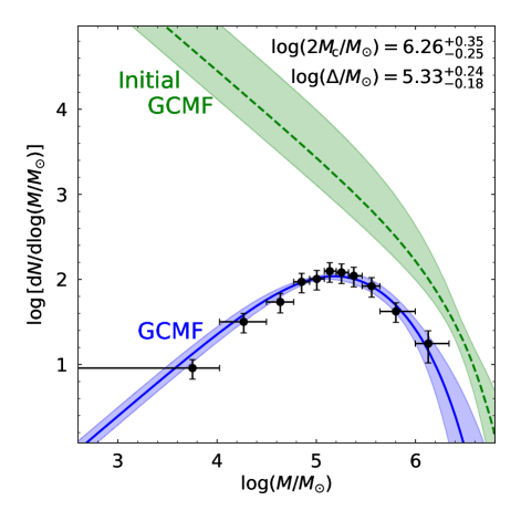
Figure 1: GCMF of 156 Milky Way GCs from the Harris catalogue (black dots with error bars). The blue line shows an evolved Schechter function fit (equation 3). The resulting initial GCMF, corrected for mass loss by stellar evolution (factor of 2) and evaporation ($\Delta$), is shown as a green dashed line. The shaded regions and uncertainties of quoted values indicate the 90% credible intervals. The inferred $K$ value implies that the total mass of the Milky Way GC population was 32.5 times higher initially. Half of this mass reduction is because of stellar mass loss and the remaining factor of 16 is due to evaporation.

II.3 The GC formation rate

Next, we compute the cluster formation rate $\dot{\rho}_{\rm GC}\equiv\dot{\rho}_{\rm GC}(\tau)$, where $\tau$ is lookback time, for a set of model assumptions. We do this in terms of a normalised GC formation rate $R\equiv R(\tau)$, such that $\int_{\infty}^{0}R{\rm d}\tau=1$. In the next section we will derive $R$ from a model for GC formation across cosmic time. For a given present-day $\rho_{\rm GC}$ (equation 2), and no mass loss, the GC formation is then found from $\dot{\rho}_{\rm GC}=\rho_{\rm GC}R$. We now show how $\dot{\rho}_{\rm GC}$ can be easily derived for a population of GCs with a given present-day mass function that have lost mass by stellar evolution and/or escape. Thus, after we determine $\phi_{\rm cl,0}$, we can find $\dot{\rho}_{\rm GC}$ from imposing

$$\dot{\rho}_{\rm GC}=K\rho_{\rm GC}R.$$ (7)

The cluster mass formed per unit volume integrated over all times is

$$\rho_{\rm GC0} =\int_{\infty}^{0}\dot{\rho}_{\rm GC}{\rm d}\tau=K\rho_{\rm GC},$$ (8)

$$=2.4^{+2.3}_{-1.2}\times 10^{16}~{}{M}_{\odot}\,{\rm Gpc}^{3}\ .$$ (9)

The large error bars are because of the uncertainty in $K$ and $\langle\eta\rangle$, and imply that $\rho_{\rm GC0}$ is uncertain by a factor of 2. In the next section we include this uncertainty in the predictions for the merger rate.

III Methodology

The evolution of the BHBs in our cluster models is computed using the fast code cBHBd. While the details of this method are described in Antonini and Gieles (2020), here we give a brief summary of the model philosophy, including the full set of differential equations that are used to compute the secular evolution of the cluster models and the merging BHBs they produce.

III.1 clusterBH

We assume that the cluster consists of two types of members: BHs and all the other members (i.e. other stellar remnants and stars). Each contribute a total mass of $M_{\rm BH}$ and $M_{\star}$, respectively, such that the total cluster mass is $M_{\rm cl}=M_{\star}+M_{\rm BH}$. We assume that after several relaxation time-scales the cluster reaches a state of balanced evolution (Hénon, 1975; Breen and Heggie, 2013), so that the heat generated in the core by the BHBs and the evolution of the cluster global properties are related as (Hénon, 1961; Gieles et al., 2011; Breen and Heggie, 2013):

$$\dot{E}=\zeta\frac{|E|}{t_{\rm rh}},$$ (10)

where $E\simeq-0.2GM_{\rm cl}^{2}/r_{\rm h}$ is the total energy of the cluster, with $M_{\rm cl}$ the total cluster mass and $r_{\rm h}$ the half-mass radius. The constant $\zeta\simeq 0.1$ (Gieles et al., 2011), and $t_{\rm rh}$ is the average relaxation time-scale within $r_{\rm h}$ which is given by (e.g., Spitzer and Hart, 1971)

$$t_{\rm rh}=0.138\sqrt{\frac{M_{\rm cl}r_{\rm h}^{3}}{G}}\frac{1}{\langle m_{\rm all}\rangle\psi\ln\kappa}.$$ (11)

Here $\langle m_{\rm all}\rangle$ is the mean mass of the stars and remnants (initially $\langle m_{\rm all}\rangle=0.638\,M_{\odot}$), and $\ln\kappa$ is the Coulomb logarithm, which varies slowly with $N$, but we fix it to $\ln\kappa=10$. The quantity $\psi$ depends on the mass spectrum within $r_{\rm h}$, for which we adopt the following form:

$$\delta=1+a_{1}{f_{\rm BH}}\ ,$$ (12)

where $f_{\rm BH}=M_{\rm BH}/M_{\rm cl}$ is the fraction of mass in BHs to the total cluster mass and $a_{1}$ is a constant that was determined from a comparison to $N$-body models (see below). We define the start of the balanced evolution as

$$t_{\rm cc}=N_{\rm rh}t_{\rm rh,0}.$$ (13)

Under the above assumptions, the set of coupled ordinary differential equations given below are integrated forward in time to obtain solutions for $M_{\rm BH}(t)$, $M_{\rm cl}(t)$ and $r_{\rm h}(t)$.

The mass loss rate of BHs is coupled to the energy generation rate, which itself is coupled to the total $E$ and $t_{\rm rh}$ of the cluster (equation 10), such that (Breen and Heggie, 2013)

$$\dot{M}_{\rm BH}=\begin{cases}0,&t<t_{\rm cc}{\rm~{}or~{}}M_{\rm BH}=0,\\ \displaystyle-\beta{M_{\rm cl}\over t_{\rm rh}}\ ,&t\geq t_{\rm cc}{\rm~{}and~{}}M_{\rm BH}>0.\end{cases}$$ (14)

The cluster mass loss due to stellar evolution is

$$\dot{M}_{\star,\rm sev}=\begin{cases}0,&t<t_{\rm sev},\\ \displaystyle-\nu{M_{\star}\over t},&t\geq t_{\rm sev},\end{cases}$$ (15)

with $t_{\rm sev}\simeq 2\,\rm Myr$. We include here an additional (mass independent) term which was not present in Antonini and Gieles (2020), and that accounts for cluster evaporation

$$\dot{M}_{\star,\rm ev}=-{\Delta\over\langle t\rangle}\ ,$$ (16)

with $\langle t\rangle\simeq 10\,$Gyr the averaged cluster formation time. The total mass loss rate of the cluster is then

$$\dot{M}=\dot{M}_{\star,\rm sev}+\dot{M}_{\star,\rm ev}+\dot{M}_{\rm BH}\ .$$ (17)

In balanced evolution, the expansion rate of the cluster radius as the result of relaxation is

$$\dot{r}_{\rm h,rlx}=\zeta{r_{\rm h}\over t_{\rm rh}}+2\frac{\dot{M}}{M_{\rm cl}}r_{\rm h}\ .$$ (18)

Before balanced evolution, the cluster radius expands adiabatically as the result of stellar mass loss at a rate

$$\dot{r}_{\rm h,sev}=-{\dot{M}_{\star,\rm sev}\over M_{\rm cl}}r_{\rm h}.$$ (19)

The final expression for the half-mass radius evolution is

$$\dot{r}_{\rm h}=\begin{cases}\dot{r}_{\rm h,sev},&t<t_{\rm cc},\\ \dot{r}_{\rm h,sev}+\dot{r}_{\rm h,rlx},&t\geq t_{\rm cc}.\end{cases}$$ (20)

The remaining parameters were obtained in Antonini and Gieles (2020) by fitting the results of $N$-body simulations: $N_{\rm rh}=3.21$, $\beta=2.80\times 10^{-3}$, $\nu=8.23\times 10^{-2}$ and $a_{1}=1.47\times 10^{2}$.

III.2 BHBdynamics

The initial contraction of the cluster core due to two-body relaxation leads to high central densities of BHs which favor the formation of binaries through three-body processes. The energy produced by the BHBs reverts the contraction process of the core and powers the subsequent expansion of the cluster as described by equation (18). We can then relate the BHB hardening rate to the rate of energy generation

$$\dot{E}_{\rm bin}=-\dot{E}\ ,$$ (21)

where $\dot{E}_{\rm bin}$ is the hardening rate of all core binaries. Equation (21) allows us to couple in a simple way the evolution of the BHBs to the evolution of the cluster model. It is important to stress that the hardening rate equation (21) depends neither on the number of binaries present in the cluster core nor on the exact mechanism leading to their formation.

In order to compute a merger rate and the binary properties from equation (21), we need to further specify the dynamical processes that lead to the hardening and merger of the binaries. We are interested in mergers that occur through (strong) binary-single dynamical encounters in the cluster core (e.g., Gültekin et al., 2004; Samsing, 2018). Thus we consider: (i) mergers that occur in between binary-single encounters while the binary is still bound to its parent cluster (in-cluster inspirals); (ii) mergers that occur during a binary-single (resonant) encounter as two BHs are driven to a short separation such that gravitational wave (GW) radiation will lead to their merger (GW captures); and (iii) mergers that occur after the binary is ejected from its parent cluster. We use BHBdynamics to determine the rate and masses of the BH binary mergers produced by these three dynamical channels.

In balanced evolution, after a binary is ejected or merges a new binary must quickly form to meet the energy demand from the cluster. Under such conditions, the binary formation rate nearly equals the binary ejection rate and it is given therefore by the BH mass ejection rate equation (14) divided by the total mass ejected by each binary

$$\Gamma_{\rm bin} \simeq-\frac{\dot{M}_{\rm BH}}{m_{\rm ej}},$$

where $m_{\rm ej}$ was computed using equation (38) in Antonini and Gieles (2020), and it is approximately a fixed number $m_{\rm ej}\simeq 6m$. The number of BHBs that merge before a time $t$ from the formation of the cluster is (Antonini and Gieles, 2020)

$$\mathcal{N}(<t) =\int_{0}^{t}\Gamma_{\rm bin}\left[{{P}}_{\rm in}+{{P}}_{\rm ej}(t-t^{\prime})\right]{\rm d}t^{\prime},$$ (23)

where $P_{\rm ej}(t-t_{\rm ej})$ is the probability that a binary ejected dynamically from the cluster at a time $t_{\rm ej}$ will merge due to GW emission within a time $t$ from the formation of the cluster, and ${{P}}_{\rm in}$ is the probability that a binary merges inside the cluster. Specifically, ${{P}}_{\rm in}$ is the sum of the probability that that a binary merges through an in-cluster inspiral and the probability of a GW capture. As described in Antonini and Gieles (2020), the probability that a binary merges in between two binary-single interactions is given by integrating the differential merger probability per binary-single encounter over the total number of binary-single interactions experienced by the binary. Similarly, the probability that a binary merges through a GW capture is obtained by dividing each binary-single encounter into 20 intermediate resonant states as in Samsing (2018), and by integrating the differential merger probability per resonant encounter over all encounters experienced by a binary. The merger probabilities are computed by assuming that the eccentricity of the BHBs follows that of a so-called thermal distribution $N(e)\propto e$ (e.g., Heggie, 1975), and their full expressions can be found in Antonini and Gieles (2020). Moreover, when evaluating $P_{\rm ej}$ and $P_{\rm in}$ we set $E_{\rm bin}=-Gm_{1}m_{2}/2a$, with $a$ the binary semi-major axis and $m_{1}$ and $m_{2}$ the mass of the BH components, i.e., we have assumed that only one BHB is responsible for all the heating at any given time. However, because the dependence is weak, e.g. $P_{\rm in}\propto\dot{E}_{\rm bin}^{-2/7}$ (Antonini and Gieles, 2020), and the number of hard binaries is expected to be of order unity in the type of clusters we consider Binney and Tremaine (2008), this simplification is reasonable.

III.3 Black hole mass function and natal kicks

In order to calculate the merger rate through equation (23) we need a physically motivated model for the BH mass function and its time evolution.

We sample 100 stellar progenitor masses from the initial mass-function $\phi_{\star}(m_{\star})\propto m_{\star}^{-2.3}$ (Kroupa, 2001) between $m_{\star,\rm lo}$ and $100M_{\odot}$, with $m_{\star,\rm lo}\simeq 20\,M_{\odot}$ the stellar mass above which a BH forms. The resulting masses of the BHs are then obtained using the fast stellar evolution code SSE (Hurley et al., 2000) which we modified to include up to date prescriptions for stellar wind driven mass loss (Vink et al., 2001), compact-object formation and supernova kicks (Belczynski et al., 2010; Fryer et al., 2012), and we also include prescriptions to account for pulsational-pair instabilities and pair-instability supernovae (Belczynski et al., 2016). The initial mass fraction in BHs is set equal to the total mass in BHs divided by the total mass in stars between $0.1$ and $m_{\star,\rm lo}$ for a Kroupa (2001) initial mass function, and ranges from $f_{\rm bh}\simeq 0.04$ to $0.07$ depending on the metallicity and the adopted prescription for compact-object formation. These mass fractions first increase as the result of stellar evolution mass loss and then they reduce due to the ejection of BHs caused by natal kicks and dynamical ejections. The BH natal kicks are computed using a standard fallback model in which the BHs receive a kick drawn from a Maxwellian distribution with dispersion $\sigma=265\,{\rm km\,s}^{-1}$ (Hobbs et al., 2005), lowered by the fraction of the ejected supernova mass that falls back into the compact-object. The fallback fraction and remnant masses are determined according to the chosen remnant-mass prescription. We adopt here the rapid supernova prescription described in Section 4 of Fryer et al. (2012), in which the explosion is assumed to occur within the first 250ms after bounce. But later in Section IV.2 we also explore other choices for the compact-object formation recipe.

The cluster dynamically processes its BH population such that the mass of the merging BHBs progressively decreases with time because the most massive BHs are the first to reach the cluster core, form hard binaries and merge (e.g., Rodriguez et al., 2016). Assuming that the merger products of BHB mergers are ejected, simulations of dense star clusters also show that the merging BHBs have a distribution of mass-ratio that is strongly peaked around one (e.g., Park et al., 2017). Thus, we assume that the BHs taking part in the dynamical interactions have the same mass, and that at any given time this mass is equal to that of the largest BH in the cluster, i.e., $m_{1}=m_{2}=m_{3}=m_{\rm max}$. The value of $m_{\rm max}$ at a given time, can be easily linked to the time evolution of the total mass in BHs given by clusterBH. For a generic BH mass function $\phi_{\bullet}$, we use the fact that

$$\int_{m_{\rm lo}}^{m_{\rm max}}\phi_{\bullet}m{\rm d}m=M_{\rm BH}\ ,$$ (24)

where the integral in the left hand side is simply the cumulative distribution of BH masses computed with SSE. We then invert numerically this relation to find $m_{\rm max}(M_{\rm BH})$.

III.4 Cluster formation and initial properties

We sample the initial cluster masses from the Schechter mass function equation (5), i.e., we assume that both evaporation and stellar mass loss are important. The values [$\Delta$, $M_{\rm c}$] needed to compute $\phi_{\rm cl,0}$ and $K$ are sampled from their posterior distributions derived in Section II.2.

An important property of balanced evolution is that the value of a cluster half-mass radius today is largely independent of its initial value Hénon (1961); Gieles et al. (2010). It is therefore not possible to infer the initial density of GCs from their properties today. We therefore consider three choices for the initial stellar mass density within the half-mass radius, $\rho_{0}=3M_{0}/(8\pi{r}_{\rm h,0}^{3})$, which we set equal to $\rho_{0}=10^{4}\,M_{\odot}\,{\rm pc}^{-3}$ for our canonical Mod1, and increase(decrease) by a factor 10 in Mod2(Mod3) to explore the effect of initial cluster density.

For the cluster metallicity, we fit a quadratic polynomial to the observed age-metallicity relation for the Milky Way GCs (VandenBerg et al., 2013), to obtain the mean metallicity

$$\log(Z_{\rm mean}/Z_{\odot})\simeq 0.42+0.046\left({t\over{\rm Gyr}}\right)-0.017\left({t\over{\rm Gyr}}\right)^{2}\ .$$ (25)

Given the cluster age, $t$, we then assume a log-normal distribution of metallicity around the mean, with standard deviation $\sigma=0.4$ dex. This takes into account the large spread found in the observed age-metallicity relation. In order to determine the effect of metallicity on our results we will later consider additional models where the cluster metallicity is set to a fixed value.

We obtain the distribution of cluster formation times from the semi-analytical galaxy formation model of El-Badry et al. (2019). The same model has also been used in recent work (e.g., Rodriguez and Loeb, 2018; Samsing et al., 2019), allowing a direct comparison of our results to literature. El-Badry et al. (2019) describe the process of GC formation as resulting from star formation activity in the high-density disks of gas-rich galaxies. Motivated by the results of simulations of molecular cloud collapse, they assume that massive bound clusters form preferentially when the gas surface density exceeds a certain threshold. Applying this Ansatz to a semi-analytic gas model built on dark matter merger trees, they make predictions for the cosmological formation rate of GCs. The resulting cluster formation history peaks at a redshift of $\sim 4$, which is earlier than the peak in the cosmic star formation history (redshift $\sim 2$, Madau and Dickinson (2014)). We sample the formation redshift of our cluster models from the total cosmic cluster formation rate given by the fiducial model of El-Badry et al. (2019) and integrated over all halo masses. This corresponds to the formation rate per comoving volume of their Figure 8 with their parameters $\beta_{\Gamma}=1$ and $\beta_{\eta}=1/3$, where $\beta_{\Gamma}$ sets the dependence of the cluster formation efficiency on surface density, and $\beta_{\eta}$ the dependence of the star formation rate on the halo virial mass. We then normalize the GC formation to unit total number to obtain $R$ (equation 7). Thus, we only sample the cluster formation redshift from the El-Badry et al. (2019) model, while the total cluster formation rate is given by our equation (7). For this model, approximately 25% of the cosmic star formation Madau and Dickinson (2014) is in star clusters at redshifts $\gtrsim 4$ (i.e. before the peak) for $K=32.5$, implying that $K=130$ is an upper limit to ensure that the cluster formation rate is below the star formation rate. This limit corresponds to $2.5\sigma$ in our $K$ distribution and hence it is unlikely to occur. Later, in order to determine the importance of our assumption about the cluster formation history, we will consider another class of models with different values for $\beta_{\Gamma}$ and $\beta_{\eta}$.

Given the initial cluster mass, radius, metallicity, and formation time, the BHB merger rate, $\dot{\mathcal{N}}$, is obtained from cBHBd.

IV binary black hole merger rate

The merger rate density of BHBs at a lookback time $\tau$ is

$$\mathcal{R}(\tau) = \int\int\int{\phi_{\rm cl,0}}(M_{0})R(\tau^{\prime})s(Z)$$ (26)

$$\dot{\mathcal{N}}(\tau^{\prime}-\tau;M_{0},r_{\rm h,0},Z){\rm d}\tau^{\prime}{\rm d}M_{0}{\rm d}Z$$

where $\dot{\mathcal{N}}(t;M_{0},r_{\rm h,0},Z)$ is the BHB merger rate corresponding to a cluster with an initial mass $M_{0}$, half-mass radius $r_{\rm h,0}$ and metallicity $Z$ at a time $t$ after its formation; $R(\tau)$ is the normalized cluster formation rate and $s(Z)$ is the normalized formation rate of clusters with a metallicity $Z$ at a time $\tau$, $\int s(Z;\tau){\rm d}Z=1$, which can be calculated given a model for the time evolution of metallicity, e.g., equation (25).

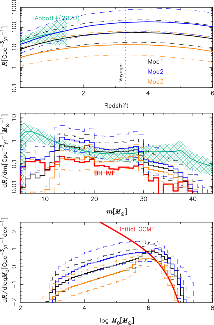
Figure 2: Median of the merger rate distribution (solid lines) for different initial cluster half-mass densities corresponding to Mod1, Mod2 and Mod3 in Table 1. The dashed lines contain $90\%$ of all model realizations (between the $5$ and $95$ percentiles). The upper panel gives the merger rate as a function of redshift. The middle and lower panels show the differential local merger rate as a function of the the primary BH mass and initial cluster mass, respectively. We compare our results to the median (solid), and the $90\%$ credible intervals (hatched regions) inferred from the GWTC-2 catalogue in Abbott et al. (2020). In the middle panel, we have used their ‘Power Law & Peak’ model and the thick-red line gives the BH initial mass function (in arbitrary units). In the lower panel we show the initial GMF (in arbitrary units) four our best fit value $\log(2M_{c}/M_{\odot})=6.26$. Vertical dotted line corresponds to the LIGO Voyager upgrade horizon for $(10+10)~{}M_{\odot}$ BHBs (LIGO Scientific Collaboration and Harms, 2017). The observable horizons of the Einstein telescope (et al., 2010) and the Cosmic Explorer (LIGO Scientific Collaboration and Harms, 2017) extend to the very early Universe and are both to the right of the $x$-axis range in the figure.

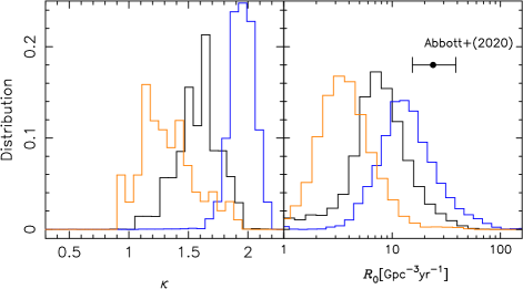
Figure 3: Distribution of the rate parameter $\kappa$, and the local merger rate, $\mathcal{R}_{0}$, for each of the three models of Fig. 2. Colors are as in Fig.2.

Model	Density	Z	Cluster formation	BH masses	Natal	$\dot{M}_{\star,\rm ev}$	$\mathcal{R}_{0}$	$\kappa$	$\mathcal{R}_{0,\rm in-cluster}$
	$M_{\odot}\,{\rm pc}^{-3}$				kicks		[$\rm Gpc^{-3}yr^{-1}$]		[$\rm Gpc^{-3}yr^{-1}$]
Mod1	$10^{4}$	Eq. (25)	$\beta_{\Gamma}=1;~{}\beta_{\eta}=1/3$	Rapid	fallback	Eq.  (16)	$7.2^{+12.7}_{-4.5}$	$1.61^{+0.26}_{-0.37}$	$1.8^{+1.6}_{-1.0}$
Mod2	$10^{5}$	-	-	-	-	-	$12.2^{+32.9}_{-7.9}$	$1.92^{+0.16}_{-0.17}$	$2.0^{+1.7}_{-1.1}$
Mod3	$10^{3}$	-	-	-	-	-	$3.0^{+5.6}_{-1.9}$	$1.23^{+0.53}_{-0.35}$	$1.1^{+1.2}_{-0.6}$
Mod4	$10^{4}$	0.01$\rm Z_{\odot}$	-	-	-	-	$6.8^{+13.6}_{-3.9}$	$1.60^{+0.22}_{-0.33}$	$1.8^{+1.8}_{-1.1}$
Mod5	-	0.1$\rm Z_{\odot}$	-	-	-	-	$7.5^{+16.0}_{-5.3}$	$1.57^{+0.27}_{-0.38}$	$2.0^{+2.0}_{-1.2}$
Mod6	-	$\rm Z_{\odot}$	-	-	-	-	$6.9^{+15.4}_{-3.2}$	$1.51^{+0.30}_{-0.26}$	$2.7^{+2.5}_{-1.7}$
Mod7	-	Eq. (25)	All form at z=3	-	-	-	$7.5^{+15.5}_{-4.5}$	$1.72^{+0.26}_{-0.34}$	$1.8^{+1.8}_{-1.1}$
Mod8	-	-	$\beta_{\Gamma}=0;~{}\beta_{\eta}=1/3$	-	-	-	$7.6^{+16.3}_{-5.1}$	$1.53^{+0.25}_{-0.38}$	$2.1^{+2.5}_{-1.4}$
Mod9	-	-	$\beta_{\Gamma}=1;~{}\beta_{\eta}=1/6$	-	-	-	$6.6^{+13.6}_{-4.6}$	$1.54^{+0.29}_{-0.29}$	$1.8^{+1.8}_{-1.0}$
Mod10	-	-	$\beta_{\Gamma}=1;~{}\beta_{\eta}=1/3$	Belczynski et al. (2002)	-	-	$7.1^{+13.6}_{-4.0}$	$1.68^{+0.22}_{-0.31}$	$1.5^{+1.3}_{-0.9}$
Mod11	-	-	-	Belczynski et al. (2008)	-	-	$7.8^{+16.1}_{-4.8}$	$1.64^{+0.30}_{-0.26}$	$1.7^{+1.5}_{-1.0}$
Mod12	-	-	-	Delayed	-	-	$7.1^{+14.6}_{-4.4}$	$1.58^{+0.27}_{-0.36}$	$1.8^{+1.9}_{-1.0}$
Mod13	-	-	-	Rapid	No kicks	-	$10.0^{+21.4}_{-6.9}$	$1.52^{+0.26}_{-0.31}$	$2.4^{+2.5}_{-1.4}$
Mod14	-	-	-	-	momem.	-	$8.0^{+14.5}_{-6.1}$	$1.50^{+0.31}_{-0.34}$	$2.2^{+2.2}_{-1.3}$
Mod15	-	-	-	-	fallback	0	$2.2^{+1.4}_{-1.4}$	$1.22^{+0.13}_{-0.29}$	$0.9^{+0.2}_{-0.2}$
Mod16	$10^{5}$	0.01$\rm Z_{\odot}$	-	-	-	Eq.  (16)	$12.2^{+29.6}_{-8.0}$	$1.87^{+0.14}_{-0.17}$	$1.9^{+1.9}_{-1.1}$
Mod17	-	0.1$\rm Z_{\odot}$	-	-	-	-	$12.7^{+32.4}_{-8.1}$	$1.93^{+0.12}_{-0.20}$	$2.0^{+1.9}_{-1.2}$
Mod18	-	$\rm Z_{\odot}$	-	-	-	-	$10.3^{+24.5}_{-6.7}$	$2.28^{+0.12}_{-0.35}$	$2.3^{+2.9}_{-1.5}$
Mod19	-	Eq. (25)	All form at z=3	-	-	-	$11.1^{+27.9}_{-7.2}$	$2.10^{+0.03}_{-0.12}$	$1.8^{+1.5}_{-1.2}$
Mod20	-	-	$\beta_{\Gamma}=0;~{}\beta_{\eta}=1/3$	-	-	-	$12.3^{+29.4}_{-8.3}$	$1.91^{+0.19}_{-0.21}$	$2.2^{+2.2}_{-1.3}$
Mod21	-	-	$\beta_{\Gamma}=1;~{}\beta_{\eta}=1/6$	-	-	-	$11.5^{+28.1}_{-7.6}$	$1.90^{+0.10}_{-0.15}$	$1.8^{+1.7}_{-1.1}$
Mod22	-	-	$\beta_{\Gamma}=1;~{}\beta_{\eta}=1/3$	Belczynski et al. (2002)	-	-	$13.1^{+34.0}_{-8.4}$	$1.90^{+0.11}_{-0.16}$	$1.9^{+1.9}_{-1.1}$
Mod23	-	-	-	Belczynski et al. (2008)	-	-	$14.5^{+36.7}_{-8.8}$	$1.88^{+0.13}_{-0.13}$	$2.0^{+1.8}_{-1.2}$
Mod24	-	-	-	Delayed	-	-	$11.8^{+27.3}_{-6.8}$	$1.96^{+0.12}_{-0.19}$	$1.9^{+1.7}_{-1.3}$
Mod25	-	-	-	Rapid	No kicks	-	$18.1^{+36.7}_{-6.1}$	$1.80^{+0.14}_{-0.17}$	$3.1^{+2.9}_{-1.7}$
Mod26	-	-	-	-	momem.	-	$14.2^{+32.6}_{-9.2}$	$1.86^{+0.18}_{-0.20}$	$2.7^{+2.4}_{-1.7}$
Mod27	-	-	-	-	fallback	0	$3.2^{+2.4}_{-2.1}$	$1.87^{+0.10}_{-0.19}$	$1.0^{+0.4}_{-0.4}$
Mod28	$10^{3}$	0.01$\rm Z_{\odot}$	-	-	-	Eq.  (16)	$2.7^{+4.7}_{-1.8}$	$1.30^{+0.49}_{-0.33}$	$1.0^{+0.9}_{-0.6}$
Mod29	-	0.1$\rm Z_{\odot}$	-	-	-	-	$3.4^{+5.8}_{-2.2}$	$1.16^{+0.52}_{-0.27}$	$1.1^{+1.2}_{-0.8}$
Mod30	-	$\rm Z_{\odot}$	-	-	-	-	$3.5^{+7.3}_{-2.5}$	$0.91^{+0.32}_{-0.30}$	$1.4^{+2.0}_{-0.8}$
Mod31	-	Eq. (25)	All form at z=3	-	-	-	$2.9^{+5.2}_{-1.9}$	$1.39^{+0.48}_{-0.35}$	$1.0^{+1.0}_{-0.7}$
Mod32	-	-	$\beta_{\Gamma}=0;~{}\beta_{\eta}=1/3$	-	-	-	$3.3^{+5.9}_{-2.1}$	$1.19^{+0.41}_{-0.35}$	$1.1^{+1.2}_{-0.6}$
Mod33	-	-	$\beta_{\Gamma}=1;~{}\beta_{\eta}=1/6$	-	-	-	$2.9^{+4.0}_{-1.9}$	$1.26^{+0.47}_{-0.38}$	$1.0^{+1.0}_{-0.6}$
Mod34	-	-	$\beta_{\Gamma}=1;~{}\beta_{\eta}=1/3$	Belczynski et al. (2002)	-	-	$2.7^{+4.5}_{-1.6}$	$1.44^{+0.46}_{-0.39}$	$0.9^{+0.8}_{-0.5}$
Mod35	-	-	-	Belczynski et al. (2008)	-	-	$2.9^{+4.9}_{-1.7}$	$1.39^{+0.47}_{-0.33}$	$1.0^{+0.9}_{-0.6}$
Mod36	-	-	-	Delayed	-	-	$2.9^{+5.0}_{-1.9}$	$1.22^{+0.44}_{-0.35}$	$1.0^{+1.0}_{-0.6}$
Mod37	-	-	-	-	No kicks	-	$3.7^{+6.4}_{-2.5}$	$1.32^{+0.46}_{-0.31}$	$1.2^{+1.1}_{-0.7}$
Mod38	-	-	-	-	momem.	-	$2.9^{+3.9}_{-1.8}$	$1.02^{+0.54}_{-0.34}$	$1.1^{+1.0}_{-0.6}$
Mod39	-	-	-	-	fallback	0	$0.8^{+0.6}_{-0.4}$	$0.62^{+0.21}_{-0.30}$	$0.46^{+0.02}_{-0.06}$

Table 1: Model parameters used in the calculations. Here $\beta_{\Gamma}$ and $\beta_{\eta}$ refer to the parameters of the cosmological models in El-Badry et al. (2019) that are used to sample the cluster ages in our simulations. The rightmost three columns give the local merger rate density of BHBs, the rate evolution parameter $\kappa$, and the local merger rate of in-cluster mergers (including GW captures).

In practice, for each model assumption in Table 1 we sample 100 values over the posterior distributions of the parameters $M_{\rm c}$ and $\Delta$ obtained from the MCMC fit to the observed Milky Way GCMF. Then, for each pair [$M_{\rm c}$, $\Delta$], we evolve $N_{\rm cl}=600$ models with masses sampled over a grid of constant logarithmic step size, $\delta\log M/{M}_{\odot}=0.01$, in the range $10^{2}-10^{8}{M}_{\odot}$, and use that:

$$\mathcal{R}(z)\simeq K\rho_{\rm GC}{\sum\limits_{i=1}^{N_{\rm cl}}\dot{\mathcal{N}}(z;M_{0,i})\phi_{\rm cl,0}(M_{0,i})M_{0,i}\over\sum\limits_{i=1}^{N_{\rm cl}}\phi_{\rm cl,0}(M_{0,i})M_{\rm 0,i}^{2}},$$ (27)

where the formation time of each cluster is randomly sampled from the corresponding $R(\tau)$ distribution; we then use equation (25) to compute the mean metallicity, $Z_{\rm mean}$, that corresponds to that formation time, and thus find the cluster metallicity by drawing from a log-normal distribution around $Z_{\rm mean}$. The half-mass radius of the cluster is obtained from the cluster mass given the assumed half-mass density. Note that because each cluster has its own metallicity, each time we generate a new BH population using SSE; the fraction of clusters with $Z<0.1Z_{\odot}$ is $\simeq 84\%$. We also take into account the uncertainty on the mass density of GCs in the Universe, $\rho_{\rm GC}$. We assume that the parameter $\rho_{\rm GC}$ follows a Gaussian distribution with mean $7.3\times 10^{14}M_{\odot}\ \rm Gpc^{-3}$ and $\sigma=2.6\times 10^{14}M_{\odot}\ \rm Gpc^{-3}$. We sample 1000 values from this latter distribution and for each of them we use equation (27) to determine a merger rate estimate for each of the [$M_{\rm c}$, $\Delta$] values, and thus obtain a distribution of merger rate density values.

Because our results turn out to be more sensitive to the cluster initial density than to other parameters, we first focus on Mod1, Mod2 and Mod3 in Table 1. In these models we vary $\rho_{0}$ in a range that is relevant to real globular clusters, while keeping fixed all the other parameters as given in the table. This allows us to bracket a plausible range of values for the local merger rate density and its redshift evolution. In Fig. 2 we plot the median of the merger rate distribution and credible intervals as a function of redshift, and the primary BH mass distribution of binaries merging at redshifts $z<1$ as well as the initial mass distribution of the clusters where these binaries originated.

Fig. 2 shows that the difference between our upper and lower bounds on the comoving BH merger rate density is about a factor $\sim 10$ for any density assumption. This is due to the fact that $\mathcal{R}\propto K$ at a very good approximation, and, as we discussed above, tight constraints on $K$ cannot be placed from the present day Milky Way GCMF. Moreover, rates are not too sensitive to the initial cluster density – two orders of magnitude difference in the initial density leads to a factor of $\sim 5$ variation in the local value of $\mathcal{R}$. From this we conclude that the initial density uncertainty is as important as the unknown initial GCMF.

For each initial GCMF, corresponding to new values of [$M_{\rm c}$, $\Delta$] and $\langle\eta\rangle$, we fit the redshift distribution of the merger rate density at $z<2$ using

$$\mathcal{R}(z)=\mathcal{R}_{0}\left(1+z\right)^{\kappa}\ ,$$ (28)

to derive a distribution of values for the parameters $R_{0}$ and $\kappa$ for each of our three density assumptions. In this analysis we neglect the uncertainties associated to each fit because their standard deviations are much smaller than the variation in the inferred parameters across the different models. The initial parameters for each of the three densities and the corresponding median values and uncertainties (5 and 95 percentiles) of $\mathcal{R}_{0}$ and $\kappa$ are given in Table 1 (Mod1, Mod2 and Mod3). The distributions obtained from this analysis are shown in Fig. 3. The local BH merger rate density from GCs varies in the range $R_{0}\simeq 1$ to $50\rm\,Gpc^{-3}yr^{-1}$. A comparison to the local merger rate inferred from the GW detections, $23.9^{+14.9}_{-8.6}\rm Gpc^{-3}yr^{-1}$ (for their redshift independent results and $19.1^{+16.2}_{-9.0}\,\rm Gpc^{-3}yr^{-1}$ when the merger rate is allowed to evolve with redshift) Abbott et al. (2020), shows that BHBs formed dynamically in GCs are likely to explain a significant fraction of the BHB mergers detected by LIGO-Virgo. Note, however, that if GCs are formed with high densities, $\sim 10^{5}\,M_{\odot}\,{\rm pc}^{-3}$, then our merger rate estimates are consistent with the LIGO-Virgo merger rates within uncertainties. We note that although this high density is preferred to explain the overall rates, the rates in the mass range $13-30\,{M}_{\odot}$ are somewhat better reproduced by Mod1 ($10^{4}\,M_{\odot}\,{\rm pc}^{-3}$, see Fig. 2). Combining the three models together, i.e., assuming a universe in which one third of the clusters form as in Mod1, one third as in Mod2 and the remaining as in Mod3, we find

$$\mathcal{R}_{0}=7.2^{+21.5}_{-5.5}{\rm Gpc^{-3}yr^{-1}};~{}~{}\kappa=1.6^{+0.4}_{-0.6},$$ (29)

where uncertainties refer to the $90\%$ credible intervals.

The middle panel of Fig. 2 shows the primary BH mass distribution normalized to the BH merger rate density in the local Universe ($z<1$). Our models MOD1 and MOD2 reproduce well the shape as well as the normalization of the BH mass function inferred from the GWTC-2 Abbott et al. (2020) in the range $13-30{M}_{\odot}$. The BH mass distribution appears to be sensitive to the initial cluster density, in the sense that higher densities lead to a higher fraction of lower mass BHs among the merging population. It is interesting that the higher density models, Mod1 and Mod2, provide a better match to the inferred BH mass function and the rates. The additional low-mass BHs in high density GCs is due to the higher retention fraction of lower mass BHs in higher density models after a natal kick due to the high escape velocities from these clusters, and to the fact that denser clusters process their BH populations faster, thereby ‘eating’ away their BH mass function more.

Given the number of complex features that can be seen in the BH mass distributions we do not attempt here a parametrization over the full range of BH masses. Moreover, as we will show later in Section IV.2, these distributions are sensitive to the uncertain prescriptions for BH formation, natal kicks and metallicity. We instead consider the mass range $13\,M_{\odot}$ to $30\,M_{\odot}$ where a simple power law model, $dR/dm\propto m^{\alpha}$, does a reasonable job. In this mass range we find $\alpha=0.1^{+0.9}_{-0.5}$ (Mod3), $\alpha=-1.1^{+0.4}_{-0.5}$ (Mod1), and $\alpha=-1.8^{+0.6}_{-0.4}$ (Mod2), where the reported values are the median of the distributions obtained by fitting each of the 100 BH mass distributions corresponding to different [$M_{\rm c}$, $\Delta$], and the uncertainties refer to the $5$ and $95$ percentiles. As before we neglect the uncertainties associated to each fit because their standard errors are much smaller than the variation of $\alpha$ across the different models. By combining the three density models together, we find

$$\alpha=-1.1^{+1.5}_{-1.0}\ .$$ (30)

Negative values of $\alpha$ are preferred, though positive values are also acceptable. The value of the power law index found by us is broadly consistent with the value of $\alpha=-1.58^{+0.82}_{-0.86}$ reported by Abbott et al. (2020) for their low-mass ($<40{M}_{\odot}$) slope of the “Broken Power Law” model. For comparison, the BH initial mass function integrated over all metallicities is shown in the middle panel of Fig. 2. Within the same BH mass range, $m=13\,M_{\odot}$ to $30\,{M}_{\odot}$, the best fit power law model to the initial mass function had a spectral index $\alpha\approx-1.8$. The most striking feature, however, is that all mass distributions in Fig. 2 are strongly depleted at $m\lesssim 15\,M_{\odot}$. The fraction of BHs below this mass decreased by more than one order of magnitude with respect to the BH initial mass function. Due to this, all our models underpredict the number of BHBs at $m\sim 10M_{\odot}$ compared to the mass distribution inferred from the LIGO-Virgo detections. Moreover, we note some features that are common to the three models considered here. All three models show peaks at $m\simeq 13\,M_{\odot}$, $20\,M_{\odot}$ and $30\,M_{\odot}$. Above $m=30\,M_{\odot}$ the BH mass distribution starts to decline rapidly with mass until a break at $m\simeq 38\,M_{\odot}$ above which the decline becomes much steeper. All models show essentially no BHs with mass above $40\,M_{\odot}$ or below $5\,M_{\odot}$. The low merger rate value at $\gtrsim 40\,M_{\odot}$ is a consequence of the stellar mass loss prior to the formation of the BHs because a down-turn above $30\,{M}_{\odot}$ is also seen in the BH IMF and we find it even in models that do not include any prescription for pair instability (Spera et al., 2015). Our pulsational-pair instabilities and pair-instability supernovae prescriptions are taken from (Belczynski et al., 2016), and for the maximum initial stellar mass we considered, $100\,M_{\odot}$, they have little or no effect on the resulting BH masses. Note also that we do not consider hierarchical mergers (Antonini and Rasio, 2016). Their contribution to the merger rate is sensitive to the distribution of BH natal spins, which is poorly constrained. Assuming that BHs are formed with no spin, Rodriguez et al. (2019) finds that $\sim 10\%$ of BHB mergers come from previous mergers; when the BH dimensionless spin parameter is increased above $0.1$, the contribution drops to only a few per cent or less. In addition, in the discussion (Section V.3) we show that with our adopted mass-radius relation, less 2nd generation mergers are expected compared to Rodriguez et al. (2018b). Thus, including hierarchical mergers is not expected to significantly change our integrated merger rate estimates. However, the high mass BHs resulting from multiple mergers can partly fill up the mass distributions above $m\sim 40\,M_{\odot}$ where the merger rates from our models are nearly zero.

The bottom panel of Fig. 2 shows the differential contribution of clusters with different masses to the local merger rate ($z<1$). This contribution increases with cluster mass until about $10^{6}\,M_{\odot}$, above which the rate starts to rapidly decrease because of the exponential truncation of the initial GCMF above $M_{\rm c}$. The contribution of clusters with masses larger than $10^{7}\,M_{\odot}$ or smaller than $10^{3}M_{\odot}$ is negligible. In our models, clusters that have a mass $M_{0}<4\times 10^{5}\,M_{\odot}$ are fully disrupted by the present time. These clusters have been neglected in some previous work (e.g., Rodriguez et al., 2015, 2016; Park et al., 2017; Kremer et al., 2020), but we find that they contribute a significant fraction of the local merger rate: $\approx 0.33$, $0.48$ and $0.30$ for Mod1, Mod2 and Mod3 respectively.

IV.1 In-cluster $vs.$ ejected binaries

The merger of a BHB in our models can occur either after the binary has been ejected dynamically from the cluster, or within the cluster itself. In-cluster mergers are relevant because they can lead to the formation of BHs with mass above the pair-instability gap at $\approx 50\,M_{\odot}$ (Antonini and Rasio, 2016; Rodriguez et al., 2018b; Antonini et al., 2019), and the observational implications of this have been discussed in a number of previous papers, e.g. (Fishbach et al., 2017; Gerosa and Berti, 2017; Kimball et al., 2020). Among all in-cluster mergers, GW captures are also particularly important because a fraction of them are expected to have a finite eccentricity at the moment they first chirp within the the LIGO frequency band above 10 Hz (Antonini et al., 2014; Samsing et al., 2014; Antonini et al., 2016; Samsing, 2018; Rodriguez et al., 2018b). Thus, they could be identified among other binaries due to their unique eccentric signature.

In Fig. 4 we show separately the rate evolution of BH mergers occurring among the ejected binaries, those forming inside the cluster and GW captures, as well as the mass distributions of mergers at $z<1$ and the mass distribution of their parent clusters. While in-cluster mergers dominate the rate density at early times, $z\gtrsim 2$, most of the BHB mergers in the local Universe are produced among the ejected population. The local rate of in-cluster mergers is $\simeq 2\rm\,Gpc^{-3}yr^{-1}$ and that of GW captures is $\simeq 0.4\rm\,Gpc^{-3}yr^{-1}$, with little dependence on the initial density assumed. However, the fractional contribution of in-cluster mergers does depend quite strongly on the cluster initial conditions, in the sense that higher densities lead to lower fractions — for $\rho_{0}=10^{3}M_{\odot}\,{\rm pc}^{-3}$, nearly $40\%$ of the local mergers are formed in-cluster, while for the highest initial densities, $\rho_{0}=10^{5}M_{\odot}\,{\rm pc}^{-3}$, in-cluster mergers only contribute $\simeq 15\%$ of the total. The percentage of all in-cluster mergers that occur through a GW capture is $\approx 20\%$ in the local Universe and increases smoothly with redshift, reaching $\approx 30\%$ near the peak of cluster formation activity. Because an order of unity fraction of gravitational wave captures are expected to have a finite eccentricity ($\gtrsim 0.1$) above 10 Hz frequency, we conclude that eccentric mergers from globular clusters contribute $\lesssim 0.4\rm\,Gpc^{-3}yr^{-1}$ to the merger rate in the local universe. This low rate is consistent with the non detection of eccentric binaries in current searches (LIGO Scientific Collaboration and Virgo Collaboration, 2019c).

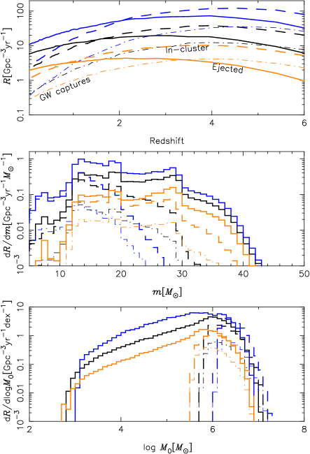
Figure 4: As Fig.2 but we now show separately the median of the merger rate distribution of all in-cluster mergers (dashed lines), only GW captures (dot-dashed lines), and mergers among the ejected binaries (solid lines).

Our models Mod1 and Mod2 show a decrement for the local fraction of in-cluster mergers over previous estimates which bracketed this between $30\%$ and $50\%$ of the total rate (e.g., Rodriguez and Loeb, 2018). This difference arises from the fact that this previous work only considered clusters with mass $\gtrsim 10^{5}M_{\odot}$ for which about half of the overall merger rate is due to in-cluster binaries. However, as shown in Fig. 4, lower mass clusters contribute significantly to the local rate, although the mergers they produce only occur among the ejected population. The reason for this is that their BHs have all been ejected by $z=1$. Thus, including these systems leads to an overall reduction of the contribution of in-cluster mergers and also affects the redshift evolution of the merger rate density.

Fig. 5 shows the distributions of $R_{0}$ and $\kappa$ obtained by fitting equation (28) to the merger rate evolution of in-cluster and ejected binaries separately. The merger rate of in-cluster binaries evolves steeply with redshift, $\kappa\approx 3$, albeit with a large scatter, while for ejected binaries the dependence is much weaker, $\kappa\approx 1$. If, as before, we assign equal probability to each of our density assumptions and fit the total merger rate density of in-cluster binaries using equation (28) we find

$$\mathcal{R}_{\rm 0,in}=1.5^{+1.7}_{-0.9}\,{\rm Gpc^{-3}yr^{-1}};~{}~{}\kappa_{\rm in}=2.3^{+1.3}_{-1.0},$$ (31)

while for ejected binaries

$$\mathcal{R}_{\rm 0,ej}=5.7^{+21.5}_{-4.4}\,{\rm Gpc^{-3}yr^{-1}};~{}~{}\kappa_{\rm ej}=1.2^{+0.4}_{-0.5}.$$ (32)

We now use a simplified analytical model to gain some physical insights on this result.

From equation (23), the merger rate for in-cluster binaries is

$${{\rm d}\mathcal{N}\over{\rm d}t}\Big{|}_{\rm in}=\Gamma_{\rm bin}P_{\rm in}(t)~{},$$ (33)

while for ejected binaries we have

$${{\rm d}\mathcal{N}\over{\rm d}t}\Big{|}_{\rm ej}={{\rm d}\over{\rm d}t}\int_{0}^{t}\Gamma_{\rm bin}P_{\rm ej}(t-t^{\prime}){\rm d}t^{\prime}~{}.$$ (34)

The merger probabilities that enter in the integral equations above can be linked to the evolution of the cluster properties in a simple way under some simplifying assumptions. If we neglect cluster mass loss and that the BHs have a range of masses – both have little effect on the merger rate evolution (see Secion IV.2) – we can write $t_{\rm rh}(t)=t_{\rm rh,0}\left(1+{3\over 2}{\zeta t/t_{\rm rh,0}}\right)$, and $\rho(t)=\rho_{0}\left(1+{3\over 2}{\zeta t/t_{\rm rh,0}}\right)^{-2}$ (Hénon, 1965; Antonini et al., 2019). If $r_{\rm h}\propto t^{2/3}$ and $M=$constant, then $\rho\propto t^{-2}$, $v_{\rm esc}\propto t^{-1/3}$ and therefore $v_{\rm esc}\propto\rho^{1/6}$. Then from Antonini and Gieles (2020) we know $P_{\rm in}\propto v_{\rm esc}^{20/7}$, hence $P_{\rm in}\propto\rho^{10/21}$ (neglecting captures) and $P_{\rm ej}\propto(t-t_{\rm ej})^{2/7}\rho(t)^{8/21}$ Antonini and Gieles (2020). We can then determine the redshift dependence of the merger rate through equations (33) and (34).

At times $t\gg t_{\rm rh,0}/{\zeta}$, for in-cluster binaries we have

$${{\rm d}\mathcal{N}\over{\rm d}t}\Big{|}_{\rm in}\propto(1+z)^{2.9},$$ (35)

where we used that $t(z)\propto(1+z)^{-3/2}$ in order to convert time into redshift. For ejected binaries we have ${{\rm d}\mathcal{N}\over{\rm d}t}\Big{|}_{\rm ej}\propto{t^{-5/7}}$, or

$${{\rm d}\mathcal{N}\over{\rm d}t}\Big{|}_{\rm ej}\propto(1+z)^{1.1}~{}.$$ (36)

Although we have neglected some important ingredients (e.g., mass loss, BH mass function), the expected value of $\kappa$ for the two populations is consistent with the ones found above and, as expected, it is much steeper for in-cluster mergers. This fits in the view that the rate at which the merging BHBs are produced by a cluster is controlled by the relaxation process within the cluster itself, providing a physical interpretation to our results. Moreover it implies that most of the merging BHBs at produced by clusters that are still in the expansion phase.

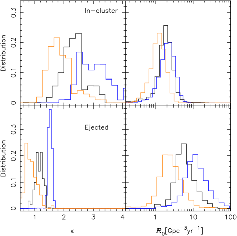
Figure 5: Distribution of the rate parameter $\kappa$, and the local merger rate, $\mathcal{R}_{0}$, for each of the three models of Fig. 2, and for the in-cluster mergers and ejected binary mergers separately. Colors are as in Fig.2.

Figure 6: Example of the BHB merger rate evolution for two cluster masses, and separately for in-cluster and ejected binaries. The middle panels gives the cluster relaxation time, and the lower panels the total BH mass in units of the initial value. Different lines correspond to different initial half-mass density, $\rho_{0}=0.03,\ 0.1,0.3$ and $1\ \times 10^{5}M_{\odot}\,{\rm pc}^{-3}$. The initial density increases with line thickness. Here we set $\Delta=3\times 10^{5}{M}_{\odot}$ and the simulations are terminated either after $13\,$Gyr of evolution or after all BHs have been ejected.

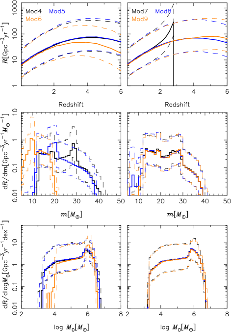
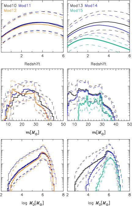
Figure 7: Median of the merger rate distribution (solid lines) and $90\%$ confidence intervals (dashed lines) for the models Mod4 to Mod15 in Table 1 where the initial half-mass density is set to $10^{4}M_{\odot}\,{\rm pc}^{-3}$. Middle panels give the distribution of primary BH masses for mergers at $z<1$. The lower panels show the mass distribution of clusters where these merging binaries were formed.

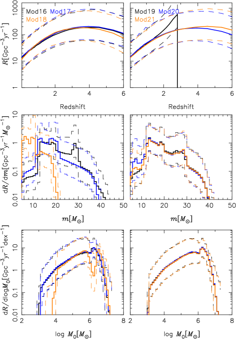
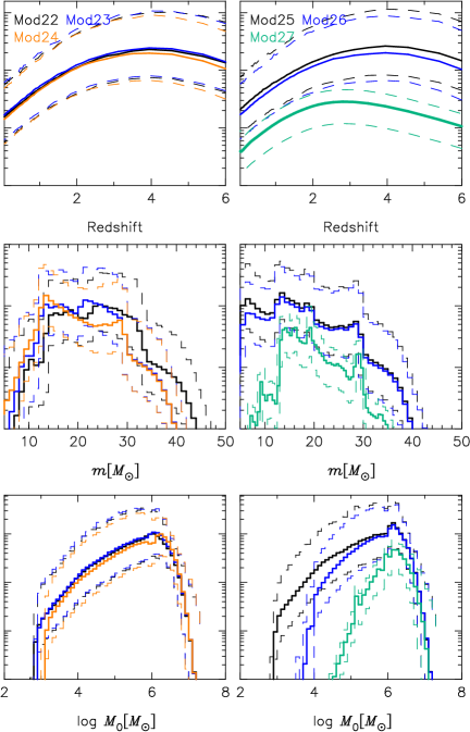
Figure 8: Same as Fig. 7 but for $\rho_{0}=10^{5}M_{\odot}\,{\rm pc}^{-3}$, i.e., Mod16 to Mod27 in Table 1.

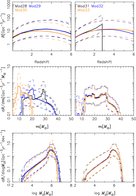
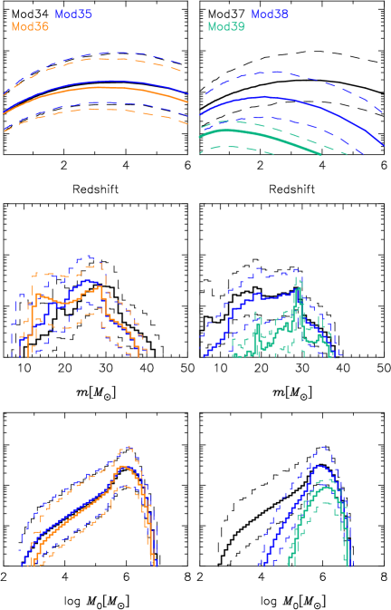
Figure 9: Same as Fig. 7 but for $\rho_{0}=10^{3}M_{\odot}\,{\rm pc}^{-3}$, i.e., Mod28 to Mod39 in Table 1.

Another result of our analysis is that the local rate of in-cluster inspirals and GW captures are nearly independent of the initial density assumed. In general, we find that other model variations also have little effect on the merger rate of in-cluster binaries. This result is because cluster evolution during balanced evolution, i.e. at late stages when in-cluster mergers that we can observe occur, is insensitive to the initial conditions.

Due to the expansion powered by the BHBs, all clusters evolve asymptotically to (approximately) approach the same value of half-mass relaxation time. Hence, after some time, the merger rate of in-cluster binaries must also become approximately the same for all clusters. This concept is illustrated in Fig. 6 where we show the evolution of a set of cluster models with the same mass but different $\rho_{0}$. For $M_{0}=3\times 10^{6}{M}_{\odot}$ (left panels), the BHB merger rate at $\gtrsim 10$ Gyr only varies by a factor of $\sim 2$ between the models, although these were started with widely different densities. The middle panel gives the cluster half-mass relaxation time, which also tends to evolve to the same value for all models. This roughly recovers Hénon’s result that $t/t_{\rm rh}$ increases until $t_{\rm rh}\sim t_{\rm rh,0}/\zeta$, after which $t_{\rm rh}\propto t$ (Gieles et al., 2010).

In the right panel of Fig. 6 we consider the evolution of clusters with an initial lower mass $M_{0}=3\times 10^{5}{M}_{\odot}$. In these models all BHs are ejected at $t\lesssim 5$ Gyr. Thus, their in-cluster binaries do not contribute to the merging population at late times. This explains why in the population models above the local merger rate of in-cluster binaries is widely dominated by high mass systems, $M_{0}\gtrsim 10^{6}{M}_{\odot}$ (e.g., lower panel of Fig. 4). Moreover, the binary merger rate near the end of the simulations shows a larger variation among different models than in the high mass cluster case. This simply reflects the large difference in the cluster density at early times when these binaries were formed and ejected.

IV.2 Dependence on model parameters

In the previous section we consider the merger rate density evolution for three choices of initial cluster density. Here we discuss the results for a larger set of models in which for each of the three density assumptions we vary the prescription for the cluster metallicity, the cosmological cluster formation model, the BH formation mechanism, the BH natal kicks, and the cluster mass loss rate. All the model parameters we considered are listed in Table 1 (Mod4 to Mod39), together with the corresponding values of merger rate evolution parameters and uncertainties. We stress that not all the models analysed here are realistic representations of a globular cluster population. They are nevertheless useful in order to understand the impact of different model parameters on the merger rate evolution and BH mass distribution. Our main message here is that variations in other model assumptions have little effect on the local value of the BHB merger rate density and its redshift evolution. Thus, we conclude this section by presenting the results from an additional set of models where $\rho_{0}$ is varied over a wider range of values than in Section IV to more systematically explore its effect on the BHB merger rate.

Metallicity. In order to explore the dependence of the merger rate on metallicity, we consider models where the clusters all have the same metallicity which we set to $Z=0.01$, 0.1 or $1\times Z_{\odot}$. Since mass loss due to stellar winds is less effective in metal-poor stars, the forming merger remnant mass increases with decreasing metallicity. At Solar metallicity, the mass distribution of the final merger products spans from a few solar masses up to about $30\,M_{\odot}$ and peaks near $10\,M_{\odot}$. At lower metallicity, $Z=0.01$ and 0.1, the distribution of remnant masses is much wider with its maximum at $\sim 50M_{\odot}$. This has an obvious effect on the mass distribution of the merging BHBs as can be seen in Fig. 7, 8 and 9. The value of metallicity affects also what type of clusters make the BH mergers in the local universe, with their mass distribution being skewed towards higher values for Solar metallicities. The important result here, however, is that the evolution of the merger rate density is largely unaffected by the choice of metallicity and its dependence on cluster age. Even in the unrealistic case in which all clusters are formed at Solar metallicity, the merger rate density only starts to deviate significantly from the other models at $z>2$. Such lower merger rate at early times is expected and it is a consequence of the longer $t_{\rm rh}$ due to the lower initial BH mass fraction.

We conclude that a detailed knowledge of the metallicity distribution of GCs and its dependence on time is not necessary in order to determine a BHB merger rate, although it has an important effect on their mass distribution.

Cluster ages. We implemented two additional choices for the parameters in the cosmological model of El-Badry et al. (2019) which determine the distribution of cluster ages: $[\beta_{\Gamma}=1,\ \beta_{\eta}=1/6]$, and $[\beta_{\Gamma}=0,\ \beta_{\eta}=1/3$]. These two models are shown in Fig. 8 of El-Badry et al. (2019). Moreover, we consider an additional case of a burst-like cluster formation history in which all clusters are formed at $z=3$.

From Fig. 7, 8, and 9 we can see that, for a given initial density, our results at $z\lesssim 2$ are also independent of the exact distribution of cluster formation times. Within this redshift, even the oversimplified case in which all clusters form at $z=3$ leads to a merger rate density and BH mass distribution that are consistent with those obtained from the full cosmological models. At $z>2$, however, the redshift evolution of the merger rate is clearly affected with its peak coinciding with the peak of cluster formation activity in each model.

BH formation. We consider three more recipes to computing the BH mass distribution based on different core-collapse/supernova models. We use the delayed model in which the supernova explosion is allowed to occur over a much longer timescale than in the previously employed rapid model (Fryer et al., 2012). We then use the compact-object mass prescriptions from Belczynski et al. (2002) and Belczynski et al. (2008). These two latter models use slightly different recipes for the proto-compact object masses while adopting the same formulae to determine the amount of fallback material. We note that the effect of the BH formation recipe is two folds as it influences both the mass distribution of the BHs as well as their natal kicks. Apart from the effect on the BH mass function, however, there is very little change of the merger rate evolution among the various prescriptions, with the delayed model leading to a slightly lower merger rate at all redshifts than the others.

Natal kicks. Two additional assumptions about the BH natal kicks are explored. In one the BHs are formed with no kick, and in the other the BHs receive the same momentum kick as neutron stars, meaning that their kick velocities are drawn from a Maxwellian distribution with dispersion $\sigma=265\,{\rm km\,s}^{-1}$ (Hobbs et al., 2005) and then reduced by the neutron star to BH mass ratio, $1.4M_{\odot}/m$. Among the model variations considered in this section, the BH natal kick prescription has the largest (but still mild) impact on our results.

The zero kick and the momentum kick prescriptions lead, respectively, to a larger and smaller retention fraction of BHs compared to the fallback prescription (Banerjee et al., 2019). The difference becomes especially important in clusters with initial mass $M_{0}\lesssim 10^{4}M_{\odot}$ because of their lower escape velocities. In these clusters, virtually no BHs are left after the momentum kicks have been imparted, which is reflected in the mass distribution of useful clusters shown in the bottom-right panels of Fig. 7, 8, and 9.

Cluster evaporation. Our mass-independent and orbit-independent mass loss rate for cluster evaporation is certainly a simplified one. To understand its effect on the cluster and BHB evolution, we computed three additional models with exactly the same initial conditions as in Mod1, Mod2 and Mod3 but with $\dot{M}_{\star,\rm ev}=0$. Here we still compute the initial GCMF from equation (5) and use the $[M_{\rm c},\Delta]$ values obtained from the MCMC analysis above, but we do not include any prescription for mass loss when evolving the clusters. Thus, this exercise is only meant to determine the importance of the mass loss effect on the secular evolution of the clusters and the BHBs they produce. We find that in these new models, the local value of the merger rate density and of $\kappa$, as well as the BH mass and progenitor cluster mass distributions are consistent with those found in the models with cluster evaporation included. For the same initial conditions as in Mod1, Mod2 and Mod3 the median values of the local merger rate are $R_{0}=6.9\,\rm Gpc^{-3}yr^{-1}$, $14.1\,\rm Gpc^{-3}yr^{-1}$ and $3.5\,\rm Gpc^{-3}yr^{-1}$, respectively. This shows that cluster evaporation has a small effect on the dynamics of the BHBs.

In our models, however, tidal mass loss must become important at some point, e.g., for high enough $\Delta$, GCs will evaporate before they can produce BHBs. We now quantify how high $\Delta$ needs to be in order to change the BH dynamics significantly. To do this we compare the tidal mass loss timescale, $t_{\rm ev}\equiv M_{0}/|\dot{M}_{\star,\rm ev}|$, to the timescale after which the BHs have been nearly depleted by dynamical ejections, which we define to be $t_{\rm BH}\equiv M_{\rm BH,0}/|\dot{M}_{\rm BH}|$. We should expect that for $t_{\rm BH}<t_{\rm ev}$ most BHBs will have formed already before the cluster mass has changed significantly due to evaporation. This will happen if $\Delta$ is smaller than the critical value

$$\Delta_{\rm c}\simeq{\langle t\rangle\over t_{\rm rh,0}}{\beta\over f_{\rm BH}}M_{0}\ .$$ (37)

For $\rho_{0}=10^{3}M_{\odot}\,{\rm pc}^{-3}$ and $f_{\rm BH}=0.05$, we find $\Delta_{\rm c}\approx 10^{6}M_{\odot}$ independent of the initial cluster mass; for $\rho_{0}=10^{5}M_{\odot}\,{\rm pc}^{-3}$, we have $\Delta_{\rm c}\approx 10^{7}M_{\odot}$. These values are larger than any value of $\Delta$ used in our models (see Fig. 1), explaining the small impact of cluster evaporation on the results.

While the models discussed above show that the impact of cluster evaporation on the BHB dynamics is small, they do not asses its effect on the merger rate. Thus, we consider three new models with $\dot{M}_{\star,\rm ev}=0$ but now use an initial GCMF that only accounts for mass loss due to stellar evolution. If only stellar evolution is included, the initial GCMF that gives rise to the present-day GCMF shown in Fig. 1 becomes:

$$\phi_{\rm cl,0}^{\prime}=0.5A(M_{0}/2+\Delta)^{-2}\exp\left[-(M_{0}/2+\Delta)/M_{\rm c}\right]~{},$$ (38)

and $K\simeq 2$. These new models provide us with a safe lower limit on the BHB merger rate for each density assumption; they are Mod15, Mod27 and Mod39 in Table 1 and Fig. 7, 8 and 9. From these results we see that the merger rate in models without evaporation are about three times smaller than in models where the effect of cluster evaporation is included.

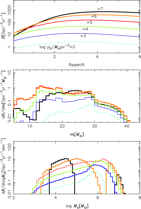
Figure 10: The upper panel shows the median of the merger rate density distribution as a function of redshift; the middle panel gives the distribution of primary BH mass for $z<1$ mergers (median values); and the bottom panel gives the initial mass distribution of clusters contributing to the local mergers (median values). In these calculations we varied the initial cluster density within the indicated range while keeping all the other model parameters the same and as in Mod1 of Table 1.

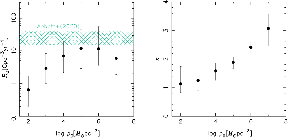
Figure 11: Merger rate parameters as a function of the initial cluster half-mass density for the models of Fig. 10. The black points represent median values, while the lower and upper error bars give the 5 and 95 percentiles of the distributions.

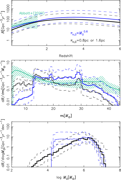
Figure 12: Merger rate evolution, primary BH mass of mergers at $z<1$ and the initial cluster mass distributions where these binaries originated, for a model where half of the clusters have $r_{\rm h,0}=$0.8 pc and the other half have $r_{\rm h,0}$=1.6pc similar to Rodriguez and Loeb (2018) (black lines), and for a model where $r_{\rm h,0}\propto M_{0}^{0.6}$ (blue lines).

Cluster density. The model variations explored above show that for a given initial GCMF, the initial cluster density is clearly the most important parameter for setting the BHB merger rate density and its redshift evolution. Thus, here we perform a more systematic exploration of such dependence by running an additional set of models where the initial cluster density is varied in the range $\rho_{0}=10^{2}M_{\odot}\,{\rm pc}^{-3}$ to $10^{7}M_{\odot}\,{\rm pc}^{-3}$. All other model parameters are set as in Mod1 of Table 1. The results from these additional models are shown in Fig. 10 and Fig. 11.

From Fig. 10 we see that the peak of the merger rate and the redshift at which it occurs in each model increase with $\rho_{0}$, and vary from $\simeq 3\,\rm Gpc^{-3}yr^{-1}$ at $z=3$ for $\rho_{0}=10^{2}\,M_{\odot}\,{\rm pc}^{-3}$, to $\simeq 10^{3}\,\rm Gpc^{-3}yr^{-1}$ at $z=4.5$ for $\rho_{0}=10^{7}\,M_{\odot}\,{\rm pc}^{-3}$. The situation is different, however, when we look at the merger rate in the local Universe. In Fig. 11 we see that the median value of $R_{0}$ has a maximum value of $\simeq 20\,\rm Gpc^{-3}yr^{-1}$ at $\rho_{0}\simeq 10^{5}\,M_{\odot}\,{\rm pc}^{-3}$. This is an important result as it shows that the local BHB merger rate density from the GC channel has a robust upper limit of $\simeq 50\,\rm Gpc^{-3}yr^{-1}$ – the upper error bar estimate for the $\rho_{0}=10^{5}M_{\odot}\,{\rm pc}^{-3}$ model.

The reason why $R_{0}$ decreases with $\rho_{0}$ above a certain density can be understood from the lower panel in Fig. 10. This plot shows the mass distribution of clusters from which the BHBs that merge in the local universe are formed. For initial densities above $10^{5}M_{\odot}\,{\rm pc}^{-3}$ the contribution from clusters in the mass range $10^{5}M_{\odot}\lesssim M_{0}\lesssim 10^{7}M_{\odot}$ gradually decreases as the distribution of cluster masses contributing to the mergers becomes bimodal. Such narrowing of the range of cluster masses that can produce local mergers explains the relatively low merger rate in the higher density models. It also affects the distribution of the primary BH masses as shown in the middle panel of Fig. 10.

We looked into the density dependence of the cluster mass distribution shown in the lower panel of Fig. 10 in more details. We find that the lower mass peak seen in the cluster mass distribution for $\rho_{0}=10^{6}M_{\odot}\,{\rm pc}^{-3}$ and $10^{7}M_{\odot}\,{\rm pc}^{-3}$ is only due to ejected binaries while the higher mass peak is only due to in-cluster mergers. Thus, we can explain the depletion of BHBs that come from intermediate mass clusters by considering the behaviour of the two merging populations when varying $\rho_{0}$. Above a certain initial cluster mass, $v_{\rm esc}$ becomes large enough ($\gtrsim 100{\rm km\,s}^{-1}$) that all BHBs merge inside the cluster. But, because $v_{\rm esc}\propto M^{1/3}\rho^{1/6}$, the value of initial cluster mass that still allows for dynamical ejections to occur goes down as $\rho_{0}$ increases. This explains why the upper end of the mass distribution of clusters that produce mergers from ejected BHBs decreases as $\rho_{0}$ increases. Clusters with an initial mass larger than this value only produce in-cluster mergers. Such clusters, however, can only produce mergers in the local universe if they still contain BHs at the present time. Because the BHs are processed at a rate $t_{\rm BH}^{-1}\propto\sqrt{\rho}/M$, the value of the initial cluster mass above which BHs are still present in the local universe increases with density. This explains why the lower end of the mass distribution of systems that produce in-cluster mergers moves towards larger masses as $\rho_{0}$ increases; clusters with a mass smaller than this value get rid of all their BHs by $z=1$.

Fig. 10 shows that only models in which GCs start with an initially high density $\rho_{0}\gtrsim 10^{4}M_{\odot}\,{\rm pc}^{-3}$ can account for a large fraction of the LIGO-Virgo BHB mergers. Interestingly, these models also give a better fit to the inferred BH mass function above $m\gtrsim 13M_{\odot}$ as seen in Fig 2. Future GW observations will reduce the error bars associated with the merger rate estimates and the BH mass distribution, providing important clues on the the initial densities of GCs.

Finally, we consider two additional model realizations. In one we evolve the same initial conditions as in Rodriguez and Loeb (2018) and Rodriguez et al. (2018a) where half of the clusters have $r_{\rm h,0}=0.8$ pc and the remaining half have $r_{\rm h,0}=$1.6 pc; in the other model, the cluster half-mass radius scales as

$$\log\left({{r}_{\rm h,0}\over{\rm pc}}\right)=-3.56+0.615\log\left({M_{0}\over M_{\odot}}\right)\ .$$ (39)

This latter relation was derived by Gieles et al. (2010) from the results of Hasegan et al. (2005) who fit this Faber-Jackson-like relation to ultra-compact dwarf galaxies (UCDs) and elliptical galaxies. Gieles et al. (2010) derived the initial mass-radius relation correcting for mass loss and expansion by stellar evolution and correcting radii for projection. All the other model parameters are the same as in Mod1 of Table 1. The results of these two new models are shown in Fig. 12. Interestingly, both give a local merger rate, $\simeq 10\,\rm Gpc^{-3}yr^{-1}$, which is similar to the maximum merger rate value we obtained before. Moreover, these results show how the choice of initial half-mass radius relation has a significant effect on both the BH mass and initial cluster mass distributions. For $r_{\rm h,0}\propto M_{0}^{0.6}$, the cluster mass distribution becomes nearly flat so that, roughly speaking, all clusters with initial mass in the range $10^{4}-10^{6}M_{\odot}$ contribute equally to the local merger rate.

V Discussion and conclusions

Our models are based on some assumptions and approximations. These are discussed in the following sections, which also present a more detailed comparison to the literature. We end the paper with a brief summary of our main results.

V.1 Present-day GC mass density

Our value of $\rho_{\rm GC}$ is larger than what was found by Rodriguez et al. (2015): if we adopt their assumption of an average GC mass of $3\times 10^{5}~{}{M}_{\odot}$, we find that equation (2) corresponds to a GC number density of $n_{\rm GC}=2.4~{}{\rm Mpc}^{-3}$, which is $3.3$ times larger than their $n_{\rm GC}=0.72~{}{\rm Mpc}^{-3}$, but similar to the value used in Portegies Zwart and McMillan (2000) and Kremer et al. (2020). Part of this difference is because we adopted a larger value of $\eta$: if we use their mild $M_{\rm h}$-dependent $\eta$ from Harris et al. (2015), we find $n_{\rm GC}=1.50~{}{\rm Mpc}^{-3}$, which corresponds to our lower error bar $\langle\eta\rangle$. However, this is still a factor of 2.1 higher than what was found by Rodriguez et al. (2015). We are not sure what causes this remaining difference, but we note that $n_{\rm GC}=1.50~{}{\rm Mpc}^{-3}$ is about a factor $h^{-2}$ larger than $n_{\rm GC}=0.72~{}{\rm Mpc}^{-3}$ (Carl Rodriguez, private communication).

V.2 Initial GC density in the Universe

To derive $\rho_{\rm GC0}$, a different approach was adopted by Rodriguez and Loeb (2018) and Rodriguez et al. (2018a). They use the total mass density of GCs forming in the semi-analytical galaxy formation model of El-Badry et al. (2019). They approximate the numerical results with analytical functions and find a total $\rho_{\rm GC0}=5.8\times 10^{14}~{}{M}_{\odot}\,{\rm Gpc}^{-3}$, about 15% higher than El-Badry et al. (2019) and 20% lower than our adopted $\rho_{\rm GC}$ (equation 2). They then assume that the initial masses of all GCs were a factor of 2.6 higher (from Choksi et al. (2019)) because of stellar mass loss and evaporation and find that initial mass density of GCs more massive than $10^{5}~{}{M}_{\odot}$ is $\rho_{\rm GC0}(M_{0}>10^{5}~{}{M}_{\odot})\simeq 1.5\times 10^{15}~{}{M}_{\odot}\,{\rm Gpc}^{-3}$. This is a factor of $\sim 4$ higher than found by Rodriguez and Loeb (2018). The reason we find a higher value is that their assumption that the present-day GC density in the Universe is made from GCs with $M_{0}>10^{5}~{}{M}_{\odot}$ that lost (only) a factor of 2.6 in mass implies a mass loss rate that is much lower in our models. In our models the present-day $\rho_{\rm GC0}$ is made of GCs with $M_{0}\gtrsim 4\times 10^{5}~{}{M}_{\odot}$.

In addition, we do consider the contribution to the merger rate of lower mass GCs with $M_{0}<10^{5}~{}{M}_{\odot}$. We Use cBHBd to evolve the same initial conditions as in Rodriguez and Loeb (2018) and Rodriguez et al. (2018a) where half of the clusters have $r_{\rm h,0}=0.8$ pc and the remaining half have $r_{\rm h,0}=$1.6pc but extended the initial GCMF down to $M_{\rm lo}=100M_{\odot}$ (see Fig. 12). We find that $\simeq 10\%$ of the local mergers come from GCs with $M_{0}<10^{5}~{}{M}_{\odot}$, and therefore conclude that for the exact same initial GCMF, our models would lead to a local merger rate that is still $\simeq 4$ times that found in Rodriguez and Loeb (2018) and Rodriguez et al. (2018a). Our Schechter mass is $M_{\rm c}\simeq 2\times 10^{6}M_{\odot}$, so we compare to the results from Rodriguez and Loeb (2018) for mass functions with $M_{\rm c}=(2.5-5)\times 10^{6}M_{\odot}$. For these, the rates in Rodriguez and Loeb (2018) are $5$ to $10\rm Gpc^{-3}yr^{-1}$. The median of the merger rate distribution computed from our models is $10\rm Gpc^{-3}yr^{-1}$. Rodriguez and Loeb (2018) use a fit to the results of a set of Monte Carlo simulations to determine the number of mergers produced by a cluster as a function of time. Because these fitting formulae are not public, it is currently difficult to establish the reason why our rates are only 1 to 2 times, and not 4 times, those in Rodriguez and Loeb (2018). We note in passing that we compared our models to the number of mergers from the two examples shown in Fig. 2B of Rodriguez and Loeb (2018) and found very good agreement.

V.3 O-star ejections and IMBH formation

Our cBHBd model makes the simplifying assumption that all BHs are in place when the cluster forms. Because the typical timescale of GC evolution (i.e. 100 Myr - Gyr) is much longer than the timescale of BH formation (i.e. 10 Myr), this is fine in most cases. However, for very dense, low-mass clusters, the relaxation time is so short that O-stars are ejected as ‘runaway stars’ before they form BHs Poveda et al. (1967); Fujii and Portegies Zwart (2011). As a result, the initial BH fraction is lower in these clusters than what we assume in our models, possibly affecting the merger rate and properties of the mergers. To quantify this, we use the fact that the dynamical process that ejects O-stars is the same as the one that ejects BHs at a later stage. We therefore adopt clusterBH and replace the BH population by a massive star population between $10-100\,M_{\odot}$, with a logarithmic slope of $-2.3$, and a mass fraction of 18%, as appropriate for a Kroupa IMF. We then determine for a grid of initial cluster masses and half-mass radii the maximum mass of massive stars that form BHs inside the cluster. In Fig. 13 we show contours for $20\,M_{\odot}$ (the minimum mass of an O-star to produce a BH), $35\,M_{\odot}$ (approximately half of the mass in BHs is produced by stars more massive than this) and $100\,M_{\odot}$ (the upper limit of our IMF). We also overplot the 3 initial cluster densities adopted in the previous section. From this we see that clusters with $M_{0}\lesssim 10^{4}\,M_{\odot}$ are affected by O-star ejections, which affects about half of the mass in the initial GCMF. However, these low-mass GCs are only responsible for $\sim 15\%$ of the mergers. The fraction of clusters for which more than half of the BH mass is ejected is only a few per cent. Clusters that produce runaways, will have fewer massive BHs, leading to a slightly higher merger rate of slightly less massive BHs. This effect is small, but would lead to a slightly steeper BH mass function especially for the densest models. However, we conclude that runaway stars do not significantly affect our results and that the effect is probably smaller than other uncertainties in our model.

Another process that is not included in cBHBd is repeated mergers of BHs. After a merger, the BH merger remnant receives a general relativistic momentum kick of several 100 km/s, and if this is smaller than the escape velocity from the center of the cluster, it can be involved in subsequent mergers Antonini and Rasio (2016); Rodriguez et al. (2018b, 2019) possibly forming an intermediate-mass BH (IMBH) Antonini et al. (2019). This can only occur for an initial escape velocity $\gtrsim 300\,$km/s and in Fig. 13 we show that only in our densest ($\gtrsim 10^{5}\,{M}_{\odot}/{\rm pc}^{3}$), most massive ($\gtrsim 10^{7}\,{M}_{\odot}$) models this could happen. Ignoring the effect of IMBH formation via dry BH mergers is therefore not affecting our results. Although the formation of IMBHs through repeated mergers is unlikely, we note that hierarchical mergers can still contribute to the BH merger rate. As discussed above, hierarchical mergers represent only ten percent or less of the total number of BHB mergers expected from GCs (Rodriguez et al., 2018b, 2019). Thus, they will not affect significantly our integrated merger rate estimates. On the other hand, second-generation mergers can produce BHs with a mass higher than predicted by stellar evolution alone, broadening the BH mass distributions we derived and populating them above $\sim 40M_{\odot}$.

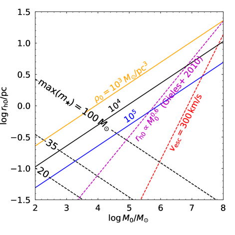
Figure 13: GC initial mass-radius diagram showing the 3 initial cluster densities adopted in this work with dashed lines. The magenta, full line shows the initial mass-radius relation that describes the most massive GCs ($\gtrsim 10^{6}\,{M}_{\odot}$) and ultra-compact dwarf galaxies ($\gtrsim 10^{7}\,{M}_{\odot}$) Hasegan et al. (2005); Gieles et al. (2010). Full lines show the maximum mass of O-stars that form BHs inside the cluster. Clusters with $M\lesssim 10^{4}\,{M}_{\odot}$ will eject some O-stars before they become BHs, and these clusters will therefore have slightly lower BHB mergers than in our model. The red, full line shows an initial escape velocity of 300 km/s, which is the minimum escape velocity required for IMBH formation to occur Antonini et al. (2019). This process is not playing a role in our adopted initial conditions.

V.4 Cluster mass loss and initial GCMF

Our models adopt a constant mass loss for all clusters of $\Delta\simeq 2\times 10^{5}\,{M}_{\odot}$. This is what is required to evolve the initial GCMF with a power-law slope of $-2$ at low-masses to the peaked GCMF of old GCs, but it is inconsistent with some studies of GC evolution. Firstly, $N$-body simulations of tidally limited clusters show that $\dot{M}\propto M^{1/3}$ Baumgardt and Makino (2003), rather than $\dot{M}\propto M^{0}$. Including this mass dependence in $\dot{M}$ and maintaining the constraint that all GCs formed with the same Universal initial mass function, implies that clusters need to lose more mass for the turn-over in the GCMF to move to $2\times 10^{5}\,{M}_{\odot}$ Gieles (2009), resulting in a twice as large value of $K\simeq 64$ Kruijssen and Portegies Zwart (2009) as we found for a mass independent $\dot{M}$. Secondly, the models of Baumgardt and Makino (2003) show that $\Delta$ for a typical Milky Way GC is smaller and depends on the apocenter and eccentricity of the Galactic orbit. For the median Galactocentric distance of Miky Way GCs ($\sim 5\,$kpc) and an age of 10 Gyr, these models find $\Delta\simeq 4\times 10^{4}\,{M}_{\odot}$, i.e. a factor of 5 smaller than what we assumed. These simulations considered the secular evolution of clusters in a static tidal field and therefore underestimate mass loss of clusters if additional disruption processes are important. For example, interactions with massive gas clouds in the early evolution (first Gyr) can be disruptive Spitzer (1958); Gieles et al. (2006), have a similar mass dependence as relaxation driven evaporation in a static tidal field Gieles and Renaud (2016) and lead to a turn over in the GCMF Elmegreen (2010); Kruijssen (2015). If this is the cause for the value of $\Delta$, than $|\dot{M}|$ is much higher in the early evolution, which would affect the resulting merger rate. Because the relaxation time decreases if the mass reduces, including this type of mass evolution will lead to a higher merger rate than in our models with an $\dot{M}$ that is constant in time. The models of Baumgardt and Makino (2003) also do not contain BHs and it has been shown that retaining a BH population significantly increases the escape rate of stars Giersz et al. (2019); Wang (2020). The BH population can increase $|\dot{M}|$ by an order magnitude (Gieles et al., in prep), especially towards the end of the evolution. This implies a relatively low(high) $|\dot{M}|$($t_{\rm rh}$) in the early evolution compared to our models, leading to a reduction of the merger rate. In addition, for $\dot{M}\propto M^{\gamma}$, with $\gamma<0$, the required $K$ to get the turn-over at the right mass is lower than for $\gamma=0$. If BHs are responsible for the value of $\Delta$, our merger rates could therefore also be slightly overestimated for this reason. However, we do not expect this effect to be important for dense clusters ($\gtrsim 10^{4}\,{M}_{\odot}/{\rm pc}^{3}$) because their BHB mergers are produced when the clusters are still unaffected by the Galactic tides. We plan to include the effect of relaxation driven escape in a tidal field in a future version of cBHBd  to address this issue.

Finally, we have assumed that all GC masses are drawn from an initial GCMF that is constrained by the shape of the Milky Way GCs. Although the present-day GCMF is remarkably universal across galaxies, variations in the inferred $M_{\rm c}$ and $\Delta$ values of a factor of $\sim 5$ are found across GC populations in galaxies in the Virgo cluster Jordán et al. (2007). Higher $M_{\rm c}$ and lower $\Delta$ values are found in brighter galaxies. Although variations in $M_{\rm c}$ and $\Delta$ are partially captured by the uncertainties in $M_{\rm c}$ and $\Delta$, this accounts only for up to a factor of $\sim 2$. We may therefore under-populate the most massive clusters.

V.5 Primordial binaries

The effect of binaries that form in the star formation process and undergo stellar evolution in the first stages of cluster evolution has not been discussed so far. We argue here that primordial binaries have a negligible effect on the merger rate and the distribution of the BH masses we derived. Because of Hénon principle, the energy generation rate by binaries is determined by the relaxation process in the cluster as a whole. Whether dynamically active binaries form in three-body encounters from single BHs, or in encounters involving BHBs that formed from primordial binaries will therefore result in a central binary with the same properties. However, primordial binaries might affect the initial BH mass function due to binary evolution processes. But, because BHB mergers from primordial binaries in GCs are a subdominant population at low redshifts (see Fig. 2 in Rodriguez et al., 2015), the effect on the local BHB mass distribution is also expected to be small.

V.6 Conclusions

In this paper we have considered the dynamical formation of BHB mergers in GCs. Using our new population synthesis code cBHBd we have evolved a large number of models covering a much wider set of initial conditions than explored in the literature. This allowed us to place robust error bars on the merger rate and mass distributions of the merging BHBs. We find that the GC channel produces BHB mergers in the local universe at a rate of $7.2^{+21.5}_{-5.5}\,\rm Gpc^{-3}yr^{-1}$, where the error bars are mostly set by the unknown initial GC mass function and initial cluster density. By comparing to the merger rate inferred by LIGO-Virgo, our results imply that a model in which most of the detected mergers come from GCs is consistent with current constraints. This would require, however, that GCs form with half-mass densities larger than $\gtrsim 10^{4}M_{\odot}\,{\rm pc}^{-3}$, and suppression of other formation mechanisms. All our models show a drop in the merger rate of binary with primary BH mass outside the range $\simeq 13-30M_{\odot}$, for which there is no evidence in the gravitational wave data. This might suggest that another mechanism is responsible for the production of these sources.

Our results have a number of implications for the formation of BHB mergers and GCs. The dependence of the merger rate and BHB properties (e.g., eccentricity, mass) on the model parameters suggests that a direct comparison to the gravitational wave data will allow us to place constraints on the initial conditions of GCs and their evolution. Our models will also help to understand other uncertain parameters that control the formation of BHs and their natal kicks. While these latter parameters have little effect on the merger rate, they have a significantly impact on the masses of the merging BHBs. Thus, useful constraints could be placed once the number of gravitational wave detections will be large enough to to allow for a statistically significant comparison to the inferred BH mass function.

In the future, we plan to consider other type of clusters such as open and nuclear star clusters which are also believed to be efficient factories of gravitational wave sources (Ziosi et al., 2014; Antonini and Rasio, 2016; Di Carlo et al., 2019; Rastello et al., 2019; Antonini et al., 2019). The study of these systems will require us to add additional physics to cBHBd.

VI Acknowledgements

We thank the internal referee of the LVC, Michela Mapelli, for her suggestions, which helped us improve this work. MG thanks Duncan Forbes for helpful discussions on the relation between halo mass and GC population mass. We thank the referee for their constructive comments that helped to improved the paper. FA acknowledges support from a Rutherford fellowship (ST/P00492X/1) from the Science and Technology Facilities Council. We acknowledge the support of the Supercomputing Wales project, which is part-funded by the European Regional Development Fund (ERDF) via Welsh Government.

References

- LIGO Scientific Collaboration (2015) LIGO Scientific Collaboration, Classical and Quantum Gravity 32, 074001 (2015), arXiv:1411.4547 [gr-qc] .
- Virgo Collaboration (2015) Virgo Collaboration, Classical and Quantum Gravity 32, 024001 (2015), arXiv:1408.3978 [gr-qc] .
- Abbott et al. (2016a) B. P. Abbott, R. Abbott, T. D. Abbott, M. R. Abernathy, F. Acernese, K. Ackley, C. Adams, T. Adams, P. Addesso, and R. X. Adhikari, Phys. Rev. Lett. 116, 061102 (2016a), arXiv:1602.03837 [gr-qc] .
- Abbott et al. (2016b) B. P. Abbott, R. Abbott, T. D. Abbott, M. R. Abernathy, F. Acernese, K. Ackley, C. Adams, T. Adams, P. Addesso, and R. X. Adhikari, Physical Review X 6, 041015 (2016b), arXiv:1606.04856 [gr-qc] .
- LIGO Scientific Collaboration and Virgo Collaboration (2019a) LIGO Scientific Collaboration and Virgo Collaboration, The Astrophysical Journal Letters 882, L24 (2019a), arXiv:1811.12940 [astro-ph.HE] .
- Abbott et al. (2019) B. P. Abbott, R. Abbott, T. D. Abbott, S. Abraham, F. Acernese, K. Ackley, C. Adams, R. X. Adhikari, V. B. Adya, C. Affeldt, and et al., Physical Review X 9, 031040 (2019), arXiv:1811.12907 [astro-ph.HE] .
- LIGO Scientific Collaboration and Virgo Collaboration (2019b) LIGO Scientific Collaboration and Virgo Collaboration, Phys. Rev. D 100, 064064 (2019b), arXiv:1907.09384 [astro-ph.HE] .
- LIGO Scientific Collaboration and Virgo Collaboration (2020a) LIGO Scientific Collaboration and Virgo Collaboration, The Astrophysical Journal Letters 896, L44 (2020a), arXiv:2006.12611 [astro-ph.HE] .
- The LIGO Scientific Collaboration and the Virgo Collaboration (2020) The LIGO Scientific Collaboration and the Virgo Collaboration, arXiv e-prints , arXiv:2004.08342 (2020), arXiv:2004.08342 [astro-ph.HE] .
- LIGO Scientific Collaboration and Virgo Collaboration (2020b) LIGO Scientific Collaboration and Virgo Collaboration, Phys. Rev. Lett. 125, 101102 (2020b), arXiv:2009.01075 [gr-qc] .
- Abbott et al. (020a) R. Abbott et al., (2020a), arXiv:2010.14527 [gr-qc] .
- Abbott et al. (2020) R. Abbott et al. (LIGO Scientific, Virgo), (2020), arXiv:2010.14533 [astro-ph.HE] .
- Sigurdsson and Hernquist (1993) S. Sigurdsson and L. Hernquist, Nature 364, 423 (1993).
- Kulkarni et al. (1993) S. R. Kulkarni, P. Hut, and S. J. McMillan, Nature 364, 421 (1993).
- Portegies Zwart and McMillan (2000) S. F. Portegies Zwart and S. L. W. McMillan, The Astrophysical Journal Letters 528, L17 (2000), astro-ph/9910061 .
- Banerjee et al. (2010) S. Banerjee, H. Baumgardt, and P. Kroupa, Monthly Notices of the Royal Astronomical Society 402, 371 (2010).
- Downing et al. (2011) J. M. B. Downing, M. J. Benacquista, M. Giersz, and R. Spurzem, Monthly Notices of the Royal Astronomical Society , no (2011).
- Rodriguez et al. (2015) C. L. Rodriguez, M. Morscher, B. Pattabiraman, S. Chatterjee, C.-J. Haster, and F. A. Rasio, Physical Review Letters 115, 051101 (2015).
- Askar et al. (2017) A. Askar, M. Szkudlarek, D. Gondek-Rosińska, M. Giersz, and T. Bulik, MNRAS 464, L36 (2017), arXiv:1608.02520 [astro-ph.HE] .
- Park et al. (2017) D. Park, C. Kim, H. M. Lee, Y.-B. Bae, and K. Belczynski, MNRAS 469, 4665 (2017), arXiv:1703.01568 [astro-ph.HE] .
- Samsing et al. (2018) J. Samsing, A. Askar, and M. Giersz, Astrophys. J. 855, 124 (2018), arXiv:1712.06186 [astro-ph.HE] .
- Zevin et al. (2019) M. Zevin, J. Samsing, C. Rodriguez, C.-J. Haster, and E. Ramirez-Ruiz, Astrophys. J. 871, 91 (2019), arXiv:1810.00901 [astro-ph.HE] .
- Kremer et al. (2020) K. Kremer, C. S. Ye, N. Z. Rui, N. C. Weatherford, S. Chatterjee, G. Fragione, C. L. Rodriguez, M. Spera, and F. A. Rasio, The Astrophysical Journal Supplement Series 247, 48 (2020), arXiv:1911.00018 [astro-ph.HE] .
- Fragione and Kocsis (2018) G. Fragione and B. Kocsis, Phys. Rev. Lett. 121, 161103 (2018), arXiv:1806.02351 [astro-ph.GA] .
- Gnedin and Ostriker (1997) O. Y. Gnedin and J. P. Ostriker, Astrophys. J. 474, 223 (1997).
- Vesperini and Heggie (1997) E. Vesperini and D. C. Heggie, MNRAS 289, 898 (1997), arXiv:astro-ph/9705073 [astro-ph] .
- Fall and Zhang (2001) S. M. Fall and Q. Zhang, Astrophys. J. 561, 751 (2001), arXiv:astro-ph/0107298 [astro-ph] .
- Baumgardt and Makino (2003) H. Baumgardt and J. Makino, Monthly Notices of the Royal Astronomical Society 340, 227 (2003).
- Gieles and Baumgardt (2008) M. Gieles and H. Baumgardt, MNRAS 389, L28 (2008), arXiv:0806.2327 .
- Jordán et al. (2007) A. Jordán, D. E. McLaughlin, P. Côté, L. Ferrarese, E. W. Peng, S. Mei, D. Villegas, D. Merritt, J. L. Tonry, and M. J. West, The Astrophysical Journal Supplement Series 171, 101 (2007), arXiv:astro-ph/0702496 .
- Rodriguez and Loeb (2018) C. L. Rodriguez and A. Loeb, Astrophys. J. 866, L5 (2018), arXiv:1809.01152 [astro-ph.HE] .
- Chatterjee et al. (2017) S. Chatterjee, C. L. Rodriguez, and F. A. Rasio, Astrophys. J. 834, 68 (2017), arXiv:1603.00884 .
- Gieles et al. (2010) M. Gieles, H. Baumgardt, D. C. Heggie, and H. J. G. L. M. Lamers, MNRAS 408, L16 (2010), arXiv:1007.2333 [astro-ph.GA] .
- Antonini and Gieles (2020) F. Antonini and M. Gieles, MNRAS 492, 2936 (2020), arXiv:1906.11855 [astro-ph.HE] .
- Rodriguez et al. (2016) C. L. Rodriguez, S. Chatterjee, and F. A. Rasio, Phys. Rev. D 93, 084029 (2016), arXiv:1602.02444 [astro-ph.HE] .
- Spitler and Forbes (2009) L. R. Spitler and D. A. Forbes, MNRAS 392, L1 (2009), arXiv:0809.5057 [astro-ph] .
- Georgiev et al. (2010) I. Y. Georgiev, T. H. Puzia, P. Goudfrooij, and M. Hilker, MNRAS 406, 1967 (2010), arXiv:1004.2039 [astro-ph.CO] .
- Harris et al. (2013) W. E. Harris, G. L. H. Harris, and M. Alessi, The Astrophysical Journal 772, 82 (2013).
- Harris et al. (2015) W. E. Harris, G. L. Harris, and M. J. Hudson, Astrophys. J. 806, 36 (2015), arXiv:1504.03199 [astro-ph.GA] .
- Harris et al. (2017) W. E. Harris, J. P. Blakeslee, and G. L. H. Harris, Astrophys. J. 836, 67 (2017), arXiv:1701.04845 [astro-ph.GA] .
- Harris (1996) W. E. Harris, Astronomical Journal 112, 1487 (1996).
- Harris (2010) W. E. Harris, arXiv:1012.3224 (2010), arXiv:1012.3224 [astro-ph.GA] .
- Watkins et al. (2019) L. L. Watkins, R. P. van der Marel, S. T. Sohn, and N. W. Evans, Astrophys. J. 873, 118 (2019), arXiv:1804.11348 [astro-ph.GA] .
- Tinker et al. (2010) J. L. Tinker, B. E. Robertson, A. V. Kravtsov, A. Klypin, M. S. Warren, G. Yepes, and S. Gottlöber, The Astrophysical Journal 724, 878 (2010).
- Murray et al. (2013) S. G. Murray, C. Power, and A. S. G. Robotham, Astronomy and Computing 3, 23 (2013), arXiv:1306.6721 [astro-ph.CO] .
- Planck Collaboration (2018) Planck Collaboration, arXiv:1807.06209 , arXiv:1807.06209 (2018), arXiv:1807.06209 [astro-ph.CO] .
- Forbes et al. (2018) D. A. Forbes, J. I. Read, M. Gieles, and M. L. M. Collins, MNRAS 481, 5592 (2018), arXiv:1809.07831 [astro-ph.GA] .
- Schechter (1976) P. Schechter, “An analytic expression for the luminosity function for galaxies.” (1976).
- Portegies Zwart et al. (2010) S. F. Portegies Zwart, S. L. McMillan, and M. Gieles, Annual Review of Astronomy and Astrophysics 48, 431 (2010).
- Bromm and Clarke (2002) V. Bromm and C. J. Clarke, The Astrophysical Journal Letters 566, L1 (2002), arXiv:astro-ph/0201066 .
- Baumgardt and Makino (2003) H. Baumgardt and J. Makino, MNRAS 340, 227 (2003), arXiv:astro-ph/0211471 [astro-ph] .
- Ostriker et al. (1972) J. P. Ostriker, L. J. Spitzer, and R. A. Chevalier, The Astrophysical Journal Letters 176, L51 (1972).
- Gnedin et al. (1999) O. Y. Gnedin, L. Hernquist, and J. P. Ostriker, Astrophys. J. 514, 109 (1999).
- Spitzer (1958) L. J. Spitzer, Astrophys. J. 127, 17 (1958).
- Gieles et al. (2006) M. Gieles, S. F. Portegies Zwart, H. Baumgardt, E. Athanassoula, H. J. G. L. M. Lamers, M. Sipior, and J. Leenaarts, MNRAS 371, 793 (2006), astro-ph/0606451 .
- Elmegreen (2010) B. G. Elmegreen, The Astrophysical Journal Letters 712, L184 (2010), arXiv:1003.0798 .
- Kruijssen (2015) J. M. D. Kruijssen, Monthly Notices of the Royal Astronomical Society 454, 1658 (2015).
- Gieles and Renaud (2016) M. Gieles and F. Renaud, MNRAS 463, L103 (2016), arXiv:1605.05940 .
- Hénon (1961) M. Hénon, Annales d’Astrophysique 24, 369 (1961).
- Foreman-Mackey et al. (2012) D. Foreman-Mackey, D. W. Hogg, D. Lang, and J. Goodman, arXiv preprint arXiv: … 125, 1 (2012).
- Ha\textcommabelowsegan et al. (2005) M. Ha\textcommabelowsegan, A. Jordán, P. Côté, S. G. Djorgovski, D. E. McLaughlin, J. P. Blakeslee, S. Mei, M. J. West, E. W. Peng, and L. Ferrarese, Astrophys. J. 627, 203 (2005), arXiv:astro-ph/0503566 [astro-ph] .
- Rodriguez et al. (2018a) C. L. Rodriguez, P. Amaro-Seoane, S. Chatterjee, K. Kremer, F. A. Rasio, J. Samsing, C. S. Ye, and M. Zevin, Phys. Rev. D 98, 123005 (2018a), arXiv:1811.04926 [astro-ph.HE] .
- Hénon (1975) M. Hénon, in Dynamics of the Solar Systems, IAU Symposium, Vol. 69, edited by A. Hayli (1975) p. 133.
- Breen and Heggie (2013) P. G. Breen and D. C. Heggie, Monthly Notices of the Royal Astronomical Society 432, 2779 (2013).
- Gieles et al. (2011) M. Gieles, D. C. Heggie, and H. Zhao, MNRAS 413, 2509 (2011), arXiv:1101.1821 [astro-ph.GA] .
- Spitzer and Hart (1971) L. Spitzer, Jr. and M. H. Hart, Astrophys. J. 164, 399 (1971).
- Gültekin et al. (2004) K. Gültekin, M. C. Miller, and D. P. Hamilton, Astrophys. J. 616, 221 (2004), astro-ph/0402532 .
- Samsing (2018) J. Samsing, Phys. Rev. D 97, 103014 (2018), arXiv:1711.07452 [astro-ph.HE] .
- Heggie (1975) D. C. Heggie, Monthly Notices of the Royal Astronomical Society 173, 729 (1975).
- Binney and Tremaine (2008) J. Binney and S. Tremaine, Galactic Dynamics: Second Edition, by James Binney and Scott Tremaine. ISBN 978-0-691-13026-2 (HB). Published by Princeton University Press, Princeton, NJ USA, 2008. (Princeton University Press, 2008).
- Kroupa (2001) P. Kroupa, MNRAS 322, 231 (2001).
- Hurley et al. (2000) J. R. Hurley, O. R. Pols, and C. A. Tout, MNRAS 315, 543 (2000), arXiv:astro-ph/0001295 .
- Vink et al. (2001) J. S. Vink, A. de Koter, and H. J. G. L. M. Lamers, Astronomy and Astrophysics 369, 574 (2001).
- Belczynski et al. (2010) K. Belczynski, T. Bulik, C. L. Fryer, A. Ruiter, F. Valsecchi, J. S. Vink, and J. R. Hurley, Astrophys. J. 714, 1217 (2010), arXiv:0904.2784 [astro-ph.SR] .
- Fryer et al. (2012) C. L. Fryer, K. Belczynski, G. Wiktorowicz, M. Dominik, V. Kalogera, and D. E. Holz, The Astrophysical Journal 749, 91 (2012).
- Belczynski et al. (2016) K. Belczynski, A. Heger, W. Gladysz, A. J. Ruiter, S. Woosley, G. Wiktorowicz, H. Y. Chen, T. Bulik, R. O’Shaughnessy, D. E. Holz, C. L. Fryer, and E. Berti, Astronomy & Astrophysics 594, A97 (2016), arXiv:1607.03116 [astro-ph.HE] .
- Hobbs et al. (2005) G. Hobbs, D. R. Lorimer, A. G. Lyne, and M. Kramer, Monthly Notices of the Royal Astronomical Society 360, 974 (2005).
- Rodriguez et al. (2016) C. L. Rodriguez, S. Chatterjee, and F. A. Rasio, Physical Review D 93, 084029 (2016).
- VandenBerg et al. (2013) D. A. VandenBerg, K. Brogaard, R. Leaman, and L. Casagrande, The Astrophysical Journal 775, 134 (2013).
- El-Badry et al. (2019) K. El-Badry, E. Quataert, D. R. Weisz, N. Choksi, and M. Boylan-Kolchin, MNRAS 482, 4528 (2019), arXiv:1805.03652 [astro-ph.GA] .
- Samsing et al. (2019) J. Samsing, T. Venumadhav, L. Dai, I. Martinez, A. Batta, M. Lopez, E. Ramirez-Ruiz, and K. Kremer, Phys. Rev. D 100, 043009 (2019), arXiv:1901.02889 [astro-ph.HE] .
- Madau and Dickinson (2014) P. Madau and M. Dickinson, Annu Rev Astron Astr 52, 415 (2014), arXiv:1403.0007 [astro-ph.CO] .
- LIGO Scientific Collaboration and Harms (2017) LIGO Scientific Collaboration and J. Harms, Classical and Quantum Gravity 34, 044001 (2017), arXiv:1607.08697 [astro-ph.IM] .
- et al. (2010) M. P. et al., Classical and Quantum Gravity 27, 194002 (2010).
- Belczynski et al. (2002) K. Belczynski, V. Kalogera, and T. Bulik, The Astrophysical Journal 572, 407 (2002).
- Belczynski et al. (2008) K. Belczynski, V. Kalogera, F. A. Rasio, R. E. Taam, A. Zezas, T. Bulik, T. J. Maccarone, and N. Ivanova, The Astrophysical Journal Supplement Series 174, 223 (2008).
- Spera et al. (2015) M. Spera, M. Mapelli, and A. Bressan, Monthly Notices of the Royal Astronomical Society 451, 4086 (2015).
- Antonini and Rasio (2016) F. Antonini and F. A. Rasio, Astrophys. J. 831, 187 (2016), arXiv:1606.04889 [astro-ph.HE] .
- Rodriguez et al. (2019) C. L. Rodriguez, M. Zevin, P. Amaro-Seoane, S. Chatterjee, K. Kremer, F. A. Rasio, and C. S. Ye, Phys. Rev. D 100, 043027 (2019), arXiv:1906.10260 [astro-ph.HE] .
- Rodriguez et al. (2018b) C. L. Rodriguez, P. Amaro-Seoane, S. Chatterjee, and F. A. Rasio, Phys. Rev. Lett. 120, 151101 (2018b), arXiv:1712.04937 [astro-ph.HE] .
- Antonini et al. (2019) F. Antonini, M. Gieles, and A. Gualandris, MNRAS 486, 5008 (2019), arXiv:1811.03640 [astro-ph.HE] .
- Fishbach et al. (2017) M. Fishbach, D. E. Holz, and B. Farr, The Astrophysical Journal Letters 840, L24 (2017), arXiv:1703.06869 [astro-ph.HE] .
- Gerosa and Berti (2017) D. Gerosa and E. Berti, Phys. Rev. D 95, 124046 (2017), arXiv:1703.06223 [gr-qc] .
- Kimball et al. (2020) C. Kimball, C. Talbot, C. P. L. Berry, M. Carney, M. Zevin, E. Thrane, and V. Kalogera, arXiv e-prints , arXiv:2005.00023 (2020), arXiv:2005.00023 [astro-ph.HE] .
- Antonini et al. (2014) F. Antonini, N. Murray, and S. Mikkola, The Astrophysical Journal 781, 45 (2014).
- Samsing et al. (2014) J. Samsing, M. MacLeod, and E. Ramirez-Ruiz, The Astrophysical Journal 784, 71 (2014).
- Antonini et al. (2016) F. Antonini, S. Chatterjee, C. L. Rodriguez, M. Morscher, B. Pattabiraman, V. Kalogera, and F. A. Rasio, The Astrophysical Journal 816, 65 (2016).
- LIGO Scientific Collaboration and Virgo Collaboration (2019c) LIGO Scientific Collaboration and Virgo Collaboration, Astrophys. J. 883, 149 (2019c).
- Hénon (1965) M. Hénon, Annales d’Astrophysique 28, 62 (1965).
- Banerjee et al. (2019) S. Banerjee, K. Belczynski, C. L. Fryer, P. Berczik, J. R. Hurley, R. Spurzem, and L. Wang, arXiv e-prints , arXiv:1902.07718 (2019), arXiv:1902.07718 [astro-ph.SR] .
- Choksi et al. (2019) N. Choksi, M. Volonteri, M. Colpi, O. Y. Gnedin, and H. Li, Astrophys. J. 873, 100 (2019), arXiv:1809.01164 [astro-ph.GA] .
- Poveda et al. (1967) A. Poveda, J. Ruiz, and C. Allen, Boletin de los Observatorios Tonantzintla y Tacubaya 4, 86 (1967).
- Fujii and Portegies Zwart (2011) M. S. Fujii and S. Portegies Zwart, Science 334, 1380 (2011), arXiv:1111.3644 [astro-ph.GA] .
- Gieles (2009) M. Gieles, MNRAS 394, 2113 (2009), 0901.0830 .
- Kruijssen and Portegies Zwart (2009) J. M. D. Kruijssen and S. F. Portegies Zwart, The Astrophysical Journal Letters 698, L158 (2009), arXiv:0905.3744 [astro-ph.GA] .
- Kruijssen (2015) J. M. D. Kruijssen, MNRAS 454, 1658 (2015), arXiv:1509.02163 .
- Giersz et al. (2019) M. Giersz, A. Askar, L. Wang, A. Hypki, A. Leveque, and R. Spurzem, MNRAS 487, 2412 (2019), arXiv:1904.01227 [astro-ph.GA] .
- Wang (2020) L. Wang, MNRAS 491, 2413 (2020), arXiv:1911.05077 [astro-ph.GA] .
- Ziosi et al. (2014) B. M. Ziosi, M. Mapelli, M. Branchesi, and G. Tormen, Monthly Notices of the Royal Astronomical Society 441, 3703 (2014).
- Di Carlo et al. (2019) U. N. Di Carlo, N. Giacobbo, M. Mapelli, M. Pasquato, M. Spera, L. Wang, and F. Haardt, MNRAS 487, 2947 (2019), arXiv:1901.00863 [astro-ph.HE] .
- Rastello et al. (2019) S. Rastello, P. Amaro-Seoane, M. Arca-Sedda, R. Capuzzo-Dolcetta, G. Fragione, and I. Tosta e Melo, MNRAS 483, 1233 (2019), arXiv:1811.10628 [astro-ph.GA] .