Qibo: a framework for quantum simulation with hardware acceleration

Abstract

We present Qibo, a new open-source software for fast evaluation of quantum circuits and adiabatic evolution which takes full advantage of hardware accelerators. The growing interest in quantum computing and the recent developments of quantum hardware devices motivates the development of new advanced computational tools focused on performance and usage simplicity. In this work we introduce a new quantum simulation framework that enables developers to delegate all complicated aspects of hardware or platform implementation to the library so they can focus on the problem and quantum algorithms at hand. This software is designed from scratch with simulation performance, code simplicity and user friendly interface as target goals. It takes advantage of hardware acceleration such as multi-threading CPU, single GPU and multi-GPU devices.

PROGRAM SUMMARY

Program Title: Qibo

Program URL: https://github.com/qiboteam/qibo

Licensing provisions: Apache-2.0

Programming language: Python, C/C++

Nature of the problem: Simulation of quantum circuits and adiabatic evolution requires implementation of efficient linear algebra operations. The simulation cost in terms of memory and computing time is exponential with the number of qubits.

Solution method: Implementation of algorithms for the simulation of quantum circuits and adiabatic evolution using the dataflow graph infrastructure provided by the TensorFlow framework in combination with custom operators. Extension of the algorithm to take advantage of multi-threading CPU, single GPU and multi-GPU setups.

1 Introduction and motivation

During the last decade, we have observed an impressive fast development of quantum computing hardware. Nowadays, quantum processing units (QPUs) are based on two approaches, the quantum circuit and quantum logic gate-based model processors as implemented by Google [1], IBM [2], Rigetti [3] or Intel [4], and the annealing quantum processors such as D-Wave [5, 6]. The development of these devices and the achievement of quantum advantage [7] are clear indicators that a technological revolution in computing will occur in the coming years.

The quantum computing paradigm is based on the hardware implementation of qubits, the quantum analogue to bits, which are used as the representation of quantum states. Currently, quantum computer manufacturers provide systems containing up to dozens of qubits for circuit-based quantum processors, while annealing quantum processors can reach thousands of qubits. Thanks to the qubits representation it is possible to implement quantum algorithms based on different approaches such as the quantum Fourier transform [8], amplitude amplification and estimation [9], search for elements in unstructured databases [10, 11], BQP-complete problems [12], and hybrid quantum-classical models [13]. These algorithms are the possible key solution for different types of problems such as optimization [14] and prime factorization [15]. However, in several cases, an algorithm’s implementation may require systems with large number of qubits, thus even if in principle we can simulate the behaviour of quantum hardware devices using quantum mechanics on classical computers, the computational performance becomes quickly unpractical due to the exponential scaling of memory and time.

The quantum computer simulation on classical hardware is still quite relevant in the current research stage, because thanks to simulation, researchers can prototype and study a priori the behaviour of new algorithms on quantum hardware. In terms of simulation techniques, there are at least three common approaches such as the linear algebra implementation of the quantum-mechanical wave-function propagation, the Feynman path-integral formulation of quantum mechanics [16, 17] and tensor networks [18].

The simulation of circuit-based quantum processors is already implemented by several research collaborations and companies. Some notable examples of simulation software which are based on linear algebra approach are Cirq [19] and TensorFlow Quantum (TFQ) [20] from Google, Qiskit from IBM Q [21], PyQuil from Rigetti [22], Intel-QS (qHipster) from Intel [23] , QCGPU [24] and Qulacs [25], among others [26, 27, 28, 29, 30, 31, 32, 33, 34, 35, 36, 37, 38, 39, 40, 41, 42, 43, 44, 45]. While the simulation techniques and hardware-specific configurations are well defined for each simulation software, despite the availability of recent implementations based on Field Programmable Gate Arrays (FPGAs) [46, 47], there are no simulation tools that can take full advantage of hardware acceleration in single and double precision computations, through a simple interface which allows the user to switch from multithreading CPU, single GPU, and distributed multi-GPU/CPU setups. On the other hand, from the point of view of quantum annealing computation, in particular adiabatic quantum computation, there are several examples of applications in the literature [48, 49, 50]. However, classical simulation of adiabatic evolution algorithms used by this computational paradigm are not systematically implemented in public libraries.

Module	Description
models	Qibo models (details in Table 2).
gates	Quantum gates that can be added to Qibo circuit.
callbacks	Calculation of physical quantities during circuit simulation.
hamiltonians	Hamiltonian objects supporting matrix operations and Trotter decomposition.
solvers	Integration methods used for time evolution.

Table 1: Modules supported by Qibo 0.1.0.

Qibo model	Description
Circuit	Basic circuit model containing gates and/or measurements.
DistributedCircuit	Circuit that can be executed on multiple devices.
QFT	Circuit implementing the Quantum Fourier Transform.
VQE	Variational Quantum Eigensolver. Supports optimization of the variational parameters.
QAOA	Quantum Approximate Optimization Algorithm. Supports optimization of the variational parameters.
StateEvolution	Unitary time evolution of quantum states under a Hamiltonian.
AdiabaticEvolution	Adiabatic time evolution of quantum states. Supports optimization of the scheduling function.

Table 2: qibo.models implemented in Qibo 0.1.0.

In this work, we present the Qibo framework [51] for quantum simulation with hardware acceleration (code available at [52]). Qibo is designed with three target goals: a simple application programming interface (API) for quantum circuit design and adiabatic quantum computation, a high-performance simulation engine based on hardware acceleration tools, with particular emphasis on multithreading CPU, single GPU and multi-GPU setups, and finally, a clean design pattern to include classical/quantum hybrid algorithms. In general the inclusion of hardware acceleration support requires a good knowledge of multiple programming languages such as C/C++ and Python, and hardware specific frameworks such as CUDA [53], OpenCL [54] and OpenMP [55]. However, given that the knowledge of each of these tools could be a strong technical barrier for users interested in custom circuit designs, and subsequently, the simulation of new quantum and hybrid algorithms, Qibo proposes a framework build on top of the TensorFlow [56] library which reduces the effort required by the user. Tables 1 and 2 provide an overview of the basic modules and models that are implemented in the current version of Qibo 0.1.0.

The Qibo framework will become the entry point in terms of API and simulation engine for the middleware of a new quantum experimental research collaboration coordinated by [57, 58].

The paper is organized as follows. In Sec. 2 we present the technical aspects of the Qibo framework, highlighting the code structure, algorithms, and features. In Sec. 3, we show benchmarking results comparing the Qibo simulation performance with other popular libraries. The Sec. 4 is dedicated to applications provided by Qibo as examples. Finally, in Sec. 5 we present our conclusion and future development direction.

2 Technical implementation

In this section we present the technical structure of Qibo, an open-source library for quantum circuit definition and simulation which takes advantage of hardware accelerators such as GPUs.

2.1 Acceleration paradigm

Hardware acceleration combines the flexibility of general-purpose processors, such as CPUs, with the efficiency of fully customized hardware, such as GPUs, increasing efficiency by orders of magnitude.

In particular, hardware accelerators such as GPUs with a large number of cores and memory are getting popular thanks to their great efficiency in deep learning applications. Open-source frameworks such as TensorFlow simplify the development strategy by reducing the required hardware knowledge from the developer’s point of view.

In this context, Qibo implements quantum circuit simulation using TensorFlow primitives and custom operators together with job scheduling for multi-GPU synchronization. The choice of TensorFlow as the backend development framework for Qibo is motivated by its simple mechanism to write efficient Python code which can be distributed to hardware accelerators without complicated installation procedures.

2.2 Code structure

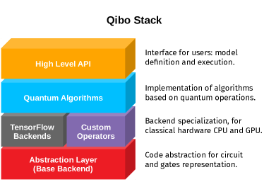
Figure 1: Schematic view of the Qibo structure design.

In Fig. 1 we show a schematic representation of the code structure. The ground layer represents the base abstraction layer, where the circuit structure and gates are defined. On top of the abstraction layer, we specialize the simulation system using TensorFlow and numpy [59] primitives. The backend layers are required in order to build quantum algorithms such as the Variation Quantum Eigensolver (VQE) [60], perform measurement shots, etc. These algorithms are implemented in such a way that there is no direct dependency on the backend specialization. Furthermore, several models delivered by Qibo, such as VQE, QAOA and adiabatic evolution, require minimization techniques provided by external libraries, in particular TensorFlow for stochastic gradient descent, Scipy [61] for quasi-Newton methods and CMA-ES [62] for evolutionary optimization. Finally, we provide the entry point for code usage through a simple high-level API in Python.

2.3 Backends and algorithms

Qibo simulates the behavior of quantum circuits using dense complex state vectors $\psi(\sigma_{1},\sigma_{2},\dots,\sigma_{N})\in\mathbb{C}$ in the computational basis where $\sigma_{i}\in\{0,1\}$ and $N$ is the total number of qubits in the circuit. The main usage scheme is the following:

⬇

import numpy as np

from qibo import models, gates

\par# create a circuit for N=3 qubits

circuit = models.Circuit(3)

\par# add some gates in the circuit

circuit.add([gates.H(0), gates.X(1)])

circuit.add(gates.RX(0, theta=np.pi/6))

\par# execute the circuit and obtain the

# final state as a tf.Tensor

final_state = circuit()

where qibo.models.Circuit is the core Qibo object and holds a queue of quantum gates. Each gate corresponds to a matrix $G(\boldsymbol{\tau},\boldsymbol{\tau^{\prime}})=G(\tau_{1},\dots,\tau_{N_{\mathrm{targets}}},\tau_{1}^{\prime},\dots,\tau_{N_{\mathrm{targets}}}^{\prime})$ and acts on the state vector via the matrix multiplication

$$\psi^{\prime}(\sigma_{1},\ldots,\sigma_{N})=\sum_{\boldsymbol{\tau^{\prime}}}G(\boldsymbol{\tau},\boldsymbol{\tau^{\prime}})\psi(\sigma_{1},\ldots,\boldsymbol{\tau^{\prime}},\ldots,\sigma_{N})$$ (1)

where the sum runs over qubits targeted by the gate.

When a circuit is executed, the state vector is transformed by applying matrix multiplications for every gate in the queue. By default, the result of circuit execution is the final state vector $\psi^{\prime}$ after all gates have been applied. If measurement gates are used then the returned result contains measurement samples following the distribution corresponding to the final state vector. The computational difficulty in this calculation is that the dimension of $\psi$ increases exponentially with the number of qubits $N$ in the circuit.

Qibo provides three different backends for implementing the matrix multiplication of Eq. (1), all based on TensorFlow 2. There are two backends (defaulteinsum and matmuleinsum) based on TensorFlow native operations and the custom backend that uses custom C++ operators. Table 3 provides a feature comparison between the different backends. The default backend is custom, however the user can easily switch to a different backend using the qibo.set_backend() method.

In the two TensorFlow backends the state vector $\psi$ is stored as a rank-$N$ TensorFlow tensor (tf.Tensor) and gate matrices as rank-$2N_{\mathrm{targets}}$ tensors. In the defaultein-
sum backend, matrix multiplication is implemented using the tf.einsum method, while in the matmuleinsum backend using tf.matmul. In the latter case, the state has to be transposed and reshaped to $(2^{N_{\mathrm{targets}}},2^{N-N_{\mathrm{targets}}})$ shape using the tf.transpose and tf.reshape operations, as tf.matmul by definition supports only matrix (rank-2 tensor) multiplication. The motivation to have both implementations is justified by performance: the defaulteinsum backend is faster on GPUs while the matmuleinsum is more efficient on CPU. The main advantage of using backends based on native TensorFlow primitives is that support for backpropagation is inherited automatically. This may be useful when gradient-descent-based minimization schemes are used to optimize variational quantum circuits. On the other hand, TensorFlow operations create multiple state vector copies, increasing execution time and memory usage, particularly for large qubit numbers.

In order to increase simulation performance and reduce memory usage, we implemented custom TensorFlow operators that perform Eq. (1). The state is stored as a vector with $2^{N}$ components, and the indices of its components that should be updated during the matrix multiplication are calculated by the custom operators during each gate application. This allows all gate applications to happen in-place without requiring any copies of the state vector, thus reducing memory requirements to the minimum ($2^{N}$ complex numbers for $N$ qubits). Furthermore, the sparsity of some common quantum gates is exploited to increase performance. For example, the $Z$ gate is applied by flipping the sign of only half of the state components while the rest remain unaffected. Custom operators are coded using C++ and support multi-threading via TensorFlow’s thread pool implementation. An additional CUDA implementation is provided for all operators to allow execution on GPU.

	Native	Custom
Backend names	defaulteinsum matmuleinsum	custom
GPU support	✓	✓
Distributed computation		✓
In-place state updates		✓
Measurements	✓	✓
Controlled gates	✓	✓
Density matrices / noise	✓
Callbacks	✓	✓
Gate fusion	✓	✓
Backpropagation	✓

Table 3: Features support for each calculation backend.

2.4 Circuit simulation features

Qibo provides several features aiming to make the simulation of quantum circuits for research purposes easier. In this section, we describe some of these features.

2.4.1 Controlled gates

All Qibo gates can be controlled by an arbitrary number of qubits. Both in the native TensorFlow and custom backends, these gates are applied using the proper indexing of the state vector, avoiding the creation of large gate matrices.

2.4.2 Measurements

Qibo’s measuring mechanism works by sampling the final state vector once all gates of a circuit are applied. Sampling is handled by the tf.random.categorical method. A flexible measurement API is provided, which allows the user to view measurement results in binary or decimal format and as raw measurement samples or frequency dictionaries. It is also possible to group multiple qubits in the same register and perform collective measurements. Note that no density matrix is computed at this step. The final result is a trace-out of the outcome probability in unmeasured qubits.

2.4.3 Density matrices and noise

Native TensorFlow backends can simulate density matrices in addition to state vectors. This allows the simulation of noisy circuits using the channels that are provided as qibo.gates. By default Qibo uses state vectors for simulation. However, it switches automatically to density matrices if a channel is found in the circuit or if the user uses a density matrix as the initial state of a circuit execution. Density matrices are not yet implemented in the custom backend but will be included in future releases.

2.4.4 Callbacks

The callback functions allow the user to perform calculations on intermediate state vectors during a circuit execution. A callback example which is implemented in Qibo is entanglement entropy. This allows the user to track how entanglement changes as the state is propagated through the circuit’s gates. Other callbacks implemented in Qibo include the callbacks.Energy which calculates the energy (expectation value of a Hamiltonian) of a state or callbacks.Gap which calculates the gap of the adiabatic evolution Hamiltonian (we refer to Sec. 2.6 for more details).

2.4.5 Gate fusion

In some cases, particularly for large qubit numbers, it is more efficient to fuse several gates by multiplying their respective unitary matrices and multiply the resulting matrix to the state vector, instead of applying the original gates one-by-one. Qibo provides a simple method (circuit.fuse()) to fuse circuit gates up to a two-qubit $4\times 4$ matrix. Additionally, the VariationalLayer gate is provided for efficient simulation of variational circuits that consist of alternating layers between one-qubit rotations and two-qubit entangling gates. For more details on this we refer to Sec. 3.2.

2.5 Distributed computation

Qibo allows execution of circuits on multiple devices with focus on systems with multiple GPU configurations. As demonstrated in Sec. 3, GPUs are much faster than a typical CPU for circuit simulation, however, they are limited by their internal memory. A typical high-end GPU nowadays has 12-16GB of memory, allowing simulation of up to 29 qubits (30 qubits with single precision numbers) using Qibo’s custom backend. For larger qubits, the user has to use a CPU with sufficient random-access memory (RAM) size or rely on distributed configurations.

Qibo provides a simple API to distribute large circuits to multiple devices. For example, a circuit can be executed on multiple GPUs by passing an accelerators dictionary when creating the corresponding qibo.models.Circuit object, as:

⬇

from qibo.models import Circuit

circuit = Circuit(

nqubits=30,

accelerators={”/GPU:0”: 1, ”/GPU:1”: 1}

)

Dictionary keys define which devices will be used and the values the number of times each device will be used. Note that a single device can be used more than once to increase the number of “logical” devices. For example, a single GPU can be reused multiple times to exceed the limit of 29 qubits, making the distributed implementation useful even for systems with a single GPU.

Device re-usability is allowed by exploiting the system’s RAM. The full state vector is stored in RAM while parts of it are transferred to the available GPUs to perform the matrix multiplications. This state partition to pieces is inspired by techniques used in multi-node quantum circuit simulation [63, 64]. More specifically, if $N_{\mathrm{devices}}$ are available, the state is partitioned by selecting $\log_{2}N_{\mathrm{devices}}$ qubits (called global qubits [65]) and indexing according to their binary values. For example, if $N_{\mathrm{devices}}=2$ and the first qubit is selected as the global qubit, the state of size $2^{N}$ is partitioned to two pieces $\psi(0,\sigma_{2},\dots,\sigma_{N})$ and $\psi(1,\sigma_{2},\dots,\sigma_{N})$ of size $2^{N-1}$. Gates targeting local (non-global) qubits are directly applied by performing the corresponding matrix multiplication on all logical devices. Gates targeting global qubits cannot be applied without communication between devices. The scheme that we currently follow to apply such gates is to move their targets to local qubits by adding SWAP gates between global and local qubits. These SWAP gates are applied on CPU, where the full state vector is available. All gates between SWAPs target local qubits and are grouped and applied together to minimize the CPU-GPU communication.

If logical devices correspond to distinct physical devices, the matrix multiplications are parallelized among physical devices using joblib [66].

In terms of memory, the distributed implementation described above is restricted only by the total amount of RAM available for the system’s CPU and not the GPU memory. The main bottleneck is related to CPU-GPU communication, and therefore the performance depends on the number of SWAP gates required to move all gates’ targets to local qubits. This number depends on the circuit structure. As presented in the practical examples of Sec. 3, a multi-GPU configuration can provide significant speed-up compared to using only the CPU.

2.6 Time evolution

In addition to the circuit simulation presented in the previous sections, Qibo can be used to simulate a unitary time evolution of quantum states. Given an initial state vector $\left|\psi_{0}\right\rangle$ and an evolution Hamiltonian $H$, the goal is to find the state $\left|\psi(T)\right\rangle$ after time $T$, so that the time-dependent Schrödinger equation

$$i\partial_{t}\left|\psi(t)\right\rangle=H\left|\psi(t)\right\rangle$$ (2)

is satisfied. Note that the Hamiltonian may have explicit time dependence.

An application of time evolution relevant to quantum computation is the simulation of adiabatic quantum computation [48]. In this case the evolution Hamiltonian takes the form

$$H(t)=(1-s(t))H_{0}+s(t)H_{1}$$ (3)

where $H_{0}$ is a Hamiltonian whose ground state is easy to prepare and is used as the initial condition, $H_{1}$ is a Hamiltonian whose ground state is hard to prepare and $s(t)$ is a scheduling function. According to the adiabatic theorem, for proper choice of $s(t)$ and total evolution time $T$, the final state $\left|\psi(T)\right\rangle$ will approximate the ground state of the “hard” Hamiltonian $H_{1}$.

The code below shows how Qibo can be used to simulate adiabatic evolution for the case where the ”hard” Hamiltonian is the critical transverse field Ising model, mathematically:

$$H_{0}=-\sum_{i=0}^{N}X_{i}$$ (4)

and

$$H_{1}=-\sum_{i=0}^{N}(Z_{i}Z_{i+1}+hX_{i})$$ (5)

where $X_{i}$ and $Z_{i}$ represent the matrices acting on the $i$-th qubit and $h=1$.

⬇

from qibo import models, hamiltonians

\par# define Hamiltonian objects for 4 qubits

h0 = hamiltonians.X(4)

h1 = hamiltonians.TFIM(4, h=1.0)

\par# define evolution model with linear scheduling

s = lambda t: t

evolve = models.AdiabaticEvolution(h0, h1, s, dt=1e-2)

\par# execute the model for T=3 and obtain

# the final state as a tf.Tensor

final_state = evolve(final_time=3)

Note that a list of callbacks may be passed to the definition of the models.AdiabaticEvolution object, which allows the user to track various quantities during the evolution.

In terms of implementation, Qibo uses two different methods to simulate time evolution. The first method requires constructing the full $2^{N}\times 2^{N}$ matrix of $H$ and uses an ordinary differential equation (ODE) solver to integrate the time-dependent Schröndiger equation. The default solver ("exp") is using standard matrix exponentiation to calculate the evolution operator $e^{-iH\delta t}$ for a single time step $\delta t$ and applies it to the state vector via the matrix multiplication

$$\left|\psi(t+\delta t)\right\rangle=e^{-iH\delta t}\left|\psi(t)\right\rangle$$ (6)

This is repeated until the specified final time $T$ is reached. In addition, Qibo provides two Runge-Kutta integrators [67, 68], of fourth-order ("rk4") and fifth-order ("rk45"). Using one of these these solvers the matrix exponentiation step however such approach is less accurate when compared to the default "exp" solver. The operations used in this method are based on TensorFlow primitives and particularly the tf.matmul and tf.linalg.expm.

The second time evolution method is based on the Trotter decomposition, as presented in Sec. 4.1 of [69]. For local Hamiltonians that contain up to $k$-body interactions, the evolution operator $e^{-iH\delta t}$ can be decomposed to $2^{k}\times 2^{k}$ unitary matrices and therefore time evolution can be mapped to a quantum circuit consisting of $k$-qubit gates. Qibo provides an additional Hamiltonian object (qibo.hamiltonians.TrotterHamiltonian) which can be used to generate the corresponding circuit. Time evolution is then implemented by applying this circuit to the initial condition. Since time evolution is essentially mapped to a circuit model, all Qibo circuit functionality such as custom operators (for up to two-qubit gates) and distributed execution (Sec. 2.5) may be used with this evolution method. Furthermore, this allows the direct simulation of an adiabatic evolution by a circuit-based quantum computer.

3 Benchmarks

In this section we benchmark Qibo and compare its performance with other publicly available libraries for quantum circuit simulation. In addition, we provide results from running circuit simulations on different hardware configurations supported by Qibo and we compare performance between using single or double complex precision. Finally, we benchmark Qibo for the simulation of adiabatic time evolution, and we compare the performance of different solvers.

The libraries used in the benchmarks are shown in Table 4. The default precision and hardware configuration was used for all libraries and was compared to the equivalent Qibo configuration. Single-thread Qibo numbers were obtained using taskset utility to restrict the number of threads because, when running on CPU, Qibo utilizes all available threads by default. For Qiskit we have used the default Qiskit-Aer simulator.

Library	Precision	Hardware
Qibo 0.1.0 [51]	single double	multi-thread CPU GPU multi-GPU
Cirq 0.8.1 [19]	single	single-thread CPU
TFQ 0.3.0 [20]	single	single-thread CPU
Qiskit 0.16.1 [21]	double	single-thread CPU
PyQuil 2.20.0 [22]	double	single-thread CPU
IntelQS 2.0.0 [23]	double	multi-thread CPU
QCGPU 0.1.1 [24]	single	multi-thread CPU GPU
Qulacs 0.1.10.1 [25]	double	multi-thread CPU GPU

Table 4: Quantum libraries used in the benchmarks with their supported simulation precisions and hardware configurations.

All results presented in this section are produced with an NVIDIA DGX Station [70]. The machine specification includes 4x NVIDIA Tesla V100 with 32 GB of GPU memory each, and an Intel Xeon E5-2698 v4 with 2.2 GHz (20-Core/40-Threads) with 256 GB of RAM. The operating system of this machine is the default Ubuntu 18.04-LTS with CUDA/nvcc 10.1, TensorFlow 2.2.0 and g++ 7.5. The source code of the benchmark exercise presented in this section is available in [71].

3.1 Quantum Fourier Transform

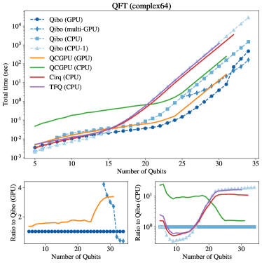
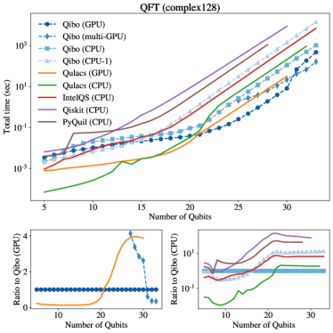
Figure 2: Quantum Fourier Transform simulation performance comparison in single precision (left) and double precision (right). Large plots show total simulation time as a function of qubit number. Smaller plots show the ratio of this time for each library to the corresponding Qibo run for GPU (left) and CPU (right).

The first circuit we used for benchmarks is the Quantum Fourier Transform (QFT) [8]. This circuit is used as a subroutine in many quantum algorithms and thus constitutes an example with great practical importance. The gates used in this circuit are H, CZPow, and SWAP, all of which are available in Qibo and other used libraries, except QCGPU where SWAP was implemented using three CNOT gates.

Results for the QFT circuit are shown in Fig. 2. It is natural to discuss two regimes separately, the small circuit regime consisting of up to 20 qubits and the large circuit regime for more than 20 qubits. We observe that most libraries offer similar performance in the first regime. Qulacs is the fastest as it is based on compiled C++ and avoids the Python overhead that exists in all other libraries. Furthermore, we observe that simpler hardware configurations (single-thread CPU) perform better for small circuits than more complex ones (multi-threading or GPU). In the large circuit regime Qibo offers a better scaling than other libraries in both CPU and GPU. It is also clear that GPU accelerated libraries offer about an order of magnitude improvement compared to CPU implementations. We note the exact agreement between TFQ and single-thread Qibo as both libraries use TensorFlow as their computation engine.

In terms of memory, Qibo can simulate the highest number of qubits (33 in complex128 / 34 in complex64) possible for the memory available in the DGX station (256 GB). A single 32 GB GPU can simulate up to 30 qubits (31 in complex64), however this number can be extended up to 33 (34 in single precision) using the distributed scheme described in Sec. 2.5 to re-use the same GPU device on multiple state vector partitions. The switch from single to distributed GPU configuration explains the change of scaling in the last three points of “Qibo (GPU)” data. The distributed scheme can achieve an even better scaling if all four available DGX GPUs are used (“Qibo (multi-GPU)” line). For more details on the performance of different hardware configurations supported by Qibo, we refer to Sec. 3.6.

Figure 3: Structure of the variational circuit used in the benchmarks. All gates shown in this figure are repeated five times to give the full circuit and an additional layer of RY gates is used in the end.

3.2 Variational circuit

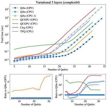
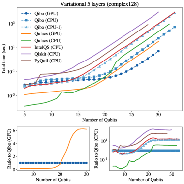
Figure 4: Variational circuit simulation performance comparison in single precision (left) and double precision (right). Large plots show total simulation time as a function of number of qubits. Smaller plots show the ratio of this time for each library to the corresponding Qibo run for GPU (left) and CPU (right).

The second circuit used in the benchmarks is inspired by the structure of variational circuits used in quantum machine learning and similar applications  [13, 14]. Such circuits constitute a good candidate for applications of near-term quantum computers due to their short depth and are of great interest to the research community. The circuit used in the benchmark consists of a layer of RY rotations followed by a layer of CZ gates that entangle neighbouring qubits, as shown in Fig. 3. The configuration is repeated for five layers and the variational parameters are chosen randomly from $[0,2\pi]$ in all benchmarks.

In Fig. 4 we plot the results of the variational circuit benchmark. We observe similar behavior to the QFT benchmarks with all libraries performing similarly for small qubit numbers and Qibo offering superior scaling for large qubit numbers. The variational circuit is an example where the gate fusion described in Sec. 2.4 is useful. In our Qibo implementation we exploit this by using the Variational-
Layer gate, which fuses four RY gates with the CZ gate between them and applies them as a single two-qubit gate. TFQ uses a similar fusion algorithm [20], and unlike the QFT benchmark, it is now noticeably faster than Cirq. All other libraries use the traditional form of the circuit, with each gate being applied separately.

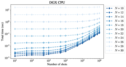
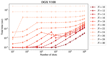
Figure 5: Example of measurement shots simulation on CPU (left) and GPU (right).

3.3 Measurement simulation

Qibo simulates quantum measurements using its standard dense state vector simulator, followed by sampling from the distribution corresponding to the final state vector. Since the dense state vector is used instead of repeated circuit executions, measurement time does not have a strong dependence on the number of shots. This is demonstrated for different qubit numbers $N$ in Fig. 5. The plots contain only the time required for sampling as the state vector simulation time (time required to apply gates) has been subtracted from the total execution time. The circuit used in this benchmark consists of a layer of H gates applied to every qubit followed by a measurement of all qubits.

When a GPU is used for a circuit that contains measurements, it will likely run out of memory during the sampling procedure if the number of shots is sufficiently high. In such a case, Qibo will automatically fall back to CPU to complete the execution. This is not particularly costly in terms of performance as the computationally heavy part is the evolution of the state vector, which happens on GPU, and not the sampling procedure. The oscillations that appear in the GPU part of Fig. 5 are due to this fallback mechanism. This is implemented using an exception on TensorFlow’s out-of-memory error, and as a result, the procedure of falling back to CPU is slower than explicitly executing sampling on CPU.

3.4 Simulation precision

Qibo allows the user to easily switch between single (complex64) and double (complex128) precision with the qibo.set_precision() method. In this section we compare the performance of both precisions. The results are plotted in Fig. 6. We find that as the number of qubits grows using single precision is $\sim 2$ times faster on GPU and $\sim 1.5$ faster on CPU.

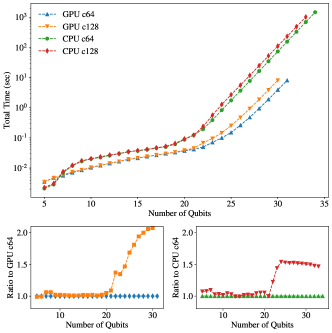
Figure 6: Comparison of simulation time when using single (complex64) and double (complex128) precision on GPU and multi-threading (40 threads) CPU.

3.5 Adiabatic time evolution

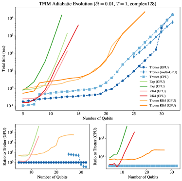
Figure 7: Adiabatic time evolution simulation performance comparison in double precision. Large plots show total simulation time as a function of qubit number. Smaller plots show the ratio of this time to the corresponding Trotter evolution run for GPU (left) and CPU (right).

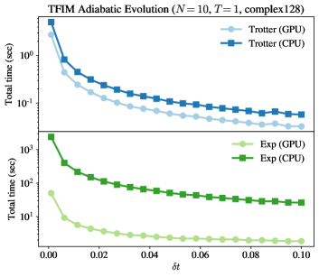
Figure 8: Total execution time for the adiabatic evolution of $N=10$ for total time $T=1$ as a function of the time step $\delta t$.

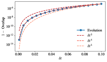
Figure 9: Overlap between the final state obtained using the Trotter decomposition and the full exponentiation of the Hamiltonian. The problem considered is the adiabatic evolution of the TFIM Hamiltonian (Eq. (5)) for total time $T=1$, linear scheduling and $N=10$ qubits.

We use Qibo to simulate the adiabatic evolution with the Hamiltonians defined in Eq. (5) and linear scaling $s(t)=t$. We simulate for a total time of $T=1$ using double precision.

The total simulation time is shown as a function of the number of qubits in Fig. 7 for execution on CPU (40 threads) and GPU. As expected, using the Trotter decomposition is several orders of magnitude faster than methods that use the full $2^{N}\times 2^{N}$ Hamiltonian matrix. It also requires less memory allowing the simulation of larger qubit numbers. Note that using Runge-Kutta methods with a Trotter Hamiltonian requires less memory because it calculates the dot products between the Hamiltonian and the state term by term, instead of constructing the full matrix.

Similar to circuit simulation, GPU is typically faster than CPU for all solvers. Note that similarly to the QFT benchmarks shown in Fig. 2 the last few points of the “Trotter (GPU)” line correspond to re-using the same device using the distributed scheme leading to a different scaling in the execution time. Runge-Kutta solvers exploit parallelization techniques less than other methods and, as a result, have the smallest speed-up from using a GPU. In all cases, the time direction has to be treated sequentially, while the matrix multiplications at a given time step can be computed in parallel, making the GPU more useful as the number of qubits increases.

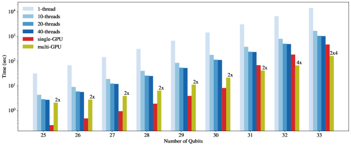
Figure 10: Comparison of Qibo performance for QFT on multiple hardware configurations. For the multi-GPU setup we include a label on top of each histogram bar summarizing the effective number of NVIDIA V100 cards used during the benchmark.

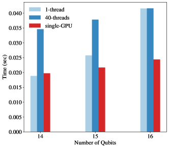
Figure 11: Comparison of Qibo performance for small QFT circuits on single thread CPU, multi-threading CPU and GPU. Single thread CPU is the optimal choice for up to 15 qubits.

In Fig. 8 we plot the total execution time as a function of the time step $\delta t$ used to discretize time. The exponential solver is used with and without Trotter decomposition. In Fig. 9 we calculate the underlying errors of the Trotter decomposition. The error is quantified using the overlap between the final state obtained using the Trotter decomposition and the full exponential time evolution operator, with the latter considered to be exact. We find that as we decrease the time step $\delta t$ the overlap approaches unity as $\delta t^{4}$, but execution time increases as expected. The $\delta t^{n}$ lines for $n\in\{3,4,5\}$ in Fig. 9 correspond to curves defined by $y=y_{0}\left(\frac{x}{x_{0}}\right)^{n}$ where $(x_{0},y_{0})$ is the rightmost point (for $\delta t=0.1$) in the “Evolution” curve. These are plotted to demonstrate the scaling of evolution error as $\delta t\rightarrow 0$.

3.6 Hardware device selection

Number of qubits	0-15	15-30	$>30$
CPU single thread	$\star\star\star$	$\star$	$\star$
CPU multi-threading	$\star$	$\star\star$	$\star\star$
single GPU	$\star$	$\star\star\star$	$\star\star$
multi-GPU	-	-	$\star\star\star$

Table 5: Heuristic rules for optimal device selection depending on the number of qubits in the circuit. More stars means a shorter execution time is expected. We stress that these general rules may not be valid on every case as the optimal configuration depends on many factors such as the exact circuit structure and hardware specifications (CPU and GPU speed and memory).

A core point in Qibo is the support of different hardware configurations despite its simple installation procedure. The user can easily switch between CPU and GPU using the qibo.set_device() method. A question that arises is how to determine the optimal device configuration for the circuit one would like to simulate. While the answer to this question depends both on the circuit specifics (number of qubits, number of gates, number of re-executions) and the exact hardware specifications (CPU or GPU model and available memory), in this section we provide a basic comparison using the DGX station. The circuit used is the QFT in double precision, and the results of this section are summarized in Table 5, which provides some heuristic rules for optimal device selection according to the number of qubits.

In Fig. 10 we plot the total simulation time using four different CPU thread configurations and two GPU configurations. The number of threads in the CPU runs was selected using taskset. For large numbers of qubits we observe that using multiple threads reduces simulation time by an order of magnitude compared to single-thread. However, performance plateaus are reached at 20-threads. Switching to a GPU whenever the full state vector fits in its memory provides an additional 10x speed-up making it the optimal device choice for circuits containing 15 to 30 qubits.

The situation is less clear for circuits with more than 30 qubits, when the full state vector does not fit in a single GPU memory. Qibo provides three alternative solutions for such situation: multi-threading CPU, re-using a single GPU for multiple state pieces (mimicking distributed computation) or using multiple GPUs if available. In terms of memory, all these approaches are limited by the total memory available for the system’s CPU. Using multiple GPUs is always more efficient than re-using a single GPU as it allows us to parallelize the calculations on different state pieces.

The comparison between multi-GPU and CPU generally depends on the structure of the circuit. QFT is an example of a circuit that does not require any additional SWAP gates between global and local qubits, making it a good case for a distributed run. This property is not true for all circuits, and therefore we would see a smaller difference between CPU and multi-GPU configurations for other circuits. Regardless, multi-GPU configurations or even re-using a single GPU are expected to be useful for the regime of qubit numbers between 30 and 35.

In Fig. 11 we repeat the hardware comparison for smaller qubit numbers. We find that single thread CPU is the optimal choice for up to 15 qubits, while the GPU will start giving an advantage beyond this point.

4 Applications

The current Qibo 0.1.0 contains pre-coded examples of quantum algorithms applied to specific problems. The subsections that follow provide an outline of these applications. For more details on each application we refer to our documentation [72] and we note that all the code is available at the Qibo repository.

It is worth emphasizing that, apart from the application examples that follow, Qibo provides several application-specific models, in addition to the standard models.Cir-
cuit that can be used for circuit simulation. These models are outlined in Table 2 and some are used in the applications that follow.

4.1 Variational Quantum Eigensolver

The Variational Quantum Eigensolver (VQE) [60] is a common technique for finding ground states of Hamiltonians in the context of quantum computation. As noted in Table 2, Qibo provides a VQE model that allows optimization of the variational parameters.

In this example, we provide an extension of the VQE algorithm that may be used to improve optimization and is known as the adiabatically assisted VQE (AAVQE) [73]. Qibo provides a pre-coded implementation of the AAVQE for finding the ground state of the transverse field Ising Hamiltonian defined in Eq. (5) and can be executed for any number of qubits, variational circuit layers and number of adiabatic steps specified by the user. Particularly, the example may be used to explore how the accuracy of the VQE ansatz scales with the underlying circuit depth, as presented in [74].

The code below demonstrates how the AAVQE can be implemented in Qibo.

⬇

# loop over the adiabatic steps

for t in range(T_max + 1):

# define the interpolated Hamiltonian of AAVQE

s = t / T_max

hamiltonian = (1-s) * h0 + s * h1

# define a Qibo VQE model

vqe = models.VQE(circuit, hamiltonian)

# optimize the VQE model to find that ground state

options = {’maxfev’: maxsteps}

energy, params = vqe.minimize(initial_params,

method=’Nelder-Mead’,

options=options)

initial_params = params

where h0 and h1 are hamiltonians.Hamiltonian objects representing the easy and hard Hamiltonian respectively, circuit is a models.Circuit that implements the VQE ansatz, initial_params (np.ndarray) is the initial guess for the variational parameters, T_max (int) the number of adiabatic steps and maxsteps (int) the maximum number of optimization steps.

4.2 Grover’s search for 3SAT

Grover’s algorithm [10] is a quantum algorithm for searching databases and an example where a quantum computer provides a quadratic advantage $\sqrt{2^{N}}$, where $N$ is the number of qubits, over a classical one for the same problem. In this example, Grover’s algorithm is used to solve exact cover instances of a 3SAT problem, which is classified as NP-Complete [75].

In terms of implementation, Grover’s algorithm can be simulated by defining a Qibo circuit that contains the required gates, which implement the oracle and the diffusion transformation. The pre-coded example comes with several instances of the exact cover problem from 4 up to 30 bits, where the solution is known, so that the user can verify that the algorithm has been successful, and that the solution is indeed the measured bitstring. Moreover, the user may execute the algorithm to newly created instances, with a known or unknown solution.

4.3 Grover’s search for hash functions

A second application of Grover’s algorithm [10] implemented in Qibo is on the task of finding the preimages of a hash function based on the ChaCha permutation [76]. The example is based on Ref. [77].

In this case, the example takes as input a hash integer of 8 or fewer bits and finds the corresponding preimage, that is the number that maps to the given hash when applying the permutation. If the number of collisions is known for the given hash then the algorithm finds all the possible solutions. Here collisions refers to the number of solutions. If the number of collisions is not given then the algorithm finds one solution using an iterative procedure [78].

4.4 Quantum classifier

This example provides a variational quantum algorithm for classifying classical data [79]. The optimal values for the variational parameters are found via supervised training, minimizing a local loss given by the quadratic deviation of the classifier’s predictions from the actual labels of the examples in the training set.

The pre-coded Qibo example applies the classifier on the iris data set [80]. The user has the option to train the circuit from scratch or use several pre-trained configurations to make predictions and calculate the classification accuracy. The user can also select the number of qubits and the circuit depth.

4.5 Quantum classifier using data reuploading

Similarly to the previous section, this example provides a variational algorithm for classifying classical data using only one qubit and is based on Ref. [81]. The main idea is reuploading, that is creating a single qubit circuit where several different unitary gates are applied and each gate depends on the point that is classified and a set of variational parameters that are optimized through a learning procedure.

The pre-coded Qibo example applies such classifier on various two-dimensional classical datasets. The user can choose between training the classifier from scratch (optimizing the variational parameters) or using the provided pre-trained models. The code can be used to measure the accuracy of the classifier in each classification task and also provides plots with labeled points, using different colors for each class. Plots are provided in the two-dimensional plane but also on the Bloch sphere.

4.6 Quantum autoencoder for data compression

The task of an autoencoder is to map an input density matrix $\mathbf{x}$ to a lower-dimensional Hilbert space $\mathbf{y}$, such that $\mathbf{x}$ can be recovered from $\mathbf{y}$. The quantum autoencoder that is implemented in Qibo is based on [82] and is used to encode the ground states of the transverse field Ising model (Eq. (5)) for various $h$-field values.

The code below demonstrates how the autoencoder optimization can be simulated using Qibo

⬇

def cost(params):

”””Calculates loss for specific values of parameters.”””

circuit.set_parameters(params)

for state in ising_groundstates:

final_state = circuit(np.copy(state))

cost += encoder.expectation(final_state).numpy().real

\paroptions = {’maxiter’: 2.0e3, ’maxfun’: 2.0e3}

result = minimize(cost, initial_params,

method=’L-BFGS-B’,

options=options)

where circuit is a Qibo circuit that implements the variational ansatz, ising_groundstates is a list of the states to be encoded and encoder is a Hamiltonian object for $-\sum_{i=1}^{N}Z_{i}$ properly rescaled.

4.7 Quantum singular value decomposer

The quantum singular value decomposer (QSVD) [83] refers to a circuit that produces the Schmidt coefficients of a pure bipartite quantum state. This is implemented as follows: Two Qibo variational circuits are defined and measured, one acting on each part of the bipartite measurements. The variational parameters are tuned to minimize a loss that depends on the Hamming distance of the two measured bitstrings. The user may attempt this optimization using the pre-coded example for random initial bipartite states with an arbitrary number of qubits and partition sizes.

4.8 Tangle of three-qubit states

This example provides a variational strategy to compute the tangle of an unknown three-qubit state, given many copies of it. It is based on the result that local unitary operations cannot affect the entanglement of any quantum state and follows Refs. [84, 85]. An unknown three-qubit state is received, and one unitary gate is applied on every qubit. The exact gates are obtained such that they minimize the number of outcomes of the states $|001\rangle$, $|010\rangle$ and $|011\rangle$. The code can be used to simulate both noiseless and noisy circuits.

4.9 Unary approach to option pricing

This is an example application of quantum computing in finance and provides a new strategy to compute the expected payoff of a (European) option, based on Ref. [86]. The main feature of this procedure is to use the unary encoding of prices, that is, to work in the subspace of the Hilbert space spanned by computational-basis states where only one qubit is in the $|1\rangle$ state. This allows for a simplification of the circuit and resilience against errors, making the algorithm more suitable for NISQ devices.

The pre-coded example takes as input the asset parameters (initial price, strike price, volatility, interest rate and maturity date) and the quantum simulation parameters (number of qubits, number of measurement shots and number of applications of the amplitude estimation algorithm (see [86])) and calculates the expected payoff using the quantum algorithm. The result is compared with the exact value of the expected payoff. Furthermore, the code plots a histogram of the quantum estimation for the option price probability distribution and a plot of the amplitude estimation measurement results as a function of iterations.

4.10 Adiabatic evolution

As noted in Table 2, Qibo provides models for simulating the unitary time evolution of quantum states, with a specific application on adiabatic evolution. As examples, we provide scripts that apply these models in various physics applications.

The first example simulates the adiabatic evolution of an Ising Hamiltonian (Eq. (5)) for $h=1$ using a linear scaling function $s(t)=t/T$, where $T$ is the total evolution time. Executing this example shows plots with the dynamics of energy (expectation value of the Ising Hamiltonian) and the overlap between the evolved state and the exact Ising ground state. Using these plots, we verify that the evolution converges to the exact ground state if sufficient evolution time $T$ is used.

In addition, we provide the possibility to optimize the scheduling function $s(t)$ and final time $T$ so that the actual ground state is reached in a shorter time. The free parameters of $s(t)$ and $T$ are optimized so that the energy of the final state of the evolution is minimized. In our example, we use a polynomial ansatz for $s(t)$ where the coefficients are the free parameters that are optimized.

4.11 Adiabatic evolution for 3SAT

Adiabatic evolution can also be applied to optimization problems outside physics. In this example, we provide an application for solving exact cover instances of a 3SAT problem, which is classified as an NP-Complete problem [75]. The same problem was solved in Sec. 4.2 using Grover’s algorithm in the circuit based paradigm of quantum computation, while in this example we demonstrate that a quantum annealing approach is also possible [87].

Similarly to Sec. 4.2, the user may use one of the provided instances of the exact cover problem or add a custom one. The pre-coded example accepts the instance and the evolution parameters (total time $T$, discretization time step $\delta t$, and method of integration) and computes the solution and the probability that this is measured. The Trotter decomposition may be used for a more efficient evolution simulation. Additionally, for sufficiently small systems (due to memory constraints), it is possible to calculate and plot the gap of the adiabatic Hamiltonian as a function of time.

This example uses a linear scaling function by default. It is possible to switch to a polynomial scaling function and also optimize the underlying coefficient so that the solution is found in smaller total time $T$. Performing such optimization, we find that a scaling function that is “slower” at times where the gap is small is preferred over the default linear scheduling.

5 Outlook

Qibo provides a new interface for quantum simulation research by granting users and researchers the ability to implement quantum algorithms with simplicity. The user is allowed to simulate circuits and adiabatic evolution on different hardware platforms without having to know about the technicalities or the difficulties of their implementation on data placement, multi-threading systems and memory management that GPU and multi-GPUs computing require.

In this first release, Qibo includes a high-performance framework for quantum circuit simulations and adiabatic evolution using linear algebra techniques in combination with hardware acceleration strategies. For the time being, the code is targeted to run on single node devices with single or multiple GPU cards and sufficient RAM in order to perform simulations with an acceptable number of qubits and computational time.

The roadmap for future releases is organized in two directions. The first direction is focused on Physics and new algorithms for specific applications, in order to extend the code base set of algorithms for quantum calculations. Some imminent examples are the implementation of noise density matrices for custom operators and noise simulation without density matrices. The second direction is based on the technical perspective. We plan to extend the current distributed computation model to support multi-node devices through the OpenMPI [88, 89] interface.

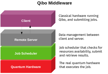
Figure 12: Schematic view of the Qibo middleware design.

Furthermore, in Fig. 12 we show schematically how the Qibo framework will be integrated with the middleware of the new quantum hardware developed by [57, 58]. The middleware infrastructure will provide the possibility to submit quantum calculations, defined with the Qibo API, to the quantum hardware through a server scheduling and queue service that provide the possibility to submit and retrieve results from the quantum computer laboratory. This development is particularly important in order to achieve the evaluation of quantum circuits, adiabatic evolution, and hybrid computations on the real quantum hardware.

References

-
[1]
Google Research,
Google AI
Quantum (2017).
URL https://research.google/teams/applied-science/quantum/ -
[2]
IBM Research, IBM Quantum
Experience (2016).
URL https://www.ibm.com/quantum-computing/ -
[3]
Rigetti, Rigetti Computing (2017).
URL https://www.rigetti.com/ -
[4]
Intel Corporation,
Intel
Quantum Computing (2017).
URL https://www.intel.com/content/www/us/en/research/quantum-computing.html -
[5]
D-Wave Systems, The Quantum Computing
Company (2011).
URL https://www.dwavesys.com/ -
[6]
D-Wave Systems, D-Wave
Neal.
URL https://github.com/dwavesystems/dwave-neal - [7] F. Arute, et al., Quantum supremacy using a programmable superconducting processor, Nature 574 (2019) pp. 505–510. doi:10.1038/s41586-019-1666-5.
- [8] D. Coppersmith, An approximate fourier transform useful in quantum factoring (2002). arXiv:quant-ph/0201067.
- [9] G. Brassard, P. Hoyer, M. Mosca, A. Tapp, Quantum amplitude amplification and estimation (2000). arXiv:quant-ph/0005055.
- [10] L. K. Grover, A fast quantum mechanical algorithm for database search (1996). arXiv:quant-ph/9605043.
- [11] L. K. Grover, Quantum computers can search rapidly by using almost any transformation, Physical Review Letters 80 (19) (1998) 4329–4332. doi:10.1103/physrevlett.80.4329.
- [12] M. A. Nielsen, I. L. Chuang, Quantum computation and quantum information (2010). doi:10.1017/CBO9780511976667.
- [13] N. Moll, et al., Quantum optimization using variational algorithms on near-term quantum devices, Quantum Science and Technology 3 (3) (2018) pp. 030503. doi:10.1088/2058-9565/aab822.
- [14] E. Farhi, J. Goldstone, S. Gutmann, A quantum approximate optimization algorithm (2014). arXiv:1411.4028.
- [15] P. W. Shor, Polynomial-time algorithms for prime factorization and discrete logarithms on a quantum computer, SIAM Review 41 (2) (1999) pp. 303–332. doi:10.1137/S0036144598347011.
- [16] S. Boixo, S. V. Isakov, V. N. Smelyanskiy, H. Neven, Simulation of low-depth quantum circuits as complex undirected graphical models (2017). arXiv:1712.05384.
- [17] J. Chen, et al., Classical simulation of intermediate-size quantum circuits (2018). arXiv:1805.01450.
- [18] I. L. Markov, Y. Shi, Simulating quantum computation by contracting tensor networks, SIAM Journal on Computing 38 (3) (2008) pp. 963–981. doi:10.1137/050644756.
-
[19]
Cirq, a python framework for
creating, editing, and invoking Noisy Intermediate Scale Quantum (NISQ)