Dynamics of magnetic collective modes in the square and triangular lattice
Mott insulators at finite temperature

Abstract

We study the equilibrium dynamics of magnetic moments in the Mott insulating phase of the Hubbard model on the square and triangular lattice. We rewrite the Hubbard interaction in terms of an auxiliary vector field and use a recently developed Langevin scheme to study its dynamics. A thermal noise, derivable approximately from the Keldysh formalism, allows us to study the effect of finite temperature. At strong coupling, $U\gg t$, where $U$ is the local repulsion and $t$ the nearest neighbour hopping, our results reproduce the well known dynamics of the nearest neighbour Heisenberg model with exchange $J\sim{\cal O}(t^{2}/U)$. These include crossover from weakly damped dispersive modes at temperature $T\ll J$ to strong damping at $T\sim{\cal O}(J)$, and diffusive dynamics at $T\gg J$. The crossover temperatures are naturally proportional to $J$. To highlight the progressive deviation from Heisenberg physics as $U/t$ reduces we compute an effective exchange scale $J_{eff}(U)$ from the low temperature spin wave velocity. We discover two features in the dynamical behaviour with decreasing $U/t$: (i) the low temperature dispersion deviates from the Heisenberg result, as expected, due to longer range and multispin interactions, and (ii) the crossovers between weak damping, strong damping, and diffusion take place at noticeably lower values of $T/J_{eff}$. We relate this to enhanced mode coupling, in particular to thermal amplitude fluctuations, at weaker $U/t$. A comparison of the square and triangular lattice reveals the additional effect of geometric frustration on damping.

I Introduction

The Hubbard model at half-filling provides a minimal description of an interaction driven Mott metal-insulator transition zhang ; imada ; rozenberg ; capone ; park ; ohashi1 ; ohashi2 ; furukawa ; sahebsara ; yamada1 (MIT). The Mott phase generally has some kind of antiferromagnetic order sahebsara ; yamada1 , except in fully frustrated lattices like the Kagome or pyrochlore where it has only short range correlations bulut ; ohashi1 ; furukawa ; yamada2 ; kita ; fujimoto ; normand ; swain . The static charge and magnetic correlations are reasonably well understood in the various lattices hirsch ; white ; hrk ; zimmermann ; fazekas ; tasaki ; hochkeppel ; watanabe ; yoshioka ; tocchio1 ; tocchio2 ; kokalj ; goto ; shirakawa ; li .

Theoretical results on dynamics are more limited. Approaches like dynamical mean field theory (DMFT) or its extensions, which provide a detailed description of the MIT, focus on the single particle spectral function DMFT ; bulla ; zitko ; eckstein ; peters ; kitatani . The collective mode dynamics associated with the magnetic degrees of freedom is much less explored kotliar1 ; schulz ; ho ; singh1 ; singh2 ; singh3 ; gunnarsson ; chern ; leblanc1 , although in the Mott phase, where single particle excitations are gapped, these are in fact the relevant degrees of freedom.

Deep in the insulating phase, where the Hubbard model maps on to the nearest-neighbour Heisenberg model fazekas ; cleveland , the spin dynamics is well documented blume1 ; blume2 ; takahashi ; gouvea ; volkel ; peczak ; costa ; moessner ; taillefumier ; sherman . However, on decreasing the electron-electron interaction two effects occur simultaneously: (i) the coupling among magnetic moments become progressively longer ranged, multi-spin, and begin to involve ring-exchange terms capriotti ; yang , and (ii) the moments begin to “soften”, i.e, become more prone to amplitude fluctuations. The first effect affects mainly the low temperature spin-wave dispersion. The second effect is important for the thermal physics since amplitude fluctuations generate additional scattering of the magnetic modes. In a Mott insulator where the charge gap is $\sim 10^{3}-10^{4}$K, say, and the effective exchange is $\sim 10-100$K these effects would be visible over an accessible temperature window.

Experiments on dynamics in Mott insulating materials have mostly concentrated on quasi-2d systems like layered cuprates aeppli ; coldea ; stock , organics kurosaki ; powell , ruthenates friedt ; steffens and fully 3d systems like iridates shapiro ; choi ; tomiyasu ; bahr , doped V₂O₃ bao , NiO kim and Sr₂Mn₃As₂O₂ chen . In the Mott phase, inelastic neutron scattering (INS) studies on La₂CuO₄ find substantial non-Heisenberg features in the dispersion. In the iridate experiments, one infers no long-range magnetic order shapiro in some cases, while in certain others choi ; tomiyasu ; bahr , sharp low-energy spin waves originating from complex magnetic order are observed. Near the transition, NMR measurements on organics have found strong suppression of spin fluctuations in the Mott phase. By contrast, in Ca_2-xSr_xRuO₄, one finds enhanced magnetic fluctuations in the metallic phase at an incommensurate wave vector.

A reliable estimate of the magnetic excitation spectrum requires several ingredients: (i) one should be able to handle correlation effects away from the Heisenberg limit, in particular as the system heads towards an insulator-metal transition, (ii) the dimensionality and lattice geometry needs to be respected since the magnetic order and excitations depend crucially on them, (iii) the approach should access thermal effects well beyond the reach of linear spin wave theory, and (iv) the theory should yield real time (or real frequency) information - a rarity in finite temperature schemes. Most approaches unfortunately fall short.

The tools currently available to study equilibrium dynamics of the Hubbard model include exact methods like quantum Monte Carlo QMC (QMC), approximate numerical strategies like DMFT DMFT ; kotliar2 and its cluster extensions park ; hochkeppel , slave boson techniques fresard , and semi-analytic schemes like the random phase approximation (RPA) or $1/S$ expansion. More recently, dual fermion method leblanc1 ; li , and semiclassical Langevin dynamics chern have entered the scenario. A recent review covers most of the existing approaches used for the 2d model leblanc2 . Both QMC and DMFT are usually formulated in imaginary time, and hence the results need analytic continuation. QMC also has size limitations and often the ”fermion sign problem”. DMFT neglects spatial correlations at the single site level, but its cluster variants alleviate the problem in some cases. The RPA approach yields reasonable low-temperature spin wave dispersion ($\Omega_{\bf q}$) on magnetically ordered states singh1 ; singh2 ; singh3 and also captures high-energy features like the two-particle continuum. However, as order is suppressed with increasing temperature, and large angular fluctuations become relevant, the RPA results lose validity.

An approximate strategy well suited for this problem is the Langevin dynamics approach, first introduced by Chern et. al. chern . This method does make some simplifying assumptions but meets all the requirements that we had defined earlier. Using this we address the following questions: (i) how are the crossover scales in magnetic dynamics affected as we move to lower values of $U/t$ from the Heisenberg limit? (ii) what is the role of amplitude fluctuations on the lineshape of excitations, and (iii) what is the effect of increasing geometric frustration on the spectrum?

There are two ”reference calculations” that define what is known in this problem. (a) For $U/t\gg 1$ and for nearest neighbour hopping the Hubbard model maps on to the nearest neighbour Heisenberg model. The ground state on the square lattice is Néel ordered with ${\bf Q}=(\pi,\pi)$, while on the triangular lattice ${\bf Q}=(2\pi/3,2\pi/3)$. The relevant exchange scale is $J=4t^{2}/U$, for moments with $S=1/2$. The thermal dynamics of the Heisenberg model is well known blume1 ; blume2 ; takahashi ; gouvea ; volkel ; peczak ; costa ; moessner ; taillefumier ; sherman , albeit numerically. (b) On the mean field ground state, RPA provides a reasonable excitation spectrum at any $U/t$.

We have confirmed that the Langevin scheme captures the dynamics of the 2d classical Heisenberg model on both lattices, at all temperature. Since we approximate the magnetic moments in our scheme to be classical, we do not get the true quantum limit at large $U/t$. Our theory also captures the low energy part of the RPA spectrum at all $U/t$ and low temperature, but not the spin waves at zero temperature.

To set the stage for a summary of our results, the magnetic dynamics can be classified into three regimes. (A). At low temperature we observe weakly damped dispersive modes, with damping $\Gamma_{\bf q}\ll W_{mag}$, where $W_{mag}$ is the magnetic bandwidth at $T=0$. This scale is plotted in Fig.2(b). In this regime in general $\Gamma_{\bf q}\ll\Omega_{\bf q}$. (B). Beyond a broad crossover, characterised by a scale $T^{cr}_{1}$, there is a regime of strongly damped but still dispersive modes, with $\Gamma_{\bf q}\sim{\cal O}(W_{mag})$. Finally, (C). at even higher temperature, beyond a scale $T_{2}^{cr}$, we observe spin diffusion, with $\Omega_{\bf q}\rightarrow 0$ for all ${\bf q}$ and $\Gamma_{\bf q}\sim{\cal O}(W_{mag})$.

An important scale in analyzing the results is the effective exchange $J_{eff}(U)$, inferred from the spin wave velocity computed from the low energy spectrum. The spin wave velocity is the slope of the linear magnon branch near the Goldstone points, $(\pi,\pi)$ and $(2\pi/3,2\pi/3)$ for the square and triangular lattice, respectively. $J_{eff}$ is plotted in Fig.2(a). In terms of this scale, our main results are the following - first on the square lattice, and then on the triangular lattice.

I. For the square lattice:

• Broad regimes: While the absolute values of the crossover temperatures increase with decreasing $U/t$ (since the effective exchange $J_{eff}$ increases), the ratios $T^{cr}_{1}/J_{eff}$ and $T^{cr}_{2}/J_{eff}$ noticeably decrease with decreasing $U/t$. This indicator of non-Heisenberg behaviour suggests a relatively quicker onset of mode coupling, and then diffusive behaviour, at smaller $U/t$.

• Dispersion and damping: The dispersion $\Omega_{\bf q}(T)$ narrows monotonically with increasing $T/J_{eff}$, The onset of rapid narrowing is at $T/J_{eff}\sim 1$ when $U/t\gg 1$ and reduces to $T/J_{eff}\sim 0.5$ for $U\sim 6t$. We find that at low $T$ the thermal damping is $\Gamma_{\bf q}(T)-\Gamma_{\bf q}(0)\propto T^{2}$ when $U/t\gg 1$ and $\Gamma_{\bf q}(T)-\Gamma_{\bf q}(0)\propto T$ for intermediate to small $U/t$. The damping changes to $\sim T^{1.5}$ at higher $T$, and finally saturates for $T\gtrsim 2J_{eff}$.

• Amplitude fluctuation: The amplitude fluctuations play a crucial role in broadening the lineshape at weak coupling, where the fluctuation width varies as $\sim\sqrt{T/U}$. While we do not capture the real ”amplitude mode” at $\omega\sim U$ we can access amplitude fluctuation effects on the spin waves at $\omega\sim J_{eff}$.

II. On the triangular lattice:

• Broad regimes: The triangular lattice has a finite critical interaction for the MIT, with $U_{c}\sim 5t$. We restrict ourselves to $U/t$ where the 120°ordered state is the ground state. The typical lineshape is two-peak in this case. The thermal crossover scales are inferred from the behaviour of the peak which broadens quicker with respect to $T$. The behaviour of $T^{cr}_{1}$ and $T^{cr}_{2}$ with respect to $U$ is similar to what is observed in the square lattice, with the distinction that their maxima occur at larger $U$ and the scales are $\sim 0.5$ their square lattice values.

• Dispersion and damping: Due to emergence of longer range couplings, the low $T$ dispersion along $\Gamma-K$ shows a larger curvature at lower $U/t$. The damping is also much larger, compared to the square lattice, at similar values of $T/J_{eff}$. At $U/t\sim 10$, where $J_{eff}/t\sim 0.04$ the crossover scales are just $T^{cr}_{1}/J_{eff}\sim 0.4$ and $T^{cr}_{2}/J_{eff}\sim 0.8$.

• Fluctuation: The role of amplitude fluctuations in damping the modes is enhanced at a given $U$ and the same $T/J_{eff}$, due to the finite $U_{c}$ and mild frustration.

II Model and method

We work with the single band, repulsive Hubbard model on square and triangular lattice geometries. The Hamiltonian reads-

$$H=-\sum_{<ij>\sigma}t_{ij}(c^{\dagger}_{i\sigma}c_{j\sigma}+h.c.)+U\sum_{i}n_{i\uparrow}n_{i\downarrow}-\mu\sum_{i\sigma}n_{i\sigma}$$

The hopping amplitude $t_{ij}$ is chosen to be non-zero only amongst nearest neighbours for the square case and has a uniform value $t=1.0$. On adding the next-nearest neighbour coupling $t^{\prime}=1.0$ on top of this along one diagonal in each square motif, we get the triangular lattice.

First, the interaction term is decoupled using a Hubbard-Stratonovich transformation to obtain a spin-fermion model-

$$H_{SF}=-\sum_{<ij>\sigma}t_{ij}(c^{\dagger}_{i\sigma}c_{j\sigma}+h.c.)-U\sum_{i}{\bf m}_{i}.\sigma_{i}+U\sum_{i}|{\bf m}_{i}|^{2}$$

We solve for the finite $T$ dynamics ${\bf m}_{i}$ using the following equation of motion chern :

$$\frac{d{\bf m}_{i}}{dt}=-{\bf m}_{i}\times\frac{\partial\langle H_{SF}\rangle}{\partial{\bf m}_{i}}-\gamma\frac{\partial\langle H_{SF}\rangle}{\partial{\bf m}_{i}}+\vec{\xi}_{i}$$ (1)

The noise is specified through-

$$\langle\xi^{\mu}_{i}(t)\rangle = 0$$ (2)

$$\langle\xi^{\mu}_{i}(t)\xi^{\nu}_{j}(t^{\prime})\rangle = 2\gamma k_{B}T\delta_{ij}\delta^{\mu\nu}\delta(t-t^{\prime})$$ (3)

Here $\gamma$ is a dissipation parameter. Within our scheme, it’s value can’t be determined from first principles. To calculate it, one has to evaluate the imaginary part of the Keldysh polarizability ($Im\Pi^{K}({\bf q},\omega)$) at low frequencies. We comment that in the deep Mott phase, this contribution is vanishingly small due to the gapped single electron spectrum. However, on moving to lower $U$ values, this quantity picks up weight at finite temperature. The evolution equation has a phenomenological justification as well as a a microscopic basis. We touch on these briefly.

I. First the phenomenological motivation chern ; ma . One starts from the Heisenberg limit with moments of fixed magnitude. The torque term comes from evaluating the Poisson brackets in the semiclassical equation of motion. The damping is taken to be proportional to the angular momentum, following an analogy with the particle Langevin equation. Lastly, the noise is chosen so as to satisfy the fluctuation-dissipation relation, ensuring that one captures the Boltzmann distribution in the long-time limit ma ; kirilyuk . The additive form of the damping and noise allows for longitudinal relaxation of the magnetic moments. This approach does not determine the value of the dissipation coefficient $\gamma$. In our treatment, we fix the $\gamma$ value by comparing our static results with a Monte Carlo (MC) method and ensuring a decent match. The MC strategy is briefly discussed in Appendix B.

Alternately, II. One starts from a model of a spin coupled linearly to a bosonic bath and integrates out the bath degrees of freedom to obtain an effective equation of motion for the spin, it has been shown rebei1 that under certain conditions, a Landau-Lifshitz-Gilbert-Bloch (LLGB) equation brown emerges. The derivation may also be done in presence of conduction electrons rebei2 or both phonons and electrons mera . This equation explicitly conserves spin magnitudes. Our equation also reduces to the LLGB form upon constraining the spins on the unit sphere ma .

Finally, III. One may also try to derive the present equation starting from the Keldysh action of the Hubbard model. First, one introduces auxiliary fields to decouple the interaction term and subsequently assumes them to be slow compared to the electrons. This allows one to write an effective equation of motion for them. Upon doing certain simplifications, this equation can be mapped on to Eq.1. We briefly allude to this in subsection E of our Discussion section.

The typical timescale for magnon oscillations is $\tau_{mag}\sim 1/J_{eff}$. We set an ”equilibration time” $\tau_{eq}=100\tau_{mag}$ before saving data for the power spectrum. The outer timescale, $\tau_{max}\sim 10\tau_{eq}$. The ”measurement time” $\tau_{meas}=\tau_{max}-\tau_{eq}$, and the number of sites is $N$. Some details regarding the numerical solution of Eq.1 are given in Appendix A.

We calculate the following from the time series ${\bf m}({\bf r}_{i},t)$:

1. Dynamical structure factor, $D({\bf q},\omega)=|{\bf m}({\bf q},\omega)|^{2}$ where

   $${\bf m}({\bf q},\omega)=\sum_{i}\int_{\tau_{eq}}^{\tau_{max}}dte^{i{\bf q}.{\bf r}_{i}}e^{-i\omega t}{\bf m}({\bf r}_{i},t)$$ (4)

2. The instantaneous structure factor

   $$S({\bf q},t)={1\over N^{2}}\sum_{ij}e^{i{\bf q}.({\bf r}_{i}-{\bf r}_{j})}{\bf m}({\bf r}_{i},t).{\bf m}({\bf r}_{j},t)$$ (5)

   The corresponding time averaged structure factor is

   $${\bar{S}}({\bf q})={1\over\tau_{meas}}\int_{\tau_{eq}}^{{\tau}_{max}}dtS({\bf q},t)$$ (6)

3. The distribution of moment magnitudes:

   $$P(|{\bf m}|)=\frac{1}{N\tau_{meas}}\sum_{i}\int_{\tau_{eq}}^{\tau_{max}}dt\delta(|{\bf m}|-|{\bf m}_{i}(t)|)$$ (7)

4. Dispersion $\Omega_{\bf q}$ and damping $\Gamma_{\bf q}$:

   $$\Omega_{\bf q} = \int_{0}^{\omega_{max}}d\omega\omega D({\bf q},\omega)$$ (8)

   $$\Gamma_{\bf q}^{2} = \int_{0}^{\omega_{max}}d\omega(\omega-\Omega_{{\bf q}})^{2}D({\bf q},\omega)$$

III Benchmarks and overall features

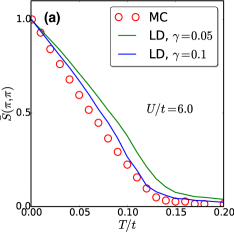
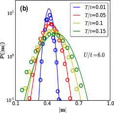
Figure 1: $\bar{S}(\pi,\pi)$ (a) and $P(|{\bf m}|)$ (b) for the square lattice Hubbard model at $U/t=6.0$. Solid lines denote answers obtained using the present LD method and open circles indicate MC data. We observe a reasonable agreement between the two methods.

III.1 Fixing the Langevin parameters

We do a bechmarking of the Langevin scheme using the square lattice as a test case. Three coupling regimes are explored- weak ($U/t=3.0$), intermediate ($U/t=6.0$) and strong ($U/t=10.0$). The statics is quantified through two quantities- the structure factor $S(\pi,\pi)$ and the moment magnitude distribution $P(|{\bf m}|)$. The former shows the correlation temperatures ($T_{corr}$), below which the correlation length approaches the system size. The latter details the longitudinal fluctuations of local moments. The alternate technique used to compute these quantities is a Monte Carlo calculation done assuming the auxiliary ${\bf m}_{i}$ field to be classical and using the sum of electronic free energy and the stiffness cost (last term in $H_{SF}$) as the sampling weight swain (see Appendix B for more details).

The method of fixing $\gamma$ was the following. We started with a low value (motivated by its vanishing magnitude at strong coupling, and the fact that we should get undamped spin waves at low enough $T$) at a fixed coupling and run length. Next, we increased the $\gamma$ at that coupling in steps till the match with MC results on temperature dependence became reasonable, while ensuring that the low $T$ spin waves remain sharp enough. Results for a typical coupling are quoted above.

Fig.1(a) shows a comparison of $\bar{S}(\pi,\pi)$ at $U/t=6$, with a reasonable match. The dissipative coefficients are $\gamma=0.05$ and $\gamma=0.1$. In Fig.1(b), the $P(|{\bf m}|)$ distributions also show reasonable agreement (for $\gamma=0.05$). We’ve used $\gamma=0.025$ to generate the bulk of our final dynamics results, which roughly corresponds to a relaxation timescale $\tau_{rel}\sim 40\tau_{mag}$. We will later quantify the increasing relevance of magnitude fluctuations on decreasing coupling, which is an important piece of the non-Heisenberg physics.

III.2 Magnetic scales for varying $U/t$

At low temperature, our dynamical equation (Eq.1) gives rise to weakly damped, dispersive spin wave excitations. From the obtained spectrum, we extract two scales- (i) the spin-wave stiffness, $J_{eff}$, and (ii) the magnon bandwidth, $W_{mag}$. The first is computed from the spin wave velocity of the linear branch near the respective Goldstone modes on the square and triangular lattice. The latter requires knowledge of the full magnon band structure. We plot these quantities for both the square and triangular lattice in Fig.2.

In Fig.2(a), we find a monotonic decrease of $J_{eff}$ with $U/t$ in the square lattice case, with a $1/U$ asymptote at strong coupling. The value at $U/t=20.0$ matches the expected $J_{eff}=4t^{2}/U$, indicating that one has reached the Heisenberg limit. On the triangular lattice, the stiffness goes to zero for $U/t=6.0$, indicating a breakdown of the $120\degree$ ordered state. The scale then rises and finally falls as $\sim 1/U$ at strong coupling. In Appendix C, we compare the extracted spin wave velocities with those obtained from RPA singh1 .

The magnon bandwidths Fig.2(b) feature a non-monotonicity in the square case, with a maximum around $U/t=6.0$. $W_{mag}$ increases on lowering $U$ on the triangle, rising to $0.6t$ before the ordered state breaks down.

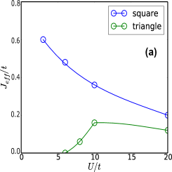
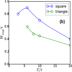
Figure 2: (a): The dimensionless effective exchange ($J_{eff}/t$), calculated from the spin wave velocity, for the square and triangular lattice Hubbard models at various $U/t$ values. We see a monotonic behaviour for the square lattice and a non-monotonic behaviour for the triangular lattice case. Moreover, the scale vanishes around $U/t=6.0$ for the latter, signalling a breakdown of $120\degree$ order. (b):The spin wave bandwidth ($W_{mag}$), calculated from the full magnon dispersion, for the square and triangular cases. Here, we see a non-monotonicity in the square lattice, and a gradual decrease in the triangular lattice.

III.3 Comparison with Heisenberg as $U/t\rightarrow\infty$

We compare the Hubbard results at $U/t=20$ on the square lattice with the Heisenberg model with $J=1$. The former effectively reduces to the latter with $J_{eff}=4t^{2}/U$ and $|{\bf m}_{i}|=1/2$. First, in 3(a), the low $T$ dispersions are compared, with both being scaled by $W_{mag}$, the spin wave bandwidth. There’s a nearly perfect agreement.

The Heisenberg model features three broad thermal regimes. These are- (i) weakly damped ($T\ll J$), where we obtain dispersive excitations with low damping, (ii) strongly damped ($T\sim{\cal O}(J)$), where there’s significant mode coupling among spin waves, but dispersion is still discernable, and (iii) diffusive ($T\gg J$), where mode frequencies collapse to zero and the dampings are comparable to $W_{mag}$. In these regimes, we compare the lineshapes of the Heisenberg model at ${\bf q}=(\pi/2,\pi/2)$ with those of the large $U$ Hubbard model in Fig.3(b). In regime (i), a sharp lineshape centered around $\Omega_{\bf q}=4J$ is seen, which picks up significant damping in regime (ii), before becoming diffusive in (iii). A quantitative agreement is seen between the Hubbard and Heisenberg results. The frequencies are scaled by $J_{eff}$ in the Hubbard case, and $J$ in the Heisenberg one.

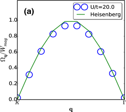
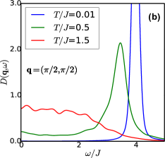
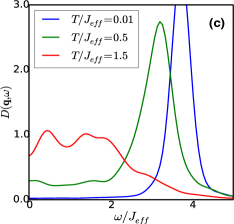
Figure 3: (a): Comparison of dispersions $\Omega_{\bf q}$ along the $K-\Gamma$ direction of the Brillouin Zone (BZ) between the square lattice Hubbard model at $U/t=20.0$ and the Heisenberg model with $J=1$. One gets a near perfect agreement on scaling the former by $J_{eff}=4t^{2}/U$. (b),(c): Lineshapes at three characteristic temperatures $T/J=0.01,0.5,1.5$ for the Heisenberg model (in (b)) and the $U/t=20.0$ Hubbard model (in (c)). There’s again a marked agreement.

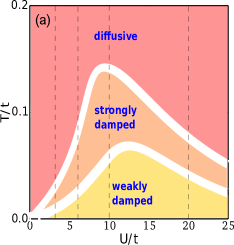
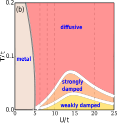
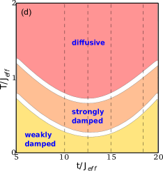
Figure 4: Magnon phase diagrams for square ((a) and (c)) and triangular ((b) and (d)) lattice Hubbard models at half-filling. The top row features the $U/t-T/t$ phase diagrams, while the bottom one exhibits the $T/J_{eff}-t/J_{eff}$ plots. We broadly observe three ”dynamical regimes”- (i) weakly damped (where $\Gamma_{\bf q}\lesssim 0.2W_{mag}$), (ii) ”strongly damped” (where $\Gamma_{\bf q}\sim{\cal O}(W_{mag})$) and (iii) ”diffusive” (where $\Gamma_{\bf q}\sim{\cal O}(W_{mag})$ and $\Omega_{\bf q}\rightarrow 0$). The metallic region in (b) is not tackled by our approach. Vertical sections indicate couplings used in actual simulations.

III.4 General features of dynamics in the Mott phase

We first comment on the broad dynamical regimes obtained on the square and triangular lattice problems. This is characterized by the the number of peaks, their location, and width.

As mentioned earlier, we find three broad dynamical regimes on analyzing the data- (i) weakly damped, where the linewidth for a generic momentum $\Gamma_{\bf q}\ll W_{mag}$, (ii) strongly damped, where $\Gamma_{\bf q}\sim{\cal O}(W_{mag})$ and (iii) diffusive, where $\Gamma_{\bf q}\sim{\cal O}(W_{mag})$ and $\Omega_{\bf q}\rightarrow 0$.

On the square lattice (Figs.4(a) and 4(c)), the low $T$ lineshapes are unimodal. There is a gradual crossover to regimes (ii) and (iii) at $T^{cr}_{1}(U)$ and $T^{cr}_{2}(U)$ respectively. The window of regime (ii) is maximum around $U/t=6.0$. The crossover lines behave $\sim 1/U$ asymptotically, but have a maximum around $U/t=10.0$. Below this coupling, the amplitude fluctuation effect dominates and consequent excess thermal dampings cause a downward trend. This non-Heisenberg feature is much better highlighted in 2(c), where both $T^{cr}_{1}/J_{eff}$ and $T^{cr}_{2}/J_{eff}$ decrease markedly on lowering $U$. At weak coupling, both these scales collapse quickly.

The loss of antiferromagnetic correlations at finite temperature is characterized through a temperature scale $T_{corr}$, extracted from $S(\pi,\pi)$. The crossover lines have a similarity to the locus of this $T_{corr}(U)$ tiwari , which also coincides with the metal-insulator transition line at weak coupling. However, there are quantitative differences. the peak location in our dynamical phase diagram Fig.4(a) is at $\sim U/t=10$, a higher coupling compared to the peak location in $T_{corr}$ at $\sim U/t=4$. We emphasize that our focus is on the ”local moment” regime, i.e, intermediate to strong coupling. Our method can address the weak coupling Slater regime as well but that regime is dominated by amplitude fluctuations and also requires larger system size.

In Section VI (subsection C), we discuss an effective classical moment model which actually interpolates between the Heisenberg and Slater limits, borrowing a few parameters from the Hubbard mean field and RPA results. This captures the low temperature dynamics of the Hubbard problem fairly well at all $U/t$, and the Heisenberg limit at all temperatures. Moreover, the non-monotonicity of $T_{corr}$ as a function of $U/t$ and the qualitative behaviour of the thermal regimes are also captured by the effective model.

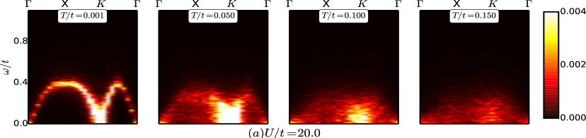
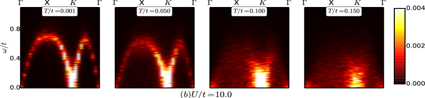
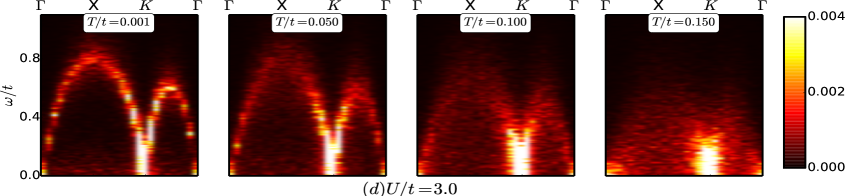
Figure 5: Power spectrum of magnetization field $D({\bf q},\omega)$ for the Hubbard model on the square lattice for $U/t=20,10,6,3$ respectively. The trajectory chosen in Brillouin Zone is $\Gamma-X-K-\Gamma$. Temperatures are scaled by electron hopping $t$. We observe a resemblance of the strong coupling Hubbard spectrum with that of the Heisenberg model with $J_{eff}=4t^{2}/U$. At lower couplngs, the dispersion changes at low $T$, owing to longer-range spin couplings. Thermal damping is more prominent at weaker couplings, as the stiffness for amplitude fluctuation decreases.

In the triangular case (Fig.4(b) and 4(d)), the generic low $T$ lineshapes is two-peak. The crossover regimes (ii) and (iii) occur at much lower temperatures compared to the square case, owing to mild geometric frustration and consequently fragile magnetic order. The fall of the crossover scales on decreasing $U$ (below $U/t=10.0$, say) is also sharper than the former. Close to the transition ($U/t\sim 6$) the lineshapes become diffusive even at very low temperatures ($T/t\sim 0.01$). The scaled phase diagram (4(d)) reveals a minimum in the crossover scales around $t/J_{eff}\sim 12.5$. This is related to the non-monotonic behaviour of $J_{eff}$ itself, shown in Fig.2.

We comment that our scheme at weak coupling generates a peak centered at zero frequency for all momenta, exclusively due to amplitude fluctuations. This arises from an oversimplification of our equations of motion. However, the fraction of this weight isn’t visible on a linear scale above $U/t\sim 4$ on the square. Moreover, if we ignore the near-zero energy part of the magnon spectrum (upto some cutoff $\sim 0.05W_{mag}$), the rest of it doesn’t have any spurious features. We still capture the impact of magnitude fluctuations on the damping of spin waves, which reside at higher energies.

Next, we present detailed numerical results on the dynamics of square and triangular lattice Hubbard models found using our scheme. The focus is on deviations from the Heisenberg limit, quantified through finite temperature behaviour of the damping of spin waves.

IV Dynamics on the square lattice

In this section, we first show the spectral maps of $D({\bf q},\omega)$ across a section of the Brillouin Zone (BZ) for four representative couplings, starting from the Heisenberg limit. Next, we extract the mode energies and magnon damping from the data and plot their variation with respect to $T$ and ${\bf q}$ respectively. Finally, a comparison of actual lineshapes for a generic wavevector ${\bf q}=(\pi/2,\pi/2)$ is featured.

IV.1 Spectral maps for varying $U/t$ and temperature

The dynamical structure factor maps are exhibited in Fig.5. The top row shows results for a $U/t=20.0$ Hubbard model (the Heisenberg limit) in various temperature regimes. The first column corresponds to the lowest $T$. Here, we see sharply defined spin waves, with Goldstone modes at both $(0,0)$ and $(\pi,\pi)$ and a characteristic antiferromagnetic dispersion. At intermediate temperatures ($T/t=0.05$), the bandwidth reduces and the spin waves broaden. On further increase in $T$, the correlations weaken to give a diffusive spectrum, with prominent low-energy weight close to $(\pi,\pi)$. Ultimately, the momentum dependence is also lost for $T/t=0.15$.

The lower panels show results on the Hubbard model for three successively lower couplings- strong ($U/t=10.0$), intermediate ($U/t=6.0$) and weak ($U/t=3.0$) respectively. At strong coupling, the behaviour is Heisenberg-like, with $J_{eff}\sim t^{2}/U$, with small deviations. The spectrum remains mostly coherent till $T\sim J_{eff}$, with momentum dependent thermal damping. The Goldstone mode at $(\pi,\pi)$ survives as a broad low-energy feature till $T\sim 2J_{eff}$.

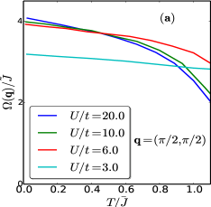
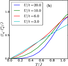
Figure 6: Fitted dispersions ($\Omega_{\bf q}$) and intrinsic thermal dampings ($\Gamma_{\bf q}-\Gamma^{0}_{\bf q}$) as functions of $T$, extracted from the dynamical spectra in the square lattice. The temperature axes are scaled by ${\bar{J}}=J_{eff}|{\bf m}_{HF}|^{2}$, while the frequencies are scaled by ${\tilde{J}}=J_{eff}|{\bf m}_{HF}|$ values for the various couplings studied. The dispersions soften slowly with increasing $T$, while one clearly observes the onset of non-Heisenberg behaviour in (b) for lower $U$ values, with large dampings showing up much below $T/{\bar{J}}=1$.

At intermediate coupling ($U/t=6.0$), the bandwidth increases compared to the earlier case and the low $T$ dispersion changes in shape. This owes its origin to the emergence of multi-spin couplings. There’s also a faint, momentum-independent low-energy band, more clearly visible in a logarithmic color scale. This band arises from longitudinal fluctuations of moments within our scheme, which is controlled by the local stiffness. Thermal fluctuations broaden the spin waves gradually, with the dispersion being discernable even at $T\sim 0.1t$.

The bottom row features weak coupling ($U/t=3.0$) results, where the low energy band gains more weight (now visible on a linear scale) and the bandwidth shortens again. Thermal effects are stronger, as amplitude fluctuations are more prominent here.

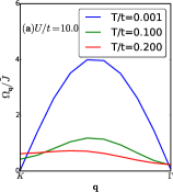
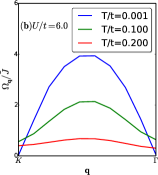
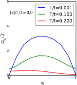
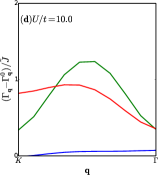
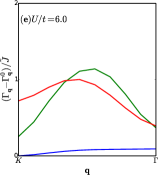
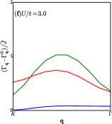
Figure 7: Fitted dispersions ($\Omega_{\bf q}$) in (a)-(c) and intrinsic thermal dampings ($\Gamma_{\bf q}-\Gamma^{0}_{\bf q}$) in (d)-(f), plotted against ${\bf q}$ along the $K-\Gamma$ trajectory in three thermal regimes- (i) weakly damped, (ii) strongly damped and (iii) diffusive. The couplings chosen are $U/t=3,6,10$ and the absolute temperatures are $T/t=0.001,0.1,0.2$. We observe a non-monotonicity in the peak frequency, and a mild shift of this peak to lower ${\bf q}$ on heating up. The bottom row reveals a residual momentum dependence of magnon damping even in the diffusive regime.

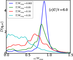
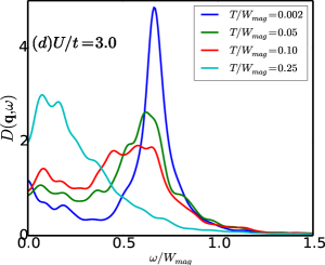
Figure 8: Lineshapes at ${\bf q}=(\pi/2,\pi/2)$ for the Hubbard model (a-d) for $U/t=20,10,6,3$ respectively. We see a clear deviation from Heisenberg-like behaviour in the thermal trends on decreasing coupling. Frequencies and temperatures are scaled by the respective bandwidths ($W_{mag}$) of the magnetization spectrum.

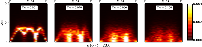
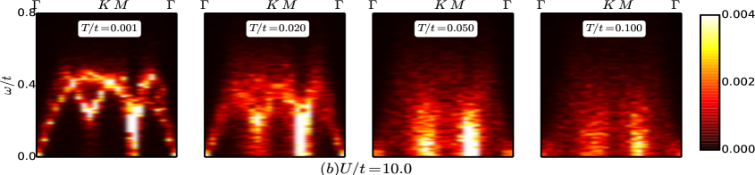
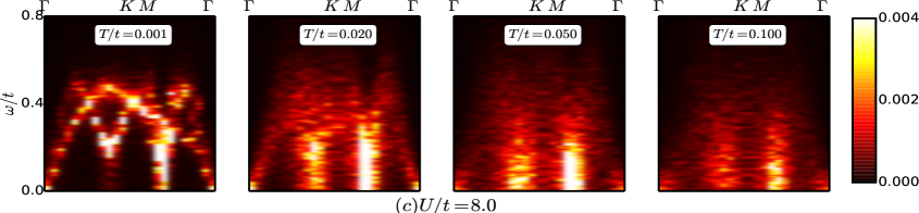
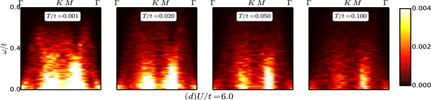
Figure 9: Power spectrum of magnetization field $D({\bf q},\omega)$ for the Hubbard model on the triangular lattice for $U/t=20,10,8,6$ respectively. The trajectory chosen in Brillouin Zone is $\Gamma-K-M-\Gamma$. Temperatures are scaled by electron hopping $t$. Again, we observe a similarity of the strong coupling Hubbard spectrum with the Heisenberg case. The lower branch between $\Gamma-K$ in the Heisenberg limit develops a prominent dip for lower $U$ values. The thermal dampings are stronger on moving to weaker couplings compared to the square case.

IV.2 Variation of mode energy and damping with $T$

Fig.6 highlights the evolution of mean frequency ($\Omega_{\bf q}$) and thermally induced linewidth ($\Gamma_{\bf q}-\Gamma^{0}_{\bf q}$) with temperature at a generic wavevector ${\bf q}=(\pi/2,\pi/2)$. The former monotonically falls with increasing $T$, as seen in 6(a). The rate of decrease speeds up around successively lower fractions of ${\tilde{J}}=J_{eff}|{\bf m}_{HF}|$ on moving to lower couplings. In 6(b), we see that the rise in thermal damping has an initially quadratic trend at large $U$ and low $T$, which then changes to a linear one one moving to lower couplings, and becomes $T^{\alpha}$ with $1<\alpha<2$ on raising $T$. A somewhat sharper fall is seen in the ”onset temperature” for strongly damped behaviour on lowering $U/t$, compared to the trend followed by the mean.

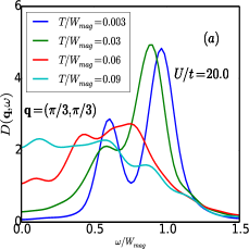
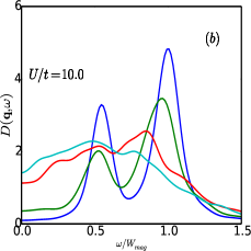
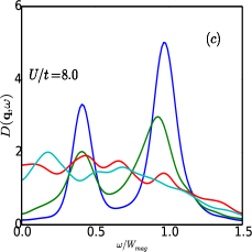
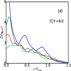
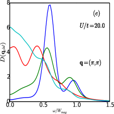
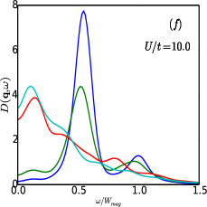
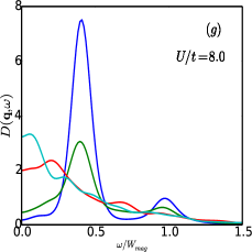
Figure 10: Triangular lattice: lineshapes at ${\bf q}=(\pi/3,\pi/3)$ (a-d) and ${\bf q}=(\pi,\pi)$ (e-h) for the Hubbard model for $U/t=20,10,6,3$ respectively. We see a clear deviation from Heisenberg-like behaviour in the thermal trends on decreasing coupling. Frequencies and temperatures are scaled by the respective bandwidths ($W_{mag}$) of the magnetization spectrum.

IV.3 Momentum dependence of energy and damping with changing temperature

In Fig.7, we concentrate on the momentum dependence of the same two quantities in the three broad thermal regimes, discussed before. We firstly see a monotonic behaviour of the peak frequency (at ${\bf q}=(\pi/2,\pi/2)$), as well as the finite $T$ bandwidth (scaled by $\tilde{J}$), on lowering $U$ in the weakly damped regime. The linewidths here are very small. In the strongly damped regime (green curves), the peak location of mean frequency shifts to slightly lower ${\bf q}$ at weak coupling, while the peak in magnon damping shifts towards higher ${\bf q}$ values. Finally, even in the diffusive regime, a residual momentum dependence can be observed in the linewidth plots ((d)-(f)).

IV.4 Lineshapes on the square lattice

Fig.8 highlights the behaviour of a specific high-momentum lineshape (at ${\bf q}=(\pi/2,\pi/2)$) as a function of frequency for several temperatures. Fig.8(a) is the Heisenberg limit ($U/t=20.0$) result. We see sharp mode gradually broadening and developing a tail-like feature upto $T/W_{mag}=0.1$ on increase in $T$. Finally, a diffusive lineshape emerges at high temperature ($T/W_{mag}=0.25$). The plots for $U/t=10.0$ shares most of these qualitative features. However, the extent of broadening at intermediate temperatures is much more at the same scaled temperatures for $U/t=6.0$. There’s a zero frequency feature for weaker couplings, most prominent for $U/t=3.0$. As discussed already, this is an artifact of the present method and shouldn’t be taken seriously.

We next move on to an example of a weakly frustrated system, the Hubbard model on the isotropic triangular lattice. This system has a finite $U_{c}\sim 4.5t$ and features 120°ordered ground states for $U\gtrsim 6t$. We focus our attention to the latter coupling regime. First, the spectral maps are exhibited, followed by lineshapes at two specific momenta.

V Dynamics on the triangular lattice

V.1 Spectral maps for varying $U/t$ and temperature

Fig.9 exhibits the spectral maps for the triangular lattice, in the same layout as in the square case. The four couplings represent ”Heisenberg” ($U/t=20.0$), ”strong” ($U/t=10.0$), ”intermediate” ($U/t=8.0$) and ”close to the transition” ($U/t=6.0$) regimes. The non-Heisenberg features like amplitude fluctuations and multi-spin couplings increase column-wise.

The spectrum in the Heisenberg limit is much more complicated than in the square case, as the background order corresponds to ${\bf q}=(2\pi/3,2\pi/3)$ due to the effect of mild frustration. We plot the spectrum along $\Gamma-K-M-\Gamma$ trajectory in the Magnetic Brillouin Zone (MBZ). There are two bands at a generic wavevector. The magnetic order is fragile, as indicated by the reduced bandwidth compared to the square case. Even on mild increase in $T$ ($T/W_{mag}=0.2$), the multi-band structure becomes fuzzy and large linewidths develop in the $M-\Gamma$ region. Further increase in $T$ makes most of the spectrum incoherent, apart from the Goldstone mode at the ordering wavevector.

Moving to the lower coupling counterparts, the strong coupling spectrum at low $T$ is similar to the Heisenberg result, with $J_{eff}\sim t^{2}/U$. The dip near $M$ point is more prominent. Thermal effects are also Heisenberg-like. On decreasing the coupling to $U/t=8.0$, the curvature of the $\Gamma-K$ branch increases at low $T$, as does the dip. Amplitude fluctuations induce more dramatic damping of the spin-wave modes at comparable temperatures. Finally, close to the Mott transition ($U/t=6.0$), even the low-$T$ spectrum is incoherent. Soft modes are visible in a wide region of momentum space. In Appendix D, we show the gradual evolution of the low temperature spectrum as one approaches the Mott transition, staying within the 120°ordered family of states.

V.2 Lineshapes on the triangular lattice

Fig.10 elaborates the comparison of detailed lineshapes of the Hubbard model with those of the Heisenberg in the triangular case. The two rows feature lineshapes for ${\bf q}=(\pi/3,\pi/3)$ and ${\bf q}=(\pi,\pi)$ respectively. Once again, the frequencies and temperatures are scaled with respect to the low $T$ bandwidth. The leftmost columns represent the Heisenberg limit ($U/t=20$) results. We observe that for both wavevectors, a bimodal spectrum is obtained at low $T$, which gradually broadens on increasing temperature. Even upto $T/W_{mag}\sim 0.1$, the spectra retain two distinct peaks.

Moving to the Hubbard results, we see that the strong coupling results ($U/t=10.0$) bear a striking resemblance to the Heisenberg case, as expected. However, even at moderately high coupling ($U/t=8.0$), the thermal damping results in diffusive behaviour even at $T/W_{mag}\sim 0.05$. On going closer to the Mott transition ($U/t=6.0$), even the low $T$ lineshapes significantly change their character, with prominent zero frequency weights cropping up in both the wavevectors. Diffusive behaviour sets in immediately on increasing $T$.

VI Discussion

We have tried to organise the results in this paper in terms of three dynamical regimes and then quantified the detailed response on these regimes in terms of the lineshape, the mode energy and the damping. In what follows we shall try to provide the analytic basis of some of the results seen in the Langevin simulations, also point out some of the limitations of our approach. The main effect observed in this paper is the enhancement of thermal damping of magnons as one moves away from the Heisenberg limit. We argue this effect maybe minimally captured by a simpler classical toy model, which allows for amplitude fluctuations and approaches the classical Heisenberg limit upon tuning a single parameter.

VI.1 Classification of non-Heisenberg effects at finite $U/t$

We first comment that there exists a two-particle continuum of excitations, originating from particle-hole processes, missed out by the present scheme. This is accessed by a quantum RPA calculation done on the mean-field ordered states on square and triangular geometries. However, this continuum is energetically well separated from the spin wave spectrum at strong coupling and hence don’t influence each other at the temperature scales of interest. But, this argument breaks down at weak coupling (e.g. $U/t=3.0$), where indeed there’s appreciable mixing even at low temperature, and our dynamical results are indeed imperfect, except near special, symmetry-protected wavevectors like $(0,0)$ or $(\pi,\pi)$. In what follows, we only underline the non-Heisenberg features observed in the spin wave part.

In the full Hubbard problem, at intermediate $U/t$ values, there are two main non-Heisenberg features- (i) the ordered state and the low $T$ dispersion are modified, and (ii) the moment magnitudes are no longer fixed but are reduced at low $T$ and also fluctuate thermally. We’ll discuss the impact of the second class of features in detail in the upcoming subsections. To obtain the effects of the first class systematically at low $T$, one does an expansion about the mean-field state, which may (as in the square lattice case) or may not (as in the triangular one) have the same ordering as in the Heisenberg limit, with a reduced moment value. The effective Hamiltonian for ${\bf m}_{i}$’s, obtained through integrating out the electrons perturbatively in $t/U$, now involves longer range, multi-spin terms capriotti ; yang . The couplings are decided by the electronic band structure on the mean field state. However, we should remember that our model is composed of classical moments. Hence, the coefficients don’t match with those in the actual quantum model.

These coefficients depend non-trivially on $U/t$. As a result, the crossover lines between the thermal regimes are modified with respect to the Heisenberg case.

To lowest order, a linear theory maybe written down for the fluctuations, which has an analytic solution. We’ll discuss this subsequently in subsection C. The contribution to the effective field ($\frac{\partial<H>}{\partial{\bf m}_{i}}$) coming from the leading non-Heisenberg term, expanded upto ${\cal O}(\delta{\bf m}_{i})$ in fluctuations, looks like-

$$\sum_{ijkl}K_{ijkl}({\bf m}^{0}_{j}({\bf m}^{0}_{k}.\delta{\bf m}_{l}+\delta{\bf m}_{k}.{\bf m}^{0}_{l})+\delta{\bf m}_{j}({\bf m}^{0}_{k}.{\bf m}^{0}_{l}))$$

The coupling $K_{ijkl}$ has a lowest order contribution of ${\cal O}(t^{4}/U^{3})$, as maybe motivated from a perturbative argument, starting from the strong coupling limit. One now puts this expression back in the first and second terms of Eq.1, along with the Heisenberg term $4t^{2}/U\sum_{<j>}{\bf m}_{j}$ and the stiffness contribution ($U(|{\bf m}_{i}|-1/2)^{2}$), and solves the resulting equation via Fourier transformation. From the poles of the ensuing power spectrum, one gets the low $T$ dispersion, which contains the leading non-Heisenberg effects.

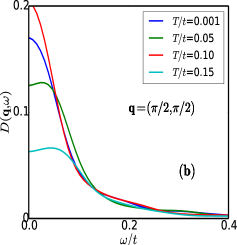
Figure 11: (a): Fitted standard deviations ($\Delta|{\bf m}|$) from $P(|{\bf m}|)$ distributions, plotted against temperature for three couplings in the square lattice case. Blue open circles denote actual data points, while solid lines are fits using a square root function. The trends indicate the increasing importance of amplitude fluctuations at weaker couplings and a square root dependence, expected of a ”soft spin” Heisenberg model. (b): Lineshapes at ${\bf q}=(\pi/2,\pi/2)$ for the amplitude fluctuations at $U/t=6.0$, indicating a diffusive mode centered at zero energy.

VI.2 Quantifying amplitude fluctuations

In this subsection, we quantify the extent and intrinsic dynamical signature of fluctuations in the moment magnitude, before launching into the construction of an effective model to describe them. Fig.11(a) focusses on the longitudinal fluctuations of the magnetic moments. These are, of course, frozen in the Heisenberg limit. We fit the $P(|{\bf m}|)$ distributions, shown earlier in Fig.1, to Gaussians and extracted the corresponding standard deviations. These are plotted as functions of temperature for various coupling values in the square lattice case. In a ”soft spin” Heisenberg model, where the intersite term is Heisenberg but longitudinal fluctuations are allowed, the behaviour should be $\sim\sqrt{T}$. However, we observe deviations from this trend at lower $U$ values. The coefficient of the square root fits is exactly $1/\sqrt{U}$ at strong coupling. Even at weaker couplings, the deviations are small. Hence, the amplitude fluctuations can be effectively captured by a local term $H_{amp}=\sum_{i}U(|{\bf m}_{i}|-1/2)^{2}$.

The spectral signature of these fluctuations is a diffusive mode centered at zero frequency, shown in Fig.11(b). This is obvious from the locality of $H_{amp}$, which deactivates the torque term in Eq.1. The width is regulated by $\gamma$. Interestingly, the weight at low frequency shows a non-monotonic behaviour with $T$. This behaviour, however, doesn’t capture the true physics of the amplitude mode, which should have a signature at $\omega\sim U$. For that, one needs to incorporate quantum fluctuations of the magnetization field in the effective equation of motion. We’ll discuss this briefly in subsection E.

VI.3 Construction of an effective model

In the following, we describe the construction of an effective ”classical moment” model, which essentially captures the qualitative features of the full Hubbard model calculation at all $U/t$. The model reads-

$$H_{eff} = J_{eff}\sum_{<ij>}{\bf m}_{i}.{\bf m}_{j}+\frac{K_{eff}}{2}\sum_{i}(|{\bf m}_{i}|-|{\bf m}_{HF}|)^{2}$$ (9)

$$-2J_{eff}\sum_{i}|{\bf m}_{i}|^{2}$$

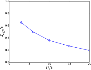
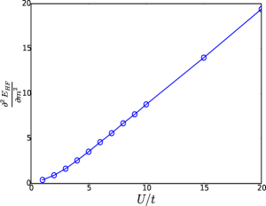
Figure 12: The effective exchange $J_{eff}$, second derivative of Hartree-Fock energy with respect to moment magnitude ($\frac{\partial^{2}E_{HF}}{\partial{m}^{2}}$), which is proportional to the amplitude stiffness $K_{eff}$ and Hartree-Fock moment value ($|{\bf m}_{HF}|$), as determined from HF and RPA calculations, for various $U/t$ values on the square lattice Hubbard model.

The first term encapsulates an ”effective” nearest neighbour exchange between the local moments ${\bf m}_{i}$, the second term is an amplitude stiffness which regulates the thermally induced fluctuations of the moment magnitude and the third term is a counterterm that fixes the low $T$ moment size to exactly $|{\bf m}_{HF}|$, the Hartree-Fock value. The parameters $J_{eff}$ and $K_{eff}$ are extracted, respectively, from the low $T$ RPA spin wave velocity (fitted to a nearest-neighbour Heisenberg model) and the “curvature” of the Hartree-Fock energy, ${\partial^{2}E_{HF}}/{\partial{m}^{2}}$. Fig.12 illustrates the behaviour of the above parameters for various $U/t$ values.

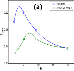
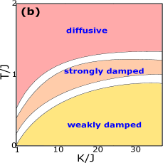
Figure 13: Left: Comparison of the correlation temperatures ($T_{corr}$), extracted from the respective structure factors $S(\pi,\pi)$ of the full Hubbard (blue curves) and effective model (green curves) obtained using Monte Carlo (MC) method described in the paper. One observes that the non-monotonicity is well captured by the former model. Right: Thermal regimes obtained using Langevin dynamics of the effective model (Eq.10) with varying $K/J$. A qualitative resemblance with the square lattice Hubbard results (Fig.4(c)) is apparent.

The model is constructed based on a strong coupling expansion argument. At large $U/t$, the Hubbard model reduces to a spin model of the following form-

$$H_{eff} = H_{loc}+H_{coup}$$ (10)

$$H_{loc}~{} = U(|{\bf m}_{i}|-\frac{1}{2})^{2}+...$$ (12)

$$H_{coup} = J_{2}\sum_{<ij>}{\bf m}_{i}.{\bf m}_{j}+J_{4}\sum_{ijkl}f[{\bf m}_{i},...{\bf m}_{l}]+...$$ (14)

$H_{loc}$ is basically the HF energy in terms of moment magnitude, expanded to quadratic order in the deviations. $H_{coup}$ reduces to the first term with $J_{2}=4t^{2}/U$ as $U/t\rightarrow\infty$. This can be shown explicitly by expanding about the $U/t\rightarrow\infty$ local limit. On including further terms in the expansion (subleading in $t/U$), one gets longer range, multi-spin couplings. We lump the effect of all non local terms into an equivalent nearest neighbour coupling $J_{eff}$ and retain the local amplitude stiffness in our simplified model. The strong coupling limit is also correctly recovered as $J_{eff}\rightarrow 4t^{2}/U$, $K_{eff}\rightarrow 2U$ and $|{\bf m}_{i}|\rightarrow 1/2$ as $U/t\rightarrow\infty$ in our model. The result of the aforesaid construction is that it reproduces the thermal physics of the classical Heisenberg model at all $T/t$ for large $U/t$. At weaker couplings, the $T=0$ state is captured with the correct (mean-field) moment value and the low-energy spin wave excitations (in particular their velocity $v_{SW}$) are also correctly captured by construction.

     

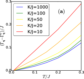
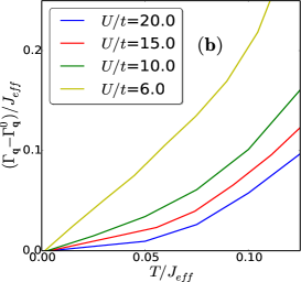
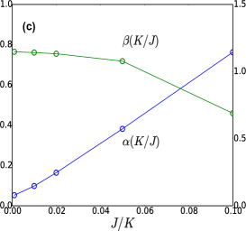
Figure 14: (a): The excess thermal damping ($\Gamma_{\bf q}-\Gamma^{0}_{\bf q}$), plotted as a function of $T/J$ for various stiffness values in the approximate $J-K$ model for ${\bf q}=(\pi/2,\pi/2)$. One notes that the low $T$ linear regime shrinks on increasing $K/J$ and the behaviour turns to parabolic. (b): The same quantity extracted from the full Hubbard model calculation at various $U/t$ values. Similar qualitative features are observed. (c): Plot of fitting parameters $\alpha$ and $\beta$ for the approximate model, showing the quadratic to linear crossover on decreasing $K/J$.

As regards the results obtained using the above model, we first compare the static indicators, in particular the low temperature structure factor $S(\pi,\pi)$ between the original Hubbard model and this effective model at various $U/t$ values. To minimize parametric dependencies, the comparison was done using the Monte Carlo technique, elaborated in Appendix B. The results for the correlation temperatures ($T_{corr}$) are shown in Fig.13(a). The basic observation is that the non-monotonicity of this scale as a function of $U/t$, is succesfully captured by the effective model, albeit the maximum is slightly shifted to higher $U/t$. The $T_{corr}$ within the effective model scales roughly as $\sim|{\bf m}|_{HF}^{2}J_{eff}$ for large $U/t$, but crashes faster at lower $U$ due to the effect of $K_{eff}$.

To further simplify the three parameter effective model of Eq.8, we scaled the effective couplings $J_{eff}$ and $K_{eff}$ by the moment value $|{\bf m}_{HF}|$ appropriately and reduced Eq.8 to an ”equivalent one-parameter” model of the following form-

$$H_{1par}=J\sum_{<ij>}{\bf m}_{i}.{\bf m}_{j}+\frac{K}{2}\sum_{i}(|{\bf m}_{i}|-1)^{2}-2J\sum_{i}|{\bf m}_{i}|^{2}$$ (15)

where $J$ is set to 1 and $K/J$ is varied to mimic the behaviour of the earlier model. The moment magnitudes fluctuate about unity for all couplings in this model. The results obtained using Eq.10 agree quantitatively with those originating from Eq.8, which is formally equivalent.

Next, we move to the dynamics. The thermal regimes in the dynamics of the effective model (Eq.10) are depicted in Fig.13(b). They qualitatively resemble the scaled phase diagram (Fig.4(c)) of the full Hubbard problem. This corroborates the usefulness of the effective model, not only to understand the static properties, but also dynamical features.

After comparing the gross features of the dynamics, we also examined whether the same effective model (Eq.10) can mimic the changing low $T$ behaviour of the damping in the full Hubbard problem. We extracted the excess damping at finite $T$ and plotted it for the generic ${\bf q}=(\pi/2,\pi/2)$ as a function of $T/J$. One finds that empirically one may fit this excess damping $\Gamma_{\bf q}-\Gamma^{0}_{\bf q}$ to a polynomial of the form $\alpha T+\beta T^{2}$, with the coefficients depending on $K/J$.

Upon examining the fitting parameters, one observes that the $\alpha\propto 1/K$ at low $K$ and decreases to zero in the fixed moment limit ($K/J\rightarrow\infty$). The quadratic coefficient $\beta$ is roughly constant at large $K$. The results are shown in Fig.14(a) and 14(c). Such features are also observed qualitatively in the full Hubbard calculation, where the normalizing energy scale is chosen as $J_{eff}=4t^{2}/U$. These results are shown in Fig.14(b).

We next try to find an a posteriori justification for the rising linear coefficient and rise in damping as on reduces the amplitude stiffness by imagining undamped spin wave modes getting affected by amplitude disorder. If one is at sufficiently low temperature, the equation of motion (Eq.1) maybe linearized in terms of deviation from the ground state configuration. On the square lattice, for instance, one simply expands the ${\bf m}_{i}$ as

$${\bf m}_{i} = {\bf m}^{0}_{i}+\delta{\bf m}_{i}$$ (16)

$${\bf m}^{0}_{i} = (-1)^{i_{x}+i_{y}}\hat{z}$$ (17)

Keeping upto the linear order in fluctuations $\delta{\bf m}_{i}$ gives us an analytically solvable starting point. The effective equation is-

$$\frac{d\delta{\bf m}_{i}}{dt} + J({\bf m}^{0}_{i}\times\sum_{<j>}\delta{\bf m}_{j}-\sum_{<j>}{\bf m}^{0}_{j}\times\delta{\bf m}_{i})$$ (18)

$$+ \gamma(J\sum_{<j>}\delta{\bf m}_{j}+K\sum_{i}(-1)^{i}\delta m^{z}_{i}\hat{z})={\vec{\xi}}_{i}$$ (19)

The transverse and longitudinal modes gets decoupled at this order. On Fourier transforming this equation and solving for the power spectrum, one finds the usual dispersion of the antiferromagnetic classical Heisenberg model, while the damping of transverse spin wave modes is limited by $\gamma J$. The longitudinal modes generally give rise to a diffusive lineshape, and freeze for $K/J\rightarrow\infty$. On top of this low temperature, purely transverse theory, one may switch-on amplitude fluctuations perturbatively. The width of these fluctuations is $\propto 1/K$. On treating them as static, uncorrelated disorder, they cause the eigenmodes of the linear theory to scatter. In the lowest order Born approximation, this generates a self-energy, whose imaginary part translates to an additional contribution to the magnon linewidth. This has a prefactor $T$ coming from the propagator of transverse fluctuations. In the static limit, the coefficient of this correction is thus proportional to $T/K$. Hence as $K$ is reduced from infinity, the linear $T$ correction to spin wave damping increases as $1/K$, as is seen in the numerical data.

The aforesaid argument doesn’t include the effect of non-linear interactions among the transverse fluctuations. To evaluate their effect, one expands upto second order in the deviation field, which generates a $\delta{\bf m}_{\bf q}\times\delta{\bf m}_{\bf q^{\prime}}$ contribution in the equation of motion. If one substitutes the lowest order solution in this and averages over the noise, this correction term vanishes, owing to the fact that the noise is uncorrelated between different Cartesian axes. Hence, no $O(T)$ contribution is found for the damping of transverse fluctuations. The lowest order correction is of ($O(T^{2})$), as is found in the extensive literature harris ; tyc . This becomes the leading term when amplitude fluctuations are completely restricted (in the $K/J\rightarrow\infty$ limit).

VI.4 Computational issues for frustrated systems

One would want to ultimately apply this formalism to study the Hubbard model on fully frustrated geometries (e.g. Kagome in 2d and pyrochlore in 3d). The rich spin dynamics, with the moment softening and multipsin coupling effects present beyond the Heisenberg limit, should be accessible at finite temperature. However, there are some tough computational difficulties associated with this attempt. Briefly, the issues are-

• Extracting even the static properties correctly (vis-a-vis Monte Carlo) requires much longer run lengths compared to the square or triangular case. This occurs due to the rugged free energy landscape associated with the problem. Novel strategies, involving simultaneous updation of multiple moments, ameliorate the situation in specific cases.

• The numerical implementation of the Langevin dynamics scheme, using Suzuki-Trotter decomposition, breaks down when the systematic torque on a site becomes identically zero. This happens, for instance, for the Heisenberg model on the 2d Kagome lattice. Hence, a more complicated discretization strategy is called for.

VI.5 Adiabaticity and thermal noise

VI.5.1 The adiabatic assumption

Our approach has assumed that the characteristic timescale for magnetic fluctuations is much greater than electronic timescales, in analogy with the electron-phonon problem sauri . In such a situation (i) the electronic energy depends only on the instantaneous magnetic configuration, and (ii) the leading contribution to electronic correlators can be computed without invoking retardation effects. This argument holds good in the strong coupling regime, where the magnetic fluctuations operate on a scale of $J_{eff}\sim t^{2}/U$ and the electrons are gapped at a scale $\sim U$. However, as $U/t$ reduces, the former scale rises and the latter diminishes due to closing of the gap. So, the argument isn’t very good. We also comment that the auxiliary field correlator, which we computed, reproduces the essential features of the real spin-spin correlator $\langle{\bf\sigma}_{i}(t).{\bf\sigma}_{j}(t^{\prime})\rangle$, measured in INS experiments as long as the adiabaticity assumption holds good. This happens because the auxiliary field dynamics basically follows the ${\bf\sigma}_{i}$ field, with the distinction that its magnitude is not strictly bounded between 0 and 1. As a result, the respective intensities are different.

VI.5.2 The noise driving the dynamics

The present method for accessing spin dynamics excludes the effect of quantum fluctuations. This firstly results in the unphysical freezing of the moments at $T=0$ and makes the method unable to access the ground state magnon spectrum. Furthermore, this feature limits the viability of the scheme at low temperatures for frustrated geometries, where order by disorder phenomena are observed. To remedy this, the noise has to be consistently generated with respect to the polarizability of the problem, which itself will depend on the ${\bf m}_{i}(t)$ trajectories.

Using a Keldysh formulation of the original Hubbard model, and decomposing the interaction term using an auxiliary vector field ${\bf m}_{i}$, we may subsequently assume this field to be slow with respect to the electrons. This enables one to write an effective equation of motion for ${\bf m}_{i,cl}$ of the following form-

$$\Im\left[Tr\left(\hat{G}^{K}_{ii}(t,t)\vec{\sigma}\right)\right] = {\bf m}_{i,cl}(t)+\vec{\xi}_{i}(t)$$

$$\langle\xi^{a}_{i}(t)\xi^{b}_{j}(t^{\prime})\rangle = \left[\hat{\Pi}^{K}(t,t^{\prime})\right]^{ab}_{ij}$$ (20)

Here $G^{K}$ and $\Pi^{K}$ are the Keldysh Green’s function and (spin-dependent) polarizability of the electrons respectively. In the adiabatic limit, each of these maybe expanded in a Kramers-Moyal series arijit . On assuming that the coefficients don’t have any spatial dependence and the temperature is high enough compared to characteristic frequency scale of these, one arrives at a much simpler equation of the LLG form, which upon neglecting certain multiplicative noise terms reduces to Eq.1.

To include the effect of quantum fluctuations, the high $T$ approximations done on the coefficients of the Kramers-Moyal expansion need to be relaxed. Basically, if the temperature approaches the energy scale of two-particle excitations, the memory-less assumption on the noise becomes unjustified.

VII Conclusions

We’ve studied the dynamics of magnetic moments in the Mott insulating phase of the half-filled Hubbard model on square and triangular lattice geometries, using a Langevin dynamics based real time technique. The method reproduces known results on the Heisenberg model in the strong coupling limit, and the RPA based low-energy dispersion at low $T$ faithfully. We observe three broad regimes in the dynamics- (i) weakly damped, where spin waves are dispersive and dampings are small, (ii) strongly damped, where one can see significant broadening due to mode coupling, but the dispersive character survives, and (iii) diffusive, where the mode frequencies collapse to zero and the dampings span the full bandwidth. The main results are twofold- (a)  we obtain the deviation of low temperature dispersion from the Heisenberg results, and (b) we observe the onset of the thermal crossovers at significantly lower values of $T/J_{eff}$, compared to the Heisenberg case. One also captures the effect of mild geometric frustration on the mode damping, on going from the square to the triangle. The method maybe applied to study equilibrium dynamics in fully frustrated lattices (e.g. pyrochlore) in near future.

We acknowledge use of the High Performance Computing Facility at HRI.

Appendix A: Numerical details of the Langevin scheme

All of our Langevin dynamics simulations are done by discretizing Eq.1 in real time and implemented in a Cartesian coordinate scheme. The particular technique used to solve the equations is the Euler-Maruyama method euler . The time step is chosen to be $0.01\tau_{mag}$. At each step, the derivatives appearing in the RHS of Eq.1 are computed through exact diagonalization of the electronic problem. The derivative $\frac{\partial\langle H_{SF}\rangle}{\partial{\bf m}_{i}}$ for our model is just $U({\bf m}_{i}-\langle{\bf\sigma}_{i}\rangle)$. Typically, the simulations are ran for $3\times 10^{6}$ steps. We gave parallel runs for each temperature point, with the Hartree-Fock (HF) state as the initial condition for each value of the Hubbard coupling. The lattice size for the results shown for both the square and triangular cases is $18\times 18$.

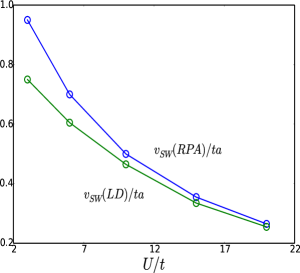
Figure 15: Comparison of spin wave velocities ($v_{SW}$) computed using our Langevin dynamics (LD) technique and the random phase approximation (RPA) on the square lattice. We observe similar trends and quantitatively lower values in LD compared to RPA. This is due to our assumption of classical spins.

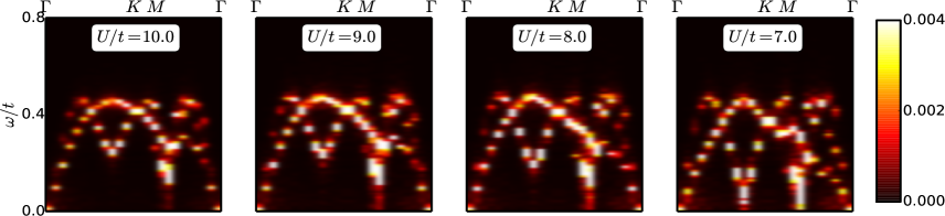
Figure 16: Low temperature spectra on the triangular lattice on gradually lowering $U$, approaching the Mott transition. All the couplings shown display order at zero temperature, with progressively smaller moment magnitudes. One observes a dramatic softening of modes along the $\Gamma-K$ region in momentum space, albeit with a robust magnon bandwidth.

Appendix B: Numerical details of the Monte Carlo scheme

To benchmark the static properties obtained via the Langevin scheme, we used a competing Monte Carlo (MC) method. One first writes the Hubbard model in the Matsubara formalism and then decouples the quartic interaction in terms of the ${\bf m}_{i}$ field. Next, only the zero Matsubara mode of this field is retained, assuming $T\gtrsim J_{eff}$ and temporal fluctuations of the field can be neglected. However, the thermal fluctuations and the associated spatial correlations are treated non-perturbatively. This enables one to write an effective Hamiltonian for the auxiliary fields as-

$$H_{eff} = -\frac{1}{\beta}logTre^{-\beta H_{el}}+U\sum_{i}|{\bf m}_{i}|^{2}$$ (21)

$$H_{el} = -\sum_{<ij>\sigma}t_{ij}(c^{\dagger}_{i\sigma}c_{j\sigma}+h.c.)-U\sum_{i}{\bf m}_{i}.{\bf\sigma}_{i}$$

Finally, configurations of the ${\bf m}_{i}$ field are sampled using $P({\bf m}_{i})=Tr_{cc^{\dagger}}e^{-\beta H_{eff}}$ as the sampling weight. These configurations are used for computing static structure factors and distribution of moment magnitudes, defined in Eq.5 and Eq.7 respectively and shown in Fig.1(a) and 1(b). We also mention that the correlation temperatures in 2(a) are size-dependent, and will ultimately collapse logarithmically with system size. However, we’ve still compared the MC and Langevin answers for the same system size to ensure that the latter method faithfully reproduces the static properties.

Appendix C: Comparison of low temperature spectrum with RPA

We compare the low temperature spectra obtained using our technique with the standard spin wave theory (RPA) results for the square lattice in Fig.15. The spin wave velocities are quoted from the work of Singh et. al. singh1 . One observes a fair agreement in terms of the trends. The RPA values are slightly higher. We ascribe this discrepancy to our assumption of classical magnetic moments. However, since our main focus is on the finite temperature dynamics, the quantitative mismatch isn’t very important. The agreement improves as one approaches the Heisenberg limit.

Appendix D: Approaching the Mott transition

In the triangular lattice, there’s a finite $U_{c}\sim 4.5t$ for the Mott transition. Close to the transition, one observes complex large-period order hrk . However, staying within the 120°ordered state (restricting ourselves to large enough $U/t$ values where the ground state is the former), we observe signatures of proximity to $U_{c}$ in the spectrum. Fig.16 shows a marked softening of magnetic modes along the $\Gamma-K$ trajectory and a gradual linear trend of the dispersion along $K-M$ as the coupling is lowered. We’ve already shown the spectra at $U/t=6$ in the main text, which is the lowest coupling we’ve explored within the 120°ordered family. Ideally, the complex dynamics in the vicinity of the transition should also be capturable using our strategy, but requires considerably more numerical effort, as one needs to do a thermal annealing to even fix the initial state for the dynamics.

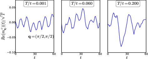
Figure 17: Real time trajectories of $Re(m^{z}_{\bf q})(t)$ in three thermal regimes- (i) weakly damped ($T/t=0.001$), (ii) strongly damped ($T/t=0.06$) and (iii) diffusive ($T/t=0.2$). In (i), we see oscillations with timescale $\sim\tau_{mag}$ In (ii), some intermediate timescales emerge, but the earlier scale is still visible. In (iii), the bare-oscillation scale is obliterated and slow, large amplitude fluctuations dominate.

Appendix E: Real time dynamics

In Fig.17, we show the trajectory of the real part of $m^{z}_{\bf q}$ for a generic wavevector, ${\bf q}=(\pi/2,\pi/2)$, in real time for the three representative regimes- (i) weakly damped, (ii) strongly damped and (iii) diffusive. These are results for the square lattice Hubbard model at $U/t=10.0$. We’ve also scaled the y-axis by $\sqrt{T}$, to gauge out the dominant part of amplitude fluctuations. At the lowest $T$, we see oscillatory behaviour, modified by weak noise. The characteristic timescale is $\tau_{mag}\sim 1/J_{eff}$. This corresponds to a well-defined lineshape in frequency. In the second panel (regime (ii)), one observes the emergence of some new timescales, but the earlier scale is still visible. This translates in frequency space to broadened lineshapes centered around $\Omega_{\bf q}(T=0)$. On heating up further, thermal effects kill off the bare-oscillation timescale and slow oscillations dominate the time series. The amplitude also increases significantly, even after gauging the $\sqrt{T}$ factor.

References

- [1] X. Y. Zhang, M. J. Rozenborg, and G. Kotliar, Phys. Rev. Lett. 70, 1666 (1993).
- [2] Masatoshi Imada, Atsushi Fujimori, and Yoshinori Tokura, Rev. Mod. Phys. 70, 1039 (1998).
- [3] Marcelo J. Rozenberg, R. Chitra, and Gabriel Kotliar, Phys. Rev. Lett. 83, 3498 (1999).
- [4] Massimo Capone, Luca Capriotti Federico Becca, and Sergio Caprara, Phys. Rev. B 63, 085104 (2001).
- [5] H. Park, K. Haule, and G. Kotliar, Phys. Rev. Lett. 101, 186403 (2008).
- [6] Takuma Ohashi, Tsutomu Momoi, Hirokazu Tsunetsugu, and Norio Kawakami, Phys. Rev. Lett. 100, 076402 (2008).
- [7] Peyman Sahebsara and David Sénéchal, Phys. Rev. Lett., 100, 136402 (2008).
- [8] A. Yamada, Phys. Rev. B 89, 195108 (2014).
- [9] Takuma Ohashi, Norio Kawakami, and Hirokazu Tsunetsugu, Phys. Rev. Lett. 97, 066401 (2006).
- [10] Yuta Furukawa, Takuma Ohashi, Yohta Koyama, and Norio Kawakami, Phys. Rev. B 82, 161101(R) (2010).
- [11] N. Bulut, W. Koshibae, and S. Maekawa, Phys. Rev. Lett. 95, 037001 (2005).
- [12] A. Yamada, K. Seki, R. Eder, and Y. Ohta, Phys. Rev. B 83, 195127 (2011).
- [13] Tomoko Kita, Takuma Ohashi, and Norio Kawakami, Phys. Rev. B 87, 155119 (2013).
- [14] Satoshi Fujimoto, Phys. Rev. B 64, 085102 (2001).
- [15] B. Normand and Z. Nussinov, Phys. Rev. Lett. 112, 207202 (2014).
- [16] Nyayabanta Swain, Rajarshi Tiwari, and Pinaki Majumdar, Phys. Rev. B 94, 155119 (2016).
- [17] J. E. Hirsch, Phys. Rev. B 31, 4403 (1985).
- [18] S. R. White, D. J. Scalapino, R. L. Sugar, E. Y. Loh, J. E. Gubernatis, and R. T. Scalettar, Phys. Rev. B 40, 506 (1989).
- [19] H. R. Krishnamurthy, C. Jayaprakash, Sanjoy Sarker, and Wolfgang Wenzel, Phys. Rev. Lett. 64, 950 (1990).
- [20] Walter Zimmermann, Raymond Fresard, and Peter Wolfle, Phys. Rev. B 56, 10097 (1997).
- [21] Hal Tasaki, J. Phys. Condens. Matter 10, 4353 (1998).
- [22] Patrick Fazekas, Lecture notes on Electron Correlations and Magnetism, World Scientific (1999).
- [23] S. Hochkeppel, F. F. Assaad, and W. Hanke, Phys. Rev. B 77, 205103 (2008).
- [24] T. Watanabe, H. Yokoyama, Y. Tanaka, and J. Inoue, Phys. Rev. B 77, 214505 (2008).
- [25] Takuya Yoshioka, Akihisa Koga, and Norio Kawakami, Phys. Rev. Lett. 103, 036401 (2009).
- [26] Luca F. Tocchio, Helene Feldner, Federico Becca, Roser Valenti, and Claudius Gros, Phys. Rev. B 87, 035143 (2013).
- [27] Luca F. Tocchio, Claudius gros, Roser Valenti, and Federico Becca, Phys. Rev. B 89, 235107 (2014).
- [28] J. Kokalj and Ross H. McKenzie, Phys. Rev. Lett. 110, 206402 (2013).
- [29] Shimpei Goto, Susumu Kurihara, and Daisuke Yamamoto, Phys. Rev. B 94, 245145 (2016).
- [30] Tomonori Shirakawa, Takami Tohyama, Jure Kokalj, Sigetoshi Sota, and Seiji Yunoki, Phys. Rev. B 96, 205130 (2017).
- [31] Shaozhi Li and Emanuel Gull, Phys. Rev. Research 2, 013295 (2020).
- [32] A. Georges, G. Kotliar, W. Krauth, and M.J. Rozenberg, Rev. Mod. Phys. 68, 13 (1996).
- [33] R. Bulla, Phys. Rev. Lett. 83, 136 (1999).
- [34] Rok Zitko, Janez Bonca, and Thomas Pruschke, Phys. Rev. B 80, 245112 (2009).
- [35] Martin Eckstein, Marcus Kollar, and Philipp Werner, Phys. Rev. B 81, 115131 (2010).
- [36] Robert Peters and Norio Kawakami, Phys. Rev. B 89, 155134 (2014).
- [37] Motoharu Kitatani, Naoto Tsuji, and Hideo Aoki, Phys. Rev. B 92, 085104 (2015).
- [38] Gabriel Kotliar and Andrei E. Ruckenstein, Phys. Rev. Lett. 57, 1362 (1986).
- [39] H. J. Schulz, Phys. Rev. Lett. 65, 2462 (1990).
- [40] Chang-Ming Ho, V. N. Muthukumar, Masao Ogata, and P. W. Anderson, Phys. Rev. Lett. 86, 1626 (2001).
- [41] Avinash Singh and Zlatko Tesanovic, Phys. Rev. B 41, 614 (1990).
- [42] Avinash Singh and Zlatko Tesanovic, Phys. Rev. B 41, 11457 (1990).
- [43] Avinash Singh, Phys. Rev. B, 71, 214406 (2005).
- [44] O. Gunnarsson, T. Schafer, J.P.F. LeBlanc, E. Gull, J. Merino, G. Sangiovanni, G. Rohringer, and A. Toschi, Phys. Rev. Lett. 114, 236402 (2015).
- [45] Gia-Wei Chern, Kipton Barros, Zhentao Wang, Hidemaro Suwa and Cristian D. Batista, Phys. Rev. B 97, 035120 (2018).
- [46] J. P. F. LeBlanc, Shaozhi Li, Xi Chen, Ryan Levy, A. E. Antipov, Andrew J. Millis, and Emanuel Gull, Phys. Rev. B 100, 075123 (2019).
- [47] Charles L. Cleveland and Rodrigo Medina A., Am. J. Phys., 44, 44 (1976).
- [48] R. E. Watson, M. Blume, and G. H. Vineyard, Phys. Rev. 181, 180 (1969).
- [49] M. Blume and J. Hubbard, Phys. Rev. B 1, 3815 (1970).
- [50] Minoru Takahashi, J. Phys. Soc. Jpn. 52, 3592 (1983).
- [51] M. E. Gouvêa, G. M. Wysin, A. R. Bishop, and F. G. Mertens, Phys. Rev. B 39, 11840 (1989).
- [52] A. R. Völkel, G. M. Wysin, A. R. Bishop, and F. G. Mertens, Phys. Rev. B 44, 10066 (1991).
- [53] P. Peczak and D. P. Landau, Phys. Rev. B 47, 14260 (1993).
- [54] J. E. R. Costa and B. V. Costa, Phys. Rev. B 54, 994 (1996).
- [55] R. Moessner and J. T. Chalker, Phys. Rev. Lett. 80, 2929 (1998).
- [56] Mathieu Taillefumier, Julien Robert, Christopher L. Henley, Roderich Moessner, and Benjamin Canals, Phys. Rev. B 90, 064419 (2014).
- [57] Nicholas E. Sherman and Rajiv R. P. Singh, Phys. Rev. B 97, 014423 (2018).
- [58] Luca Capriotti, Andreas Lauchli, and Arun Paramekanti, Phys. Rev. B 72, 214433 (2005).
- [59] Hong-Yu Yang, Andreas M. Lauchli, Frederic Mila, and Kai Phillip Schmidt, Phys. Rev. Lett., 105, 267204 (2010).
- [60] G. Aeppli, S. M. Hayden, H. A. Mook, Z. Fisk, S.-W. Cheong, D. Rytz, J. P. Remeika, G. P.Espinosa, and A. S. Cooper, Phys. Rev. Lett. 62, 2052 (1989).
- [61] R. Coldea, S. M. Hayden, G. Aeppli, T. G. Perring, C. D. Frost, T. E. Mason, S.-W. Cheong, and Z. Fisk, Phys. Rev. Lett. 86, 5377 (2001).
- [62] C. Stock, R. A. Cowley, W. J. L. Buyers, C. D. Frost, J. W. Taylor, D. Peets, R. Liang, D. Bonn, and W. N. Hardy, Phys. Rev. B 82, 174505 (2010).
- [63] Y. Kurosaki, Y. Shimizu, K. Miyagawa, K. Kanoda, and G. Saito, Phys. Rev. Lett. 95, 177001 (2005).
- [64] B. J. Powell and Ross H. McKenzie, Rep. Prog. Phys. 74, 056501 (2011).
- [65] O. Friedt, P. Steffens, M. Braden, Y. Sidis, S. Nakatsuji, and Y. Maeno, Phys. Rev. Lett. 93, 147404 (2004).
- [66] P. Steffens, O. Friedt, Y. Sidis, P. Link, J. Kulda, K. Schmalzl, S. Nakatsuji, and M. Braden, Phys. Rev. B 83, 054429 (2011).
- [67] M. C. Shapiro, Scott C. Riggs, M. B. Stone, C. R. de la Cruz, S. Chi, A. A. Podlesnyak, and I. R. Fisher, Phys. Rev. B 85, 214434 (2012).
- [68] S. K. Choi, R. Coldea, A. N. Kolmogorov, T. Lancaster, I. I. Mazin, S. J. Blundell, P. G. Radaelli, Yogesh Singh, P. Gegenwart, K. R. Choi, S.-W. Cheong, P. J. Baker, C. Stock, and J. Taylor, Phys. Rev. Lett. 108, 127204 (2012).
- [69] Keisuke Tomiyasu, Kazuyuki Matsuhra, Kazuaki Iwasa, Masanori Watahiki, Seishi Takagi, Makoto Wakeshima, Yukio Hnatsu, Makoto Yokoyama, Kenji Ohoyama, and Kazuyoshi Yamada, J. Phys. Soc. Jpn. 81, 034709 (2012).
- [70] S. Bahr, A. Alfonsov, G. Jackeli, G. Khaliullin, A. Matsumoto, T. Takayama, H. Takagi, B. Buchner, and V. Kataev, Phys. Rev. B 89, 180401(R) (2014).
- [71] Wei Bao, C. Broholm, M. Honig, P. Metcalf, and S. F. Trevino, Phys. Rev. B 54, 3726(R) (1996).
- [72] Young-June Kim, A. P. Sorini, C. Stock, T. G. Perring, J. van den Brink, and T. P. Devereaux, Phys. Rev. B 84, 085132 (2011).
- [73] Chih-Wei Chen, Weiyi Wang, Vaideesh Loganathan, Scott V. Carr, Leland W. Harriger, C. Georgen, Andriy H. Nevidomskyy, Pengcheng Dai, C. -L. Huang, and E. Morosan, Phys. Rev. B 99, 144423 (2019).
- [74] R. Blankenbecler, D. J. Scalapino, and R. L. Sugar, Phys. Rev. D 24, 2278 (1981).
- [75] G. Kotliar, S. Y. Savrasov, K. Haule, V. S. Oudovenko, O. Parcollet, and C. A. Marianetti, Rev. Mod. Phys. 78, 865 (2006).
- [76] Vu Hung Dao and Raymond Fresard, Phys. Rev. B 95, 165127 (2017).
- [77] J.P.F. LeBlanc, Andrey E. Antipov, Federico Becca, Ireneusz W. Bulik, Garnet Kin-Lic Chan, Chia-Min Chung, Youjin Deng, Michel Ferrero, Thomas M. Henderson, Carlos A. Jiménez-Hoyos, E. Kozik, Xuan-Wen Liu, Andrew J. Millis, N.V. Prokof’ev, Mingpu Qin, Gustavo E. Scuseria, Hao Shi, B.V. Svistunov, Luca F. Tocchio, I.S. Tupitsyn, Steven R. White, Shiwei Zhang, Bo-Xiao Zheng, Zhenyue Zhu, and Emanuel Gull (Simons Collaboration on the Many-Electron Problem), Phys. Rev. X 5, 041041 (2015).
- [78] Pui-Wai Ma and S. L. Dudarev, Phys. Rev. B 86, 054416 (2012).
- [79] A. Kirilyuk, A. V. Kimel, and T. Rasing, Rev. Mod. Phys. 82, 2731 (2010).
- [80] A. Rebei and G. J. Parker, Phys. Rev. B 67, 104434 (2003).
- [81] William Fuller Brown, Jr., Phys. Rev. 130, 1677 (1963).
- [82] A. Rebei, W. N. G. Hitchon, and G. J. Parker 72, 064408 (2005).
- [83] B. Mera, V. R. Vieira, and V. K. Dugaev, Phys. Rev. B 88, 184419 (2013).
- [84] Rajarshi Tiwari’s thesis (2013). http://www.hri.res.in/ libweb/theses/softcopy/rajarshi-tiwari.pdf
- [85] A. B. Harris, D. Kumar, B. I. Halperin, and P. C. Hohenberg, Phys. Rev. B 3, 961 (1971).
- [86] Stéphane Ty and Bertrand I. Halperin, Phys. Rev. B 42, 2096 (1990).
- [87] Sauri Bhattacharyya, Sankha Subhra Bakshi, Samrat Kadge, and Pinaki Majumdar, Phys. Rev. B 99, 165150 (2019).
- [88] Arijit Dutta, Pinaki Majumdar, arXiv 2009.04533 (2020).
- [89] P. E. Kloeden and E. Platen, Numerical Solution of Stochastic Differential Equations, Springer, Berlin (1992).