Regularization of the Nambu-Jona Lasinio model under a uniform magnetic field and the role of the anomalous magnetic moments

Abstract

The vacuum contribution to quark matter under a uniform magnetic field within the SU(3) version of the Nambu and Jona-Lasinio model is studied. The standard regularization procedure is examined and a new prescription is proposed. For this purpose analytic regularization and a subtraction scheme are used to deal with divergencies depending on the magnetic intensity. This scheme is combined with the standard three momentum cutoff recipe, and reduces to it for vanishing magnetic intensity. Furthermore, the effects of a direct coupling between the anomalous magnetic moments of the quarks and the magnetic field is considered. Single particle properties as well as bulk thermodynamical quantities are studied for a configuration of matter found in neutron stars. A wide range of baryonic densities and magnetic intensities are examined at zero temperature.

I Introduction

The study of dense matter under strong interaction is usually carried out by employing effective models, due to the intricacies of the fundamental theory . Within this approach, the Nambu-Jona Lasinio (NJL) model has shown to be a useful conceptual tool to tackle different problems. In particular, it has been widely used to describe quarks interacting with magnetic fields MIRANSKY ; ANDERSEN ; KLEVANSKY ; GUSYNIN ; EBERT ; FERRER ; NORONHA ; FROLOV ; CHATTERJEE ; DENKE ; FERRER2 ; AMAN ; PAIS . Within this versatile description a variety of issues have been analyzed such as magnetic catalysis, magnetic oscillations EBERT , color superconductivity FERRER ; NORONHA ; CHATTERJEE ; AMAN , chiral density waves FROLOV , vector DENKE and tensor FERRER2 additional couplings, and quark starsPAIS .
Multiple efforts have been made to extract physical content from the vacuum of the strong interaction affected by a magnetic field BLAU ; GOYAL ; ANDERSEN1 ; COHEN ; RUGGERI . Ref. BLAU provides general expressions for the effective action of a Dirac field interacting with a magnetic field for intensities greater than the mass scale. A description based on the chiral sigma lagrangian has been made in GOYAL , ANDERSEN1 uses the quark-meson model, whereas in COHEN the vacuum contribution to the magnetization is evaluated in a one-loop approach to QCD for very intense magnetic fields. Using the chiral quark model and a Ginzburg-Landau expansion Ref. RUGGERI has found that different treatments of the divergences could yield important modifications of the phase diagram.
The investigation of this issue has been particularly active within the NJL model KLEVANSKY ; GUSYNIN ; EBERT ; MENEZES ; FAYAZ2 ; ANDERSEN2 ; AVANCINI0 ; AVANCINI1 ; AVANCINI2 ; FAYAZ ; CHAUDHURI , since the contribution coming from the Dirac sea of quarks is responsible for the dynamical breaking of the chiral symmetry and it is a crucial point of the NJL model. There exist several prescriptions to deal with divergent contributions in the NJL at zero magnetic field, all of them yield compatible predictions. But it seems that it is not the case in the presence of an external magnetic field, as was recently pointed out in AVANCINI1 ; AVANCINI2 . In these references it is mentioned that the use of smooth form factors instead of a steep cutoff could change drastically the physical predictions. Particularly Ref. AVANCINI2 points out that a reliable regularization must clearly distinguish between the non-magnetic vacuum contribution from the magnetic one. A failure in this point should be the cause of the inadequate behavior found in different calculations, such as tachyonic poles in the spectrum of light mesons and unphysical oscillations in thermodynamical quantities.
Following the analytic regularization in terms of the Hurwitz zeta function BLAU , a residue depending on the squared magnetic intensity is found in EBERT . To dispose of this singularity, the authors propose a wavefunction renormalization by associating it to the pure magnetic contribution to the energy density. To deal with the divergencies in the thermodynamic potential, in MENEZES ; FAYAZ2 the pressure at zero baryonic density and finite $B$ is subtracted and added, in the former case still exhibiting the undesirable divergency and in the latter one it has been regularized in the 3-momentum cutoff scheme. While in the calculations of FAYAZ a softening regulator is used to analyze the effects of the AMM on the quark matter phase diagram, in CHAUDHURI a step function in momentum space is used with the same purpose.

An interesting aspect to be taken into account for Dirac particles in a magnetic field is the discrepancy of the gyromagnetic factor from the ideal value 2. This can happen in a quasiparticle scheme where the effects of some interactions give rise to the anomalous magnetic moments (AMM)SINGH ; BICUDO ; FERRER2 . As a reference one can take the prediction of the non relativistic constituent quark model for the magnetic moments of the light quarks. In order to adjust the experimental values of the proton and neutron magnetic moments, the gyromagnetic ratios $\tilde{g}_{u}=2\mu_{u}/\mu_{N}=3.7$, $\tilde{g}_{d}=2\mu_{d}/\mu_{N}=-1.94$ are obtained within this approach.
The appearance of AMM is closely related to the breakdown of the chiral symmetry. For this reason the NJL model with zero current quark mass have been used to study the origin of the AMM FERRER2 ; SINGH ; BICUDO . To analyze the feasibility of the dynamical generation of the AMM, in SINGH a one loop correction to the electromagnetic vertex is evaluated within the one flavor NJL model, obtaining

$$\tilde{g}\approx\frac{2M_{p}}{M}\frac{e_{q}}{e}\left[1-(M/\Lambda)^{2}\log(\Lambda/M)\right].$$

In a more sophisticated treatment they obtain $\tilde{g}_{u}\approx 3.72,\;\tilde{g}_{d}\approx-1.86$, by choosing adequately the constituent quark masses.
In the approach of BICUDO the AMM is extracted from the low momentum electromagnetic current written in terms of the kernel of the Ward identities. Assuming a four momentum cutoff, they find zero AMM in a one flavor NJL model. However, by using the two flavor version, the authors obtain $\tilde{g}_{u}\approx 3.813,\;\tilde{g}_{d}\approx-1.929$, which differ from the phenomenological expectations by less than $1\%$. Furthermore, in the same work an schematic confining potential for only one flavor is considered. By taking a constituent quark mass $M=330$ MeV, typical of the NJL model, the magnitude of the AMM predicted is as large as 0.15.
Another point of view is developed in FERRER2 , where the one flavor NJL model is supplemented with a four fermion tensor interaction, which induces a condensate in the $\gamma^{1}\,\gamma^{2}$ channel. In this case the intrinsic relation between the constituent quark mass and its AMM is explicitly exposed, since the vacuum condensate which breaks the chiral symmetry is also responsible for the occurrence of nonzero AMM. As a consequence, the AMM has a non-perturbative dependence on the magnetic intensity.
The necessity of the AMM of the quarks has been emphasized in MEKHFI in the context of the Karl-Sehgal formula, which relates baryonic properties with the spin configuration of the quarks composing them. By stating the dynamical independency of the axial and tensorial quark contributions to the baryonic intrinsic magnetism, the AMM of the quarks are proposed as the parameters that distinguish between them. Resorting to sound arguments, the author propose $a_{u}=a_{d}\approx 0.38$, $a_{s}\approx 0.2-0.38$ as significative values for the AMM for the lightest flavors.

Other investigations have focused on the consequences of a linear coupling between the AMM of the quarks and an external magnetic field FAYAZ ; CHAUDHURI ; GONZALEZ . For instance, FAYAZ analyze the phase diagram of the NJL at finite temperature, with special emphasis on a possible chiral restoration due to the non-zero AMM. Furthermore, the possibility of a non linear coupling of the AMM of the quarks is considered. In this model the AMM is related to the quantum correction to the electrodynamic vertex, and a non-perturbative dependence on the magnetic field is introduced through the effective constituent quark mass. The influence of the AMM on the structure of the lightest scalar mesons is analyzed in CHAUDHURI , while GONZALEZ is devoted to study their effects on neutral and beta stable quark matter within a bag model.

The aim of the present work is to study the effects of a uniform magnetic field on the properties of matter of quarks that have acquired AMM. In particular we focus on the vacuum effects and we perform an analytical regularization of the NJL that matches the standard three-momentum cutoff scheme for vanishing magnetic intensity. For this purpose, a fermion propagator is used which includes the anomalous magnetic moments and the full interaction with the external magnetic field AGUIRRE1 ; AGUIRRE2 . This propagator has been used to evaluate meson properties AGUIRRE2 ; AGUIRR3 , and the effect of the AMM within the NJL model CHAUDHURI . Previous investigations have considered quarks with AMM within this framework FAYAZ ; CHAUDHURI , but the divergent one-dimensional integrals were treated with a momentum cutoff which depends on the magnetic intensity. In the case of FAYAZ the cutoff parameter $\Lambda$ is inspired by a covariant 4-momentum scheme $E_{n\,s}(p,B)<\Lambda$, where $E_{n\,s}(p,B)$ represents the energy of the $n$-th Landau level with spin projection $s$ along the direction of the uniform magnetic field. Ref. CHAUDHURI , instead, uses a 3-momentum cutoff $p<\sqrt{\Lambda^{2}+M^{2}-E_{n\,s}(0,B)^{2}}$.
In the present work a 3-flavor version of the NJL is used. Most of the references just cited, in particular those corresponding to the study of AMM, use the two-flavor formulation. Thus we provide here an insight on the dynamics of the strange degree of freedom. This is particularly useful for applications to astrophysical studies, as for instance the final stage of neutron stars, where quark matter is electrically neutral and it is in equilibrium against weak decay.

This work is organized as follows. In the next section a summary of the NJL model is presented and a set of prescriptions to deal with the divergent contributions of the Dirac sea of quarks with AMM is proposed. Some numerical results are discussed in Sec. III, and the last section is devoted to drawing the conclusions.

II Effects of the AMM on the vacuum properties in the NJL model

The SU(3) NJL model extended with an AMM term has the Lagrangian density

$${\cal L}_{NJL}=\bar{\psi}\left(i/\!\!\!\!D-M_{0}-\frac{1}{2}\kappa\,\sigma_{\mu\,\nu}F^{\mu\,\nu}\right)\psi+G\left[\left(\bar{\psi}\lambda_{a}\psi\right)^{2}+\left(\bar{\psi}i\gamma^{5}\lambda_{a}\psi\right)^{2}\right]-K\left[\text{det}\,\bar{\psi}(1+\gamma^{5})\psi+\text{det}\,\bar{\psi}(1-\gamma^{5})\psi\right],$$

where a summation over color and flavor is implicit and the current mass matrix $M_{0}=\text{diag}(M_{0u},M_{0d},M_{0s})$ breaks explicitly the chiral symmetry and the covariant derivative $D^{\mu}=\partial^{\mu}-iQeA^{\mu}/3$ takes account of the uniform magnetic field, with $Q=\text{ diag}(2,-1,-1)$. The AMM are displayed in the matrix $\kappa=\text{ diag}(\kappa_{u},\kappa_{d},\kappa_{s})$ and the definition $\sigma_{\mu\nu}=i[\gamma_{\mu},\gamma_{n}u]/2$ is used. In the following only the zero temperature case is considered.

Due to the presence of a vacuum condensate the quark field acquires an enlarged constituent mass, a process that in the usual Hartree approach is described by

$$M_{i}=M_{0i}-4G\langle\bar{\psi}_{i}\psi_{i}\rangle+2K\langle\bar{\psi}_{j}\psi_{j}\rangle\langle\bar{\psi}_{k}\psi_{k}\rangle,$$ (1)

for $i\neq j\neq k$.

By using standard techniques KLEVANSKY ; KUNIHIRO ; VOGL one finds the grand partition function per unit volume $\Omega$,

$$\Omega=\sum_{f}\left[N_{c}\,T_{f}+2G\langle\bar{\psi}_{f}\psi_{f}\rangle^{2}\right]-4K\langle\bar{\psi}_{u}\psi_{u}\rangle\langle\bar{\psi}_{d}\psi_{d}\rangle\langle\bar{\psi}_{s}\psi_{s}\rangle.$$ (2)

In the limit of zero temperature the first term between square brackets can be decomposed as $T_{f}=T_{0f}-\mu_{f}\,n_{f}$, where $n_{f}$ stands for the particle number density for a given flavor $f$, and the Lagrange multipliers $\mu_{f}$ manifest the simultaneous conservation of the electric charge and the baryonic number. Alternatively, the kinetic contribution $T_{0f}$ can be expressed as $T_{0f}=\langle\bar{\psi}_{f}\,i\gamma^{0}\partial_{0}\,\psi_{f}\rangle$ KLEVANSKY and eventually can be evaluated in terms of the single particle Green function.
Both quantities $\langle\bar{\psi}_{k}\psi_{k}\rangle$ and $\langle\bar{\psi}_{k}i\gamma^{0}\partial_{0}\psi_{k}\rangle$ are ultraviolet divergent and need to be interpreted adequately. There are several standard recipes within the NJL model, such as the non-covariant 3-momentum cutoff and the Lorentz invariant procedures of Pauli-Villars and 4-momentum cutoff. In the present work a regularization procedure is used which reduces to the 3-momentum cutoff at vanishing magnetic field. For this purpose a fermionic propagator is used corresponding to an effective quark with constituent mass and interacting with an uniform magnetic field through the electric charge and the AMM. It has been deduced for positively charged fermions in AGUIRRE1 within the real time formalism of the thermal field theory Thermo Field Dynamics LANDSMAN . For the sake of completeness the results corresponding to zero temperature are transcribed here

$$G_{f}(x^{\prime},x)=e^{i\Phi}\int\frac{d^{4}p}{(2\pi)^{4}}e^{-ip^{\mu}\,(x^{\prime}_{\mu}-x_{\mu})}\left[G_{f0}(p)+e^{-p_{\bot}^{2}/\beta_{f}}\sum_{n,s}(-1)^{n}G_{fns}(p)\right]$$ (3)

where

$$G_{f0}(p) = e^{-p_{\bot}^{2}/\beta_{f}}\left(\not\!u+M_{f}-K_{f}\right)\left(1+i\gamma^{1}\gamma^{2}\right)\;\Xi_{0s},$$ (4)

$$G_{fns}(p) = \frac{\Delta_{n}+sM_{f}}{2\Delta_{n}}\Big{\{}(\not\!u-K_{f}+s\Delta_{n})\left(1+i\gamma^{1}\gamma^{2}\right)L_{n}(2p_{\bot}^{2}/\beta_{f})-(\not\!u+K_{f}-s\Delta_{n})$$ (5)

$$\times\left(1-i\gamma^{1}\gamma^{2}\right)\frac{s\Delta_{n}-M_{f}}{s\Delta_{n}+M_{f}}L_{n-1}(2p_{\bot}^{2}/\beta_{f})+\left(\not\!u\,i\gamma^{1}\gamma^{2}+s\Delta_{n}-K_{f}\right)\not\!v\frac{s\Delta_{n}-M_{f}}{p_{\bot}^{2}}$$

$$\times\left[L_{n}(2p_{\bot}^{2}/\beta_{f})-L_{n-1}(2p_{\bot}^{2}/\beta_{f})\right]\Big{\}}\;\Xi_{ns},$$

$$\Xi_{ns} = \frac{1}{p_{0}^{2}-E_{fns}^{2}+i\epsilon}+2\pi\,i\,n_{F}(p_{0})\,\delta(p_{0}^{2}-E_{fns}^{2}).$$ (6)

A similar expansion holds for negatively charged particles. In these expressions the index $s=\pm 1$ describes the spin projection on the direction of the uniform magnetic field. Eq. (4) propagates the lowest Landau level with the unique projection $s=1$ for the $u$ flavor and $s=-1$ for the $s,d$ cases. The sum over the index $n\geq 1$ takes account of the higher Landau levels, and the following notation is used $\beta_{f}=e|Q_{f}|B/3$, $K_{f}=\kappa_{f}\,B$, $\not\!u=p_{0}\gamma^{0}-p_{z}\gamma^{3}$, $\not\!v=-p_{x}\,\gamma^{1}-p_{y}\,\gamma^{2}$, $p_{\bot}^{2}=p_{x}^{2}+p_{y}^{2}$, $L_{m}$ stands for the Laguerre polynomial of order $m$, and

$$E_{fns} = \sqrt{p_{z}^{2}+(\Delta_{n}-s\,K_{f})^{2}}$$

$$\Delta_{n} = \sqrt{M_{f}^{2}+2n\beta_{f}}$$

Furthermore, $n_{F}(p_{0})=\Theta\left(\mu_{f}-E_{fns}\right)$ stands for the canonical statistical distribution function for fermions in thermodynamical equilibrium. Finally, the phase factor $\Phi=\beta_{f}(x+x^{\prime})(y^{\prime}-y)/2$ embodies the gauge fixing.

Using the propagator of Eq. (3) the quark condensates and the kinetic contributions are evaluated as KLEVANSKY

$$\langle\bar{\psi}_{f}\,\psi_{f}\rangle = -i\;\lim_{t^{\prime}\rightarrow t^{+}}\,\text{Tr}\{G_{f}(t,\vec{r},t^{\prime},\vec{r})\},$$ (7)

$$\langle\bar{\psi}_{f}\,i\gamma^{0}\partial_{0}\,\psi_{f}\rangle = -i\;\lim_{t^{\prime}\rightarrow t^{+}}\,\text{Tr}\left\{i\gamma^{0}\frac{\partial}{\partial t}\,G_{f}(t,\vec{r},t^{\prime},\vec{r})\right\},$$ (8)

together with

$$\langle\bar{\psi}_{f}\,\gamma^{\nu}\,\psi_{f}\rangle =-i\;\lim_{t^{\prime}\rightarrow t^{+}}\,\text{Tr}\{\gamma^{\nu}\,G_{f}(t,\vec{r},t^{\prime},\vec{r})\}.$$ (9)

The principle of thermodynamical consistency can be imposed through the relation $0=\partial\Omega/\partial M_{0f}$ BUBALLA .
As already mentioned, these quantities have divergent vacuum contributions. In the Appendix a regularization procedure is applied that ensures null vacuum contributions at zero magnetic intensity. This requisite is used to match the 3-momentum cutoff procedure, by simply adding the standard expressions in terms of the cutoff parameter $\Lambda$. Thus at the regularization point these quantities reduce to the commonly used vacuum values. But for any other conditions, finite contributions depending on the density and the magnetic intensity are extracted from the vacuum.
Eq. (9) represents the density of baryonic current, which for infinite homogeneous matter has zero vacuum value.
In the Appendix the derivation of the regularized Dirac sea terms of Eq. (8) is shown. That expression reduces to

$$\langle\bar{\psi}_{f}\,i\gamma^{0}\partial_{0}\psi_{f}\rangle^{\text{D}}-\langle\bar{\psi}_{f}\,i\gamma^{0}\partial_{0}\psi_{f}\rangle_{NJL} \rightarrow -\frac{N_{c}\beta_{f}^{2}}{2\pi^{2}}\left[\zeta^{\prime}\left(-1,x\right)-\frac{1}{2}\left(x^{2}-x+\frac{1}{6}\right)\ln(x)+\frac{\tilde{x}^{2}}{4}\right]+\frac{N_{c}\beta_{f}^{2}}{48\pi^{2}}$$ (10)

$$+ \frac{N_{c}\beta_{f}^{2}}{4\pi^{2}}\left(x^{2}+x+\frac{1}{6}\right)\ln\left(\frac{\nu}{M_{f}^{2}}\right)-\frac{N_{c}\beta_{f}^{2}}{4\pi^{2}}\left(3\tilde{x}^{2}-\tilde{x}+\frac{1}{6}\right)\ln\left(\frac{\nu}{\tilde{M}_{f}^{2}}\right)$$

for $\kappa_{f}\rightarrow 0$. The notation $x=M_{f}^{2}/(2\beta_{f})$ and $\tilde{x}=\tilde{M}_{f}^{2}/(2\beta_{f})$ has been used, where $\tilde{M}_{f}$ stands for the constituent mass at finite baryonic density and $B=0$. In this form, it can be compared with previous results, as for instance EBERT

$$-\frac{N_{c}\beta^{2}}{2\pi^{2}}\left[\zeta^{\prime}\left(-1,x\right)-\frac{1}{2}\left(x^{2}-x\right)\ln(x)+\frac{x^{2}}{4}\right]$$

The first term of Eq. (10) resembles the last equation. However, they differ in two points. First, the polynomial multiplying the logarithm has an extra term, which comes from the definition of $\zeta(-1,x)$. Furthermore in the last term between square brackets the quantities $\tilde{M}$ and $M$ are taken as identical. The remaining terms of Eq. (10) are missing in the mentioned approach. The difference can be minimized by choosing $\nu=M_{f}^{2}$. In such case, the third term of Eq.(10) becomes null, and the last one would also be zero if one identifies $\tilde{M}=M$. For this reason we adopt in the following $\nu=M_{f}^{2}$, but the distinction between $M_{f}$ and $\tilde{M}_{f}$ will be kept.

Furthermore, Eqs. (7)-(9) receives finite contributions from the Fermi sea

$$\langle\bar{\psi}_{f}\psi_{f}\rangle^{\text{F}} = \frac{N_{c}}{2\pi^{2}}\beta_{f}M_{f}{\sum_{n,s}}^{\prime}\frac{\Delta_{n}-sK_{f}}{\Delta_{n}}\ln\left(\frac{\mu_{f}+p_{fns}}{\Delta_{n}-sK_{f}}\right),$$ (11)

$$\langle\bar{\psi}_{f}\,i\gamma^{0}\partial_{0}\psi_{f}\rangle^{\text{F}} = \frac{N_{c}}{2\pi^{2}}{\sum_{n,s}}^{\prime}\left[\mu_{f}\,p_{fns}+\left(\Delta_{n}-sK_{f}\right)^{2}\ln\left(\frac{\mu_{f}+p_{fns}}{\Delta_{n}-sK_{f}}\right)\right],$$ (12)

$$n^{\nu}_{f}=\langle\bar{\psi}_{f}\gamma^{\nu}\psi_{f}\rangle^{\text{F}} = \delta_{\nu 0}\frac{N_{c}}{6\pi^{2}}\beta_{f}{\sum_{n,s}}^{\prime}p_{fns},$$ (13)

where the primed sum indicates that for $n=0$ only one spin projection must be considered as explained previously. The highest occupied Landau level N is defined by the condition $\mu_{f}^{2}-(\Delta_{N}-sK_{f})^{2}\geq 0$. The Lagrange multipliers $\mu_{f}$ are determined by the conserved charges, and $p_{fns}=\sqrt{\mu_{f}^{2}-(\Delta_{N}-sK_{f})^{2}}$.

The magnetization per unit volume is given by the equation ${\cal M}=-\partial\Omega/\partial B$, which can be simplified by using the stationary point conditions BRODERICK ; AVANCINI0 ,

$${\cal M}=\frac{N_{c}}{8\pi^{2}B}\sum_{f}\left({\cal D}_{f}+2\,\beta_{f}{\sum_{n,s}}^{\prime}{\cal F}_{ns}\right),$$

where

$${\cal D}_{f} = 8\beta_{f}^{2}\,\zeta^{\prime}\left(-1,\omega_{f}\right)-2\beta_{f}\left[M_{f}^{2}-K_{f}^{2}\right]\,\ln\left(\frac{\Gamma\left(\omega_{f}\right)}{\sqrt{2\pi}}\right)-\left[2K_{f}^{2}\left(K_{f}^{2}+M_{f}^{2}-\beta_{f}\right)-\beta_{f}\left(M_{f}^{2}+K_{f}^{2}-\frac{\beta_{f}}{3}\right)\right]\,\ln\left(\frac{M_{f}}{2\beta_{f}}\right)$$ (14)

$$+ 2\beta_{f}\left(M_{f}+K_{f}\right)\left(M_{f}+3K_{f}\right)\ln\left(1+\frac{K_{f}}{M_{f}}\right)-4\left[K_{f}^{2}\left(K_{f}^{2}+\tilde{M}_{f}^{2}\right)+\beta_{f}\left(2\tilde{M}_{f}K_{f}+\frac{\beta_{f}}{3}\right)\right]\,\ln\left(\frac{\tilde{M}_{f}}{2\beta_{f}}\right)$$

$$- \frac{1}{2}\left(M_{f}^{2}-K_{f}^{2}\right)^{2}-\frac{\beta_{f}^{2}}{3}-2\beta_{f}K_{f}\left(2\tilde{M}_{f}-M_{f}\right),$$

$${\cal F}_{fns}=\mu_{f}\,p_{fns}-\left(s\Delta_{n}-K_{f}\right)\left(2s\Delta_{n}-3K_{f}-s\frac{M_{f}}{\Delta_{n}}\right)\ln\left(\frac{\mu_{f}+p_{fns}}{|s\Delta_{n}-K_{f}|}\right).$$

The pressure and energy density are given by the canonical results, $P=-\Omega,\,E/V=\sum_{f}\mu_{f}n_{f}-P$ and the transversal component of the stress tensor is defined as $P_{\bot}=P-{\cal M}B$.
Following a common practice, the quantum corrections to the leptonic properties are neglected, as well as the effects of their AMM, so that they contribute with

$$n_{l} = \frac{\beta_{l}}{2\pi^{2}}{\sum_{n,s}}^{\prime}p_{lns},$$ (15)

$$P_{l} = \frac{\beta_{l}}{4\pi^{2}}{\sum_{n,s}}^{\prime}\left[\mu_{l}p_{lns}-\left(m_{l}^{2}+2n\beta_{l}\right)\ln\left(\frac{\mu_{l}+p_{lns}}{\sqrt{m_{l}^{2}+2n\beta_{l}}}\right)\right],$$ (16)

$${\cal M}_{l} = \frac{\beta_{l}}{4\pi^{2}}{\sum_{n,s}}^{\prime}\left[\left(m_{l}^{2}+4\beta_{l}n\right)\ln\left(\frac{\mu_{l}+p_{lns}}{\sqrt{m_{l}^{2}+2n\beta_{l}}}\right)-\mu_{l}p_{lns}\right],$$ (17)

to the particle number density, pressure and magnetization, respectively. The definition $p_{lns}=\sqrt{\mu_{l}^{2}-m_{l}^{2}-2n\beta_{l}}$ is used.

III Results and discussion

In this section the effects of the AMM of the quarks are studied for the case of electrically neutral matter and in equilibrium against weak decay, so it is necessary to include leptons in this description. The leptons get a chemical potential $\mu_{l}$ associated with the local conservation of the electric charge,

As it is usual, the conditions for the conservation of the baryonic charge $n_{B}=(n_{u}+n_{d}+n_{s})/3$ and electric neutrality $2n_{u}-n_{d}-n_{s}-3n_{l}=0$ are imposed. The baryonic density of quarks is given by Eq. (13).

In the present calculations the following NJL parameters are used: $M_{u0}=M_{d0}=5.5$ MeV, $M_{s0}=135.7$ MeV, $\Lambda=631.4$ MeV, $G=1.835/\Lambda^{2},\,K=9.29/\Lambda^{5}$ KUNIHIRO . For the total magnetic moments the prescription $\mu_{u}=\left(4\mu_{p}+\mu_{n}\right)/5,\;\mu_{d}=\left(\mu_{p}+\mu_{n}\right)/5,\;\mu_{s}=\mu_{\Lambda}$ of the constituent quark model is adopted. Taking the experimental values of the baryonic magnetic moments together with constituent masses estimated within the same framework $M_{u}=M_{d}=363$ MeV and $M_{s}=538$ MeV the following AMM are obtained $\kappa_{u}=0.074,\;\kappa_{d}=0.127,\;\kappa_{s}=0.053$ in units of the nuclear magneton, this set will be denoted in the following as AMM1. The values so obtained are small in comparison with other predictions BICUDO ; MEKHFI , therefore the alternative set $\kappa_{u}=\kappa_{d}=0.38,\;\kappa_{s}=0.25$ is also considered. It is compatible with the results of MEKHFI , and will be recognized as set AMM2.
The range of magnetic intensities studied $10^{15}\leq B\leq 10^{19}$ G greatly exceeds the phenomenology of strongly magnetized compact stars.

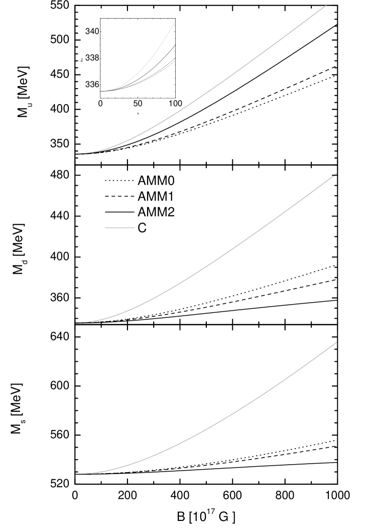
Figure 1: The constituent quark mass as a function of the magnetic intensity at zero baryonic density. Two different regularization schemes, and results with or without AMM are compared as explained in the main text. In the case of the $u$ flavor an insertion shows details for the restricted range $B<10^{19}$ G.

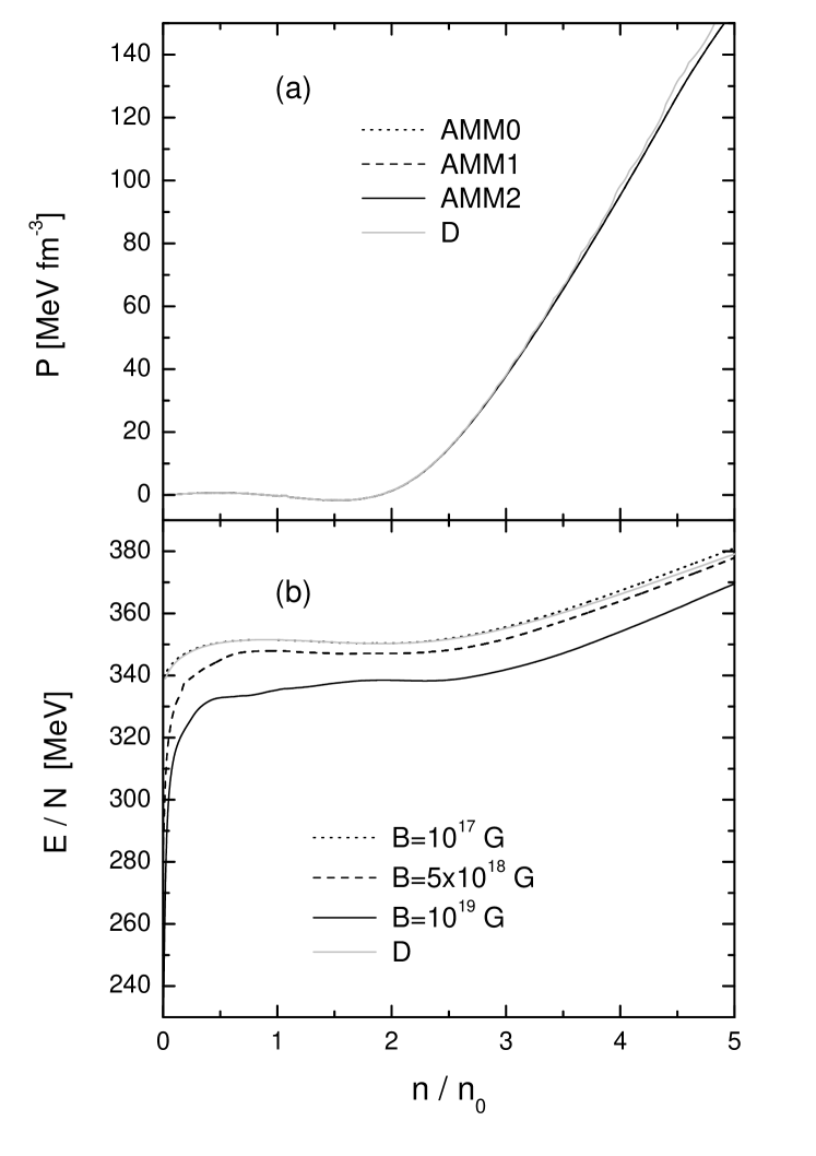
Figure 4: The thermodynamical pressure (a) and the energy per particle (b)as functions of the baryonic density. Results for a model of the variation of the magnetic intensity in the interior of a magnetar (case D) and the results at constant $B=10^{17}$ G with the three set of AMM are included in the first case. In the lower panel the case D is compared with results corresponding to the set AMM1 and different magnetic intensities.

As a first step, different prescriptions for the regularization of the NJL immersed in a uniform magnetic field are considered. A comparison between the present approach and the commonly used procedure as described for instance in EBERT , is made here. In the following the last approach is referred as case C, while the label AMM0 is used for the results of this work when the AMM are zero. In Fig. 1 the constituent quark masses at zero baryonic density are shown as a function of $B$, the wide range of magnetic intensities has the purpose of comparison with previously published works. To appreciate the low intensity behavior a small figure is inserted in the upper panel, restricted to $B<10^{19}$ G. All the approaches agree to predict increasing quark masses, but the rate of growth is always greater in the case C. A comparison between this case and the AMM0 one shows that the difference is accentuated as the magnetic intensity grows, and it is considerable at extreme intensities. However, a regime of qualitative coincidence is found for $B<2\times 10^{18}$ G.
It can be appreciated that the increase of the AMM has opposite effects on the $u$ flavor as compared to the $d,s$ cases. A progressive increase in the magnitude of the AMM enhances the rate of growth for $M_{u}$, while it attenuates the changes in $M_{d},M_{s}$. Due to the smallness of the set AMM1 their results are closer to the AMM0 than to the AMM2.
Calculations of the light quark masses at finite temperature including AMM have been presented in CHAUDHURI . A comparison with these results is risky because they have been obtained in different conditions, i.e. equal particle number of $u$ and $d$ flavors and finite temperature. However, the curves for temperatures below $T=100$ MeV seems to behave similarly. In Fig. 4 of this reference the variation of the quark mass for $B<10^{20}G$ shows quick oscillations around a decreasing mean value when AMM are included, and a slightly decreasing trend is obtained for zero AMM. In contrast, FAYAZ found and almost monotonous increasing trend at zero temperature, and to the greater AMM (set $\kappa_{1}$) corresponds a weaker growth.
The influence of the regularization scheme on the vacuum contribution to the energy density is examined in Fig. 2. In both AMM0 and C approaches a decreasing energy is expected within the range considered here. However in the first case the variation is only of a few MeV, while it exceeds $10$ MeV for intensities slightly above $10^{19}$ G in the last instance.
In conclusion, one can say that there is a qualitative agreement between these procedures in the low magnetic intensity regime, but the discrepancies become important for $B>10^{19}$ G.

In Fig.3 the density dependence of the constituent masses is shown at fixed intensity $B=10^{19}$ G. The figure extends up to baryonic densities $n=7n_{0}$, a density which is feasible in the core of magnetars. The reference value $n_{0}=0.15$ fm^-3 corresponds to the saturation density of nuclear matter. A monotonously decreasing behavior is obtained for all the flavors. In the case of $M_{u}$ there is an almost linear trend at low density till the point $R\approx 1.3$ where the first excited Landau level starts to be occupied. Here a noticeable change of slope takes place. The curve for $M_{s}$ shows a shoulder shape, after a plateau for $3<n/n_{0}<4.5$ a change of slope together with an inflexion point occurs around $n/n_{0}=4.2$. At this density the strange quark comes out to the Fermi sea. The effect of the AMM is almost indistinguishable at the scale shown, but the numerical increments are at most of 10 MeV for the u flavor and around 0.1 MeV for the $s$ quark. The influence of the AMM on the masses of the quarks decreases quickly with the magnetic intensity, so that for $B<5\times 10^{18}$ G all the corrections diminish about 30$\%$.

To take a view of the density effects in the interior of a magnetar a model of the variation of the magnetic field with the density is considered PAL . It is given in terms of the ratio $R=n/n_{0}$ by the formula

$$B(n)=B_{s}+B_{0}\left[1-\exp(-\beta R^{\gamma})\right],$$ (18)

where $B_{s}=10^{15}$ G is the intensity on the star surface, and the remaining parameters have been chosen as $B_{0}=5\times 10^{18}$ G, $\beta=0.01,\;\gamma=3$. The maximum strength $5\times 10^{18}$ G corresponds to asymptotic high densities and could not be reached in a realistic description, hence by the facts just discussed one could expect that the effective quark masses do not manifest the details of the model. For this reason some thermodynamical quantities are examined. The thermodynamical pressure at zero temperature as a function of the baryonic density is exhibited in Fig. 4(a) for a range which covers from the surface to medium depths of a typical neutron star. In the same figure the calculations corresponding to fixed $B=10^{17}$ G and the three sets of the AMM are included. Only small differences are found and at the scale shown all the results seem to coincide. A regime of thermodynamical instability extends for low densities until $R\approx 1.5$ giving rise to the hadronization process. For higher densities $R>3$ the pressure grows almost linearly. The lower panel, Fig. 4(b), is devoted to the energy per particle as a function of the density. In this figure a contrast between the model of density dependent intensity of Eq. (18) (case D)and the results of the set AMM1 at different intensities $B$ is presented. For a given density an increase of the magnetic intensity lessens the energy per particle within the set AMM1. As expected, the outcome of the case D lies between the curves of $10^{17}$ G and $5\times 10^{18}$ G of the parametrization AMM1.

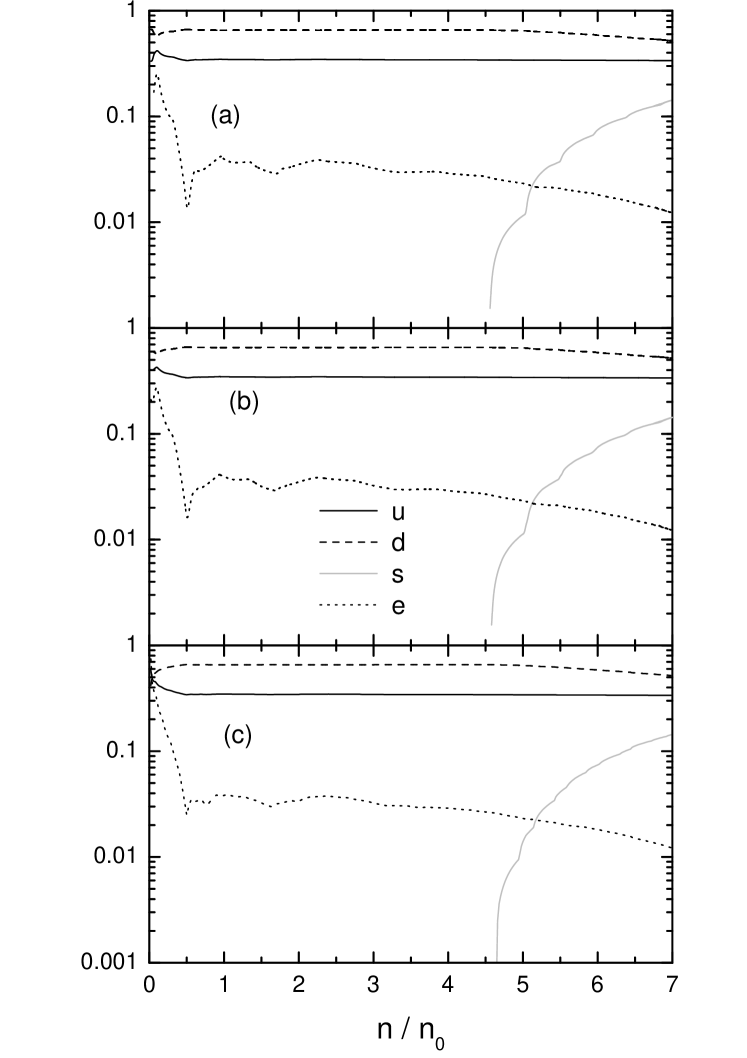
Figure 5: The relative number of particles as a function of the baryonic density for a fixed magnetic intensity $B=5\times 10^{18}$ G. Results corresponding to the AMM0, AMM1 and AMM2 parametrizations are represented in the panel (a), (b) and (c) respectively.

The abundance of particles relative to the total number of quarks is displayed in Fig. 5 as a function of the baryonic density for the fixed intensity $B=5\times 10^{18}$ G. There are no appreciable discrepancies between the different treatments. The inclusion of the AMM produce a slight shift to lower density of the rise of the strange quark population. The population of the strange flavor shows sudden changes of slope, which are noticeable for the sets AMM0 and AMM1, coincident with the occupation of a higher Landau level.

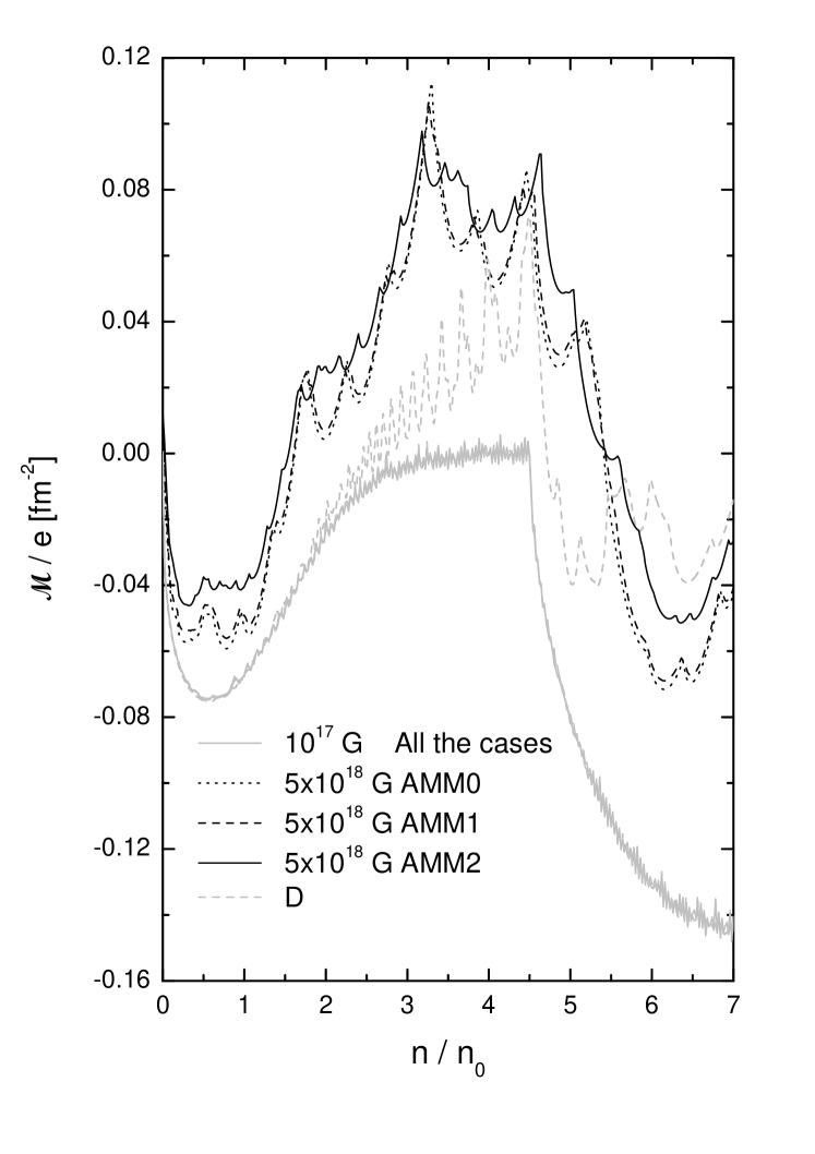
Figure 6: The magnetization as a function of the baryonic density for fixed magnetic intensities $B=10^{17}$ and $B=5\times 10^{18}$ G according to the convention shown. The results for variable intensity of Eq. (18) are also shown (case D).

The magnetization is a measure of the response of the system to the magnetic excitation, it is shown in Fig. 6 as a function of the density. Since this is a very small quantity, the results are scaled with the proton charge, which is appropriate for the range of intensities examined here. In the present case the magnetization receives contributions from the electrons and from the three quark flavors in a proportion determined by the local charge neutrality condition. Different curves corresponding to the constant intensities $B=10^{17}$ G and $B=5\times 10^{18}$ G and the three sets of AMM are displayed. The bottom of this figure is occupied by the lowest intensity results. Because of their similar behavior, the high frequency and the small amplitude of their oscillations, the results of the three parametrizations coalesce into a band. In such conditions the system is essentially diamagnetic for almost all densities. Four different regimes can be clearly distinguished, the limit of zero density with vanishing values of $\cal{M}$ but a steep negative slope. The second one corresponds to low density and extends approximately over the thermodynamic instability region. Here the mean value of the magnetization takes medium values $|{\cal M}/e|<0.08$ fm^-2. For intermediate densities up to the threshold of arising into the Fermi sea of the strange flavor, where the mean of $|{\cal M}/e|$ has their lowest values and remains almost stationary. Finally the high density domain starts with a sudden decrease of the magnetization, which stabilizes asymptotically around the value ${\cal M}/e\approx-0.14$ fm^-2. When the magnetic intensity is increased to $B=5\times 10^{18}$ the pattern just described is kept but other significative differences become apparent. The oscillations have greater amplitudes and do not show a quasi-periodic distribution. This is a manifestation of a coherent dynamics, more favorable at higher intensity due to the smaller number of accessible Landau levels. Furthermore, in the medium density regime the system is definitely paramagnetic while for the higher densities is only moderately diamagnetic. For the model of variable intensity of Eq. (18) the magnetization follows approximately the behavior of the case $B=10^{17}$ G until $R\approx 2$ where it increases abruptly developing quasi periodic oscillations of decreasing frequency and increasing amplitude. In the high density domain it acquires features similar to the case $B=5\times 10^{18}$ G.

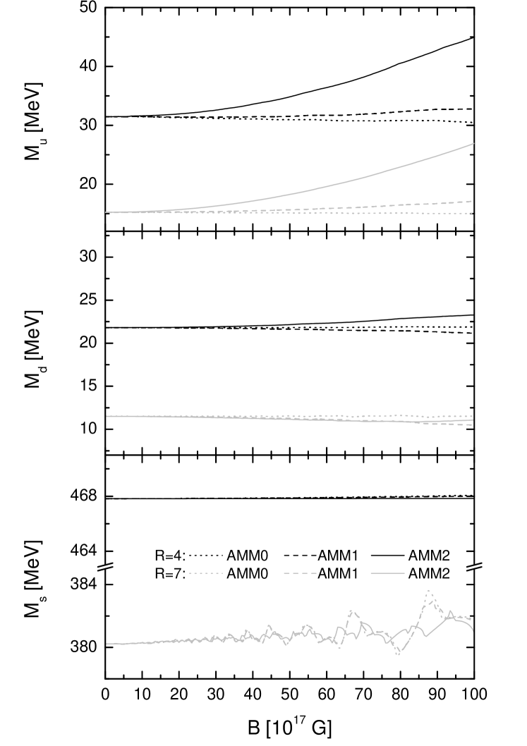
Figure 7: The constituent quark mass as a function of the magnetic intensity for fixed baryonic densities $n/n_{0}=4$ and $7$.

In Fig. 1 the effects of the magnetic intensity on the quark masses in vacuum has been shown. In order to study how the density influence the magnetic dependence, a detail of the results obtained for these masses for non-zero baryonic number is presented in Fig 7. The values chosen for the density, $R=4$ and $R=7$, correspond to situations where quark matter is stable and the s quark is only virtual or is able to exist in the Fermi shell, respectively. A well distinguishable behavior is obtained for the three flavors. The light quarks show a monotonous behavior for the selected densities and the full range of intensities. An increase in the magnitude of the AMM implies an increase for $M_{u}$ independently of the density chosen. Thus the slightly decreasing trend for the set AMM0 becomes moderately increasing for the AMM1 one, and definitely increasing for the AMM2 case. For the $d$ flavor instead, the influence of the AMM is only light at $R=4$ and negligible at $R=7$. For most of the cases it does not have the strength enough to change considerably the almost constant behavior obtained for zero AMM. The mass of the strange quark does not show considerable variations, wherever the values of the AMM. At medium densities $R=4$ it varies monotonously, while for the higher density $R=7$ it exhibits fluctuations whose amplitude increases with B, but do not exceed $2$ MeV.

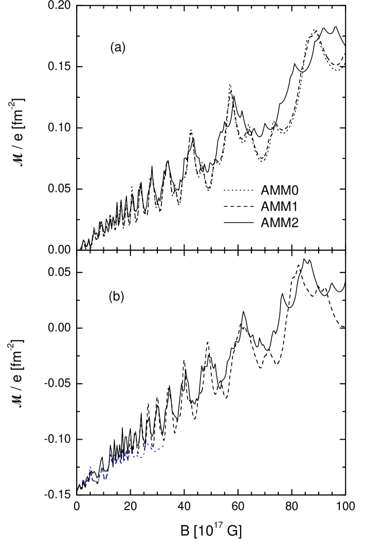
Figure 8: The magnetization as a function of the magnetic intensity for fixed baryonic densities $n/n_{0}=4$ (a), and $n/n_{0}=7$ (b).

Finally, in Fig. 8 the magnetization as a function of the magnetic intensity is shown for the fixed baryonic densities $R=4$ and $R=7$. The typical oscillatory behavior is obtained, whose amplitude as well as mean value increase with $B$. It is interesting to note that for the lower density the system is always paramagnetic, whereas for $n/n_{0}=7$ there is a change of regime and for $B>7.5\times 10^{18}$ G becomes definitely paramagnetic.

IV Summary and Conclusions

In this work a procedure to remove divergences in the $1/N_{c}$ approach to the SU(3) NJL model under a uniform magnetic field $\bm{B}$ has been proposed. The calculations have been made by using a covariant propagator for the quarks with constituent mass, which takes account of the full effect of the magnetic field as well as the effect of the anomalous magnetic moment. There are divergencies which depend on the magnetic intensity. Since the interaction used is an effective model of the strong interaction, a full renormalization is meaningless. Therefore the divergent terms are not ascribed to the renormalization of the external magnetic field since, within the model used, it is not a dynamical variable. In this work a systematic procedure to deal with such kind of divergencies is proposed, instead. To obtain physically meaningful results from the divergent contributions an analytical regularization has been proposed which recovers the standard three momentum cutoff scheme at $B=0$ and arbitrary baryonic density. For this purpose a subtraction of fourth order in the vertices $q_{f}B$ and $\kappa_{f}B$ is performed in the grand potential. Since the regularization point is chosen at $B=0$ and fixed baryonic density, the regularized quantities depend on the quark masses $\tilde{M}_{q}$ evaluated in such conditions. The present approach complements previous work, as for instance EBERT , since it includes $\bm{B}$ dependent terms not considered before as well as the additional coupling of the AMM of the quarks. The regularization scale parameter, typical of the dimensional regularization, has been chosen so as to maximize the agreement with previous studies.

The regularized model has been used to study quark matter in equilibrium against weak decay and electrically neutral, as can be found in the composition of magnetars. A range of magnetic intensities $10^{15}\text{G}\leq B\leq 10^{19}\text{G}$ and baryonic densities $n\leq 1\,\text{fm}^{-3}$ have been analyzed, which are adequate to describe such situation. A model for the magnetic intensity in the interior of a magnetar PAL has been considered to test the results at finite density. For this model the intensity $B$ is parameterized in terms of the baryonic density and ranges between $10^{15}\text{G}\leq B\leq 5\times 10^{18}\text{G}$.

The results at zero baryonic density have been compared with those obtained with the commonly used prescription of EBERT . In general terms a qualitative agreement is obtained for low intensities, but discrepancies become significative for strong magnetic fields $B>5\times 10^{18}$ G. Hence one can conclude that the study of magnetars will probably not evidence completely these differences as in physical situations where the magnetic field manifests with stronger intensity.

A contrast of the results with or without AMM shows that the constituent mass of the $u$ flavor is the more sensitive quantity to these effects, particularly in the medium to high density regime. The magnetization, instead, does not show clear evidence of the influence of the AMM.

Appendix A Regularization of the vacuum contribution to the thermodynamical potential

In this section the Dirac sea contribution to Eq. (8) is regularized, i.e. the contibution coming from the first term of Eq. (6).

In momentum coordinates Eq. (8) can be rewritten as

$$\langle\bar{\psi}_{f}\,i\gamma^{0}\partial_{0}\,\psi_{f}\rangle=-i\;\lim_{\epsilon\rightarrow 0^{+}}\,\int\,\frac{d^{4}p}{(2\pi)^{4}}e^{-i\epsilon p_{0}}p_{0}\text{Tr}\left\{\gamma^{0}\,G_{f}(p)\right\}$$ (19)

Keeping only those terms corresponding to the Dirac sea it reduces to

$$-\frac{2\,i}{(2\pi)^{4}}{\sum_{n,s}}^{\prime}\frac{(-1)^{n}}{\Delta_{n}}\int d^{4}p\,\frac{p_{0}^{2}\;e^{-p_{\bot}^{2}/\beta_{f}}}{u_{p}^{2}-(\Delta_{n}-sK_{f})^{2}+i\varepsilon}\left[\left(\Delta_{n}+s\,M_{f}\right)L_{n}-\left(\Delta_{n}-s\,M_{f}\right)L_{n-1}\right]$$

where the argument of the Laguerre functions $L_{k}$ is $2\,p_{\bot}^{2}/\beta_{f}$ and the primed sum has the same meaning as in the main text.
As usual in analytic regularization, an undetermined scale factor $\nu$ can be introduced RYDER . After a Wick rotation in the $p_{0}p_{z}$ space, the denominator in the previous equation can be rewritten in exponential form by the well known procedure of introducing a new integration on the variable $\tau$ which is well defined in the Euclidean space

$$\frac{2\nu^{-1}}{(2\pi)^{4}}{\sum_{n,s}}^{\prime}\frac{(-1)^{n}}{\Delta_{n}}\int d^{2}p_{\bot}\,d^{2}p_{E}\,p_{4}^{2}\,e^{-p_{\bot}^{2}/\beta_{f}}\left[\left(\Delta_{n}+s\,M_{f}\right)L_{n}-\left(\Delta_{n}-s\,M_{f}\right)L_{n-1}\right]\int_{0}^{\infty}d\tau\,e^{-\tau\left[p_{E}^{2}+(\Delta_{n}-sK_{f})^{2}\right]/\nu}$$

where $d^{2}p_{E}=dp_{4}\,dp_{z}=d\theta dp_{E}p_{E}$ and $p_{4}=p_{E}\cos\theta$. Changing the order, the integration over $d^{2}p_{E}$ can be performed firstly obtaining $\pi\nu^{2}/2\tau^{2}$. As the next step one can integrate over $d^{2}p_{\bot}$ using polar coordinates and with the help of formulae (7.414 6) of G&R . Thus the following expression is obtained

$$\frac{\nu\beta_{f}}{8\pi^{2}}\int_{0}^{\infty}\frac{d\tau}{\tau^{2}}\left[e^{-\tau(M_{f}-K_{f})^{2}/\nu}+\sum_{n=1,s}e^{-\tau(\Delta_{n}-sK_{f})^{2}/\nu}\right] = \frac{\nu\beta_{f}}{8\pi^{2}}\int_{0}^{\infty}\frac{d\tau}{\tau^{2}}\left[\sum_{n=0,s}e^{-\tau(\Delta_{n}-sK_{f})^{2}/\nu}-e^{-\tau(M_{f}+K_{f})^{2}/\nu}\right]$$

$$= \lim_{\epsilon\rightarrow 0}\frac{\nu\beta_{f}}{8\pi^{2}}\int_{0}^{\infty}d\tau\,\tau^{\epsilon-2}\left[\sum_{n,s}e^{-\tau(\Delta_{n}-sK_{f})^{2}/\nu}-e^{-\tau(m+K_{f})^{2}/\nu}\right]$$

In the last line a vanishing parameter $\epsilon$ has been introduced in order to isolate the pole at $\tau=0$. By making a trivial change of integration variable, but different for each term between suare brackets one arrives to

$$\frac{\nu\beta_{f}}{8\pi^{2}}\lim_{\epsilon\rightarrow 0}\left\{\sum_{s,n=0}\left[\frac{(\Delta_{n}-sK_{f})^{2}}{\nu}\right]^{1-\epsilon}-\left[\frac{(m+K_{f})^{2}}{\nu}\right]^{1-\epsilon}\right\}\int_{0}^{\infty}dt\,t^{\epsilon-2}\,e^{-t}$$ (20)

The integral can be identified as $\Gamma(\epsilon-1)$. To put the double summation in a simpler form, and bearing in mind that for $\epsilon=0$ it reduces to

$$\sum_{s,n=0}\frac{(\Delta_{n}-sK_{f})^{2}}{\nu}=\frac{1}{\nu}\sum_{s,n=0}\left(\Delta_{n}^{2}+K_{f}^{2}\right)=\frac{2\beta_{f}}{\nu}\sum_{s,n=0}\left(n+\frac{M_{f}^{2}+K_{f}^{2}}{2\beta_{f}}\right)=\sum_{s}\frac{2\beta_{f}}{\nu}\;\zeta\left(-1,\omega_{f}\right)$$

where the series expansion for the zeta function was used, see for instance Sec. 9.52 of Ref. G&R , and $\omega_{f}=(M_{f}^{2}+K_{f}^{2})/(2\beta_{f})$. Thus, the following approximation is proposed

$$\sum_{s,n=0}\left[\frac{(\Delta_{n}-sK_{f})^{2}}{\nu}\right]^{1-\epsilon}\approx\sum_{s}\;\left(\frac{2\beta_{f}}{\nu}\right)^{1-\epsilon}\zeta\left(\epsilon-1,\omega_{f}\right)$$ (21)

By insering Eq. (21) into Eq. (20) and making a Laurent expansion around $\epsilon=0$ of the resulting expression one obtains

$$-\frac{1}{8\pi^{2}}\lim_{\epsilon\rightarrow 0}\Bigg{\{}\left(\frac{1}{\epsilon}+1-\gamma\right)\left[4\beta_{f}^{2}\zeta\left(-1,\omega_{f}\right)-\beta_{f}\left(M_{f}+K_{f}\right)^{2}\right]+4\beta_{f}^{2}\frac{\partial}{\partial z}\zeta\left(z=-1,\omega_{f}\right)$$

$$-4\beta_{f}^{2}\zeta\left(-1,\omega_{f}\right)\,\ln\left(\frac{2\beta_{f}}{\nu}\right)+\beta_{f}\left(M_{f}+K_{f}\right)^{2}\ln\left(\frac{\left(M_{f}+K_{f}\right)^{2}}{\nu}\right)+{\cal O}(\epsilon)\Bigg{\}}$$ (22)

Here a simple pole is evident, whose residue is a polynomial of fourth order in $B$. As $B\rightarrow 0$ this expression goes as

$$\frac{m^{4}}{8\pi^{2}}\left(\frac{1}{\epsilon}+\frac{3}{2}-\gamma\right)$$ (23)

that is, the typical behavior for a Dirac particle is obtained. The last divergence is usually tackled within this model by the introduction of a constant 3-momentum cutoff $\Lambda$. In this way the following finite contribution is assigned to it

$$\langle\bar{\psi}_{f}\,i\gamma^{0}\partial_{0}\,\psi_{f}\rangle_{NJL}=\frac{N_{c}}{8\pi^{2}}\left[M_{f}^{4}\ln\left(\frac{\Lambda+E_{\Lambda}}{M_{f}}\right)-\Lambda E_{\Lambda}\left(\Lambda^{2}+E_{\Lambda}^{2}\right)\right],$$ (24)

where $E_{\Lambda}=\sqrt{\Lambda^{2}+M_{f}^{2}}$.
In the following we apply to Eq. (22) a procedure that gets rid of the pole term and simultaneously ensures the convergence to Eq. (24) as $B\rightarrow 0$.

In Eq. (22) it can be observed that the magnetic dependence of the residue reduces to order two for $\kappa_{f}=0$, hence the AMM is the cause of new divergencies depending on $B$.
It must be pointed out that this residue satisfies

$$F\left(M,\beta_{f},K\right) = 4\beta_{f}^{2}\zeta\left(-1,\frac{\lambda}{2\beta_{f}}\right)-\beta_{f}\left(M+K\right)^{2}$$ (25)

$$= \left(\sum_{k=0}^{2}\sum_{j=0}^{k}\frac{\beta^{k-j}}{(k-j)!}\frac{K^{j}}{j!}\frac{\partial^{k-j}}{\partial\beta^{k-j}}\frac{\partial^{j}}{\partial K^{j}}+\frac{K^{4}}{4!}\frac{\partial^{4}}{\partial K^{4}}\right)F(M,0,0)$$

Based on this feature the following subtraction procedure is proposed

$$\langle\bar{\psi}_{f}\,i\gamma^{0}\partial_{0}\,\psi_{f}\rangle^{\text{D}}=\langle\bar{\psi}_{f}\,i\gamma^{0}\partial_{0}\,\psi_{f}\rangle_{NJL}+\left[1-\sum_{k=0}^{2}\sum_{j=0}^{k}\frac{\beta_{f}^{k-j}}{(k-j)!}\frac{K_{f}^{j}}{j!}\left(\frac{\partial^{k-j}}{\partial\beta_{f}^{k-j}}\frac{\partial^{j}}{\partial K_{f}^{j}}\right)_{0}-\frac{K^{4}}{4!}\left(\frac{\partial^{4}}{\partial K_{f}^{4}}\right)_{0}\right]\langle\bar{\psi}_{f}\,i\gamma^{0}\partial_{0}\,\psi_{f}\rangle$$ (26)

Where the subindex $0$ means that the derivatives must be evaluated at $\beta_{f}=0,K_{f}=0$. In this way the divergent term cancels out and a finite contribution is generated as $\epsilon\rightarrow 0$. The last one depends on the effective quark masses $\tilde{M}$ evaluated at the regularization point. In the present investigation this point is taken at a fixed baryonic number and zero magnetic intensity. This notation is used to stress that $\tilde{M}$ does not participate of the selfconsistent approach defined by Eq.(1). For the properties of the derivatives of the Hurwitz zeta function, see for instance ELIZALDE .
Thus, the final expression is

$$\langle\bar{\psi}_{f}\,i\gamma^{0}\partial_{0}\,\psi_{f}\rangle^{\text{D}} = \langle\bar{\psi}_{f}\,i\gamma^{0}\partial_{0}\,\psi_{f}\rangle_{NJL}-\frac{N_{c}}{8\pi^{2}}\Bigg{\{}4\beta_{f}^{2}\frac{\partial}{\partial z}\zeta\left(z=-1,\omega_{f}\right)+4\beta_{f}^{2}\zeta\left(-1,\omega_{f}\right)\,\ln\left(\frac{\nu}{2\beta_{f}}\right)-4\beta_{f}^{2}\zeta\left(-1,\tilde{\omega}_{f}\right)\ln\left(\frac{\nu}{\tilde{M}_{f}^{2}}\right)$$ (27)

$$+\beta_{f}\left(M_{f}+K_{f}\right)^{2}\ln\left(\frac{\left(M_{f}+K_{f}\right)^{2}}{\nu}\right)+\frac{\tilde{M}_{f}^{4}}{4}-\frac{K_{f}^{4}}{2}-\frac{\beta_{f}^{2}}{3}-2\beta_{f}K_{f}+\beta_{f}\left(\tilde{M}_{f}+K_{f}\right)^{2}\ln\left(\frac{\nu}{\tilde{M}_{f}^{2}}\right)\Bigg{\}}$$

where $\tilde{\omega}_{f}$ is obtained from $\omega_{f}$ by replacing $M_{f}$ by $\tilde{M}_{f}$
As explained in the main text, if $\nu=M_{f}^{2}$ is adopted the last equation becomes

$$\langle\bar{\psi}_{f}\,i\gamma^{0}\partial_{0}\,\psi_{f}\rangle^{\text{D}} = \langle\bar{\psi}_{f}\,i\gamma^{0}\partial_{0}\,\psi_{f}\rangle_{NJL}-\frac{N_{c}}{8\pi^{2}}\Bigg{\{}4\beta_{f}^{2}\frac{\partial}{\partial z}\zeta\left(z=-1,\omega_{f}\right)+4\beta_{f}^{2}\zeta\left(-1,\omega_{f}\right)\,\ln\left(\frac{M_{f}^{2}}{2\beta_{f}}\right)-8\beta_{f}^{2}\zeta\left(-1,\tilde{\omega}_{f}\right)\ln\left(\frac{M_{f}}{\tilde{M}_{f}}\right)$$ (28)

$$+2\beta_{f}\left(M_{f}+K_{f}\right)^{2}\ln\left(1+\frac{K_{f}}{M_{f}}\right)+\frac{\tilde{M}_{f}^{4}}{4}-\frac{K_{f}^{4}}{2}-\frac{\beta_{f}^{2}}{3}-2\beta_{f}K_{f}+2\beta_{f}\left(\tilde{M}_{f}+K_{f}\right)^{2}\ln\left(\frac{M_{f}}{\tilde{M}_{f}}\right)\Bigg{\}}$$

Using Eqs. (2),(12) and (28) one obtains the regularized thermodynamic potential by taking

$$\langle\bar{\psi}_{f}\,i\gamma^{0}\partial_{0}\,\psi_{f}\rangle=\langle\bar{\psi}_{f}\,i\gamma^{0}\partial_{0}\,\psi_{f}\rangle^{\text{D}}+\langle\bar{\psi}_{f}\,i\gamma^{0}\partial_{0}\,\psi_{f}\rangle^{\text{F}}.$$

Furthermore, the quark condensates are evaluated within the linearized approach KLEVANSKY ; KUNIHIRO ; VOGL ; REHBERG simply as given by Eq. (7)

$$\langle\bar{\psi}_{f}\psi_{f}\rangle=\langle\bar{\psi}_{f}\psi_{f}\rangle^{\text{F}}+\langle\bar{\psi}_{f}\psi_{f}\rangle^{\text{D}}$$

The last term is evaluated by following the same steps as described above. Thus one obtains

$$\langle\bar{\psi}_{f}\psi_{f}\rangle=-\frac{N_{c}}{4\pi^{2}} \Bigg{\{}\left(\frac{1}{\epsilon}+\gamma\right)\left(\beta_{f}K_{f}-\frac{M_{f}^{3}}{2}\right)+2\beta_{f}M_{f}\ln\left(\frac{\Gamma(\omega_{f})}{{\sqrt{2}\pi}}\right)-M_{f}\left(M_{f}^{2}-\beta_{f}\right)\ln\left(\frac{M_{f}^{2}}{2\beta_{f}}\right)$$ (29)

$$+2\beta_{f}\left(M_{f}+K_{f}\right)\ln\left(1+\frac{K_{f}}{M_{f}}\right)+O(\epsilon)\Bigg{\}}$$

To get rid of the divergent term, the following subtraction scheme is performed before taking the limit $\epsilon\rightarrow 0$

$$\langle\bar{\psi}_{f}\psi_{f}\rangle^{\text{D}}=\langle\bar{\psi}_{f}\psi_{f}\rangle_{NJL}+\langle\bar{\psi}_{f}\,\psi_{f}\rangle-\left[1+\beta_{f}K_{f}\frac{\partial^{2}}{\partial\beta_{f}\partial K_{f}}\right]\langle\bar{\psi}_{f}\,\psi_{f}\rangle_{0}$$

where

$$\langle\bar{\psi}_{f}\psi_{f}\rangle_{NJL}=\frac{N_{c}}{2\pi^{2}}M_{f}\left[M_{f}^{2}\ln\left(\frac{\Lambda+E_{\Lambda}}{M_{f}}\right)-\Lambda E_{\Lambda}\right]$$

The following result is obtained finally

$$\langle\bar{\psi}_{f}\psi_{f}\rangle^{\text{D}}=\langle\bar{\psi}_{f}\psi_{f}\rangle_{NJL}-\frac{N_{c}}{4\pi^{2}} \Bigg{\{}2\beta_{f}M_{f}\ln\left(\frac{\Gamma(\omega_{f})}{{\sqrt{2}\pi}}\right)-M_{f}\left(M_{f}^{2}-\beta_{f}\right)\ln\left(\frac{M_{f}^{2}}{2\beta_{f}}\right)$$ (30)

$$+2\beta_{f}\left(M_{f}+K_{f}\right)\ln\left(1+\frac{K_{f}}{M_{f}}\right)+\tilde{M}_{f}^{3}\Bigg{\}}$$

Figure 2: The energy density (with changed sign) at zero chemical potential as a function of the magnetic intensity for different regularization schemes.

Figure 3: The constituent quark mass as a function of the baryonic density for a fixed magnetic intensity $B=10^{19}$ G.

References

- (1) V. A. Miransky, and I. A. Shovkovy, Phys. Rept. 576 (2015), and references therein.
- (2) J. O. Andersen, W. R. Naylor, A. Tranberg, Rev. Mod. Phys. 88 (2016) 025001, and references therein.
-
(3)
S.P. Klevansky, R. H. Lemmer, Phys.Rev. D 39 (1989) 3478,
S. P. Klevansky, Rev. Mod. Phys. 64 (1992) 649. - (4) V. P. Gusynin, V.A. Miransky, I.A. Shovkovy, Phys.Lett. B 349 (1995) 477-483
- (5) D. Ebert, K. G. Klimenko, M. A. Vdovichenko, and A. S. Vshivtsev, Phys. Rev. D 61 (1999) 025005.
- (6) E. J. Ferrer, V. de la Incera, C. Manuel, Nucl.Phys. B 747 (2006) 88-112.
- (7) J. L. Noronha, I. A. Shovkovy, Phys.Rev. D 76 (2007) 105030.
- (8) I.E. Frolov, V.Ch. Zhukovsky, K.G. Klimenko, Phys.Rev. D 82 (2010) 076002.
- (9) B. Chatterjee, H. Mishra, A. Mishra, Phys.Rev. D 84 (2011) 014016.
- (10) R. Z. Denke, M. B. Pinto, Phys.Rev. D 88 (2013) 056008.
- (11) E. J. Ferrer, V. de la Incera, I. Portillo, M. Quiroz, Phys.Rev. D 89 (2014) 085034.
- (12) A. Abhishek, H. Mishra, Phys.Rev. D 99 (2019) 054016.
- (13) H. Pais, D. P. Menezes, C. Providencia, Phys.Rev. C 93 (2016) 065805.
- (14) S. K. Blau, M. Visser, A. Wipf, Int. J. Mod. Phys. A 6 (1991) 5409.
- (15) A. Goyal, M. Dahiya, Phys.Rev. D 62 (2000) 025022.
- (16) T. D. Cohen, E. S. Werbos, Phys.Rev. C 80 (2009) 015203.
- (17) M. Ruggieri, M. Tachibana, Vincenzo Greco, JHEP 1307 (2013) 165.
- (18) J. O. Andersen, R. Khan, Phys.Rev. D 85 (2012) 065026.
- (19) D.P. Menezes, M. Benghi Pinto, S.S. Avancini, A. Perez Martinez, C. Providencia, Phys.Rev. C 79 (2009) 035807.
- (20) Sh. Fayazbakhsh, S. Sadeghian, N. Sadooghi, Phys.Rev. D 86 (2012) 085042.
- (21) A. Amador, J. O. Andersen, Phys.Rev. D 88 (2013) 025016.
- (22) S. S. Avancini, V. Dexheimer, R. L. S. Farias, V. S. Timoteo, Phys. Rev. C 97 (2018) 035207.
- (23) S. S. Avancini, R. L. S. Farias, and W. R. Tavares, Phys. Rev. D 99 (2019) 056009.
- (24) S. S. Avancini, R. L.S. Farias, N. N. Scoccola, W. R. Tavares, Phys.Rev. D 99 (2019) 116002.
- (25) Sh. Fayazbakhsh, N. Sadooghi, Phys.Rev. D 90 (2014) 105030.
- (26) N. Chaudhuri, S. Ghosh, S. Sarkar, and P. Roy, Phys. Rev. D 99 (2019) 116025.
- (27) J. P. Singh, Phys.Rev. D 31 (1985) 1097.
- (28) Pedro J. de A. Bicudo, J. E. Ribeiro, R. Fernandes, Phys. Rev. C 59 (1999) 1107.
- (29) Mustapha Mekhfi, Phys.Rev. D 72 (2005) 114014.
- (30) R. G. Felipe, A. Perez Martinez, H. Perez Rojas, M. Orsaria, Phys.Rev. C 77 (2008) 015807.
- (31) R. M. Aguirre, A. L. De Paoli, Eur. Phys. J. A 52 (2016) 343.
- (32) R. M. Aguirre, Phys. Rev. D 95 (2017) 074029
- (33) R.M. Aguirre, Phys. Rev. D 96 (2017) 096013; R. M. Aguirre, Eur. Phys. J. A 55 (2019) 28.
- (34) T. Hatsuda, T. Kunihiro, Phys.Rept. 247 (1994) 221.
- (35) U. Vogl, W. Weise, Prog. Part. Nucl. Phys. 27 (1991) 195.
- (36) N.P. Landsman, C.G. van Weert, Phys. Rept. 145 (1987) 141.
- (37) M. Buballa, Phys.Rept. 407 (2005) 205.
- (38) A. Broderick, M. Prakash, and J. M. Lattimer, Astroph. J. 537 (2000) 351.
- (39) D. Bandyopadhyay, S. Chakrabarty, S. Pal, Phys. Rev. Lett. 79 (1997) 2176.
- (40) L. H. Ryder, Quantum Field Theory, 2nd edition Cambridge University Press, 1996.
- (41) I. S. Gradshteyn, I. M. Ryzhik, Tables of integrals, series and products, 7th edition, Academic Press, 2007.
- (42) E. Elizalde, S. D. Odintsov, A. Romeo, A. A. Bytsenko, S. Zerbini, Zeta regularization techniques with applications, World Scientific Publishing, 1994.
- (43) P. Rehberg, S. P. Klevansky, J. Hufner, Phys. Rev. C 53 (1996) 410.