Gapless quantum spin liquid and global phase diagram of the spin-1/2 $J_{1}$-$J_{2}$ square antiferromagnetic Heisenberg model

Abstract

The nature of the zero-temperature phase diagram of the spin-$1/2$ $J_{1}$-$J_{2}$ Heisenberg model on a square lattice has been debated in the past three decades, which may hold the key to understand high temperature superconductivity. By using the state-of-the-art tensor network method, specifically, the finite projected entangled pair state (PEPS) algorithm, to simulate the global phase diagram the $J_{1}$-$J_{2}$ Heisenberg model up to $24\times 24$ sites, we provide very solid evidences to show that the nature of the intermediate nonmagnetic phase is a gapless quantum spin liquid (QSL), whose spin-spin and dimer-dimer correlations both decay with a power law behavior. There also exists a valence-bond solid (VBS) phase in a very narrow region $0.56\lesssim J_{2}/J_{1}\leq 0.61$ before the system enters the well known collinear antiferromagnetic phase. The physical nature of the discovered gapless QSL and potential experimental implications are also addressed. We stress that we make the first detailed comparison between the results of PEPS and the well-established density matrix renormalization group (DMRG) method through one-to-one direct benchmark for small system sizes, and thus give rise to a very solid PEPS calculation beyond DMRG. Our numerical evidences explicitly demonstrate the huge power of PEPS for precisely capturing long-range physcis for highly frustrated systems, and also demonstrate the finite PEPS method is a very powerful approach to study strongly corrleated quantum many-body problems.

I Introduction

Since the discovery of high-Tc cuprates, people conjectured that a spin-$1/2$ antiferromagnetic Heisenberg model on square lattice with nearest neighbor (NN) couplings $J_{1}$ and next nearest neighbor (NNN) couplings $J_{2}$ (known as the square lattice $J_{1}$-$J_{2}$ model) would support a quantum spin liquid (QSL) phase, which could serve as the primary low-energy metastable states before the systems enter the superconducting phase Anderson (1987); Wen et al. (1989); Read and Sachdev (1991); Lee et al. (2006); Poilblanc et al. (2014). The Hamiltonian of this model reads:

$$H=J_{1}\sum_{\langle i,j\rangle}\mathbf{S_{i}}\cdot\mathbf{S_{j}}+J_{2}\sum_{\langle\langle i,j\rangle\rangle}\mathbf{S_{i}}\cdot\mathbf{S_{j}},\quad(J_{1},J_{2}>0),$$ (1)

For the intermediate $J_{2}$ coupling regime, it is long believed that the quantum fluctuation will destroy the antiferromagnetic (AFM) long range order before the maximally frustrated point $J_{2}/J_{1}=0.5$ of the classical model and might establish a new paramagnetic phase. The nature of such a paramagnetic phase is of great interest and it might hold the key mechanism of high-Tc cuprates. In early days of high-Tc research, the square lattice $J_{1}$-$J_{2}$ model was thus one of the most important frustrated magnet models, and attracted intense research interest, both theoretically and experimentally. In past three decades tremendous efforts by different kinds of methods have been developed to investigate the intermediate paramagnetic phase Chandra and Doucot (1988); Dagotto and Moreo (1989); Figueirido et al. (1990); Sachdev and Bhatt (1990); Poilblanc et al. (1991); Chubukov and Jolicoeur (1991); Schulz and Ziman (1992); Ivanov and Ivanov (1992); Einarsson and Schulz (1995); H. J. Schulz and Poilblanc (1996); Zhitomirsky and Ueda (1996); Singh et al. (1999); Capriotti and Sorella (2000); Capriotti et al. (2001); Zhang et al. (2003); Takano et al. (2003); Sirker et al. (2006); Schmalfuß et al. (2006); Mambrini et al. (2006); Darradi et al. (2008); Arlego and Brenig (2008); Isaev et al. (2009); Murg et al. (2009); Beach (2009); Richter and Schulenburg (2010); Yu and Kao (2012); Jiang et al. (2012); Mezzacapo (2012); Wang et al. (2013); Hu et al. (2013); Doretto (2014); Qi and Gu (2014); Gong et al. (2014); Chou and Chen (2014); Morita et al. (2015); Richter et al. (2015); Wang et al. (2016); Poilblanc and Mambrini (2017); Wang and Sandvik (2018); Haghshenas and Sheng (2018); Liu et al. (2018); Poilblanc et al. (2019), and different candidate ground states were proposed, including a columnar valence-bond solid (CVBS) state Dagotto and Moreo (1989); Poilblanc et al. (1991); Schulz and Ziman (1992); Sachdev and Bhatt (1990); Chubukov and Jolicoeur (1991); Singh et al. (1999); Haghshenas and Sheng (2018), a plaquette valence-bond solid (PVBS) state Zhitomirsky and Ueda (1996); Capriotti and Sorella (2000); Takano et al. (2003); Mambrini et al. (2006); Darradi et al. (2008); Arlego and Brenig (2008); Isaev et al. (2009); Yu and Kao (2012); Doretto (2014); Gong et al. (2014); Morita et al. (2015); Wang and Sandvik (2018); Ferrari and Becca (2020); Nomura and Imada (2021), and a gapless QSL state Capriotti et al. (2001); Zhang et al. (2003); Wang et al. (2013); Hu et al. (2013); Qi and Gu (2014); Richter et al. (2015); Poilblanc and Mambrini (2017); Liu et al. (2018); Morita et al. (2015); Wang and Sandvik (2018); Ferrari and Becca (2020); Nomura and Imada (2021), as well as a gapped QSL state Jiang et al. (2012). Unfortunately, the physical nature of the paramagnetic phase is still enigmatic.

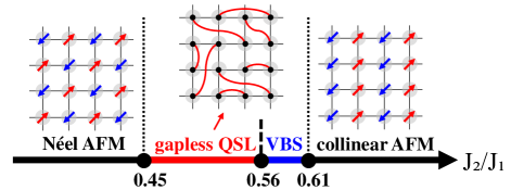
Figure 1: The phase diagram of spin-1/2 $J_{1}$-$J_{2}$ square-lattice Heisenberg antiferromagnetic model. The nonmagnetic region is $0.45\lesssim J_{2}\leq 0.61$, and it is a gapless spin liquid phase for $0.45\lesssim J_{2}\lesssim 0.56$ and a VBS phase for $0.56\lesssim J_{2}\leq 0.61$.

To understand the properties of potential QSL phase of frustrated magnets systematically, X.-G. Wen created the framework of the projective symmetry group (PSG) Wen (1991) and proposed many different types of QSL variational states for the square lattice $J_{1}$-$J_{2}$ model. Among different variational quantum Monte Carlo (vQMC) calculations Capriotti et al. (2001); Hu et al. (2013); Chou and Chen (2014); Morita et al. (2015), a particular gapless $Z_{2}$ QSL state was intensively studied with Lanczos projection Hu et al. (2013). As its variational energy is the lowest one among all possible QSL constructed by projective wavefunctions classified by PSG, and is also competitive with the most accurate DMRG ones, people conjecture that such a QSL state could be stabilized in the intermediate paramagnetic phase. However, it is still unclear whether a second order phase transition is possible between such a QSL phase and the usual Néel AFM phase. Morevoer, the PSG framework only considers symmetry fractionalization patterns for spinons and, hence, cannot capture all gapped QSL phases predicted by the general theoretical concept of symmetry enriched topological (SET) order Barkeshli et al. (2019). Thus, it would not be a surprise if the PSG framework cannot describe all gapless QSL states as well.

On the other hand, as there are also numerical evidences indicating that a valence-bond solid (VBS) Dagotto and Moreo (1989); Poilblanc et al. (1991); Schulz and Ziman (1992); Sachdev and Bhatt (1990); Chubukov and Jolicoeur (1991); Zhitomirsky and Ueda (1996); Singh et al. (1999); Haghshenas and Sheng (2018); Capriotti and Sorella (2000); Takano et al. (2003); Mambrini et al. (2006); Darradi et al. (2008); Arlego and Brenig (2008); Isaev et al. (2009); Yu and Kao (2012); Doretto (2014); Gong et al. (2014) might develop in the intermediate paramagnetic phase, an alternative scenario —- the deconfined quantum critical point (DQCP) Senthil et al. (2004a, b); Sirker et al. (2006); Sandvik (2007, 2010a); Nahum et al. (2015); Shao et al. (2016); Lou et al. (2009); Sandvik and Zhao (2020) was also proposed to describe the direct phase transition between the usual Néel AFM phase and the VBS phase. DQCP is an intrinsically strong coupling quantum critical point and it is indeed a Landau forbidden second order phase transition between two ordered phases. This kind of phase transition has already been observed in frustrated-free models, e.g., the $J$-$Q$ model first proposed by Anders Sandvik Sandvik (2007).

For convenience, we set $J_{1}=1$ throughout the whole paper. An early density matrix renormalization group (DMRG) study suggests that the nonmagnetic region $0.41\lesssim J_{2}\lesssim 0.62$ is a gapped ${\rm Z_{2}}$ spin liquid phase Jiang et al. (2012), without any spin and dimer orders in the thermodynamic limit. However, a more recent DMRG study with SU(2) symmetry proposes a PVBS phase for $0.5\lesssim J_{2}\lesssim 0.61$ with a near critical region $0.44\lesssim J_{2}\lesssim 0.5$ Gong et al. (2014). Later, a very recent DMRG study further proposes two phases in the nonmagnetic region: a gapless spin liquid phase for $0.46\lesssim J_{2}\lesssim 0.52$ and a VBS phase for $0.52\lesssim J_{2}\lesssim 0.62$ Wang and Sandvik (2018). On the other hand, a vQMC study Hu et al. (2013) and a finite projected entangled pair state (PEPS) Liu et al. (2018) suggest a gapless QSL phase in the entire intermediate nonmagnetic region. A well known fact is that DMRG is almost numerically exact, but essentially as a one-dimensional algorithm, the precision of DMRG for 2D systems strongly depends on the system width and states kept. New approaches that can go beyond DMRG for 2D simulation is in great ungency. PEPS, a higher dimensional extension of DMRG, which is also a systemtically improvable variational ansatz, provides a very promising tool for solving 2D quantum many-body problems Verstraete and Cirac (2004); Verstraete et al. (2006, 2008). However, the expensive cost of PEPS greatly limits its practical application. Recently, in the scheme of combining variational Monte Carlo method and tensor network states Sandvik and Vidal (2007); Schuch et al. (2008); Sandvik (2008); Wang et al. (2011); Liu et al. (2017), where physical quantities can be evaluated through Monte Carlo sampling and ground states can be obtained by the means of gradient optimization, an accurate PEPS method was established to deal with finite 2D systems on open boundary conditions (OBC) Liu et al. (2021a), making it possible to simulate large systems with very high precision. Particularly, it allows us to compare PEPS and DMRG results directly on the same system, which could be crucial to clarify some long-standing controversial many-body problems.

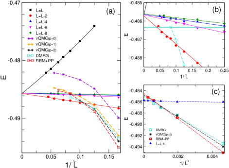
Figure 2: (a) Comparison of ground state energies in the thermodynamic limit at $J_{2}/J_{1}=0.55$. Different central bulk choices $\tilde{L}\times\tilde{L}$ are used for extrapolations of the $D=8$ optimized PEPS energies. The solid lines denotes a second order polynomial fit for $\tilde{L}=L$ or a linear fit for the other cases, with extrapolated values lying in a small window about $[-0.4857,-0.4856]$. The vQMC energies with PBC, RBM+PP energies with PBC, and DMRG energies with CBC are presented, taken from Ref. Hu et al. (2013), Ref. Nomura and Imada (2021) and Ref. Gong et al. (2014), respectively. (b) A detailed scale comparison of finite-size effects between PEPS and DMRG, sharing the same legends with (a). The solid cyan line denotes DMRG energy $-0.4863$ on a cylinder with circumference $L=12$ lattice spacings. (c) Dashed lines denote fits using $E(\tilde{L})=E_{\infty}+c/\tilde{L}^{3}$. Energies of $\tilde{L}=L=6-12$ for DMRG  Gong et al. (2014), $\tilde{L}=L=6-10$ for vQMC (p=2) Hu et al. (2013), and $\tilde{L}=L=6-16$ for RBM+PP Nomura and Imada (2021) are used to fit. PEPS energies using $\tilde{L}=L-4$ (blue triangle) are shown for comparison with an extrapolated value $E_{\infty}=-0.48580(4)$ and a coefficient $c=0.061(19)$ via such a linear fit of $1/\tilde{L}^{3}$.

In this paper, we apply the state-of-the-art finite PEPS method to accurately simulate the $J_{1}$-$J_{2}$ model up to $24\times 24$. Our results show that the nonmagnetic region $0.45\lesssim J_{2}\leq 0.61$ consists of a gapless QSL phase for $0.45\lesssim J_{2}\lesssim 0.56$ and a VBS phase for $0.56\lesssim J_{2}\leq 0.61$. The QSL phase is gapless by observing a power law decay of both spin-spin and dimer-dimer correlation functions. Through detailed comparison with DMRG, we provide very solid numerical results beyond DMRG. We also propose an effective field theory to understand the nature of such a gapless spin liquid and discuss the potential relationship with DQCP scenario.

The rest of the paper is organized as follows. In Sec.II, we show the energy comparison with other methods, and present the global phase diagram including critical exponents by measuring order parameters. In Sec.III, we compare spin-spin correlations with DMRG calculations and analyze their decay behavior in details. We also analyze the decay behavior of dimer-dimer correlations. In Sec. IV we discuss the nature of the paramagnetic region and interpret the quantum phase transitions with quantum field theories. In Sec. V we discuss our results and explain the origin of different scenarios from other studies.

II Global phase diagram

II.1 Finite-size scaling of ground state energy.

We begin with the computation of ground state energies. All energies and order parameters are computed with $D=8$ PEPS, if not otherwise specified. We first compare PEPS ground state energies with available DMRG energies and variational QMC energies. Although our systems are based on open boundaries, finite-size scaling (FSS) formulas can still work very well Liu et al. (2021a). In a previous work, it has been shown that our method has extremely high precision for both unfrustated and frustrated models Liu et al. (2021a). For the unfrustrated case, i.e., $J_{2}=0$, the obtained energies and magnetizations agree excellently with standard (QMC) results. For frustrated cases, the ground state energy in 2D limit at $J_{2}=0.5$ is $-0.49635(5)$, very close to the corresponding DMRG lower bound energy with $-0.4968$. Here we check the ground state energy at another highly frustrated point $J_{2}=0.55$. We compute systems $L\times L$ for $L=8-24$. Shown in Fig. 2(a), we use the whole system $\tilde{L}=L$ for FSS versus $1/\tilde{L}$ to obtain the extrapolated energy with $-0.48572(9)$. Alternatively, we can also use other central bulk choices such as $\tilde{L}=L-2$, $\tilde{L}=L-4$ for FSS, and they give almost the same extrapolated energies. The DMRG energies with cylindrical boundary condition (CBC) taken from Ref. Gong et al. (2014), and the vQMC energies with different Lanczos projection steps with periodic boundary condition (PBC) taken from Ref. Hu et al. (2013) and are also presented, as well as the PBC energies from a method combining restricted Boltzmann machine and pair-product states (RBM+PP) Nomura and Imada (2021). The DMRG and vQMC p=2 energies on each size look very close, while this might be a coincidence. In Fig. 2(b), we note that the estimated 2D limit DMRG energy $E_{\rm DMRG}\simeq-0.4863$ should be regarded as their lower bound due to finite-size effects. The extrapolated 2D limit energy of PEPS from finite size scaling is about $-0.48572(9)$, very close to the DMRG lower bound energy $-0.4863$. These results are are from different boundary conditions, and we can use their obtained extrapolated energy in the 2D limit for indirect comparison. For frustrated models with CBC and PBC, the precise energy leading scaling with respect to linear system size $L$ is theoretically unclear. Considering CBC and PBC have small boundary effects, usually people can reasonably assume the energy scales as $E(\tilde{L})=E_{\infty}+c/\tilde{L}^{3}$ where $\tilde{L}=L$ for DMRG, vQMC and RBM+PP results, according to the knowledge on the Heisenberg model Stoudenmire and White (2012). Such a $1/L^{3}$ leading scaling indeed seems to work well for fittings, and the obtained 2D energy of DMRG results using $L=6-12$ Gong et al. (2014), vQMC p=2 results using $L=6-10$ Hu et al. (2013) and RBM+PP results using $L=6-16$ Nomura and Imada (2021) are $-0.4852(2)$, $-0.4848(3)$ and $-0.4845(1)$, respectively, shown in Fig. 2(c). If $L=6$ is excluded, the fits (not shown in Fig. 2(c) for clearness) give corresponding DMRG, vQMC p=2 and RBM+PP extrapolated energy about $-0.48552(7)$, $-0.4854$ (only two points for fit) and $-0.4846(1)$, still higher than our obtained 2D energy $-0.48572(9)$. In anyway, these detailed analyses demonstrate our energy is among the most accurate ones. A similar analysis at $J_{2}=0.5$ can be found in Appendix. B. We would mention that because our finite PEPS energies are based on open boundary conditions, due to boundary effects, one should neither directly compare them with DMRG or vQMC results size by size, nor use the large size energy, say $24\times 24$, as an 2D estimation to directly compare with other 2D estimated energies. Nevertheless, the central bulk energy like $\tilde{L}=L-4$ show much smaller finite-size effects and can be used to directly estimate the 2D limit energy, as is seen in Fig. 2(a) and (c).

II.2 Finite-size scaling of order parameters and critical exponents

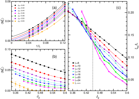
Figure 3: (a) The Néel AFM order $\langle{\bf M}_{0}^{2}\rangle$ of the $D=8$ optimized PEPS on $L\times L$ lattices up to $L=24$. Finite-size extrapolations through a second order polynomial fit. (b) The $J_{2}$ dependence of $\langle{\bf M}_{0}^{2}\rangle$ on different systems from $L=8$ to 24. The 2D limit estimated values are also shown as orange sysmbols. (c) The scaling of crossing points of the dimensionless quantity $\xi_{m}/L$ used to extract critical point $J_{c1}$ at different $J_{2}$ from $L=8$ to 24.

Now we consider spin orders including AFM Néel order and collinear order. The spin order parameter (squared) is expressed as $m^{2}_{s}({\bf k})=\frac{1}{L^{4}}\sum_{\bf{ij}}\langle{\bf S}_{{\bf i}}\cdot{\bf S}_{{\bf j}}\rangle{e}^{i{\bf k}\cdot({\bf i}-{\bf j})}$, where ${\bf i}=(i_{x},i_{y})$ is the site position. The Néel order parameter (squared) corresponds to the value at $\bf k_{0}=(\pi,\pi)$, i.e., $m^{2}_{s}({\bf k_{0}})=\langle{\bf M}_{0}^{2}\rangle$, where

$${\bf M}_{0}=\frac{1}{L^{2}}\sum_{\bf i}(-1)^{\bf i}{\bf S}_{{\bf i}}\,.$$ (2)

In Fig. 3(b), we present the AFM Néel order on different $L\times L$ systems up to $24\times 24$. Our results suggest that the Néel order vanishes around $J_{c1}=0.45$ in the thermodynamic limit via FSS. Note that, for $J_{2}\geq 0.45$, a power law fit, instead of polynomial one, is more relevant (see Appendix B). Alternatively, we also use a dimensionless quantity $\xi_{m}/L$ to evaluate the critical point where $\xi_{m}$ is a correlation length defined as $\xi_{m}=\frac{L}{2\pi}\sqrt{\frac{m^{2}_{s}(\pi,\pi)}{m^{2}_{s}(\pi,\pi+2\pi/L)}-1}$ Sandvik (2010b). From the results of $L=16$, 20 and 24 in Fig. 3(c), we can see the critical point is indeed located at $J_{c1}\simeq 0.45$, well consistent with the above result. We also find that the collinear AFM order appears at $J_{c3}=0.61$ via a first order transition, and we will discuss more details for $J_{c3}$ in the Appendix. C.

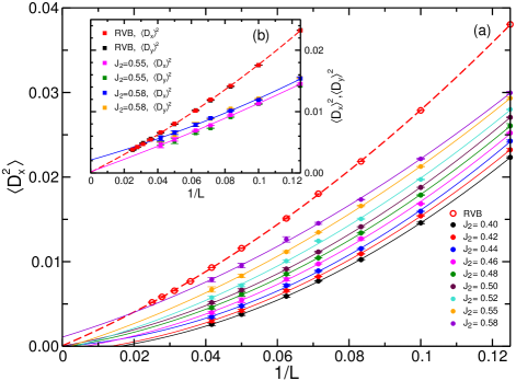
Figure 4: Finite-size scaling of the VBS order parameter of the $D=8$ optimized PEPS. Results for the RVB state on finite systems are used as references. (a) VBS order parameter based on bond-bond correlations. (b) Local VBS order induced by boundaries. All extrapolations are performed through a second-order polynomial fitting.

Next we measure the dimer order parameters to detect the possibility of VBS order in the nonmagnetic region $0.45\lesssim J_{2}\leq 0.61$. The bond operator is defined as $B^{\alpha}_{\bf i}={\bf S}_{{\bf i}}\cdot{\bf S}_{{\bf i}+{\rm e_{\alpha}}}$ between site ${\bf i}$ and site ${\bf i}+{\rm e_{\alpha}}$ along $\alpha$ direction with $\alpha=x$ or $y$. Then we can use the dimer order parameter (DOP)

$$D_{\alpha}=\frac{1}{N_{b}}\sum_{{\bf i}}(-1)^{i_{\alpha}}B^{\alpha}_{\bf i}$$ (3)

to detect possible VBS patterns Zhao et al. (2020), where $N_{b}=L(L-1)$ is the total number of counted bonds. For spin liquid states, $\langle D^{2}_{\alpha}\rangle$ and $\langle D_{\alpha}\rangle^{2}$ should be zero in the thermodynamic limit. In Fig. 4(a), we present the horizontal dimer orders $\langle D^{2}_{x}\rangle$ for $J_{2}$ ranging from 0.40 to 0.58. By extrapolation to 2D limit, we find that the dimer values are zero for $J_{2}\leq$ 0.55, while there is a small nonzero value for $J_{2}=0.58$, indicating a potential weak VBS phase. For further analysis, we compare the $J_{1}$-$J_{2}$ results with a resonant valence bond (RVB) state, which is a gapless spin liquid described by a $D=3$ PEPS Wang et al. (2013). The dimer orders of such a RVB state are accurately computed on open boundary conditions up to $40\times 40$ sites. Typically, the dimer values of $\langle D^{2}_{x}\rangle$ of $J_{1}$-$J_{2}$ model are smaller than those of the RVB state. For comparison, we consider the finite-size scaling behavior $\langle D^{2}_{x}\rangle\sim L^{-(1+\eta^{\prime}_{d})}$ which is expected to be more relevant than the polynomial fit of Fig. 4(a) when $\langle D_{\alpha}\rangle=0$ (see Appendix B). With increasing $J_{2}$ from 0.40 to 0.55, $\eta^{\prime}_{d}$ will decrease from 0.96(2) to 0.32(2), but all of them are larger than those of the RVB state with $\eta^{\prime}_{d}=0.23(1)$, indicating the corresponding extrapolated dimer values must be zero. However, for $J_{2}=0.58$, $\eta^{\prime}_{d}=0.18(2)$, which is slightly smaller than the RVB state.

We further directly check the dimer values $\langle D_{\alpha}\rangle^{2}$ which are induced by the boundaries, shown in Fig. 4(b). In general, we find $\langle D_{x}\rangle^{2}$ is almost the same as $\langle D_{y}\rangle^{2}$, showing a good isotropic behavior between the $x-$ and $y-$ directions. For $J_{2}=0.55$, the induced dimerizations $\langle D_{\alpha}\rangle^{2}$ are also zero in the thermodynamic limit, while for $J_{2}=0.58$ the extrapolated value $\langle D_{\alpha}\rangle^{2}\simeq 0.0026(11)$ is finite, consistent with $\langle D_{\alpha}^{2}\rangle\simeq 0.0018(9)$ and, hence, with a VBS phase at $J_{2}=0.58$. In addition, to further check the extrapolated value $\langle D^{2}_{x}\rangle$ at $J_{2}=0.58$, we also try second order fittings with different fitting intervals. The extrapolated values by using 4 large-L data, 5 large-L data and 6 large-L data to fit , are $-0.0007(31)$, $-0.0009(23)$ and 0.0025(11), respectively. Note for the 4 large-L data and 5 large-L data fits, the extrapolated values have a large uncertainty, which is probably due to the lack of data to fit. A third order fitting function for the all available points gives 0.0031(12), consistent with the second-order fitted value 0.0018(9). These extrapolated values are compatible with the induced dimerization $\langle D_{\alpha}\rangle^{2}\simeq 0.0026(11)$. Actually, the VBS is further supported by the decay behaviours of correlation functions, which we will discuss in next section. In summary, our results suggest that in the nonmagnetic region $0.45\lesssim J_{2}\leq 0.61$, a spin liquid phase covers a large region, and there is also a small window for a weak VBS phase around $J_{2}=0.58$.

In order to extract critical exponents, we further analyse the scaling of obtained quantities. As mentioned above, the AFM-QSL transition point can be precisely located by the crossing of the dimensionless quantity $\xi_{m}/L$ at $J_{c1}=0.45(1)$ which has relatively small finite size effects Sandvik (2010b). In fact, such an approach is equivalent to the so-called correlation ratio method Kaul (2015); Nomura and Imada (2021), both using the value of $m^{2}_{s}(\pi,\pi)/m^{2}_{s}(\pi,\pi+2\pi/L)$. In terms of $\xi_{m}/L$, it can be further used to extract the correlation length exponent $\nu$ Sandvik (2010b). For the QSL-VBS transition, in principle similar correlation length from dimer structure factor information can be also applied to locate the transition point. Unfortunately, the dimer structure factor is not well defined on open boundary conditions Zhao et al. (2020). Nevertheless, the QSL-VBS transition point can still be located at $J_{c1}=0.56(1)$, according to the finite size scaling of order parameters, as well as the spin-spin correlation decay behaviours which is shown in next part. Now we extract the correlation length exponents $\nu$ by scaling $\xi_{m}$ at the AFM-QSL transition point. To obtain a good data collpase, we use the scaling formula with a subleading correction Sandvik (2007):

$$\xi_{m}(J_{2},L)/L=(1+aL^{-\omega})F_{\xi}[L^{1/\nu}(J_{2}-J_{c})/J_{c}]$$ (4)

As seen in the inset of Fig. 5(a), the correlation length $\xi_{m}$ can be scaled with $\nu=0.99(6)$ and $J_{c1}=0.45(1)$, with the subleading terms $\omega\approx 2$ and $a\approx 14$. Next we scale spin and dimer order parameters according to the standard formula Sandvik (2007); Lou et al. (2009) (here we find subleading corrections are unnecessary):

$$\langle{\bf M}^{2}_{0}\rangle L^{z+\eta_{s}}=F_{s}[L^{1/\nu}(J_{2}-J_{c})/J_{c}]$$ (5)

$$\langle D^{2}_{x}\rangle L^{z+\eta_{d}}=F_{d}[L^{1/\nu}(J_{2}-J_{c})/J_{c}]$$ (6)

where $z$ is the dynamic exponent, $\eta_{s}$ and $\eta_{d}$ are critical exponents which govern spin and dimer correlations, respectively. $\nu$ is the correlation length exponent, which can be the same for spin and dimer in the theory of DQCP. Here we find the obtained $\nu=0.99(6)$ works well for both spin and dimer cases at the AFM-QSL and QSL-VBS transition points. In Fig. 5 we present data collapse for spin and dimer order parameters using available points from $J_{2}=0.40$ to 0.60 up to $24\times 24$. Assuming $z=1$ , critical exponents $\eta$ are listed in Table.1. Comparing the exponents at $J_{c1}$ and $J_{c2}$, note $\eta_{s1}<\eta_{s2}$ and $\eta_{d1}>\eta_{d2}$, consistent with the following results of spin and dimer correlation functions. Actually, from the following parts we know, the QSL is gapless with spin-spin and dimer-dimer correlations both decaying as a power law. A single $\nu=0.99(6)$ seems compatible with such a critical property of the QSL.

In Table 1. we compare the AFM-QSL and QSL-VBS critical exponents with those from AFM-VBS transition in $J$-$Q$ models (with similar system size) that can be understood by the DQCP scenario. We note that the spin exponent $\eta_{s1}=0.38(3)$ at the point $J_{c1}=0.45$ abutting to the Néel AFM phase and the dimer exponent $\eta_{d2}=0.26(3)$ at the point $J_{c2}=0.56$ abutting to the VBS phase, are intrinsically close to the corresponding exponents of the $J$-$Q$ model, while the correlation length exponent $\nu=0.99(6)$ is obviously different from the one of the $J$-$Q$ model. This might indicate that the critical point associated to the AFM-VBS transition in the DQCP theory can expand into a QSL phase, and we will also provide a potential quantum field theory understanding later.

Table 1: Critical exponents of $J_{1}$-$J_{2}$ model at AFM-QSL transition point $J_{c1}=0.45$ and QSL-VBS transition point $J_{c2}=0.56$. Because we can only extract the values of $\eta_{s}$ and $\eta_{d}$, here we assume dynamic exponent $z=1$ to obtain $\eta_{s}$ and $\eta_{d}$ for comparison. Critical exponents of AFM-VBS in $J$-$Q_{2}$ model up to $32\times 32$ (case a) Sandvik (2007) and up to $64\times 64$ (case b) Lou et al. (2009) as well as $J$-$Q_{3}$ model up to $64\times 64$ Lou et al. (2009) are listed for comparision. The correlation length exponent $\nu$ of $J$-$Q$ model up to $448\times 448$ is 0.455(2)  Sandvik and Zhao (2020).

model	type	$\eta_{s}$	$\eta_{d}$	$\nu$
$J_{1}$-$J_{2}$	AFM-QSL	0.38(3)	0.72(4)	0.99(6)
$J_{1}$-$J_{2}$	QSL-VBS	0.96(4)	0.26(3)	0.99(6)
$J$-$Q_{2}$(a)	AFM-VBS	0.26(3)	0.26(3)	0.78(3)
$J$-$Q_{2}$(b)	AFM-VBS	0.35(2)	0.20(2)	0.67(1)
$J$-$Q_{3}$	AFM-VBS	0.33(2)	0.20(2)	0.69(1)

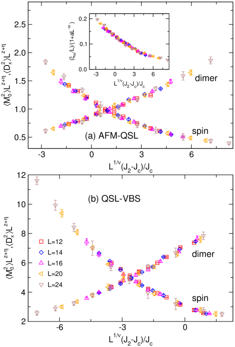
Figure 5: (a) Data collapse of spin and dimer orders for the AFM-QSL transition assuming the critical point located at $J_{c1}=0.45(1)$. (b) Data collapse for the QSL-VBS transition at the critical point $J_{c2}=0.56(1)$. In case (b), dimer order values are magnified by a factor of 20 for a convenient comparison. The inset presents the scaling of the correlation length $\xi_{m}$ at $J_{c1}=0.45$ with $\nu=0.99$, $\omega=2$ and $a=14$.

III Correlation functions in the quantum spin liquid phase

III.1 Spin-spin correlation functions

III.1.1 A detailed comparison between DMRG and PEPS results

To investigate the physical nature of the QSL phase in the maximally frustrated region around $J_{2}\sim 0.5$, we further compute the spin and dimer correlation functions on a strip $L_{y}\times L_{x}$ that is fully open along both $x$ and $y$ directions. We compare the results obtained by DMRG with SU(2) spin rotation symmetry and the finite PEPS ansatz. The correlations are measured along the central line $y=L_{y}/2$ and the distance of the reference site away from the left edge is chosen to be 3 lattice spacings in order to minimize boundary effects.

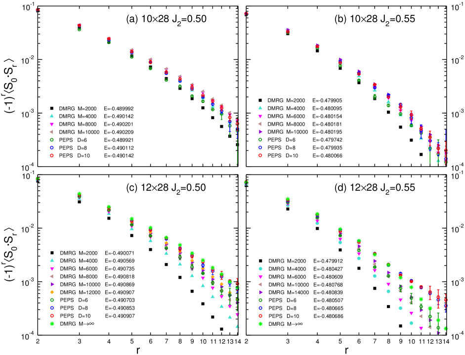
Figure 6: Comparison of spin-spin correlations vs distance obtained in DMRG and PEPS calculations for various bond dimensions $M$ and $D$. $10\times 28$ and $12\times 28$ systems at $J_{2}=0.5$ and $0.55$ are considered in the four panels (a-d). Energies for the different $M$ or $D$ are listed in the corresponding legends for comparison. A log-log plot is used so that the expected power-law behavior in the 2D limit (see text) would show up as a straight line.

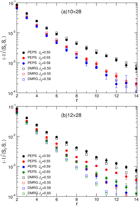
Figure 7: Comparison of the spin correlations vs distance obtained in DMRG and PEPS for different values of $J_{2}$ (semi-log plot). $10\times 28$ (a) and $12\times 28$ (b) strips have been considered. For $10\times 28$, we use $M$=10000. For $12\times 28$, we push $M=14000$ at $J_{2}=0.55$, and $M=12000$ otherwise. PEPS results are obtained with $D=8$.

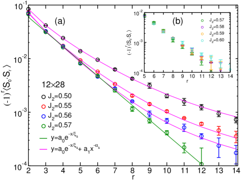
Figure 8: Spin correlation functions on a $12\times 28$ strip computed using a $D=8$ PEPS at different values of $J_{2}$, $J_{2}\leq 0.57$ (a) and $J_{2}\geq 0.57$ (b) (semi-log plots). In (a) different functions are used to fit the spin correlations. The parameters from a two-component fit $y=a_{0}e^{-x/\xi_{s}}+a_{1}x^{-\alpha_{s}}$ used for $J_{2}=0.5$ and 0.55 are listed in Table 2. For $J_{2}=0.57$ the power-law component turns out to have negligible weight and the purely exponential fit $y=a_{0}e^{-x/\xi_{s}}$ gives a correlation length $\xi_{s}=1.59(2)$.

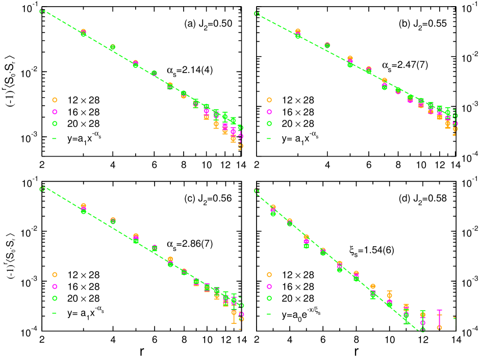
Figure 9: Log-log plot of the spin correlation functions on different system size at (a) $J_{2}=0.5$, (b) $J_{2}=0.55$ and (c) $J_{2}=0.56$, and semi-log plot at (d) $J_{2}=0.58$. Different symbols correspond to different widths $L_{y}$ of the $L_{y}\times 28$ open strip. Black dashed lines denote the fitting curves of $20\times 28$ results with power law fit for (a,b,c) and exponential fit for (d). Corresponding fitting parameters $\alpha_{s}$ or $\xi_{s}$ are given in the figure. The parameters from a two-component fit $y=a_{0}e^{-x/\xi_{s}}+a_{1}x^{-\alpha_{s}}$ (solid lines) used for $J_{2}=0.5$ and $0.55$ (a,b) are listed in Table 2.

Figure 6 depicts the spin correlations versus distance on different systems at two highly frustrated points $J_{2}=0.5$ and $0.55$ on $10\times 28$ and $12\times 28$ systems. DMRG results are obtained with different numbers of SU(2) kept state, as large as $M=14000$ (equivalent to about 56000 U(1) states), and PEPS results are obtained with bond dimension $D$ from 6 to 10. The corresponding ground state energies for different $M$ or $D$ are listed with each legend showing that PEPS and DMRG energies are very close to each other.

For both DMRG and PEPS, by increasing the bond dimensions $M$ or $D$ one improves energies and correlations until convergence. To be more specific, we first focus on PEPS spin correlations. On $10\times 28$ and $12\times 28$ strips, with increasing $D$ from 6 to 10, spin correlations gradually increase but there are few differences between $D=8$ and $D=10$, which indicates $D=8$ already provides converged spin correlations. DMRG correlations also gradually increase with increasing $M$, and it needs larger $M$ to converge the long-distance correlations. Remarkably, as shown in Fig. 6(a) and (b), once convergenced, PEPS and DMRG results on the $L_{y}=10$ strip are in excellent agreement.

However, we find that for $L_{y}$=12, some discrepancies between PEPS and DMRG correlations occur, even when considering the largest bond dimensions $M$ available in DMRG. At $J_{2}=0.5$ there are only small differences for long-distance correlations, but at $J_{2}=0.55$ differences occur already at short-distances while, at long-distance, DMRG correlations are definitely far away from the PEPS results, even when as many as $M=14000$ SU(2) states are kept, as seen in Fig. 6(d). Since the DMRG correlations have not totally converged, we attempt to extrapolate to $M\rightarrow\infty$ with the DMRG correlations at $M=10000$ and $M=14000$ for $J_{2}=0.55$ (or $M=12000$ for $J_{2}=0.5$) through a linear fit in $1/M$, as shown by the green symbols in Fig. 6(c) and (d). For $J_{2}=0.5$ the extrapolated values agree very well with the converged PEPS results. For $J_{2}=0.55$ the extrapolated short-distance correlations also agree well with the PEPS results, while the extrapolated long-distance values are still significantly away, as a result of the inaccuracy of the DMRG extrapolation procedure. Essentially, as a one-dimensional method, DMRG can not capture the correct entanglement structure for large 2D systems, and its accuracy depends strongly on the width $L_{y}$ and the strength of the frustrating $J_{2}$ interaction (here $J_{1}$ is fixed). Increasing $L_{y}$ and $J_{2}$, one needs to keep more states to converge long-distance correlations as well as energies. As the extension of DMRG to higher dimensions, PEPS can capture the correct entanglement structure for 2D systems which satisfies the entanglement entropy’s area law. Therefore, even though PEPS energies are slightly higher, $D=8$ can still produce well-converged correlations at long distance.

To further investigate the influence of $L_{y}$ and $J_{2}$ on the accuracy of DMRG, we compare PEPS spin correlations to DMRG results obtained with the largest available $M$, for different $J_{2}$. On $10\times 28$ we can see PEPS results are in good agreement with DMRG results obtained with $M=10000$ for $J_{2}=0.5$, 0.55 and 0.58, as shown in Fig. 7(a). When increasing $L_{y}$ to 12, as shown in Fig. 7(b), at $J_{2}=0.5$ DMRG and PEPS results correlations still compare well, but for $J_{2}=0.55$, 0.59 and 0.60, discrepancies occur due to lack of convergence of DMRG. In fact, even for the largest available $M$, DMRG tends to underestimate long range spin correlations and, e.g. , gives a clear exponential decay in the suspected critical QSL at $J_{2}=0.55$ where, in contrast, well converged PEPS results are closer to the expected 2D power-law decay (see later for more results). This illustrates the powerful representation ability of PEPS for capturing long-range correlations in large 2D systems. Thus, our results provide the first solid PEPS calculation beyond DMRG.

III.1.2 Power law decay behavior at long distance

From Fig. 6(c) and (d), we note the spin correlations decay much more like in a power law, rather than an exponential form. In order to evidently establish their decay behavior, we plot the spin correlations on the $12\times 28$ open strip from $J_{2}=0.5$ to $0.57$ in Fig. 8(a), and from $J_{2}=0.57$ to $0.60$ in Fig. 8(b). When increasing $J_{2}$ from 0.5 to 0.57, the correlations gradually get smaller. Interestingly, under further increasing $J_{2}$ to 0.60, the correlations seem to get back a little larger. To analyze the correlation behavior in details, we fit the correlations with two different fitting functions, as shown in Fig. 8(a). Comparing the two kinds of fitting functions, we can clearly see that (i) at $J_{2}=0.57$ spin correlations decay exponentially, while (ii) for $J_{2}=0.5$, 0.55 and 0.56 the spin correlations decay with a long tail indicating a power law form.

Table 2: Fitting parameters of the spin-spin correlations on $L_{y}\times 28$ open strips, using the function $y=a_{0}e^{-x/\xi}+a_{1}x^{-\alpha}$.

$J_{2}$	$L_{y}$	$a_{0}$	$a_{1}$	$\xi_{s}$	$\alpha_{s}$
0.50	12	0.095(9)	0.22(2)	1.99(9)	2.16(9)
0.50	16	0.064(13)	0.27(3)	2.07(28)	2.16(13)
0.50	20	0.032(18)	0.31(4)	2.29(98)	2.12(21)
0.55	12	0.107(6)	0.22(1)	1.69(6)	2.50(8)
0.55	16	0.043(29)	0.32(7)	1.74(73)	2.45(35)
0.55	20	0.004(4)	0.39(2)	1.89(87)	2.45(9)

To provide more evidences on the change of behavior of the long distance spin correlations with $J_{2}$, we also consider larger systems up to $20\times 28$. In Fig. 9, we present how the spin correlations vary with increasing system width $L_{y}$. We can see, when increasing $L_{y}$, two different trends of the long-distance spin correlations : at $J_{2}=0.5$, 0.55 and 0.56 the latter increase, while at $J_{2}=0.58$ they decrease. This consolidates our claim of a power law decay behavior for $J_{2}=0.5$, 0.55 and 0.56, and an exponential decay for $J_{2}=0.58$. The power exponents for $J_{2}=0.5$ and 0.55 obtained from the widest $20\times 28$ strip are $\alpha_{s}=2.14(4)$ and $2.47(7)$ respectively, in good agreement with the previous results obtained on the $12\times 28$ strip through a two-component fit. The correlation length at $J_{2}=0.58$ for $20\times 28$ is $\xi_{s}=1.54(6)$, well consistent with the results from $12\times 28$ at $J_{2}=0.57$ . Such results on wide strips confirm and strengthen the previous findings of a gapless QSL and a (gapped) VBS state in the nonmagnetic region, and a phase boundary between the latter at $J_{c2}=0.56$.

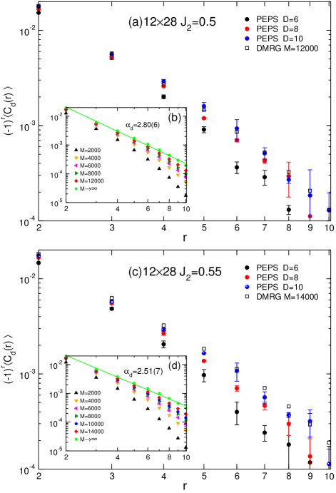
Figure 10: Log-log plot of dimer correlation functions for different system sizes at (a) $J_{2}$=0.5 and (c) $J_{2}$=0.55. The insets (b) and (d) show the DMRG results with different numbers of kept SU(2) states, and the green lines denote the extrapolated DMRG results in the $M\rightarrow\infty$ limit (using a linear fit in $1/M$ and the two largest $M$ values) which are fitted according to a power law in $1/r$. The corresponding exponents $\alpha_{d}$ are indicated in the insets.

III.2 Dimer-dimer correlation functions

To further study the physical properties of the QSL, we also measure the connected dimer-dimer correlations on the central line along the $x$-direction, which is defined as

$$C_{d}(r)=\langle B^{x}_{0}B^{x}_{r}\rangle-\langle B^{x}_{0}\rangle\langle B^{x}_{r}\rangle\,.$$ (7)

The comparison between DMRG and PEPS at $J_{2}=0.5$ and $J_{2}=0.55$ can be found in Fig. 10. We can see that with increasing $D$ or $M$, PEPS and DMRG dimer-dimer correlations will gradually converge, and results of PEPS with $D=10$ are consistent with those of DMRG with the largest available $M$. However, dimer correlations are significantly smaller than spin correlations and are slower to converge in both DMRG and PEPS calculations. In order to estimate the dimer correlations more precisely, we can also extrapolate the dimer correlation values with $M\rightarrow\infty$ from DMRG results, as seen in the insets of Fig. 10 (b) and (d). From the extrapolated DMRG results, we conclude that the dimer-dimer correlations very likely decay as a power law, and exponents $\alpha_{d}=2.80(6)$ and 2.51(7) have been estimated for $J_{2}=0.5$ and 0.55, respectively.

In addition, we also investigate the system size dependence of the local DOP and of its characteristic decay length. The horizontal DOP (hDOP) is defined as the difference $\Delta B$ between nearby strong and weak horizontal bond energies

$$\Delta B(r)=|B^{x}_{r}-B^{x}_{r+e_{x}}|\,.$$ (8)

The hDOP decays exponentially from the left system boundary and the corresponding decay length $\xi_{\rm hDOP}$ can be extracted, as shown in Fig. 11(a). We find that, at $J_{2}=0.5$ and 0.55, the decay length grows linearly with increasing system size, exhibiting the same behavior as that of the RVB state. This is consistent with a power law decay of the dimer-dimer correlation functions in the QSL phase. In contrast, at $J_{2}=0.58$, the growth seems faster, may be superlinear, consistent with the appearance of VBS order in the thermodynamic limit.

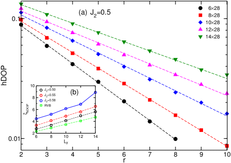
Figure 11: (a) hDOP obtained on different $L_{y}\times 28$ open strips at $J_{2}=0.5$, plotted as a function of the distance from the reference site along the central line $y=L_{y}/2$. The corresponding decay lengths for several width $L_{y}$ are extracted from exponential fits (shown as straight lines). (b) The decay length of the hDOP at $J_{2}=0.5$ and $0.55$ grows linearly with the system width, like for the RVB state. The slopes for RVB, $J_{2}=0.5$ and $0.55$ are 0.301(4), 0.37(1) and 0.39(1), respectively. At $J_{2}=0.58$ a (small) sign of superlinearity is seen.

IV A potential field theory description for the quantum spin liquid phase

To understand the numerical results qualitatively, we start from the well known $CP^{1}$ model description for DQCP between AFM and VBS phases:

$$\mathcal{L}_{\text{DQCP}} = \frac{1}{g}\sum_{a=1}^{2}|(\partial_{\mu}-ia_{\mu})z_{a}|^{2}+m^{2}|z|^{2}+u(|z|^{2})^{2}$$ (9)

$$+ \kappa(\epsilon_{\mu\nu\lambda}\partial_{\nu}a_{\lambda})^{2},$$

where $z_{a}$ is the $CP^{1}$ spinon field and $a_{\mu}$ is the emergent gauge field.

Our numerical results indicate that the QSL state is closely related to the DQCP and it can be regarded as a natural expansion of the DQCP into a stable quantum phase. Then the natural question would be: is there any instability for the usual DQCP scenario such that a stable QSL phase might emerge around it? Here, we conjecture that a topological theta term, or the Hopf term:

$$\mathcal{L}_{\theta}=\frac{\theta}{4\pi^{2}}\epsilon_{\mu\nu\lambda}a_{\mu}\partial_{\nu}a_{\lambda}$$ (10)

with $\theta=\pi$ might do the job. Although in the limit with $J_{2}=0$, it was proven that there is no topological theta term contribution in the usual 2D AFM Heisenberg model Haldane (1988), it is still not clear whether such a term can emerge or not in the presence of bigger $J_{2}$.

According to Polyakov’s early work Polyakov (1988), in the presence of $\mathcal{L}_{\theta}$, the total action $\mathcal{L}_{\text{total}}=\mathcal{L}_{\text{DQCP}}+\mathcal{L}_{\theta}$ is equivalent to four Dirac fermions with short-range interactions. In terms of physical picture, the topological theta term $\mathcal{L}_{\theta}$ leads to the statistical transmutation of spinon excitation in the $CP^{1}$ model. Thus, a power law decay of the spin-spin correlations will be expected at long distance. Due to the square lattice symmetry, the four Dirac spinons will naturally locate at momenta $(\pm\pi/2,\pm\pi/2)$. In Fig.12, we compute the spin structure factor for different $J_{2}$ and we find that subpeaks indeed emerge at momentum point $(0,\pi)$ and $(\pi,0)$ in the QSL regime. We argue that these subpeaks in the spin structure factor might be naturally contributed by those Dirac spinons located at momenta $(\pm\pi/2,\pm\pi/2)$.

On the other hand, since $\mathcal{L}_{\theta}$ will not change the short range physics of the $CP^{1}$ model, the short distance behavior of correlation functions can still be captured by the usual $CP^{1}$ model without $\mathcal{L}_{\theta}$ and that’s why the observed short range spin-spin and dimer-dimer correlations are qualitatively similar to those in the RVB state. (With a two component fitting, we can always find an exponetial decay part for spin-spin correlations for small system size.) In previous works Wang et al. (2013); Qi and Gu (2014); Poilblanc and Mambrini (2017), it has been shown that the RVB state indeed has a very good variational energy around the maximally frustrated region with $J_{2}=0.5$. Thus, we argue that the RVB state can be regarded as a meta-stable state and it naturally serves as the "parent state" for gapless QSL state with power law decay of spin-spin correlation functions.

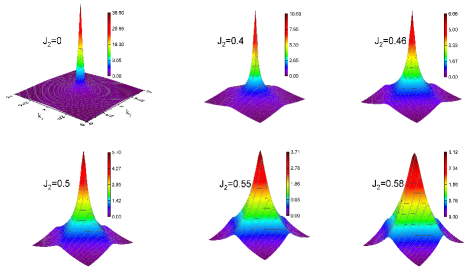
Figure 12: The $\bf k$-space distribution of spin structure factor $S({\bf k})=L^{2}m^{2}_{s}({\bf k})$ at different $J_{2}$ on $L\times L$ systems with $L=20$. Each case shares the same $k_{x}$ and $k_{y}$ axes with the $J_{2}=0$ case, with a peak at ${\bf k}=(\pi,\pi)$.

It is well known that in the DQCP scenario, the bigger anomalous dimension $\eta_{s}$ can be rationalized by the thinking that the Néel order parameter field decays into spinons. Remarkably, we find that $\eta_{s}$ is intrinsically close (comparing systems of similar sizes) to the $J$-$Q$ model value around the AFM-QSL transitions. While for the QSL-VBS transition, $\eta_{d}$ obtained in our numerical calculation also well agrees with the $J$-$Q$ model(again, comparing with similar system size). These two features strongly indicate that the observed QSL might naturally develop from an underlying DQCP. Moreover, we find that $\eta_{s}$ for the QSL-VBS transition is much bigger than the the $J$-$Q$ model and is actually very close to the infinite-$N$ limit of $CP^{N-1}$ model with $\eta_{s}=1$ for QSL-VBS phase transitions. We conjecture that the statistical interaction induced by $\mathcal{L}_{\theta}$ might strongly suppress the quantum fluctuation of $U(1)$ gauge field at QSL-VBS phase transition(confinement transition) and lead to almost "free" fermionic spinon excitations. We will use the large-$N$ expansion to estimate $\eta_{s}$ in the presence of $\mathcal{L}_{\theta}$ term elsewhere. Finally, we stress that the observed correlation exponents $\nu\sim 0.99$ for both AFM-QSL and QSL-VBS transitions might imply the deep relationship between Higgs and confinement transitions of $U(1)$ gauge field. Since $\nu$ is much bigger than those observed in the usual DQCP scenario (comparing systems of similar sizes), e.g., $J$-$Q$ model, we believe that the observed QSL can not be a finite size effect and both transitions must belong to new universality classes which are never observed in other models. Of course, doping the square lattice $J_{1}$-$J_{2}$ model might provide us smoking gun evidence for the emergence of topological theta term and statistic transmutation for spinons, and a d-wave superconductivity could naturally arise. We will also leave this interesting open problem for our future study.

V discussion and conclusion

In summary, applying the state-of-the-art PEPS method to the frustrated $J_{1}$-$J_{2}$ model up to $24\times 24$ open systems, we compute the ground state energies, order parameters and correlation functions with unprecedented precision. Through the analysis of finite-size scaling, our results explicitly show that in the nonmagnetic region $0.45\lesssim J_{2}\leq 0.61$, there exists a gapless QSL phase for $0.45\lesssim J_{2}\lesssim 0.56$ and a weak VBS phase for $0.56\lesssim J_{2}\leq 0.61$. This phase diagram is further supported by the behavior of the spin correlations on wide open strips, which decay as a power law at $J_{2}=0.5$ and 0.55 and exponentially at $J_{2}=0.58$. Besides, the dimer correlations also decay as a power law in the gapless QSL. Furthermore, we also fit the critical exponents at the AFM-QSL and QSL-VBS transitions, which strongly indicates new types of universality class for these two transitions. Finally, we provide a potential quantum field theory framework to understand the physical nature of gapless QSL. We would like to stress that the proposed gapless QSL also gives a concrete example beyond the usual PSG framework.

We stress that our results are among the most reliable on this topic. Besides the excellent accuracy, the very high quanlity of our results is further guaranted by a series of cross checks. These cross checks include: (1) To locate the vanishing point of AFM order, we use the method of finite size scaling analysis of AFM order parameters and the method of the crossing point of a dimensionless quantity $\xi_{m}/L$; (2) To detect the possibility of VBS phase, we use two kinds of VBS order parameters, the one induced by boundaries and the one defined by bond-bond correlations; (3) To locate the VBS-stripe phase transition point, we use stripe order parameter and ground state energy as indepedent approaches. Even for the ground state energy approach, we still use the energy peak position and bulk energy two methods; (4) To determine the decay behaviour of spin-spin correlations, we compute the variation of correlations with system size increasing and we also check how correlations evolve with J2 increasing; (5) To determine the decay behaviour of dimer-dimer correlations, we compute connetced dimer-dimer correlation functions, and we also use the hDOP quantities for further check; (6) We also use different bond dimensions to check the convergence of our results. PEPS and DMRG results, and decay behaviour of correlations and the phase diagrams, respectively, also consist of double check; (7) In the whole process, we also use a well-studied gapless RVB spin liquid state as a reference.

Our high-quality results enable us to put together in a consistent way incomplete and/or seemingly conflicting findings from previous studies. Former vQMC Hu et al. (2013) and recent finite PEPS Liu et al. (2018) studies suggest a gapless QSL but these studies mainly focused on the region $0.4\leq J_{2}\leq 0.55$, and the nature of the ground state in the region $0.55<J_{2}\leq 0.62$ is not carefully studied. An infinite-PEPS (iPEPS) study supports a VBS phase for $0.53\lesssim J_{2}\lesssim 0.61$, but the AFM order vanishes at about $J_{2}=0.53$ Haghshenas and Sheng (2018) which is probably caused by not large enough bond dimension $D$ : iPEPS typically tends to overestimate magnetic correlations and a finite $D$ may induce a spurious finite magnetic order Liao et al. (2017). However, new finite correlation length scaling in iPEPS provides very good results Corboz et al. (2018); Rader and Läuchli (2018), giving a critical value around $J_{c1}\simeq 0.46(1)$ Hasik et al. (2021), in agreement with our findings. It is also very challenging for iPEPS to obtain a gapless QSL Poilblanc and Mambrini (2017), often requiring a very large $D$ to be reached Liao et al. (2017).

In the SU(2)-DMRG study of Ref. Gong et al. (2014), a VBS phase is proposed for $0.5\lesssim J_{2}\lesssim 0.61$, associated with a near critical region $0.44\lesssim J_{2}\lesssim 0.5$. Later, phase diagrams including both spin liquid and VBS phases are suggested in a many-variable vQMC study Morita et al. (2015), which reports a continuous transition between the spin liquid and the VBS at $J_{c2}\simeq 0.5$. Such a phase diagram is also obtained by an indirect approach on the basis of energy level crossing analysis with the most recent DMRG calculations Wang and Sandvik (2018) and another vQMC cacluations Ferrari and Becca (2020), while no clear sign of dimer order is visible in the correlation functions Ferrari and Becca (2020). Our accurate tensor network results up to $24\times 24$ systems evidently establish that both gapless QSL and VBS phase do exist in the nonmagnetic region, supported by the decay behavior of spin-spin and dimer-dimer correlations. Furthermore, we have been able to obtain the critical exponents of the AFM-QSL and QSL-VBS transitions for understanding the nature of the phases.

Very recently, a similar phase diagram was also reached using neural network wave functions Nomura and Imada (2021), i.e., the RBM+PP method, although providing slightly different values of the critical points. In particular, the QSL-VBS transition point is estimated to be $J_{c2}=0.54$ – instead of $J_{c2}=0.56$ here – which seems consistent with another iPEPS result suggesting a very weak VBS (as revealed by a very long dimer correlation length) at $J_{2}=0.55$ Poilblanc et al. (2019). However, without considering a relatively high estimated RBM+PP energy in 2D limit $E_{\rm RBM+PP}\simeq-0.4846$, the RBM+PP energy on large sytems like $16\times 16$ torus $E=-0.4852$ is already higher than our 2D limit energy $E_{\rm PEPS}\simeq-0.4857$, which actually indicates the large size results of RBM+PP are not so accurate as their small size results. Our finite PEPS results, including finite size scaling of order parameters, and the behavior of spin and dimer correlations, all support that the ground state at $J_{2}=0.55$ is critical, consistently with the earlier vQMC results Hu et al. (2013). We note in Ref. Nomura and Imada (2021) the obtained spin and dimer critical exponents $z+\eta_{s1}\approx 1.41$ and $z+\eta_{d1}\approx 1.75$ at the AFM-QSL transition point, and $z+\eta_{s2}\approx 1.60$ and $z+\eta_{d2}\approx 1.44$ at the QSL-VBS transition point, are roughly consistent with our results $z+\eta_{s1}\approx 1.38$ and $z+\eta_{d1}\approx 1.72$ at the AFM-QSL transition point, $z+\eta_{s2}\approx 1.96$ and $z+\eta_{d2}\approx 1.26$ at the QSL-VBS transition point. In Ref. Nomura and Imada (2021), two different correlation length exponents: $\nu=1.21(5)$ at the AFM-QSL and $\nu=0.67(2)$ at the QSL-VBS transition point Nomura and Imada (2021), are obtained by scaling order parameters, but our results find a single correlation length critical exponent $\nu=0.99(6)$ at the two transition points. The disagreement might be caused by the potential accuracy problem on large sizes, as well as the fitting way to extract $\nu$. In Ref. Nomura and Imada (2021), the exponents $z+\eta$ and $\nu$ are fitted by simultaneously adjusting these exponents through scaling the order parameters. In our work, we use the method suggested in Ref. Sandvik (2010b) to extract the exponent $\nu$ first by scaling the correlation length itself, which can avoid simultaneously adjusting other critical exponents. Then a single $\nu=0.99(6)$ is further supported by scaling order parameters. It would be interesting to check the exponent $\nu$ by directly extracting from the correlation length itself in Ref. Nomura and Imada (2021). We would like to point out that from several other frustrated models that also posses AFM-QSL and QSL-VBS transitions, we always observes a single correlation length exponent $\nu\approx 1.0$, which will be published elsewhere Liu et al. (2021b).

Lastly, we note the QSL phase is critical and our computations have been done at a fixed bond dimension $D=8$ and, hence, let us briefly discuss the effect of a finite $D$. Like DMRG, PEPS is belived to work well on the systems whose ground states satisfy the entanglement entropy’s area law by using a (not very large) finite $D$. However, for those systems that do not satisfy the area law including gapless systems, the language of PEPS can also apply well just like what DMRG has ever done. The basic idea is to improve the bond dimension as large as possible and explore reasonable extrapolation techniques. Along this line, the iPEPS method has moved forward a lot by designing efficient algorithms Jiang et al. (2008); Orús and Vidal (2009); Bauer et al. (2011); Xie et al. (2014); Phien et al. (2015); Xie et al. (2017); Fishman et al. (2018); Liao et al. (2019) and developing new theories for extrapolations Corboz et al. (2018); Rader and Läuchli (2018). Besides the popular iPEPS method, the finite PEPS approach here we adopt provides an alternative way. In this context, we aim to accurately simulate the systems as large as possible within the realm of our capability and then use available results for finite size scaling to measure the thermodymic limit properties. Since finite systems would always acquire a gap, we believe there must be a function $D_{\rm min}(L)$ that fixes the minimum $D$ to get D-converged results for a given (linear) system size $L$. We believe $D=8$ here is larger than the necessary bond dimension $D_{\rm min}(L)$ for the largest $L=28$ considered here, so that results are well converged. However, considering larger systems (for even higher accuracy) may require larger $D$ to be converged.

Methodologically, our PEPS calculations provide the first example beyond DMRG of high precision investigation of the $J_{1}$-$J_{2}$ model through one-to-one direct benchmark for small system sizes. Both DMRG and PEPS are theoretically unbiased approaches to deal with finite size frustrated models. However, DMRG is strongly limited to 1D and quasi-1D systems. PEPS is designed for two and higher dimensions, but its power has not been fully demonstrated in numerical simulation until now. The DMRG and PEPS comparisons explicitly show how DMRG gradually fails in 2D, and meanwhile numerically demonstrate the powerful representation ability of PEPS for precisely capturing long-range physics for such highly frustrated 2D systems. It also fills the gap between DMRG and PEPS calculations which always appear separately in previous studies, and thus provides an enlightening approach to understand and check the discrepancies between existing DMRG and 2D tensor network results that are contradictory for other models, which could be crucial to clarify the true nature of a series of controversial quantum many-body problems. The PEPS application here is an excellent prototype on solving long-standing 2D strongly correlated quantum many-body problems by tensor network methods, which we believe will have profound impact on the development of quantum many-body computations and theories. Experimentally, real materials for realizing $J_{1}$-$J_{2}$ model have been explored. A series of compounds with dominant $J_{1}$ and almost negligible $J_{2}$ have been investigated Vaknin et al. (1987); Coldea et al. (2001); Greven et al. (1995); Cuccoli et al. (2003); Tsyrulin et al. (2010); Babkevich et al. (2016); Koga et al. (2016), including the high-Tc superconductivity parent compound $\rm La_{2}CuO_{4}$. The materials with weak $J_{1}$ and strong $J_{2}$ have also been found such as $\rm Sr_{2}CuWO_{6}$, $\rm Li_{2}COMO_{4}$ ($\rm M=Si,Ge$) and $\rm AMoOPO_{4}Cl$ ($\rm A=K,Rb$) in which collinear AFM order is observed Walker et al. (2016); Vasala et al. (2014); Melzi et al. (2001); Rosner et al. (2002, 2003); Ishikawa et al. (2017). But the experimental realization of a $J_{1}$-$J_{2}$ model with the appropriate $J_{2}/J_{1}$ ratio for the highly frustrated region is still very scarce. We hope our theoretical work can attract more attention to further stimulate experimental development on this subject.

VI acknowledgment

We thank helpful discussions with Federico Becca, Ignacio Cirac, Juraj Hasik, Hai-Jun Liao, Yang Qi, Norbert Schuch, Dong-Ning Sheng, Frank Verstraete, Qing-Rui Wang, Xiao-Gang Wen, Fan Yang, and Shuo Yang. We also thank inspiring discussion with Anders Sandvik, and thank Yusuke Normura for helpful discussion and providing raw data. This work is supported by the NSFC/RGC Joint Research Scheme No. N-CUHK427/18, the ANR/RGC Joint Research Scheme No. A-CUHK402/18 from the Hong Kong’s Research Grants Council and the TNSTRONG ANR-16-CE30-0025, TNTOP ANR-18-CE30-0026-01 grants awarded from the French Research Council. Shou-Shu Gong is supported by National Natural Science Foundation of China grants 11874078, 11834014, and the Fundamental Research Funds for the Central Universities. Wei-Qiang Chen is supported by National Key Research and Development Program of China (Grant No. 2016YFA0300300), NSFC (Grants No. 11861161001), the Science, Technology and Innovation Commission of Shenzhen Municipality (No. ZDSYS20190902092905285), and Center for Computational Science and Engineering at Southern University of Science and Technology..

Appendix A Energy convergence

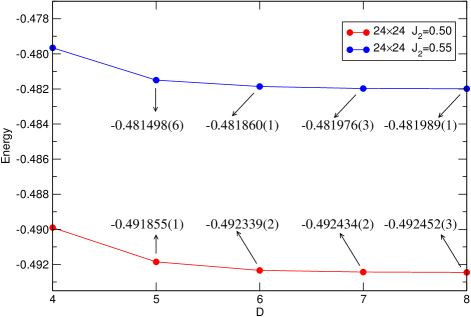
Figure 13: Energy convergence with respect to PEPS bond dimension $D$ on $24\times 24$ at $J_{2}=0.5$ and 0.55. Results using $D=5-8$ are listed.

We show the energy convergence with respect to the bond dimension $D$ on the used largest size $24\times 24$. We choose two typical highly frustrated points $J_{2}=0.5$ and 0.55 as examples, and compare the energies with $D=4-8$. From Fig. 13, we can see when $D$ increases from 4 to 6, the energy decrease is visible. Further increasing $D$ the energy improvement is very small. For example, at $J_{2}=0.55$, the energies with $D=7$ and $D=8$ respectively are $-0.481976(3)$ and $-0.481989(1)$. This indicates $D=8$ can well converge the results.

Appendix B estimated 2D limit energy at $J_{2}=0.5$

We compare the estimated 2D limit energy at $J_{2}=0.5$ from different methods. The 2D limit energy from finite PEPS is $E_{\rm PEPS}=-0.49635(5)$ by finite-size scaling up to $24\times 24$ sites Liu et al. (2021a). From Fig. 14, we can see the energies from cylindrical and periodic boundary conditions are roughly consistent with a $1/L^{3}$ leading scaling. With a linear fit of $1/L^{3}$, the DMRG using $L=8-12$ and vQMC using $L=8-10$ produce almost the same extrapolated energy about $-0.4962$, slightly higher than our finite PEPS 2D limit energy $-0.49635(5)$. The RBM+PP energy on large sizes $L=16$ and $L=18$ are already higher than $E_{\rm PEPS}=-0.49635(5)$, indicating a higher 2D limit energy than $E_{\rm PEPS}$ if the energy increases monotonically with $L$ increasing. Note that $L=16$ energy is slightly higher than that of $L=18$ might be caused by different choices of sublattice structure, the former using $4\times 4$ sublattice and the latter using $6\times 6$ sublattice Nomura and Imada (2021). In anyway, this demonstrates the finite PEPS results indeed have a very good accuracy.

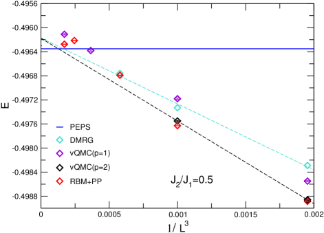
Figure 14: The ground state energy variation with respect to $1/L^{3}$. PEPS 2D limit energy (solid blue line) is shown for comparison. DMRG energies with $L=8-12$ taken from Ref. Gong et al. (2014) use cylindrical boundary condition. vQMC p=1 results with $L=8-18$ and p=2 results with $L=8-10$ taken from Ref. Hu et al. (2013), and RBM+PP results with $L=8-18$ taken from Ref. Nomura and Imada (2021), are based on periodic boundary conditions. Dashed lines denote linear fits versus $1/L^{3}$ for DMRG (cyan) and vQMC p=2 energies (black).

Appendix C collinear AFM phase transition point

Figure 15 depicts the collinear AFM order $M^{2}_{x}=m^{2}_{s}({\pi,0})$ and $M^{2}_{y}=m^{2}_{s}({0,\pi})$ in the region $0.4\leq J_{2}\leq 0.70$. We can see for each size $L\times L$, when $J_{2}$ increases and is larger than some value $J_{c3}(L)$ the system will experience a first-order phase transition and then goes into a collinear AFM phase, characterized by a sudden appearance of the collinear order parameter and explicit symmetry breaking with inequivalent $x$ and $y$ directions. Note that the transition point $J_{c3}(L)$ will get smaller with system size increasing. The transition point $J_{c3}$ in the 2D limit can be evaluated from the transition point $J_{c3}(L)$, which is located at the peak postion of ground state energy function of $L\times L$ sites with respect to $J_{2}$. For example, for $24\times 24$ the phase transition occurs at $J_{c3}$($L$=24) $=0.633$, seen from Fig. 16(a), which shows the $J_{2}$ dependence of energies for each size. A linear fit of $J_{c3}(L)$ versus $1/L$ for $L=10-24$ gives $J_{c3}=0.609(1)$ for $L\rightarrow\infty$, shown in Fig. 16(b). One can also use $L=12-24$ for fitting, giving an extrapolated value $J_{c3}=0.6100(3)$.

Alternatively, the first-order phase transition point $J_{c3}$ in the 2D limit can be estimated only based on the $24\times 24$ open system. As we know, the energy in the 2D limit should be continuous with respect to $J_{2}$ at the phase transition. Generally, given $J_{2}$, the thermodynamic energy $E_{\infty}$ is almost the same as the deep bulk energy $E_{b}$ of an $L\times L$ system, i.e., $E_{\infty}=E_{b}(L)$, if $L$ is large enough, otherwise, finite size effects are still sizable in the bulk and $E_{b}(L)\neq E_{\infty}$. For example, as shown in Fig.16(a), at $J_{2}=0.66$, $E_{\infty}=E_{b}(L)$ is not satisfied for $L=10$ whose first-order transition has not occured, but is true for $L\geq 12$ which has experienced the phase transition. Generally, for $J_{2}\geq J_{c3}(L)$ and $J_{2}\leq J_{c3}$ it has $E_{\infty}=E_{b}(L)$, while for $J_{c3}\leq J_{2}\leq J_{c3}(L)$, $E_{\infty}\neq E_{b}(L)$. Now we use the relation between $E_{\infty}$ and $E_{b}(L)$ to estimate the first-order phase transition point $J_{c3}$ in the 2D limit. We present the total bulk $L\times L$ energy per site and the bulk $(L-8)\times(L-8)$ energy persite $E_{b}(L)$ in Fig. 17. We can see at the transition point $J_{c3}(L$$=$$24)$ $=0.633$, the bulk energy shows a sharp change, which is discontinuous with respect to $J_{2}$, indicating $L=24$ is too small to be used to estimate $E_{\infty}$ for $J_{c3}\leq J_{2}\leq J_{c3}(L$=24). Since $E_{\infty}$ must be continuous w.r.t $J_{2}$, we can obtain the energies $E_{\infty}$ for $J_{c3}\leq J_{2}\leq J_{c3}(L$=24) through the analytic continuation of the energies for $J_{2}>J_{c3}(L$=$24)$. Shown in Fig. 17, the analytic continuation is denoted by a blue dash line, thus the transition point in 2D limit is estimated at $J_{c3}\simeq 0.613$, in good agreement with the above results.

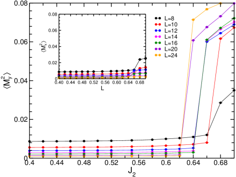
Figure 15: The collinear AFM order parameter $M^{2}_{x}=m^{2}_{s}({\pi,0})$ and $M^{2}_{y}=m^{2}_{s}({0,\pi})$ for different $J_{2}$ on $L\times L$ lattices up to $L=$24 and a PEPS with $D=8$.

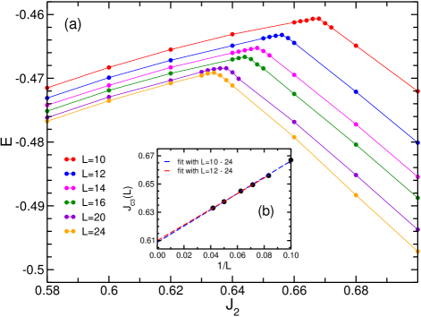
Figure 16: (a) The $J_{2}$ dependence of ground state energies obtained with a $D=8$ PEPS on an $L\times L$ open system, $L=10-24$. For each size, the phase transition point $J_{c2}(L)$ is corresponding to the peak position. (b) The estimation of the transition point in the 2D limit obtained by finite-size scaling of $J_{c3}(L)$ versus $1/L$ through linear fits. The blue line denotes the fit for $L=10-24$ with an extrapolated value 0.609(1), and the red one for $L=12-24$ with an extrapolated value $J_{c3}=0.6100(3)$.

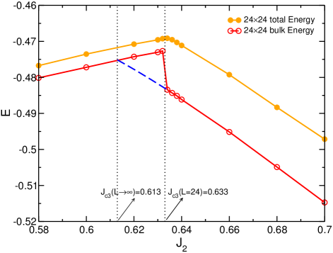
Figure 17: Another approach to estimate the first-order phase transition point $J_{c3}$. The blue dashed line is a third-order polynomial extrapolation from the bulk energies for $J_{2}>0.633$.

Appendix D Comparison of exponents

Using the standard finite-size scaling formula Sandvik (2007); Lou et al. (2009)

$$O(L,J_{2})=L^{-(z+\eta)}F_{O}[L^{1/\nu}(J_{2}-J_{c})/J_{c}]\,,$$ (11)

where $O(L,J_{2})$ is the spin order parameter (squared) $\langle{\bf M}^{2}_{0}\rangle$ or the dimer order parameter (squared) $\langle D^{2}_{x}\rangle$, at the critical point $J_{2}=J_{c}$, one gets $O(L,J_{c})\propto L^{-(1+\eta_{s,d})}$, assuming $z=1$. Therefore, we can compare the critical exponents $\eta_{s,d}$ from the data collapse with the exponents from the scalings $O(L,J_{2})\propto L^{-(1+\eta^{\prime}_{s,d})}$ at different $J_{2}$, to judge the correctness of the critical exponents. It is expected that, when $J_{2}$ gets closer and closer to the critical point $J_{c}$ (within the critical phase), the exponent $\eta^{\prime}_{s,d}$ converges to the critical exponents $\eta_{s,d}$. In Fig. 18, we present the log-log plot of $\langle{\bf M}^{2}_{0}\rangle$ and $\langle D^{2}_{x}\rangle$ versus system size $L$. Exponents at different $J_{2}$ can be easily extracted, and they are listed in Table. 3. It shows that the critical exponents $\eta^{\prime}_{s}$ and $\eta^{\prime}_{d}$ in the critical QSL change continuously between the critical exponents $\eta_{s}$ and $\eta_{d}$, obtained independently for data collapse. Such a consistency demonstrates the reliability of obtaining critical exponents from data collapse.

We can also fit the $\beta$ exponent of the antiferromagnetic order. An easy way to estimate $\beta$ is to use the relation $\beta/\nu=(1+\eta_{s1})/2$, which gives $\beta\approx 0.68$ by using $\eta_{s1}=0.38$ and $\nu=0.99$. We also try to esimate $\beta$ directly from $\langle{\bf M}^{2}_{0}\rangle\sim\Big{(}\frac{J-J_{c1}}{J_{c1}}\Big{)}^{2\beta}$ by using the 2D limit extrapolated magnetic order $\langle{\bf M}^{2}_{0}\rangle$. Shown in Fig. 19, although the 2D $\langle{\bf M}^{2}_{0}\rangle$ values have large error bars, the log-log plot of $\langle{\bf M}^{2}_{0}\rangle$ gives $\beta\approx 0.60$, consistent with the one from the equation $\beta/\nu=(1+\eta_{s1})/2$ .

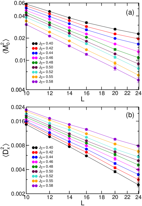
Figure 18: Log-log plot of the AFM order $\langle{\bf M}^{2}_{0}\rangle$ and of the dimer order $\langle D^{2}_{x}\rangle$ versus system size $L$ at different $J_{2}$.

Table 3: Exponents obtained from the scalings $\langle M^{2}_{0}\rangle\propto L^{-(1+\eta^{\prime}_{s})}$ and $\langle D^{2}_{x}\rangle\propto L^{-(1+\eta^{\prime}_{d})}$ at different $J_{2}$ within the critical QSL. The values corresponding to $J_{c1}$ and $J_{c2}$ are the critical exponents $\eta_{s}$ and $\eta_{d}$ obtained from data collapse.

exponent	$J_{c1}$	0.46	0.48	0.50	0.52	0.55	$J_{c2}$
$\eta^{\prime}_{s}$	0.38(3)	0.48(3)	0.61(2)	0.76(1)	0.82(2)	0.91(2)	0.96(4)
$\eta^{\prime}_{d}$	0.72(4)	0.65(1)	0.55(1)	0.49(3)	0.42(2)	0.32(2)	0.26(3)

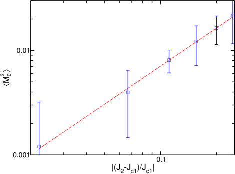
Figure 19: Estimating the $\beta$ exponent from the $L\rightarrow\infty$ extrapolated value of $\langle{\bf M}^{2}_{0}\rangle$ plotted versus the distance from the critical value $J_{c1}=0.45$ in the interval from $J_{2}=0.34$ to $0.44$ (log-log plot).

Appendix E RVB on open boundary finite systems

The resonant valence bond state (RVB) is described by a $D=3$ PEPS with a single tensor and was used to investigate the ground state of the $J_{1}$-$J_{2}$ model at $J_{2}=0.5$. It is a gapless spin liquid state, which has been well studied on cylindrical and periodic systems Wang et al. (2013). On open boundary conditions, we can deal with very large systems with extremely high precision, hence such a state provides an excellent benchmark to study the behavior of spin liquid state on open boundary systems.

First we consider order parameters on $L\times L$ systems up to $40\times 40$ sites. The spin AFM order decreases very rapidly (not shown) consistently with the short-range nature of the spin-spin correlations. Fig. 20(a) shows the finite-size scaling of VBS order patameters, using two definitions, $\langle D^{2}_{\alpha}\rangle$ and $\langle D_{\alpha}\rangle^{2}$. Both of them are zero in the 2D limit. Increasing system size $L$, they decay as $L^{-1.23}$ and $L^{-1.12}$, respectively, as shown in Fig. 20(b). Note that $\langle D^{2}_{\alpha}\rangle$ - based on the bond-bond correlations at all distances and $\langle D_{\alpha}\rangle^{2}$ - induced by the boundaries - are both nonzero (and equal) in VBS states Zhao et al. (2020), but zero in spin liquid states for $L\rightarrow\infty$. Therefore, $\langle D^{2}_{\alpha}\rangle-\langle D_{\alpha}\rangle^{2}$ is always zero in the 2D limit in the VBS and is not a valid VBS order parameter on open boundary systems.

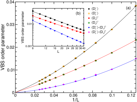
Figure 20: (a) Finite-size scaling of the VBS order parameter of the RVB state on systems with open boundaries with up to $40\times 40$ sites. The extrapolations are performed through a second order polynomial fitting. (b) The log-log plot of order parameters versus system size $L$ .

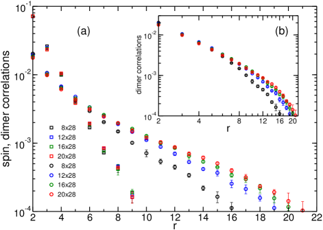
Figure 21: Log-linear plot of spin (square) and dimer correlations (circle) of the RVB state on long strips along the central line $y=L_{y}/2$. The reference site is 3 lattice spacing away from the left edge. The inset shows the dimer correlations on a log-log plot.

As is studied in Ref.Wang et al. (2013) on cylindrical and periodic systems, the spin correlation functions of RVB decay exponentially, and its dimer correlation functions decay as a power law. Now we investigate the spin and dimer correlations on $L_{y}\times L_{x}$ strips to further understand the role of the boundaries, keeping $L_{x}=28$ fixed and varying $L_{y}$. Fig. 21(a) is a log-linear plot of the spin and dimer correlations with respect to the distance $r$. The values of the spin correlations, at all distances, depend barely on the width of the strip, showing a clear exponential decay (with a rather short correlation length). The dimer correlations show a different behavior. Increasing the system width $L_{y}$, we observe that short-distance correlations get smaller and converge but the long-distance ones get larger. So for large systems the dimer correlations will exhibit a long tail, indicating a power law decay. These are special features enabling to distinguish power law from exponential decays. In Fig. 21(b), a log-log plot of the dimer correlations is also shown. It is notable that the long-distance values bend down and show some deviation from a power law, which is just caused by the edge effects from the right open boundary.

Appendix F Extracting decay length of hDOP

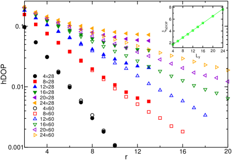
Figure 22: hDOP of the RVB state plotted as a function of the distance from the reference site along the central line $y=L_{y}/2$. Finite size effects on the decay length are controled by comparing results obtained for $L_{x}$ =28 and $60$. The inset shows a linear-linear plot of the hDOP decay length versus system width $L_{y}$.

The horizontal dimer order parameter (hDOP) is defined as the strong and weak energy bond difference (see main text). For long strips with a given system width $L_{y}$, the extracted decay length $\xi_{\rm hDOP}$ of the hDOP may be influenced by the system length $L_{x}$. We first compare the changes of the hDOP of the RVB state for $L_{x}=28$ and $L_{x}=60$, as shown in Fig. 22. We can see that, for $L_{y}\geq 16$, one needs a relative large value of $L_{x}$ such as $L_{x}=60$ to minimize finite-size effects on $\xi_{\rm hDOP}$, while, for the other cases, $L_{x}=28$ is long enough to obtain the correct decay length. For the $J_{1}$-$J_{2}$ model, we compare the hDOP on $L_{x}=28$ and $L_{x}=2L_{y}$, as shown in Fig. 23. It can be seen that $L_{x}=28$ is long enough to extract $\xi_{\rm hDOP}$ by using the hDOP values from $r\leq 7$, for all cases.

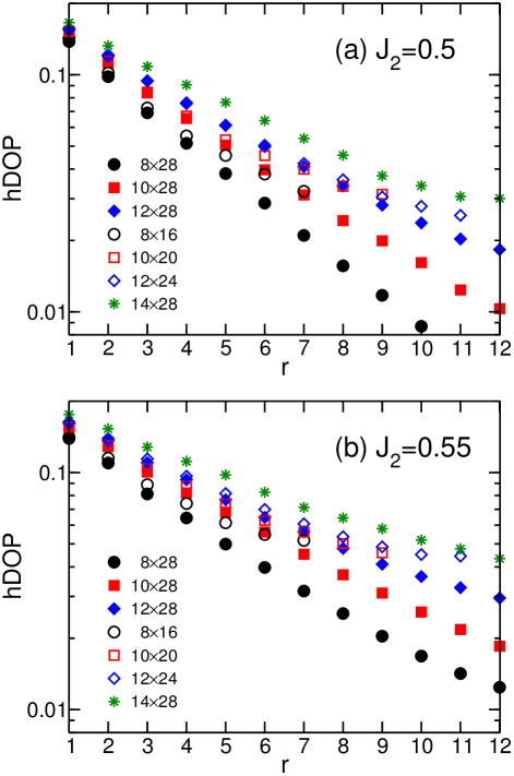
Figure 23: hDOP plotted as a function of the distance from the reference site along the central line $y=L_{y}/2$, for the $J_{1}$-$J_{2}$ model at $J_{2}=0.5$ (a) and $0.55$ (b), computed with a $D=8$ PEPS. Lengths $L_{x}=2L_{y}$ and $L_{x}=28$ are considered, to control the effect of a finite $L_{x}$.

Appendix G Spin correlations at different $J_{2}$

Here we study the finite-size effects on the spin correlations in the QSL and the VBS phases. Spin correlations obtained on long $L_{y}\times 28$ open strips, for different $J_{2}$ values, are shown in Fig. 24. In the narrowest strip, $L_{y}=4$, the correlations vary only slightly in the range $J_{2}=0.5-0.6$. Increasing the width to $L_{y}=8$, the correlations at $J_{2}=0.5$ start to deviate from the other ones in the range $J_{2}=0.55-0.6$. Further increasing $L_{y}$ to 12, 16 and 20, we can see that the behaviors at $J_{2}=0.5$ and $0.55$, on one hand, and at $J_{2}=0.57-0.60$, on the other hand, deviates qualitatively, showing different decay behavior. Also data obtained for $L_{y}=12$, $16$ and $20$ are quantitatively quite close, indicating small remaining finite-size effects in contrast to $L_{y}=4$ and $8$. In addition, note that, the spin correlations show very fast decay within the interval from $J_{2}=J_{c2}$ to 0.6, possibly fastest around $J_{2}=0.58$. indicating a minimum of the correlation length (or equivalently a maximum of the triplet gap) in the VBS phase.

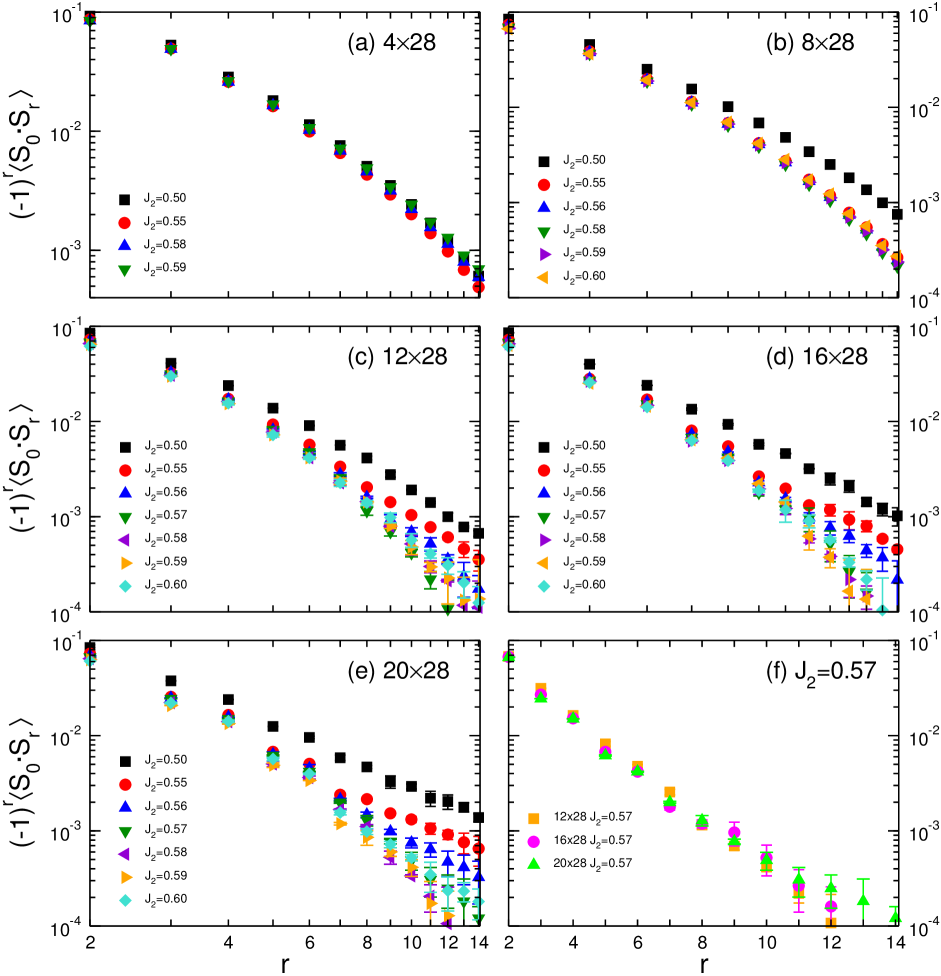
Figure 24: Log-log plot of spin-spin correlation functions at different $J_{2}$ ranging from 0.5 to 0.6 for $L_{y}\times L_{x}$ systems with $L_{y}=4$ (a), $L_{y}=8$ (b), $L_{y}=12$ (c), $L_{y}=16$ (d) and $L_{y}=20$ (e). As a comparison, we also use the semi-log plot for the spin-spin correlation functions at $J_{2}=0.57$ with different values of $L_{y}$ (f). We (very crudely) estimate the spin correlation length is $\xi\sim 2.2(3)$ for $L_{y}=20$. (a,b) have been obtained using SU(2)-DMRG and (c,d,e,f) using a $D=8$ PEPS.

References

- Anderson (1987) P. W. Anderson, “The resonating valence bond state in and superconductivity,” Science 235, 1196–1198 (1987).
- Wen et al. (1989) X. G. Wen, Frank Wilczek, and A. Zee, “Chiral spin states and superconductivity,” Phys. Rev. B 39, 11413–11423 (1989).
- Read and Sachdev (1991) N. Read and Subir Sachdev, “Large-N expansion for frustrated quantum antiferromagnets,” Phys. Rev. Lett. 66, 1773–1776 (1991).
- Lee et al. (2006) Patrick A. Lee, Naoto Nagaosa, and Xiao-Gang Wen, “Doping a mott insulator: Physics of high-temperature superconductivity,” Rev. Mod. Phys. 78, 17–85 (2006).
- Poilblanc et al. (2014) Didier Poilblanc, Philippe Corboz, Norbert Schuch, and J. Ignacio Cirac, “Resonating-valence-bond superconductors with fermionic projected entangled pair states,” Phys. Rev. B 89, 241106 (2014).
- Chandra and Doucot (1988) P. Chandra and B. Doucot, “Possible spin-liquid state at large for the frustrated square Heisenberg lattice,” Phys. Rev. B 38, 9335–9338 (1988).
- Dagotto and Moreo (1989) Elbio Dagotto and Adriana Moreo, “Phase diagram of the frustrated spin-1/2 Heisenberg antiferromagnet in 2 dimensions,” Phys. Rev. Lett. 63, 2148–2151 (1989).
- Figueirido et al. (1990) F. Figueirido, A. Karlhede, S. Kivelson, S. Sondhi, M. Rocek, and D. S. Rokhsar, “Exact diagonalization of finite frustrated spin-1/2 Heisenberg models,” Phys. Rev. B 41, 4619–4632 (1990).
- Sachdev and Bhatt (1990) Subir Sachdev and R. N. Bhatt, “Bond-operator representation of quantum spins: Mean-field theory of frustrated quantum Heisenberg antiferromagnets,” Phys. Rev. B 41, 9323–9329 (1990).
- Poilblanc et al. (1991) Didier Poilblanc, Eduardo Gagliano, Silvia Bacci, and Elbio Dagotto, “Static and dynamical correlations in a spin-1/2 frustrated antiferromagnet,” Phys. Rev. B 43, 10970–10983 (1991).
- Chubukov and Jolicoeur (1991) Andrey V. Chubukov and Th. Jolicoeur, “Dimer stability region in a frustrated quantum Heisenberg antiferromagnet,” Phys. Rev. B 44, 12050–12053 (1991).
- Schulz and Ziman (1992) H. J Schulz and T. A. L Ziman, “Finite-size scaling for the two-dimensional frustrated quantum Heisenberg antiferromagnet,” Europhysics Letters 18, 355–360 (1992).
- Ivanov and Ivanov (1992) N. B. Ivanov and P. Ch. Ivanov, “Frustrated two-dimensional quantum Heisenberg antiferromagnet at low temperatures,” Phys. Rev. B 46, 8206–8213 (1992).
- Einarsson and Schulz (1995) T. Einarsson and H. J. Schulz, “Direct calculation of the spin stiffness in the Heisenberg antiferromagnet,” Phys. Rev. B 51, 6151–6154 (1995).
- H. J. Schulz and Poilblanc (1996) T. A. L. Ziman H. J. Schulz and D. Poilblanc, “Magnetic order and disorder in the frustrated quantum Heisenberg antiferromagnet in two dimensions,” J. Phys. I 6, 675–703 (1996).
- Zhitomirsky and Ueda (1996) M. E. Zhitomirsky and Kazuo Ueda, “Valence-bond crystal phase of a frustrated spin-1/2 square-lattice antiferromagnet,” Phys. Rev. B 54, 9007–9010 (1996).
- Singh et al. (1999) Rajiv R. P. Singh, Zheng Weihong, C. J. Hamer, and J. Oitmaa, “Dimer order with striped correlations in the - Heisenberg model,” Phys. Rev. B 60, 7278–7283 (1999).
- Capriotti and Sorella (2000) Luca Capriotti and Sandro Sorella, “Spontaneous plaquette dimerization in the - Heisenberg model,” Phys. Rev. Lett. 84, 3173–3176 (2000).
- Capriotti et al. (2001) Luca Capriotti, Federico Becca, Alberto Parola, and Sandro Sorella, “Resonating valence bond wave functions for strongly frustrated spin systems,” Phys. Rev. Lett. 87, 097201 (2001).
- Zhang et al. (2003) Guang-Ming Zhang, Hui Hu, and Lu Yu, “Valence-bond spin-liquid state in two-dimensional frustrated spin- Heisenberg antiferromagnets,” Phys. Rev. Lett. 91, 067201 (2003).
- Takano et al. (2003) Ken’ichi Takano, Yoshiya Kito, Yoshiaki Ōno, and Kazuhiro Sano, “Nonlinear model method for the - Heisenberg model: Disordered ground state with plaquette symmetry,” Phys. Rev. Lett. 91, 197202 (2003).
- Sirker et al. (2006) J. Sirker, Zheng Weihong, O. P. Sushkov, and J. Oitmaa, “ model: First-order phase transition versus deconfinement of spinons,” Phys. Rev. B 73, 184420 (2006).
- Schmalfuß et al. (2006) D. Schmalfuß, R. Darradi, J. Richter, J. Schulenburg, and D. Ihle, “Quantum - antiferromagnet on a stacked square lattice: Influence of the interlayer coupling on the ground-state magnetic ordering,” Phys. Rev. Lett. 97, 157201 (2006).
- Mambrini et al. (2006) Matthieu Mambrini, Andreas Läuchli, Didier Poilblanc, and Frédéric Mila, “Plaquette valence-bond crystal in the frustrated Heisenberg quantum antiferromagnet on the square lattice,” Phys. Rev. B 74, 144422 (2006).
- Darradi et al. (2008) R. Darradi, O. Derzhko, R. Zinke, J. Schulenburg, S. E. Krüger, and J. Richter, “Ground state phases of the spin-1/2 - Heisenberg antiferromagnet on the square lattice: A high-order coupled cluster treatment,” Phys. Rev. B 78, 214415 (2008).
- Arlego and Brenig (2008) Marcelo Arlego and Wolfram Brenig, “Plaquette order in the -- model: Series expansion analysis,” Phys. Rev. B 78, 224415 (2008).
- Isaev et al. (2009) L. Isaev, G. Ortiz, and J. Dukelsky, “Hierarchical mean-field approach to the - Heisenberg model on a square lattice,” Phys. Rev. B 79, 024409 (2009).
- Murg et al. (2009) V. Murg, F. Verstraete, and J. I. Cirac, “Exploring frustrated spin systems using projected entangled pair states,” Phys. Rev. B 79, 195119 (2009).
- Beach (2009) K. S. D. Beach, “Master equation approach to computing rvb bond amplitudes,” Phys. Rev. B 79, 224431 (2009).
- Richter and Schulenburg (2010) J. Richter and J. Schulenburg, “The spin-1/2 Heisenberg antiferromagnet on the square lattice: Exact diagonalization for spins,” The European Physical Journal B 73, 117 (2010).
- Yu and Kao (2012) Ji-Feng Yu and Ying-Jer Kao, “Spin- - Heisenberg antiferromagnet on a square lattice: A plaquette renormalized tensor network study,” Phys. Rev. B 85, 094407 (2012).
- Jiang et al. (2012) Hong-Chen Jiang, Hong Yao, and Leon Balents, “Spin liquid ground state of the spin- square - Heisenberg model,” Phys. Rev. B 86, 024424 (2012).
- Mezzacapo (2012) Fabio Mezzacapo, “Ground-state phase diagram of the quantum - model on the square lattice,” Phys. Rev. B 86, 045115 (2012).
- Wang et al. (2013) Ling Wang, Didier Poilblanc, Zheng-Cheng Gu, Xiao-Gang Wen, and Frank Verstraete, “Constructing a gapless spin-liquid state for the spin- - Heisenberg model on a square lattice,” Phys. Rev. Lett. 111, 037202 (2013).
- Hu et al. (2013) Wen-Jun Hu, Federico Becca, Alberto Parola, and Sandro Sorella, “Direct evidence for a gapless spin liquid by frustrating néel antiferromagnetism,” Phys. Rev. B 88, 060402 (2013).
- Doretto (2014) R. L. Doretto, “Plaquette valence-bond solid in the square-lattice - antiferromagnet Heisenberg model: A bond operator approach,” Phys. Rev. B 89, 104415 (2014).
- Qi and Gu (2014) Yang Qi and Zheng-Cheng Gu, “Continuous phase transition from néel state to spin-liquid state on a square lattice,” Phys. Rev. B 89, 235122 (2014).
- Gong et al. (2014) Shou-Shu Gong, Wei Zhu, D. N. Sheng, Olexei I. Motrunich, and Matthew P. A. Fisher, “Plaquette ordered phase and quantum phase diagram in the spin- - square Heisenberg model,” Phys. Rev. Lett. 113, 027201 (2014).
- Chou and Chen (2014) Chung-Pin Chou and Hong-Yi Chen, “Simulating a two-dimensional frustrated spin system with fermionic resonating-valence-bond states,” Phys. Rev. B 90, 041106 (2014).
- Morita et al. (2015) Satoshi Morita, Ryui Kaneko, and Masatoshi Imada, “Quantum spin liquid in spin 1/2 - Heisenberg model on square lattice: Many-variable variational monte carlo study combined with quantum-number projections,” Journal of the Physical Society of Japan 84, 024720 (2015).
- Richter et al. (2015) Johannes Richter, Ronald Zinke, and Damian J. J. Farnell, “The spin-1/2 square-lattice - model: the spin-gap issue,” The European Physical Journal B 88, 2 (2015).
- Wang et al. (2016) Ling Wang, Zheng-Cheng Gu, Frank Verstraete, and Xiao-Gang Wen, “Tensor-product state approach to spin- square - antiferromagnetic Heisenberg model: Evidence for deconfined quantum criticality,” Phys. Rev. B 94, 075143 (2016).
- Poilblanc and Mambrini (2017) Didier Poilblanc and Matthieu Mambrini, “Quantum critical phase with infinite projected entangled paired states,” Phys. Rev. B 96, 014414 (2017).
- Wang and Sandvik (2018) Ling Wang and Anders W. Sandvik, “Critical level crossings and gapless spin liquid in the square-lattice spin- - Heisenberg antiferromagnet,” Phys. Rev. Lett. 121, 107202 (2018).
- Haghshenas and Sheng (2018) R. Haghshenas and D. N. Sheng, “-symmetric infinite projected entangled-pair states study of the spin-1/2 square - Heisenberg model,” Phys. Rev. B 97, 174408 (2018).
- Liu et al. (2018) Wen-Yuan Liu, Shaojun Dong, Chao Wang, Yongjian Han, Hong An, Guang-Can Guo, and Lixin He, “Gapless spin liquid ground state of the spin- - Heisenberg model on square lattices,” Phys. Rev. B 98, 241109 (2018).
- Poilblanc et al. (2019) Didier Poilblanc, Matthieu Mambrini, and Sylvain Capponi, “Critical colored-RVB states in the frustrated quantum Heisenberg model on the square lattice,” SciPost Phys. 7, 41 (2019).
- Ferrari and Becca (2020) Francesco Ferrari and Federico Becca, “Gapless spin liquid and valence-bond solid in the - heisenberg model on the square lattice: Insights from singlet and triplet excitations,” Phys. Rev. B 102, 014417 (2020).
- Nomura and Imada (2021) Yusuke Nomura and Masatoshi Imada, “Dirac-type nodal spin liquid revealed by refined quantum many-body solver using neural-network wave function, correlation ratio, and level spectroscopy,” Phys. Rev. X 11, 031034 (2021).
- Wen (1991) X. G. Wen, “Mean-field theory of spin-liquid states with finite energy gap and topological orders,” Phys. Rev. B 44, 2664–2672 (1991).
- Barkeshli et al. (2019) Maissam Barkeshli, Parsa Bonderson, Meng Cheng, and Zhenghan Wang, “Symmetry fractionalization, defects, and gauging of topological phases,” Phys. Rev. B 100, 115147 (2019).
- Senthil et al. (2004a) T. Senthil, Ashvin Vishwanath, Leon Balents, Subir Sachdev, and Matthew P. A. Fisher, “Deconfined quantum critical points,” Science 303, 1490–1494 (2004a).
- Senthil et al. (2004b) T. Senthil, Leon Balents, Subir Sachdev, Ashvin Vishwanath, and Matthew P. A. Fisher, “Quantum criticality beyond the landau-ginzburg-wilson paradigm,” Phys. Rev. B 70, 144407 (2004b).
- Sandvik (2007) Anders W. Sandvik, “Evidence for deconfined quantum criticality in a two-dimensional Heisenberg model with four-spin interactions,” Phys. Rev. Lett. 98, 227202 (2007).
- Sandvik (2010a) Anders W. Sandvik, “Continuous quantum phase transition between an antiferromagnet and a valence-bond solid in two dimensions: Evidence for logarithmic corrections to scaling,” Phys. Rev. Lett. 104, 177201 (2010a).
- Nahum et al. (2015) Adam Nahum, J. T. Chalker, P. Serna, M. Ortuño, and A. M. Somoza, “Deconfined quantum criticality, scaling violations, and classical loop models,” Phys. Rev. X 5, 041048 (2015).
- Shao et al. (2016) Hui Shao, Wenan Guo, and Anders W. Sandvik, “Quantum criticality with two length scales,” Science 352, 213–216 (2016).
- Lou et al. (2009) Jie Lou, Anders W. Sandvik, and Naoki Kawashima, “Antiferromagnetic to valence-bond-solid transitions in two-dimensional Heisenberg models with multispin interactions,” Phys. Rev. B 80, 180414 (2009).
- Sandvik and Zhao (2020) Anders W. Sandvik and Bowen Zhao, “Consistent scaling exponents at the deconfined quantum-critical point,” Chinese Physics Letters 37, 057502 (2020).
- Verstraete and Cirac (2004) F. Verstraete and J. I. Cirac, “Renormalization algorithms for quantum-many body systems in two and higher dimensions,” (2004), arXiv:cond-mat/0407066 [cond-mat.str-el] .
- Verstraete et al. (2006) F. Verstraete, M. M. Wolf, D. Perez-Garcia, and J. I. Cirac, “Criticality, the area law, and the computational power of projected entangled pair states,” Phys. Rev. Lett. 96, 220601 (2006).
- Verstraete et al. (2008) F. Verstraete, V. Murg, and J.I. Cirac, “Matrix product states, projected entangled pair states, and variational renormalization group methods for quantum spin systems,” Advances in Physics 57, 143–224 (2008).
- Sandvik and Vidal (2007) A. W. Sandvik and G. Vidal, “Variational quantum monte carlo simulations with tensor-network states,” Phys. Rev. Lett. 99, 220602 (2007).
- Schuch et al. (2008) Norbert Schuch, Michael M. Wolf, Frank Verstraete, and J. Ignacio Cirac, “Simulation of quantum many-body systems with strings of operators and monte carlo tensor contractions,” Phys. Rev. Lett. 100, 040501 (2008).
- Sandvik (2008) Anders W. Sandvik, “Scale-renormalized matrix-product states for correlated quantum systems,” Phys. Rev. Lett. 101, 140603 (2008).
- Wang et al. (2011) Ling Wang, Iztok Pižorn, and Frank Verstraete, “Monte carlo simulation with tensor network states,” Phys. Rev. B 83, 134421 (2011).
- Liu et al. (2017) Wen-Yuan Liu, Shao-Jun Dong, Yong-Jian Han, Guang-Can Guo, and Lixin He, “Gradient optimization of finite projected entangled pair states,” Phys. Rev. B 95, 195154 (2017).
- Liu et al. (2021a) Wen-Yuan Liu, Yi-Zhen Huang, Shou-Shu Gong, and Zheng-Cheng Gu, “Accurate simulation for finite projected entangled pair states in two dimensions,” Phys. Rev. B 103, 235155 (2021a).
- Stoudenmire and White (2012) E.M. Stoudenmire and Steven R. White, “Studying two-dimensional systems with the density matrix renormalization group,” Annual Review of Condensed Matter Physics 3, 111–128 (2012).
- Sandvik (2010b) Anders W. Sandvik, “Computational studies of quantum spin systems,” AIP Conference Proceedings 1297, 135–338 (2010b).
- Zhao et al. (2020) Bowen Zhao, Jun Takahashi, and Anders W. Sandvik, “Comment on “gapless spin liquid ground state of the spin- - Heisenberg model on square lattices”,” Phys. Rev. B 101, 157101 (2020).
- Kaul (2015) Ribhu K. Kaul, “Spin nematics, valence-bond solids, and spin liquids in quantum spin models on the triangular lattice,” Phys. Rev. Lett. 115, 157202 (2015).
- Note (1) The estimation of at is subject to finite- effects and that the thermodynamic value of is expected to be significantly larger than the value extracted from Fig. 8(a) for , as is seen from Fig. 24(f).
- Haldane (1988) F. D. M. Haldane, “O(3) nonlinear model and the topological distinction between integer- and half-integer-spin antiferromagnets in two dimensions,” Phys. Rev. Lett. 61, 1029–1032 (1988).
- Polyakov (1988) A. M. Polyakov, “Fermi-bose transmutation induced by gauge field,” Mordern Physics Letters A 3, 325–328 (1988).
- Liao et al. (2017) H. J. Liao, Z. Y. Xie, J. Chen, Z. Y. Liu, H. D. Xie, R. Z. Huang, B. Normand, and T. Xiang, “Gapless spin-liquid ground state in the kagome antiferromagnet,” Phys. Rev. Lett. 118, 137202 (2017).
- Corboz et al. (2018) Philippe Corboz, Piotr Czarnik, Geert Kapteijns, and Luca Tagliacozzo, “Finite correlation length scaling with infinite projected entangled-pair states,” Phys. Rev. X 8, 031031 (2018).
- Rader and Läuchli (2018) Michael Rader and Andreas M. Läuchli, “Finite correlation length scaling in lorentz-invariant gapless iPEPS wave functions,” Phys. Rev. X 8, 031030 (2018).
- Hasik et al. (2021) Juraj Hasik, Didier Poilblanc, and Federico Becca, “Investigation of the Néel phase of the frustrated Heisenberg antiferromagnet by differentiable symmetric tensor networks,” SciPost Phys. 10, 12 (2021).
- Liu et al. (2021b) Wen-Yuan Liu, Juraj Hasik, Shou-Shu Gong, Didier Poilblanc, Wei-Qiang Chen, and Zheng-Cheng Gu, “The emergence of gapless quantum spin liquid from deconfined quantum critical point,” (2021b), arXiv:2110.11138 [cond-mat.str-el] .
- Jiang et al. (2008) H. C. Jiang, Z. Y. Weng, and T. Xiang, “Accurate determination of tensor network state of quantum lattice models in two dimensions,” Phys. Rev. Lett. 101, 090603 (2008).
- Orús and Vidal (2009) Román Orús and Guifré Vidal, “Simulation of two-dimensional quantum systems on an infinite lattice revisited: Corner transfer matrix for tensor contraction,” Phys. Rev. B 80, 094403 (2009).
- Bauer et al. (2011) B. Bauer, P. Corboz, R. Orús, and M. Troyer, “Implementing global abelian symmetries in projected entangled-pair state algorithms,” Phys. Rev. B 83, 125106 (2011).
- Xie et al. (2014) Z. Y. Xie, J. Chen, J. F. Yu, X. Kong, B. Normand, and T. Xiang, “Tensor renormalization of quantum many-body systems using projected entangled simplex states,” Phys. Rev. X 4, 011025 (2014).
- Phien et al. (2015) Ho N. Phien, Johann A. Bengua, Hoang D. Tuan, Philippe Corboz, and Román Orús, “Infinite projected entangled pair states algorithm improved: Fast full update and gauge fixing,” Phy. Rev. B 92, 035142 (2015).
- Xie et al. (2017) Z. Y. Xie, H. J. Liao, R. Z. Huang, H. D. Xie, J. Chen, Z. Y. Liu, and T. Xiang, “Optimized contraction scheme for tensor-network states,” Phy. Rev. B 96, 045128 (2017).
- Fishman et al. (2018) M. T. Fishman, L. Vanderstraeten, V. Zauner-Stauber, J. Haegeman, and F. Verstraete, “Faster methods for contracting infinite two-dimensional tensor networks,” Phys. Rev. B 98, 235148 (2018).
- Liao et al. (2019) Hai-Jun Liao, Jin-Guo Liu, Lei Wang, and Tao Xiang, “Differentiable programming tensor networks,” Physical Review X 9 (2019), 10.1103/physrevx.9.031041.
- Vaknin et al. (1987) D. Vaknin, S. K. Sinha, D. E. Moncton, D. C. Johnston, J. M. Newsam, C. R. Safinya, and H. E. King, “Antiferromagnetism in ,” Phys. Rev. Lett. 58, 2802–2805 (1987).
- Coldea et al. (2001) R. Coldea, S. M. Hayden, G. Aeppli, T. G. Perring, C. D. Frost, T. E. Mason, S.-W. Cheong, and Z. Fisk, “Spin waves and electronic interactions in ,” Phys. Rev. Lett. 86, 5377–5380 (2001).
- Greven et al. (1995) M. Greven, R.J. Birgeneau, Y. Endoh, M. A. Kastner, M. Matsuda, and G. Shirane, “Neutron scattering study of the two-dimensional spins=1/2 square-lattice Heisenberg antiferromagnet ,” Z. Physik B - Condensed Matter 96, 465–477 (1995).
- Cuccoli et al. (2003) Alessandro Cuccoli, Tommaso Roscilde, Ruggero Vaia, and Paola Verrucchi, “Detection of XY behavior in weakly anisotropic quantum antiferromagnets on the square lattice,” Phys. Rev. Lett. 90, 167205 (2003).
- Tsyrulin et al. (2010) N. Tsyrulin, F. Xiao, A. Schneidewind, P. Link, H. M. Rønnow, J. Gavilano, C. P. Landee, M. M. Turnbull, and M. Kenzelmann, “Two-dimensional square-lattice antiferromagnet ,” Phys. Rev. B 81, 134409 (2010).
- Babkevich et al. (2016) P. Babkevich, Vamshi M. Katukuri, B. Fåk, S. Rols, T. Fennell, D. Pajić, H. Tanaka, T. Pardini, R. R. P. Singh, A. Mitrushchenkov, O. V. Yazyev, and H. M. Rønnow, “Magnetic excitations and electronic interactions in : A spin- square lattice Heisenberg antiferromagnet,” Phys. Rev. Lett. 117, 237203 (2016).
- Koga et al. (2016) Tomoyuki Koga, Nobuyuki Kurita, Maxim Avdeev, Sergey Danilkin, Taku J. Sato, and Hidekazu Tanaka, “Magnetic structure of the quasi-two-dimensional square-lattice Heisenberg antiferromagnet ,” Phys. Rev. B 93, 054426 (2016).
- Walker et al. (2016) H. C. Walker, O. Mustonen, S. Vasala, D. J. Voneshen, M. D. Le, D. T. Adroja, and M. Karppinen, “Spin wave excitations in the tetragonal double perovskite ,” Phys. Rev. B 94, 064411 (2016).
- Vasala et al. (2014) S Vasala, M Avdeev, S Danilkin, O Chmaissem, and M Karppinen, “Magnetic structure of ,” Journal of Physics: Condensed Matter 26, 496001 (2014).
- Melzi et al. (2001) R. Melzi, S. Aldrovandi, F. Tedoldi, P. Carretta, P. Millet, and F. Mila, “Magnetic and thermodynamic properties of : A two-dimensional frustrated antiferromagnet on a square lattice,” Phys. Rev. B 64, 024409 (2001).
- Rosner et al. (2002) H. Rosner, R. R. P. Singh, W. H. Zheng, J. Oitmaa, S.-L. Drechsler, and W. E. Pickett, “Realization of a large quasi-2d spin-half Heisenberg system: ,” Phys. Rev. Lett. 88, 186405 (2002).
- Rosner et al. (2003) H. Rosner, R. R. P. Singh, W. H. Zheng, J. Oitmaa, and W. E. Pickett, “High-temperature expansions for the - Heisenberg models: Applications to ab initio calculated models for and ,” Phys. Rev. B 67, 014416 (2003).
- Ishikawa et al. (2017) Hajime Ishikawa, Nanako Nakamura, Makoto Yoshida, Masashi Takigawa, Peter Babkevich, Navid Qureshi, Henrik M. Rønnow, Takeshi Yajima, and Zenji Hiroi, “- square-lattice Heisenberg antiferromagnets with spins: ,” Phys. Rev. B 95, 064408 (2017).