CNN-Based Ultrasound Image Reconstruction for Ultrafast Displacement Tracking

Abstract

Thanks to its capability of acquiring full-view frames at multiple kilohertz, ultrafast us imaging unlocked the analysis of rapidly changing physical phenomena in the human body, with pioneering applications such as ultrasensitive flow imaging in the cardiovascular system or shear-wave elastography. The accuracy achievable with these motion estimation techniques is strongly contingent upon two contradictory requirements: a high quality of consecutive frames and a high frame rate. Indeed, the image quality can usually be improved by increasing the number of steered ultrafast acquisitions, but at the expense of a reduced frame rate and possible motion artifacts. To achieve accurate motion estimation at uncompromised frame rates and immune to motion artifacts, the proposed approach relies on single ultrafast acquisitions to reconstruct high-quality frames and on only two consecutive frames to obtain 2-D displacement estimates. To this end, we deployed a cnn-based image reconstruction method combined with a speckle tracking algorithm based on cross-correlation. Numerical and in vivo experiments, conducted in the context of plane-wave imaging, demonstrate that the proposed approach is capable of estimating displacements in regions where the presence of sl and gl artifacts prevents any displacement estimation with a state-of-the-art technique that relies on conventional das beamforming. The proposed approach may therefore unlock the full potential of ultrafast ultrasound, in applications such as ultrasensitive cardiovascular motion and flow analysis or shear-wave elastography.

Biomedical imaging, deep learning, diffraction artifacts, displacement estimation, image reconstruction, speckle tracking, ultrafast ultrasound imaging.

1 Introduction

Ultrafast ultrasound (US) imaging enables reconstructing full-view images from single acquisitions by insonifying the entire field of view at once, using unfocused transmit wavefronts such as plane waves (PWs) or diverging waves (DWs) [1]. us images are then reconstructed from the received echo signals using the well-known delay-and-sum (DAS) algorithm. Ultrafast US imaging thus breaks with the trade-off between field of view and frame rate inherent to conventional transmit-focused line-by-line scanning. This enables imaging large tissue regions at very high frame rates of multiple kilohertz, limited only by the round-trip propagation time of single acoustic waves.

Imaging large tissue regions at such high frame rates is necessary for studying the most rapidly changing physical phenomena in the human body, such as tracking the propagation of naturally occurring or externally induced shear waves [2, 3, 4, 5, 6]. In the cardiovascular system, where a frame rate of several hundred hertz is needed for resolving tissue motion and flow patterns accurately [7, 8, 9, 10], ultrafast imaging enables increased ensemble lengths, improving the robustness and sensitivity of displacement estimates significantly [10]. Several breakthrough US imaging modes based on motion estimation within a large field of view rely on ultrafast US imaging, such as shear-wave elastography [2], ultrasensitive flow imaging [10], and functional US neuroimaging [11].

Because of the absence of transmit focusing, images obtained from ultrafast acquisitions are of low quality, suffering heavily from poor lateral resolution and low contrast [3, 12, 13, 5, 8, 4]. Both effects are related to the point spread function (PSF) of ultrafast US imaging systems, characterized by a broader main lobe (lower lateral resolution) and stronger diffraction artifacts (lower contrast) caused by side lobes (SLs), grating lobes (GLs), and edge waves (EWs), compared with conventional focused-US imaging systems. Naturally, low-quality images also limit the accuracy of subsequent displacement estimation methods involved in ultrafast US imaging modes [3, 5, 9]. The state-of-the-art solution for increasing the quality of ultrafast US imaging is coherent compounding, where a series of low-quality images, reconstructed from multiple, differently steered, unfocused wavefronts, are coherently summed [12, 3]. In [3], an image quality surpassing state-of-the-art multi-focus imaging was obtained by compounding $71$ PW acquisitions, increasing the frame-rate by a factor of approximately seven.

However, for analyzing motion at very high frame rates, coherent compounding suffers from two considerable disadvantages. Firstly, the increase in image quality is directly linked to the number of compounded acquisitions, which in turn is limited by the minimum frame rate necessary to analyze the underlying physical phenomenon of interest. Secondly, coherent compounding assumes, similarly to line-by-line scanning, that the region of interest is stationary for the duration of an acquisition sequence used to reconstruct a single frame. This assumption does not hold when imaging fast-moving tissue regions or complex flows, for which coherent compounding suffers from strong motion artifacts [13, 14].

The first issue is well exemplified in [3], in which Montaldo et al. demonstrated, in the context of shear-wave elastography, that the quality of estimated elasticity maps is directly linked to the number of compounded acquisitions, which in turn was limited to a maximum of twelve acquisitions to ensure a minimum frame rate of $1\text{\,}\mathrm{kHz}\text{/}$. In particular, displacement estimation in highly heterogeneous tissue regions, where the aforementioned diffraction artifacts were dominant, was a major obstacle. Issues due to diffraction artifacts hindering accurate displacement estimates have been reported for several methods, all of them suffering from the trade-off between image quality and frame rate [3, 5, 15].

The occurrence of severe motion artifacts when compounding multiple acquisitions of rapidly evolving physical phenomena (inter-frame displacement close to the effective wavelength) was discussed in [13, 14, 16], and motion compensation techniques were proposed to tackle this problem. They consist of estimating inter-acquisition displacement, using either conventional Doppler [14, 16] or 1-D correlation methods [13], and compensate for it before compounding all acquisitions to produce a motion-compensated high-quality image. However, these motion compensation techniques can also suffer from strong diffraction artifacts [13], as they are themselves based on displacement estimation from low-quality images, obtained from unfocused wavefronts. It thus remains unclear if such methods could help improve motion estimation in regions plagued by such artifacts.

Consequently, there exists a great need for a robust displacement estimation technique that does not rely on multiple acquisitions to reconstruct consecutive frames. This is of particular interest in extreme conditions, when analyzing rapidly evolving physical phenomena in zones with highly heterogeneous echogenicities.

In [17], we introduced a method for reconstructing high-quality US images from single unfocused acquisitions. It consists of a backprojection-based DAS operation followed by the application of a convolutional neural network (CNN), specifically trained to reduce the diffraction artifacts inherent to the deployed ultrafast US imaging setup. Strong artifact reduction was demonstrated in simulated, in vitro, and in vivo environments. The CNN-based image reconstruction method works strictly on a frame-by-frame basis and relies on the spatial information of each image only. Hence, it is completely agnostic to displacements that may occur between consecutive frames, making it a perfect fit for combination with state-of-the-art image-based displacement estimation techniques. In a preliminary work [18] we showed that a CNN-based image reconstruction method may preserve the time-coherence of speckle patterns between consecutive frames, which is essential to any image-based displacement estimation technique.

In this work, we propose an approach for estimating 2-D inter-frame displacements at maximum frame rates, by combining our CNN-based image reconstruction method [17] with a state-of-the-art 2-D speckle tracking algorithm. Although estimating the axial displacement (only) remains the standard in US imaging, 2-D displacement estimation is increasingly gaining attention in both flow and tissue motion applications [19, 20, 9], as it enables the analysis of more complex motion patterns. In elastography, 2-D displacement maps may be of interest to increase the quality and robustness of the estimated elasticity maps [21]. Also, 2-D speckle tracking represents an optimal fit for high-frame-rate displacement estimation since, unlike vector Doppler techniques, it does not rely on multi-angle acquisitions. Moreover, displacement estimation can be performed accurately from two consecutive frames only, whereas Doppler-based techniques usually require multiple consecutive frames to estimate the phase accurately.

Since our aim is to tackle displacement estimation at maximum frame rates, the proposed approach relies only on single unfocused acquisitions to reconstruct consecutive frames and on two consecutive frames only to obtain 2-D displacement estimates. The primary goal of this work is to assess whether the diffraction artifact reduction and speckle restoration capabilities of our CNN-based image reconstruction method [17] can enable accurate estimation of displacements in zones initially shadowed by GL, SL, and EW artifacts. This work was conducted in the context of PW imaging with a linear transducer array (Section 2). The accuracy of the proposed approach was evaluated both in numerical and in in vivo experiments, and was compared with a state-of-the-art coherent plane wave compounding (CPWC)-based displacement estimation approach (Section 3). The results obtained (Section 4) demonstrate that the proposed approach is capable of estimating displacements in zones initially shadowed by SL and GL artifacts accurately. However, only slight improvements were observed in zones initially shadowed by EW artifacts, which still prevent accurate displacement estimates. In-depth results, implications, and limitations of the experiments carried out are analyzed and discussed in Sections 4 and 5, respectively. Concluding remarks are given in Section 6.

2 Materials and Methods

2.1 Imaging Configurations

We considered a US acquisition system composed of a 9L-D transducer (GE Healthcare, Chicago, Illinois, USA) and a Vantage 256 system (Verasonics, Kirkland, WA, USA), identical to the one considered in [17]. Relevant imaging configuration parameters are summarized in Table 1. The 9L-D is a $192$-element linear transducer array with a center frequency of $5.3\text{\,}\mathrm{MHz}\text{/}$ and a bandwidth of $75\text{\,}\mathrm{\char 37\relax}\text{/}$ (at $-6\text{\,}\mathrm{dB}\text{/}$), and is commonly used for vascular imaging. All pulse-echo acquisitions were carried by transmitting a single-cycle tri-state waveform of $67\text{\,}\mathrm{\char 37\relax}\text{/}$ duty cycle centered at $5.208\text{\,}\mathrm{MHz}\text{/}$, with leading and trailing equalization pulses of quarter-cycle durations and opposite polarities. The received echo signals were sampled at $20.833\text{\,}\mathrm{MHz}\text{/}$, guaranteeing a Nyquist sampling rate up to a bandwidth of $200\text{\,}\mathrm{\char 37\relax}\text{/}$. To reconstruct images up to a depth of $60\text{\,}\mathrm{mm}\text{/}$, we considered a maximum pulse repetition frequency (PRF) of $9\text{\,}\mathrm{kHz}\text{/}$.

TABLE 1: Specifications of the Imaging Configurations Considered

Parameter	Value
Center frequency	$5.3\text{\,}\mathrm{MHz}\text{/}$
Bandwidth	$75\text{\,}\mathrm{\char 37\relax}\text{/}$
Aperture	$43.93\text{\,}\mathrm{mm}\text{/}$
Element number	$192$
Pitch	$230\text{\,}\mathrm{\SIUnitSymbolMicro m}\text{/}$
Element widtha	$207\text{\,}\mathrm{\SIUnitSymbolMicro m}\text{/}$
Element height	$6\text{\,}\mathrm{mm}\text{/}$
Elevation focus	$28\text{\,}\mathrm{mm}\text{/}$
Transmit frequency	$5.208\text{\,}\mathrm{MHz}\text{/}$
Excitation cyclesb	$1$
Sampling frequency	$20.833\text{\,}\mathrm{MHz}\text{/}$

• Guessed (no official data available).

• Single excitation cycle with equalization pulses.

All image reconstruction methods considered in this study rely on PW acquisitions performed without transmit apodization. Single PW acquisitions with normal incidence were used for the proposed CNN-based image reconstruction method (Section 2.2), and steered PW acquisitions were used for CPWC-based comparison methods (Section 2.3). For each transmit-receive event, echo signals were recorded on all transducer elements (i.e. full aperture). A typical speed of sound in soft tissue of $1540\text{\,}\mathrm{m}\text{/}\mathrm{s}$ was assumed, resulting in an element spacing (i.e. pitch) of $$\sim{}0.78$\lambda$ at the transmit frequency. As a result, images reconstructed with this transducer in the context of ultrafast imaging by conventional DAS algorithms will inevitably be contaminated by GL artifacts. As discussed in [22], most linear transducer arrays available commercially were optimized for line-by-line scanning, and are thus suboptimal when used in the context of ultrafast imaging. Nonetheless, these transducer arrays remain commonly used in ultrafast imaging [3, 1, 22], thanks to their wide aperture and resulting high lateral resolution.

2.2 CNN-Based Image Reconstruction Method

To obtain high-quality images from single unfocused acquisitions, we relied on our CNN-based image reconstruction method proposed in [17], briefly summarized hereafter.

The method consists of first reconstructing a (vectorized) low-quality estimate $\tilde{\bm{x}}\in\mathbb{R}^{n}$ from the (vectorized) transducer elements measurements $\bm{y}\in\mathbb{R}^{m}$, obtained from a single unfocused insonification, by means of a backprojection-based DAS operator $\bm{D}\colon\mathbb{R}^{m}\to\mathbb{R}^{n}$ as $\tilde{\bm{x}}=\bm{D}\bm{y}$. The operator $\bm{D}$ is composed of the adjoint of a linear measurement model (backprojection) and a pixel-wise reweighing operator (image equalization). The measurement model is based on linear acoustics and is derived from the spatial impulse response (SIR) model [23], assuming far-field approximation both for the transmitter (e.g. ideal wavefront) and the receiver (e.g. narrow transducer element), an ideal Dirac pulse-echo waveform, and neglecting tissue attenuation. Before summation, measurement values were interpolated using a B-spline approximation of degree three [24]. Analytic (complex) images, also called in-phase quadrature (IQ) images, were reconstructed on a $\lambda{}/4\times{}\lambda{}/8$ (Cartesian) grid, with a width spanning the 9L-D aperture (Table 1) and a depth from $1\text{\,}\mathrm{mm}\text{/}60\text{\,}\mathrm{mm}\text{/}$. The image grid resolution was chosen to guarantee Nyquist sampling of radio frequency (RF) content of US images in both dimensions, resulting in images of $596\text{\times}1600$ pixels. The process was implemented with PyUS, a graphics processing unit (GPU)-accelerated Python package for US imaging developed in our laboratory.

In a second step, the low-quality estimate $\tilde{\bm{x}}$ is fed to a CNN $\bm{f}_{\bm{\theta}}\colon\mathbb{R}^{n}\to\mathbb{R}^{n}$, with parameters $\bm{\theta}$, trained to recover a high-quality estimate as $\hat{\bm{x}}=\bm{f}_{\bm{\theta}}(\tilde{\bm{x}})$, with strongly reduced diffraction artifacts and well-preserved speckle patterns. The CNN architecture is based on the popular U-Net [25] and on [26], with several improvements such as the use of residual convolutional blocks (RCBs) and additive intrinsic skip connections [17]. It is a residual CNN with multi-scale and multi-channel filtering properties, composed of 2-D convolutional layers (CLs) and rectified linear units (ReLUs) arranged in symmetric downsampling and upsampling paths. As real-time displacement estimation was not a primary goal of this work, we used the best-performing CNN architecture analyzed in [17], with $32$ initial expansion channels. The CNN was trained precisely as detailed in [17], namely in a supervised manner using a dataset composed of $30\,000$ simulated image pairs (i.e. input and ground-truth). The well-known Adam optimizer [27] was used to minimize the mean signed logarithmic absolute error (MSLAE) loss, introduced in [17] to account for both the high dynamic range (HDR) and the RF property of US images. A total of $500\,000$ iterations were performed with a batch size of two and a learning rate of $5\text{\times}{10}^{-5}$. The same training dataset of simulated images was used. It is composed of low-quality input images reconstructed from single PW acquisitions with normal incidence. High-quality reference images were reconstructed from the complete set of synthetic aperture (SA) acquisitions using a spatially oversampled version of the transducer array to ensure the absence of GL artifacts (only possible in a simulation environment). To reconstruct both input and reference images, element raw-data were simulated using an in-house 3-D SIR simulator, validated against the well-known Field II simulator [28]. Each numerical phantom was composed of random scatterers with a density that ensured fully developed speckle patterns throughout the resulting images. The simulated images composing the training dataset are characterized by overlapping ellipsoidal zones of random size, position, and orientation, with mean echogenicities spanning an $80$-$\mathrm{dB}\text{/}$ range.

2.3 Comparative Image Reconstruction Methods

For the CPWC-based comparison methods, acquisitions to reconstruct consecutive frames consisted of sequential transmit-receive events of $N_{a}$ differently steered PWs, fired at maximum PRF. The PW steering angle spacing was evaluated as [3, 13]

$$\Delta\beta=\arcsin\Big{\lparen}\frac{\lambda}{L}\Big{\rparen}\approx$0.38\text{\,}\frac{\mathrm{\SIUnitSymbolDegree}}{}$,$$ (1)

where $\lambda$ is the wavelength of transmit excitation and $L$ is the transducer aperture. We restricted ourselves to odd acquisition numbers, thus the linearly increasing sequence of steering angles can be expressed as

$$\beta_{n}=n\Delta\beta,\quad n=-M,-M+1,\dots,0,\dots,M-1,M,$$ (2)

where $M=(N_{a}-1)/2$. We deployed an alternate steering angle sequence $(-\beta_{M},\allowbreak\beta_{M},\allowbreak-\beta_{M-1},\allowbreak\beta_{M-1},\allowbreak\dots,\allowbreak-\beta_{1},\allowbreak\beta_{1},\allowbreak 0)$, as proposed in [13].

In particular, we considered single-PW acquisitions with normal incidence, used both with the proposed CNN-based image reconstruction method and with DAS beamforming, as well as sequences of $391587$ steered PW acquisitions used with DAS beamforming. Comparison DAS-based methods are denoted cpwc-1, cpwc-3, cpwc-9, cpwc-15, and cpwc-87. The parameters for each imaging acquisition sequence considered are summarized in Table 2; the corresponding maximum achievable frame rates, given the deployed PRF of $9\text{\,}\mathrm{kHz}\text{/}$, are also provided. A sketch of the imaging acquisition schemes is depicted in Fig. 1.

The cpwc-87 was used for reference purposes only and exclusively in settings where motion artifacts were negligible. This reference number of acquisitions was computed following [3] as

$$N_{a}^{\text{ref}}=\frac{L}{\lambda F_{\#}}\approx 87,$$ (3)

with an F-number $F_{\#}=1.75$. The other comparison methods, namely cpwc-1 to cpwc-15, were selected to obtain a range of maximum achievable frame rates, namely from $9\text{\,}\mathrm{kHz}\text{/}0.6\text{\,}\mathrm{kHz}\text{/}$, spanning typical values necessary for analyzing rapid events occurring in the human body.

TABLE 2: Plane Wave Imaging Acquisition Sequences Considered

Method	Sequence Parameters					Maximum
	$N_{a}$	$\Delta\beta$	$\beta_{M}$	Type	PRF	Frame Rate
cnn	$1$	$\times$a	$\times$a	$\times$a	$\times$a	$9\text{\,}\mathrm{kHz}\text{/}$
cpwc-1	$1$	$\times$a	$\times$a	$\times$a	$\times$a	$9\text{\,}\mathrm{kHz}\text{/}$
cpwc-3	$3$	$0.38\text{\,}\mathrm{\SIUnitSymbolDegree}\text{/}$	$0.38\text{\,}\mathrm{\SIUnitSymbolDegree}\text{/}$	Alternate	$9\text{\,}\mathrm{kHz}\text{/}$	$3\text{\,}\mathrm{kHz}\text{/}$
cpwc-9	$9$	$0.38\text{\,}\mathrm{\SIUnitSymbolDegree}\text{/}$	$1.52\text{\,}\mathrm{\SIUnitSymbolDegree}\text{/}$	Alternate	$9\text{\,}\mathrm{kHz}\text{/}$	$1\text{\,}\mathrm{kHz}\text{/}$
cpwc-15	$15$	$0.38\text{\,}\mathrm{\SIUnitSymbolDegree}\text{/}$	$2.66\text{\,}\mathrm{\SIUnitSymbolDegree}\text{/}$	Alternate	$9\text{\,}\mathrm{kHz}\text{/}$	$0.6\text{\,}\mathrm{kHz}\text{/}$
cpwc-87	$87$	$0.38\text{\,}\mathrm{\SIUnitSymbolDegree}\text{/}$	$16.34\text{\,}\mathrm{\SIUnitSymbolDegree}\text{/}$	Alternate	$9\text{\,}\mathrm{kHz}\text{/}$	$0.1\text{\,}\mathrm{kHz}\text{/}$

• Single PW with normal incidence.

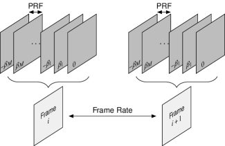
Fig. 1: Sketch of the acquisition schemes deployed for the different pw imaging configurations considered. To form a single frame, a sequence of echo-signals from differently steered PWs is acquired at a prf of $9\text{\,}\mathrm{kHz}\text{/}$. The number of PWs composing each acquisition sequence depends on the imaging configuration (Table 2). The resulting frame rate is determined by the time interval between consecutive acquisition sequences, and is limited by the duration of a single acquisition sequence.

Each PW acquisition was reconstructed using the DAS algorithm detailed in Section 2.2. Coherent compounding of images reconstructed from steered acquisitions was realized by simple pixel-wise averaging. Note that as cpwc-1 only relies on single-PW acquisitions, it is not a compounding method. Its designation was adopted to simplify the naming convention. Also, images obtained from cpwc-1 are identical to input images of the CNN-based image reconstruction (Section 2.2), as the same DAS algorithm was deployed in both cases.

2.4 Speckle Tracking Algorithm

The proposed speckle tracking algorithm is a block-matching algorithm based on normalized cross-correlation. It is heavily inspired by both the speckle tracking method described in [29], which won the challenge on synthetic aperture vector flow imaging (SA-VFI) organized during the 2018 IEEE International Ultrasonic Symposium (IUS) [30], and the PIVlab toolbox [31], a popular software for particle image velocimetry (PIV). Speckle tracking is fundamentally linked to PIV. However, instead of tracking particles to visualize flows, speckle tracking estimates displacements by tracking speckle patterns arising from interferences by scatterers separated by sub-resolution distances, assuming that these patterns are highly correlated between consecutive frames.

To estimate the 2-D displacement field between two consecutive frames $\bm{S}_{1}$ and $\bm{S}_{2}$, both frames were identically subdivided into overlapping interrogation windows. The most probable displacement that occurred between a pair of interrogation windows was obtained by finding the maximum value (peak) of the (2-D) zero-normalized cross-correlation (ZNCC). To achieve sub-pixel precision, we applied a 2-D Gaussian regression around the ZNCC peak, as proposed in [32]. In order to analyze complex displacements, including shear and rotation, this process was deployed in a coarse-to-fine multi-pass algorithm [31]. Between each pass, $\bm{S}_{2}$ was deformed (B-spline interpolation) using the estimated displacements to resemble $\bm{S}_{1}$ more closely. For the next pass, the displacements between $\bm{S}_{1}$ and the deformed $\bm{S}_{2}$ were estimated in a similar way. The remaining displacement estimates of each pass were accumulated, resulting in more accurate estimates after a few passes. After each pass, statistical outliers of the estimates were smoothed using the unsupervised smoothing algorithm described in [33].

Speckle tracking was performed on envelope images, obtained by computing the (pixel-wise) modulus of IQ images. Envelope images were downsampled by a factor of two in the axial dimension, in a uniformly spaced spatial grid of $\lambda{}/4\times{}\lambda{}/4$ (i.e. $596\text{\times}800$ pixels). While applying normalized cross-correlation-based speckle tracking directly to RF signals may lead to a higher precision than using envelope signals [34], especially when analyzing very small displacements close to the Cramér-Rao lower bound [35], it is also much more prone to faulty displacement estimation because of speckle decorrelation [36, Sec. 14.2.1]. Speckle decorrelation increases when analyzing larger displacements, more complex displacements patterns with strong gradients (e.g. rotation), and tissue deformation [37, 38]. As our method is designed to be a robust displacement estimator over a wide range of displacements and flow patterns, envelope images were preferred for the purpose of speckle tracking. However, it is easily adapted to work with RF images if the potential increase in precision for small displacements is of interest.

For adapting the speckle tracking parameters to the imaging configurations and displacement ranges considered, we cross-validated a wide range of different interrogation window sizes, number of passes, and window overlaps using a dedicated numerical test phantom, namely a rotating cylinder centered at the elevation focus of the transducer, similar to the ones deployed in the numerical experiment (Section 3.1). Two different angular velocities were considered, resulting in the same inter-frame displacements considered in this work. Consecutive frames were generated by simulating high-quality images using cpwc-87 without rotating the cylinder between successive steered PW acquisitions (only achievable in a simulation environment). This strategy of “pausing” motion during a complete compounded acquisition sequence was exclusively deployed for the purpose of finding optimal speckle tracking parameters, to avoid being biased by potential motion artifacts. Inter-acquisition motion was considered in the following numerical experiment (Section 3.1).

Interestingly, the speckle tracking parameters yielding best overall displacement estimates in our settings were identical to the ones deployed in [29]. Thus, for all experiments conducted in this work, irrespectively of the displacement range and frame rate under consideration, we deployed the proposed speckle algorithm with four passes, square interrogation windows of $4\text{\,}\mathrm{mm}\text{/}2.5\text{\,}\mathrm{mm}\text{/}2\text{\,}\mathrm{mm}\text{/}1.5\text{\,}\mathrm{mm}\text{/}$, and a window overlap of $65\text{\,}\mathrm{\char 37\relax}\text{/}$.

2.5 Metrics

To evaluate the accuracy of displacement estimates throughout the experiments, we relied on the relative epe (REPE), a normalized version of the well-known endpoint error (EPE), commonly used in flow estimation techniques [39, 40]. Considering a displacement estimate vector $\hat{\bm{u}}\in\mathbb{R}^{2}$ and its true counterpart $\bm{u}\in\mathbb{R}^{2}$, the REPE can be expressed as

$$\text{\glsxtrshort{repe}}=\frac{\lVert\hat{\bm{u}}-\bm{u}\rVert_{2}}{\lVert\bm{u}\rVert_{2}},$$ (4)

where $\lVert\,\cdot\,\rVert_{2}$ represents the Euclidean norm. The main advantage of REPE over EPE comes from its relative nature, enabling a more reliable comparison over a wide range of displacements. On the other hand, REPE becomes unstable as the reference displacement tends to zero. Such cases should therefore be analyzed with care.

We also relied on the mean repe (MREPE) as a global metric to assess a set of $l$ displacement estimates and true counterparts $\{\{\hat{\bm{u}}_{1},\bm{u}_{1}\},\dots,\{\hat{\bm{u}}_{l},\bm{u}_{l}\}\}$ (e.g. extracted from a region of interest), by simply computing the sample mean of all REPE values over the set.

3 Experiments

We conducted two experiments (numerical and in vivo) to assess the performance of the proposed 2-D displacement estimation approach, which combines our CNN-based image reconstruction method [17] (Section 2.2) to reconstruct consecutive frames from single-PW acquisitions and the deployed speckle tracking algorithm (Section 2.4). In both experiments, we compared the proposed CNN-based displacement estimation method to CPWC-based tracking, which consists of applying the same speckle tracking algorithm to consecutive frames reconstructed using conventional CPWC (Section 2.3). For CPWC, a larger number of compounded acquisitions results, if motion artifacts are negligible, in better image quality and consequently in improved displacement estimation, at the cost of a reduced achievable frame rate. Thus, by studying different numbers of compounded acquisitions (Table 2) we compared the proposed approach to multiple levels of displacement estimation accuracy.

3.1 Numerical Experiment

For the first experiment, we used computer simulations to control the motion pattern, the relative echogenicities of tissue-mimicking structures, and the diffraction artifact levels precisely. The goal is to evaluate the quality of displacement tracking that can be achieved using the proposed method in rapidly moving, highly heterogeneous tissue, where strong diffraction artifacts hinder proper motion analysis with conventional CPWC-based tracking. All simulations were conducted using the same SIR simulator used to generate the training dataset (Section 2.2).

We designed a dynamic numerical test phantom composed of scatterers randomly positioned within four cylinders [A, B, C, and D in Fig. 2], embedded in an anechoic background. Each cylinder has a radius of $6.86\text{\,}\mathrm{mm}\text{/}$ and a height of $1.0\text{\,}\mathrm{mm}\text{/}$, the latter corresponding to the resolution cell size in elevation evaluated for the imaging configuration considered [17]. Within each of the four zones, an average of ten scatterers per resolution cell was used to ensure fully developed speckle patterns in the resulting images [41, Sec. 8.4.4]. The cylinders were centered such that cylinder A spawns distinct and spatially separable diffraction artifacts onto cylinders B, C, and D. Cylinders B, C, and D were positioned such that they are maximally covered by EW, SL, and GL artifacts, respectively [Fig. 2]. The mean amplitudes of scatterers located within cylinders B, C, and D were chosen to blend in with the amplitude of EW, SL, and GL artifacts arising from cylinder A [Fig. 2]. Specifically, the mean amplitudes in cylinders A, B, C, and D were set to $20\text{\,}\mathrm{dB}\text{/}$, $-20\text{\,}\mathrm{dB}\text{/}$, $-20\text{\,}\mathrm{dB}\text{/}$, and $0\text{\,}\mathrm{dB}\text{/}$ with respect to an arbitrary $0\text{\,}\mathrm{dB}\text{/}$ reference, respectively. Between successive simulated transmit-receive events (i.e. steered PWs), the scatterers were rotated with a constant counter-clockwise angular velocity around the center of the cylinder within which they are positioned. The same angular velocity was used for all cylinders.

This experiment is designed to evaluate the accuracy of displacement estimates, obtained using the same speckle tracking algorithm on consecutive frames reconstructed with the different image reconstruction methods considered. For this purpose, displacements were estimated using the proposed CNN-based approach, as well as cpwc-1, cpwc-3, cpwc-9, and cpwc-15. Each method was deployed at its maximum achievable frame rate (Table 2), while always considering the same range of inter-frame displacements for comparison purposes. Inter-frame displacements ranging from $3.3\text{\,}\mathrm{\SIUnitSymbolMicro m}\text{/}600\text{\,}\mathrm{\SIUnitSymbolMicro m}\text{/}$ (i.e. approximately from $\lambda/10$ to $2\lambda$) were analyzed, covering a range from the small displacements that typically occur in shear-wave elastography [3] or acoustic radiation force imaging [42], up to the large displacements that typically occur in external compression-based elastography [42]. It can be noted that these inter-frame displacement ranges correspond to velocities up to $5.4\text{\,}\mathrm{m}\text{/}\mathrm{s}$ for the two methods capable of achieving a frame rate of $9\text{\,}\mathrm{kHz}\text{/}$ in these settings (i.e. cpwc-1 and CNN). Such velocities are close to peak velocities inside the cardiovascular system [43].

Two different sets of numerical phantoms were simulated for each image reconstruction method considered and associated frame rate, covering two inter-frame displacement ranges, namely $3.3\text{\,}\mathrm{\SIUnitSymbolMicro m}\text{/}60\text{\,}\mathrm{\SIUnitSymbolMicro m}\text{/}$ (small displacement range) and $33\text{\,}\mathrm{\SIUnitSymbolMicro m}\text{/}600\text{\,}\mathrm{\SIUnitSymbolMicro m}\text{/}$ (large displacement range). The respective angular velocities were determined such that the maximum inter-frame displacement occurs at a radius of $6.5\text{\,}\mathrm{mm}\text{/}$. The remaining border of $0.36\text{\,}\mathrm{mm}\text{/}$ was ignored to avoid speckle tracking border effects in the quality evaluation. It corresponds to the approximate average resolution cell size in the transducer plane. A similar zone was ignored in the center of each cylinder. Displacement ranges are made explicit in Table 3 for each image reconstruction method considered, and the corresponding cross-radial velocity ranges are also provided as additional information. It can be noted that the large-displacement case involves displacements greater than half the deployed wavelength. As a result, motion artifacts are expected for CPWC methods [13].

TABLE 3: Displacement and Velocity Ranges Considered
for the Numerical Experiment

Method	Frame	Large Ranges		Small Ranges
	Rate	D. ($\mathrm{\SIUnitSymbolMicro m}\text{/}$)	V. ($\mathrm{cm}\text{/}\mathrm{s}$)	D. ($\mathrm{\SIUnitSymbolMicro m}\text{/}$)	V. ($\mathrm{cm}\text{/}\mathrm{s}$)
cnn	$9\text{\,}\mathrm{kHz}\text{/}$	$33600$	$29.7540$	$3.360$	2.97–54.
cpwc-1	$9\text{\,}\mathrm{kHz}\text{/}$	$33600$	$29.7540$	$3.360$	2.97–54.
cpwc-3	$3\text{\,}\mathrm{kHz}\text{/}$	$33600$	09.9–180	$3.360$	0.99–18.
cpwc-9	$1\text{\,}\mathrm{kHz}\text{/}$	$33600$	$3.360$	$3.360$	0.33–60.
cpwc-15	$0.6\text{\,}\mathrm{kHz}\text{/}$	$33600$	$2.036$	$3.360$	$0.203.6$

For all test configurations considered (i.e. method and displacement range), $50$ statistically independent scatterer realizations were simulated, resulting in $50$ inter-frame displacement estimate maps for each configuration. The accuracy of each method was measured locally in terms of REPE, by computing 4 for each displacement estimate (grid point) and corresponding true (analytical) value. The average local REPE was also computed over the $50$ independent realizations (in each displacement estimate grid point).

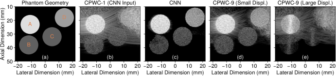
Fig. 2: B-mode image representations ($80$-$\mathrm{dB}\text{/}$ range) of a numerical test phantom sample: 2 the 2-D geometry of the deployed numerical phantoms, composed of four cylinders (A, B, C, and D) filled with dense point-scatterers rotating at constant angular velocity around their respective cylinder center; 2 image reconstructed by das beamforming a single plane-wave (pw) acquisition (cpwc-1), simultaneously representing the cnn input image for the proposed method; 2 image reconstructed using CNN-based reconstruction; images reconstructed by cpwc using nine steered PW acquisitions (cpwc-9): 2 small displacement range and 2 large displacement range. The frame rate and displacement range for each image reconstruction method considered are given in Table 3.

3.2 In Vivo Experiment

For the second experiment, we applied the proposed approach to in vivo acquisitions, to analyze the natural tissue motion around the carotid artery. The goal of this experiment is to evaluate the robustness and translatability of the results obtained in the numerical experiment to the full complexity of in vivo imaging. As the natural tissue motion induced by cardiac pulsations in the vicinity of the carotid artery is small compared with the one considered in the numerical experiment, similar inter-frame displacements could be studied at a much lower frame rate, enabling the use of cpwc-87 for obtaining high-quality reference displacement estimates.

We analyzed the slow-moving tissue between the skin and the carotid artery of a healthy volunteer. In particular, motion within a specific tissue region of size $5\text{\times}5\text{\,}\mathrm{mm}\text{/}$ (Fig. 4) was analyzed from consecutive frames acquired at a frame rate of $10\text{\,}\mathrm{Hz}\text{/}$. This resulted in inter-frame displacements similar to those studied in the numerical experiment (Section 3.1), namely ranging from $5\text{\,}\mathrm{\SIUnitSymbolMicro m}\text{/}125\text{\,}\mathrm{\SIUnitSymbolMicro m}\text{/}$ approximately [Fig. 4]. Therefore, identical speckle tracking settings were used (Section 2.4). Speckle tracking was performed on full images, but we restricted our analysis to a specific zone characterized by fully developed speckle patterns, plagued by diffraction artifacts mainly originating from the highly echogenic carotid walls when imaged using cpwc-1 [Fig. 4]. The mean echogenicity of the analyzed speckle zone was approximately $20\text{\,}\mathrm{dB}\text{/}$ lower than the echogenicity of the carotid walls, thus similar to the relative echogenicity between cylinders A and D studied in the numerical experiment.

We compared displacement estimates obtained using the proposed CNN-based approach, cpwc-1 (i.e. the CNN input), and cpwc-15 with respect to reference displacement estimates obtained with cpwc-87 (Table 2). As compounded acquisition sequences were performed at a PRF of $9\text{\,}\mathrm{kHz}\text{/}$, motion artifacts were negligible. More specifically, the maximum mean displacement estimated during a complete compounded acquisition sequence for cpwc-87 was approximately of $12\text{\,}\mathrm{\SIUnitSymbolMicro m}\text{/}$. This amounts to approximately $\lambda/25$ and motion artifacts can therefore be neglected [13]. For each method being compared, consecutive frames were reconstructed using the relevant subset of steered PW (s) acquired for the reference cpwc-87 method (Section 2.3).

A total of $30$ frames were obtained at a frame rate of $10\text{\,}\mathrm{Hz}\text{/}$, resulting in $29$ inter-frame displacement estimate maps. For each inter-frame displacement estimate map, the accuracy of each method was measured locally in terms of REPE, by computing 4 for each displacement estimate (grid point) and corresponding reference value (cpwc-87). The quality of the displacement estimates for each pair of frames was assessed by computing the MREPE obtained within the region of interest.

4 Results

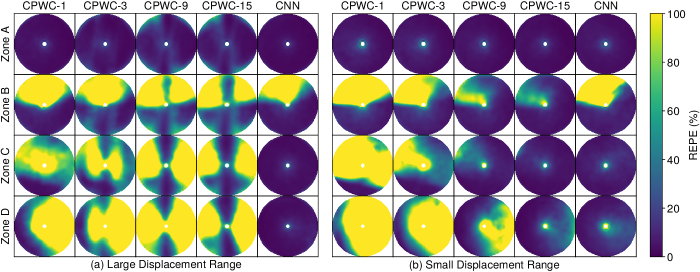
Fig. 3: Local repe, averaged over $50$ independent realizations, of the 2-D displacement estimates inside each of the numerical phantom zones [A, B, C, and D in Fig. 2], obtained by applying the deployed 2-D speckle tracking algorithm (Section 2.4) on two consecutive frames for the two inter-frame displacement ranges considered: 3 large displacement range (from $33\text{\,}\mathrm{\SIUnitSymbolMicro m}\text{/}600\text{\,}\mathrm{\SIUnitSymbolMicro m}\text{/}$); 3 small displacement range (from $3.3\text{\,}\mathrm{\SIUnitSymbolMicro m}\text{/}60\text{\,}\mathrm{\SIUnitSymbolMicro m}\text{/}$). Consecutive frames were reconstructed either by cpwc from $13915$ differently steered PWs, or using the proposed cnn-based image reconstruction method from single PWs. The frame rate and displacement range for each image reconstruction method considered are given in Table 3. The displayed repe range is limited to $100\text{\,}\mathrm{\char 37\relax}\text{/}$. Local repe values were interpolated onto a fine grid for display purposes.

TABLE 4: Global Evaluation Metrics of the Numerical Experiment

Zone	Metric	Large Displacement Range					Small Displacement Range
		cpwc-1	cpwc-3	cpwc-9	cpwc-15	cnn	cpwc-1	cpwc-3	cpwc-9	cpwc-15	cnn
A	RVE ($\mathrm{\char 37\relax}\text{/}$)	$100.0000$	$100.0000$	$100.0000$	$100.0000$	$100.0000$	$100.0000$	$100.0000$	$100.0000$	$100.0000$	$100.0000$
	mrepe ($\mathrm{\char 37\relax}\text{/}$)	$4.4460$	$7.2406$	$12.9919$	$12.8443$	$3.6159$	$7.3442$	$6.9130$	$5.2454$	$4.3558$	$5.8100$
B	RVE ($\mathrm{\char 37\relax}\text{/}$)	$63.1038$	$69.4758$	$63.1038$	$68.8592$	$74.6146$	$57.7595$	$73.7924$	$99.3834$	$99.6917$	$67.4203$
	mrepe ($\mathrm{\char 37\relax}\text{/}$)	$78.5797$	$61.3176$	$82.7172$	$72.6517$	$48.3588$	$143.9140$	$64.3007$	$26.6593$	$19.3666$	$95.4429$
C	RVE ($\mathrm{\char 37\relax}\text{/}$)	$85.2697$	$77.8008$	$51.5560$	$65.2490$	$100.0000$	$29.2531$	$81.6390$	$100.0000$	$100.0000$	$100.0000$
	mrepe ($\mathrm{\char 37\relax}\text{/}$)	$67.5022$	$66.2965$	$91.4927$	$71.0270$	$4.9836$	$192.5744$	$54.3719$	$17.6430$	$8.2927$	$9.6123$
D	RVE ($\mathrm{\char 37\relax}\text{/}$)	$44.5932$	$44.1813$	$34.8095$	$49.4336$	$100.0000$	$22.1421$	$42.0185$	$82.2863$	$99.6910$	$99.5881$
	mrepe ($\mathrm{\char 37\relax}\text{/}$)	$135.1803$	$120.6853$	$123.7411$	$100.1869$	$5.5143$	$504.3849$	$159.1545$	$52.8969$	$17.8259$	$15.6713$

4.1 Numerical Experiment

Fig. 3 displays local REPE values, averaged over the $50$ independent realizations performed in each configuration considered (Section 3.1). To support the analysis, we also provide two global metrics computed for each zone, method, and displacement range considered (Table 4), namely the MREPE and the ratio of valid estimates (RVE). For the RVE, a local REPE value (averaged over the $50$ independent realizations) exceeding $100\text{\,}\mathrm{\char 37\relax}\text{/}$ was deemed invalid. It is thus directly related to the amount of saturated REPE values depicted in Fig. 3, and provides a global metric less sensitive than MREPE to potentially huge-but-scarce local REPE values.
Zone A was designed such that it did not suffer from diffraction artifacts and could be used to assess displacement estimation in pure speckle zones. In the large-displacement case [Fig. 3], CPWC-based tracking suffered from increasing motion artifacts with the number of compounded acquisitions when tracking identical inter-frame displacements (i.e. at decreasing frame rates), reaching a stable motion artifact level after nine compounded acquisitions. The proposed method performed best and improved over cpwc-1 both in terms of local and global metrics. In the small-displacement case [Fig. 3], motion artifacts are negligible and all methods performed efficiently. A typical comparison of CPWC with and without motion artifacts is shown in Fig. 2 and 2 for cpwc-9.

Zone B was designed to suffer from EW artifacts. The proposed method was not capable of restoring speckle patterns shadowed by EW artifacts accurately, resulting in performance metrics only slightly improved compared with cpwc-1. Inaccurate restoration of speckle patterns plagued by EW artifacts can be observed in Fig. 2 (e.g. clipped values). These artifacts could only be progressively resolved in the small displacement case [Fig. 3] with the increase in compounded acquisitions, because motion artifacts are negligible in that case.

Zone C was designed to suffer from SL artifacts. In the large-displacement case [Fig. 3], the reduction in SL artifacts achieved by compounding several acquisitions was counteracted by the induced motion artifacts, except in zones of pure lateral movement, making proper tracking impossible using CPWC-based tracking. The proposed method was capable of properly estimating displacements, with a quality only slightly worse than in artifact-free zone A. In the small-displacement case [Fig. 3], CPWC-based tracking was improved with the increase in compounded acquisitions, thanks to a more efficient SL reduction than with motion artifacts. The proposed method achieved a quality slightly worse than cpwc-15 but significantly better than cpwc-9.

Zone D was designed to suffer from GL artifacts, that increase in strength towards the right edge of the image. In the large-displacement case [Fig. 3], compounding multiple acquisitions reduced GL artifacts. Yet, motion artifacts prevented accurate displacement estimation except in zones of pure lateral movement. The proposed method significantly improved the displacement estimation quality over cpwc-1 and was the only method to enable tracking displacements in this case. In the small-displacement case [Fig. 3], the increase in compounded acquisitions enabled CPWC-based tracking to reduce the effect of GLs and restore the underlying speckle patterns, progressively resulting in an increased RVE and lower MREPE. The proposed method performed slightly better than cpwc-15.

4.2 In Vivo Experiment

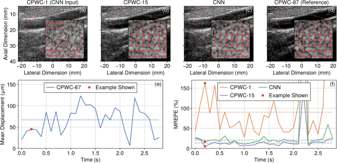
Fig. 4: Examples of displacement estimates, mean reference displacement magnitude, and mrepe, obtained using the displacement estimation methods considered, in a fully developed speckle zone above the carotid artery: images of a longitudinal view of the carotid artery, are shown for 4 cpwc-1 (also CNN input), 4 cpwc-15, 4 CNN, and 4 cpwc-87 (reference); the bottom row shows 4 the mean reference displacement magnitude and 4 the mrepe along the entire in vivo sequence for each method considered. In each B-mode image of the top row, the square region of interest is highlighted and the corresponding magnified inset displays the 2-D displacement estimates. B-mode images are displayed using a dynamic range of $50\text{\,}\mathrm{dB}\text{/}$. The mean value (through time) of each quantity represented by a colorized solid line in 4 and 4 is represented by a horizontal dashed line of the same color. These mean values were computed ignoring samples at $2.2\text{\,}\mathrm{s}\text{/}$ due to the resulting extreme mrepe values. An animation of the figure and the corresponding slideshow are provided as supplementary material.

From the example images and corresponding displacement estimates [Fig. 4, 4, 4 and 4], one can observe that cpwc-1 suffered from diffraction artifacts (mainly caused by GLs and SLs arising from the carotid walls), disturbing both the speckle patterns and the resulting displacement estimates. These artifacts were strongly reduced using cpwc-15, leading to speckle patterns similar to the reference ones (cpwc-87), resulting in accurate displacement estimates. The proposed CNN-based imaging approach also reduced these artifacts, restoring the underlying speckle patterns accurately. This resulted in local displacement estimates with a quality similar to that obtained with cpwc-15.

The analysis of the MREPE values over time [Fig. 4] shows that, while cpwc-1 was generally unable to estimate inter-frame motion properly, the proposed method resulted in high and stable displacement estimation quality, similar to (though slightly worse than) cpwc-15. This observation matches the results of the numerical experiments on small displacements (Section 4.1). At $2.2\text{\,}\mathrm{s}\text{/}$, significant deviations in the MREPE values for all methods compared can be observed [Fig. 4]. As the estimated reference tissue displacement at this time instant is very small ($\sim{}5\text{\,}\mathrm{\SIUnitSymbolMicro m}\text{/}$) [Fig. 4], local REPE values, and as a consequence MREPE values, can be very sensitive to small absolute errors. Moreover, it is likely that such small displacements are close to the minimum achievable displacement estimation error (Cramér-Rao lower bound), thus over amplifying the inherent sensitivity of the REPE to very small reference displacements. This behavior can also be observed in the numerical experiment on small displacements towards the center of rotation of zones C and D [Fig. 3]. Therefore, all values estimated at $2.2\text{\,}\mathrm{s}\text{/}$ were ignored in the computation of the following global metrics. As global metrics, we computed the mean value through time (ignoring said time instant) of each estimated quantity [represented as dashed lines in Fig. 4 and 4]. The estimated mean inter-frame displacement is $66.83\text{\,}\mathrm{\SIUnitSymbolMicro m}\text{/}$. The MREPE values are $90.18\text{\,}\mathrm{\char 37\relax}\text{/}13.38\text{\,}\mathrm{\char 37\relax}\text{/}20.73\text{\,}\mathrm{\char 37\relax}\text{/}$ for cpwc-1, cpwc-15, and the proposed CNN-based method, respectively.

5 Discussion

In this work, we proposed a 2-D motion estimation approach based on single unfocused acquisitions to reconstruct consecutive frames and on pairs of consecutive frames to estimate local displacements. This approach relies on our CNN-based image reconstruction method [17] to reconstruct full-view US frames from single unfocused acquisitions. It consists of first reconstructing low-quality images using a backprojection-inspired DAS algorithm and then feeding them to a CNN, specifically trained to reduce diffraction artifacts inherent to ultrafast US imaging. Inter-frame displacements are estimated by applying a state-of-the-art 2-D speckle tracking algorithm on consecutive frame pairs only.

5.1 Performance in Numerical Conditions

An important observation is that the proposed approach could not estimate displacements accurately in zones dominated by EW artifacts (Fig. 3, zone B). This is directly related to the fact that the CNN deployed is not capable of restoring the underlying speckle patterns accurately [Fig. 2]. Slight improvements were observed compared with conventional single PW imaging (cpwc-1), but far less striking than in zones dominated by SL and GL artifacts (Fig. 3, zones C and D). In [17], we already observed that EW artifacts were the most difficult artifacts to deal with, but also that the restoration quality improved with the increase of the CNN capacity. The latter implies that the reduction of these artifacts might be further improved using a more efficient CNN architecture or training process.

As expected, we observed in the large-displacement case that compounding multiple acquisitions in an attempt to improve the obtained image quality induces strong motion artifacts, mainly due to destructive interferences caused by axial motion. In the presence of motion artifacts, conventional CPWC-based speckle tracking was generally incapable of providing valid displacement estimation, in particular in zones plagued by strong diffraction artifacts. Consequently, compounding multiple acquisitions decreased the displacement estimation quality compared with single-PW acquisitions (cpwc-1). While motion compensation techniques have been proposed to tackle this issue [16], it remains unclear if motion-compensated coherent compounding can be deployed in zones plagued by diffraction artifacts (as it is based on inter-acquisition motion estimation), and if it actually improves displacement estimation quality in artifact-free zones compared with single unfocused acquisitions. We demonstrated that the proposed single PW CNN-based approach is capable of providing high-quality displacement estimates in artifact-free zones, as well as in zones plagued by SL and GL artifacts.

In the case of small displacements, increasing the number of compounded acquisitions using CPWC-based tracking progressively increased, as expected, the accuracy of displacement estimation. The proposed CNN-based approach achieves a displacement estimation quality comparable to cpwc-15 in zones suffering from SL and GL artifacts and comparable to cpwc-9 in artifact-free zones. It can be noted that the relative estimation precision achieved by the proposed approach was generally worse when analyzing small inter-frame displacements than in larger displacement cases. This was also observed for conventional CPWC-based tracking in artifact-free zones [e.g. compare cpwc-1, zone A in Fig. 3 and 3]. This mainly comes from the fact that the minimum estimation error of correlation-based tracking converges to a minimum value (Cramér-Rao lower bound), which, relatively speaking, becomes more significant for smaller displacements [42]. For quantifying very small displacements, applying speckle tracking to RF data instead of envelope data may improve precision [34], [36, Sec. 14.2.1], at the expense of a reduced robustness to speckle decorrelation.

5.2 Performance in Physical Conditions

We demonstrated that the proposed CNN-based approach, which relies on single-PW acquisitions, significantly improved over conventional single PW imaging (cpwc-1). It also achieved an accuracy of inter-frame displacement estimation similar to that of $15$ compounded acquisitions (cpwc-15), in conditions where motion artifacts were negligible and thus did not limit the performance of the comparative cpwc-15 method.

Overall, the quantitative evaluations performed in the in vivo experiment are comparable to those of the numerical one. This does not only show that the proposed method can be applied to in vivo data successfully, even though the CNN used for image reconstruction was trained on simulated data only, it also suggests that the results of the numerical experiments are robust and translatable (to some extent) to experimental conditions. More specifically, as motion artifacts were negligible in the in vivo experiment, the results obtained are best compared with the ones obtained in the numerical experiment on small displacements [Fig. 3]. It can be noted that the artifacts initially shadowing the zone in which displacement estimates were analyzed seem to be a combination of GL and SL artifacts spawned by the highly echogenic carotid walls [Fig. 4]. Thus, zones C and D of the numerical experiment are of interest for comparison purposes, as they contain SL and GL artifacts, respectively [Fig. 2]. While the quantitative metrics are similar, it is important to note that this presumptive combination of GL and SL artifacts was not present in the numerical experiment, and that the “signal-to-artifact” ratio was probably more favorable in the in vivo experiment than in the numerical one. One can observe that cpwc-15 performed better than the proposed method in the in vivo experiment [Fig. 4], whereas both methods performed similarly well in zones C and D of the numerical experiment on small displacements (Table 4). A performance drop of the proposed approach from numerical to physical conditions was expected since the deployed CNN was trained on simulated images only. This performance drop was already observed in [17], in which a detailed discussion on the discrepancies between the numerical and physical conditions can be found.

It should be noted that the in vivo experiment was intentionally carried out on a slow moving tissue zone. This enabled us to obtain reference displacement estimates for quantitative evaluation purposes, and to select a frame rate, identical for all methods considered, resulting in inter-frame displacements within ranges of interest. However, as speckle tracking is agnostic to the underlying frame rate, the results are fully translatable to fast motion cases with similar inter-frame displacement ranges, provided that the required frame rate is achievable by the method deployed.

5.3 Potential, Perspectives, and Limitations

The proposed approach is overall able to provide high-quality estimates for a wide range of 2-D inter-frame displacements, even in tissue regions dominated by SL and GL artifacts. As it only relies on single unfocused acquisitions to reconstruct consecutive frames, it is immune to motion artifacts. Moreover, it is limited only by the propagation time of acoustic waves, making it especially interesting for the analysis of rapidly changing events at very high frames rates, such as the propagation of shear waves in tissue or complex flow patterns within the cardiovascular system, where displacement estimation techniques based on multi-acquisition image reconstruction methods may not be deployable.

The major limitation is that the current implementation of the proposed approach was not able to provide accurate displacement estimates in regions dominated by EW artifacts. This is most probably due to the fact that the patterns resulting from EW artifacts resemble speckle patterns much more closely than the ones resulting from SL and GL artifacts [Fig. 2]. Since CNNs are, in essence, based on pattern recognition, the close resemblance of two patterns, one sought to be removed, the other to be preserved, represents a greater difficulty compared with a situation in which the two patterns are very distinctive. Both the EW behavior and the general performance of the approach might be further improved by augmenting the performance of the CNN used for image reconstruction. For instance, the use of a higher-capacity CNN or a more efficient training process may improve the restoration of tissue structures hidden by EW artifacts. Another way to tackle this limitation would be to use transmit apodization [22]. This technique can significantly reduce EW artifacts, at the cost of limited energy towards the image borders. However, its effectiveness is limited by the apodization capability of US systems, in particular by the transmitter complexity. If the method is not used at maximum achievable frame rate, and in the presence of sufficiently stationary motion, the robustness and precision of the displacement estimation could be improved, for instance, by averaging multiple displacement estimates or by using ensemble correlation [29].

This study was limited to tracking fully developed speckle patterns, hence no insights about tracking tissue structures arising from specular or diffractive scattering should be drawn from it directly. Yet, carotid wall movement was observed to be similar to that of conventional methods (see animation of Fig. 4, supplementary material). The training set was also limited to simulated images of fully developed speckle zones resulting from diffusive scattering. In [17], we observed that, while reconstructing other tissue structures is generally possible, the performance may be less potent than in fully developed speckle zones. Using a versatile training set may be considered to widen the applicability of both the reconstruction approach and the displacement tracking method proposed here.

On a more general perspective, this work further validates the potency of the CNN-based image reconstruction method introduced in [17]. Indeed, this method not only provides high-quality images from single unfocused acquisitions, but also preserves the information of underlying physical phenomena that can be further exploited for estimating inter-frame displacements accurately.

6 Conclusion

In this work we proposed an approach for estimating 2-D inter-frame displacements in the context of ultrafast US imaging. The approach consists of a CNN trained to restore high-quality images from single unfocused acquisitions and a speckle tracking algorithm to estimate inter-frame displacements from two consecutive frames only. Compared with conventional multi-acquisition strategies, this approach is immune to motion artifacts and enables accurate motion estimation at maximum frames rates, even in highly heterogeneous tissues prone to strong diffraction artifacts. Numerical and in vivo results demonstrated that the proposed approach is capable of estimating displacement vector fields from single-PW acquisitions accurately, including in zones initially hidden by SL and GL artifacts. The proposed approach may thus unlock the full potential of ultrafast US, with direct applications to imaging modes that depend on accurate motion estimation at maximum frame rates, such as shear-wave elastography or ultrasensitive echocardiography.

References

- [1] M. Tanter and M. Fink, “Ultrafast imaging in biomedical ultrasound,” IEEE Trans. Ultrason., Ferroelectr., Freq. Control, vol. 61, no. 1, pp. 102–119, Jan. 2014.
- [2] J. Bercoff, M. Tanter, and M. Fink, “Supersonic shear imaging: a new technique for soft tissue elasticity mapping,” IEEE Trans. Ultrason., Ferroelectr., Freq. Control, vol. 51, no. 4, pp. 396–409, Apr. 2004.
- [3] G. Montaldo, M. Tanter, J. Bercoff, N. Benech, and M. Fink, “Coherent plane-wave compounding for very high frame rate ultrasonography and transient elastography,” IEEE Trans. Ultrason., Ferroelectr., Freq. Control, vol. 56, no. 3, pp. 489–506, Mar. 2009.
- [4] P. Santos et al., “Natural shear wave imaging in the human heart: Normal values, feasibility, and reproducibility,” IEEE Trans. Ultrason., Ferroelectr., Freq. Control, vol. 66, no. 3, pp. 442–452, Mar. 2019.
- [5] C. Papadacci, M. Pernot, M. Couade, M. Fink, and M. Tanter, “High-contrast ultrafast imaging of the heart,” IEEE Trans. Ultrason., Ferroelectr., Freq. Control, vol. 61, no. 2, pp. 288–301, Feb. 2014.
- [6] M. Pernot, M. Couade, P. Mateo, B. Crozatier, R. Fischmeister, and M. Tanter, “Real-time assessment of myocardial contractility using shear wave imaging,” J. Am. Coll. Cardiol., vol. 58, no. 1, pp. 65–72, Jun. 2011.
- [7] H. Geyer et al., “Assessment of myocardial mechanics using speckle tracking echocardiography: Fundamentals and clinical applications,” J. Am. Soc. Echocardiogr., vol. 23, no. 4, pp. 351–369, Apr. 2010.
- [8] M. Cikes, L. Tong, G. R. Sutherland, and J. D’hooge, “Ultrafast cardiac ultrasound imaging,” JACC Cardiovasc. Imaging, vol. 7, no. 8, pp. 812–823, Aug. 2014.
- [9] J.-U. Voigt et al., “Definitions for a common standard for 2D speckle tracking echocardiography: consensus document of the EACVI/ASE/Industry task force to standardize deformation imaging,” Eur. Hear. J. - Cardiovasc. Imaging, vol. 16, no. 1, pp. 1–11, Jan. 2015.
- [10] J. Bercoff et al., “Ultrafast compound doppler imaging: providing full blood flow characterization,” IEEE Trans. Ultrason., Ferroelectr., Freq. Control, vol. 58, no. 1, pp. 134–147, Jan. 2011.
- [11] E. Macé, G. Montaldo, I. Cohen, M. Baulac, M. Fink, and M. Tanter, “Functional ultrasound imaging of the brain,” Nat. Methods, vol. 8, no. 8, pp. 662–664, Aug. 2011.
- [12] J. Cheng and J.-Y. Lu, “Extended high-frame rate imaging method with limited-diffraction beams,” IEEE Trans. Ultrason., Ferroelectr., Freq. Control, vol. 53, no. 5, pp. 880–899, May 2006.
- [13] B. Denarie et al., “Coherent plane wave compounding for very high frame rate ultrasonography of rapidly moving targets,” IEEE Trans. Med. Imaging, vol. 32, no. 7, pp. 1265–1276, Jul. 2013.
- [14] J. Porée, D. Posada, A. Hodzic, F. Tournoux, G. Cloutier, and D. Garcia, “High-frame-rate echocardiography using coherent compounding with doppler-based motion-compensation,” IEEE Trans. Med. Imaging, vol. 35, no. 7, pp. 1647–1657, Jul. 2016.
- [15] J. Porée, D. Garcia, B. Chayer, J. Ohayon, and G. Cloutier, “Noninvasive vascular elastography with plane strain incompressibility assumption using ultrafast coherent compound plane wave imaging,” IEEE Trans. Med. Imaging, vol. 34, no. 12, pp. 2618–2631, Dec. 2015.
- [16] P. Joos et al., “High-frame-rate speckle-tracking echocardiography,” IEEE Trans. Ultrason., Ferroelectr., Freq. Control, vol. 65, no. 5, pp. 720–728, May 2018.
- [17] D. Perdios, M. Vonlanthen, F. Martinez, M. Arditi, and J.-P. Thiran, “CNN-based image reconstruction method for ultrafast ultrasound imaging,” Aug. 2020. [Online]. Available: https://arxiv.org/abs/2008.12750
- [18] ——, “Deep learning based ultrasound image reconstruction method: A time coherence study,” in 2019 IEEE Int. Ultrason. Symp., Oct. 2019, pp. 448–451.
- [19] J. A. Jensen, S. I. Nikolov, A. C. H. Yu, and D. Garcia, “Ultrasound vector flow imaging—Part II: Parallel systems,” IEEE Trans. Ultrason., Ferroelectr., Freq. Control, vol. 63, no. 11, pp. 1722–1732, Nov. 2016.
- [20] S. Fadnes, S. A. Nyrnes, H. Torp, and L. Lovstakken, “Shunt flow evaluation in congenital heart disease based on two-dimensional speckle tracking,” Ultrasound Med. Biol., vol. 40, no. 10, pp. 2379–2391, Oct. 2014.
- [21] M. Tanter, J. Bercoff, L. Sandrin, and M. Fink, “Ultrafast compound imaging for 2-D motion vector estimation: application to transient elastography,” IEEE Trans. Ultrason., Ferroelectr., Freq. Control, vol. 49, no. 10, pp. 1363–1374, Oct. 2002.
- [22] J. Jensen, M. B. Stuart, and J. A. Jensen, “Optimized plane wave imaging for fast and high-quality ultrasound imaging,” IEEE Trans. Ultrason., Ferroelectr., Freq. Control, vol. 63, no. 11, pp. 1922–1934, Nov. 2016.
- [23] J. A. Jensen, “A model for the propagation and scattering of ultrasound in tissue,” J. Acoust. Soc. Am., vol. 89, no. 1, p. 182, Jan. 1991.
- [24] P. Thevenaz, T. Blu, and M. Unser, “Interpolation revisited,” IEEE Trans. Med. Imaging, vol. 19, no. 7, pp. 739–758, Jul. 2000.
- [25] O. Ronneberger, P. Fischer, and T. Brox, “U-Net: Convolutional networks for biomedical image segmentation,” in Med. Image Comput. Comput. Interv. – MICCAI 2015, Nov. 2015, pp. 234–241.
- [26] K. H. Jin, M. T. McCann, E. Froustey, and M. Unser, “Deep convolutional neural network for inverse problems in imaging,” IEEE Trans. Image Process., vol. 26, no. 9, pp. 4509–4522, Sep. 2017.
- [27] D. P. Kingma and J. Ba, “Adam: A method for stochastic optimization,” pp. 1–15, Dec. 2014. [Online]. Available: https://arxiv.org/abs/1412.6980
- [28] J. A. Jensen, “FIELD: A program for simulating ultrasound systems,” in 10th Nord. Conf. Biomed. Imaging, vol. 4, no. Supplement 1, 1996, pp. 351–353.
- [29] V. Perrot and D. Garcia, “Back to basics in ultrasound velocimetry: Tracking speckles by using a standard PIV algorithm,” in 2018 IEEE Int. Ultrason. Symp., Oct. 2018, pp. 206–212.
- [30] J. A. Jensen, H. Liebgott, F. Cervenansky, and C. A. Villagomez Hoyos, “SA-VFI: the IEEE IUS challenge on synthetic aperture vector flow imaging,” in 2018 IEEE Int. Ultrason. Symp., Oct. 2018, pp. 1–5.
- [31] W. Thielicke and E. J. Stamhuis, “PIVlab – towards user-friendly, affordable and accurate digital particle image velocimetry in MATLAB,” J. Open Res. Softw., vol. 2, no. 1, Oct. 2014.
- [32] H. Nobach and M. Honkanen, “Two-dimensional Gaussian regression for sub-pixel displacement estimation in particle image velocimetry or particle position estimation in particle tracking velocimetry,” Exp. Fluids, vol. 38, no. 4, pp. 511–515, Apr. 2005.
- [33] D. Garcia, “Robust smoothing of gridded data in one and higher dimensions with missing values,” Comput. Stat. Data Anal., vol. 54, no. 4, pp. 1167–1178, Apr. 2010.
- [34] W. F. Walker and G. E. Trahey, “A fundamental limit on the performance of correlation based phase correction and flow estimation techniques,” IEEE Trans. Ultrason., Ferroelectr., Freq. Control, vol. 41, no. 5, pp. 644–654, Sep. 1994.
- [35] ——, “A fundamental limit on delay estimation using partially correlated speckle signals,” IEEE Trans. Ultrason., Ferroelectr., Freq. Control, vol. 42, no. 2, pp. 301–308, Mar. 1995.
- [36] C. P. Loizou, C. S. Pattichis, and J. D’hooge, Eds., Handbook of Speckle Filtering and Tracking in Cardiovascular Ultrasound Imaging and Video, ser. Healthcare Technologies. Institution of Engineering and Technology, 2018.
- [37] L. N. Bohs, B. J. Geiman, M. E. Anderson, S. C. Gebhart, and G. E. Trahey, “Speckle tracking for multi-dimensional flow estimation,” Ultrasonics, vol. 38, no. 1-8, pp. 369–375, Mar. 2000.
- [38] J. Meunier and M. Bertrand, “Ultrasonic texture motion analysis: theory and simulation,” IEEE Trans. Med. Imaging, vol. 14, no. 2, pp. 293–300, Jun. 1995.
- [39] M. Otte and H. H. Nagel, “Optical flow estimation: Advances and comparisons,” in Comput. Vis. — ECCV ’94. Springer Berlin Heidelberg, May 1994, pp. 49–60.
- [40] S. Baker, D. Scharstein, J. P. Lewis, S. Roth, M. J. Black, and R. Szeliski, “A database and evaluation methodology for optical flow,” Int. J. Comput. Vis., vol. 92, no. 1, pp. 1–31, Mar. 2011.
- [41] T. L. Szabo, Diagnostic Ultrasound Imaging: Inside Out, 2nd ed., ser. Biomedical Engineering. Academic Press, 2014.
- [42] G. F. Pinton, J. J. Dahl, and G. E. Trahey, “Rapid tracking of small displacements with ultrasound,” IEEE Trans. Ultrason., Ferroelectr., Freq. Control, vol. 53, no. 6, pp. 1103–1117, Jun. 2006.
- [43] H. F. Routh, “Doppler ultrasound,” IEEE Eng. Med. Biol. Mag., vol. 15, no. 6, pp. 31–40, Nov. 1996.