On complexity and convergence of high-order
coordinate descent algorithms for smooth nonconvex box-constrained minimization

Abstract

Coordinate descent methods have considerable impact in global optimization because global (or, at least, almost global) minimization is affordable for low-dimensional problems. Coordinate descent methods with high-order regularized models for smooth nonconvex box-constrained minimization are introduced in this work. High-order stationarity asymptotic convergence and first-order stationarity worst-case evaluation complexity bounds are established. The computer work that is necessary for obtaining first-order $\varepsilon$-stationarity with respect to the variables of each coordinate-descent block is $O(\varepsilon^{-(p+1)/p})$ whereas the computer work for getting first-order $\varepsilon$-stationarity with respect to all the variables simultaneously is $O(\varepsilon^{-(p+1)})$. Numerical examples involving multidimensional scaling problems are presented. The numerical performance of the methods is enhanced by means of coordinate-descent strategies for choosing initial points.

Key words: Coordinate descent methods, bound-constrained minimization, worst-case evaluation complexity.

AMS subject classifications: 90C30, 65K05, 49M37, 90C60, 68Q25.

1 Introduction

In order to minimize a multivariate function it is natural to keep fixed some of the variables and to modify the remaining ones trying to decrease the objective function value. Coordinate descent (CD) methods proceed systematically in this way and, many times, obtain nice approximations to minimizers of practical optimization problems. Wright [58] surveyed traditional approaches and modern advances on the introduction and analysis of CD methods. Although the CD idea is perhaps the most natural one to optimize functions, it received little attention from researchers due to poor performance in many cases and lack of challenges in terms of convergence theory [55]. The situation changed dramatically in the last decades. CD methods proved to be useful for solving machine learning, deep learning and statistical learning problems in which the number of variables is big and the accuracy required at the solution is moderate [18, 52]. Many applications arose and, in present days, efficient implementations and insightful theory for understanding the CD properties are the subject of intense research. See, for example, [2, 3, 15, 16, 17, 20, 30, 36, 47, 60, 61] among many others.

In this paper we are concerned with complexity issues of CD methods that employ high-order models to approximate the subproblems that arise at each iteration. The use of high-order models for unconstrained optimization was defined and analyzed from the point of view of worst-case complexity in [6] and subsequent papers [5, 24, 39, 40, 48, 62]. In [5] numerical implementations with quartic regularization were introduced. In [24], [39], [40], and [48], new high-order regularization methods were introduced with Hölder, instead of Lipschitz, conditions on the highest-order derivatives employed. In [46], high-order methods were studied as discretizations of ordinary differential equations. These methods generalize the methods based on third-order models introduced in [43] and later developed in [22, 23, 33, 35, 53] among many others. Griewank [43] introduced third-order regularization having in mind affine scaling properties. Nesterov and Polyak [53] introduced the first cubic regularized Newton methods with better complexity results than the ones that were known for gradient-like algorithms [41]. In [21], a multilevel strategy that exploits a hierarchy of problems of decreasing dimension was introduced in order to reduce the global cost of the step computation. However, high-order methods remain difficult to implement in the many-variables case due to the necessity of computing high-order derivatives and solving nontrivial model-based subproblems. Nevertheless, if the number of variables is small, high-order model-based methods are reliable alternatives to classical methods. This feature can be exploited in the CD framework.

High-order models are interesting from the point of view of global optimization because, many times, local algorithms get stuck at points that satisfy low-order optimality conditions from which one is able to escape using high-order resources. The escaping procedure is affordable if one restricts the search to low-dimensional subspaces, which suggests the employment of CD procedures.

This paper is organized as follows. In Section 2, we present some background on optimality conditions, while in Section 3 we survey a high-order algorithmic framework that provides a basis for the development of CD algorithms. In Section 4, we present block CD methods that, for each approximate minimization on a group of variables, employ high-order regularized subproblems and we prove asymptotic convergence. In Section 5 we prove worst-case complexity results. In Section 6 the obtained theoretical results are discussed. In Section 7, we study a family of problems for which CD is suitable and we include a CD-strategy that improves convergence to global solutions. Conclusions are given in Section 8.

Notation. The symbol $\|\cdot\|$ denotes the Euclidean norm.

2 Background on high-order optimality conditions

In order to understand the main results of this paper we need to visit the topic of necessary optimality conditions of high order. The main question is: Which is the relation between minimizers of a function and minimizers of its Taylor polynomials? Firstly, we show that, in one variable, the two concepts are closely related in the sense that local minimizers of a function are local minimizers of all its Taylor polynomials. Immediately, we show with a simple counterexample that this property is not true if the number of variables is greater than 1. The third step is to show that, for an arbitrary number of variables, every minimizer of $f$ is a minimizer of its Taylor polynomials regularized by a suitable Lipschitz constant. This definition leads us to distinguish between exclusive and inclusive optimality conditions. Exclusive conditions are the ones that can be expressed exclusively in terms of the function derivatives. Inclusive ones are related with a slightly more global behavior and include Lipschitz bounds. Inclusive conditions are stronger than exclusive ones. In this paper, we show that algorithmic limit points are more related to inclusive conditions than to exclusive ones.

As it is well known from elementary calculus, if a function $\underline{f}:\mathbb{R}\to\mathbb{R}$ possesses derivatives up to order $p$ at $\bar{x}\in\mathbb{R}$, denoted by $\underline{f}^{(j)}$ for $j=1,\dots,p$, its Taylor polynomial of order $p$ around $\bar{x}$ is given by

$$\underline{T}_{p}(\bar{x},x)=\underline{f}(\bar{x})+\sum_{j=1}^{p}\frac{1}{j!}\underline{f}^{(j)}(\bar{x})(x-\bar{x})^{j}.$$

If $\underline{f}$ and its derivatives up to order $p$ are continuous and $\underline{f}^{(p)}$ satisfies a Lipschitz condition defined by $\gamma_{1}>0$ in a neighborhood of $\bar{x}$, we know that

$$|\underline{f}(x)-\underline{T}_{p}(\bar{x},x)|\leq\frac{\gamma_{1}}{(p+1)!}|x-\bar{x}|^{p+1}$$ (1)

for all $x$ in a neighborhood of $\bar{x}$. This fact allows one to prove the necessary optimality condition given in Theorems 2.1 and 2.2.

Theorem 2.1

Assume that $\underline{f}:\mathbb{R}\to\mathbb{R}$, its derivatives up to order $p$ are continuous, and $\underline{f}^{(p)}$ satisfies a Lipschitz condition defined by $\gamma_{1}>0$ in a neighborhood of $x^{*}$. Assume, moreover, that $a<b$, $x^{*}$ is a local minimizer of $\underline{f}$ subject to $x\in[a,b]$, and there exists $q\leq p$ such that $\underline{f}^{(j)}(x^{*})=0$ for $j=1,\dots,q-1$ and $\underline{f}^{(q)}(x^{*})\neq 0$. Then,

1. if $q$ is even, then we have that $\underline{f}^{(q)}(x^{*})>0$;

2. if $a<x<b$, then $q$ is even;

3. if $x=a$ and $q$ is odd, then $\underline{f}^{(q)}(x^{*})>0$;

4. if $x=b$ and $q$ is odd, then $\underline{f}^{(q)}(x^{*})<0$.

Proof: Suppose that $q\leq p$ is such that all the derivatives of order $j<q\leq p$ are null and $\underline{f}^{(q)}(x^{*})\neq 0$. Then, by (1),

$$\left|\underline{f}(x)-\underline{f}(x^{*})-\left[\frac{1}{q!}\underline{f}^{(q)}(x^{*})(x-x^{*})^{q}+\dots+\frac{1}{p!}\underline{f}^{(p)}(x^{*})(x-x^{*})^{p}\right]\right|\leq\frac{\gamma_{1}}{(p+1)!}|x-x^{*}|^{p+1}.$$

Then,

Thus, if $p=q$, it follows trivially that

$$\left|\underline{f}(x)-\underline{f}(x^{*})-\frac{1}{q!}\underline{f}^{(q)}(x^{*})(x-x^{*})^{q}\right|\leq c|x-x^{*}|^{q+1}.$$ (2)

If $p>q$, for all $j=q+1,\ldots,p$, the quantities $|\frac{1}{j!}f^{(j)}(x^{*})|$ are bounded by the same constant. By the boundedness of $|x-x^{*}|$ in a neighborhood of $x^{*}$ and the fact that $p+1>q+1$, (2) follows as well. Assume firstly that $q$ is even. Then, dividing (2) by $(x-x^{*})^{q}>0$, we have that

$$\left|\frac{\underline{f}(x)-\underline{f}(x^{*})}{(x-x^{*})^{q}}-\frac{1}{q!}\underline{f}^{(q)}(x^{*})\right|\leq c|x-x^{*}|.$$ (3)

Taking limits for $x\to x^{*}$ we deduce that

$$\lim_{x\to x^{*}}\left|\frac{\underline{f}(x)-\underline{f}(x^{*})}{(x-x^{*})^{q}}-\frac{1}{q!}\underline{f}^{(q)}(x^{*})\right|=0.$$ (4)

Thus,

$$\lim_{x\to x^{*}}\frac{\underline{f}(x)-\underline{f}(x^{*})}{(x-x^{*})^{q}}=\frac{1}{q!}\underline{f}^{(q)}(x^{*}).$$ (5)

Since $\underline{f}(x)\geq\underline{f}(x^{*})$ for all $x$ sufficiently close to $x^{*}$ and the right-hand side of (5) is different from zero, we deduce that $\underline{f}^{(q)}(x^{*})>0$. Therefore, we proved that if not all the derivatives are null, the first statement in the thesis is true.

Now consider the case in which all the derivatives of order $j<q\leq p$ are null, $a<x^{*}<b$, and $f^{(q)}(x^{*})\neq 0$. Suppose, by contradiction that $q$ is odd. Assume, firstly, that $x>x^{*}$. Dividing (2) by $(x-x^{*})^{q}>0$, we have that

$$\left|\frac{\underline{f}(x)-\underline{f}(x^{*})}{(x-x^{*})^{q}}-\frac{1}{q!}\underline{f}^{(q)}(x^{*})\right|\leq c|x-x^{*}|.$$ (6)

Taking lateral limits for $x>x^{*}$ and $x\to x^{*}$ we deduce that

$$\lim_{x\to x^{*},\;x>x^{*}}\left|\frac{\underline{f}(x)-\underline{f}(x^{*})}{(x-x^{*})^{q}}-\frac{1}{q!}\underline{f}^{(q)}(x^{*})\right|=0.$$ (7)

Thus,

$$\lim_{x\to x^{*},\;x>x^{*}}\frac{\underline{f}(x)-\underline{f}(x^{*})}{(x-\bar{x})^{q}}=\frac{1}{q!}\underline{f}^{(q)}(x^{*}).$$ (8)

Since $f(x)\geq f(x^{*})$ for all $x$ sufficiently close to $x^{*}$, we deduce that $\underline{f}^{(q)}(x^{*})\geq 0$. A similar reasoning for $x<x^{*}$ leads to $\underline{f}^{(q)}(x^{*})\leq 0$. Therefore, $\underline{f}^{(q)}(x^{*})=0$. Therefore, we proved that if all the derivatives of order $j<q\leq p$ are null, $a<x<b$, and $\underline{f}^{(q)}(x^{*})\neq 0$, then $q$ is even.

Let us prove now that, if all the derivatives of order $j<q\leq p$ are null, $\underline{f}^{(q)}(x^{*})\neq 0$, $x^{*}=a$ and $q$ is odd, we have that $\underline{f}^{(q)}(x^{*})>0$. Dividing (2) by $(x-x^{*})^{q}>0$, we obtain (6), (7), and (8) with $x^{*}=a$. Since $\underline{f}(x)\geq\underline{f}(x^{*})$ for all $x$ sufficiently close to $x^{*}$ and, by assumption, $\underline{f}^{(q)}(x^{*})\neq 0$, we have that $\underline{f}^{(q)}(x^{*})\geq 0$. The last part of the thesis follows exactly in the same way. $\Box$

Theorem 2.2

Assume that $\underline{f}:\mathbb{R}\to\mathbb{R}$ and its derivatives up to order $p$ are continuous and $\underline{f}^{(p)}$ satisfies a Lipschitz condition defined by $\gamma_{1}>0$ in a neighborhood of $x^{*}$. Assume, moreover, that $x^{*}$ is a local minimizer of $\underline{f}$. Then, $x^{*}$ is a local minimizer of the Taylor polynomial $\underline{T}_{p}(x^{*},x)$.

Proof: By Theorem 2.1 we have four alternatives for the coefficients of the Taylor polynomial of order $p$. The first one is that all its coefficients are null. In this case, $x^{*}$ is, trivially, a minimizer of the polynomial and there is nothing to prove.

In the second case the first nonnull coefficient of the polynomial is positive and its order is even. Therefore, the Taylor polynomial can be written as

$$\underline{T}_{p}(x^{*},x)=\underline{f}(x^{*})+\sum_{j=q}^{p}\frac{1}{j!}\underline{f}^{(j)}(x^{*})(x-x^{*})^{j}$$

for some even $q\leq p$ and $\frac{1}{q!}\underline{f}^{(j)}(x^{*})>0$. Then,

$$\frac{\underline{T}_{p}(x^{*},x)-\underline{f}(x^{*})}{(x-x^{*})^{q}}=\frac{1}{q!}\underline{f}^{(q)}(x^{*})+\sum_{j=q+1}^{p}\frac{1}{j!}\underline{f}^{(j)}(x^{*})(x-x^{*})^{j-q}.$$ (9)

This implies that $x^{*}$ is a local minimizer of $\underline{T}_{p}(x^{*},x)$ as we wanted to prove.

In the third case $x^{*}=a$, $q$ is odd and $\frac{1}{q!}\underline{f}^{(j)}(x^{*})>0$. Then, (9) takes place and $a$ is a local minimizer. The fourth case, in which $x^{*}=b$ and $\frac{1}{q!}\underline{f}^{(j)}(x^{*})<0$, follows in a similar way. $\Box$

We now consider the $\underline{n}$-dimensional case. If $\underline{f}:\mathbb{R}^{\underline{n}}\to\mathbb{R}$ admits continuous derivatives up to order $p\in\{1,2,3,\dots\}$, then the Taylor polynomial of order $p$ of $\underline{f}$ around $x^{*}$ is defined as

$$\underline{T}_{p}(x^{*},x)=\underline{f}(x^{*})+\sum_{j=1}^{p}\underline{P}_{j}(x^{*},x),$$ (10)

where ${\underline{P}}_{j}(x^{*},x)$ is an homogeneous polynomial of degree $j$ given by

$${\underline{P}}_{j}(x^{*},x)=\frac{1}{j!}\left((x_{1}-x^{*}_{1})\frac{\partial}{\partial x_{1}}+\dots+(x_{n}-x^{*}_{n})\frac{\partial}{\partial x_{n}}\right)^{j}\underline{f}(x).$$ (11)

For completeness we define ${\underline{P}}_{0}(x^{*},x)=\underline{f}(x^{*})$.

Let us define $\varphi(t)=\underline{f}(x^{*}+t(x-x^{*}))$. Obviously, if $x^{*}$ is a local minimizer of $\underline{f}$ over a nonempty closed and convex set $C\subset\mathbb{R}^{\underline{n}}$, it turns out that $0$ is a local minimizer of $\varphi(t)$ for every choice of $x\in C$. Thus, by Theorem 2.2, $0$ is a local minimizer of the Taylor polynomial associated with $\varphi$ subject to the interval defined by the boundary of $C$. But, by the construction of (10), this implies that $x^{*}$ is a minimizer of $\underline{T}_{p}(x^{*},x)$ along any line that passes through $x^{*}$ over the interval defined by the boundary of $C$. This fact is stated in Theorem 2.3.

Theorem 2.3

Assume that $\underline{f}:\mathbb{R}^{\underline{n}}\to\mathbb{R}$ and its derivatives up to order $p$ are continuous and satisfy a Lipschitz condition in a neighborhood of $x^{*}$. Assume, moreover, that $x^{*}$ is a local minimizer of $\underline{f}$. Let $\mathcal{L}$ be a line that passes through $x^{*}$. Then, $x^{*}$ is a local minimizer of the Taylor polynomial $\underline{T}_{p}(x^{*},x)$ subject to $\mathcal{L}\cap C$.

Proof: Observe that the fact that the derivatives of order $p$ satisfy a Lipschitz condition imply that the $p$-th derivative of $\varphi$ exhibits the same property. Then, apply Theorem 2.2. $\Box$

Definition 2.1

We say that $x^{*}$ is $p$th-order stationary of $\underline{f}$ over the closed and convex set $C$ if, for all $x\in C$, $0$ is a local minimizer of the Taylor polynomial of order $p$ that corresponds to the univariate function $\varphi(t)=\underline{f}(x^{*}+t(x-x^{*}))$ restricted to the constraint $x^{*}+t(x-x^{*})\in C$.

Counterexample. Unfortunately, it is not true that, when $x^{*}$ is a local minimizer of $\underline{f}$, it is also a local minimizer of the associated Taylor polynomial. (As we saw in Theorem 2.2, this property is indeed true when $\underline{n}=1$.) For example, if $\underline{f}(x_{1},x_{2})=x_{2}^{2}-x_{1}^{2}x_{2}+x_{1}^{4}$, we have that $(0,0)$ is a global minimizer of $\underline{f}$, but it is not a local minimizer of its Taylor polynomial of order $p=3$.

In the following theorem we prove that, although according to the counterexample above, a minimizer does not need to minimize the Taylor polynomial, such property is true if the Taylor polynomial is regularized with a Lipschitz term.

Theorem 2.4

Assume that ${\cal D}\subset\mathbb{R}^{\underline{n}}$, $\underline{f}:{\cal D}\to\mathbb{R}$, and $x^{*}$ is a local minimizer of $\underline{f}(x)$ over ${\cal D}$ such that, for all $x\in{\cal D}$,

$$\underline{f}(x)\leq\underline{T}_{p}(x^{*},x)+\gamma\|x-x^{*}\|^{p+1},$$ (12)

where $\underline{T}_{p}$ is, as defined in (10), the Taylor polynomial of order $p$ of $\underline{f}$ around $x^{*}$. Then, for all $\sigma\geq\gamma$, $x^{*}$ is a local minimizer of $\underline{T}_{p}(x^{*},x)+\sigma\|x-x^{*}\|^{p+1}$ over ${\cal D}$.

Proof: Suppose that the thesis is not true. Then, $x^{*}$ is not a local minimizer of $\underline{T}_{p}(x^{*},x)+\gamma\|x-x^{*}\|^{p+1}$ over ${\cal D}$. Thus, there exists $\{x^{k}\}\subset{\cal D}$ such that $\lim_{k\to\infty}x^{k}=x^{*}$ and

$$\underline{T}_{p}(x^{*},x^{k})+\gamma\|x^{k}-x^{*}\|^{p+1}<\underline{T}_{p}(x^{*},x^{*})=\underline{f}(x^{*}).$$

Thus, by (12),

$$\underline{f}(x^{k})<\underline{f}(x^{*})$$

for all $k=0,1,2,\dots$ This contradicts the fact that $x^{*}$ is a local minimizer of $\underline{f}$ over ${\cal D}$. $\Box$

The following definition is motivated by Theorem 2.4.

Definition 2.2

Assume that ${\cal D}\subset\mathbb{R}^{\underline{n}}$, $\underline{f}:{\cal D}\to\mathbb{R}$, $x^{*}$ is such that (12) holds for all $x\in{\cal D}$, and that $\sigma\geq\gamma$. Then $x^{*}\in{\cal D}$ is said to be $p$th-order $\sigma$-stationary of $\underline{f}$ over ${\cal D}$ if $x^{*}$ is a local minimizer of $\underline{T}_{p}(x^{*},x)+\sigma\|x-x^{*}\|^{p+1}$ over ${\cal D}$.

It is trivial to see that, if ${\cal D}$ is convex and $x^{*}$ is $p$th-order $\sigma$-stationary of $\underline{f}$ over ${\cal D}$ according to Definition 2.2, then it is $p$th-order $\tilde{\sigma}$-stationary for every $\tilde{\sigma}\geq\sigma$ and it is also $p$th-order stationary according to Definition 2.1. However, $p$th-order $\sigma$-stationarity is strictly stronger than $p$th-order stationarity. Consider the function $\underline{f}(x_{1},x_{2})=x_{2}^{2}-x_{1}^{2}x_{2}$ and $p=3$. Note that $x^{*}=(0,0)$ satisfies (12) with $\gamma=0$. Straightforward calculations show that the point $(0,0)$, that is not a local minimizer of $\underline{f}$, is $p$th-order stationary according to Definition 2.1. On the other hand, $(0,0)$ is not $p$th-order $\sigma$-stationarity if $\sigma<1/4$. See Figure 1.

Figure 1: Level sets of $\underline{T}_{p}((0,0),(x_{1},x_{2}))+\sigma\|(x_{1},x_{2})-(0,0)\|^{p+1}$ with $p=3$ and $\sigma=0.125$, where $\underline{T}_{p}((0,0),(x_{1},x_{2}))$ is the $p$th-order Taylor polynomial of $\underline{f}(x_{1},x_{2})=x_{2}^{2}-x_{1}^{2}x_{2}$ (that coincides with $\underline{f}$). The graphic shows that Condition C5 with $p=3$ and $\sigma=0.125$ does not hold at $(0,0)$, since it is not a local minimizer of the regularized $p$th-order Taylor polynomial. There are two local minimizers at “the eyes of the cat”.

At this point it is convenient to summarize the properties of candidates to solutions of $\mbox{Minimize }\underline{f}(x)\mbox{ subject to }x\in C$, where $C$ is closed and convex. Let us consider the following conditions with respect to $x^{*}\in C$:

C1:

$x^{*}$ is a local minimizer.

C2:

$x^{*}$ is a local minimizer of the Taylor polynomial over every feasible segment that passes through $x^{*}$.

C3:

$x^{*}$ is a local minimizer of the Taylor polynomial around $x^{*}$.

C4:

$x^{*}$ is a local minimizer of $\underline{T}_{p}(x^{*},x)+\gamma\|x-x^{*}\|^{p+1}$, where $\gamma$ is a Lipschitz constant.

C5:

$x^{*}$ is a local minimizer of $\underline{T}_{p}(x^{*},x)+\sigma\|x-x^{*}\|^{p+1}$, where $\sigma>\gamma$ and $\gamma$ is a Lipschitz constant.

C6:

$x^{*}$ is a local minimizer of $\underline{T}_{p}(x^{*},x)+\sigma\|x-x^{*}\|^{p+1}$, where $0<\sigma<\gamma$ and $\gamma$ is a Lipschitz constant.

We proved that C1, C2, C4 and C5 are necessary optimality conditions, while C3 and C6 are not. We also showed that C1 $\Rightarrow$ C4 $\Rightarrow$ C5, and C3 $\Rightarrow$ C6 $\Rightarrow$ C4 $\Rightarrow$ C5. However, C1 does not imply neither C3 nor C6.

Definition 2.3

We say that an optimality condition is exclusive if it can be verified using only values of the derivatives up to order $p$ at the point under consideration.

Optimality conditions that are not exclusive are said to be inclusive. Only condition C2 above is exclusive. C4 and C5 are inclusive necessary optimality conditions because they use information on the Lipschitz constant in a neighborhood of $x^{*}$. Thus, the information that they require is not restricted to derivatives of order at most $p$ at a single point. The annihilation of the gradient at $x^{*}$ and the positive semidefiniteness of the Hessian are exclusive first-order and second-order necessary optimality conditions for unconstrained optimization. The most natural high-order exclusive optimality condition for convex constrained optimization is C2. In [27], an exclusive optimality condition based on curves was presented. However, exclusive necessary optimality conditions are essentially weaker than inclusive ones. In fact, assume that $x^{*}$ satisfies C5 and that C is an arbitrary exclusive necessary optimality condition. Then, $x^{*}$ is a local minimizer of $\underline{T}_{p}(x^{*},x)+\sigma\|x-x^{*}\|^{p+1}$, where $\sigma>\gamma$ and $\gamma$ is a Lipschitz constant. Then, $x^{*}$ satisfies the exclusive condition C for the minimization of $\underline{T}_{p}(x^{*},x)+\sigma\|x-x^{*}\|^{p+1}$. Then, since C is a necessary optimality condition, it is satisfied by $x^{*}$ for the local minimization of $\underline{T}_{p}(x^{*},x)+\sigma\|x-x^{*}\|^{p+1}$. But all the derivatives up to order $p$ of $\underline{T}_{p}(x^{*},x)+\sigma\|x-x^{*}\|^{p+1}$ exist at $x^{*}$ and coincide with the derivatives up to order $p$ of $\underline{f}$. So, $x^{*}$ satisfies C for the minimization of $\underline{f}$.

In order to see that C5 is strictly stronger than C (for every exclusive necessary optimality condition C), consider the functions $\underline{f}(x_{1},x_{2})=x_{2}^{2}-x_{1}^{2}x_{2}$ and $F(x_{1},x_{2})=x_{2}^{2}-x_{1}^{2}x_{2}+x_{1}^{4}$. The origin $x^{*}=(0,0)$ is a local (and global) minimizer of $F$, therefore, it must satisfy the necessary exclusive optimality condition C of order $p=3$. Since, up to order $p=3$, the derivatives of $\underline{f}$ and $F$ are the same, it turns out that $x^{*}$ satisfies the necessary optimality condition C of order $p=3$, applied to the minimization of $\underline{f}$. (Note that $x^{*}$ is not a local minimizer of $\underline{f}$.) However, $x^{*}$ does not satisfy condition C5 if $\sigma<1/4$. In this case, every $\sigma>0$ is bigger than the Lipschitz constant of $\underline{f}$ associated with third-order derivatives, thus, we found an example in which the exclusive condition C holds but the inclusive condition C5 does not.

3 Regularized high-order minimization with box constraints

In this section, we consider the problem

$$\mbox{Minimize }\underline{f}(x)\mbox{ subject to }x\in\underline{\Omega},$$ (13)

where $\underline{\Omega}\subset\mathbb{R}^{\underline{n}}$ is given by

$$\underline{\Omega}=\{x\in\mathbb{R}^{\underline{n}}\;|\;\underline{\ell}\leq x\leq\underline{u}\}$$ (14)

and $\underline{\ell},\underline{u}\in\mathbb{R}^{\underline{n}}$ are such that $\underline{\ell}<\underline{u}$. We assume that $\underline{f}$ has continuous first derivatives into $\underline{\Omega}$. We denote $\underline{g}(x)=\nabla\underline{f}(x)$ and $\underline{g}_{P}(x)=P_{\underline{\Omega}}(x-\underline{g}(x))-x$, for all $x\in\underline{\Omega}$, where $P_{\underline{\Omega}}$ is the Euclidean projection operator onto $\underline{\Omega}$. In the remaining of this section, the results from [8] that are relevant to the present work are surveyed and a natural extension of the main algorithm in [8], that makes it possible to consider a wider class of models, is introduced.

Each iteration $k$ of Algorithm 2.1 introduced in [8] computes a new iterate $x^{k+1}$ satisfying $(p+1)$th-order descent with respect to $\underline{f}(x^{k})$ through the approximate minimization of a $(p+1)$th-regularized model of the function $\underline{f}$ around the iterate $x^{k}$. For all $\bar{x}\in\mathbb{R}^{n}$, let $\underline{M}_{\bar{x}}:\mathbb{R}^{n}\to\mathbb{R}$ be a “model” of $\underline{f}(x)$ around $\bar{x}$; and assume that $\nabla\underline{M}_{\bar{x}}(x)$ exists for all $x\in\underline{\Omega}$. We now present an algorithm that corresponds to a single iteration of the algorithm introduced in [8].

Algorithm 3.1. Assume that $p\in\{1,2,3,\dots\}$, $\alpha>0$, $\sigma_{\min}>0$, $\tau_{2}\geq\tau_{1}>1$, $\theta>0$, and $\bar{x}\in\underline{\Omega}$ are given.

Step 1.

Set $\sigma\leftarrow 0$.

Step 2.

Compute $x^{\mathrm{trial}}\in\underline{\Omega}$ such that

$$\underline{M}_{\bar{x}}(x^{\mathrm{trial}})+\sigma\|x^{\mathrm{trial}}-\bar{x}\|^{p+1}\leq\underline{M}_{\bar{x}}(\bar{x})$$ (15)

and

$$\left\|P_{\underline{\Omega}}\left[x^{\mathrm{trial}}-\left.\nabla\left(\underline{M}_{\bar{x}}(x)+\sigma\|x-\bar{x}\|^{p+1}\right)\right|_{x=x^{\mathrm{trial}}}\right]-x^{\mathrm{trial}}\right\|\leq\theta\|x^{\mathrm{trial}}-\bar{x}\|^{p}.$$ (16)

Step 3.

If

$$\underline{f}(x^{\mathrm{trial}})\leq\underline{f}(\bar{x})-\alpha\|x^{\mathrm{trial}}-\bar{x}\|^{p+1},$$ (17)

then define $x^{+}=x^{\mathrm{trial}}$ and stop returning $x^{+}$ and $\sigma$. Otherwise, update $\sigma\leftarrow\max\{\sigma_{\min},\tau\sigma\}$ with $\tau\in[\tau_{1},\tau_{2}]$ and go to Step 2.

Remark. The trial point $x^{\mathrm{trial}}$ computed at Step 2 is intended to be an approximate solution to the subproblem

$$\mbox{Minimize }\underline{M}_{\bar{x}}(x)+\sigma\|x-\bar{x}\|^{p+1}\mbox{ subject to }x\in\underline{\Omega}.$$ (18)

Note that conditions (15) and (16) can always be achieved. In fact, by the compactness of $\underline{\Omega}$, if $x^{\mathrm{trial}}$ is a global minimizer of (18), then it satisfies the condition

$$\left\|P_{\underline{\Omega}}[x^{\mathrm{trial}}-\nabla(\underline{M}_{\bar{x}}(x)+\sigma\|x-\bar{x}\|^{p+1})\big{|}_{x=x^{\mathrm{trial}}}]-x^{\mathrm{trial}}\right\|=0;$$

and so (16) takes place. In addition, if $x^{\mathrm{trial}}$ is a global minimizer, since $\bar{x}$ is a feasible point, (15) must hold as well.

Assumption A1

There exists $L>0$ such that, for all $x^{\mathrm{trial}}$ computed by Algorithm 3.1, $x=x^{\mathrm{trial}}$ satisfies

$$\left\|\underline{g}(x)-\nabla\underline{M}_{\bar{x}}(x)\right\|\leq L\|x-\bar{x}\|^{p},$$ (19)

$$\underline{M}_{\bar{x}}(\bar{x})=\underline{f}(\bar{x})\mbox{ and }\underline{f}(x)\leq\underline{M}_{\bar{x}}(x)+L\|x-\bar{x}\|^{p+1}.$$ (20)

If $\underline{M}_{\bar{x}}(x)$ is the Taylor polynomial of order $p$ of $\underline{f}$ around $\bar{x}$ and the $p$th-order derivatives of $\underline{f}$ satisfy a Lipschitz condition with Lipschitz constant $L$, then Assumption A1 is satisfied. However, the situations in which Assumption A1 holds are not restricted to the case in which $\underline{M}_{\bar{x}}(x)=\underline{T}_{p}(\bar{x},x)$. For example, we may choose $\underline{M}_{\bar{x}}(x)=\underline{f}(x)$. (Note that, in this case, $p$ may be arbitrarily large but only first derivatives of $\underline{f}(x)$ need to exist.) Although the results in [8] only mention the choice $\underline{M}_{\bar{x}}(x)=\underline{T}_{p}(\bar{x},x)$, these results only depend on Assumption A1. Thus, they can be trivially extended to the general choice of $\underline{M}_{\bar{x}}(x)$.

Theorem 3.1

Suppose that Assumption A1 holds. If the regularization parameter $\sigma$ in (15) satisfies $\sigma\geq L+\alpha$, then the trial point $x^{\mathrm{trial}}$ satisfies the sufficient descent condition (17). Moreover,

$$\left\|\underline{g}_{P}(x^{+})\right\|\leq\left(L+\tau_{2}\left(L+\alpha\right)(p+1)+\theta\right)\|x^{+}-\bar{x}\|^{p}$$ (21)

and

$$\underline{f}(x^{+})\leq\underline{f}(\bar{x})-\alpha\left(\frac{\|\underline{g}_{P}(x^{+})\|}{L+\tau_{2}\left(L+\alpha\right)(p+1)+\theta}\right)^{(p+1)/p}.$$ (22)

Proof: This theorem condensates the results in [8, Lemmas 3.2–3.4]. $\Box$

Theorem 3.1 justifies the definition of an algorithm for solving (13) based on repetitive application of Algorithm 3.1 and shows that such algorithm enjoys good properties in terms of convergence and complexity. On the one hand, each iteration of the algorithm requires $O(1)$ functional evaluations and finishes satisfying a suitable sufficient descent condition. On the other hand, that condition implies that infinitely many iterations with gradient-norm bounded away from zero are not possible if the function is bounded below. Moreover, (22) leads to a complexity bound on the number of iterations based on the norm of the projected gradient. In the following sections, we prove that, thanks to Theorem 3.1, similar convergence and evaluation complexity properties hold for a coordinate descent algorithm.

4 High-order coordinate descent algorithm

In this section, we consider the problem

$$\mbox{Minimize }f(x)\mbox{ subject to }x\in\Omega,$$ (23)

where $\Omega\subset\mathbb{R}^{n}$ is given by

$$\Omega=\{x\in\mathbb{R}^{n}\;|\;\ell\leq x\leq u\}$$ (24)

and $\ell,u\in\mathbb{R}^{n}$ are such that $\ell<u$. We assume that $f$ has continuous first derivatives over $\Omega$.

At each iteration of the coordinate descent method introduced in this section for solving (23), (i) a nonempty set of indices $I_{k}\subseteq\{1,\dots,n\}$ is selected, (ii) coordinates corresponding to indices that are not in $I_{k}$ remain fixed, and (iii) Algorithm 3.1 is applied to the minimization of $f$ over $\Omega$ with respect to the free variables, i.e. variables with indices in $I_{k}$. From now on, given $v\in\mathbb{R}^{n}$, we denote by $v_{I}\in\mathbb{R}^{|I|}$ the vector whose components are the components of $v$ whose indices belong to $I\subseteq\{1,\dots,n\}$. For all $x\in\Omega$, we define $g_{P,I}(x)\in\mathbb{R}^{n}$ by

$$[g_{P,I}(x)]_{i}=\left\{\begin{array}[]{cl}[g_{P}(x)]_{i},&\mbox{if }i\in I,\\ 0,&\mbox{if }i\notin I.\end{array}\right.$$

Since $\Omega$ is a box, this definition is equivalent to $g_{P,I}(x)=P_{\Omega}(x-g_{I}(x))-x$, where

$$[g_{I}(x)]_{i}=\left\{\begin{array}[]{cl}[g(x)]_{i},&\mbox{if }i\in I,\\ 0,&\mbox{if }i\notin I.\end{array}\right.$$

This equivalence, that will be used in the theoretical convergence results below, is not true if $\Omega$ is an arbitrary closed and convex set. This is the reason for which we consider CD algorithms only with box constraints.

Algorithm 4.1. Assume that $p\in\{1,2,3,\dots\}$, $\alpha>0$, $\sigma_{\min}>0$, $\tau_{2}\geq\tau_{1}>1$, $\theta>0$, and $x^{0}\in\Omega$ are given. Initialize $k\leftarrow 0$.

Step 1.

Choose a nonempty set $I_{k}\subseteq\{1,\dots,n\}$.

Step 2.

Consider the problem

$$\mbox{Minimize }f(x)\mbox{ subject to }x\in\Omega\mbox{ and }x_{i}=x_{i}^{k}\mbox{ for all }i\notin I_{k}.$$ (25)

Let $\bar{x}=x^{k}_{I_{k}}$. Setting $\underline{f}$, $\underline{\Omega}$, and $\underline{M}_{\bar{x}}$ properly, apply Algorithm 3.1 to obtain $x^{+}$ and $\sigma_{k}$.

Step 3.

Define $x^{k+1}$ as $x^{k+1}_{I_{k}}=x^{+}$ and $x_{i}^{k+1}=x_{i}^{k}$ for all $i\not\in I_{k}$, set $k\leftarrow k+1$, and go to Step 1.

Assumption A2

There exists $L>0$ such that for all $k$, $\bar{x}$, $\underline{f}$, and $\underline{M}_{\bar{x}}$ set at the $k$th iteration of Algorithm 4.1 and for all $x^{\mathrm{trial}}$ computed by Algorithm 3.1 when called at the $k$th iteration of Algorithm 4.1, (19) and (20) take place with $x=x^{\mathrm{trial}}$.

If $\underline{M}_{\bar{x}}(x)$ is the Taylor polynomial of order $p$ of $\underline{f}$ around $\bar{x}$ and the $p$th-order derivatives of $f$ satisfy a Lipschitz condition with Lipschitz constant $L$, then Assumption A2 is satisfied.

Theorem 4.1

Suppose that Assumption A2 holds. Then, there exists $c>0$, which only depends on $L$, $\tau_{2}$, $\alpha$, $p$, and $\theta$ such that, for all $k=0,1,2,\dots$, the point $x^{k+1}$ computed by Algorithm 4.1 is well defined and satisfies

$$f(x^{k+1})\leq f(x^{k})-\alpha\|x^{k+1}-x^{k}\|^{p+1}$$ (26)

and

$$\left\|g_{P,I_{k}}(x^{k+1})\right\|\leq c\|x^{k+1}-x^{k}\|^{p}.$$ (27)

Proof: (26) follows from (17), while (27) follows from the application of Theorem 3.1. $\Box$

Theorem 4.2

Suppose that Assumption A2 holds. Let $\{x^{k}\}$ be the sequence generated by Algorithm 4.1. Then,

$$\lim_{k\to\infty}\|x^{k+1}-x^{k}\|=0,$$ (28)

$$\lim_{k\to\infty}\left\|g_{P,I_{k}}(x^{k+1})\right\|=0,$$ (29)

and

$$\lim_{k\to\infty}\left\|g_{P,I_{k}}(x^{k})\right\|=0.$$ (30)

Proof: Since $\Omega$ is compact, we have that $f$ is bounded below onto $\Omega$. Thus, (28) follows from (26) and, in consequence, (29) follows from (28) and (27). Let us prove (30). Assume that $I\subseteq\{1,\dots,n\}$ is nonempty and arbitrary. By the continuity of the gradient, the function $\|g_{P,I}(x)\|$ is continuous for all $x\in\Omega$ and, since $\Omega$ is compact, it is uniformly continuous. Then, given $\varepsilon>0$, there exists $\delta_{I}>0$ such that, whenever $\|x-y\|\leq\delta_{I}$, we have that $\|g_{P,I}(x)-g_{P,I}(y)\|\leq\varepsilon/2$. Since the number of different subsets of $\{1,\dots,n\}$ is finite, we have that $\delta\equiv\min\{\delta_{I}\;|\;\emptyset\neq I\subseteq\{1,\dots,n\}\}>0$. Thus, for all $I\subseteq\{1,\dots,n\}$, if $\|x-y\|\leq\delta$, we have that $\|g_{P,I}(x)-g_{P,I}(y)\|\leq\varepsilon/2$. Now, by (28), there exists $k_{0}$ such that, whenever $k\geq k_{0}$, we have that $\|x^{k+1}-x^{k}\|\leq\delta$. Then, by the definition of $\delta$, if $k\geq k_{0}$, $\|g_{P,I}(x^{k+1})-g_{P,I}(x^{k})\|\leq\varepsilon/2$ for all nonempty $I\subseteq\{1,\dots,n\}$. In particular, taking $I=I_{k}$, if $k\geq k_{0}$, we have that $\|g_{P,I_{k}}(x^{k+1})-g_{P,I_{k}}(x^{k})\|\leq\varepsilon/2$. Finally, by (29), there exists $k_{1}\geq k_{0}$ such that, for all $k\geq k_{1}$, $\|g_{P,I_{k}}(x^{k+1})\|\leq\varepsilon/2$. By the triangular inequality, adding the last two inequalities we have that $\|g_{P,I_{k}}(x^{k})\|\leq\varepsilon$. Since $\varepsilon>0$ was arbitrary, this completes the proof of (30). $\Box$

The following assumption guarantees that all the indices $i\in\{1,\dots,n\}$ belong to some $I_{k}$ at least every $\bar{m}$ iterations. This guarantees that the CD method tries to reduce the function with respect to each variable $x_{i}$ infinitely many times.

Assumption A3

There exists $\bar{m}<+\infty$ such that, for all $i\in\{1,\dots,n\}$:

1. There exists $k\leq\bar{m}$ such that $i\in I_{k}$;

2. For any $k\in\mathbb{N}$, if $i\in I_{k}$, then there exists $m\leq\bar{m}$ such that $i\in I_{k+m}$.

Note that Assumption A3 allows us to use not only cyclic versions, but also random versions of the CD method. In particular, the block of coordinates chosen at each iteration can be chosen at random, with the condition that, every $\bar{m}$ iterations, all blocks are chosen at least once.

Theorem 4.3

Suppose Assumptions A2 and A3 hold. Let $\{x^{k}\}$ be the sequence generated by Algorithm 4.1. Then,

$$\lim_{k\to\infty}\|g_{P}(x^{k})\|=0.$$ (31)

Moreover, if $x^{*}\in\Omega$ is a limit point of $\{x^{k}\}$, then we have that $\|g_{P}(x^{*})\|=0$.

Proof: Let $i\in\{1,\dots,n\}$. By Assumption A3, there exists an infinite set of increasing indices $K=\{k_{1},k_{2},k_{3},\dots\}$ such that $i\in I_{k_{\ell}}$ and $k_{\ell+1}\leq k_{\ell}+\bar{m}$ for all $\ell=1,2,3,\dots$ Then, by (30) in Theorem 4.2, since, by definition, given $I\subseteq\{1,\dots,n\}$, $[g_{P,I}(x)]_{i}=[g_{P}(x)]_{i}$ for any $i\in I$,

$$\lim_{k\in K}[g_{P}(x^{k})]_{i}=0.$$ (32)

Let $j\in\{1,2,\dots\}$ be arbitrary. By (28), the triangular inequality, and the uniform continuity of $g_{P}$, we have that

$$\lim_{k\in K}|[g_{P}(x^{k+j})]_{i}-[g_{P}(x^{k})]_{i}|=0.$$

Therefore, by (32),

$$\lim_{k\in K}[g_{P}(x^{k+j})]_{i}=0.$$ (33)

In particular, (33) holds for all $j=1,\dots,\bar{m}$. This implies that

$$\lim_{k\to\infty}[g_{P}(x^{k})]_{i}=0.$$ (34)

Thus, the thesis is proved. $\Box$

Theorem 4.3 shows that limit points of sequences generated by Algorithm 4.1 are first-order stationary. The rest of this section is dedicated to prove that, under suitable conditions, $p$th-order stationarity with respect to each variable also holds. More precisely, if the same nonempty set $I_{k}$ is repeated infinitely many times, $p$-stationarity holds in the limit for the variables $x_{i}$ with $i\in I_{k}$. For this purpose, we need to define different notions of stationarity.

In Theorem 4.3 we proved that Algorithm 4.1 is satisfactory from the point of view of first-order stationarity. In the CD approach we cannot advocate for full stationarity of high order because cross derivatives that involve variables that are never optimized together are not computed at all. However, if optimization with respect to the same group of variables occurs at infinitely many iterations, it is reasonable to conjecture that high-order optimality with respect to those variables would, in the limit, take place. For obtaining such result, it is not enough to satisfy criteria (15) and (16) when solving subproblems. The reason is that condition (16) is based on a first-order optimality criterion for problem (18). A stronger assumption on the subproblem solution is made in the following theorem. Namely, it is assumed that, instead of requesting (15) and (16), a global solution to subproblem (18) is computed. This assumption could be rather mild in the case that all the subproblems are chosen to be small dimensional. In this case, it is possible to prove that, in the limit, suitable $p$th-order optimality conditions are satisfied. Observe that partial derivatives that are not necessary for computing Taylor approximations are not assumed to exist at all, let alone to be continuous.

Theorem 4.4

Suppose that Assumption A2 holds and the sequence $\{x^{k}\}$ is generated by Algorithm 4.1. Suppose that, at iteration $k$, the function $\underline{f}$ has as variables $x_{i}$ with $i\in I_{k}$, $\underline{\Omega}$ is the box $\Omega$ restricted to the variables $i\in I_{k}$, $\underline{M}_{\bar{x}}(x)$ is chosen as the $p$th-order Taylor polynomial of $\underline{f}$ defined in (10), the derivatives involved in (10) exist and are continuous for all $x\in\Omega$, and Algorithm 3.1 computes $x^{+}$ as a global minimizer of (18). Let $K$ be an infinite set of indices such that $I=I_{k}$ for all $k\in K$. Let $x^{*}$ be a limit point of the sequence $\{x^{k}\}_{k\in K}$. Then, for all $j\leq p$, $x^{*}$ is $j$th-order stationary of problem (13) according to Definition 2.1 and it is also $j$th-order $\sigma$-stationary for some $\sigma\leq\tau_{2}(L+\alpha)$ according to Definition 2.2 of problem (13).

Proof: Consider the problem

$$\mbox{Minimize }T_{p}(x^{*},x)+\sigma\|x-x^{*}\|^{p+1}\mbox{ subject to }x\in\Omega\mbox{ and }x_{i}=x_{i}^{*}\mbox{ for all }i\notin I.$$ (35)

By the hypothesis, for all $k\in K$, $x^{+}$ is obtained as a global minimizer of

$$\mbox{Minimize }T_{p}(x^{k},x)+\sigma\|x-x^{k}\|^{p+1}\mbox{ subject to }x\in\Omega\mbox{ and }x_{i}=x_{i}^{k}\mbox{ for all }i\notin I,$$ (36)

for some $\sigma>0$. Then, by Theorem 3.1, $x^{k+1}$ is a global minimizer of (36) with $\sigma=\sigma_{k}\leq\tau_{2}(L+\alpha)$. By (28), $\lim_{k\in K}x^{k+1}=\lim_{k\in K}x^{k}=x^{*}$. Taking a convenient subsequence, assume, without loss of generality, that $\lim_{k\in K}\sigma_{k}=\sigma_{*}\leq\tau_{2}(L+\alpha)$. Let $x\in\Omega$ be such that $x_{i}=x_{i}^{*}$ for all $i\notin I$. Let $z^{k}\in\Omega$ be such that $z^{k}_{i}=x_{i}$ for all $i\in I$ and $z^{k}_{i}=x_{i}^{k}$ for all $i\notin I$. Then, by the definition of $x^{k+1}$, for all $k\in K$,

$$T_{p}(x^{k},x^{k+1})+\sigma_{k}\|x^{k+1}-x^{k}\|^{p+1}\leq T_{p}(x^{k},z^{k})+\sigma_{k}\|z^{k}-x^{k}\|^{p+1}.$$ (37)

Taking limits for $k\in K$, by the definition of $z^{k}$, we have that

$$T_{p}(x^{*},x^{*})+\sigma_{*}\|x^{*}-x^{*}\|^{p+1}\leq T_{p}(x^{*},x)+\sigma_{*}\|x-x^{*}\|^{p+1}.$$ (38)

Since $x$ was arbitrary, this implies that $x^{*}$ is a global solution of (35). Consequently, $x^{*}$ is also a local solution of (35). Since the Taylor polynomial of order $p$ of $T_{p}(x^{*},x)+\sigma_{*}\|x-x^{*}\|^{p+1}$ coincides with the Taylor polynomial of order $p$ of $\underline{f}$, the thesis is proved. $\Box$

Remark 1. Theorem 4.4 shows that the convergence of our CD method is related to an inclusive optimality condition, which is stronger than every possible exclusive optimality condition.

Remark 2. Note that the hypothesis of Theorem 4.4 implies a stronger thesis than the one stated. In fact, we proved that, in the limit, each partial Taylor polynomial has a global minimizer. This is interesting because that fact is not a necessary optimality condition, as it has been shown in the counterexample exhibited in Section 2. However, since C3 implies C4 and C5, it turns out that $x^{*}$ certainly satisfies the inclusive optimality condition C5 according to Definition 2.3.

Corollary 4.1

Consider the assumptions of Theorem 4.4 and assume that, for all $k$,

$$I_{k}=\{\mathrm{mod}(k,n)+1\}.$$

If $x^{*}$ is a limit point of the sequence generated by Algorithm 4.1, then for all $i=1,\dots,n$, $x^{*}_{i}$ is a $j$th-order stationary point of the problem

$$\mbox{Minimize }f(x^{*}_{1},\dots,x^{*}_{i-1},x_{i},x^{*}_{i+1},\dots,x^{*}_{n})\mbox{ subject to }\ell_{i}\leq x_{i}\leq u_{i}$$ (39)

for all $j\leq p$.

Proof: The proof is a direct application of Theorem 4.4. $\Box$

5 Complexity

Given a tolerance $\varepsilon>0$, we wish to know the worst possible computer effort that we need to obtain an iterate $x$ at which the objective function is smaller than a given target or the projected gradient norm $\|g_{P}(x)\|$ is smaller than $\varepsilon$. We show that the number of iterations that are needed to obtain $|[g_{P}(x^{k+1})]_{i}|\leq\varepsilon$ for all $i\in I_{k}$ is, at most, a constant times $\varepsilon^{-(p+1)/p}$ as in typical high-order methods. However, obtaining $|[g_{P}(x^{k+1})]_{i}|\leq\varepsilon$ for all $i\notin I_{k}$ is harder as, for this purpose, we need that consecutive iterations be close enough. This difficulty is intrinsic to coordinate descent methods. Powell’s example of non-convergence of CD methods [55] satisfies the requirement $|[g_{P}(x^{k+1})]_{i}|\leq\varepsilon$ for all $i\in I_{k}$ at every iteration but never satisfies $|[g_{P}(x^{k+1})]_{i}|\leq\varepsilon$ for $i\notin I_{k}$. Our method converges even in Powell’s example because we require sufficient descent based on regularization but it is affected by Powell’s effect because the number of iterations at which the distance between consecutive iterates is bigger than a fixed distance grows with the order $p$. Then, it is not surprising that our worst-case complexity bound is significantly worse than $O(\varepsilon^{-(p+1)/p})$. These results are rigorously proved in this section and discussed in Section 6.

Theorem 5.1

Suppose that Assumption A2 holds. Let $f_{\mathrm{target}}\leq f(x^{0})$ and $\varepsilon>0$ be given. Then, the quantity of iterations $k$ such that

(i)

$f(x^{k+1})>f_{\mathrm{target}}$ and

(ii)

$|[g_{P}(x^{k+1})]_{i}|>\varepsilon$ for some $i\in I_{k}$

is bounded by

$$\frac{f(x^{0})-f_{\mathrm{target}}}{c\,\varepsilon^{(p+1)/p}},$$ (40)

where $c$ only depends on $\alpha$, $\tau_{2}$, $L$, $p$, and $\theta$.

Proof: By (22) in Theorem 3.1,

$$f(x^{k+1})\leq f(x^{k})-c\|g_{P,I_{k}}(x^{k+1})\|^{(p+1)/p},$$

where $c=\left(\alpha/(L+\tau_{2}(L+\alpha)(p+1)+\theta)\right)^{(p+1)/p}$. Therefore, if $i\in I_{k}$,

$$f(x^{k+1})\leq f(x^{k})-c\left|[g_{P}(x^{k+1})]_{i}\right|^{(p+1)/p}.$$

So, if $\left|[g_{P}(x^{k+1})]_{i}\right|>\varepsilon$,

$$f(x^{k+1})\leq f(x^{k})-c\varepsilon^{(p+1)/p}.$$ (41)

Since the sequence $\{f(x^{k})\}$ decreases monotonically, the number of iterations at which (41) occurs together with $f(x^{k+1})>f_{\mathrm{target}}$ cannot exceed $(f(x^{0})-f_{\mathrm{target}})/(c\varepsilon^{(p+1)/p})$. This completes the proof. $\Box$

Theorem 5.2

Suppose that Assumption A2 holds. Let $f_{\mathrm{target}}\leq f(x^{0})$ and $\delta>0$ be given. Then, the quantity of iterations $k$ such that $f(x^{k})>f_{\mathrm{target}}$ and $\|x^{k+1}-x^{k}\|>\delta$ is bounded by

$$\frac{f(x^{0})-f_{\mathrm{target}}}{\alpha\,\delta^{p+1}}.$$ (42)

Proof: The proof follows directly from (26) in Theorem 4.1. $\Box$

Theorem 5.3

Suppose that Assumption A2 holds. Let $f_{\mathrm{target}}\leq f(x^{0})$, $\varepsilon>0$, and $\delta>0$ be given. Then, the quantity of iterations $k$ such that

(i)

$f(x^{k+1})>f_{\mathrm{target}}$ and

(ii)

$\|x^{k+1}-x^{k}\|>\delta$ or $|[g_{P}(x^{k+1})]_{i}|>\varepsilon$ for some $i\in I_{k}$

is bounded by

$$\frac{f(x^{0})-f_{\mathrm{target}}}{c\,\varepsilon^{(p+1)/p}}+\frac{f(x^{0})-f_{\mathrm{target}}}{\alpha\,\delta^{p+1}},$$ (43)

where $c$ only depends on $\alpha$, $\tau_{2}$, $L$, $p$, and $\theta$.

Proof: The proof follows directly from Theorems 5.1 and 5.2. $\Box$

We now divide the iterations of Algorithm 4.1 in cycles. Each cycle is composed by $\bar{m}$ iterations, where $\bar{m}$ is the one assumed to exist in Assumption A3. Therefore, the successive cycles start at iterations $x^{0},x^{\bar{m}},x^{2\bar{m}},\dots,x^{\ell\bar{m}},\dots$ The iterates $x^{\ell\bar{m}+1},\dots,x^{\ell\bar{m}+\bar{m}}$ are said to be produced at cycle $\ell$. Iterations $k=\ell\bar{m},\dots,\ell\bar{m}+\bar{m}-1$, at which these iterates were produced, are said to be internal iterations of cycle $\ell$. Each iteration $k$ is associated with a set of indices $I_{k}$. Due to Assumption A3, for every coordinate $i=1,\dots,n$ and every cycle $\ell\geq 0$, there is at least an iteration $k$ internal to cycle $\ell$ such that $i\in I_{k}$. In other words, all coordinates are considered in at least an iteration of every cycle. With the notion of cycle at hand, we can now restate Theorems 5.1, 5.2, and 5.3 as follows.

Theorem 5.4

Suppose that Assumptions A2 and A3 hold. Let $f_{\mathrm{target}}\leq f(x^{0})$ and $\varepsilon>0$ be given. Then, the quantity of cycles $\ell$ that contain an internal iteration $k$ such that

(i)

$f(x^{k+1})>f_{\mathrm{target}}$ and

(ii)

$|[g_{P}(x^{k+1})]_{i}|>\varepsilon$ for some $i\in I_{k}$

is not bigger than

$$\frac{f(x^{0})-f_{\mathrm{target}}}{c\,\varepsilon^{(p+1)/p}},$$ (44)

where $c$ only depends on $\alpha$, $\tau_{2}$, $L$, $p$, and $\theta$.

Proof: Let $\ell$ be a cycle that contains an internal iteration $k$ satisfying (i) and (ii). By Theorem 5.1, the quantity of this type of iteration is bounded by (44); and so the same bound applies to the quantity of cycles containing an iteration with these properties. This completes the proof. $\Box$

Theorem 5.5

Suppose that Assumptions A2 and A3 hold. Let $f_{\mathrm{target}}\leq f(x^{0})$ and $\varepsilon>0$ be given. Then, the quantity of cycles $\ell$ that contain an internal iteration $k$ such that $f(x^{k})>f_{\mathrm{target}}$ and $\|x^{k+1}-x^{k}\|>\delta$ is bounded by

$$\frac{f(x^{0})-f_{\mathrm{target}}}{\alpha\,\delta^{p+1}}.$$ (45)

Proof: Let $\ell$ be a cycle that contains an internal iteration $k$ such that $f(x^{k})>f_{\mathrm{target}}$ and $\|x^{k+1}-x^{k}\|>\delta$. By Theorem 5.2, the quantity of this type of iteration is bounded by (45); and so the same bound applies to the quantity of cycles containing an iteration with these properties. This completes the proof. $\Box$

Theorem 5.6

Suppose that Assumptions A2 and A3 hold. Let $f_{\mathrm{target}}\leq f(x^{0})$, $\varepsilon>0$, and $\delta>0$ be given. Then, the quantity of cycles $\ell$ that contain an internal iteration $k$ such that

(i)

$f(x^{k+1})>f_{\mathrm{target}}$ and

(ii)

$\|x^{k+1}-x^{k}\|>\delta$ or $|[g_{P}(x^{k+1})]_{i}|>\varepsilon$ for some $i\in I_{k}$

is bounded by

$$\frac{f(x^{0})-f_{\mathrm{target}}}{c\,\varepsilon^{(p+1)/p}}+\frac{f(x^{0})-f_{\mathrm{target}}}{\alpha\,\delta^{p+1}},$$ (46)

where $c$ only depends on $\alpha$, $\tau_{2}$, $L$, $p$, and $\theta$.

Proof: The proof follows directly from Theorems 5.4 and 5.5. $\Box$

The following assumption guarantees that small increments cause small differences on the projected gradients.

Assumption A4

There exists $L_{g}>0$ such that for all $i=1,\dots,n$ and $x,z\in\Omega$,

$$\left|[g_{P}(x)]_{i}-[g_{P}(z)]_{i}\right|\leq L_{g}\|x-z\|.$$ (47)

By the non-expansiveness property of projections, Assumption A4 is satisfied if the gradient of $f$ satisfies a Lipschitz condition with constant $L_{g}$.

With the tools given by Assumption A4 and Theorem 5.6, we are now able to establish a bound on the number of cycles at which the whole projected gradient is bigger than a given tolerance.

Theorem 5.7

Suppose that Assumptions A2, A3, and A4 hold. Let $f_{\mathrm{target}}\leq f(x^{0})$, $\varepsilon>0$, and $\delta>0$ be given. Then, there exists a cycle $\ell$, with $\ell$ exceeding (46) by one in the worst case, such that either

(i)

for some iteration $k$ internal to cycle $\ell$, we have that $f(x^{k})\leq f_{\mathrm{target}}$ or

(ii)

for all the iterations $k$ internal to cycle $\ell$ we have that

$$\left|[g_{P}(x^{k+1})]_{i}\right|\leq\varepsilon+\bar{m}L_{g}\delta\mbox{ for all }i=1,\dots,n.$$ (48)

Proof: By Theorem 5.6, there exists a cycle $\ell$ that does not exceeds (46) by more than one such that, for each iterations $k$ internal to cycle $\ell$, either $f(x^{k+1})\leq f_{\mathrm{target}}$ or

$$\|x^{k+1}-x^{k}\|\leq\delta\mbox{ and }|[g_{P}(x^{k+1})]_{i}|\leq\varepsilon\mbox{ for all }i\in I_{k}.$$ (49)

If there exists an iteration $k$ internal to cycle $\ell$ such that $f(x^{k+1})\leq f_{\mathrm{target}}$, then we are done. So, we assume that, for all iterations $k$ internal to cycle $\ell$, (49) holds. Let $i\in\{1,\dots,n\}$ be arbitrary. Assumption A3 implies that there is an iteration $k$ internal to cycle $\ell$ such that $i\in I_{k}$ and, thus, by (49), $|[g_{P}(x^{k+1})]_{i}|\leq\varepsilon$. For any other iterate $z$ produced at cycle $\ell$, by Assumption A4, the triangle inequality, and the first inequality in (49), we have that

$$|[g_{P}(z)]_{i}-[g_{P}(x^{k+1})]_{i}|\leq L_{g}\|z-x^{k+1}\|\leq\bar{m}L_{g}\delta.$$

Thus,

$$|[g_{P}(z)]_{i}|\leq\varepsilon+\bar{m}L_{g}\delta,$$

as we wanted to prove. $\Box$

Theorem 5.8

Suppose that Assumptions A2, A3, and A4 hold. Let $f_{\mathrm{target}}\leq f(x^{0})$, $\varepsilon>0$, and $\delta>0$ be given. Then, there exists a cycle $\ell$ of index not larger than

$$\frac{f(x^{0})-f_{\mathrm{target}}}{c\,(\varepsilon/2)^{(p+1)/p}}+\frac{f(x^{0})-f_{\mathrm{target}}}{\alpha\,(\varepsilon/(2\bar{m}L_{g})^{p+1})}+1,$$ (50)

where $c$ only depends on $\alpha$, $\tau_{2}$, $L$, $p$, and $\theta$, such that, in its first internal iteration $k$, either $f(x^{k})\leq f_{\mathrm{target}}$ or

$$\left|[g_{P}(x^{k+1})]_{i}\right|\leq\varepsilon\mbox{ for all }i=1,\dots,n.$$ (51)

Proof: The proof follows from Theorem 5.7 replacing $\varepsilon$ with $\varepsilon/2$ and defining $\delta=\varepsilon/(2\bar{m}L_{g})$. Note that the thesis holds for the first iteration of the cycle because, in fact, due to Theorem 5.7, it holds for all its iterations. $\Box$

The impact of $\bar{m}$ on the complexity limit is expressed in formula (50). Note that the second term of (50) grows proportionally to $\bar{m}^{p+1}$. If $n$ increases and the size of the subproblems remains bounded, then $\bar{m}$ grows proportionately to $n$. Under these conditions, an increase in the number of iterations proportional to $n^{p+1}$ is expected. Theorems 5.1–5.8 give upper bounds on the number of iterations of Algorithm 4.1. (Bounds on the number of cycles translate into bounds on the number of iterations if multiplied by $\bar{m}$.) The first term of the sequence of regularization parameters used in Algorithm 3.1 is $0$. If the corresponding trial point is rejected, the second term is $\sigma_{\min}$. Then, each time that $\sigma$ needs to be increased, it is multiplied by a number larger than or equal to $\tau_{1}$. Therefore, by definition, the sequence of $\sigma$’s generated by Algorithm 3.1 is bounded from below by the sequence $0,\,\tau_{1}^{0}\sigma_{\min},\,\tau_{1}^{1}\sigma_{\min},\,\tau_{1}^{2}\sigma_{\min},\,\tau_{1}^{3}\sigma_{\min},\,\dots$ Thus, by Theorem 3.1, the number of functional evaluations per call to Algorithm 3.1 at Step 2 of Algorithm 4.1 is bounded by

$$\log_{\tau_{1}}((L+\alpha)/\sigma_{\min})+2.$$

This establishes analogous bounds on the number of functional evaluations of Algorithm 4.1.

6 Discussion

Theorems 5.4 and 5.5 are complementary for showing that, eventually, Algorithm 4.1 computes an iterate $x^{k}$ such that $\|\underline{g}_{P}(x^{k})\|$ is smaller than a given tolerance; and that this task employs an amount of computer time that depends on tolerances and problem parameters. In Theorem 5.4, we proved that within $O(\varepsilon^{-(p+1)/p})$ iterations Algorithm 4.1 computes a sequence (cycle) of $\bar{m}$ iterates such that, for each $i=1,\dots,n$, there is at least one $k$ such that $|[g_{P}(x^{k+1})]_{i}|\leq\varepsilon$. The number of required iterations for this purpose decreases with $p$ and tends to $O(1/\varepsilon)$ when $p$ tends to infinity. However, this result does not guarantee that the projected gradient norm is smaller than $\varepsilon$ at a single iterate. For this purpose, we need the different iterates within a cycle to be clustered in a ball of small size. Unfortunately, in order to guarantee that this happens with tolerance $\delta$, we need, according to Theorem 5.5, $O(1/\delta^{p+1})$ iterations. This quantity increases with $p$, which seems to indicate that, in the worst case, high-order coordinate descent is less efficient than low-order coordinate descent.

Examples given by Powell in [55] indicate that, in fact, this may be the case. In these examples, if coordinate descent is employed with exact coordinate minimization and cyclic coordinate descent, the generated sequence has more than one limit point. So, the distance between consecutive iterations does not tend to zero. This behavior is not observed if Algorithm 4.1 is applied because the descent condition (17) implies that $\lim\|x^{k+1}-x^{k}\|=0$. However, exact minimization at each iteration evokes the case $p=\infty$ of Algorithm 4.1 in the sense that the trial point computed as an exact minimizer satisfies the conditions for accepting the trial steps for any $p$. So, the conjecture arises that if one applies Algorithm 4.1 to Powell’s examples with different values of $p$, the resulting sequence, although convergent to a solution, stays an increasing number of iterations oscillating around Powell’s limiting cycle.

This conjecture is not easy to verify because, except one, Powell’s examples are unstable in the sense that small perturbations cause convergence to the true minimizers far from the limit spurious cycle. In any case, we can emulate the application of Algorithm 4.1 to the most famous of Powell’s examples (slightly modified here):

$$\mbox{ Minimize }f(x_{1},x_{2},x_{3})\equiv-(x_{1}x_{2}+x_{1}x_{3}+x_{2}x_{3})+\sum_{i=1}^{3}(|x_{i}|-0.1)_{+}^{2}.$$ (52)

If coordinate descent method employing exact coordinate minimization and cyclic coordinate descent is applied to problem (52) starting from

$$x^{0}=(-0.1-\epsilon,0.1+\epsilon/2,-0.1-\epsilon/4),$$

it generates, after six iterations, an iterate $x^{6}$ that corresponds to $x^{0}$ with $\epsilon$ substituted with $\epsilon/64$, i.e.

$$x^{6}=(-0.1-\epsilon/64,0.1+\epsilon/128,-0.1-\epsilon/256);$$

and, in general, for all $k$,

$$x^{6k}=(-0.1-\epsilon/64^{k},0.1+\epsilon/(2\times 64^{k}),-0.1-\epsilon/(4\times 64^{k})).$$

In the intermediate iterations, that are not multiples of $6$, one has that

$$x^{6k+j}=(\pm 0.1\pm\epsilon/\nu_{k,j},\pm 0.1\pm\epsilon/\times\nu_{k,j},\pm 0.1\pm\epsilon/\nu_{k,j})$$

where $\nu_{k,j}\leq 4\times 64^{k+1}$ for all $k,j$.

Now, we wish to show that this sequence could be generated by Algorithm  4.1. Moreover, for any given $p$, we wish to know how many iterations are necessary to obtain consecutive iterations such that $\|x^{k+1}-x^{k}\|\leq 0.01$. Let

$$x^{0}=(-0.1-\epsilon,0.1+\epsilon/2,-0.1-\epsilon/4).$$

The global minimizer of $f(x_{1},x_{2},x_{3})$ subject to $x_{2}=x_{2}^{0}$ and $x_{3}=x_{3}^{0}$ is

$$z^{0}=(0.1+\epsilon/8,0.1+\epsilon/2,-0.1-\epsilon/4).$$

(The iterate $x^{1}$ in the Powell’s sequence is given by $x^{1}=z^{0}$, but we preserve the notation $z^{0}$ for the sake of simplicity.) On the one hand,

$$f(x^{0})=-(x_{1}^{0}x_{2}^{0}+x_{1}^{0}x_{3}^{0}+x_{2}^{0}x_{3}^{0})+\sum_{i=1}^{3}(|x_{i}^{0}|-0.1)_{+}^{2}.$$

On the other hand, since $z^{0}_{2}=x^{0}_{2}$ and $z^{0}_{3}=x^{0}_{3}$,

$$f(z^{0})=-(z_{1}^{0}x_{2}^{0}+z_{1}^{0}x_{3}^{0}+x_{2}^{0}x_{3}^{0})+(|z_{1}^{0}|-0.1)_{+}^{2}+\sum_{i=2}^{3}(|x_{i}^{0}|-0.1)_{+}^{2}.$$

Therefore,

$$f(x^{0})-f(z^{0})=(z_{1}^{0}-x_{1}^{0})(x^{2}_{0}+x^{3}_{0})+(|x_{1}^{0}|-0.1)_{+}^{2}-(|z_{1}^{0}|-0.1)_{+}^{2}.$$

Thus,

Consider Algorithm 4.1 using $f(x)$ as the model of the objective function. We must verify whether (15), (16), and (17) are satisfied with $x^{\mathrm{trial}}=z^{0}$. Trivially, for $\sigma=0$, (15) and (16) hold by the definition of the model and the fact that $z^{0}$ is a global minimizer. In order to show that (17) also holds, let as assume that $\epsilon<0.1$ and $2^{p+1}\geq 20\alpha/\epsilon$, i.e. $\alpha/2^{p+1}\leq\epsilon/20$. So, by the calculations above,

$$f(x^{0})-f(x^{\mathrm{trial}})\geq\alpha/2^{p+1}.$$

Since $\epsilon<0.1$, we have that $\|x^{\mathrm{trial}}-x^{0}\|\leq 0.5$. Thus,

$$f(x^{0})-f(x^{\mathrm{trial}})\geq\alpha\|x^{\mathrm{trial}}-x^{0}\|^{p+1}.$$

This implies (17). Therefore, a sufficient condition for the acceptance of $x^{1}=z^{0}$ as an iterate of Algorithm 4.1 is

$$\alpha/2^{p+1}\leq\frac{\epsilon}{20\times 4\times 64^{k}}.$$

In other words,

$$20\times 4\times 64^{k}\alpha\leq\epsilon 2^{p+1}.$$

Taking logarithms, this condition is

$$\log_{2}80+6k+\log_{2}\alpha\leq p+1.$$

That is, if

$$k_{0}\leq(p+1-\log_{2}80-\log_{2}\alpha)/6,$$

the first $k_{0}$ iterations of Algorithm 4.1 will reproduce the cycling example of Powell. In all these iterations we have that $\|x^{k+1}-x^{k}\|\geq 0.1$. Note that $k_{0}$ tends to infinity as $p$ tends to infinite, as we wanted to show. In addition, note also that $k_{0}$ tends to infinity as $\alpha$ tends to zero, which reflects the obvious fact that, if we are more tolerant with the acceptance of the trial point, the probability of staying around Powell’s six-points cycle increases.

It is not sensible to decide about usefulness of algorithms based only on theoretical convergence or complexity results. Since these results deal with worst-case behavior the possibility exists that a class of problems in which practitioners are interested always exhibit characteristics that exclude extreme unfortunate cases. However, it is pertinent to examine pure mathematical properties in order to foster unexpected good or bad computer behaviors.

1. Many optimization users believe that if a smooth function has a minimizer at a point $x^{*}$, then this point is a local minimizer of all its Taylor polynomials. This is true only if the dimension $n$ is equal to $1$. For arbitrary $n$, it is true only up to second order polynomials. Examples that illustrates this phenomenon have been given in this paper with the purpose of justifying adequate high-order optimality conditions (for example, $f(x_{1},x_{2})=x_{2}^{2}-x_{1}^{2}x_{2}+x_{1}^{4}$). This fact implies that, in the vicinity of a global minimizer, a high-order algorithm may try to find improvements far from the current point, being subject to a painful sequence of “backtrackings” before obtaining descent. Does this imply that only quadratic approximations are useful in the minimization context? It is too soon to give a definite response to this question.

2. Our regularization approach for CD-algorithms makes it impossible to exhibit the cyclic behavior of Powell’s examples [55]. The reason is that, under regularization descent algorithms, the difference between consecutive iterates tends to zero. However, it seems to be possible that convergence to zero of consecutive iterates could be very slow, as predicted by complexity results. Is this an argument for discarding high-order CD algorithms? We believe that the answer is no, as far as the use of CD algorithms is, in general, motivated by the structure of the problems, which in some sense should evoke some degree of separability. Moreover, since high-order models are also low-order models one can use high-order associated with a small $p$ in (15), (16), and (17). In other words, if $1\leq q<p$, then the conditions that define a model of order $q$ are satisfied by models of order $p$. Therefore, we may use models of order $p$ associated with the regularization required by models of order $q$. For example, we may use a second-order model associated to quadratic regularization preserving first-order convergence results and the corresponding complexity.

3. It is interesting to consider the case in which we use $f(x)$ as a model for $f(x)$. In this case, high-order analysis makes a lot of sense. In fact, efficient algorithms for finding global minimizers of functions of one variable exist, a possibility that decreases very fast as the number of variables grow. Moreover high-order one-dimensional models are certainly affordable and many numerical analysis papers handle efficiently the problem of minimizing or finding roots of univariate polynomials [54]. Recall that, in this case, the model satisfies the approximation requirements for every value of $p$. Therefore we may choose the value of $p$ that promises better efficiency, which, according to Theorem 5.8, should be $p=1$ giving complexity $O(\varepsilon^{-2})$ as gradient-like methods.

4. In most practical situations one is interested in finding global minimizers or, at least, feasible points at which the objective function value is smaller than a given $f_{\mathrm{target}}$. Complexity and convergence analyses in the nonconvex world concern only the approximation to stationary points although every practical algorithm must be devised taking into account the global implicit goal. It turns out that low coordinate global strategies for finding initial points are available in many real-life problems. These strategies fit well with CD algorithms as we will illustrate in Section 7.

5. The reader will observe that in our experiments we used $p=2$, in spite that, according to the complexity results, the optimal $p$ should be $1$. The reason is that, as we stated in the convergence section, the employment of $p=2$ guarantees convergence to points that satisfy second order conditions that are not guaranteed by $p=1$. Moreover, subproblems with $p=2$ are computationally affordable in the applications considered. Summing up, we could say that making an informal balance regarding theoretical results, using $p=2$ should be the default choice for practical applications.

7 Implementation and experiments

This section illustrates with numerical experiments the applicability of Algorithm 4.1. The Multidimensional Scaling (MS) problem [32, 51, 57] adopted for the experiments is described in Section 7.1. Implementation details of Algorithms 3.1 and 4.1 are described in Section 7.2. Problem-dependent strategies for generating an initial point and for generating a sequence of improved initial points are described in Section 7.3. The computational results are shown in Section 7.4.

7.1 Multidimensional Scaling problem

Multidimensional Scaling methods emerged as statistical tools in Psychophysics and sensory analysis. The MS problem considered in this section may be described in the following way: Let $x_{1},\dots,x_{n_{p}}\in\mathbb{R}^{d}$ be a set of unknown points. Let $D=(d_{ij})\in\mathbb{R}^{n_{p}\times n_{p}}$ be such that $d_{ij}=\|x_{i}-x_{j}\|$; and assume that only entries $\{d_{ij}\;|\;(i,j)\in S\}$ for a given $S\subset\{1,\dots,n_{p}\}\times\{1,\dots,n_{p}\}$ are known. (Of course, $D$ is symmetric, $d_{ii}=0$, and $(i,j)\in S$ if and only if $(j,i)\in S$.) Then the MS problem consists of finding $x_{1},\dots,x_{n_{p}}$ such that $\|x_{i}-x_{j}\|=d_{ij}$ for all $(i,j)\in S$. Glunt, Hayden, and Raydan [38] were the first to apply unconstrained continuous optimization tools to the nowadays called Molecular Distance Geometry Problem (MDGP), as defined in [44, 45] in a Multidimensional Scaling context. This problem appears when points $x_{1},\dots,x_{n_{p}}$ correspond to the positions of atoms in a molecule and distances not larger than 6 Angstroms (i.e. $6\times 10^{-10}$ meters) are obtained via nuclear magnetic resonance (NMR) [1]. This problem can be modeled as the following unconstrained nonlinear optimization problem

$$\operatorname*{Minimize}_{x_{1},\dots,x_{n_{p}}\in\mathbb{R}^{d}}f(x_{1},\dots,x_{n_{p}}):=\frac{1}{|S|}\sum_{(i,j)\in S}\left(\|x_{i}-x_{j}\|_{2}^{2}-d_{ij}^{2}\right)^{2}.$$ (53)

7.2 Implementation details

If we wish to apply Algorithm 4.1 to the MDGP problem, it arises quite naturally to associate at iteration $k$ the set $I_{k}$ with the components of a point $x_{\ell(k)}\in\mathbb{R}^{d}$ for some $\ell(k)$ between $1$ and $n_{p}$. Specifically, if we define $x=(x_{1}^{T},\dots,x_{n_{p}}^{T})^{T}\in\mathbb{R}^{n}$ with $n:=d\,n_{p}$, then at iteration $k$ we can define

$$I_{k}=\left\{(\ell(k)-1)d+1,\dots,(\ell(k)-1)d+d\right\}\mbox{ with }\ell(k)=\mathrm{mod}(k,n_{p})+1,$$ (54)

or any alternative choice of $\ell(k)\in\{1,\dots,n_{p}\}$. This is equivalent to say that, at iteration $k$, the subproblem considered at Step 2 of Algorithm 4.1 is given by

$$\operatorname*{Minimize}_{z\in\mathbb{R}^{d}}\underline{f}(z),$$ (55)

where $\underline{f}:\mathbb{R}^{d}\to\mathbb{R}$ is defined as

$$\underline{f}(z):=\frac{1}{|S|}\left[\sum_{(i,j)\in S\setminus S(\ell(k))}\left(\|x_{i}-x_{j}\|_{2}^{2}-d_{ij}^{2}\right)^{2}+2\sum_{(i,\ell(k))\in S}\left(\|x_{i}-z\|_{2}^{2}-d_{i,\ell(k)}^{2}\right)^{2}\right],$$ (56)

$S(\ell(k)):=\{(i,j)\in S\;|\;i=\ell(k)\mbox{ or }j=\ell(k)\}$, and $\ell(k)$ is given by (54). Note that the time complexity for evaluating $f$ is $O(d|S|)$; while, since the first summation in (56) does not depend on $z$, the time complexity for evaluating $\underline{f}$ is, in average $O(d|S|/n_{p})$.

For approximately solving (55) in Algorithm 3.1, we consider a second-order Taylor expansion of $\underline{f}$ at $\bar{x}=x_{\ell(k)}^{k}\in\mathbb{R}^{d}$, i.e.

$$M_{\bar{x}}(z):=\underline{f}(\bar{x})+\nabla\underline{f}(\bar{x})^{T}(z-\bar{x})+(z-\bar{x})^{T}\nabla^{2}\underline{f}(\bar{x})^{T}(z-\bar{x}).$$ (57)

This means that the underlying model-based subproblem, when Algorithm 3.1 is used at Step 2 of the $k$th iteration of Algorithm 4.1 is given by

$$\operatorname*{Minimize}_{z\in\mathbb{R}^{d}}M_{\bar{x}}(z)+\sigma\|z-\bar{x}\|^{3}.$$ (58)

Since problem (53) is unconstrained, i.e. $\Omega=\mathbb{R}^{n}$, subproblems (55) and model-based subproblems (58) are unconstrained as well. Thus, if in (58) and, in consequence, in (17), for $x\in\mathbb{R}^{d}$, we consider $\|x\|$ as $\|x\|_{3}:=(\sum_{i=1}^{d}|x_{i}|^{3})^{1/3}$, then the global minimizer of (58) can be easily obtained at the expense of a single factorization of $\nabla^{2}\underline{f}(\bar{x})\in\mathbb{R}^{d\times d}$, see [9, 19, 49, 50]. (When $\sigma=0$, (58) may have no solution. This case can be detected with the same cost as well.) Since the exact global minimizer $x^{\mathrm{trial}}$ of (58) is being computed at Step 2 of Algorithm 3.1, (15) and (16) always hold, for any $\theta>0$; thus, in the implementation, their verification can be ignored.

7.3 Initial guess and multistart strategy

As shown in Section 4, Algorithm 4.1 has convergence properties towards stationary points which, probably, are local minimizers. Obviously, as we are interested in finding global minimizers of MDGP, we need suitable strategies for choosing initial approximations. We employed the combination of two different strategies for this purpose. On the one hand, an initial guess suggested in [37] was adopted. On the other hand, we devised a new coordinate descent procedure based on the structure of MDGP. The Fang-O’Leary strategy [37], based on shortest paths over an underlying graph, is a strategy for computing a single initial solution. Starting from that solution, our new coordinate descent procedure is used iteratively to make successive improvements on the Fang-O’Leary initial point. At each improvement, Algorithm  4.1 is run to find a local solution.

In order to describe the Fang-O’Leary strategy [37], consider the weighted graph $G=(\{1,\dots,n_{p}\},S)$ in which the weight of an edge $(i,j)$ is given by $d_{ij}$. We assume this graph is connected. Otherwise, the molecule’s structure can not be recovered; and problem (53) can be decomposed in as many independent problems as connected components of the graph $G$ in order to recover partial structures. Let $\bar{S}=\{1,\dots,n_{p}\}\times\{1,\dots,n_{p}\}\setminus S$, i.e. $\bar{S}$ corresponds to the missing arcs in $G$ or, equivalently, the unknown entries of $D$. For each $(i,j)\in S$, define $\tilde{d}_{ij}=d_{ij}$; and for each $(i,j)\in\bar{S}$, define $\tilde{d}_{ij}$ as the weight of the shortest path between $i$ and $j$ in $G$. Matrix $\tilde{D}=(\tilde{d}_{ij})$ is a distance matrix that completes $D$; but with high probability it is not an Euclidean distance matrix. Computing $\tilde{D}$ requires $O(n_{p}^{2})$ space and has time complexity $O(n_{p}^{3})$ (using the Floyd-Warshall algorithm as suggested in [37]), which can be an issue for instances with large $n_{p}$. Obtaining points $x_{1}^{0},\dots,x_{n_{p}}^{0}\in\mathbb{R}^{d}$ from $\tilde{D}$ requires to compute the $d$ largest positive eigenvalues of the matrix ${\cal T}(\tilde{D})$ given by ${\cal T}(\tilde{D}):=-\frac{1}{2}J\tilde{D}J$, where $J:=I-\frac{1}{n}ee^{T}$ and $e=(1,\dots,1)^{T}$. If the truncated spectral decomposition of ${\cal T}(\tilde{D})$ is given by $U\Delta_{d}U^{T}$ then the initial point $x^{0}=((x_{1}^{0})^{T},\dots,(x_{n_{p}}^{0})^{T})^{T}$ is given by $X=(x_{1}^{0},\dots,x_{n_{p}}^{0})=U\Delta_{d}^{1/2}$. If the matrix ${\cal T}(\tilde{D})$ has only $\underline{d}<d$ positive eigenvalues, then computed points are in $\mathbb{R}^{\underline{d}}$ and their last $d-\underline{d}$ components can be completed with zeros. In [37], alternative initial guesses are obtained by perturbations of matrix $\tilde{D}$ and/or by stretching the computed points $x_{1}^{0},\dots,x_{n_{p}}^{0}$.

Our coordinate-descent strategy for choosing the initial approximation to the solution of MDGP is inspired on the structure of local solutions. Consider a point $p\in\mathbb{R}^{3}$ and three other points $q_{1},q_{2},q_{3}\in\mathbb{R}^{3}$ such that the distances from $p$ to $q_{i}$, $i=1,2,3$, are known, i.e., $(p,q_{i})\in S$ for $i=1,2,3$. Assume, in addition, that the required distances are satisfied, i.e., that $\|p-q_{i}\|$ is equal to the corresponding value in matrix $D$ for $i=1,2,3$. Assume that there is an additional point $q_{4}$ for which its known distance $d(p,q_{4})$ to $p$ is not satisfied. Assume, in addition, that $(\|r(p)-q_{4}\|_{2}^{2}-d(p,q_{4})^{2})^{2}<(\|p-q_{4}\|_{2}^{2}-d(p,q_{4})^{2})^{2}$, where $r(p)$ is the reflection of $p$ on the plane determined by $q_{i}$, $i=1,2,3$. If there were no more points in the problem, replacing $p$ by $r(p)$, would produce a reduction in the objective function. Our coordinate descent algorithm with a coordinate-descent strategy for choosing initial points is described in Algorithm 7.1. The coordinate-descent strategy for initial approximations, based on this intuition, is described at Step 4 of Algorithm 7.1.

Algorithm 7.1. Assume $\hat{x}$ is a given arbitrary initial point (that might be obtained using the Fang-O’Leary technique described above).

Step 1.

Using $\hat{x}$ as initial guess, run Algorithm 4.1 until the obtention of an iterate $\tilde{x}$ such that $f(\tilde{x})\leq f_{\mathrm{target}}$ or such that its projected gradient is small enough according to criteria given below.

Step 2.

If $f(\tilde{x})\leq f_{\mathrm{target}}$ then stop declaring that $\tilde{x}$ is a global minimizer up to the precision given by $f_{\mathrm{target}}$. Otherwise, update $\hat{x}$ by means of the coordinate-descent strategy in Step 3 below.

Step 3.

For $j=1,\dots,n_{p}$ execute Steps 3.1–3.2.

Step 3.1.

Let $\hat{f}_{j}:=\sum_{(i,j)\in S}(\|\hat{x}_{i}-\hat{x}_{j}\|_{2}^{2}-d_{ij}^{2})^{2}$.

Step 3.2.

For every triplet $(i_{1},i_{2},i_{3})$ such that $(i_{1},j),(i_{2},j),(i_{3},j)\in S$, in an arbitrary order, if

$$\sum_{(i,j)\in S}(\|\hat{x}_{i}-r(\hat{x}_{j})\|_{2}^{2}-d_{ij}^{2})^{2}<\hat{f}_{j},$$

where $r(\hat{x}_{j})$ is the reflection of $\hat{x}_{j}$ on the plane determined by $\hat{x}_{i_{1}}$, $\hat{x}_{i_{2}}$, and $\hat{x}_{i_{3}}$, then update $\hat{x}_{j}\leftarrow r(\hat{x}_{j})$. (Note that $\hat{f}_{j}$ is not updated at this point. This means that a sequence of reflections can be applied to $\hat{x}_{j}$, with a non-monotone behavior of $f$, provided it improves the “reference value” $\hat{f}_{j}$.)

Step 4.

If $\hat{x}$ was not updated at Step 3, then stop returning $\tilde{x}$. (Note that $f_{\mathrm{target}}$ was not reached in this case.) Otherwise, go to Step 1.

At Step 1 of Algorithm 7.1, we consider that “the projected gradient is small enough” if, during $n_{p}$ consecutive iterations of Algorithm 4.1, we have that “the final $\sigma$” of Algorithm 3.1 is larger than $10^{20}$ or $f(x^{k+1})\not\leq f(x^{k})-10^{-8}\min\{1,|f(x^{k})|\}$. By (26), (27) and the boundedness of $\sigma$, these are practical symptoms of stationarity.

7.4 Computational results

We implemented Algorithms 3.1, 4.1, and 7.1 in Fortran. In the numerical experiments, we considered, $\alpha=10^{-8}$, $\sigma_{\min}=10^{-8}$, and $\tau_{1}=\tau_{2}=100$, and $f_{\mathrm{target}}=10^{-10}$. All tests were conducted on a computer with a 3.5 GHz Intel Core i7 processor and 16GB 1600 MHz DDR3 RAM memory, running macOS High Sierra (version 10.13.6). Code was compiled by the GFortran compiler of GCC (version 8.2.0) with the -O3 optimization directive enabled.

The Research Collaboratory for Structural Bioinformatics (RCSB) Protein Data Bank [59] is an open access repository that provides access to 3D structure data for large biological molecules (proteins, DNA, and RNA). There are more than $167{,}000$ molecules available. In [37], where Newton and quasi-Newton methods are applied to problem (53), six protein molecules are considered, namely, 2IGG, 1RML, 1AK6, 1A24, 3MSP, and 3EZA (see [37, Table 6.9, p.20]); while in [1], where the Douglas–Rachford method is applied, other six protein molecules are considered, namely, 1PTQ, 1HOE, 1LFB, 1PHT, 1POA, and 1AX8 (see [1, Table 1, p.313]). In the first work, only protein atoms (identified with ATOM in the molecule file) were considered; while in the second work there were considered protein atoms plus atoms in small molecules (identified with HETATM in the protein molecule file). In the current work, both options were considered. Following [37], for each protein molecule, when multiple structures are available, only the first one was considered. Each molecule is given as the set of 3D coordinates of its atoms. An instance of problem (53) is built by computing a complete Euclidean distance matrix and then eliminating distances larger than 6 Angstroms. Since not all molecules have atoms in small molecules, we arrived to eighteen different instances. Table 1 shows, for each instance, the number of variables $n$ of the optimization problem (53), the number of atoms $n_{p}$, the number of distances considered to be known $|S|$, and the CPU time in seconds required to construct the initial guess $x^{0}$ using the Fang-O’Leary strategy [37].

		Molecule	$n$	$n_{p}$	$|S|$	Time $x^{0}$
Points may correspond to protein atoms (ATOM) only or to protein atoms plus atoms in small molecules (HETATM)	ATOM only	1ptq	1,206	402	14,176 (8.79%)	0.21
		1hoe	1,674	558	20,356 (6.55%)	0.49
		1lfb	1,923	641	22,870 (5.57%)	0.70
		1pht	2,433	811	35,268 (5.37%)	1.41
		1poa	2,742	914	33,966 (4.07%)	2.03
		2igg	2,919	973	62,574 (6.62%)	2.54
		1ax8	3,009	1,003	37,590 (3.74%)	2.76
		1rml	6,192	2,064	153,660 (3.61%)	24.14
		1ak6	8,214	2,738	224,568 (3.00%)	52.04
		1a24	8,856	2,952	212,364 (2.44%)	64.90
		3msp	11,940	3,980	262,876 (1.66%)	157.90
		3eza	15,441	5,147	356,544 (1.35%)	335.84
	ATOM+HETATM	1ptq	1,212	404	14,370 (8.83%)	0.21
		1hoe	1,743	581	21,422 (6.36%)	0.55
		1pht	2,964	988	44,542 (4.57%)	2.59
		1poa	3,201	1,067	41,034 (3.61%)	3.23
		1ax8	3,222	1,074	40,866 (3.55%)	3.29
		1rml	6,273	2,091	156,550 (3.58%)	23.90

Table 1: Description of the instances built with the molecules considered in [1] or [37].

Note that considered instances are gedanken in the sense that points $\bar{x}_{1},\dots,\bar{x}_{n_{p}}\in\mathbb{R}^{3}$ such that $f(\bar{x})=0$ with $\bar{x}^{T}=(\bar{x}_{1}^{T},\dots,\bar{x}_{n_{p}}^{T})^{T}$ are known. Thus, given $x^{*}$ such that $f(x^{*})\approx 0$, we may wonder whether $x^{*}$ is close to $\bar{x}$. The answer to this question is “Not necessarily.” since any rotation or translation of $\bar{x}$ also annihilates $f$. So the question would be “How close is $x^{*}$ to $\bar{x}$ after performing the appropriate rotations and translations?”. The answer to this question is obtained by solving an orthogonal Procrustes problem. Let $\bar{X}=(\bar{x}_{1},\dots,\bar{x}_{n_{p}})$ and $X^{*}=(x_{1}^{*},\dots,x_{n_{p}}^{*})\in\mathbb{R}^{3\times n_{p}}$. It is easy to see that matrices $\bar{X}J$ and $X^{*}J$ have their centroid at the origin, since $\bar{X}Je=X^{*}Je=0$. (Recall that $J=I-\frac{1}{n_{p}}ee^{T}$ and $e=(1,\dots,1)^{T}$.) The orthogonal Procrustes problem consists in finding an orthogonal matrix $Q\in\mathbb{R}^{3\times 3}$ which most closely maps $X^{*}J$ to $\bar{X}J$, i.e.

$$Q=\operatorname*{argmin}_{R\in\mathbb{R}^{3\times 3}}\|RX^{*}J-\bar{X}J\|_{F}^{2}\mbox{ subject to }RR^{T}=I.$$

This problem has a closed form solution given by $Q=VU^{T}$, where $U\Sigma V^{T}$ is the singular value decomposition of the matrix $C:=X^{*}J(\bar{X}J)^{T}$. Thus, the measure we were looking for is given by

$$E(x^{*}):=\max_{\{j=1,\dots,n_{p}\}}\left\{E(x_{j}^{*})\right\},$$

where

$$E(x_{j}^{*}):=\frac{\|[QX^{*}J-\bar{X}J]_{j}\|_{\infty}}{\max\{1,\|[\bar{X}J]_{j}\|_{\infty}\}},$$ (59)

and $[A]_{j}$ denotes the $j$th column of matrix $A$.

Table 2 shows the performance of Coordinate Descent, the Spectral Projected Gradient (SPG) method [11, 12, 13, 14], and Gencan [7, 10]. In all cases, the initial point given by the Fang-O’Leary technique was used. Since problem (53) is unconstrained, applying SPG corresponds to applying the Spectral Gradient methods as proposed in [38]; while applying Gencan corresponds to applying a line search Newton’s method as considered in [37]. All three methods used as stopping criterion $f(x^{k})\leq f_{\mathrm{target}}:=10^{-10}$. In addition, SPG and Gencan also stopped if $\|\nabla f(x^{k})\|_{\infty}\leq\varepsilon_{\mathrm{opt}}:=10^{-8}$. For all three methods the table shows the number of iterations (#iter), the CPU time in seconds (Time), the value of the objective function at the final iterate ($f(x^{*})$), and the error with respect to the known solution ($E(x^{*})$). In addition, the table shows, for the coordinate descent method the number of evaluations of $\underline{f}$; while it shows for the other two methods, the number of evaluations of $f$ and $\|\nabla f(x^{*})\|_{\infty}$. In the table, highlighted figures in column $f(x^{*})$ are the ones that correspond to local minimizers. Highlighted figures in column $E(x^{*})$ correspond to final iterates that are far from the known solution. In most cases, this fact is associated with having found a local minimizer. However, in some cases, it corresponds to an alternative global minimizer. We may observe that coordinate descent stands out as the only method to have found a global minimizer in all the eighteen considered instances. Figures 2 and 3 illustrate three molecules in which the coordinate descent method found a global solution while SPG and Gencan found local non-global minimizers. It is worth mentioning that the numerical experiments reported in [1] show that the Douglas-Rachford method, that requires an SVD decomposition of a $n_{p}\times n_{p}$ matrix per iteration, with a limit of $5{,}000$ iterations, was able to reconstruct the two smallest molecules (1PTQ and 1HOE) only. As reported in [1], the reconstruction of molecules 1LFB and 1PHT was “satisfactory”; while the reconstruction of molecules 1POA and 1AX8 was “poor”.

		Molecule	Coordinate descent					Spectral Projected Gradient						Gencan
			#iter	#$\underline{f}$	Time	$f(x^{*})$	$E(x^{*})$	#iter	#$f$	Time	$f(x^{*})$	$\|\nabla f(x^{*})\|_{\infty}$	$E(x^{*})$	#iter	#$f$	Time	$f(x^{*})$	$\|\nabla f(x^{*})\|_{\infty}$	$E(x^{*})$
Points may correspond to protein atoms (ATOM) only or to protein atoms plus atoms in small molecules (HETATM)	ATOM only	1ptq	57,671	57,686	0.13	9.99e-11	1.66e-06	333	334	0.05	1.12e-11	3.32e-07	2.60e-06	9	13	0.42	5.82e-13	1.45e-07	2.58e-06
		1hoe	135,886	135,907	0.30	9.99e-11	2.36e-06	126	128	0.03	8.52e-11	4.39e-07	3.62e-06	7	10	0.62	5.49e-11	1.26e-06	7.25e-06
		1lfb	811,486	811,613	1.79	9.99e-11	7.56e-06	738	755	0.19	1.77e-11	5.19e-07	1.11e-06	13	20	1.15	5.96e-11	1.05e-06	4.27e-06
		1pht	786,655	786,831	1.99	9.99e-11	1.79e-05	5,945	6,856	2.50	2.85e-02	5.04e-09	2.08e-01	127	340	28.67	2.85e-02	9.10e-07	2.08e-01
		1poa	704,652	704,762	1.59	9.99e-11	9.79e-06	7,367	8,716	3.00	9.95e-11	3.00e-08	5.84e-04	18	19	2.71	1.79e-11	3.68e-07	2.32e-04
		2igg	484,388	484,473	1.56	9.99e-11	9.12e-06	304	305	0.21	8.79e-11	3.18e-07	3.43e-06	11	22	4.58	2.45e-13	1.24e-08	2.58e-07
		1ax8	353,820	353,895	0.80	9.99e-11	2.54e-06	325	326	0.14	8.11e-11	1.74e-07	2.02e-05	14	20	3.59	7.98e-13	1.97e-08	2.14e-06
		1rml	340,528	340,586	1.24	9.99e-11	4.07e-06	236	238	0.39	1.21e-12	9.05e-08	1.46e-06	9	10	30.48	3.77e-13	6.47e-08	1.23e-06
		1ak6	15,138,479	15,138,810	229.85	9.99e-11	1.35e-05	1,662	1,755	4.06	5.18e-02	9.92e-09	1.97e-01	166	421	953.67	5.18e-02	7.47e-09	1.97e-01
		1a24	2,840,577	2,840,834	9.87	9.99e-11	1.39e-05	322	325	0.74	8.10e-11	5.88e-08	1.15e-05	19	48	74.23	8.76e-12	1.76e-07	7.89e-06
		3msp	12,873,352	12,874,426	42.40	9.99e-11	1.61e-05	672	688	1.93	1.41e-10	8.47e-09	1.86e-05	31	55	138.70	1.24e-11	1.56e-08	5.46e-06
		3eza	17,122,466	17,123,479	58.89	9.99e-11	1.03e-05	580	586	2.26	4.43e-10	9.66e-09	2.11e-05	23	51	224.11	1.24e-10	3.08e-09	1.18e-05
	ATOM+HETATM	1ptq	57,640	57,659	0.13	9.99e-11	1.61e-06	334	335	0.05	8.45e-11	2.81e-07	3.60e-05	10	15	0.45	3.83e-17	9.27e-10	2.24e-08
		1hoe	129,571	129,590	0.31	9.99e-11	2.25e-06	143	144	0.04	3.48e-11	3.47e-07	2.82e-06	8	11	0.76	8.61e-18	4.80e-10	3.14e-09
		1pht	946,496	946,610	8.26	9.99e-11	1.60e-05	1,541	1,608	0.78	1.61e-05	9.85e-09	1.04e-01	21	31	8.48	1.61e-05	1.49e-09	1.04e-01
		1poa	409,610	409,655	0.93	9.99e-11	5.20e-05	12,996	15,710	6.43	1.84e-10	9.99e-09	1.57e-02	15	18	4.31	1.93e-11	4.49e-07	1.38e-02
		1ax8	308,962	309,026	0.70	9.99e-11	2.18e-06	148	149	0.07	9.43e-11	2.25e-07	1.04e-05	8	11	3.18	1.54e-12	2.35e-07	6.49e-07
		1rml	344,977	345,021	1.28	9.99e-11	4.01e-06	305	307	0.52	9.48e-11	1.55e-07	4.36e-05	10	11	36.41	9.82e-17	5.53e-10	4.35e-08

Table 2: Performance of Coordinate Descent, SPG, and Gencan applied to the instances of problem (53) built with the molecules considered in [1] or [37].

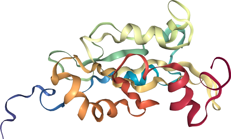
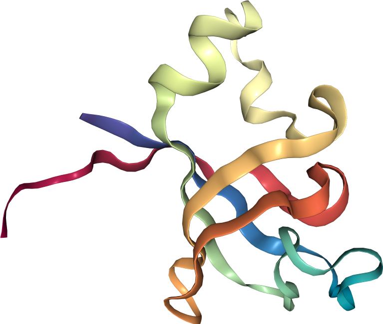
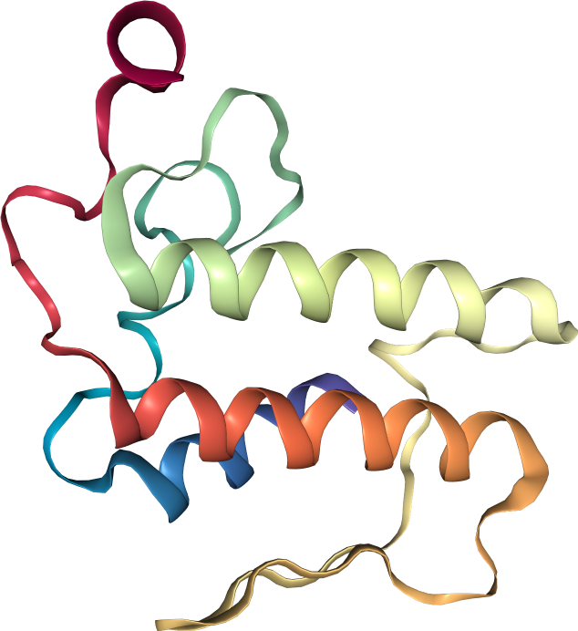
1AK6	1PHT	1POA

Figure 2: Representation of molecules 1AK6, 1PHT, and 1POA for which Coordinate Descent found a global minimizer; while SPG and Gencan found a local minimizer.

	1AK6	1PHT	1POA
Coordinate descent
SPG
Gencan

Figure 3: Molecules 1AK6, 1PHT, and 1POA for which Coordinate Descent found a global minimizer; while SPG and Gencan found a local minimizer. To the naked eye, solutions would appear to be indistinguishable. Therefore, the figures show, for each point $x_{1}^{*},\dots,x_{n_{p}}^{*}$, the value of $E(x_{j}^{*})$ as defined in (59).

At this point the following question arises: how does solving the subproblems with cubically-regularized second-order models affect the performance of the CD method? To answer this question, we solved the same 18 problems tackling the subproblems with quadratically-regularized linear models. This means that, to approximately solve (55) with Algorithm 3.1, we considered $p=1$. In other words, instead of (57,58), (a) we considered the first-order Taylor expansion of $\underline{f}$ at $\bar{x}=x_{\ell(k)}^{k}\in\mathbb{R}^{d}$ given by $M_{\bar{x}}(z):=\underline{f}(\bar{x})+\nabla\underline{f}(\bar{x})^{T}(z-\bar{x})$, and (b) we computed $x^{\mathrm{trial}}$ as the global minimizer of

$$\operatorname*{Minimize}_{z\in\mathbb{R}^{d}}M_{\bar{x}}(z)+\sigma\|z-\bar{x}\|^{2}.$$ (60)

Since (60) has no solution when $\nabla\underline{f}(\bar{x})\neq 0$ and $\sigma=0$, we skip the case $\sigma=0$ by substituting $\sigma\leftarrow 0$ with $\sigma\leftarrow\sigma_{\min}$ at Step 1 of Algorithm 3.1. Apart from this, the settings for the case $p=1$ were identical to those already described for the case $p=2$. Table 3 shows the results. The numbers in the table show that the method found a global solution in all instances, a feature shared with its counterpart with $p=2$. (Only in one instance an alternative global minimizer was found.) The numbers in the table also show that, on average, the method does 1.0001 function evaluations per iteration when $p=2$, while that same amount is 1.5000 when $p=1$. This means that, on the one hand, in the case $p=1$, half of the times the solution of the regularized model is discarded for not satisfying the descent condition and the regularization parameter must be increased. On the other hand, this situation is extremely rare (once every ten thousand iterations) when $p=2$. Moreover, the method with $p=1$ uses, on average, 26 times more iterations, 39 times more function evaluations and 22 times more time than the case $p=2$. The conclusion is that using quadratic models with cubic regularization whose global solution can be calculated using the method introduced in [9], greatly improves the performance of the proposed method.

	Molecule	Coordinate descent with $p=1$
		#iter	#$\underline{f}$	Time	$f(x^{*})$	$E(x^{*})$
ATOM only	1ptq	1,115,103	1,672,658	1.97	9.99e-11	3.98e-05
	1hoe	1,862,919	2,794,382	3.10	9.99e-11	2.04e-06
	1lfb	7,059,295	10,588,949	9.50	9.99e-11	7.52e-06
	1pht	21,056,147	31,584,233	38.52	9.99e-11	2.73e-04
	1poa	107,284,920	160,927,383	105.32	9.99e-11	5.85e-04
	2igg	3,602,906	5,404,362	30.38	9.99e-11	8.43e-06
	1ax8	2,059,932	3,089,901	4.56	9.99e-11	4.05e-06
	1rml	9,186,681	13,780,025	98.21	9.99e-11	3.23e-06
	1ak6	160,256,027	240,384,044	465.43	9.99e-11	1.62e-05
	1a24	79,008,635	118,512,956	238.59	9.99e-11	1.40e-05
	3msp	236,434,288	354,651,435	458.60	9.99e-11	1.61e-05
	3eza	34,134,889	51,202,336	216.98	9.99e-11	1.07e-05
ATOM+HETATM	1ptq	1,466,069	2199,107	2.30	9.97e-11	4.26e-05
	1hoe	683,645	1025,474	3.53	9.99e-11	1.98e-06
	1pht	16,112,116	24168,177	23.29	9.99e-11	3.38e-05
	1poa	32,496,533	48744,802	34.40	9.99e-11	1.46e-02
	1ax8	6,829,569	10244,357	9.37	9.99e-11	2.47e-06
	1rml	2,302,956	3454,437	87.64	9.99e-11	1.99e-06

Table 3: Performance of Coordinate Descent with $p=1$, i.e. considering quadratically-regularized linear models for solving subproblems, applied to the same instances already shown in Table 2.

Another natural question that arises is whether the tendency of the coordinate descent method in finding global minimizers could be observed in a larger set of instances. To check this hypothesis, we downloaded 64 additional random molecules with no more than $6{,}000$ atoms from the ones that were uploaded in 2020; 56 of which have, other than protein atoms, atoms in small molecules. However there were 19 molecules for which, considering protein atoms only or protein atoms plus atoms in small molecules, the graph associated with the incomplete Euclidean matrix obtained by eliminating distances larger than 6 Angstroms is disconnected. Therefore, we were left with 45 and 37 molecules in each set, totalizing 82 new instances. Table 4 shows the performance of Coordinate Descent and SPG when applied to the 45 instances that consider protein atoms only; while Table 5 shows the performance of both methods when applied to the 37 instances that consider protein atoms plus atoms in small molecules. In the 45 instances in Table 4, Coordinate Descent found 37 global minimizers; while SPG found 30 global minimizers. In the 37 instances in Table 5, Coordinate Descent found 30 global minimizers; while SPG found 26 global minimizers.

Molecule	$n$	$n_{p}$	$|S|$	Time $x^{0}$	Coordinate descent					Spectral Projected Gradient
					#iter	#$\underline{f}$	Time	$f(x^{*})$	$E(x^{*})$	#iter	#$f$	Time	$f(x^{*})$	$\|\nabla f(x^{*})\|_{\infty}$	$E(x^{*})$
6kbq	7,554	2,518	98,650 1.56	40.49	10,543,341	10,543,995	36.22	9.99e-11	2.65e-05	810	911	0.96	2.65e-02	7.65e-09	1.87e-01
6kc2	7,530	2,510	98,480 1.56	39.97	7,682,589	7,683,021	20.93	9.99e-11	2.62e-05	954	984	1.11	4.48e-12	3.43e-08	1.29e-05
6khu	3,147	1,049	39,372 3.58	3.09	,316,876	316,959	0.83	9.99e-11	6.12e-06	411	413	0.19	5.66e-11	1.05e-06	7.83e-06
6kir	3,861	1,287	48,596 2.94	5.58	7,574,444	7,574,767	54.37	1.60e-03	1.50e-01	871	895	0.49	5.27e-11	1.01e-07	3.82e-05
6kk9	17,538	5,846	218,662 0.64	479.82	215,549,505	215,561,546	712.59	9.29e-01	1.19e+00	6,262	7,030	17.33	9.09e-01	9.83e-09	1.15e+00
6kki	8,193	2,731	109,472 1.47	53.06	2,113,286	2,113,472	5.68	9.99e-11	5.04e-06	432	434	0.56	9.34e-11	1.33e-07	2.99e-05
6kkj	7,866	2,622	105,642 1.54	47.70	4,068,836	4,070,082	10.88	9.99e-11	5.18e-06	5,868	6,787	7.70	3.24e-10	9.99e-09	1.58e-03
6kkl	8,262	2,754	112,646 1.49	54.76	6,064263	6,064,648	16.61	9.99e-11	5.68e-06	592	604	0.78	9.47e-11	5.99e-08	6.48e-06
6kkv	14,607	4,869	357,016 1.51	290.74	31,543,917	31,545,196	128.60	9.99e-11	1.86e-05	1,095	1,140	4.65	2.88e-11	6.93e-08	2.00e-06
6kx0	9,885	3,295	128,930 1.19	91.69	38,237,232	38,239,417	196.30	1.57e-01	1.02e+00	1,428	1,546	2.26	1.57e-01	9.87e-09	1.02e+00
6kys	5,442	1,814	70,296 2.14	16.13	984,382	984,559	2.49	9.99e-11	4.00e-06	359	360	0.29	8.44e-11	1.22e-07	2.95e-05
6l29	5,427	1,809	70,480 2.15	16.68	965,426	965,620	2.49	9.99e-11	4.51e-06	433	436	0.36	8.43e-11	7.93e-07	8.26e-06
6l2a	2,463	821	29,876 4.44	1.55	411,298	411,381	1.04	9.99e-11	5.55e-06	1,612	1,699	0.59	9.95e-11	7.47e-08	6.46e-05
6laf	8,442	2,814	105,164 1.33	58.06	31,413,895	31,418,665	104.66	9.99e-11	2.51e-05	7,706	9,068	10.22	1.53e-02	9.76e-09	2.74e-01
6li7	7,515	2,505	98,374 1.57	40.21	10,533,446	10,534,072	37.27	9.99e-11	2.64e-05	698	713	0.83	8.73e-11	4.32e-07	1.54e-05
6lik	7,515	2,505	97,354 1.55	39.67	7,579,646	7,580,087	19.88	9.99e-11	2.63e-05	727	749	0.85	8.89e-11	2.61e-07	6.42e-05
6lty	5,964	1,988	73,296 1.86	19.95	3,800,264	3,800,792	9.82	9.99e-11	7.86e-06	672	683	0.58	9.76e-11	9.54e-08	1.78e-05
6ltz	3,432	1,144	41,230 3.15	3.97	,975,177	975,323	2.48	9.99e-11	3.13e-06	8,025	9,404	4.08	1.27e-10	9.94e-09	9.66e-04
6m37	9,999	3,333	125,394 1.13	91.51	130,035,728	130,040,179	422.49	5.07e-02	4.33e-01	4,936	5,479	7.63	5.06e-02	9.99e-09	4.30e-01
6m5n	5,781	1,927	73,890 1.99	18.48	8,183,149	8,183,657	27.54	9.99e-11	6.22e-06	6,419	7,461	5.81	3.06e-03	9.98e-09	2.74e-01
6m6j	759	253	13,914 21.82	0.07	13,076	13,076	0.04	9.99e-11	1.84e-06	59	61	0.01	3.99e-12	1.99e-07	6.82e-07
6m6k	747	249	13,672 22.14	0.07	11,376	11,376	0.04	9.97e-11	1.29e-06	53	55	0.01	2.83e-11	5.59e-07	1.41e-06
6pq0	6,087	2 029	84,104 2.04	22.54	2,346,681	2,346,842	31.31	9.99e-11	3.83e-06	440	442	0.43	2.39e-04	8.43e-09	1.83e-01
6pup	4,035	1,345	50,372 2.79	6.57	544,519	544,617	1.42	9.99e-11	4.87e-06	409	410	0.24	2.52e-11	7.99e-08	2.38e-05
6pxf	4,944	1,648	64,944 2.39	11.70	811,879	812,002	2.13	9.99e-11	2.77e-05	4,907	5,583	3.88	1.81e-10	9.41e-09	2.91e-03
6q08	741	247	13,232 21.78	0.07	22,723	22,744	0.07	9.99e-11	7.19e-06	173	176	0.03	5.75e-11	1.85e-06	3.82e-06
6sx6	2,340	780	44,862 7.38	1.28	143,230	143,260	0.49	9.99e-11	2.50e-06	136	137	0.07	5.51e-12	1.80e-07	2.60e-07
6syk	2,718	906	54,052 6.59	1.99	156,648	156,707	0.55	9.99e-11	2.50e-06	585	592	0.36	9.41e-12	2.34e-07	1.42e-05
6t1z	8,943	2,981	119,580 1.35	65.75	14,818,888	14,819,492	40.30	9.99e-11	8.88e-06	3,247	3,539	4.71	9.94e-11	1.37e-08	2.70e-04
6tad	4,362	1,454	58,736 2.78	8.07	2,385,243	2,385,423	6.35	9.99e-11	6.84e-06	632	643	0.44	7.87e-11	3.81e-07	5.70e-06
6twe	7,902	2,634	163,598 2.36	0.18	5,773,930	5,774,426	20.85	9.99e-11	8.20e-06	598	612	1.16	7.04e-11	1.66e-07	6.93e-06
6ubh	9,009	3,003	113,766 1.26	69.74	8,782,138	8,782,736	22.99	9.99e-11	1.64e-05	3,565	4,019	4.95	1.23e-10	9.86e-09	1.63e-03
6ucd	8,199	2,733	97,910 1.31	52.10	86,618,396	86,621,926	278.99	1.35e+00	1.88e+00	9,391	11,180	11.51	9.92e-01	9.29e-09	1.10e+00
6veh	7,431	2,477	182,676 2.98	42.54	4,087,012	4,087,391	16.46	9.99e-11	1.43e-05	658	662	1.37	3.50e-11	1.38e-07	5.83e-06
6vk2	4,704	1,568	108,520 4.42	11.94	463,141	463,360	1.79	9.99e-11	9.46e-06	3,069	3,419	3.95	1.40e-10	9.62e-09	2.22e-03
6vnz	1,392	464	25,364 11.81	0.32	88,484	88,530	0.29	9.99e-11	3.40e-06	206	208	0.06	6.02e-11	2.16e-07	4.36e-06
6vv6	7,464	2,488	92,878 1.50	45.42	7,583,602	7,584,292	33.37	9.99e-11	4.04e-06	1,846	1,943	2.05	6.23e-02	1.00e-08	2.23e-01
6vv7	7,452	2,484	93,102 1.51	44.46	7,692,189	7,692,886	41.06	9.99e-11	3.80e-06	1,981	2,233	2.26	1.07e-01	7.39e-09	2.23e-01
6vv9	7,452	2,484	92,506 1.50	44.29	6,251,096	6,251,759	29.79	9.99e-11	3.11e-06	1,022	1,040	1.14	7.95e-02	1.25e-09	2.17e-01
6wcr	11,766	3,922	151,164 0.98	158.07	118,185,068	118,209,777	421.33	1.67e-01	3.74e-01	7,460	8,498	13.92	1.99e-01	9.96e-09	2.38e-01
6yuc	8,637	2,879	107,258 1.29	60.03	17,737,727	17,738,988	117.20	3.77e-01	6.86e-01	1,450	1,668	1.91	1.09e-04	9.93e-09	1.19e-01
6z4c	5,838	1,946	72,838 1.92	18.87	1,951,179	1,951,337	5.00	9.99e-11	2.72e-06	369	370	0.31	6.24e-11	2.43e-07	2.91e-06
6zcm	7,899	2,633	102,030 1.47	46.05	12,338,443	12,339,335	40.78	9.99e-11	2.53e-05	7,445	8,812	9.41	1.38e-10	9.93e-09	9.87e-04
7ckj	4,731	1,577	59,608 2.40	10.24	2,681,962	2,682,163	11.61	9.99e-11	3.27e-06	768	784	0.54	6.51e-07	5.85e-09	2.03e-01
7jjl	9,690	3,230	125,976 1.21	83.34	77,851,519	77,854,837	303.65	4.82e-01	4.52e-01	4,830	5,451	7.49	7.94e-01	8.12e-09	4.73e-01

Table 4: Performance of Coordinate Descent and SPG methods in the 46 instances that consider protein atoms only.

Molecule	$n$	$n_{p}$	$|S|$	Time $x^{0}$	Coordinate descent					Spectral Projected Gradient
					#iter	#$\underline{f}$	Time	$f(x^{*})$	$E(x^{*})$	#iter	#$f$	Time	$f(x^{*})$	$\|\nabla f(x^{*})\|_{\infty}$	$E(x^{*})$
6kbq	8,106	2,702	108,066 ( 1.48%)	50.64	6,476,123	6,476,435	17.57	9.99D-11	2.35D-05	571	580	0.71	9.97D-11	6.32D-08	1.85D-05
6kc2	8,397	2,799	111,198 ( 1.42%)	56.89	15,115,487	15,118,534	50.50	9.99D-11	2.15D-01	1,102	1,121	1.42	4.03D-10	9.36D-09	2.19D-01
6khu	3,465	1,155	44,672 ( 3.35%)	4.24	334,415	334,473	0.87	9.99D-11	6.35D-06	490	500	0.25	6.20D-11	1.63D-06	7.45D-06
6kir	4,203	1,401	54,634 ( 2.79%)	7.42	560,278	560,406	1.49	9.99D-11	4.20D-06	450	454	0.28	9.28D-11	4.63D-07	6.28D-05
6kk9	17,895	5,965	225,776 ( 0.63%)	515.33	202,467,161	202,477,953	691.77	4.00D-01	3.09D-01	5,084	5,637	13.87	3.82D-01	9.95D-09	3.70D-01
6kki	8,364	2,788	111,596 ( 1.44%)	56.23	2,049,210	2,049,408	5.51	9.99D-11	3.93D-06	592	594	0.76	9.92D-11	1.13D-07	5.68D-05
6kkj	7,992	2,664	106,472 ( 1.50%)	49.62	17,809,921	17,816,613	132.85	9.54D-04	2.81D-01	2,921	3,188	3.67	9.54D-04	9.12D-09	2.81D-01
6kkl	8,421	2,807	114,184 ( 1.45%)	58.35	6,082,607	6,082,924	16.57	9.99D-11	5.67D-06	521	537	0.70	6.88D-11	2.32D-07	6.82D-06
6kkv	14,820	4,940	364,756 ( 1.49%)	304.81	27,357,834	27,358,998	113.43	9.99D-11	1.80D-05	1,193	1,220	5.01	7.35D-10	7.99D-09	4.74D-05
6kx0	10,044	3,348	131,624 ( 1.17%)	94.64	45,983,700	45,985,561	226.68	7.16D-02	2.47D-01	1,044	1,096	1.61	1.78D-01	9.27D-09	1.01D+00
6kys	5,886	1,962	77,926 ( 2.03%)	20.28	816,852	816,930	2.19	9.99D-11	3.60D-06	2,389	2,688	2.22	9.98D-11	3.11D-08	1.72D-04
6l29	5,841	1,947	77,602 ( 2.05%)	19.25	1,807,474	1,807,572	18.75	9.99D-11	1.26D-01	589	592	0.52	5.31D-04	4.39D-09	1.60D-01
6l2a	2,643	881	32,644 ( 4.21%)	1.82	787,753	787,881	4.57	9.99D-11	5.77D-06	1,769	1,892	0.67	1.79D-10	9.03D-09	1.24D-01
6laf	8,535	2,845	106,084 ( 1.31%)	57.40	38,880,745	38,890,853	174.71	1.57D-02	3.40D-01	10,824	12,773	13.95	1.71D-02	9.71D-09	3.41D-01
6li7	8,520	2,840	114,120 ( 1.42%)	57.40	6,141,620	6,141,906	16.33	9.99D-11	2.29D-05	443	453	0.58	9.37D-11	5.62D-08	1.50D-05
6lik	8,208	2,736	108,364 ( 1.45%)	51.66	12,686,358	12,686,897	52.81	9.99D-11	2.48D-05	7,235	8,363	9.40	2.99D-03	9.91D-09	1.81D-01
6ltz	3,798	1,266	47,246 ( 2.95%)	5.62	767,531	767,612	1.93	9.99D-11	7.56D-06	985	1,002	0.54	9.73D-11	5.68D-08	1.28D-04
6m5n	6,687	2,229	88,996 ( 1.79%)	29.41	2,380,904	2,381,175	6.33	9.99D-11	1.41D-01	14,921	17,730	15.90	6.98D-10	9.55D-09	1.42D-01
6m6j	840	280	15,602 (19.97%)	0.09	18,319	18,319	0.06	9.99D-11	1.86D-06	76	78	0.01	9.94D-11	3.25D-07	2.06D-06
6m6k	828	276	15,388 (20.27%)	0.09	15,964	15,964	0.05	9.99D-11	1.63D-06	74	76	0.01	1.00D-11	3.36D-07	7.45D-07
6pq0	6,360	2,120	89,018 ( 1.98%)	0.12	1,086,898	1,086,994	12.19	9.99D-11	3.98D-06	3,540	4,285	3.81	9.00D-11	1.21D-07	6.60D-05
6pup	4,272	1,424	55,442 ( 2.74%)	7.63	593,071	593,135	1.55	9.99D-11	3.60D-06	363	372	0.23	3.28D-11	6.55D-07	2.12D-06
6pxf	5,661	1,887	76,154 ( 2.14%)	17.47	6,753,157	6,775,873	25.50	9.97D-11	1.10D-01	4,541	5,069	4.07	1.04D-05	9.49D-09	1.16D-01
6t1z	9,492	3,164	127,488 ( 1.27%)	79.93	3,427,330	3,427,847	9.17	9.99D-11	1.14D-02	7,688	9,017	11.70	2.94D-10	9.82D-09	1.23D-02
6tad	5,172	1,724	71,178 ( 2.40%)	13.52	1,050,635	1,050,702	2.89	9.99D-11	3.64D-06	273	275	0.22	9.83D-11	3.61D-08	3.95D-06
6twe	7,905	2,635	163,694 ( 2.36%)	45.84	5,768,235	5,768,740	20.83	9.99D-11	8.19D-06	637	643	1.17	9.14D-11	1.78D-07	8.01D-06
6ubh	9,999	3,333	130,348 ( 1.17%)	91.62	22,598,823	22,602,027	107.35	9.99D-11	3.60D-01	1,234	1,279	1.90	6.89D-11	3.25D-07	3.63D-01
6veh	7,566	2,522	186,586 ( 2.93%)	42.40	4,241,879	4,242,258	17.14	9.99D-11	1.52D-05	381	384	0.80	8.74D-11	2.80D-07	4.54D-05
6vv6	8,169	2,723	107,072 ( 1.44%)	52.54	2,824,276	2,824,520	7.62	9.99D-11	9.75D-06	391	395	0.49	7.43D-11	8.50D-08	3.05D-06
6vv7	8,247	2,749	109,326 ( 1.45%)	52.54	3,807,178	3,807,395	10.23	9.99D-11	2.33D-06	4,434	5,002	5.83	5.68D-11	3.59D-07	2.89D-04
6vv9	8,250	2,750	108,784 ( 1.44%)	52.41	3,494,562	3,494,812	9.30	9.99D-11	8.41D-06	404	409	0.51	6.69D-11	2.00D-07	7.49D-06
6wcr	12,225	4,075	157,032 ( 0.95%)	167.40	229,852,446	229,885,273	721.26	9.77D-05	8.68D-02	6,972	7,906	13.17	8.93D-02	9.97D-09	1.97D-01
6yuc	8,640	2,880	107,366 ( 1.29%)	59.34	50,987,720	50,988,983	203.00	1.09D-04	1.19D-01	1,879	1,942	2.37	1.09D-04	7.65D-09	1.19D-01
6z4c	5,994	1,998	76,300 ( 1.91%)	20.35	1,697,728	1,697,882	4.45	9.99D-11	2.95D-06	270	271	0.24	9.71D-11	2.20D-07	3.12D-06
6zcm	9,696	3,232	135,448 ( 1.30%)	83.59	6,978,627	6,978,943	19.30	9.99D-11	7.42D-06	2,131	2,288	3.43	9.67D-11	5.81D-08	1.55D-04
7ckj	5,199	1,733	68,624 ( 2.29%)	13.55	1,630,610	1,630,694	10.52	9.99D-11	4.11D-06	541	549	0.43	2.14D-05	9.60D-09	1.96D-01
7jjl	9,693	3,231	126,082 ( 1.21%)	83.84	102,233,476	102,237,339	369.96	2.46D-01	3.25D-01	5,332	6,097	8.12	7.94D-01	8.91D-09	4.73D-01

Table 5: Performance of Coordinate Descent and SPG methods in the 37 instances that consider protein atoms plus atoms in small molecules.

8 Conclusions

Methods based on high-order models for optimization are difficult to implement due to the necessity of computing and storing high-order derivatives and the complexity of solving the subproblems. These difficulties are not so serious if the subproblems are low-dimensional, which is the most frequent situation in the case of CD methods. In the extreme case, in which one solves only univariate problems, the number of high-order partial derivatives that are necessary is a small multiple of the number of variables. Therefore, the theory that shows that CD algorithms with high-order models enjoy good convergence and complexity properties seems to be useful to support the efficiency of practical implementations. In this context, higher-order techniques allow to escape from attraction points that tend to satisfy lower-order optimality conditions; see [49].

Sometimes the fulfillment of a necessary high-order optimality condition can be expressed as fulfillment of $\Phi(x)=0$, where $\Phi$ is a continuous nonnegative function. In this case, it makes sense to say that $\Phi(x)\leq\varepsilon$ is an approximate high-order optimality condition. Moreover, instead of requiring globality for the solution to the regularized model-based subproblem (18), we may require only that $\Phi(x^{k+1})\to 0$ when $k\to+\infty$, where $\Phi$ corresponds to the high-order optimality condition of (18). Careful choices of $\Phi$ and the subproblems’ stopping criterion may give rise to complexity results associated with the attainment of these high-order optimality conditions, see [27, 28, 29]. This will be the subject of future research.

In this paper the defined algorithms were applied to the identification of proteins under NMR data. Moreover, we extended the CD approach to the computation of a suitable initial approximation that avoids, in many cases, the convergence to local non-global minimizers. Our choice of the most adequate parameter $p$, that defines the approximating models, and the strategy for choosing the groups of variables were dictated by theoretical considerations discussed in Section 6 and by the specific characteristics of the problem. Our computing results are fully reproducible and the codes are available in http://www.ime.usp.br/~egbirgin/.

In future works we will apply the new CD techniques to the case in which data uncertainty is present and outliers are likely to occur. Possible improvements also include the choice of different models at each iteration or at each group of variables with the aim of making a better use of current information.

Data availability: The datasets generated during and/or analyzed during the current study are available in the corresponding author web page, http://www.ime.usp.br/~egbirgin/.

References

- [1] F. J. Aragón Artacho, J. M. Borwein, and M. K. Tam, Douglas-Rachford feasibility methods for matrix completion problems, The ANZIAM Journal 55, pp. 299–326, 2014.
- [2] H. Attouch, J. Bolte, P. Redont, and A. Soubeyran, Proximal alternating minimization and projection methods for nonconvex problems: an approach based on the Kurdyka-Lojasiewicz inequality, Mathematics of Operations Research 38, pp. 438–457, 2010.
- [3] A. Beck and L. Tetruashvili, On the convergence of block coordinate descent methods, SIAM Journal on Optimization 23, pp. 2037–2060, 2013.
- [4] S. Bellavia, G. Gurioli, B. Morini, and Ph. L. Toint, Adaptive regularization algorithms with inexact evaluations for nonconvex optimization, SIAM Journal on Optimization 29, pp. 2881-2915, 2019.
- [5] E. G. Birgin, J. L. Gardenghi, J. M. Martínez, and S. A. Santos, On the use of third-order models with fourth-order regularization for unconstrained optimization, Optimization Letters 14, pp. 815–838, 2020.
- [6] E. G. Birgin, J. L. Gardenghi, J. M. Martínez, S. A. Santos, and Ph. L. Toint, Worst-case evaluation complexity for unconstrained nonlinear optimization using high-order regularized models, Mathematical Programming 163, pp. 359–368, 2017.
- [7] E. G. Birgin and J. M. Martínez, Large-scale active-set box-constrained optimization method with spectral projected gradients, Computational Optimization and Applications 23, pp. 101–125, 2002.
- [8] E. G. Birgin and J. M. Martínez, On regularization and active-set methods with complexity for constrained optimization, SIAM Journal on Optimization 28, pp.1367–1395, 2018.
- [9] E. G. Birgin and J. M. Martínez, A Newton-like method with mixed factorizations and cubic regularization for unconstrained minimization, Computational Optimization and Applications 73, pp. 707–753, 2019.
- [10] E. G. Birgin and J. M. Martínez, Complexity and performance of an Augmented Lagrangian algorithm, Optimization Methods and Software 35, pp. 885–920, 2020.
- [11] E. G. Birgin, J. M. Martínez, and M. Raydan, Nonmonotone spectral projected gradient methods on convex sets, SIAM Journal on Optimization 10, pp. 1196–1211, 2000.
- [12] E. G. Birgin, J. M. Martínez, and M. Raydan, Algorithm 813: SPG - software for convex-constrained optimization, ACM Transactions on Mathematical Software 27, pp. 340–349, 2001.
- [13] E. G. Birgin, J. M. Martínez, and M. Raydan, Spectral Projected Gradient methods: Review and Perspectives, Journal of Statistical Software 60(3), pp. 1–21, 2014.
- [14] E. G. Birgin, J. M. Martínez, and M. Raydan, Spectral Projected Gradient methods, in C. Floudas and P. Pardalos (eds.) Encyclopedia of Optimization, Springer, Boston, MA, 2008, pp. 3652–3659.
- [15] J. Bolte, S. Sabach and M. Teboulle, Proximal alternating linearized minimization of nonconvex and nonsmooth problems, Mathematical Programming 146. pp. 1–36, 2014.
- [16] S. Bonettini, M. Prato, and S. Begegoldi, A cyclic block coordinate descent method with generalized gradient projections, Applied Mathematics and Computation 286, pp. 288–300, 2016.
- [17] C. A. Bouman and K. Sauer, A unified approach to statistical tomography using coordinate descent optimization, IEEE Transactions on Image Processing 5, pp. 480–492, 1996.
- [18] S. Boyd, N. Parikh, E. Chu, B. Peleato, and J. Eckstein, Distributed optimization and statistical learning via the alternating direction method of multipliers, Foundations and Trends in Machine Learning 3, pp. 1–122, 2011.
- [19] C. P. Bras, J. M. Martínez, and M. Raydan, Large-scale unconstrained optimization using separable cubic modeling and matrix-free subspace minimization, Computational Optimization and Applications 75, pp. 169–205, 2020.
- [20] P. Breheny and J. Huang, Coordinate descent algorithms for nonconvex penalized regression with applications to biological feature selection, Annals of Applied Statistics 5, pp. 232–252, 2011.
- [21] H. Calandra, S. Gratton, E. Riccietti, and X. Vasseur, On high-order multilevel optimization strategies, SIAM Journal on Optimization 31, pp. 307–330, 2021.
- [22] C. Cartis, N. I. M. Gould, and Ph. L. Toint, Adaptive cubic regularization methods for unconstrained optimization. Part I: motivation motivation, convergence and numerical results, Mathematical Programming 127, pp. 245–295, 2011.
- [23] C. Cartis, N. I. M. Gould, and Ph. L. Toint, Adaptive cubic regularization methods for unconstrained optimization. Part II: worst-case function and derivative complexity, Mathematical Programming 130, pp. 295–319, 2011.
- [24] C. Cartis, N. I. M. Gould, and Ph. L. Toint, Universal regularization methods - varying the power, the smoothness and the accuracy, SIAM Journal on Optimization 29, pp. 595–615, 2019.
- [25] C. Cartis, N. I. M. Gould, and Ph. L. Toint, Improved worst-case evaluation complexity for potentially rank-deficient nonlinear least-Euclidean-norm problems using higher-order regularized models, Technical Report naXys-12-2015, Namur Center for Complex Systems, University of Namur, Belgium, 2015.
- [26] C. Cartis, N. I. M. Gould, and Ph. L. Toint, Worst-case evaluation complexity for regularization models for smooth unconstrained optimization using Hölder-continuous gradients, Optimization Methods and Software 6, pp. 1273–1298, 2017.
- [27] C. Cartis, N. I. M. Gould, and Ph. L. Toint, Second-order optimality and beyond: characterization and evaluation complexity in convexly-constrained nonlinear optimization, Foundations of Computational Mathematics 18, pp. 1073–1107, 2018.
- [28] C. Cartis, N. I. M. Gould, and Ph. L. Toint, Sharp worst-case evaluation complexity bounds for arbitrary-order nonconvex optimization with inexpensive constraints, SIAM Journal on Optimization 30, pp. 513–541, 2020.
- [29] C. Cartis, N. I. M. Gould, and Ph. L. Toint, Strong evaluation complexity bounds for arbitrary-order optimization of nonconvex nonsmooth composite functions, arXiv preprint arXiv:2001.10802, 2020.
- [30] A. A, Canutescu and R. L. Dunbrack, Cyclic coordinate descent: a robotics algorithm for protein loop closure, Protein Science 12, pp. 963–972, 2003.
- [31] X. Chen and Ph. L. Toint, High-order evaluation complexity for convexly-constrained optimization with non-Lipschitzian group sparsity terms, Mathematical Programming 187, pp. 47–78, 2021.
- [32] T. F. Cox and M. A. A. Cox, Multidimensional Scaling, 2nd. ed., Chapman and Hall/CRC, New York, NY, USA, 2001.
- [33] F. E. Curtis, D. P. Robinson, and M. Samadi, A trust-region algorithm with a worst-case iteration complexity of , Mathematical Programming 162, pp. 1–32, 2017.
- [34] F. E. Curtis, D. P. Robinson, and M. Samadi, An inexact regularized Newton framework with a worst-case iteration complexity of for nonconvex optimization, IMA Journal of Numerical Analysis, pp. 1–32, 2018.
- [35] J. P. Dussault, ARCq: a new adaptive regularization by cubics, Optimization Methods and Software 33, pp. 322–335, 2018.
- [36] J. Eckstein and W. Yao, Understanding the convergence of the alternating direction method of multipliers: Theoretical and computational perspectives, Pacific Journal of Optimization 11, pp. 619–644, 2015.
- [37] H.-R. Fang and D. P. O’Leary, Euclidean distance matrix completion problems, Optimization Methods and Software 27, pp. 695–717, 2012.
- [38] W. Glunt, T. L. Hayden, and M. Raydan, Molecular conformations from distance matrices, Journal of Computational Chemistry 14, pp. 114–120, 1993.
- [39] G. N. Grapiglia and Y. Nesterov, Regularized Newton methods for minimizing functions with Hölder continuous Hessians, SIAM Journal on Optimization 27, pp. 478–506, 2017.
- [40] G. N. Grapiglia and Y. Nesterov, Tensor methods for minimizing functions with Hölder continuous higher-order derivatives, SIAM Journal on Optimization 30, pp. 2750–2779, 2020.
- [41] G. N. Grapiglia, J-Y Yuan, and Y-X Yuan, On the convergence and worst-case complexity of trust-region and regularization methods for unconstrained optimization, Mathematical Programming 152, pp. 491–520, 2015.
- [42] S. Gratton, E. Simon, and Ph. L. Toint, An algorithm for the minimization of nonsmooth nonconvex functions using inexact evaluations and its worst-case complexity, Mathematical Programming 187, pp. 1–24, 2021.
- [43] A. Griewank, The modification of Newton’s method for unconstrained optimization by bounding cubic terms, Technical Report NA/12, Department of Applied Mathematics and Theoretical Physics, University of Cambridge, 1981.
- [44] C. Lavor, L. Liberti, and N. Maculan, Molecular Distance Geometry Problem, in C. Floudas and P. Pardalos (eds.) Encyclopedia of Optimization, Springer, Boston, MA, 2008, pp. 2304–2311.
- [45] L. Liberti, C. Lavor, N. Maculan, and A. Mucherino, Euclidean distance geometry and applications, SIAM Review 56, pp. 3–69, 2014.
- [46] T. Lin and M. I. Jordan, A control-theoretic perspective on optimal high-order optimization, Mathematical Programming, to appear (DOI: 10.1007/s10107-021-01721-3).
- [47] Q. Lin, Z. Lu, and L. Xiao, An accelerated proximal coordinate descent method and its application to empirical risk minimization, arXiv preprint arXiv:1407.1296, 2014.
- [48] J. M. Martínez, On high-order model regularization for constrained optimization, SIAM Journal on Optimization 27, pp. 2447–2458, 2017.
- [49] J. M. Martínez and M. Raydan, Separable cubic modeling and a trust-region strategy for unconstrained minimization with impact in global optimization, Journal of Global Optimization 63, pp. 315–342, 2015.
- [50] J. M. Martínez and M. Raydan, Cubic-regularization counterpart of a variable-norm trust-region method for unconstrained minimization, Journal of Global Optimization 68, pp. 367–385, 2017.
- [51] A. Mead, Review of the development of multidimensional scaling methods, Journal of the Royal Statistical Society. Series D (The Statistician) 41, pp. 27-–39, 1992.
- [52] Y. Nesterov, Efficiency of coordinate descent methods on huge-scale optimization problems, SIAM Journal on Optimization 22, pp. 341–362, 2012.
- [53] Y. Nesterov and B. T. Polyak, Cubic regularization of Newton’s method and its global performance, Mathematical Programming 108, pp. 177–205, 2006.
- [54] M. S. Petković, B. Neta, L. S. Petković, and J. Džunic, Multipoint methods for solving nonlinear equations: A survey, Applied Mathematics and Computation 226, pp. 635–660, 2014.
- [55] M. J. D. Powell , On search directions for minimization algorithms, Mathematical Programming 4, pp. 193–201, 1973.
- [56] C. W. Royer and S. J. Wright, Complexity analysis of second-order line-search algorithms for smooth nonconvex optimization, SIAM Journal on Optimization 28, pp. 1448–1477, 2018.
- [57] W. S. Torgerson, Theory & Methods of Scaling, John Wiley and Sons, New York, NY, USA, 1958.
- [58] S. J. Wright, Coordinate descent methods, Mathematical Programming 151, pp. 3–34, 2015.
- [59] https://www.rcsb.org, accessed on August, 14th, 2020.
- [60] Y. Xu and W. Yin, A globally convergence algorithm for nonconvex optimization based on block coordinate update, Journal of Scientific Computing 72, pp. 700–734, 2017.
- [61] J. C. Yu, K. J. Webb, C. A. Bouman, and R. P. Milane, Optical diffusion tomography by iterative coordinate-descent optimization in a Bayesian framework, Journal of the Optical Society of America A 16, pp. 2400–2412, 1999.
- [62] X. Zhu, J. Han, and B. Jiang, An adaptive high-order method for finding third-order critical points of nonconvex optimization, arXiv preprint arXiv:2008.04191, 2020.