A SModelS interface for pyhf likelihoods

Abstract

SModelS is an automatized tool enabling the fast interpretation of simplified model results from the LHC within any model of new physics respecting a $\mathbb{Z}_{2}$ symmetry. We here present a new version of SModelS, which can use the full likelihoods now provided by ATLAS in the form of pyhf JSON files. This much improves the statistical evaluation and therefore also the limit setting on new physics scenarios.

1 Introduction

An essential step for interpretation of experimental results is the construction of a statistical model, or likelihood, to compare the observed data to the target theory. Given the likelihood, all the standard statistical approaches are available for extracting information from it.

Therefore, Ref. [1] recommended for the presentation of LHC results: ”When feasible, provide a mathematical description of the final likelihood function in which experimental data and parameters are clearly distinguished, either in the publication or the auxiliary information. Limits of validity should always be clearly specified.” And furthermore “Additionally provide a digitized implementation of the likelihood that is consistent with the mathematical description.” These are the Les Houches Recommendations 3(b) and 3(c). The necessity of detailed likelihood information was further elaborated in the recent report of the LHC Reinterpretation Forum [2].

Among the major benefits of detailed likelihood information for reinterpretation is the fact that it allows one to statistically combine disjoint signal regions (SRs) instead of using only the most sensitive (a.k.a. “best”) SR; see, e.g., [3, 4] for the impact in physics studies.

The CMS SUSY group has been publishing SR correlation data in the form of covariance matrices for some of their analyses. This so-called simplified likelihood [5] approach assumes that uncertainties can be well approximated by Gaussians. SModelS [6, 7, 8] can make use of these correlation data since its version 1.2 [8]; their benefit for limit setting was demonstrated in [8] and contribution 15 of [9].

ATLAS has recently gone a significant step further by publishing full likelihoods using a JSON serialization [11], which provides background estimates, changes under systematic variations, and observed data counts at the same fidelity as used in the experiment. The JSON format describes the HistFactory family of statistical models [12], which is used by the majority of ATLAS searches. The pyhf package [13] is then used to construct statistical models, and perform statistical inference, within a python environment. Note that this fulfills for the first time the Les Houches Recommendations 3(b,c)!

In the following we describe the usage of the ATLAS pyhf  likelihoods in SModelS. We also demonstrate the improvements in the statistical evaluation —and thus in the constraining power—due to these likelihoods. Readers who are not already familiar with SModelS are referred to [6, 7, 8, 14, 15] for details on the tool and how to use it. Further information, including a detailed online manual, is available at https://smodels.github.io/.

2 Usage in SModelS

The pyhf JSON files [11] from ATLAS report $L(\theta|\mathcal{D})$, where $\theta$ is the union of parameters of interest and possible nuisance parameters and $\mathcal{D}$ denotes the observed data. Encoded in this way are, in particular, background estimates, correlations, and primary data. Together with the relevant simplified model efficiency maps, they allow SModelS to evaluate the likelihood of the signal strength of a hypothesized signal in a realistic manner.

To make use of this machinery, besides scipy and numpy, which are already required by SModelS, the following python packages need to be installed:

pyhf, jsonpatch, jsonschema.

In addition, for speed reasons, we recommend pytorch as backend for pyhf (if not available, the default backend will be used). Details are given in the online manual at https://smodels.readthedocs.io/en/stable/Installation.html. Details on the pyhf package are given in [13] and at https://scikit-hep.org/pyhf/.

2.1 Implementation in the database

In the SModelS database, the JSON files are placed in the respective analysis folder that holds the simplified model efficiency maps (see [7] for the database structure). The information, which JSON file is used to combine which SRs, is given in the globalInfo.txt file in each analysis folder. For example, for the ATLAS stau search [16], which has two SRs, the globalInfo.txt file contains:

  id: ATLAS-SUSY-2018-04
  ....
  datasetOrder: "SRlow", "SRhigh"
  jsonFiles: {"SRcombined.json": ["SRlow", "SRhigh"]}

In case the provided JSON files describe the combination of one or more subsets of SRs, as in the multi-$b$ sbottom search [17], the format is:

  id: ATLAS-SUSY-2018-31
  ....
  datasetOrder: "SRA_L", "SRA_M", "SRA_H", "SRB", "SRC_22",
                "SRC_24", "SRC_26", "SRC_28"
  jsonFiles: {"BkgOnlyA.json": ["SRA_L", "SRA_M", "SRA_H"],
              "BkgOnlyB.json": ["SRB"],
              "BkgOnlyC.json": ["SRC_22", "SRC_24", "SRC_26",
                                "SRC_28"]}

Here, the likelihoods for SRs A, B and C will first be evaluated separately, and then only the most sensitive result among SRA, SRB and SRC will be used for the limit setting.

2.2 Changes/additions in the SModelS code

The interfacing of pyhf to SModelS can be summarized in two parts: the addition of an independent module tools/pyhfInterface.py, and the changes brought to experiment/datasetObj.py.

The tools/pyhfInterface.py module is made of two classes, PyhfData, storing and handling informations related to the JSON files and input signal predictions, and PyhfUpperLimitComputer, where the upper limits are inferred given the PyhfData information. The constructor of PyhfData takes as arguments nsignals and inputJsons, which are respectively the list of BSM prediction yields and the list of workspaces, i.e., the likelihoods as python JSON objects [18]. The list of signal yields is a 2-dimensional list, so that there is a sublist for each JSON likelihood. For the previous example

  jsonFiles: {"BkgOnlyA.json": ["SRA_L", "SRA_M", "SRA_H"],
              "BkgOnlyB.json": ["SRB"],
              "BkgOnlyC.json": ["SRC_22", "SRC_24", "SRC_26",
                                "SRC_28"]}

the nsignals would read

  nsignals = [[<SRA_L>, <SRA_M>, <SRA_H>],
              [<SRB>],
              [<SRC_22>, <SRC_24>, <SRC_26>, <SRC_28>]]

where SRA_L> }, {\verb SRA_M¿ , … are the event yield predictions in the signal regions named SRA_L , SRA_M , …, respectively.

The JSON likelihoods provided by ATLAS are written in the following python dictionary structure:

    {"channels":[
        {"name":..., "samples":[
            {"data":[...], "modifiers":[...]},
            {"data":[...], "modifiers":[...]},
            ...
            ]
        },
        {"name":..., "samples":[...],
        ...
        ]
    }

where the channels are the usual signals regions, and the samples contain the different background contributions. In each sample, data contains the event yields and modifiers is the list of all the modifiers representing the uncertainties. The hypothesized BSM signal will be added in the form of one of these samples.

The PyhfData constructor first collects information in the workspaces such as the number of SRs, and the paths to the samples where the BSM predictions are to be written, and also the virtual regions (VRs) and control regions (CRs) that are assumed not to contribute and are then removed from the workspaces. It must be noted that this approximation can imply a slight loss in accuracy because any potential leakage of the signal into the VRs or CRs is neglected. The fetched information in the inputJsons is then compared to the nsignals to check for any inconsistencies in the format of the two variables.

The jsonpatch package [19] allows to easily write into an existing JSON object. The PyhfUpperLimitComputer class uses this feature to add the BSM prediction yields and remove the control and virtual regions from the workspaces. This procedure is dynamical so that the signal predictions can be re-scaled throughout the statistical inference.

The pyhf.infer.hypotest allows to compute the $\textrm{CL}_{s}$ [20] with a signal strength modifier $\mu$ as argument, using the asymptotic formulae from [21]. Upper limits are found by varying the $\textrm{CL}_{s}$ with respect to $\mu$. Namely, our pyhf interface will look for the $\mu$ at $95\%$ exclusion confidence level (CL). $\mu$ being a multiplicative factor, the unit of the obtained upper limit will depend on the unit of the signal predictions provided. In our case, normalised signals give unitless upper limits on the event yields. We first dynamically rescale the signal predictions, so that $\mu$ at $95\%$ CL lies in the interval $[0.2,\,5]$, and then use the optimize feature of the scipy package [22] to find the exclusion limit at $95\%$ CL.

The independent tools/pyhfInterface.py module is interfaced to SModelS in experiment/datasetObj.py, as it is for the simplified likelihood. If combination is requested and JSON files are found in the database, the code in datasetObj.py will perform pyhf combination. If more than one JSON file is provided, ”best expected combination” is performed, i.e., the upper limit is computed using the JSON that gives the most sensitive combination.

2.3 Running SModelS

The interface to pyhf is available from SModelS v1.2.4 onward. Running the program has not changed with respect to previous versions, apart from setting a switch to evoke the (optional) use of the JSON files in the database. When using runSModelS.py, one has to set

   combineSRs = True

in the paramerers.ini file. Note that the same flag also turns on the SR combination in the simplified likelihood approach for CMS efficiency map results, for which a covariance matrix is available.

Alternatively, one can call theoryPredictionsFor() with the option combinedResults=True in one’s own python program, cf. the Example.py file in the SModelS v1.2.4 distribution.

3 Validation and physics impact

We compare in Figure 1 the SModelS exclusion (grey line) with the official exclusion (black line) for the ATLAS stau search [16], using best SR (left) and using pyhf combination (right). As one can see, the usual procedure, which picks up the most sensitive efficiency map result, over-excludes by about 50 GeV on half the exclusion line. In contrast, a very good agreement with the official ATLAS result is obtained with the full pyhf likelihood.

Figure 2 shows the same kind of validation for the ATLAS sbottom search [17], which was actually the first one to provide the full likelihood. In this case, without pyhf, SModelS is under-excluding by roughly 50–100 GeV. Again we observe a significant improvement with the pyhf combination.

Our third example, shown in Figure 3, is for the ATLAS electroweakino search in the $W(\to\ell\nu)h(\to b\bar{b})+E_{T}^{\rm miss}$ channel [23]. Using the best exclusive SR (left panel in Figure 3), we face an under-exclusion over almost the entire mass plane. Using instead the best inclusive SR (not shown) would give a SModelS limit closer to the official one for large mass differences, but lead to a serious over-exclusion for small mass differences. The combination of SRs based on the full likelihood resolves these problems, and we obtain a good agreement of the SModelS exclusion line with the official one from ATLAS as shown in the right panel of Figure 3.

Figure 1: Validation of TStauStau ($pp\to\tilde{\tau}_{1}^{+}\tilde{\tau}_{1}^{-}$, $\tilde{\tau}^{\pm}_{1}\to\tau\tilde{\chi}^{0}_{1}$) result from the ATLAS stau search [16], on the left using the best SR, on the right using the full likelihood.

Figure 2: Validation of the T6bbHH ($pp\to\tilde{b}_{1}\tilde{b}_{1}^{*}$, $\tilde{b}_{1}\to b\tilde{\chi}^{0}_{2}$, $\tilde{\chi}^{0}_{2}\to h\tilde{\chi}^{0}_{1}$) result from the ATLAS sbottom search [17], on the left using the best SR, on the right using the full likelihood.

Figure 3: Validation of the TChiWH ($pp\to\tilde{\chi}_{2}^{0}\tilde{\chi}_{1}^{\pm}$, $\tilde{\chi}_{2}^{0}\to h\tilde{\chi}^{0}_{1}$, $\tilde{\chi}^{\pm}_{1}\to W\tilde{\chi}^{0}_{1}$) result from the ATLAS electroweakino search [23], on the left using the best SR, on the right using the full likelihood.

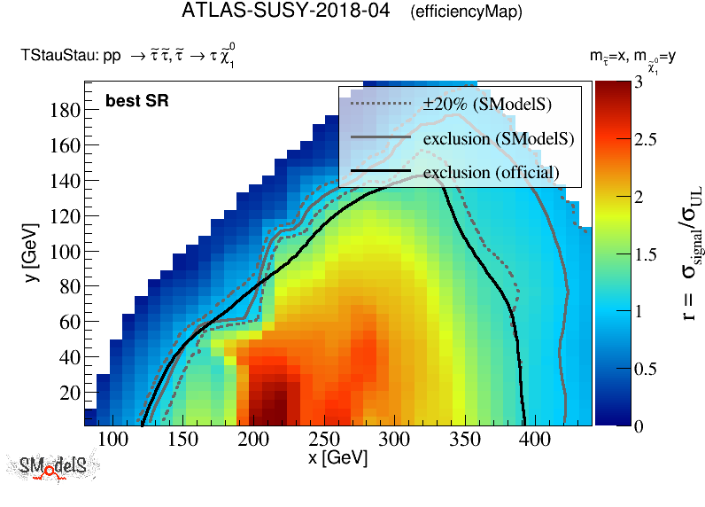
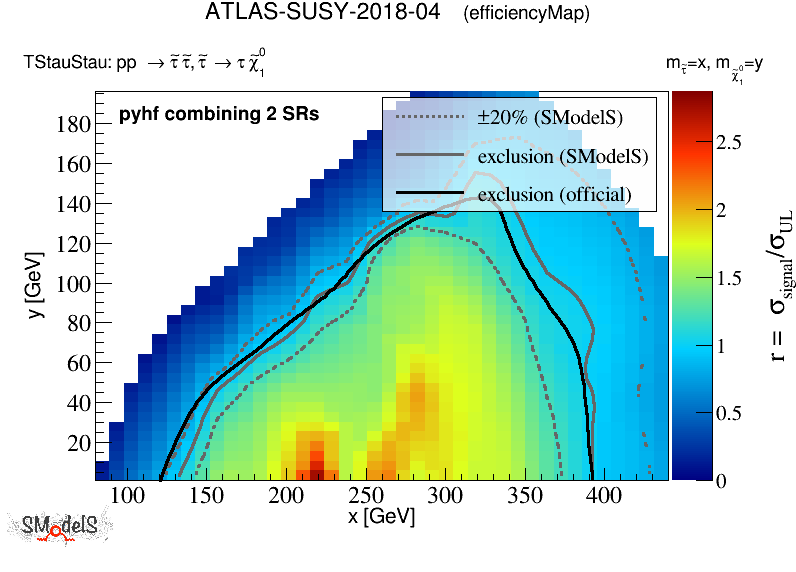
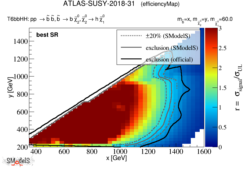
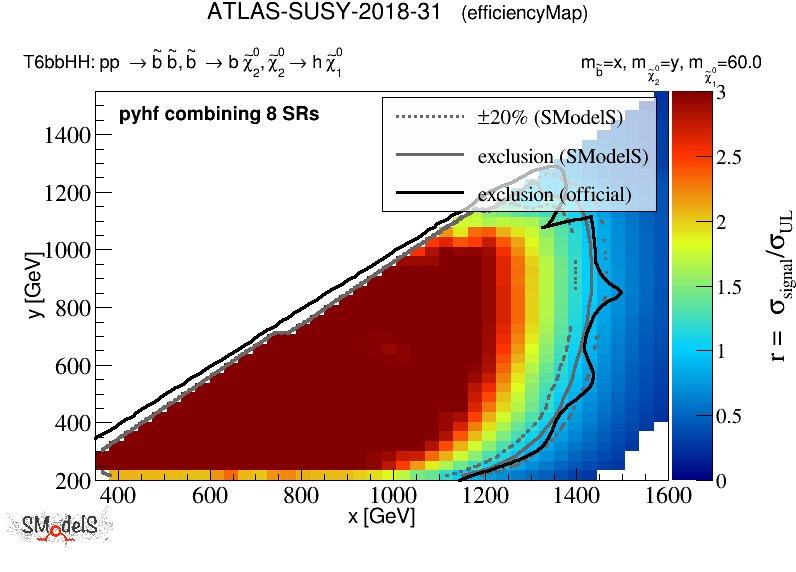
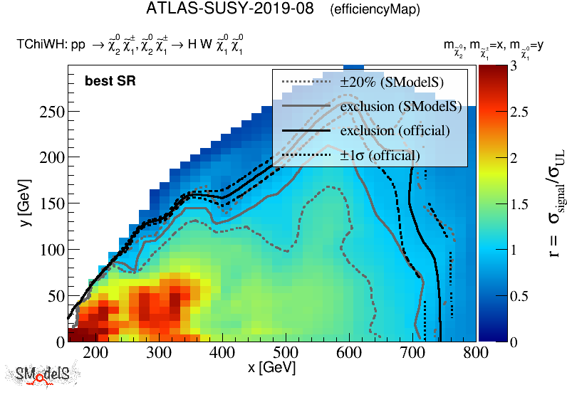
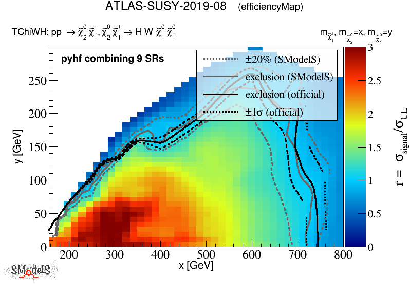
Even though we only show three results here, one can appreciate the gain in accuracy one can reach with using pyhf and full likelihoods. The ATLAS collaboration is at the beginning of a huge effort to provide full statistical models for new analyses. The first analyses published already show how this can help theorists make more trustful reinterpretations. The importance of such likelihood information for, e.g., global fits, has also been emphasised in [2].

4 Conclusions

We presented an interface of SModelS to pyhf that enables the use of the full likelihoods provided by ATLAS in the form of pyhf JSON files. The SModelS database was extended by efficiency map results with the corresponding JSON files of three new ATLAS SUSY analyses [16, 17, 23] for full Run 2 luminosity (139 fb^-1).

The new version, SModelS v1.2.4, is publicly available from https://smodels.github.io/ and can readily be employed for physics studies. We congratulate ATLAS to the important move of making full likelihood information available in digital format and are looking forward to including more such data in future updates of SModelS.

This completes the work started in contribution 15 of [9] for SModelS; the MadAnalysis 5 interface to pyhf should become available in the upcoming MadAnalysis 5 v1.9 release.

Last but not least we note that the technical discussions with the pyhf team are handled via github’s issue tracking system, see e.g.  https://github.com/scikit-hep/pyhf/issues/620, and are thus transparent and open to all.

References

- [1] S. Kraml, et al., Searches for New Physics: Les Houches Recommendations for the Presentation of LHC Results, Eur. Phys. J. C 72 (2012) 1976. arXiv:1203.2489, doi:10.1140/epjc/s10052-012-1976-3.
- [2] W. Abdallah, et al., Reinterpretation of LHC Results for New Physics: Status and Recommendations after Run 2, SciPost Phys. 9 (2020) 22. arXiv:2003.07868, doi:10.21468/SciPostPhys.9.2.022.
- [3] P. Asadi, M. R. Buckley, A. DiFranzo, A. Monteux, D. Shih, Digging Deeper for New Physics in the LHC Data, JHEP 11 (2017) 194. arXiv:1707.05783, doi:10.1007/JHEP11(2017)194.
- [4] P. Athron, et al., Combined collider constraints on neutralinos and charginos, Eur. Phys. J. C 79 (5) (2019) 395. arXiv:1809.02097, doi:10.1140/epjc/s10052-019-6837-x.
- [5] CMS Collaboration, Simplified likelihood for the re-interpretation of public CMS results, Tech. Rep. CMS-NOTE-2017-001, CERN, Geneva, https://cds.cern.ch/record/2242860 (Jan 2017).
- [6] S. Kraml, S. Kulkarni, U. Laa, A. Lessa, W. Magerl, D. Proschofsky, W. Waltenberger, SModelS: a tool for interpreting simplified-model results from the LHC and its application to supersymmetry, Eur.Phys.J. C74 (2014) 2868. arXiv:1312.4175, doi:10.1140/epjc/s10052-014-2868-5.
- [7] F. Ambrogi, S. Kraml, S. Kulkarni, U. Laa, A. Lessa, V. Magerl, J. Sonneveld, M. Traub, W. Waltenberger, SModelS v1.1 user manual: Improving simplified model constraints with efficiency maps, Comput. Phys. Commun. 227 (2018) 72–98. arXiv:1701.06586, doi:10.1016/j.cpc.2018.02.007.
- [8] F. Ambrogi, et al., SModelS v1.2: long-lived particles, combination of signal regions, and other novelties, Comput. Phys. Commun. 251 (2020) 106848. arXiv:1811.10624, doi:10.1016/j.cpc.2019.07.013.
- [9] G. Brooijmans, et al., Les Houches 2019 Physics at TeV Colliders: New Physics Working Group Report, in: 11th Les Houches Workshop on Physics at TeV Colliders: PhysTeV Les Houches, 2020. arXiv:2002.12220.
- [10] A. Buckley, M. Citron, S. Fichet, S. Kraml, W. Waltenberger, N. Wardle, The Simplified Likelihood Framework, JHEP 04 (2019) 064. arXiv:1809.05548, doi:10.1007/JHEP04(2019)064.
- [11] ATLAS Collaboration, Reproducing searches for new physics with the ATLAS experiment through publication of full statistical likelihoods, Tech. Rep. ATL-PHYS-PUB-2019-029, CERN, Geneva, https://cds.cern.ch/record/2684863 (Aug 2019).
- [12] K. Cranmer, G. Lewis, L. Moneta, A. Shibata, W. Verkerke, HistFactory: A tool for creating statistical models for use with RooFit and RooStats (CERN-OPEN-2012-016), https://cds.cern.ch/record/1456844.
- [13] L. Heinrich, M. Feickert, G. Stark, scikit-hep/pyhf, https://github.com/scikit-hep/pyhf, DOI: 10.5281/zenodo.1169739. doi:10.5281/zenodo.1169739.
- [14] J. Dutta, S. Kraml, A. Lessa, W. Waltenberger, SModelS extension with the CMS supersymmetry search results from Run 2, LHEP 1 (1) (2018) 5–12. arXiv:1803.02204, doi:10.31526/LHEP.1.2018.02.
- [15] C. K. Khosa, S. Kraml, A. Lessa, P. Neuhuber, W. Waltenberger, SModelS database update v1.2.3, to appear in LHEP. arXiv:2005.00555.
- [16] G. Aad, et al., Search for direct stau production in events with two hadronic -leptons in TeV collisions with the ATLAS detector, Phys. Rev. D 101 (3) (2020) 032009. arXiv:1911.06660, doi:10.1103/PhysRevD.101.032009.
- [17] G. Aad, et al., Search for bottom-squark pair production with the ATLAS detector in final states containing Higgs bosons, -jets and missing transverse momentum, JHEP 12 (2019) 060, HEPData entry: https://doi.org/10.17182/hepdata.89408. arXiv:1908.03122, doi:10.1007/JHEP12(2019)060.
- [18] F. Pezoa, J. L. Reutter, F. Suarez, M. Ugarte, D. Vrgoč, Foundations of json schema, in: Proceedings of the 25th International Conference on World Wide Web, International World Wide Web Conferences Steering Committee, 2016, pp. 263–273.
-
[19]
S. Kögl, jsonpatch
(6 2020).
URL https://github.com/stefankoegl/python-json-patch - [20] A. L. Read, Presentation of search results: The CL(s) technique, J. Phys. G 28 (2002) 2693–2704. doi:10.1088/0954-3899/28/10/313.
[21]
G. Cowan, K. Cranmer, E. Gross, O. Vitells,
Asymptotic formulae
for likelihood-based tests of new physics, The European Physical Journal C
71 (2).
doi:10.1140/epjc/s10052-011-1554-0.
URL http://dx.doi.org/10.1140/epjc/s10052-011-1554-0 - [22] P. Virtanen, R. Gommers, T. E. Oliphant, et al., SciPy 1.0: Fundamental Algorithms for Scientific Computing in Python, Nature Methods 17 (2020) 261–272. doi:https://doi.org/10.1038/s41592-019-0686-2.
- [23] G. Aad, et al., Search for direct production of electroweakinos in final states with one lepton, missing transverse momentum and a Higgs boson decaying into two -jets in (pp) collisions at TeV with the ATLAS detector, Eur. Phys. J. C 80 (8) (2020) 691, HEPData entry: https://doi.org/10.17182/hepdata.90607.v2. arXiv:1909.09226.