Private Weighted Random Walk Stochastic Gradient Descent

Abstract

We consider a decentralized learning setting in which data is distributed over nodes in a graph. The goal is to learn a global model on the distributed data without involving any central entity that needs to be trusted. While gossip-based stochastic gradient descent (SGD) can be used to achieve this learning objective, it incurs high communication and computation costs. To speed up the convergence, we propose instead to study random walk based SGD in which a global model is updated based on a random walk on the graph. We propose two algorithms based on two types of random walks that achieve, in a decentralized way, uniform sampling and importance sampling of the data. We provide a non-asymptotic analysis on the rate of convergence, taking into account the constants related to the data and the graph. Our numerical results show that the weighted random walk based algorithm has a better performance for high-variance data. Moreover, we propose a privacy-preserving random walk algorithm that achieves local differential privacy based on a Gamma noise mechanism that we propose. We also give numerical results on the convergence of this algorithm and show that it outperforms additive Laplace-based privacy mechanisms.

I Introduction

We consider the problem of designing a decentralized learning algorithm on data that is distributed among the nodes of a graph. Each node in the graph has some local data, and we want to learn a model by minimizing an empirical loss function on the collective data. We focus on applications such as decentralized federated learning or Internet-Of-Things (IoT) networks, where the nodes, being phones or IoT devices, have limited communication and energy resources. A crucial constraint that we impose is excluding the reliance on any central unit (parameter server, aggregator, etc.) that can communicate with all the nodes and orchestrate the learning algorithm. Therefore, we seek decentralized algorithms that are based only on local communication between neighboring nodes. Privacy is our main motivation for such algorithms since nodes do not have to trust a central unit. Naturally, decentralized algorithms come with the added benefits of avoiding single points of failure and easily adapting to dynamic graphs.

Gossip-style gradient descent algorithms, e.g.,[1], are a major contender for solving our problem. In Gossip algorithms, each node has a local model that is updated and exchanged with the neighboring nodes in each iteration. Gossip algorithms can be efficient time-wise since nodes can update their model in parallel. However, it incur high communication and energy (battery) cost in order to wait for all the local models to converge. This diminishes the appeal of Gossip algorithms for the applications we have in mind. Instead, we propose to study decentralized algorithms based on random walks. A random walk passes around a global model, and in each iteration, activates a node which updates the global model based on its local data. The activated node then passes the updated global model to a randomly chosen neighbor. The random walk guarantees that every cost spent on the communication and computation resources goes to improve the global model. Therefore, it outperforms Gossip algorithms in terms of these costs. In this paper, we will study how the design of the random walk affects the convergence of the learning algorithm. Namely, we propose two algorithms that we call Uniform Random Walk SGD and Weighted Random Walk SGD and study their convergence. Moreover, we consider the setting in which nodes do not completely trust their neighbors and devise locally differential variants of these algorithms.

I-A Previous work

The two works that are most related to our work are [2] and [3]. The work in [2] studies the random walk data sampling for stochastic gradient descent (SGD). The work of [3] focuses on importance sampling to speed up the convergence; however, it is implemented for a centralized setting.

A line of work on random walk based decentralized algorithm has been studied in the literature under the name of incremental methods. Early works on incremental methods by [4, 5, 6] have established theoretical convergence guarantees for different convex problem settings and using first-order methods of stochastic gradient updates. In [7], more advanced stochastic updates is been employed, namely CIAG [8], to improve the convergence guarantees for strongly convex objective by implementing unbiased total gradient tracking technique that uses Hessian information to accelerate convergence; they show that their algorithm converges linearly with high probability. The work of [2] proposed to speed-up the convergence by using non-reversible random walks. In [9], the authors studied the convergence analysis of random walk learning algorithm for the alternating direction method of multipliers (ADMM).

Gossip-based algorithms are also popular approach that has been widely studied, with application to averaging [10] and various stochastic gradient learning [6, 11, 12, 13] .

In terms of privacy, many works study differential privacy mechanisms for SGD algorithms. One approach for privacy is local differential privacy (LDP) [14, 15], where privacy is applied locally, which is well-suited for decentralized algorithms. Privacy mechanisms for SGD suggest protecting the output of every iteration by output perturbation [16] or by gradient perturbation and quantization (e.g.,[17, 18, 19, 20]).

I-B Contributions

In our work, we are interested in decentralized settings where the nodes have limited computation and communication power. Moreover, we assume that the nodes do not fully trust each others with their data and require privacy guarantees. For these reasons, we focus on first-order methods where the information exchanged between neighboring nodes is restricted to the model at a given iteration, serving both our communication and privacy constraints. Moreover, the update step involves only the gradient of the local loss function but no higher order derivatives, limiting the computation cost at the nodes. In this constrained setting, we study the design the random walk to speed up the convergence by simulating importance sampling.

It is known that the natural random walk on the vertices of a graph that picks one of the neighbors uniformly at random, will end up visiting nodes proportionally to their degree. The consequence of this is that the underlying SGD learning algorithm will be effectively sampling with higher probability the data on highly connected nodes. This sampling, which is biased by the graph topology, may or may not be a good choice for speeding-up the convergence of the algorithm, depending on which nodes have the important data.

We propose two alternate Markov-Hasting sampling schemes to address this bias, and study the convergence of the resulting algorithms: (i) Uniform Random Walk SGD (Algorithm 1), in which all the nodes are visited equally likely in the stationary regime irrespective of the node degrees. This emulates uniform data sampling in the centralized case ; (ii) The Weighted Random Walk SGD (Algorithm 2), in which the nodes are sampled proportional to the gradient-Lipschitz constant of their local loss function, rather than their degree. This emulates importance sampling [3, 21] in the centralized case.

We study the rate of convergence of both algorithms. The asymptotic rate of convergence of both algorithms is same as that of the natural random walk, namely, $\mathcal{O}(\frac{1}{k^{1-q}})$, where $k$ is the number of iterations and $q\in(\frac{1}{2},\,1)$. However, the constants are different and depend on the gradient-Lipschitz constants of the local loss functions and the graph spectral properties. Our numerical simulations highlight how these constants affect the non-asymptotic behavior of these algorithms. we observe that in high variance data regime Algorithm 2 outperforms Algorithm 1, and the opposite happens in a low variance data regime. These observations are in conformity with the behavior of importance sampling in [3] for the centralized case. This is expected since the random walks were designed to achieve, in the stationary regime, the same sampling strategy of the centralized case. The challenge, however, is with the proof techniques, which build on the random walk learning results in [2] and importance sampling in [3].

In addition, we propose a third algorithm, Private Weighted Random Walk SGD (Algorithm 3), that ensures local differential privacy of the local data. We propose a privacy mechanism that uses Gamma noise and characterize the tradeoff between the noise level and the privacy level. We also give numerical results on the convergence of Algorithm 3 and show that it outperforms additive Laplace-based privacy mechanisms.

Parts of these results pertaining to Algorithms 1 and 2 have already appeared in a conference paper [22].

I-C Organization

The rest of the paper is organized as follows. We formulate the problem in Section II. We present Algorithm 1 and Algorithm 2 in Section III. We present the convergence result of both algorithms in Subsection III-C. In Section IV, we define the Gamma mechanism and propose a privacy-preserving version of Algorithm 2. Finally, we present numerical results of our algorithms in Section V. We conclude in Section IV. The proofs of the technical results are deferred to the appendices.

II Problem Description

II-A Problem Setting

Network Model: We consider a communication network represented by an undirected graph $\mathcal{G}(V,\,E)$ with $V=\left[N\right]:=\{1,\ldots,N\}$ is the set of nodes and $E\subseteq V\times V$ is the set of edges. Two nodes in $\mathcal{G}$ connected by an edge in $E$ can communicate and exchange information. We refer to such two nodes as neighbors. We denote the set of neighbors of a node $i\in V$ by $\mathcal{N}(i)$, and its degree by $\deg(i):=|\mathcal{N}(i)|$. We assume that the graph $\mathcal{G}$ is connected, i.e., there exits a path between any two nodes in $V$. Moreover, we assume the presence of a self-loop at every node, i.e, $\{(i,\,i)\,:\,i=1,\,2,\,...,\,N\}\subset E.$ We assume that the set $\mathcal{N}(i)$ does not contain $i$.

Data and Learning Objective: Each node $i\in[N]$ has a feature vector $x_{i}\in\mathcal{X}\subseteq\mathbb{R}^{d}$, where $\mathcal{X}$ is the feature space and $d$ is the number of features. Moreover, node $i$ has a label $y_{i}\in\mathbb{R}$ corresponding to $x_{i}$.

The objective is to learn a prediction function on the collective data distributed over all the nodes by learning a global model $w\in\mathcal{W}$, where $\mathcal{W}$ is a closed and bounded subset in $\mathbb{R}^{d}$. Thus, an optimal model $w^{*}$ solves

$$\underset{w\in\mathcal{W}}{\text{minimize}}\frac{1}{N}\stackrel{{\scriptstyle[}}{{i}}=1]{N}{\sum} f_{i}\left(w;\,x_{i},\,y_{i}\right),$$ (1)

where $f_{i}\left(.\right)$ is the local loss function at node $i$. We denote the global loss function on all the data by

$$f\left(w\right)=\frac{1}{N}\stackrel{{\scriptstyle[}}{{i}}=1]{N}{\sum}f_{i}\left(w;\,x_{i},\,y_{i}\right).$$

We will assume convexity and gradient-Lipschitzness of the local loss functions as described in Assumption 1.

Assumption 1.

The local loss function $f_{i}$ for each node $i\in V$ is a convex function on $\mathcal{W}\in\mathbb{R}^{d}$ and has an $L_{i}$-Lipschitz continuous gradient; that is, for any $w$, $w^{\prime}\in\mathcal{W}$, there exists a constant $L_{i}>0$ such that

$$\left\|\nabla f_{i}\left(w\right)-\nabla f_{i}\left(w^{\prime}\right)\right\|_{2}\leq L_{i}\left\|w-w^{\prime}\right\|_{2}.$$

To solve the optimization problem in (1), we perform an iterative stochastic gradient descent (SGD) method. At each iteration $k$, one random node $i$ in the network will perform a gradient descent update and project the result back into the feasible set $\mathcal{W}$ as follows:

$$w^{(k+1)}={\bf{\Pi}}_{\mathcal{W}}\left(w^{(k)}-\gamma^{(k)}\hat{\nabla}f\left(w^{(k)}\right)\right),$$ (2)

where $\gamma^{(k)}$ is the step size, $w^{(k)}$ is the global model update at iteration $k$, and $\hat{\nabla}f\left(w^{(k)}\right)$ is a gradient estimate of the global loss function $f(.)$ based on one node $i$ local data. For convergence guarantees [23], we use a decreasing step size that satisfies

$$\stackrel{{\scriptstyle[}}{{k}}=1]{\infty}{\sum}\gamma^{(k)}=+\infty,\,\,\,\,\,\,\,\text{and}\,\,\,\,\,\,\,\stackrel{{\scriptstyle[}}{{k}}=1]{\infty}{\sum}\ln k.{(\gamma^{(k)})}^{2}<+\infty.$$ (3)

In particular, we will take $\gamma^{(k)}=\frac{1}{k^{q}}\,$ for $\,0.5<q<1$ which satisfy the conditions in (3).

Our goal is to implement a decentralized algorithm based on a Markov random walk sampling decision on the graph $\mathcal{G}$ to solve the learning problem in (1) with privacy guarantees, as explained in the next two sections.

II-B Random Walk Learning Algorithm

We seek a decentralized algorithm that will learn the model $w^{*}$ without involving a central entity, and in which nodes exchange information only with their neighbors. Towards that goal, we design a random walk on $\mathcal{G}$ that activates the node that it visits to update the global model based on the local data of the activated node. The algorithm is initiated at one node picked uniformly at random to be activated at the first iteration to perform the update in (2). Afterwards, at every iteration $k=1,\,2,\,...\,$, the global model iterate $w^{(k)}$ is passed to a randomly chosen node $i^{(k)}\in V$ to update it using its local data. Given the connection constraint, at iteration $k$, the activated node $i^{(k)}$ is a neighbor node of the previously activated node $i^{(k-1)}$, i.e., $i^{(k)}\in\mathcal{N}(i^{(k-1)})$. The process above defines a random walk on $\mathcal{G}$ that we model by a Markov chain. The sequence of active nodes $i^{(k)}$ are the states of the Markov chain with state-space $V$ and transition matrix $P$ that inherits the same connection structure of the underlying connected graph $\mathcal{G}$. For convergence guarantees, we will make the next assumption:

Assumption 2.

The Markov chain $(i^{(k)})_{k\in\mathbb{N}}$ defined on the finite state space $V$ with homogeneous transition matrix $P$ is irreducible and aperiodic and has a stationary distribution $\pi$ on $V$.

The problem is to design the transition probabilities in $P$ to speed up the convergence of the decentralized algorithm by only using the local information available to the nodes, namely their degrees and Lipschitz constants.

II-C Local Differential Privacy

In addition to designing a decentralized random walk learning algorithm that speeds up convergence, we aim for a privacy-preserving algorithm to protect each node data from being revealed by any other node including its neighbors.

We adopt local differential privacy (LDP) [14, 15] as a privacy measure that is well-suited to our decentralized setting, since we excluded the involvement of any central aggregator that would coordinate the learning process. Accordingly, nodes will share a noisy version of the messages that needs to be exchanged with the neighbors in a way that ensures a desired level of privacy for the nodes’ local data.

Consider a message $M(x_{i})$ that is to be sent from node $i$ to one of its neighbors. $M$ is a function of the node’s local data $M:\mathcal{X}\rightarrow\mathbb{M}$, where $\mathbb{M}$ is the image space. Let $\mathcal{R}:\mathbb{M}\rightarrow Img\mathcal{R}$ be the privatization scheme that node $i$ will perform on the message to share. For any two possible data points $x_{i},\,x^{\prime}_{i}\in\mathcal{X}$ that could be owned by a node $i$, the $(\epsilon,\,\delta)$-LDP defined as follows:

Definition 1 (Local Differential Privacy [14]).

A randomization mechanism $\mathcal{R}$ is $(\epsilon,\,\delta)$-LDP, if for any $x_{i},\,x^{\prime}_{i}\in\mathcal{X}$ and for any $r\in{Img}\mathcal{R}$, we have

$$P\left(\mathcal{R}\left(M\left(x_{i}\right)\right)=r\right)\leq e^{\epsilon}P\left(\mathcal{R}\left(M\left(x^{\prime}_{i}\right)\right)=r\right)+\delta,$$ (4)

where $\epsilon\geq 0$ quantifies the privacy level, and $\delta\in[0,1]$ quantifies the allowed probability of violating the privacy bound [24, 25].

A drawback of LDP noising mechanisms is that it will affect the utility of the exchanged messages and, as a result, slow the convergence of decentralized learning algorithm. We propose an LDP mechanism based on Gamma noise that achieves an attractive tradeoff between privacy and convergence, and outperforms generic additive-noise (Gaussian or Laplace) LDP mechanisms.

For ease of reference, we summarize our notation in Table I.

$\mathcal{G}$	Graph representing the network
$N$	Total number of nodes in $\mathcal{G}$
$V$	Set of nodes in $\mathcal{G}$
$E$	Set of edges in $\mathcal{G}$
$\deg\left(i\right)$	Degree of node $i$
$x_{i}$	Data feature vector of node $i$
$y_{i}$	Data label of node $i$
$f_{i}$	Local loss function of node $i$
$L_{i}$	Gradient-Lipschitz constant of $f_{i}$
$f$	Global loss function
$w$	Data model
$w^{*}$	Data optimal model
$w^{\left(k\right)}$	Model update at iteration $k$
$\sup L$	Maximum gradient-Lipschitz constant
$\inf L$	Minimum gradient-Lipschitz constant
$\bar{L}$	Average gradient-Lipschitz constant: $\bar{L}=\frac{L_{1}+L_{2}+...+L_{N}}{N}$
$i^{\left(k\right)}$	Node visited at time $k$
$\epsilon$	Privacy level
$1-\delta$	Privacy confidence level
$\pi_{u}$	Stationary distribution for uniform random walk
$P_{u}$	Transition matrix for uniform random walk
$\pi_{w}$	Stationary distribution for weighted random walk
$P_{w}$	Transition matrix for weighted random walk
$\mathcal{R}\left(L_{i}\right)$	Noisy version of $L_{i}$, output of the privacy mechanism
$\pi_{w,\,\mathcal{R}}$	Stationary distribution for noisy (private) weighted random walk

TABLE I: Notation

III Decentralized Weighted Random Walk SGD

We focus in this section on the design of the random walk learning algorithm without the privacy constraint. To decide on the transition probabilities of the random walk, a natural choice would be to pick the next node uniformly at random from the neighbors of the current active node. This gives a stationary distribution $\pi$ proportional to the degree of each node, i.e, $\pi(i)\sim\deg(i)$. Therefore, Assumption 2 implies the fraction of time a node is activated is directly proportional to its degree [26] . The effect of this random walk on the learning algorithm is that, in the update step of (2) the data is sampled proportional to the degree of the node that is carrying it. This node degree biased sampling may not be a favorable choice for speeding up the convergence of our decentralized learning algorithm. To counterbalance this bias, we propose two alternate sampling schemes and study the convergence of the resulting algorithms.

1. Uniform Random Walk SGD, in which all the nodes are visited equally likely in the stationary regime irrespective of their degree. This guarantees that the data points are eventually sampled uniformly at random irrespective of the graph topology.

2. Weighted Random Walk SGD, in which the nodes are sampled proportional to the gradient-Lipschitz constant of their local loss function, rather than their degree. The motivation is to achieve importance sampling [3, 21] in a decentralized fashion.

III-A Uniform Random Walk SGD

The Uniform Random Walk SGD algorithm aims at sampling the data points held by the graph nodes uniformly at random, similarly to what is done in standard centralized SGD [27, 28, 29]. We achieve the uniform data sampling by designing a random walk with a transition matrix $P_{u}$ using only local node information, such that the chain converges to the stationary distribution $\pi_{u}$ such that

$$\pi_{u}\left(i\right)=\frac{1}{N},\,\,\,\,\,\ \forall i\in V.$$

We implement the Metropolis Hasting (MH) decision rule to design the transition probabilities, so the random walk converges to the desired stationary $\pi_{u}$ [26, 30, 2]. The MH rule can be described as follows:

1. At the $k^{th}$ step of the random walk, the active node $i^{(k)}$ selects uniformly at random one of its neighbors, say $j$, as a candidate to be the next active node. This selection gets accepted with probability

   $$a_{u}\left(i^{(k)},\,j\right)=\min\left(1,\,\frac{\deg\left(i^{(k)}\right)}{\deg\left(j\right)}\right).$$

   Upon the acceptance, we have $i^{(k+1)}=j$.

2. Otherwise, if the candidate node gets rejected, the random walk stays at the same node, i.e., $i^{(k+1)}=i^{(k)}$.

Therefore, the transition matrix $P_{u}$ is given by

$$P_{u}\left(i,\,j\right)=\begin{cases}\frac{1}{\deg\left(i\right)}\min\,\left\{1,\,\frac{\deg\left(i\right)}{\deg\left(j\right)}\right\}&j\neq i\>\text{ and }\,j\in\mathcal{N}\left(i\right),\\ 1-\sum_{j\in\mathcal{N}\left(i\right)}\frac{1}{\deg\left(i\right)}\min\,\left\{1,\,\frac{\deg\left(i\right)}{\deg\left(j\right)}\right\}&j=i,\,\text{ and }\\ 0&\text{ otherwise. }\end{cases}$$

This random walk does conform with Assumption 2 and it uses local information only. By the Ergodic theorem [26] the above random walk that converges to a uniform stationary distribution, samples all the states (nodes) uniformly at random on the long-term run.

The Uniform Random Walk SGD implements the uniform random walk through the MH rule above. And, once a node is activated it updates the global model based on (2).

Algorithm 1 Uniform Random Walk SGD

   Initialization: Initial node $i^{(1)}$ chosen uniformly at random from $[N]$, Initial model $w^{(1)}$ chosen uniformly at random from $\mathcal{W}$

  for $k=1$ to $T$ do

     $\hat{\nabla}f\left(w^{(k)}\right)={\nabla}f_{i}\left(w^{(k)}\right)$.

     $w^{(k+1)}={\bf{\Pi}}_{\mathcal{W}}\left(w^{(k)}-\gamma^{(k)}\hat{\nabla}f\left(w^{(k)}\right)\right)$

     Choose node $j$ uniformly at random from $\mathcal{N}\left(i^{(k)}\right).$

     Generate $p\sim U\left(0,\,1\right)$ where $U$ is the uniform distribution.

     if $p\leq\min\,\left\{1,\,\frac{\deg\left(i^{(k)}\right)}{\deg\left(j\right)}\right\}$ then

        $i^{(k+1)}\leftarrow j$

     else

        $i^{(k+1)}\leftarrow i^{(k)}$

     end if

  end for

  Return: $w^{(T)}.$

In subsection III-C, we give the convergence analysis for this algorithm.

III-B Weighted Random Walk SGD

To speed up the convergence, we propose a decentralized sampling that mimics centralized importance sampling, which consists of selecting more often the more informative data points [3, 21, 31, 32, 33, 34]. In our our analysis, we will take the data importance to be reflected through the gradient-Lipschitz constant of the node’s local loss function [3]. Again, we utilize the MH decision rule for the random walk to achieve a stationary distribution proportional to the node gradient-Lipschitz constant as follows

$$\pi_{w}\left(i\right)=\frac{L_{i}}{\sum_{j=1}^{N}L_{j}}\,\,\,\,\,\ \forall i\in V.$$

The random walk proceeds as previously explained, except for the probability of accepting the candidate node, which is now

$$a_{w}\left(i^{(k)},\,j\right)=\min\left(1,\,\frac{L_{j}}{L_{i^{(k)}}}\frac{\deg\left(i^{(k)}\right)}{\deg\left(j\right)}\right).$$ (5)

Consequently, the new transition matrix $P_{w}$ generating the weighted random walk is given by

$$P_{w}\left(i,\,j\right)=\begin{cases}\frac{1}{\deg\left(i\right)}\min\,\left\{1,\,\frac{L_{j}}{L_{i}}\frac{\deg\left(i\right)}{\deg\left(j\right)}\right\}&j\neq i\>\text{and}\,j\in\mathcal{N}\left(i\right),\\ 1-\sum_{j\in\mathcal{N}\left(i\right)}\frac{1}{\deg\left(i\right)}\min\,\left\{1,\,\frac{L_{j}}{L_{i}}\frac{\deg\left(i\right)}{\deg\left(j\right)}\right\}&j=i,\,\text{and}\\ 0&\text{otherwise}.\end{cases}$$

Algorithm 2 Weighted Random Walk SGD

   Initialization: Initial node $i^{(1)}$ chosen uniformly at random from $[N]$, Initial model $w^{(1)}$ chosen uniformly at random from $\mathcal{W}$

  Every node $i$ shares $L_{i}$ and $\deg(i)$ it with its neighbors.

  for $k=1$ to $T$ do

     $\hat{\nabla}f\left(w^{(k)}\right)={\frac{\bar{L}}{L_{i^{(k)}}}}{\nabla}f_{i^{(k)}}\left(w^{(k)}\right)$

     $w^{(k+1)}={\bf{\Pi}}_{\mathcal{W}}\left(w^{(k)}-{\gamma^{(k)}}\hat{\nabla}f\left(w^{(k)}\right)\right)$

     Choose node $j$ uniformly at random from $\mathcal{N}\left(i^{(k)}\right).$

     Generate $p\sim U\left(0,\,1\right)$ where $U$ is the uniform distribution.

     if $p\leq\min\,\left\{1,\,\frac{L_{j}}{L_{i^{(k)}}}\frac{\deg\left(i^{(k)}\right)}{\deg\left(j\right)}\right\}$ then

        $i^{(k+1)}\leftarrow j$

     else

        $i^{(k+1)}\leftarrow i^{(k)}$

     end if

  end for

  Return: $w^{(T)}.$

III-C Convergence Analysis

We summarize here our main results on the convergence of Algorithms 1 and 2. Our aim is to characterize how the design of the random walk affects the non-asymptotic rate of convergence of the algorithms. To give a bit of context, for convex and gradient-Lispchitz objective functions, centralized SGD has an asymptotic convergence rate in the order of $\mathcal{O}(\frac{1}{\sqrt{k}})$ (after $k$ iterations) for diminishing step-size and for independent data sampling [35, 36]. For our decentralized setting, in which data sampling is not independent and is constrained by the graph topology, random walk SGD algorithms can approach the same rate of convergence for convex global loss function [37, 2, 4, 5, 1]. Namely, for a step-size $\gamma^{(k)}=\frac{1}{k^{q}}$ with $\frac{1}{2},<q<1$, the work in [2] proves a rate of convergence $\mathcal{O}(\frac{1}{k^{1-q}})$.

It was shown in [37] that $\Omega(\frac{1}{\sqrt{k}})$, $k$ being the number of SGD updates, is a fundamental lower bound on the convergence rate for convex optimization within the stochastic first-order oracle model with no access to independent sampling.

Our proposed algorithms will also have this rate of convergence. However, the choice of the random walk will affect the constants in the rate of convergence and can lead to a speed-up in the non-asymptotic regime. Theorems 1 and  2 characterize these constants of our proposed algorithms.

We denote the eigenvalues of any the transition matrix $P$ of the random walk by $\lambda_{1}=1>\lambda_{2}\geq...\geq\lambda_{N}$, and define $\lambda_{P}=\frac{\underset{}{\max}{\left\{\left|\lambda_{2}\right|,\left|\,\lambda_{N}\right|\right\}}+1}{2}.$

Theorem 1 (Convergence of Algorithm 1).

Under Assumptions 1 and  2, the Uniform Random Walk SGD (Algorithm 1) converges in the mean sense, i.e.,

$$\underset{k\rightarrow\infty}{\lim\,}\mathbb{E}\left(f\left(w^{(k)}\right)-f\left(w^{*}\right)\right)=0.$$ (6)

Moreover, its rate of convergence, for a step size $\gamma^{(k)}=\frac{1}{k^{q}}$, $0.5<q<1$, is

$$\mathbb{E}\left[f\left(\bar{w}^{(k)}\right)-f\left(w^{*}\right)\right]=O\left(\frac{\max\left\{\sigma^{2},\,\left(\sup L\right)^{2},\,\frac{1}{\ln\left(1/\lambda_{P_{u}}\right)}\right\}}{k^{1-q}}\right),$$ (7)

where, $\bar{w}^{(k)}=\frac{1}{\stackrel{{\scriptstyle[}}{{n}}=1]{k}{\sum}\gamma^{(n)}}\stackrel{{\scriptstyle[}}{{m}}=1]{k}{\sum}\gamma^{(m)}w^{(m)}$, $\sup L=\underset{i\in V}{\max}L_{i}$ and the residual $\sigma^{2}=\underset{w^{*}}{\max}\,\mathbb{E}\left[\left\|\nabla f_{i}\left(w^{*}\right)\right\|_{2}^{2}\right]$.

Note the technicality that the convergence is in terms of $\bar{w}^{(k)}$, instead of $w^{(k)}$, which is weighted average of the $w^{(k)}$s. This is due to the proof technique. Next, we give the bound on the convergence rate for the Weighted Random Walk SGD.

Theorem 2 (Convergence rate of Algorithm 2).

Under assumptions 1 and  2, the Weighted Random Walk SGD (Algorithm 2) converges in the mean sense, i.e.,

$$\underset{k\rightarrow\infty}{\lim\,}\mathbb{E}\left(f\left(w^{(k)}\right)-f\left(w^{*}\right)\right)=0.$$ (8)

Moreover, its rate of convergence, for a step size $\gamma^{(k)}=\frac{1}{k^{q}}$ when $0.5<q<1$, is

$$\mathbb{E}\left[f\left(\bar{w}^{(k)}\right)-f\left(w^{*}\right)\right]=O\left(\frac{\max\left\{\frac{\bar{L}}{\inf L}\sigma^{2},\,\left(\bar{{L}}\right)^{2},\,\frac{1}{\ln(1/\lambda_{P_{w}})}\right\}}{k^{1-q}}\right),$$ (9)

where $\inf L=\underset{i\in V}{\min}\,L_{i}$ and $\bar{L}=\frac{\sum_{i}L_{i}}{N}$.

The results on the rate of convergence stated in the above theorems show the tradeoff that the two random walks offer. The weighted sampling for random walk SGD improves the bound on convergence from being a function of $\sup L$ to be a function of the average $\bar{L}$. However, it amplifies the effect of the residual represented by $\sigma^{2}$. The numerical results will show later that in high variance data regime resulting in a wide range for the values of the Lipschitz constants, the improvement brought by $\bar{L}$ dominates over the residual amplification, so Algorithm 2 outperforms Algorithm 1. However, the opposite happens for a low variance data regime where the data variance is low, and therefore the gap between $\sup L$ and $\bar{L}$ is not significant. Therefore, these observations are in conformity with the behavior of importance sampling in [3] for the centralized case. The proof of Theorem 1 follows the same steps as in [2] with incorporation of the Lipschitzness assumption and we provide it for completeness and for comparison with Theorem 2. The detailed proofs for both theorems can be found in Appendices A and B.

III-D Comparison to Gossip Algorithm:

To better understand the performance of our two algorithms, we compare them to Gossip algorithm. One of the most common approaches of the Gossip algorithms is the synchronous version [6, 38, 39, 40, 31], in which at every round, all nodes exchange and update their local models. For convex problems, the convergence rate is $O(1/\sqrt{k})$ [41], where $k$ is the algorithm round in which $|\mathcal{E}|$ communication links are activated and $O(N)$ computations are performed. Therefore, the convergence rate as function of communication cost is $O({|\mathcal{E}|}/{\sqrt{k}})$, and as a function of computation cost is $O({N}/{\sqrt{k}})$. However, the convergence rate of Algorithms  1 and 2 as a function of computation and communication cost approaches a rate of $O(1/\sqrt{k})$. That is because at each round at most one communication link is activated and one SGD update is performed.

IV Differential private Random Walk SGD

In this section, we propose an LDP mechanism to be applied to the messages exchanged within Algorithm 2 to make it privacy-preserving. Algorithm 2 requires sharing two pieces of information between two neighbouring nodes:

1. The gradient-Lipschitz constants: Algorithm 2 requires every node $i\in V$ to share the gradient-Lipschitz constant $L_{i}$ with all its neighbors to be able to implement the MH rule of (5). This can leak important information about the local data at the nodes. For instance, for linear regression loss function, we have $L_{i}=N\|x_{i}\|^{2}_{2}$.

2. The model updates: An activated node needs to receive the latest updated version of the model $w^{(k)}$, which naturally contains information about the data on the nodes visited so far.

The literature on privacy-preserving SGD has extensively studied the problem of designing LDP mechanisms for the model update or the gradient through model perturbation (e.g., [16]) or gradient perturbation and quantization (e.g.,[17, 18, 19, 20]). Within that space of works, the new aspect of our problem is the sharing of the gradient-Lipschitz constants. For this reason, we focus in our analysis on characterizing how sharing privatized (noisy) versions of these constants would affect the random walk learning algorithm, and assume that the models are shared in the clear.

We propose Algorithm 3 which is a modification of Algorithm 2 that makes it privacy-preserving by adding an LDP mechanism on the gradient-Lipschitz constants. We define this mechanism below and refer to it as the Gamma mechanism.

Definition 2 (Gamma mechanism).

The Gamma mechanism takes as input the gradient-Lipschitz constant $L_{i}$ of node $i$ and outputs

$$\mathcal{R}(L_{i})\sim{{Gamma}}(\frac{L_{i}}{\theta},\,\theta),$$

where $\theta>0$ is a noise parameter that controls the privacy level.

As a reminder, the probability density function of a random variable $L$ distributed according to Gamma$(k,\theta)$ with a shape $k>0$ and scale $\theta>0$ is

$$p_{{G,L}}\left(l\right)=\frac{1}{\varGamma\left(k\right)\theta^{k}}l^{k-1}e^{-\frac{l}{\theta}},\text{ for }\,\,l>0,$$

where $\Gamma\left(z\right)=\int_{0}^{\infty}u^{z-1}e^{-u}du\text{\,\,\,\,for\,\,\,\,}z>0.$

If $k$ is an integer, the Gamma distribution can be interpreted as the sum of $k$ exponential random variable with mean $\theta$ [42]. Computing the mean and the variance of $\mathcal{R}(L_{i})$, we get the mean $\mathbb{E}_{\mathcal{R}}\left[\mathcal{R}(L_{i})\right]=\frac{L_{i}}{\theta}\theta=L_{i},$ and the variance $v_{\mathcal{R}}\left[\mathcal{R}(L_{i})\right]=L_{i}\theta$ and thus $\theta$ determines the noise level in the Gamma mechanism.

Accordingly, we obtain Algorithm 3 that we call Private Weighted Random Walk SGD:

Algorithm 3 Private Weighted Random Walk SGD

   Initialization: Initial node $i^{(1)}$ chosen uniformly at random from $[N]$, Initial model $w^{(1)}$ chosen uniformly at random from $\mathcal{W}$.

  Every node $i$ computes $\mathcal{R}(L_{i})$ and shares it along with $\deg(i)$ with its neighbors.

  for $k=1$ to $T$ do

     $\hat{\nabla}f\left(w^{(k)}\right)={\frac{\bar{L}}{L_{i^{(k)}}}}{\nabla}f_{i^{(k)}}\left(w^{(k)}\right)$

     $w^{(k+1)}={\bf{\Pi}}_{\mathcal{W}}\left(w^{(k)}-{\gamma^{(k)}}\hat{\nabla}f\left(w^{(k)}\right)\right)$

     Choose node $j$ uniformly at random from $\mathcal{N}\left(i^{(k)}\right).$

     Generate $p\sim U\left(0,\,1\right)$ where $U$ is the uniform distribution.

     if $p\leq\min\,\left\{1,\,\frac{\mathcal{R}({L}_{j})}{\mathcal{R}({L}_{i^{(k)}})}\frac{\deg\left(i^{(k)}\right)}{\deg\left(j\right)}\right\}$ then

        $i^{(k+1)}\leftarrow j$

     else

        $i^{(k+1)}\leftarrow i^{(k)}$

     end if

  end for

  Return: $w^{(T)}.$

In this algorithm, each node $i$ applies the Gamma mechanism to its constant $L_{i}$ only once and shares $\mathcal{R}(L_{i})$ with its neighbors before the start of the random walk. These fixed values $\mathcal{R}(L_{i})$’s are then used throughout the algorithm. The stationary distribution of the weighted random walk of Algorithm 3 with the noisy values $\mathcal{R}(L_{i})$ is

$$\pi_{w,\mathcal{R}}(i)=\frac{\mathcal{R}~{}\left(L_{i}\right)}{\sum_{j}\mathcal{R}\left(L_{j}\right)},$$

and it follows the Beta distribution [42], i.e., $\pi_{w,\mathcal{R}}(i)\sim\text{Beta}\left(\frac{L_{i}}{\theta},\,\frac{\sum_{j\neq i}L_{j}}{\theta}\right).$ Note that the probability density function of the Beta distribution of a random variable $\Pi$, with parameters $\alpha,\,\beta>0$ is

$$p_{B,\Pi}(\pi)=\frac{\pi^{\alpha-1}\left(1-\pi\right)^{\beta-1}}{B\left(\alpha,\,\beta\right)},\quad\text{for\,}\pi\in\left[0,\,1\right],$$

where $B\left(\alpha,\,\beta\right)=\frac{\Gamma\left(\alpha\right)\Gamma\left(\beta\right)}{\Gamma\left(\alpha+\beta\right)}.$

Therefore, we get that the mean of $\pi_{w,\,\mathcal{R}}$ over the privatization randomness is the desired stationary distribution of importance sampling, i.e,

$$\mathbb{E}_{\mathcal{R}}\left[\pi_{w,\,\mathcal{R}}\right]=\pi_{w}(i),\,\,\,\,\forall i\in V.$$

We can see that the Beta distribution is well fitted to model the probability distribution of a probability [43] where the expected values of the stationary probabilities sums $1$, which justifies our choice for the Gamma noise over other traditional additive privacy schemes (e.g., Gaussian, Laplace) since it implies a Beta distribution on the ratio representing the stationary distribution.

Moreover, this implies that the gradient estimate is unbiased at the stationary, that is

$$\mathbb{E}_{\mathcal{R}}\mathbb{E}_{\pi_{w,\,\mathcal{R}}}\left[\hat{\nabla}f_{i}\,|\,\mathcal{R}\left(L_{j}\right),\,j=1,\,...,\,N\right] =\nabla f,$$

the proof of which can be found in Appendix C.

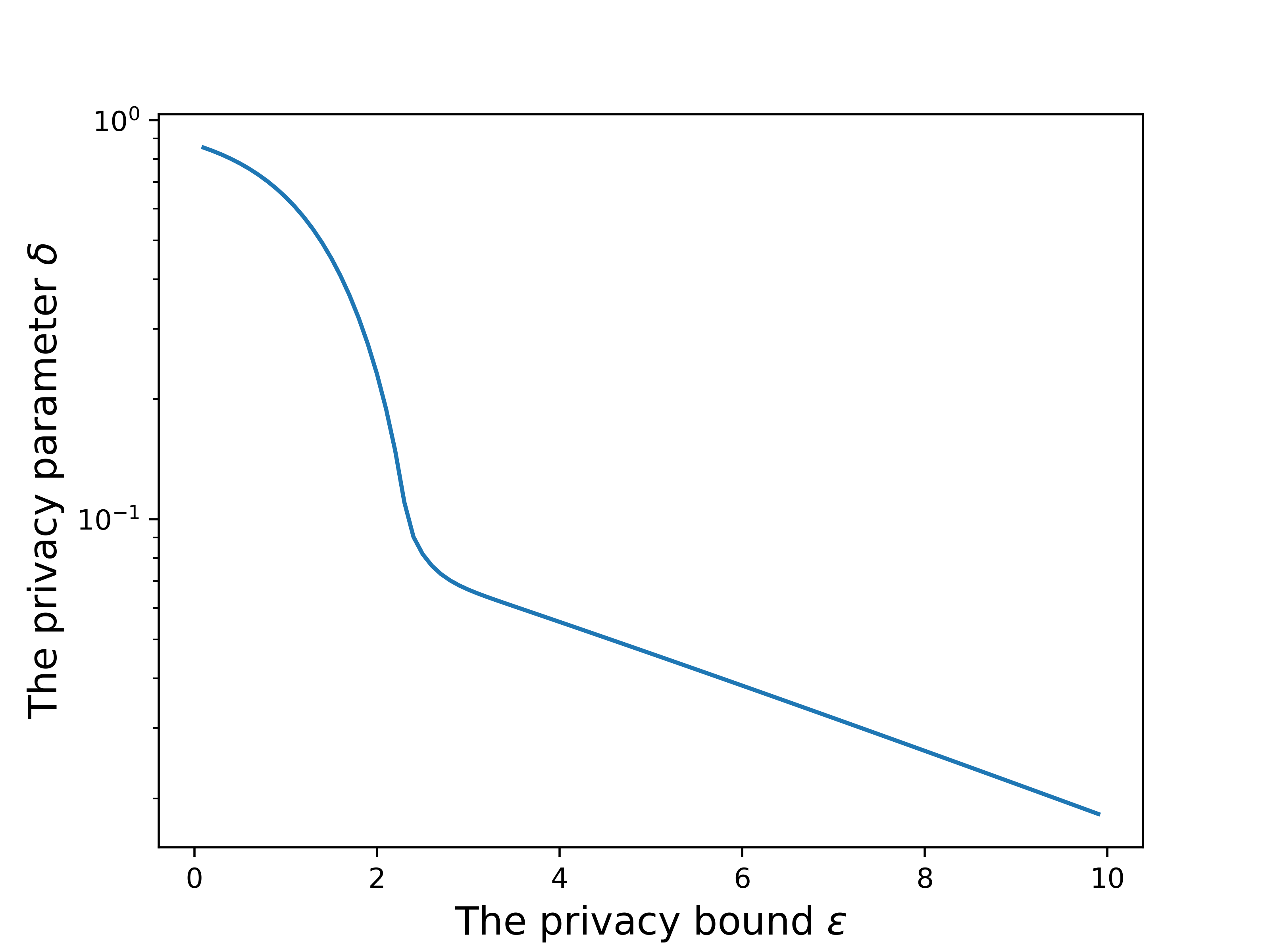
(a) The achievable privacy parameter $\delta$ as a function of the privacy bound $\epsilon$.

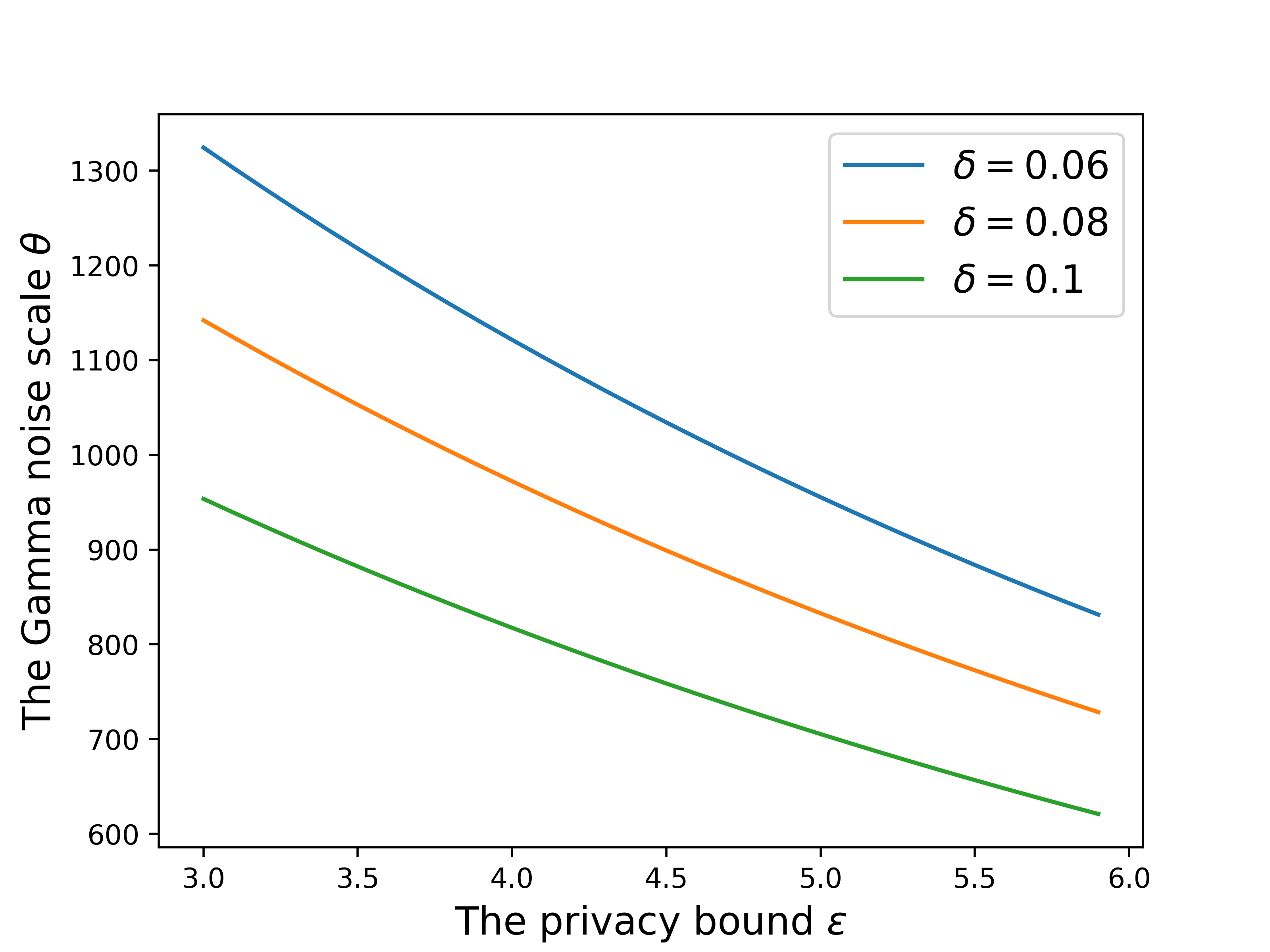
(b) The Gamma noise parameter $\theta$ vs. the privacy bound $\epsilon$ for $\delta=0.06,\,0.08\,\&\,0.1$.

Figure 1: The tradeoffs stated in Lemma 3 between the privacy level, quantified through $\epsilon$ and $\delta$, and the noise level represented by $\theta$ for the Gamma mechanism.

The next Lemma states the tradeoff between the privacy level, quantified through $\epsilon$ and $\delta$, and the noise level represented by $\theta$ for the Gamma mechanism.

Lemma 3.

Given $\epsilon\geq 0$ , the Gamma mechanism is $\left(\epsilon,\,\delta\right)$ local differential private with parameter $\theta$ satisfying

$$\delta\geq\max\left\{1-\frac{{IG}\left(\frac{\sup L}{\theta},\left(e^{\epsilon}\frac{\Gamma\left(\sup L/\theta\right)}{\Gamma\left(\inf L/\theta\right)}\right)^{\frac{\theta}{\sup L-\inf L}}\right)}{\Gamma\left(\sup L/\theta\right)},\frac{{IG}\left(\frac{\inf L}{\theta}\,,\,\left(\frac{1}{e^{\epsilon}}\frac{\Gamma\left(\sup L/\theta\right)}{\Gamma\left(\inf L/\theta\right)}\right)^{\frac{\theta}{\sup L-\inf L}}\right)}{\Gamma\left(\inf L/\theta\right)}\right\}$$

where $IG\left(s,t\right):=\int_{0}^{t}u^{s-1}e^{-u}du$ is the incomplete gamma function.

The proof of Lemma 3 is in Appendix D. In Fig. 1 shows plots of the tradeoff among the three parameters $\epsilon$, $\delta$ and $\theta$ descrbied in the above lemma.

Convergence Analysis: The proposed Gamma mechanism applies the Gamma noise to the gradient-Lipschitz constants $L_{i}$’s only one time before the start of the algorithm. Therefore, finding the expression of the rate of convergence in Algorithm 3, given the generated noisy Lipschitz constants $\mathcal{R}\left(L_{i}\right)$, follows similar steps as the analysis of non-private version of the algorithm and gives the following bound.

$$\mathbb{E}\left[f\left(\bar{w}^{(k)}\right)-f\left(w^{*}\right)|\,\mathcal{\mathcal{R}}\left(L_{i}\right),\,i=1,...,\,N\right]$$

$$=\mathcal{O}\left(\frac{\max\left\{\frac{\overline{\mathcal{\mathcal{R}}\left(L\right)}}{\inf\mathcal{\mathcal{R}}\left(L\right)}\sigma^{2},\,\left(\overline{\mathcal{\mathcal{R}}\left(L\right)}\right)^{2},\,\frac{1}{\ln 1/\lambda_{P_{w,\,\mathcal{R}}}}\right\}}{k^{1-q}}\right).$$ (10)

To characterize the mean rate of convergence under the Gamma mechanism we need to average the bound above over the noise introduced by the mechanism. This involves finding the mean of the different terms in the right-hand-side of (10), which is not straightforward given that the noise introduced by the Gamma mechanism is not additive. Instead, we analysis a modification of the mechanism that we call Truncated Gamma mechanism, which first implements the Gamma mechanism and then truncates the values $\mathcal{R}\left(L_{i}\right)$ to a minimum and maximum constants $L_{min}$ and $L_{max}$ ($L_{min}<L_{max}$). By Proposition 2.1 in [24] on the post-processing differential privacy immunity rule, we know that the Truncated Gamma mechanism achieves the privacy guarantees ($\epsilon,\delta$) of the non-truncated version and is more amenable to analysis as done below (as the expense of the tightness of the bound):

$$\mathbb{E}_{\mathcal{R}}\left[\mathbb{E}\left[f\left(\bar{w}^{(k)}\right)-f\left(w^{*}\right)\right]\right]=O\left(\frac{\frac{L_{max}}{L_{min}}\sigma^{2}+\left(L_{\max}\right)^{2}}{k^{1-q}}\right).$$ (11)

We can see that the bound in (11) benefits from the same asymptotic rate of convergence as the non-private version.

V Numerical Results

In this section, we present our numerical results applying Algorithms 1, 2 and 3 to a decentralized logistic regression problem and comparing it to asynchronous Gossip SGD algorithm [1]. We compare the Random Walk algorithms to the asynchronous Gossip to show the convergence speed-up with respect to the number of performed SGD iterations in the network. For fair comparison in terms of computation and communication, we assume an asynchronous Gossip algorithm where only one communication link gets activated at every iteration and the model on both side gets updated, exchanged and averaged. Also, we run Algorithm 3 using the LDP privatization scheme based on the Gamma mechanism, and we compare it to the additive Laplace mechanism widely used in the literature [24].

We take the graph $\mathcal{G}$ to be an Erdős-Rényi graph on $N=100$ nodes with probability of connectivity $p=0.3$. We assume that the labels $y_{i}\in\{-1,+1\}$. For the data with label $y_{i}=1$, we sample $x_{i}$ from $\mathcal{N}\left({{\mu}},v\,\mathbb{I}_{d}\right)$ where $d$ is the feature dimension, $\mu$ is the mean, $v$ is the variance and $\mathbb{I}_{d}$ is the identity matrix of dimension $d$. For label $y_{i}=-1$, $x_{i}$ is sampled from $\mathcal{N}\left(-{\mu},v\,\mathbb{I}_{d}\right)$.

Loss function: The averaged regularized cost function for logistic regression on the distributed data can be expressed as follow:

$$f\left(w\right)=\stackrel{{\scriptstyle[}}{{i}}=1]{N}{\sum}\log\left(1+\exp\left(-y_{i}x_{i}^{T}w\right)\right)+\frac{1}{2}\|w\|^{2}.$$ (12)

So, the local loss function at node $i$ is

$$f_{i}\left(w\right)=N\log\left(1+\exp\left(-y_{i}x_{i}^{T}w\right)\right)+\frac{N}{2}\|w\|^{2}.$$ (13)

Then, for such local loss function the gradient Lipschitz constant is $L_{i}=1+\frac{1}{4}N\left\|x_{i}\right\|_{2}^{2}$.

Random Walk algorithms vs the Gossip algorithm: We consider two data regimes for our simulations: High variance and Low variance regimes. For both regimes, the random walk based algorithms outperform the Gossip algorithm as shown in Figure 2. For the high variance data regime where $v=10$, the term $\bar{L}$ in the convergence rate dominates, and the weighted sampling gives better convergence. While in the low variance data regime where $v=1$, the Uniform Random Walk SGD is outperforming the Weighted Random Walk SGD.

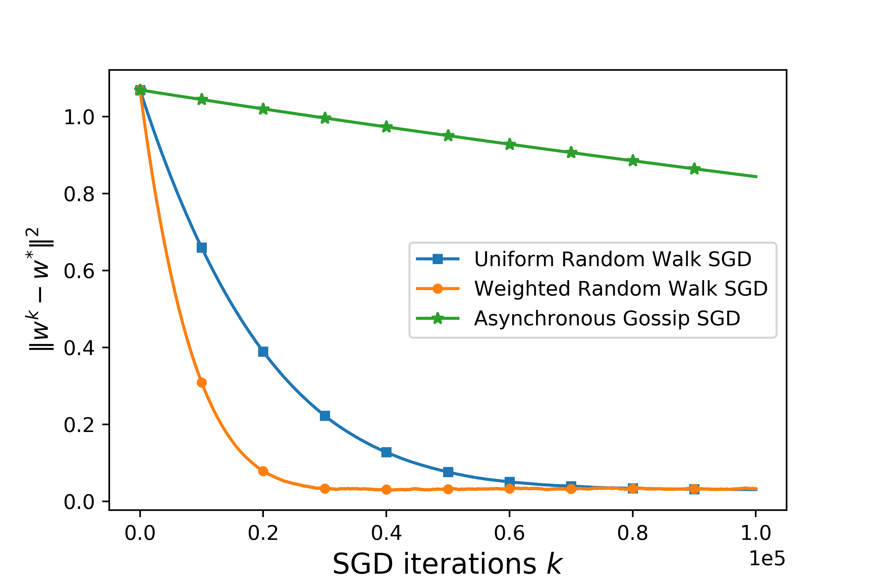
(a) High variance data regime: $v=10$.

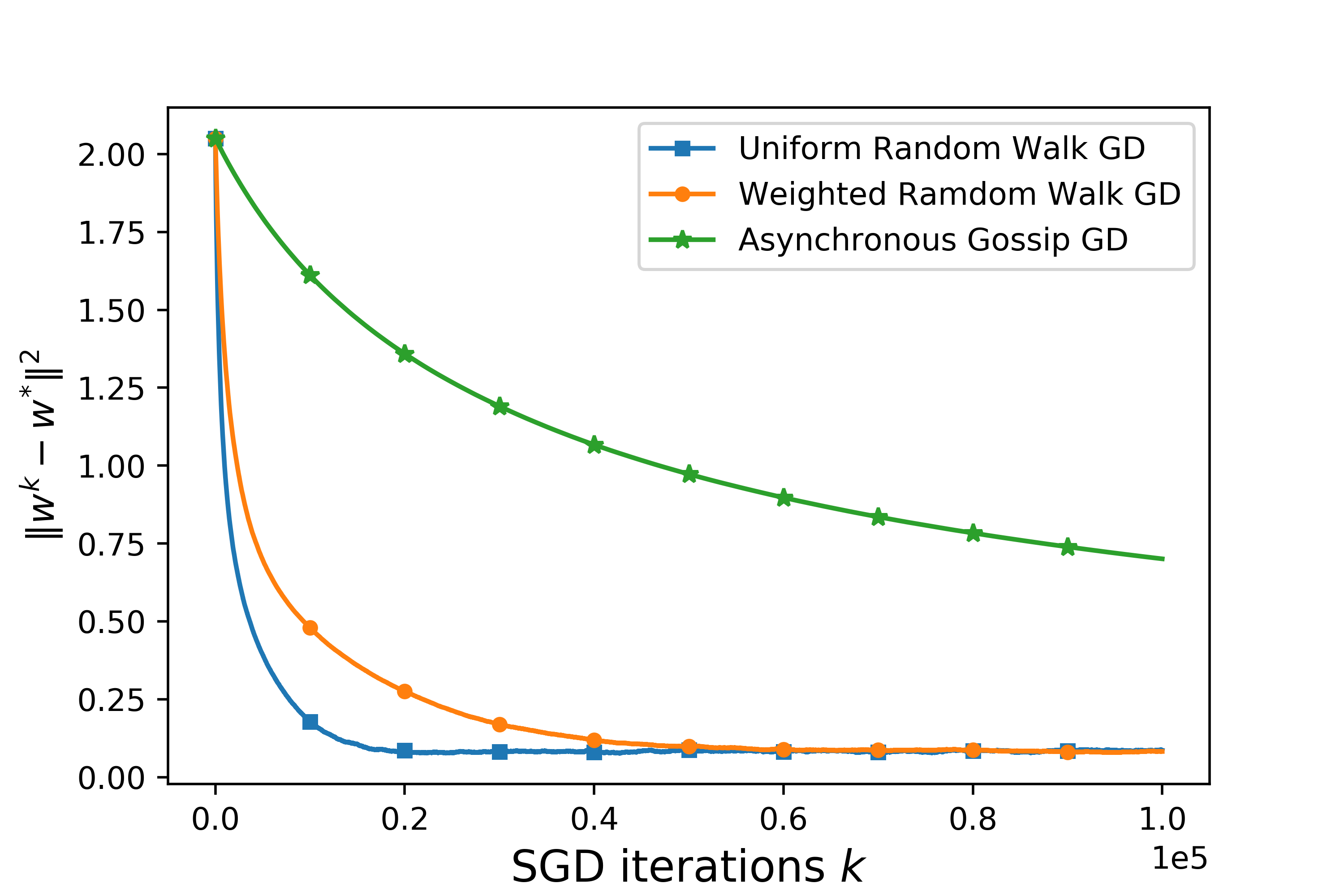
(b) Low variance data regime: $v=1$.

Figure 2: Error on the model function of the SGD updates estimated by the Uniform Random Walk SGD (Algorithm 1), Weighted Random Walk SGD (Algorithm 2) and the asynchronous Gossip SGD on an Erdős-Rényi graph of $100$ nodes and probability of connectivity $p=0.3$.

Private Random Walk algorithms: For high variance regime, we simulate the convergence of Algorithm 3 that used the Gamma mechanism. We compare its performance to a variant that uses an additive Laplacian noise, [24] for $\epsilon=3$ and $\delta\leq 0.03$ with same noise variance as the Gamma. Our results show that the Gamma mechanism outperforms the Laplacian mechanism .

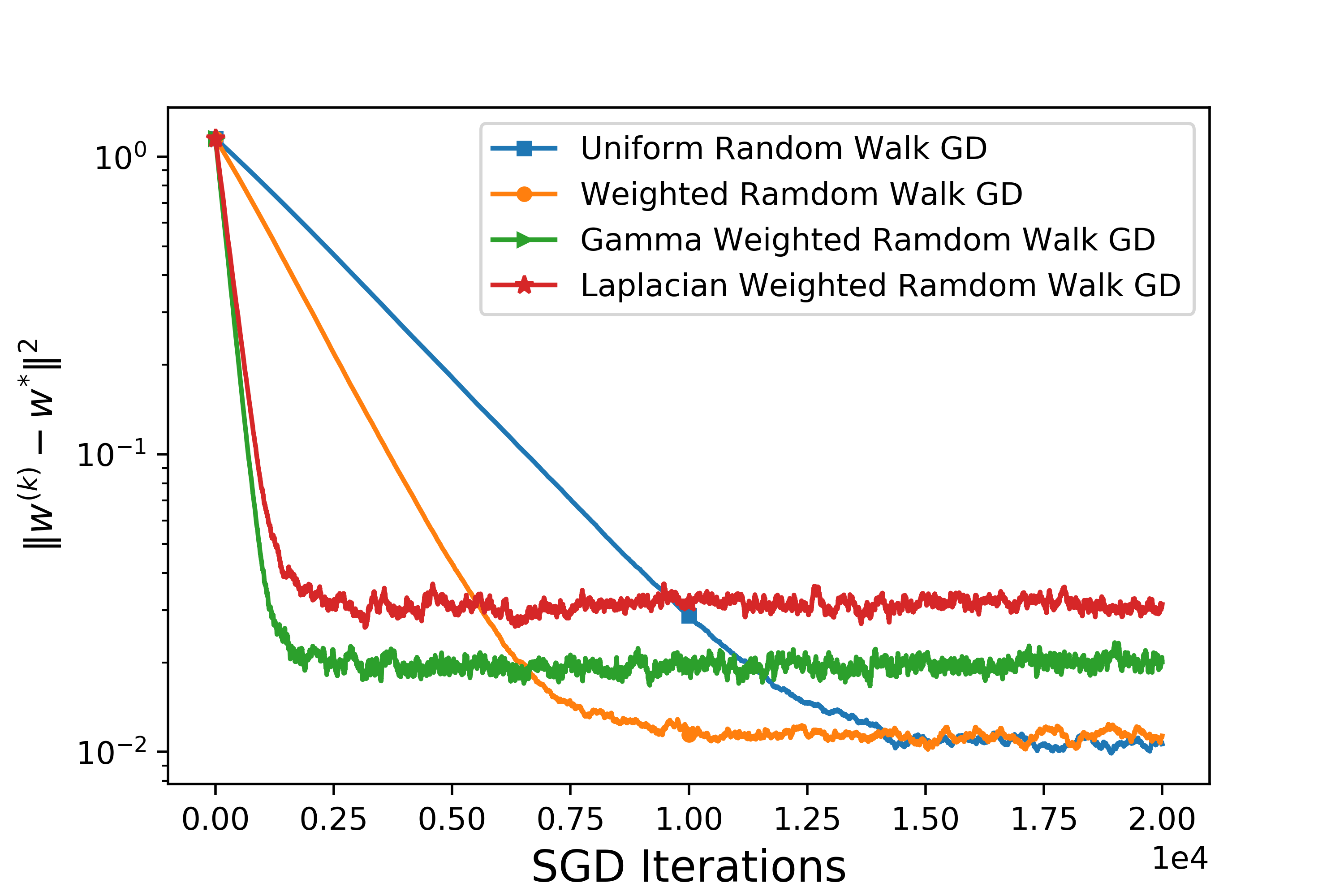
Figure 3: Error of the model estimated by the Uniform Random Walk SGD, $(3,\,0.03)$-LDP Gamma Weighted Random walk (Algorithm 3) and $(3,\,0)$-LDP Laplace Weighted Random walk on an Erdős-Rényi graph of $20$ nodes and probability of connectivity $p=0.3$.

VI Conclusion

In this paper, we study a decentralized learning problem where the data is distributed over the nodes of a graph. We propose decentralized learning algorithms based on random walk. To speed up the convergence, we propose a weighted random walk algorithm where the nodes get sampled depending on the importance of their data measured through the gradient-Lipschitz constant. A weighted random walk requires every node to share its gradient-Lipschitz constant with the neighbor nodes, which creates a privacy vulnarability. We propose a local differential privacy mechanism that we call Gamma mechanism to address the privacy concern, and give the tradeoff between the privacy parameters and the Gamma noise parameter. We also presented numerical results on the convergence of the proposed algorithms. As for future work, we think it is interesting to investigate different importance sampling measures for the weighted random walk.

Appendix A Proof of Theorem 1: Convergence Rate of Algorithm 1

First, we present preliminary results that will be used in the main proof later.

Lemma 4 (Lipschitzness).

If $f_{i}$ is a convex function on an open subset $\Omega\subseteq\mathbb{R}$, then for a closed bounded subset $\mathcal{W}\subset\Omega$, there exists a constant $D_{i}\geq 0$, such that, for any $w_{1},\,w_{2}\in\mathcal{W}$,

$$\left|f_{i}\left(w_{1}\right)-f_{i}\left(w_{2}\right)\right|\leq D_{i}\left\|w_{1}-w_{2}\right\|_{2}.$$

We define $D=\underset{i\in V}{\sup}D_{i}$. Therefore,

$$\left|f_{i}\left(w_{1}\right)-f_{i}\left(w_{2}\right)\right|\leq D\left\|w_{1}-w_{2}\right\|_{2}.$$

A proof for Lemma 4 can be found in [44].

Corollary 1 (Boundedness of the gradient).

If $f_{i}$ is a convex function on $\mathbb{R}$, then for a closed bounded subset $\mathcal{W}\subset\mathbb{R}$, $\left\|\nabla f_{i}(w)\right\|_{2}\leq D,\,\,\,\,\,\forall w\in\mathcal{W}.$

Proof.

Taking $v=w+\nabla f_{i}(w)$,

$$D\left\|\nabla f_{i}(w)\right\|_{2}=D\left\|v-w\right\|_{2}\overset{(a)}{\geq}|f_{i}(v)-f_{i}(w)|\overset{(b)}{\geq}\left\langle\nabla f_{i}\left(w\right),\nabla f_{i}\left(w\right)\right\rangle=\left\|\nabla f_{i}(w)\right\|_{2}^{2}.$$

(a) follows Lemma 4 and (b) follows from $f_{i}$ being convex.

∎

Next we give some results we need on the Markov chain. We remind the reader that $\pi$ is the stationary distribution, $P$ is the transition matrix and $P^{k}$ is the $k^{th}$ power of matrix P. We refer to $i^{th}$ row of a matrix $P$ by $P(i,:)$.

Lemma 5 (Convergence of Markov Chain [26]).

Under Assumption 2, we have

$$\underset{i}{\max}\left\|\pi-P^{k}\left(i,:\right)\right\|\leq C\lambda_{P}^{k}$$

for $k>K_{P}$, where $K_{P}$ is a constant that depends on $\lambda_{P}$ and $\lambda_{2}(P)$ and $C$ is a constant that depends on the Jordan canonical form of $P$.

Next, we start the proof for Theorem 1 following the same reasoning in [2] but with the inclusion of the gradient-Lipschitz assumption as in Assumption 1.

$$\left\|w^{(k+1)}-w^{*}\right\|_{2}^{2} =\left\|{\bf{\bf{\Pi}}_{\mathcal{W}}}\left(w^{(k)}-\gamma^{(k)}\nabla f_{i^{(k)}}\left(w^{(k)}\right)\right)-{\bf{\bf{\Pi}}_{\mathcal{W}}}\left(w^{*}\right)\right\|_{2}^{2}$$

$$\overset{\left(a\right)}{\leq}\left\|w^{(k)}-\gamma^{(k)}\nabla f_{i^{(k)}}\left(w^{(k)}\right)-w^{*}\right\|_{2}^{2}$$

$$=\left\|w^{(k)}-w^{*}\right\|_{2}^{2}-2\gamma^{(k)}\left\langle w^{(k)}-w^{*},\nabla f_{i^{(k)}}\left(w^{(k)}\right)\right\rangle$$

$$\,\,\,\,\,+\left(\gamma^{(k)}\right){}^{2}\left\|\nabla f_{i^{(k)}}\left(w^{(k)}\right)\right\|_{2}^{2}$$

$$=\left\|w^{(k)}-w^{*}\right\|_{2}^{2}-2\gamma^{(k)}\left\langle w^{(k)}-w^{*},\nabla f_{i^{(k)}}\left(w^{(k)}\right)\right\rangle$$

$$\,\,\,\,\,+\left(\gamma^{(k)}\right){}^{2}\left\|\nabla f_{i^{(k)}}\left(w^{(k)}\right)-\nabla f_{i^{(k)}}\left(w^{*}\right)+\nabla f_{i^{(k)}}\left(w^{*}\right)\right\|_{2}^{2}$$

$$\overset{\left(b\right)}{\leq}\left\|w^{(k)}-w^{*}\right\|_{2}^{2}-2\gamma^{(k)}\left\langle w^{(k)}-w^{*},\nabla f_{i^{(k)}}\left(w^{(k)}\right)\right\rangle$$

$$\,\,\,\,\,+2{(\gamma^{(k)})}^{2}\left\|\nabla f_{i^{(k)}}\left(w^{(k)}\right)-\nabla f_{i^{(k)}}\left(w^{*}\right)\right\|_{2}^{2}$$

$$\,\,\,\,\,+2{(\gamma^{(k)})}^{2}\left\|\nabla f_{i^{(k)}}\left(w^{*}\right)\right\|_{2}^{2}.$$ (14)

$\left(a\right)$ follows from $\mathcal{W}$ being a convex closed set, so one can apply nonexpansivity theorem [45, Fact E.9.0.0.5], $\left(b\right)$ follows from Jensen’s inequality applied to the squared norm.
Using Lemma 4 and the convexity of the functions $f_{i}$, we get

$$\left\|w^{(k+1)}-w^{*}\right\|_{2}^{2} \overset{\left(a\right)}{\leq}\left\|w^{(k)}-w^{*}\right\|_{2}^{2}-2\gamma^{(k)}\left\langle w^{(k)}-w^{*},\nabla f_{i^{(k)}}\left(w^{(k)}\right)\right\rangle$$

$$+2\left(\gamma^{(k)}\right){}^{2}L_{i^{(k)}}^{2}\left\|w^{(k)}-w^{*}\right\|_{2}^{2}+2\left(\gamma^{(k)}\right){}^{2}\left\|\nabla f_{i^{(k)}}\left(w^{*}\right)\right\|_{2}^{2}$$

$$\overset{\left(b\right)}{\leq}\left\|w^{(k)}-w^{*}\right\|_{2}^{2}-2\gamma^{(k)}\left\langle w^{(k)}-w^{*},\nabla f_{i^{(k)}}\left(w^{(k)}\right)\right\rangle$$

$$+2{(\gamma^{(k)})}^{2}\left(\sup L\right)^{2}\left\|w^{(k)}-w^{*}\right\|_{2}^{2}+2{(\gamma^{(k)})}^{2}\left\|\nabla f_{i}\left(w^{*}\right)\right\|_{2}^{2}.$$ (15)

$\left(a\right)$ follows from the Lipschitzness Lemma, $\left(b\right)$ follows by bounding by the $\sup L$.

For the next we use the convexity of $f_{i}$,

$$\left\|w^{(k+1)}-w^{*}\right\|^{2}_{2} \leq\left\|w^{(k)}-w^{*}\right\|_{2}^{2}-2\gamma^{(k)}\left(f_{i^{(k)}}\left(w^{(k)}\right)-f_{i^{(k)}}\left(w^{*}\right)\right)$$

$$+2{(\gamma^{(k)})}^{2}\left(\sup L\right)^{2}\left\|w^{(k)}-w^{*}\right\|_{2}^{2}$$

$$+2{(\gamma^{(k)})}^{2}\left\|\nabla f_{i^{(k)}}\left(w^{*}\right)\right\|_{2}^{2}.$$ (16)

By re-arranging (16), we come to

$$\gamma^{(k)}\left(f_{i^{(k)}}\left(w^{(k)}\right)-f_{i^{(k)}}\left(w^{*}\right)\right) \leq\frac{1}{2}\left(\left\|w^{(k)}-w^{*}\right\|_{2}^{2}-\left\|w^{(k+1)}-w^{*}\right\|_{2}^{2}\right)$$

$$\quad+{(\gamma^{(k)})}^{2}\left(\sup L\right)^{2}\left\|w^{(k)}-w^{*}\right\|_{2}^{2}$$

$$\quad+{(\gamma^{(k)})}^{2}\left\|\nabla f_{i^{(k)}}\left(w^{*}\right)\right\|_{2}^{2}.$$ (17)

Now summing (17) over $k$ and using Assumption 1 and the boundness of $\mathcal{W}$,

$$\sum_{k}\gamma^{(k)}\left(f_{i^{(k)}}\left(w^{(k)}\right)-f_{i^{(k)}}\left(w^{*}\right)\right) \leq\frac{1}{2}\left\|w^{(0)}-w^{*}\right\|_{2}^{2}+\left(\sup L\right)^{2}\sum_{k}(\gamma^{(k)})^{2}\left\|w^{(k)}-w^{*}\right\|_{2}^{2}$$

$$+\sum_{k}(\gamma^{(k)})^{2}\left\|\nabla f_{i^{(k)}}\left(w^{*}\right)\right\|_{2}^{2}<\infty.$$ (18)

We can see that the previous result shows the dependency on $\sup L$.

$$\gamma^{(k)}\mathbb{E}\left[f_{j^{(k)}}\left(w^{\left(k-T^{\left(k\right)}\right)}\right)-f_{j^{(k)}}\left(w^{(k)}\right)\right] \overset{(a)}{\leq}D\gamma^{(k)}\mathbb{E}\left\|w^{\left(k-T^{\left(k\right)}\right)}-w^{(k)}\right\|$$

$$\overset{(b)}{\leq}D\gamma^{(k)}\mathbb{E}\left(\sum_{n=k-T^{\left(k\right)}}^{k-1}\left\|w^{\left(n+1\right)}-w^{\left(n\right)}\right\|\right)$$

$$\overset{(c)}{\leq}D\gamma^{(k)}\sum_{n=k-T^{\left(k\right)}}^{k-1}\mathbb{E}\left(\left\|w^{\left(n+1\right)}-w^{\left(n\right)}\right\|\right)$$

$$\overset{(d)}{\leq}D^{2}\gamma^{(k)}\sum_{n=k-T^{\left(k\right)}}^{k-1}\gamma^{\left(n\right)}$$

$$\overset{(e)}{\leq}\frac{D^{2}}{2}\sum_{n=k-T^{\left(k\right)}}^{k-1}\left({(\gamma^{\left(n\right)})}^{2}+{(\gamma^{\left(k\right)})}^{2}\right)$$

$$\overset{}{\leq}\frac{D^{2}}{2}T^{\left(k\right)}{(\gamma^{\left(k\right)})}^{2}+\frac{D^{2}}{2}\sum_{n=k-T_{k}}^{k-1}{(\gamma^{\left(n\right)})}^{2}.$$

(a) follows from Lemma 4, (b) using triangle inequality, (c) using linearity of expectation, (d) follows Corollary 1 and (e) follows from the Cauchy–Schwarz inequality.

Now taking the summation over $k$:

$$\sum_{k}\gamma^{(k)}\mathbb{E}\left[f_{j^{(k)}}\left(w^{(k-T^{(k)})}\right)-f_{j^{(k)}}\left(w^{(k)}\right)\right]\leq\sum_{k}\frac{D^{2}}{2}T_{k}{(\gamma^{(k)})}^{2}+\frac{D^{2}}{2}\sum_{k}\sum_{n=k-T_{k}}^{k-1}{(\gamma^{(n)})}^{2}.$$ (19)

By simply using the assumption on the step size summability, the result is as follows:

$$\sum_{k=K}^{\infty}\sum_{n=k-T^{(k)}}^{k-1}\left(\gamma^{\left(n\right)}\right)^{2}\leq\sum_{k=K}^{\infty}T^{\left(k\right)}\left(\gamma^{(k)}\right)^{2}\leq\frac{2}{\ln\left(1/\lambda_{P}\right)}\sum_{k=K}^{\infty}\ln k.\left(\gamma^{(k)}\right)^{2}<\infty.$$ (20)

$$\mathbb{E}_{j^{(k)}}\left[f_{j^{(k)}}\left(w^{(k-T^{\left(k\right)})}\right)-f_{j^{(k)}}\left(w^{*}\right)|\,X_{0},\,X_{1},\,...,\,X_{k-T^{\left(k\right)}}\right]$$

$$\overset{}{=}\sum_{i=1}^{N}\left(f_{i}\left(w^{(k-T^{\left(k\right)})}\right)-f_{i}\left(w^{*}\right)\right)P\left(j^{(k)}=i\,|\,X_{0},\,X_{1},\,...,\,X_{k-T^{\left(k\right)}}\right)$$

$$\overset{(a)}{=}\sum_{i=1}^{N}\left(f_{i}\left(w^{(k-T^{\left(k\right)})}\right)-f_{i}\left(w^{*}\right)\right)P\left(j^{(k)}=i\,|\,X_{k-T^{\left(k\right)}}\right)$$

$$\overset{}{=}\sum_{i=1}^{N}\left(f_{i}\left(w^{(k-T^{\left(k\right)})}\right)-f_{i}\left(w^{*}\right)\right)P^{t_{k}}\left[X_{k-T^{\left(k\right)}}\,|\,j^{(k)}=i\right]$$

$$\overset{(b)}{\geq}\left(f\left(w^{(k-T^{\left(k\right)})}\right)-f\left(w^{*}\right)\right)-\frac{N}{2k}.$$

(a) using Markov property and (b) using Lemma 1 in [2].

Next, we get a bound on

$$\sum_{k}\gamma^{\left(k\right)}\mathbb{E}\left[f\left(w^{(k)}\right)-f\left(w^{(k-T^{\left(k\right)})}\right)\right].$$

$$\gamma^{(k)}\mathbb{E}\left[f\left(w^{\left(k-T_{k}\right)}\right)-f\left(w^{(k)}\right)\right] \overset{(a)}{\leq}ND\gamma^{(k)}\mathbb{E}\left\|w^{\left(k-T_{k}\right)}-w^{(k)}\right\|$$

$$\overset{(b)}{\leq}ND\gamma^{(k)}\mathbb{E}\left(\sum_{n=k-T_{k}}^{k-1}\left\|w^{\left(n+1\right)}-w^{\left(n\right)}\right\|\right)$$

$$\overset{(c)}{\leq}ND\gamma^{(k)}\sum_{n=k-T_{k}}^{k-1}\mathbb{E}\left(\left\|w^{\left(n+1\right)}-w^{\left(n\right)}\right\|\right)$$

$$\overset{(d)}{\leq}ND^{2}\gamma^{(k)}\sum_{n=k-T_{k}}^{k-1}\gamma^{\left(n\right)}$$

$$\overset{(e)}{\leq}\frac{ND^{2}}{2}\sum_{n=k-T_{k}}^{k-1}\left({(\gamma^{\left(n\right)})}^{2}+{(\gamma^{\left(k\right)})}^{2}\right)$$

$$\overset{}{\leq}\frac{ND^{2}}{2}T_{k}{(\gamma^{\left(k\right)})}^{2}+\frac{ND^{2}}{2}\sum_{n=k-T_{k}}^{k-1}{(\gamma^{\left(n\right)})}^{2}.$$

(a) follows from Lemma 4, (b) using triangle inequality, (c) using linearity of expectation, (d) follows Corollary 1 and (e) follows from the Cauchy–Schwarz inequality. The upper bound summability over $k$ follows from previous discussion in equation (20).

Combining with the results in (18) and (20) , we get

$$\sum_{k}\gamma^{(k)}\mathbb{E}\left[f\left(w^{(k-T_{k})}\right)-f\left(w^{*}\right)\right]\leq C_{1}\sigma^{2}+C_{2}\left(\sup L\right)^{2}+C_{3}\left(\frac{1}{\ln\left(1/\lambda_{P}\right)}\right).$$

Finally,

$$\mathbb{E}\left(f\left(\bar{w}^{(k)}\right)-f\left(w^{*}\right)\right)=O\left(\frac{\max\left(\sigma^{2},\,\left(\sup L\right)^{2},\,\frac{1}{\ln\left(1/\lambda_{P}\right)}\right)}{\left(\stackrel{{\scriptstyle[}}{{j}}=1]{k}{\sum}\gamma^{(k)}\right)}\right)=O\left(\frac{\max\left(\sigma^{2},\,\left(\sup L\right)^{2},\,\frac{1}{\ln\left(1/\lambda_{P}\right)}\right)}{k^{1-q}}\right).$$ (21)

Appendix B Proof of Theorem 2

To prove Theorem 2, we scale the local losses $f_{i}\left(w\right)$ in order to keep the same global loss under the new weighted sampling average is

$$f_{i,\,w}\left(w\right)=\frac{f_{i}\left(w\right)}{\frac{L_{i}}{\bar{L}}}=\frac{\bar{{L}}}{L_{i}}f_{i}\left(w\right).$$ (22)

For the next, we compute the gradient Lipschitz constant for the weighted loss function which is $L_{i,\,w}=\frac{L_{i}}{\frac{L_{i}}{\bar{L}}}=\bar{{L}}.$

Here, we get $\sup L_{w}:=\underset{i}{\max}L_{i,\,w}=\bar{{L}}.$ After we compute the new residual quantity that also contributes to the rate of convergence:

$$\sum_{i=1}^{N}\frac{L_{i}}{N\bar{{L}}}\left\|\nabla f_{i,\,w}\left(w^{*}\right)\right\|_{2}^{2} =\sum_{i=1}^{N}\frac{L_{i}}{N\bar{{L}}}\left(\frac{\bar{L}}{L_{i}}\right)^{2}\left\|\nabla f_{i}\left(w^{*}\right)\right\|_{2}^{2}$$

$$=\sum_{i=1}^{N}\frac{1}{N}\left(\frac{\bar{L}}{L_{i}}\right)\left\|\nabla f_{i}\left(w^{*}\right)\right\|_{2}^{2}$$

$$\leq\frac{\bar{L}}{\inf L}\left(\sum_{i=1}^{N}\frac{1}{N}\left\|\nabla f_{i}\left(w^{*}\right)\right\|_{2}^{2}\right).$$

Appendix C Private Random Walk SGD

Using the Gamma noise on the gradient-Lipschitz constants in the weighted random walk ends up giving unbiased gradient estimate at the stationary regime:

$$\mathbb{E}_{\mathcal{R}}\mathbb{E}_{\pi_{w,\,\mathcal{R}}}\left[\hat{\nabla}f_{i}\,|\,\mathcal{R}\left(L_{j}\right),\,j=1,\,...,\,N\right] =\nabla f.$$

Proof.

$$\mathbb{E}_{\mathcal{R}}\mathbb{E}_{\pi_{w,\,\mathcal{R}}}\left[\hat{\nabla}f_{i}\,|\,\mathcal{R}\left(L_{j}\right),\,j=1,\,...,\,N\right] =\mathbb{E}_{\mathcal{R}}\mathbb{E}_{\pi_{w,\,\mathcal{R}}}\left[\frac{\bar{L}}{L_{i}}\nabla f_{i}|\,\mathcal{R}\left(L_{j}\right),\,j=1,\,...,\,N\right]$$

$$=\sum_{i}\mathbb{E}_{\mathcal{R}}\left[\frac{\mathcal{R}\left(L_{i}\right)}{\sum_{j}\mathcal{R}\left(L_{j}\right)}\frac{\sum_{j}L_{j}}{NL_{i}}\nabla f_{i}\right]$$

$$=\mathbb{E}_{i}\left[\nabla f_{i}\right]=\nabla f.$$

∎

Appendix D Proof of Lemma 3

We will use the following property for $(\epsilon,\,\delta)$ differentially mechanism.

Lemma 6.

[25]

A mechanism is $(\epsilon,\delta)$-differentially private if, for any $L,\,L^{\prime}$, and $Z$ a random variable with the same distribution as $\mathcal{R}(L)$, we have

$$P(\log\frac{P_{\mathcal{R}\left(L\right)}\left(z\right)}{P_{\mathcal{R}\left(L^{\prime}\right)}\left(z\right)}\geq\epsilon)\leq\delta.$$

In our case, $Z\sim Gamma(L,\,\theta)$.

Now, for the proof of Lemma 3, taking $L,\,L^{\prime}$ and a received output $z\in\mathbb{R}$, we have

$$\frac{P_{\mathcal{R}\left(L\right)}\left(z\right)}{P_{\mathcal{R}\left(L^{\prime}\right)}\left(z\right)}=\frac{\frac{1}{\Gamma\left(L/\theta\right)\theta^{\frac{L}{\theta}}}z^{\frac{L}{\theta}-1}e^{\frac{z}{\theta}}}{\frac{1}{\Gamma\left(L^{\prime}/\theta\right)\theta^{\frac{L^{\prime}}{\theta}}}z^{\frac{L^{\prime}}{\theta}-1}e^{\frac{z}{\theta}}}=\frac{\Gamma\left(L^{\prime}/\theta\right)}{\Gamma\left(L/\theta\right)}\theta^{\frac{L^{\prime}-L}{\theta}}z^{\frac{L-L^{\prime}}{\theta}}.$$

Then, taking a random variable $Z$ on $z$, where $Z\sim Gamma(L,\,\theta)$:

$$\left(\frac{Z}{\theta}\right)^{\frac{L-L^{\prime}}{\theta}}\sim{Generalized\,Gamma}\left(p=\frac{\theta}{L-L^{\prime}},\,d=\frac{L}{L-L^{\prime}},\,1\right),$$

$$\quad\text{when}\,L>L^{\prime}.$$

As a reminder, the probability density function of the Generalized Gamma function on a random variable $Y$ is

$$p_{GG,\,Y}(y)=\frac{p/a^{d}}{\Gamma\left(d/p\right)}y^{d-1}e^{-\left(y/a\right)^{p}}\qquad y>0,\quad a,d,p>0.$$

When $L>L^{\prime}$, we have

$$P\left(\frac{\Gamma\left(L^{\prime}/\theta\right)}{\Gamma\left(L/\theta\right)}\theta^{\frac{L^{\prime}-L}{\theta}}Z^{\frac{L-L^{\prime}}{\theta}}\geq e^{\epsilon}\right) =P\left(\left(\frac{Z}{\theta}\right)^{\frac{L-L^{\prime}}{\theta}}\geq e^{\epsilon}\frac{\Gamma\left(L/\theta\right)}{\Gamma\left(L^{\prime}/\theta\right)}\right)$$

$$=1-P\left(\left(\frac{Z}{\theta}\right)^{\frac{L-L^{\prime}}{\theta}}\leq e^{\epsilon}\frac{\Gamma\left(L/\theta\right)}{\Gamma\left(L^{\prime}/\theta\right)}\right)$$

$$=1-\frac{IG\left(\frac{L}{\theta},\left(e^{\epsilon}\frac{\Gamma\left(L/\theta\right)}{\Gamma\left(L^{\prime}/\theta\right)}\right)^{\frac{\theta}{L^{\prime}-L}}\right)}{\Gamma\left(L/\theta\right)}$$

$$\leq\delta,$$

where $IG$ is the lower incomplete gamma function.

When $L<L^{\prime}$, we have

$$P\left(\frac{\Gamma\left(L^{\prime}/\theta\right)}{\Gamma\left(L/\theta\right)}\theta^{\frac{L^{\prime}-L}{\theta}}Z^{\frac{L-L^{\prime}}{\theta}}\geq e^{\epsilon}\right) =P\left(\left(\frac{Z}{\theta}\right)^{\frac{L^{\prime}-L}{\theta}}\leq\frac{\Gamma\left(L^{\prime}/\theta\right)}{\Gamma\left(L/\theta\right)e^{\epsilon}}\right)$$

$$=\frac{IG\left(\frac{L}{\theta},\left(\frac{\Gamma\left(L^{\prime}/\theta\right)}{\Gamma\left(L/\theta\right)e^{\epsilon}}\right)^{\frac{\theta}{L^{\prime}-L}}\right)}{\Gamma\left(L/\theta\right)}$$

$$\leq\delta.$$

References

- [1] S. S. Ram, A. Nedic, and V. V. Veeravalli, “Asynchronous gossip algorithms for stochastic optimization,” 2009 International Conference on Game Theory for Networks, pp. 80–81, 2009.
- [2] T. Sun, Y. Sun, and W. Yin, “On markov chain gradient descent,” in NeurIPS, 2018.
- [3] D. Needell, R. Ward, and N. Srebro, “Stochastic Gradient Descent, Weighted Sampling, and the Randomized Kaczmarz algorithm,” in Advances in Neural Information Processing Systems 27, Z. Ghahramani, M. Welling, C. Cortes, N. D. Lawrence, and K. Q. Weinberger, Eds. Curran Associates, Inc., 2014, pp. 1017–1025.
- [4] B. Johansson, M. Rabi, and M. Johansson, “A simple peer-to-peer algorithm for distributed optimization in sensor networks,” 2007 46th IEEE Conference on Decision and Control, pp. 4705–4710, 2007.
- [5] ——, “A randomized incremental subgradient method for distributed optimization in networked systems,” SIAM J. Optim., vol. 20, pp. 1157–1170, 2009.
- [6] A. Nedic and A. Ozdaglar, “Distributed subgradient methods for multi-agent optimization,” IEEE Transactions on Automatic Control, vol. 54, pp. 48–61, 2009.
- [7] H. Wai, N. Freris, A. Nedic, and A. Scaglione, “Sucag: Stochastic unbiased curvature-aided gradient method for distributed optimization,” 2018 IEEE Conference on Decision and Control (CDC), pp. 1751–1756, 2018.
- [8] H. Wai, W. Shi, A. Nedic, and A. Scaglione, “Curvature-aided incremental aggregated gradient method,” 2017 55th Annual Allerton Conference on Communication, Control, and Computing (Allerton), pp. 526–532, 2017.
- [9] X. Mao, K. Yuan, Y. Hu, Y. Gu, A. H. Sayed, and W. Yin, “Walkman: A communication-efficient random-walk algorithm for decentralized optimization,” IEEE Transactions on Signal Processing, vol. 68, pp. 2513–2528, 2020.
- [10] S. P. Boyd, A. Ghosh, B. Prabhakar, and D. Shah, “Randomized gossip algorithms,” IEEE Transactions on Information Theory, vol. 52, pp. 2508–2530, 2006.
- [11] A. Koloskova, S. Stich, and M. Jaggi, “Decentralized stochastic optimization and gossip algorithms with compressed communication,” ArXiv, vol. abs/1902.00340, 2019.
- [12] T. Aysal, M. E. Yildiz, A. Sarwate, and A. Scaglione, “Broadcast gossip algorithms for consensus,” IEEE Transactions on Signal Processing, vol. 57, pp. 2748–2761, 2009.
- [13] J. C. Duchi, A. Agarwal, and M. Wainwright, “Dual averaging for distributed optimization: Convergence analysis and network scaling,” IEEE Transactions on Automatic Control, vol. 57, pp. 592–606, 2012.
- [14] J. C. Duchi, M. I. Jordan, and M. J. Wainwright, “Local privacy and statistical minimax rates,” in 2013 IEEE 54th Annual Symposium on Foundations of Computer Science. IEEE, 2013, pp. 429–438.
- [15] P. Kairouz, S. Oh, and P. Viswanath, “Extremal mechanisms for local differential privacy,” in Advances in neural information processing systems, 2014, pp. 2879–2887.
- [16] X. Wu, A. Kumar, K. Chaudhuri, S. Jha, and J. F. Naughton, “Differentially private stochastic gradient descent for in-rdbms analytics,” ArXiv, vol. abs/1606.04722, 2016.
- [17] R. Bassily, A. D. Smith, and A. Thakurta, “Private empirical risk minimization: Efficient algorithms and tight error bounds,” 2014 IEEE 55th Annual Symposium on Foundations of Computer Science, pp. 464–473, 2014.
- [18] V. Gandikota, R. K. Maity, and A. Mazumdar, “vqsgd: Vector quantized stochastic gradient descent,” ArXiv, vol. abs/1911.07971, 2019.
- [19] S. Xiong, A. D. Sarwate, and N. B. Mandayam, “Randomized requantization with local differential privacy,” 2016 IEEE International Conference on Acoustics, Speech and Signal Processing (ICASSP), pp. 2189–2193, 2016.
- [20] W.-N. Chen, P. Kairouz, and A. Özgür, “Breaking the communication-privacy-accuracy trilemma,” ArXiv, vol. abs/2007.11707, 2020.
- [21] P. Zhao and T. Zhang, “Stochastic optimization with importance sampling,” ArXiv, vol. abs/1401.2753, 2014.
- [22] G. Ayache and S. E. Rouayheb, “Random walk gradient descent for decentralized learning on graphs,” 2019 IEEE International Parallel and Distributed Processing Symposium Workshops (IPDPSW), pp. 926–931, 2019.
- [23] D. P. Bertsekas, “Nonlinear programming,” Journal of the Operational Research Society, vol. 48, p. 334, 1995.
- [24] C. Dwork and A. Roth, “The algorithmic foundations of differential privacy,” Foundations and Trends in Theoretical Computer Science, vol. 9, pp. 211–407, 2014.
- [25] M. Bun and T. Steinke, “Concentrated differential privacy: Simplifications, extensions, and lower bounds,” ArXiv, vol. abs/1605.02065, 2016.
- [26] D. A. Levin, Y. Peres, and E. L. Wilmer, Markov chains and mixing times. American Mathematical Society, 2006.
- [27] H. E. Robbins, “A stochastic approximation method,” Annals of Mathematical Statistics, vol. 22, pp. 400–407, 2007.
- [28] L. Bottou, “Large-scale machine learning with stochastic gradient descent,” in COMPSTAT, 2010.
- [29] F. R. Bach and E. Moulines, “Non-asymptotic analysis of stochastic approximation algorithms for machine learning,” in NIPS, 2011.
- [30] C.-H. Lee, X. Xu, and D. Y. Eun, “Beyond random walk and metropolis-hastings samplers: why you should not backtrack for unbiased graph sampling,” in SIGMETRICS, 2012.
- [31] B. Chen, Y. Xu, and A. Shrivastava, “Fast and accurate stochastic gradient estimation,” in NeurIPS, 2019.
- [32] Z. Borsos, S. Curi, K. Y. Levy, and A. Krause, “Online variance reduction with mixtures,” in ICML, 2019.
- [33] G. Alain, A. Lamb, C. Sankar, A. C. Courville, and Y. Bengio, “Variance reduction in sgd by distributed importance sampling,” ArXiv, vol. abs/1511.06481, 2015.
- [34] G. Bouchard, T. Trouillon, J. Perez, and A. Gaidon, “Online learning to sample,” 2015.
- [35] L. Bottou and O. Bousquet, “The tradeoffs of large scale learning,” in NIPS, 2007.
- [36] F. R. Bach and E. Moulines, “Non-strongly-convex smooth stochastic approximation with convergence rate o(1/n),” in NIPS, 2013.
- [37] J. C. Duchi, A. Agarwal, M. Johansson, and M. I. Jordan, “Ergodic mirror descent,” 2011 49th Annual Allerton Conference on Communication, Control, and Computing (Allerton), pp. 701–706, 2011.
- [38] W. Shi, Q. Ling, G. Wu, and W. Yin, “Extra: An exact first-order algorithm for decentralized consensus optimization,” SIAM J. Optim., vol. 25, pp. 944–966, 2015.
- [39] A. I. Chen, “Fast distributed first-order methods,” 2012.
- [40] D. Jakovetić, J. Xavier, and J. M. F. Moura, “Fast distributed gradient methods,” IEEE Transactions on Automatic Control, vol. 59, pp. 1131–1146, 2014.
- [41] A. Koloskova, N. Loizou, S. Boreiri, M. Jaggi, and S. Stich, “A unified theory of decentralized sgd with changing topology and local updates,” ArXiv, vol. abs/2003.10422, 2020.
- [42] A. Papoulis and S. Pillai, “Probability, random variables, and stochastic processes, fourth edition,” 2002.
- [43] A. Kim, “Beta distribution: Intuition, examples, and derivation,” January 2020, https://towardsdatascience.com/beta-distribution-intuition-examples-and-derivation-cf00f4db57af, [Online; posted 08-January-2020].
- [44] “Every Convex Function is Locally Lipschitz,” The American Mathematical Monthly, vol. 79, no. 10, pp. 1121–1124, 1972. [Online]. Available: http://www.jstor.org/stable/2317434
- [45] J. C. Dattorro, “Convex optimization and euclidean distance geometry,” 2004.

References

- [1] S. S. Ram, A. Nedic, and V. V. Veeravalli, “Asynchronous gossip algorithms for stochastic optimization,” 2009 International Conference on Game Theory for Networks, pp. 80–81, 2009.
- [2] T. Sun, Y. Sun, and W. Yin, “On markov chain gradient descent,” in NeurIPS, 2018.
- [3] D. Needell, R. Ward, and N. Srebro, “Stochastic Gradient Descent, Weighted Sampling, and the Randomized Kaczmarz algorithm,” in Advances in Neural Information Processing Systems 27, Z. Ghahramani, M. Welling, C. Cortes, N. D. Lawrence, and K. Q. Weinberger, Eds. Curran Associates, Inc., 2014, pp. 1017–1025.
- [4] B. Johansson, M. Rabi, and M. Johansson, “A simple peer-to-peer algorithm for distributed optimization in sensor networks,” 2007 46th IEEE Conference on Decision and Control, pp. 4705–4710, 2007.
- [5] ——, “A randomized incremental subgradient method for distributed optimization in networked systems,” SIAM J. Optim., vol. 20, pp. 1157–1170, 2009.
- [6] A. Nedic and A. Ozdaglar, “Distributed subgradient methods for multi-agent optimization,” IEEE Transactions on Automatic Control, vol. 54, pp. 48–61, 2009.
- [7] H. Wai, N. Freris, A. Nedic, and A. Scaglione, “Sucag: Stochastic unbiased curvature-aided gradient method for distributed optimization,” 2018 IEEE Conference on Decision and Control (CDC), pp. 1751–1756, 2018.
- [8] H. Wai, W. Shi, A. Nedic, and A. Scaglione, “Curvature-aided incremental aggregated gradient method,” 2017 55th Annual Allerton Conference on Communication, Control, and Computing (Allerton), pp. 526–532, 2017.
- [9] X. Mao, K. Yuan, Y. Hu, Y. Gu, A. H. Sayed, and W. Yin, “Walkman: A communication-efficient random-walk algorithm for decentralized optimization,” IEEE Transactions on Signal Processing, vol. 68, pp. 2513–2528, 2020.
- [10] S. P. Boyd, A. Ghosh, B. Prabhakar, and D. Shah, “Randomized gossip algorithms,” IEEE Transactions on Information Theory, vol. 52, pp. 2508–2530, 2006.
- [11] A. Koloskova, S. Stich, and M. Jaggi, “Decentralized stochastic optimization and gossip algorithms with compressed communication,” ArXiv, vol. abs/1902.00340, 2019.
- [12] T. Aysal, M. E. Yildiz, A. Sarwate, and A. Scaglione, “Broadcast gossip algorithms for consensus,” IEEE Transactions on Signal Processing, vol. 57, pp. 2748–2761, 2009.
- [13] J. C. Duchi, A. Agarwal, and M. Wainwright, “Dual averaging for distributed optimization: Convergence analysis and network scaling,” IEEE Transactions on Automatic Control, vol. 57, pp. 592–606, 2012.
- [14] J. C. Duchi, M. I. Jordan, and M. J. Wainwright, “Local privacy and statistical minimax rates,” in 2013 IEEE 54th Annual Symposium on Foundations of Computer Science. IEEE, 2013, pp. 429–438.
- [15] P. Kairouz, S. Oh, and P. Viswanath, “Extremal mechanisms for local differential privacy,” in Advances in neural information processing systems, 2014, pp. 2879–2887.
- [16] X. Wu, A. Kumar, K. Chaudhuri, S. Jha, and J. F. Naughton, “Differentially private stochastic gradient descent for in-rdbms analytics,” ArXiv, vol. abs/1606.04722, 2016.
- [17] R. Bassily, A. D. Smith, and A. Thakurta, “Private empirical risk minimization: Efficient algorithms and tight error bounds,” 2014 IEEE 55th Annual Symposium on Foundations of Computer Science, pp. 464–473, 2014.
- [18] V. Gandikota, R. K. Maity, and A. Mazumdar, “vqsgd: Vector quantized stochastic gradient descent,” ArXiv, vol. abs/1911.07971, 2019.
- [19] S. Xiong, A. D. Sarwate, and N. B. Mandayam, “Randomized requantization with local differential privacy,” 2016 IEEE International Conference on Acoustics, Speech and Signal Processing (ICASSP), pp. 2189–2193, 2016.
- [20] W.-N. Chen, P. Kairouz, and A. Özgür, “Breaking the communication-privacy-accuracy trilemma,” ArXiv, vol. abs/2007.11707, 2020.
- [21] P. Zhao and T. Zhang, “Stochastic optimization with importance sampling,” ArXiv, vol. abs/1401.2753, 2014.
- [22] G. Ayache and S. E. Rouayheb, “Random walk gradient descent for decentralized learning on graphs,” 2019 IEEE International Parallel and Distributed Processing Symposium Workshops (IPDPSW), pp. 926–931, 2019.
- [23] D. P. Bertsekas, “Nonlinear programming,” Journal of the Operational Research Society, vol. 48, p. 334, 1995.
- [24] C. Dwork and A. Roth, “The algorithmic foundations of differential privacy,” Foundations and Trends in Theoretical Computer Science, vol. 9, pp. 211–407, 2014.
- [25] M. Bun and T. Steinke, “Concentrated differential privacy: Simplifications, extensions, and lower bounds,” ArXiv, vol. abs/1605.02065, 2016.
- [26] D. A. Levin, Y. Peres, and E. L. Wilmer, Markov chains and mixing times. American Mathematical Society, 2006.
- [27] H. E. Robbins, “A stochastic approximation method,” Annals of Mathematical Statistics, vol. 22, pp. 400–407, 2007.
- [28] L. Bottou, “Large-scale machine learning with stochastic gradient descent,” in COMPSTAT, 2010.
- [29] F. R. Bach and E. Moulines, “Non-asymptotic analysis of stochastic approximation algorithms for machine learning,” in NIPS, 2011.
- [30] C.-H. Lee, X. Xu, and D. Y. Eun, “Beyond random walk and metropolis-hastings samplers: why you should not backtrack for unbiased graph sampling,” in SIGMETRICS, 2012.
- [31] B. Chen, Y. Xu, and A. Shrivastava, “Fast and accurate stochastic gradient estimation,” in NeurIPS, 2019.
- [32] Z. Borsos, S. Curi, K. Y. Levy, and A. Krause, “Online variance reduction with mixtures,” in ICML, 2019.
- [33] G. Alain, A. Lamb, C. Sankar, A. C. Courville, and Y. Bengio, “Variance reduction in sgd by distributed importance sampling,” ArXiv, vol. abs/1511.06481, 2015.
- [34] G. Bouchard, T. Trouillon, J. Perez, and A. Gaidon, “Online learning to sample,” 2015.
- [35] L. Bottou and O. Bousquet, “The tradeoffs of large scale learning,” in NIPS, 2007.
- [36] F. R. Bach and E. Moulines, “Non-strongly-convex smooth stochastic approximation with convergence rate o(1/n),” in NIPS, 2013.
- [37] J. C. Duchi, A. Agarwal, M. Johansson, and M. I. Jordan, “Ergodic mirror descent,” 2011 49th Annual Allerton Conference on Communication, Control, and Computing (Allerton), pp. 701–706, 2011.
- [38] W. Shi, Q. Ling, G. Wu, and W. Yin, “Extra: An exact first-order algorithm for decentralized consensus optimization,” SIAM J. Optim., vol. 25, pp. 944–966, 2015.
- [39] A. I. Chen, “Fast distributed first-order methods,” 2012.
- [40] D. Jakovetić, J. Xavier, and J. M. F. Moura, “Fast distributed gradient methods,” IEEE Transactions on Automatic Control, vol. 59, pp. 1131–1146, 2014.
- [41] A. Koloskova, N. Loizou, S. Boreiri, M. Jaggi, and S. Stich, “A unified theory of decentralized sgd with changing topology and local updates,” ArXiv, vol. abs/2003.10422, 2020.
- [42] A. Papoulis and S. Pillai, “Probability, random variables, and stochastic processes, fourth edition,” 2002.
- [43] A. Kim, “Beta distribution: Intuition, examples, and derivation,” January 2020, https://towardsdatascience.com/beta-distribution-intuition-examples-and-derivation-cf00f4db57af, [Online; posted 08-January-2020].
- [44] “Every Convex Function is Locally Lipschitz,” The American Mathematical Monthly, vol. 79, no. 10, pp. 1121–1124, 1972. [Online]. Available: http://www.jstor.org/stable/2317434
- [45] J. C. Dattorro, “Convex optimization and euclidean distance geometry,” 2004.