Eliciting Information from Sensitive Survey Questions

Abstract

This paper considers how to elicit information from sensitive survey questions. First we thoroughly evaluate list experiments (LE), a leading method in the experimental literature on sensitive questions. Our empirical results demonstrate that the assumptions required to identify sensitive information in LE are violated for the majority of surveys. Next we propose a novel survey method, called Multiple Response Technique (MRT), for eliciting information from sensitive questions. We require all of the respondents to answer three questions related to the sensitive information. This technique recovers sensitive information at a disaggregated level while still allowing arbitrary misreporting in survey responses. An application of the MRT provides novel empirical evidence on sexual orientation and Lesbian, Gay, Bisexual, and Transgender (LGBT)-related sentiment.

Keywords: list experiments, measurement error, sensitive information, sensitive questions, survey data, LGBT

JEL: D8, C1

1 Introduction

Surveys designed to address a wide range of social and economic issues—such as racial prejudice, drug use, illegal immigration, and fraud—often elicit information on private, illegal, or socially undesirable behaviors. However, respondents tend to misreport their views on sensitive topics, and that misreported information often leads to biased estimates of the behaviors, their determinants, and their causal effects.

Estimating sensitive information from potentially misreported data has important implications for social and economic policy decisions. Therefore, methods that produce unbiased estimates are prominent. The method of list experiments (LE), also known as the “item count technique” and “unmatched count technique”, is one of the most popular methods used to reduce response bias in surveys. It was proposed in Raghavarao and Federer (1979) to enhance respondents’ willingness to answer truthfully by anonymizing the survey. In LE, a sample of respondents are randomly assigned to a control and a treatment group. The control group receives a set of nonsensitive questions; the treatment group receives the same set of questions plus one sensitive question. The respondents in both groups only indicate the number of applicable items. Coffman et al. (2017) further develop LE by modifying the survey design: the control group is required to answer the sensitive question directly, in addition to indicating the number of applicable nonsensitive items.

LE has been widely used in the past three decades in multiple disciplines, including political science, sociology, psychology, and statistics, and it has been applied increasingly in economics recently. When searched the keywords “list experiments”, “item count technique”, and “unmatched count technique”, we found 20 economics articles using the method after 2010, with 13 of them published after 2016. The American Economic Review and Quarterly Journal of Economics had no publications using LE before 2016, but published six articles using it during 2016-2019.

Despite its wide applications, LE has never been assessed systematically for its validity. Thus the reliability of empirical results based on the LE method is unclear. In this paper, we develop a method to evaluate LE and then show that the assumptions required to identify sensitive information in LE are violated for the majority of its empirical applications. In addition to a high likelihood of failure, LE, and other existing methods of eliciting sensitive information only provide a measure of sensitive information at the aggregate level. This limits the use of the aggregated measure as an outcome variable (Bertrand and Duflo (2017)). To address these issues, we propose a novel method, multiple response technique (MRT), to elicit sensitive information from survey questions. Our method is applicable to surveys with measurement error due to misreporting, regardless of the presence of sensitive information.

We begin by providing a rigorous framework for LE. First, we generalize LE by relaxing a ubiquitous assumption that respondents will answer survey questions truthfully. In our generalized model, respondents in the control and treatment groups may misreport, and may do so in different ways. Truthful response is nested as a special case of the generalized model where the misreporting probability equals zero. We show that in the generalized model, if respondents are randomly assigned into two groups and the sensitive item does not alter the preferences of respondents in the treatment group, then restrictions on the observed responses imposed by LE can be summarized as a set of moment conditions. The model’s parameters, including the proportion of respondents with sensitive information and misreporting probabilities, can be estimated from the moment conditions through the generalized method of moments (GMM) if there are at least three nonsensitive questions. We find that using mean difference (difference between means of applicable items in the two groups), the commonly used approach to estimating the proportion of respondents with sensitive information is generally biased in the presence of misreporting. The magnitude of the bias depends on the true parameters of the model, the number of nonsensitive questions, and misreporting probabilities.

Based on the moment conditions just described, we develop a procedure for testing the validity of the basic assumptions of LE. We apply our test to five recently published articles where the results depend partially on LE. For the majority of the empirical applications, the fundamental assumptions are violated. Thus, estimates based on LE through different methods–including mean difference, ordinary least squares (OLS), nonlinear least squares (NLS), and maximum likelihood estimation (MLE)–would be biased and the implications of those estimates, together with their determinants and causal effects, are problematic. The problems with LE could be due to the significance of misreporting, the non-randomness of group assignment, or the impacts of the sensitive item on respondents’ preference. However, in the literature it is unclear how we can make adjustments to LE to obtain unbiased estimates once its fundamental assumptions fail.

Therefore, we propose a novel method of eliciting information from sensitive survey questions. Respondents receive three or more survey questions related to the sensitive information. Random assignment to groups is not required. We treat the sensitive information as respondents’ unobserved heterogeneity and recover it from their responses to multiple survey questions. Our method’s validity is based on two assumptions: (1) after we control the set of observed (e.g., demographic) variables and the sensitive information, the respondent’s responses to three survey questions will be independent; and (2) respondents with or without sensitive information will answer some survey questions differently. Given a sample of the survey responses and respondents’ characteristics, we then propose two versions of estimation suitable for the different data patterns. When the covariates are discrete, it is convenient to estimate model primitives using a closed-form and nonparametric procedure. One prominent property of the nonparametric approach is that it is global and involves no numerical optimizations. When the covariates are continuous, we apply maximum likelihood estimation (MLE) to estimate the dependence of sensitive behaviors on the covariates. The resulting estimates allow us to predict the likelihood of sensitive behaviors for a given value of the covariates. Monte Carlo simulations show good performance of both estimating procedures with a modest sample size.

Our proposed method has several important advantages over LE and other approaches to eliciting sensitive information. First, we can recover sensitive information at a disaggregated level. For example, in a study of respondents’ attitude toward same-sex marriage, we are able to recover the proportions of supporters for both LGBT and non-LGBT populations, while the existing methods only provide an overall proportion. Second, our proposed method allows misreporting in an arbitrary form, and the measurement error due to that misreporting can be recovered. When a sample of respondents are asked about their sexuality in a survey question, we can estimate the measurement error of their responses. And last but not least, the effects of group assignment on survey results are ruled out because respondents are not grouped.

Using our proposed method we estimate sexual orientation and LGBT-related sentiment. The data were analyzed in Coffman et al. (2017), where the main objective was to illustrate the substantially underestimated size of the LGBT-population and the magnitude of anti-gay sentiment. We apply our proposed technique to this data and our analysis leads to several novel findings that are obscured with LE and other existing survey methods.

Ours are the first set of quantitative results in the literature on respondents’ misreporting behavior when indicating their sexual orientation, and on how the dependence of misreporting behavior depends on demographics. A substantial portion (about 28.8%) of non-heterosexual respondents report themselves to be heterosexual, while heterosexual respondents report truthfully. Male, Black, Christian, and Republican respondents report a much lower proportion of non-heterosexuality than their counterpart groups. For example, 47.3% of non-heterosexual Republicans claim themselves to be heterosexual while the comparable percentage is only 25.6% for Democrats. These results are obtained without any ex ante information on respondents’ sexual orientation.

Respondents with negative sentiments to the LGBT population are significantly divided. Black, Christian, and Republican respondents are substantially more negative toward the LGBT population than their counterparts: for example, 22% of Christian respondents have negative sentiments, while the proportion is only 3.2% for non-religious respondents. We also find significant divergence on how respondents with negative sentiments toward the LGBT population respond to the three sentiment-related questions. “Happy with LGB manager” is accepted by only 2% of the respondents, while 17.8% of them support same-sex marriage and 58.5% of them “believe it is illegal to discriminate against LGBT people”. These estimates exhibit sharp divides among demographic groups, and the attitude toward same-sex marriage is the most diverse for the three questions: the proportion of white respondents who support same-sex marriage is five times that of Black respondents; for nonreligious respondents it is three times that of Christian; and for Democrats is five times that of Republicans.

This paper contributes to a broader literature on surveys and related empirical studies. First of all, we develop a rigorous procedure to check whether LE is applicable to the survey data. There are now two strands of literature on the applications of LE. The first focuses on estimating the proportion of sensitive behavior, its determinants and consequences. The applications cover a wide range of topics in economics, including anti-authoritarian movements (Cantoni et al. (2019)); criminal behavior (Kuha and Jackson (2014)); the effects of labor exclusion on responsibilities (Ronconi and SJ (2015)); election (Neggers (2018) and Barrera et al. (2020)); evaluation of anti-poverty programs (Haushofer and Shapiro (2016) and Muralidharan et al. (2016)); impacts of media censorship (Chen and Yang (2019)); influence of exporting democracy (Humphreys et al. (2019)); microfinance (Karlan and Zinman (2012) and Karlan et al. (2016)); relationship between financial conditions and performance of firms (Bilir et al. (2019)); and sexual health (Chong et al. (2013) and Treibich and Lépine (2019)). The second strand relies on the modified LE in Coffman et al. (2017) to justify the reliability of survey data. If the proportion of affirmative answers to the sensitive question in the control group is the same as the mean difference, then misreporting does not exist or is negligible, e.g., see Cantoni et al. (2019) and Chen and Yang (2019) for applications. All of these applications assume that the basic assumptions of LE hold, without checking their validity. To the best of our knowledge, we are the first to empirically evaluate the validity of the assumptions in the LE approach. Our negative findings suggest that researchers should be cautious when applying LE and interpreting empirical results based on LE.

Second, although our proposed technique is motivated by the potential failure of LE, the applicability of our MRT technique is more general. Our technique has its flexibility to address various types of measurement errors due to misreporting. Most of the empirical studies on experimental data are silent on measurement error despite its universality in survey data (Bound et al. (2001)). Notable exceptions are Blattman et al. (2016) and Blattman et al. (2017): they develop a validation technique to estimate measurement error and apply it to study the impacts of behavioral therapy on crime and violence. Nevertheless, their validation approach is based on the availability of a subsample without measurement error, and that is obtained through in-depth participation observations. This type of validation method is powerful when analyzing data with measurement error (e.g., see similar studies in Bollinger (1998), Bound et al. (2001), and Chen et al. (2005)), but its applicability is limited because a validation sample without measurement error is rare. By contrast, our technique allows measurement error in flexbile forms and thus opens a new avenue for analysis of experiment data with misreporting.

Our paper also contributes to the literature on measurement error. Our technique is based on a recently developed methodology for measurement error in Hu (2008). The method has been used widely to recover unobserved heterogeneity and unobservables in industrial organization and labor economics: (Hu (2017) provides an excellent review of applications of this method). For example, Feng and Hu (2013) apply this method to correct U.S. unemployment rates by addressing misclassification in self-reported labor force status. Nevertheless, we are the first to treat sensitive information as the unobserved heterogeneity of respondents and to recover it using the methodology. Our technique serves as a first attempt to connect the literature on measurement error models and experimental data based on survey methods, and sheds light on the importance of communication between the two branches of the literature.

The remainder of the paper is organized as follows. In Section 2, we analyze LE and evaluate the validity of LE assumptions in existing empirical studies. In Section 3, we present our new technique and demonstrate its performance. Section 4 reports our empirical findings on sexuality and LGBT-related sentiments. Section 5 concludes. Proofs, simulation results, and additional discussions of LE are in the Appendix.

2 List Experiments

2.1 The method and properties

There is a population of $n$ respondents with characteristics summarized by a vector $Z$. The respondents are randomly assigned to a control group and a treatment group. There are $J$ non-sensitive yes-no questions for the control group and $J+1$ yes-no questions for the treatment group: the same $J$ non-sensitive questions plus one sensitive question. Let $t\in\{0,1\}$ be a binary indicator of the randomized treatment assignment; $t=0$ and $t=1$ indicate that a respondent is assigned to the control group or the treatment group. We use $Y_{t}\in\mathcal{J}_{t}\equiv\{0,1,\cdots,J,J+t\}$ to denote the observed outcome (yes-no response) in group $t$ and $P_{t}(j)\equiv\Pr(Y_{t}=j)$ is the probability of outcome $j$ being observed in group $t$.

Let $R_{0}\in\mathcal{J}_{0}$ and $R_{1}\in\mathcal{J}_{0}$ be the random variables that describe respondents’ responses to the non-sensitive questions in the control and treatment group, respectively. $X^{*}\in\{0,1\}$ is a random variable that reflects respondents’ true preference regarding the sensitive question. Let $\Pr(X^{*}=1)\equiv\delta$ be the proportion of respondents who answer the sensitive question affirmatively under their true preference. A ubiquitous assumption in the literature is that adding the sensitive question does not change responses to the nonsensitive questions in the treatment group, formalized by the assumption below.

Assumption 1.

Under the true preference, the presence of a sensitive question does not change the distribution of respondents’ responses to the nonsensitive questions, i.e, $\Pr(R_{0}=j)=\Pr(R_{1}=j)$, $\forall j\in\mathcal{J}_{0}$.

There are two restrictions imposed by Assumption 1. First, assignment to the control and treatment groups is random, i.e., the respondents in the two groups have the same preference regarding the nonsensitive questions. Second, the addition of a sensitive question has no impact on respondents’ true preference as to the non-sensitive questions. Assumption 1 can be relaxed to a weaker version: the true preferences of respondents’ to the nonsensitive questions are the same conditional on the vector of characteristics $Z$, i.e., $\Pr(R_{0}=j|Z=z)=\Pr(R_{1}=j|Z=z)$. Our analysis of LE can be extended to the case where Assumption 1 holds conditional on $Z$. Various versions of Assumption 1 are imposed but not explicitly stated in most LE studies. One exception is Blair and Imai (2012), where a stronger version of the assumption is used: every respondent’s response to the nonsensitive questions would be the same in the two groups.

When respondents reveal their preference truthfully in answering the survey questions, we have

$$\Pr(R_{0}=j)=P_{0}(j),j\in\mathcal{J}_{0};\hskip 5.69046pt\Pr(R_{1}+X^{*}=j)=P_{1}(j),j\in\mathcal{J}_{1}.$$ (1)

However, misreporting is common in self-reported surveys (Bound et al., 2001), even when questions are non-sensitive. We show that equation (1) no longer holds under misreporting. Let $p_{t}\in[0,1)$ be the probability of misreporting in the group $t$.

Assumption 2.

Respondents in group $t\in\{0,1\}$ truthfully respond with probability $1-p_{t}$ and misreport with probability $p_{t}$. Respondents choose each possible response with equal probability when they misreport.

This assumption is motivated by empirical findings on validation studies in the literature of measurement error (e.g., Bollinger (1998), Bound et al. (2001), and Chen et al. (2005)) that survey respondents both report truthfully and misreport, intentionally or unintentionally, with positive probabilities. In Assumption 2 we assume that respondents misreport unintentionally because of their inattention or lack of effort. Thus, a natural specification is that each possible outcome is chosen with equal probability. Note that we still allow the sensitive question to affect respondents’ misreporting behavior; i.e., the misreporting probabilities differ in the two groups, $p_{0}\neq p_{1}$.

Our analysis of LE can be readily extended to a model with other types of misreporting errors given that misreporting strategies are known. In Appendix B, we discuss one case of intentional or strategic misreporting in which respondents misreport only if their truthful responses disclose privacy, i.e., when their truthful response is the outcome $J+1$.

Under Assumptions 1 and 2, we establish in the following proposition the connection between the distributions of responses in the two groups, allowing for misreporting behaviors.

Proposition 1.

Under Assumptions 1 and 2, the observed distribution of responses in the two groups satisfies the following restrictions,

$$P_{1}(0) = \frac{1-p_{1}}{1-p_{0}}\bigg{(}(1-\delta)P_{0}(0)-\frac{(1-\delta)p_{0}}{J+1}\bigg{)}+\frac{p_{1}}{J+2},$$

$$P_{1}(j) = \frac{1-p_{1}}{1-p_{0}}\left(\delta P_{0}(j-1)+(1-\delta)P_{0}(j)-\frac{p_{0}}{J+1}\right)+\frac{p_{1}}{J+2},\hskip 2.84544ptj=1,2,\dots,J,$$

$$P_{1}(J+1) = \frac{1-p_{1}}{1-p_{0}}\bigg{(}\delta P_{0}(J)-\frac{\delta p_{0}}{J+1}\bigg{)}+\frac{p_{1}}{J+2},$$ (2)

where $0\leq P_{t}(j)\leq 1$,   $\sum_{j=0}^{J+t}P_{t}(j)=1$, $t=0,1$.

Proof.

See Appendix A. ∎

Equation (1) summarizes all of the restrictions that LE imposes on the observed responses under Assumptions 1 and 2. Equation (1) also nests the special cases where the probabilities of misreporting in the two groups are the same ($p_{0}=p_{1}$) and there is no misreporting ($p_{0}=p_{1}=0$). Proposition 1 can be extended to alternative, non-random misreporting strategies. Equation (1) will be modified accordingly, based on the alternative misreporting strategy, to reflect the connection between the distribution of responses in the two groups.

One widely used approach to estimating the probability of sensitive information is to compute the difference between the mean of responses in the two groups. The corollary below shows that the mean difference approach may lead to a biased estimate in the presence of misreporting.

Corollary 1.

Suppose Assumptions 1 and 2 hold, the mean difference of responses in the two groups is

$$\mathbb{E}(Y_{1})-\mathbb{E}(Y_{0}) \equiv \sum\nolimits_{j=0}^{J+1}P_{1}(j)j-\sum\nolimits_{j=0}^{J}P_{0}(j)j$$ (3)

$$= \delta-p_{1}\delta-\frac{J(1-p_{1})p_{0}}{2(1-p_{0})}-\frac{p_{1}-p_{0}}{1-p_{0}}\mathbb{E}(Y_{0})+\frac{J+1}{2}p_{1}.$$

When $p_{0}=p_{1}=p\neq 0$, the mean difference is $\mathbb{E}(Y_{1})-\mathbb{E}(Y_{0})=\delta+p(1-2\delta)/2$.

Proof.

See Appendix A. ∎

This corollary states that the mean difference is determined by misreporting probabilities $p_{0}$ and $p_{1}$, the mean of responses in the control group $\mathbb{E}(Y_{0})$, and the number of nonsensitive questions $J$. The mean difference does not identify the parameter $\delta$ unless (1) there is no misreporting, i.e., $p_{0}=p_{1}=0$ or (2) there is no misreporting in the treatment group ($p_{1}=0$) and the mean response in the control group is $J/2$, i.e., $\mathbb{E}(Y_{0})=J/2$. A sufficient condition of $\mathbb{E}(Y_{0})=J/2$ is that respondents choose each outcome from $\{0,1,\cdots,J\}$ with equal probability. Coffman et al. (2017) show that, in most current surveys, misreporting on stigmatized opinions is inevitable. Moreover, when the probabilities of misreporting $p_{0}$ and $p_{1}$ are unknown, the approach to estimating $\delta$ by the mean difference is not reliable. The bias of a mean difference estimate could be in either direction and is unknown ex ante.

The result in Corollary 1 reconciles the results of LE’s dependence on the number of non-sensitive questions. Gosen (2014) shows that the results of LE depend on the number of non-sensitive questions, while Tsuchiya et al. (2007) find that LE does not rely on the number of non-sensitive questions. We show that the mean difference generally does rely on the number of nonsensitive questions unless respondents reveal their preferences truthfully.

Equation (1) provides $J+2$ conditions for three unknown parameters $(\delta,p_{0},p_{1})$ with one of the conditions being redundant. As a result, when there are at least three non-sensitive questions ($J\geq 3$), $\delta,p_{0}$, and $p_{1}$ are identified from equation (1) and GMM can be applied to estimate the parameters under misreporting. We present the proof of identification in Appendix A.

2.2 A Test of List Experiments

Assumptions 1 and 2 are sufficient conditions for equation (1), which summarizes the model restrictions and serves as a basis for identification of the model parameters $\delta$, $p_{0}$, and $p_{1}$ through various estimation methods: OLS, NLS, MLE, or GMM. Before estimation, we need to test whether the data satisfies the restrictions in equation (1), i.e., whether there is a unique solution to equation (1) for the given dataset. A rejection of equation (1) implies that there does not exist a triplet $(\delta,p_{0},p_{1})$ that satisfies the equation and that at least one of the two assumptions is violated. In this case, LE cannot be used to estimate sensitive information. Below we propose a procedure to test whether the data is consistent with the restrictions imposed by equation (1). We focus on the model with more than two non-sensitive questions ($J\geq 3$) since parameters cannot be identified from equation (1) when $1\leq J\leq 2$ .

Let $D_{i}=(Y_{i},Z_{i},t_{i}),i=1,2,\cdots,n$ be an i.i.d. sample of $(Y,Z,t)$, where $Y$, $Z$, and $t$ are respondents’ responses, characteristics, and a group indicator, respectively. Let $\theta\equiv(\delta,p_{0},p_{1})\in[0,1]^{3}\equiv\Omega$, Proposition 1 states that any $\theta\in\Omega$ that satisfies equation (1) is consistent with the data $\{D_{i}\}_{i=1}^{n}$. Let $\Theta$ be the identified set of the parameter that rationalizes the data. When $J\geq 3$, equation (1) has at most one solution: the intersection of $\Theta$ and $\Omega$ is a singleton or empty set. If $\Theta\cap\Omega\neq\emptyset$, we may estimate $\theta$ from equation (1) by GMM. If $\Theta\cap\Omega=\emptyset$, any estimation method based on equation (1) is invalid. We propose a $J$-test to conduct inference of the existence of a solution to equation (1).

$$H_{0}:\Theta\cap\Omega\neq\emptyset\hskip 14.22636pt\hbox{vs.}\hskip 14.22636ptH_{1}:\Theta\cap\Omega=\emptyset.$$ (4)

Under the null hypothesis, equation (1) sustains a unique solution $\theta^{*}\in\Omega$. We can rewrite equation (1) as $J+2$ moment conditions. One of the moment conditions is redundant for the purpose of estimation because the left hand side of the equations sums to 1. Thus, we have

$$\mathbb{E}[\psi(D,\theta^{*})]=0,$$ (5)

where $\psi\equiv(\psi_{0}\hskip 5.69046pt\psi_{1}\hskip 5.69046pt\cdots\psi_{J})^{\prime}$. Let $c_{0}\equiv\Pr(t=0)$ and $c_{1}\equiv\Pr(t=1)$. The conditions $\psi_{j}(\cdot,\cdot)$ are defined as follows.

$$\psi_{0}(D;\theta) = (1-\delta)\frac{1-p_{1}}{1-p_{0}}\left(\frac{(1-t)}{c_{0}}\cdot\mathbbm{1}(Y=0)-\frac{p_{0}}{J+1}\right)-\frac{t}{c_{1}}\cdot\mathbbm{1}(Y=0)+\frac{p_{1}}{J+2},$$

$$\psi_{j}(D;\theta) = \frac{(1-p_{1})}{1-p_{0}}\left(\frac{\delta(1-t)}{c_{0}}\cdot\mathbbm{1}(Y=j-1)+\frac{(1-\delta)(1-t)}{c_{0}}\cdot\mathbbm{1}(Y=j)-\frac{p_{0}}{J+1}\right)$$

$$- \frac{t}{c_{1}}\cdot\mathbbm{1}(Y=j)+\frac{p_{1}}{J+2},j=1,2,\cdots,J,$$

$$\psi_{J+1}(D,\theta) = \frac{\delta(1-p_{1})}{1-p_{0}}\left(\frac{(1-t)}{c_{0}}\cdot\mathbbm{1}(Y=J)-\frac{p_{0}}{J+1}\right)-\frac{t}{c_{1}}\cdot\mathbbm{1}(Y=J+1)+\frac{p_{1}}{J+2}.$$ (6)

After dropping one redundant moment, the GMM estimator of $\theta^{*}$ is

$$\hat{\theta} = \arg\min\nolimits_{\theta\in\Omega}\bar{\psi}^{\prime}(D;\theta)\widehat{W}\bar{\psi}(D;\theta),$$ (7)

where $\widehat{W}$ is the optimal weighting matrix and $\bar{\psi}$ is the sample analog of $\psi$. For example, the sample analogy of $\bar{\psi}_{0}$ is

$$\bar{\psi}_{0}(D;\theta)=(1-\delta)\frac{1-p_{1}}{1-p_{0}}\left(\frac{1}{n}\sum_{i=1}^{n}\frac{(1-t_{i})}{\hat{c}_{0}}\cdot\mathbbm{1}(Y_{i}=0)-\frac{p_{0}}{J+1}\right)-\frac{1}{n}\sum_{i=1}^{n}\frac{t_{i}}{\hat{c}_{1}}\cdot\mathbbm{1}(Y_{i}=0)+\frac{p_{1}}{J+2},$$

where $\hat{c}_{0}=\sum_{i=1}^{n}\mathbbm{1}(t_{i}=0)/n$ and $\hat{c}_{1}=\sum_{i=1}^{n}\mathbbm{1}(t_{i}=1)/n$.

Let $T_{n}$ be the $J$-statistic

$$T_{n}\equiv n\cdot\left(\bar{\psi}^{\prime}(D;\hat{\theta})\widehat{W}\bar{\psi}(D;\hat{\theta})\right)\xrightarrow{{\enskip d\enskip}}\chi^{2}(J-2).$$ (8)

Note that our test nests the case where there is no misreporting in at least one group. A rejection of the null hypothesis implies that at least one of the Assumptions 1 and 2 is violated, although we cannot distinguish which assumption is violated. If Assumption 1 is rejected, then the randomization assignment is not successful, or the respondents in the two groups have different preferences over the non-sensitive questions, or both. If Assumption 2 is rejected, then we mis-specify the respondents’ misreporting strategies. When the null hypothesis is rejected for LE, the mean difference, OLS, NLS, MLE, and GMM would provide biased estimates.

Our estimation and test procedures based on the unconditional moment conditions can be readily applied to conditional moment conditions. When Assumption 1 only holds conditional on the vector of respondents’ characteristics $Z$, the moment conditions in equation (5) can be written as $\mathbb{E}[\psi(D,\theta^{*})|Z=z]=0$. The estimation and testing procedures are then based on the unconditional moments $\mathbb{E}[\psi(D,\theta^{*})\cdot z]=0$. Furthermore, model parameters $\delta,p_{0}$, and $p_{1}$ can also depend on $Z$ and testing can be conducted following existing methods (e.g., Andrews and Shi 2017).

2.3 A modified version of LE

The modified version of LE proposed in Coffman et al. (2017) is often used to justify the reliability (no misreporting or measurement error) of the survey data. The main idea is to compare the direct responses to the sensitive question to the result derived from LE (for example, see Cantoni et al. (2019) and Chen and Yang (2019)). Under the modified LE, we use $X\in\{0,1\}$ to denote the control group’s direct response to the sensitive question. The probability $\Pr(X=1)$ represents the observed probability of the direct response to the sensitive question. The widely used justification for truthful reporting is based on the condition

$$\Pr(X=1)=\mathbb{E}(Y_{1})-\mathbb{E}(Y_{0}).$$ (9)

The justification relies on the claim below.

Claim: If the condition in equation (9) holds, respondents reveal their true preference in answering the survey questions.

To simplify our discussion, we assume that the misreporting behavior in LE is the same for the control and treatment groups, $p_{1}=p_{0}=p$. Corollary 1 implies that $\mathbb{E}(Y_{1})-\mathbb{E}(Y_{0})=\delta+p(1-2\delta)/2$ under Assumptions 1 and 2. When misreporting exists in respondents’ answers to the sensitive question, we use $q_{1}\equiv\Pr(X=0|X^{*}=1)$ and $q_{0}\equiv\Pr(X=1|X^{*}=0)$ to denote the reporting errors for respondents with and without the sensitive information, respectively, where $0\leq q_{1},q_{0}\leq 1$. Note that we still allow respondents to answer the sensitive question truthfully by setting $q_{1}=0$ and $q_{0}=0$. The probability of an affirmative answer to the sensitive question in the control group is

$$\Pr(X=1)=\sum\nolimits_{i\in\{0,1\}}\Pr(X=1|X^{*}=i)\Pr(X^{*}=i)=(1-q_{1})\delta+q_{0}(1-\delta),$$

and equation (9) is then equivalent to

$$(1-q_{1})\delta+q_{0}(1-\delta)=\delta+p(1-2\delta)/2.$$ (10)

We summarize this result in the following corollary of Proposition 1.

Corollary 2.

Suppose Assumptions 1 and 2 hold, the condition $\Pr(X=1)=\mathbb{E}(Y_{1})-\mathbb{E}(Y_{0})$ is equivalent to $(1-q_{1})\delta+q_{0}(1-\delta)=\delta+p(1-2\delta)/2$.

Corollary 2 implies that truthful reporting is a sufficient rather than a necessary condition for the testable condition in equation (9). Without reporting errors, we have $(q_{1},q_{0},p)=(0,0,0)$, both the direct responses to the sensitive question and the mean difference identify the probability of sensitive information $\delta$. However, for a given $\delta$, there are infinitely many triplets $(q_{1},q_{0},p)\neq(0,0,0)$ such that equation (9) holds. Therefore, the claim that equation (9) implies truthful reporting is problematic. Even respondents do not lie in LE ($p=0$), the claim may still be problematic because $(1-q_{1})\delta+q_{0}(1-\delta)=\delta$ does not imply $q_{1}=0$ and $q_{0}=0$ without further information about respondents’ reporting strategy in answering the sensitive question.

As a result, the modified LE approach relies on the validity of LE, which requires Assumption 1 or 2 to hold. In Section 2.4, we show that more than half of the cases we tested violate at least one of the assumptions, and the validity of LE is undermined in these cases. In addition, the comparison between LE and direct responses cannot be used to justify the reliability of survey data without further information about the reporting strategy of respondents. To address these possible issues and to check the reliability of the data, we can first test the validity of LE using the method proposed in Section 2.2. A rejection of LE implies that the modified LE cannot be used to verify the existence of measurement error in the survey data. It is also impossible to recover sensitive information from the data by using LE. An acceptance of LE, together with the estimated parameters of $p$ and $\delta$, is still insufficient for the modified LE approach to work because both $q_{1}$ and $q_{0}$ are latent parameters and cannot be recovered directly from the survey data.

2.4 Application of the Test

In this section, we apply our testing procedure to five recently published peer-reviewed articles with publicly available data, including Cantoni et al. (2019), Chen and Yang (2019), Coffman et al. (2017), Muralidharan et al. (2016), and Neggers (2018). Cantoni et al. (2019) and Chen and Yang (2019) rely on the modified LE to justify the reliability of the survey data. Muralidharan et al. (2016) and Neggers (2018) directly estimate respondents’ sensitive information by using LE. Specifically, Coffman et al. (2017) demonstrate the existence of misreporting by comparing respondents’ direct response to sensitive questions and responses from a LE. The empirical results of the these five articles are fully or partially based on the validity of LE.

Table 1: Results of estimation and testing

			GMM estimate				testing results
sensitive question	sample size	mean difference	$\delta$	$p_{0}$	$p_{1}$		$p_{0}\neq p_{1}$	$p_{0}=p_{1}$	$p=0$
favorable view of CCP	1576	0.057	0.039	0.081	—		$\checkmark$	$\checkmark$	✗
		(0.057)	(0.073)	(0.047)
consider self Hong Kongese	1576	0.816	—	—	—		✗	✗	✗
		(0.048)
support for HK independence	1576	0.521	0.519	0.018	—		$\checkmark$	$\checkmark$	✗
		(0.052)	(0.057)	(0.089)
support violence in pursuit of HK’s political rights	1576	0.389	0.423	—	—		$\checkmark$	$\checkmark$	$\checkmark$
		(0.048)	(0.052)
I completely trust the central government of China	1807	0.290	—	—	—		✗	✗	✗
		(0.038)
do you consider yourself to be heterosexual?	2516	0.894	0.891	0.000	0.045		$\checkmark$	✗	$\dagger$
		(0.036)	(0.049)	(0.001)	(0.032)
are you sexually attracted to members of the same sex?	2516	0.258	—	—	—		✗	✗	$\dagger$
		(0.035)
have you had a sexual experience with someone of the same sex?	2516	0.545	—	—	—		✗	✗	✗
		(0.040)
do you think marriages between gay and lesbian couples should be recognized by the law as valid, with the same rights as heterosexual marriages?	2516	0.986	—	—	—		✗	✗	✗
		(0.032)
would you be happy to have an openly lesbian, gay, or bisexual manager at work?	2516	0.912	—	—	—		$\dagger$	$\dagger$	✗
		(0.038)
do you believe it should be illegal to discriminate in hiring based on someone’s sexual orientation?	2516	0.806	—	—	—		✗	✗	✗
		(0.031)
do you believe lesbians and gay men should be allowed to adopt children?	2516	0.878	—	—	—		✗	✗	✗
		(0.034)
do you think someone who is homosexual can change their sexual orientation if they choose to do so?	2516	0.186	0.187	—	—		$\checkmark$	$\checkmark$	$\checkmark$
		(0.034)	(0.031)
w/o smartcards system, members of this household have been asked by officials to lie about the amount of work they did on NREGS	917	0.044	0.014	—	—		✗	$\checkmark$	$\checkmark$
		(0.059)	(0.072)
w/o smartcards system, members of this household have been given the chance to meet with the CM of AP to discuss problems with NREGS?	897	0.174	0.182	0.063	0.003		$\checkmark$	✗	✗
		(0.062)	(0.090)	(0.102)	(0.078)
w/ smartcards system, members of this household have been asked by officials to lie about the amount of work they did on NREGS	2300	0.106	—	—	—		✗	✗	✗
		(0.036)
w/ smartcards system, members of this household have been given the chance to meet with the CM of AP to discuss problems with NREGS?	2276	0.154	0.140	—	—		$\checkmark$	$\dagger$	$\checkmark$
		(0.037)	(0.053)
treated voters differently by religion/caste	3833	0.242	0.248	—	—		$\dagger$	$\checkmark$	$\checkmark$
		(0.027)	(0.029)
attempted to influence voting	3850	0.142	—	—	—		✗	✗	✗
		(0.038)

• Note: The five panels (from top to bottom) are results for Cantoni et al. (2019), Chen and Yang (2019), Coffman et al. (2017), Muralidharan et al. (2016), and Neggers (2018), respectively.

• ✗, $\dagger$, and $\checkmark$ indicate $p<0.05$, $p<0.1$, and $p>0.1$, respectively. Standard errors in parentheses are bootstrapped $1000$ times. When only $\hat{\delta}$ is provided, then $p=0$; if both $\hat{\delta}$ and $\hat{p}_{0}$ are provided, then $p_{1}=p_{0}$.

The setting of the surveys in these papers is the same as in our model. There are five ($J=5$) in Muralidharan et al. (2016) and four ($J=4$) nonsensitive questions in the other articles. To accommodate a flexible misreporting structure, we estimate and test the model under three alternative misreporting specifications: (1) $p_{0}\neq p_{1}$, (2) $p_{0}=p_{1}$, and (3) $p_{0}=p_{1}\equiv p=0$. In theory, the first test nests the second, which further nests the third condition. Nevertheless, the testing results may violate the nesting relationships in finite samples. We also estimate the mean difference of $\mathbb{E}(Y_{1})-\mathbb{E}(Y_{0})$ following the existing literature. The standard errors are computed by bootstrapping $1,000$ times. In Table 1, we present the sensitive survey questions and the corresponding results of estimation and testing. The estimates are presented only if the model cannot be rejected in at least one of the three specifications. If there is no rejection in at least two specifications, then we present the estimates for the more restrictive specification.

We find that more than half of the test results indicate that the assumptions of LE are rejected. Each article has at least one rejection. At the 5% significance level, we reject the null hypothesis for 10, 11, and 12 questions out of 19, accounting for 53%, 58%, and 63% for specifications (1), (2), and (3), respectively. At the 10% significance level, the percentage of cases being rejected is 63%, 68%, and 74% in specifications (1), (2), and (3), respectively. The model is rejected for 42% (8 out of 19) and 63% (12 out of 19) of the questions at the 5% and 10% significance level, respectively, in all three specifications. The estimates of sensitive information based on LE are biased when the assumptions are rejected. When the condition in specification (2) or (3) is rejected, the mean difference approach produces biased estimates and GMM can be applied to estimate the treatment effect $\delta$. When the condition in specification (1) is rejected, the underlying assumptions in GMM estimation also are violated and the treatment effect $\delta$ cannot be recovered from the data generation process.

We observe that when LE is not rejected, the reporting errors are estimated to be small and insignificant. All of the cases with valid LE included in our sample have statistically insignificant reporting errors, suggesting that misreporting may play an important role in the validity of LE. The level of sensitivity of a survey question is not necessarily correlated with a model rejection. For example, in Cantoni et al. (2019), “consider self Hong Kongese” is probably less sensitive than “support violence in pursuit of HK’s political rights”, but the former is rejected and the latter is not. In Coffman et al. (2017), “do you think someone who is homosexual can change their sexual orientation if they choose to do so?” probably is as sensitive as “do you consider yourself to be heterosexual”. We fail to reject the model for the former question but reject the latter except for the scenario $p_{1}\neq p_{0}$.

We also conduct a test of the five articles under an alternative assumption: respondents misreport only if their truthful responses disclose privacy, i.e., when their truthful response is the outcome $J+1$ in the treatment group. The empirical results presented in Table 4 are qualitatively similar to our findings above, with a slightly larger proportion of rejection. The details of the model and testing are summarized in Appendix B. The robustness of our testing results to specifications of measurement error implies that Assumption 1 is more likely to cause the failure of LE than Assumption 2.

3 Multiple Response Technique

When equation (1) is rejected for a dataset, LE is no longer applicable to estimating the probability of positive responses to the sensitive question. The modified LE also relies on the latent reporting strategies of respondents and is subject to the restrictions in Proposition 1. Motivated by these issues, we propose a novel survey approach to recovering the distribution of sensitive information and the latent reporting strategies of respondents. In this approach, we treat sensitive information as respondents’ unobserved heterogeneity and recover it from a series of responses to direct questions.

3.1 The design of survey

We maintain the assumption that there are $n$ respondents with a vector of characteristics $Z$. All respondents answer the same set of survey questions and random assignment to groups is not required. In the survey, we ask three or more yes-no questions that are related to the sensitive information. Without loss of generality, we assume that there are three questions. Let $X_{j}\in\{0,1\}$ be the random variable that describes the answer to the $j$-th question for $j=1,2,3$. The responses $X_{j}$ depend on the latent true preference toward the sensitive information, denoted by $X^{*}\in\{0,1\}$. We aim to recover the conditional probability distribution of $X^{*}$, or $\Pr(X^{*}=1|Z)$, from the joint distribution of sensitive question answers $X_{1},X_{2},X_{3}$ and respondent characteristics $Z$. Our framework allows $X^{*}$ to take more than two values when the number of possible answers to each question is not less than the values $X^{*}$ takes. Three questions are sufficient for our purpose and more questions can be accommodated easily in our framework.

Suppose we are interested in the size of the LGBT population. The three yes-no survey questions related to LGBT sex orientation used in Coffman et al. (2017) are: (1) do you consider yourself to be heterosexual? (2) are you sexually attracted to members of the same sex? (3) have you had a sexual experience with someone of the same sex? Below we discuss the choice of these survey questions and respondents’ characteristics, guided by the identification strategy in the next section.

3.2 The identification strategy

Let $\Pr\left(X_{1},X_{2},X_{3},Z\right)$ be the observed joint distribution of three binary answers ($X_{1},X_{2},X_{3}$) to the survey questions and respondents’ characteristics ($Z$). The objective of identification is to recover the conditional probability $\Pr(X^{*}=1|Z)$ from $\Pr\left(X_{1},X_{2},X_{3},Z\right)$. The probability of respondents’ answer to the $j$-th question conditional on their sensitive information and characteristics, $\Pr(X_{j}=1|X^{*},Z),j=1,2,3$, also can be identified in our framework. Our identification strategy is to treat the sensitive information as an unobserved heterogeneity of respondents, then to recover the distribution of the heterogeneity from its multiple measurements, based on the methodology of measurement errors proposed in Hu (2008).

We first discuss the assumptions required to achieve identification.

Assumption 3.

Given respondents’ characteristics $Z$ and latent true response $X^{*}$ to the sensitive question, their responses to the three questions are independent.

$$\Pr\left(X_{j}|X_{i},X_{k},X^{\ast},Z\right)=\Pr\left(X_{j}|X^{\ast},Z\right).$$

Under Assumption 3, the responses to the three questions are allowed to be correlated through respondents’ sensitive information and their characteristics. The response to a sensitive question is determined by three components: the characteristics $Z$, the sensitive information $X^{*}$, and some random factors summarized by $\epsilon$. Without loss of generality, we express $X_{j}$ as $X_{j}=h_{j}(Z,X^{*},\epsilon_{j})$, where $h_{j}(\cdot)$ is an unknown function and $\epsilon_{j}$ is allowed to be correlated with both the characteristics $Z$ and the sensitive information $X^{*}$. Assumption 3 states that after controlling for $Z$ and $X^{*}$, the remaining information in $\epsilon_{j}$ is mutually independent, i.e., $\epsilon_{i}\perp\epsilon_{j}|Z,X^{*}$. In the example of the LGBT population above, if a respondent’s sensitive information is gay ($X^{*}=1$), then the responses to the three questions “heterosexuality”, “same-sex attraction”, and “same-sex sexual experience” could be correlated, because the respondent may respond strategically. Assumption 3 requires that such correlation is only through the demographics and sexual orientation.

Assumption 3 rules out the possibility that other unobserved heterogeneity of respondents may affect their responses to the survey questions. Such restrictions can be alleviated by carefully choosing respondents’ characteristics $Z$. For example, inclusion of respondents’ religion could successfully control respondents’ religious effects on their responses. Although the assumption cannot be tested empirically, we evaluate the sensitivity of this assumption on our survey technique using Monte Carlo simulations. We find that our method is not sensitive to the assumption when the correlation is weak.

Our identification procedure begins with the relationship between the observed joint probabilities $\Pr\left(X_{1},X_{2},X_{3}|Z\right)$ and the model primitives $\Pr(X_{j}|X^{*},Z)$ and $\Pr(X^{*}|Z)$. Under Assumption 3, we apply the law of total probability to $\Pr\left(X_{1},X_{2},X_{3}|z\right)$ for a given $z$,

$$\Pr\left(X_{1},X_{2},X_{3}|z\right)=\sum\nolimits_{X^{*}\in\{0,1\}}\Pr\left(X_{1}|X^{*},z\right)\Pr\left(X_{2}|X^{*},z\right)\Pr\left(X_{3},X^{*}|z\right).$$ (11)

The equation above provides seven independent restrictions to seven unknown parameters. Nevertheless, these equations are nonlinear, and the unknown parameters may not be identifiable. Following Hu (2008), these restrictions can be written in matrix form. Without loss of generality, we fix a value of $X_{2}=x_{2}\in\{0,1\}$ such that the joint distribution $\Pr\left(X_{1},X_{2},X_{3}|z\right)$ can be written as a matrix. For the given $x_{2}$, the matrix form of Equation (11) is:

$$M_{X_{1},x_{2},X_{3}|z}=M_{X_{1}|X^{*},z}D_{x_{2}|X^{*},z}M^{\prime}_{X_{3},X^{*}|z},$$ (12)

where the matrices are defined as

$$\left(M_{X_{1},x_{2},X_{3}|z}\right)_{i,j} = \Pr(X_{1}=i,x_{2},X_{3}=j|z),$$

$$\left(M_{X_{1}|X^{\ast},z}\right)_{i,k} = \Pr(X_{1}=i|X^{*}=k,z),$$

$$\left(M_{X_{3},X^{\ast}|z}\right)_{k,j} = \Pr(X_{3}=k,X^{*}=j|z),$$

$$D_{x_{2}|X^{\ast},z} = \hbox{diag}\big{[}\Pr(x_{2}|X^{*}=0,z)\hskip 8.5359pt\Pr(x_{2}|X^{*}=1,z)\big{]}.$$

The matrix form (12) only provides three equations for the seven unknowns parameters. The joint distribution $\Pr\left(X_{1},X_{2},X_{3}|z\right)$ contains further identification information on $\Pr\left(X_{j},X_{k}|z\right)$ and $\Pr(X_{j}|z)$, where the latter two distributions are dependent of the model primitives $\Pr(X_{j}|X^{*},z)$ and $\Pr(X_{k}|X^{*},z)$. We explore the identifying power of the joint distribution $\Pr\left(X_{1},X_{3}|z\right)$ and rewrite $\Pr\left(X_{1},X_{3}|z\right)$ in matrix form

$$M_{X_{1},X_{3}|z}=M_{X_{1}|X^{*},z}M^{\prime}_{X_{3},X^{*}|z},$$ (13)

where the matrix $M_{X_{1},X_{3}|z}$ is defined as $\left(M_{X_{1},X_{3}|z}\right)_{k,l}=\Pr(X_{1}=k,X_{3}=l|z).$ Equations (12) and (13) summarize all of the model restrictions to the seven unknowns and allow us to identify the parameters under the additional assumption below.

Assumption 4.

Given characteristics $z$, (i) the probability that respondents with sensitive information answer “yes” (or “no”) to each of the three questions is different from the probability of those without sensitive information, or $\Pr(X_{j}=1|X^{*}=0,z)\neq\Pr(X_{j}=1|X^{*}=1,z),\forall z,j=1,2,3$; and (ii) respondents with sensitive information answer “yes” with a larger or smaller probability than respondents without sensitive information, that is, the order of $\Pr(X_{k}=1|X^{*}=0,z)$ and $\Pr(X_{k}=1|X^{*}=1,z)$ is known for $k=1$ or $k=2$.

Assumption 4(i) requires that given characteristics $z$, a non-LGBT respondent responds positively (or negatively) to the three questions with a different probability than an LGBT respondent. For example, $\Pr(X_{1}=0|X^{*}=0,z)\neq\Pr(X_{1}=0|X^{*}=1,z)$ implies that the probability that a non-LGBT respondent is against same-sex marriage differs from that of an LGBT respondent, after controlling for characteristics $z$. Assumption 4(i) holds for $j=1,3$ if and only if the matrix $M_{X_{1},X_{3}|z}$ is invertible for $z\in\mathcal{Z}$. The invertibility of $M_{X_{1},X_{3}|z}$ can be tested from the observed sample of $X_{1}$ and $X_{3}$ based on some existing methods, e.g., Robin and Smith (2000). Similarly, we can test the invertibility of the matrix $M_{X_{1},X_{2}|z}$ to verify whether part (i) holds for $j=2$. Assumption 4(ii) requires that $\Pr(X_{k}=1|X^{*}=0,z)$ and $\Pr(X_{k}=1|X^{*}=1,z)$ can be ordered for $k=1$ or $k=2$. For example, the assumption $\Pr(X_{1}=1|X^{*}=0,z)<\Pr(X_{1}=1|X^{*}=1,z)$ states that LGBT respondents are more likely to support same-sex marriage than non-LGBT respondents after for controlling their characteristics.

Under Assumption 4(i), we take the inverse of both sides of equation (13) and multiply it from right to equation (12),

$$M_{X_{1},x_{2},X_{3}|z}M^{-1}_{X_{1},X_{3}|z}=M_{X_{1}|X^{*},z}D_{x_{2}|X^{*},z}M^{-1}_{X_{1}|X^{*},z}.$$ (14)

The left-hand-side is a product of two observed matrices and the right-hand-side is an eigenvalue-eigenvector decomposition of the left-hand-side, with $M_{X_{1}|X^{*},z}$ and $D_{x_{2}|X^{*},z}$ being the eigenvector and eigenvalue matrices, respectively.

The latent matrices $M_{X_{1}|X^{*},z}$ and $D_{x_{2}|X^{*},z}$ are identified from a unique decomposition of matrix $M_{X_{1},x_{2},X_{3}|z}M^{-1}_{X_{1},X_{3}|z}$. It requires that: (a) the eigenvector matrix is normalized; (b) the two eigenvalues are distinct; and (c) eigenvalues or eigenvectors are correctly ordered. Requirement (a) holds without additional assumptions: the column sum of the matrix $M_{X_{1}|X^{*},z}$ is one, dividing each element by its column sum normalizes the eigenvector matrix. Requirement (b) is satisfied under Assumption 4(i) for $x_{2}$, i.e., $\Pr(X_{2}=1|X^{*}=1,z)\neq\Pr(X_{2}=1|X^{*}=0,z)$. Assumption 4(ii) ensures that requirement (c) is met. If the inequality holds for $k=1$ and $k=2$, then the two columns of the eigenvector matrix and two eigenvalues can be ordered, respectively. Once the matrices $M_{X_{1}|X^{*},z}$ and $D_{x_{2}|X^{*},z}$ are identified, we can recover the distribution of $X^{*}$, $\Pr(X^{*}|z)$ from

$$\Pr(X_{1}|z)=\sum\nolimits_{X^{*}\in\{0,1\}}\Pr\left(X_{1},X^{*}|z\right)=\sum\nolimits_{X^{*}\in\{0,1\}}\Pr\left(X_{1}|X^{*},z\right)P(X^{*}|z),$$

or $M_{X_{1}|z}=M_{X_{1}|X^{*},z}M_{X^{*}|z}$ in matrix form, where $M_{X^{*}|z}=\big{[}\Pr(X^{*}=0|z)\hskip 5.69046pt\Pr(X^{*}=1|z)\big{]}^{\prime}$ and $M_{X_{1}|z}=\left[\Pr(X_{1}=0|z)\hskip 5.69046pt\Pr(X_{1}=1|z)\right]^{\prime}$. Since $M_{X_{1}|X^{*},z}$ is invertible, we have

$$M_{X^{*}|z}=M^{-1}_{X_{1}|X^{*},z}M_{X_{1}|z}.$$ (15)

The unconditional probability of sensitive information $\Pr(X^{*})$ can be calculated by integrating $\Pr(X^{*}|z)$ over $z$.

We summarize the identification results in the theorem below.

Theorem 1.

Under Assumptions 3 and 4, the probabilities of sensitive information $\Pr(X^{*}|z)$, and the respondents’ responses conditional on sensitive information $\Pr(X_{j}|X^{*},z),j=1,2,3$ are uniquely determined by the joint distribution $\Pr(X_{1},X_{2},X_{3}|z)$.

Proof.

See Appendix. ∎

In some experimental settings where both our method and LE are applicable, one can compare the probability of sensitive information $\Pr(X^{*}|z)$ obtained by the two methods. If LE is rejected by using our test, then such a comparison is meaningless. If LE is not rejected, then the two methods may yield different estimates because they are based on different sets of assumptions.

The intuition of the results in Theorem 1 is that a latent variable can be recovered from its multiple measurements (see Hu (2017)). The response to each question $X_{j}$ provides partial information on the latent variable $X^{*}$; the joint distribution contains all of the information on the latent variable as well as measurement errors. The main idea behind identification is to use additional information to recover the latent parameters, similar to the use of instrumental variables in a linear regression.

Assumptions 3 and 4 are sufficient for identification. They provide clear guidance for researchers to choose survey questions and respondents’ characteristics. The result in Theorem 1 is for cases with binary sensitive information, and it also applies when the number of possible responses to sensitive information is greater than two.

Our method has several advantages over the existing methods of eliciting sensitive information. First, we are able to recover sensitive information without random assignment of respondents. The testing results in Section 2.4 indicate that the assumption of random assignment and/or no impact of the sensitive question may fail in LE. In our design, respondents answer the same set of questions and the impacts of assignment to different groups on estimation are ruled out.

Second, our approach allows for arbitrary misreporting, including no misreporting, by respondents. Using mean difference or regression approaches, the existence of misreporting may bias the LE method. The GMM potentially may fix the misreporting issue under limited circumstances. Unfortunately, GMM further relies on the linear misreporting error assumed in Assumption 2, which may be invalid in some surveys. If the misreporting errors enter the responses nonlinearly, then identification of LE would be much more complicated and likely to fail. By contrast, as shown in our identification strategy, we impose no restrictions on misreporting. Moreover, when respondents are directly asked about their sensitive information (e.g., in Coffman et al. (2017) respondents are asked directly whether they are heterosexual), we can recover the magnitude of misreporting from respondents’ answers. We will explain this in detail in the application in Section 4.1.

Third, we can obtain sensitive information at a disaggregated level. Bertrand and Duflo (2017) point out that a major disadvantage of LE, as well as other methods of eliciting sensitive information, is that sensitive information only can be recovered at the population level. We advance the literature by decomposing any result for the population into different groups, characterized by the unobserved level of sensitive information. For example, a study of “supporting same-sex marriage” using LE (suppose that LE is valid), as in Coffman et al. (2017), only gives a supporting rate at an aggregated level: a weighted average of those who are friendly to the LGBT population and those who are not. We can recover the rates for the two individual groups by treating the proportion of respondents with sensitive information as the weight.

Moreover, researchers often are interested in the dependence of sensitive information on covariates. We can parametrize the conditional probability $\Pr(X^{*}=1|z)=g(z;\theta)$ and estimate the marginal effect of $z$ at a given value of $z_{i}$. Similarly, we can obtain a prediction on the probability of sensitive information for a respondent with a characteristic $z_{i}$ by $\Pr(X^{*}=1|z_{i};\theta)$.

3.3 Estimation and simulation

The model parameters identified in Theorem 1 can be estimated either parametrically or nonparametrically. When covariates $Z$ are discrete, it is convenient to estimate the model primitives nonparametrically for each possible value of $Z$. The first approach is to follow the constructive identification procedure and apply the eigenvalue-eigenvector decomposition for estimation. The main advantage of this approach is that the estimator is global and involves no optimization and iteration. One possible drawback is that the estimated probability might be outside the interval $[0,1]$ due to finite sample properties. To address this, we propose an extreme estimator, minimizing a matrix norm for the difference between two sides of equation (14), where the latent probabilities are constrained to $[0,1]$. When covariates $Z$ are continuous, we estimate the model primitives using MLE. Our first step is to parametrize the latent conditional probabilities, e.g., $\Pr(X^{*}=1|z)\equiv g(z;\theta)$ with $g(\cdot;\theta)$ being a logistic function. The next step is to maximize the likelihood function based on equation (14). The details are in Appendix C.

We conduct Monte Carlo simulations to demonstrate that the proposed estimators perform satisfactorily even for a sample with modest size ($N=500$). The estimating method performs better for discrete covariate than for continuous covariate. We also check the sensitivity of our estimates to the conditional independence Assumption 3. Our findings show that our estimation is robust when $X_{1},X_{2}$, and $X_{3}$ are weakly correlated (e.g., the correlation coefficients are less than 0.1) conditional on $X^{*}$ and $Z$. Detailed simulation procedures and results are in Appendix D.

4 Estimating LGBT-Related Information

Data on LGBT-population and LGBT-related sentiment play an important role in a wide range of topics of research and policy: e.g., discrimination in the labor market; sexually transmitted diseases and related policies; the demand for children; educational investment; and household labor supply. Unfortunately, such survey data are very likely subject to misreporting and the results from different surveys vary significantly (Gonsiorek et al. (1995)). It is unclear in the literature how researchers could obtain reliable estimates based on the LGBT-related data containing measurement error.

In this section, we apply our multiple response technique (MRT) to estimate respondents’ sexual orientation and LGBT-related sentiment. We then provide some novel findings that are obscured with LE or other existing methods of survey. The data come from Coffman et al. (2017) where respondents answer a series of sensitive questions on sexual orientation and LGBT-related sentiment.

4.1 Sexual orientation

First we estimate the sexual orientation of respondents. Let $X^{*}=1$ denote latent sexual orientation being non-heterosexuality. We then use the responses to the three sexuality-related sensitive questions in Coffman et al. (2017) as measurements $X_{j},j=1,2,3$,

1. Do you consider yourself to be heterosexual?

2. Are you sexually attracted to members of the same sex?

3. Have you had a sexual experience with someone of the same sex?

We use $X_{j}=1$ to represent an affirmative answer to these above questions. To examine the possible dependence of sexual orientation on respondents’ demographics, we choose the covariates $Z$ to be gender, race, religion, politics, and age, based on the findings in Coffman et al. (2017) that these demographics affect respondents’ reporting behaviors. Assumption 3 requires that given a respondent’s sexual orientation and demographics, responses to the three questions above are independent. Assumption 4(i) requires that the proportion of respondents answering “yes” to any of the three questions varies across the two groups of respondents with different sexual orientations. The matrices $M_{X_{2},X_{3}|z}$ and $M_{X_{1},X_{2}|z}$ are full rank for all covariates based on the test method in Robin and Smith (2000), implying that Assumption 4(i) holds. Assumption 4(ii) requires that the heterosexual respondents are more likely to provide an affirmative answer than their counterparts to the first question (“heterosexual”) given their demographics, i.e., $\Pr(X_{1}=1|X^{*}=0,z)>\Pr(X_{1}=1|X^{*}=1,z)$. The model primitives and their standard errors are estimated using the extreme estimator and bootstrapped for 1,000 times, respectively. We present the results of estimation in Table 2 and further depict the estimated proportion of non-heterosexuality and their 95% confidence intervals in the left panel of Figure 1.

Table 2: Results of estimation: Sexual orientation

		gender			race			religion			politics			age
parameter	overall	male	female		white	black		christian	no reli.		dec.	rep.		$<31$	31-50	$>50$
$\Pr(X^{*}=1)$	0.113	0.074	0.170		0.119	0.094		0.077	0.141		0.149	0.047		0.132	0.102	0.024
	(0.019)	(0.011)	(0.020)		(0.013)	(0.191)		(0.033)	(0.019)		(0.018)	(0.088)		(0.015)	(0.020)	(0.118)
$\Pr(X_{1}=1|1)$	0.293	0.351	0.260		0.285	0.492		0.394	0.238		0.256	0.473		0.287	0.339	0.000
	(0.048)	(0.081)	(0.060)		(0.051)	(0.225)		(0.104)	(0.062)		(0.057)	(0.186)		(0.058)	(0.097)	(0.125)
$\Pr(X_{1}=1|0)$	0.963	0.965	0.959		0.965	0.956		0.962	0.967		0.955	0.970		0.955	0.980	0.971
	(0.031)	(0.031)	(0.032)		(0.031)	(0.043)		(0.032)	(0.032)		(0.032)	(0.033)		(0.031)	(0.032)	(0.210)
$\Pr(X_{2}=1|1)$	1.000	1.000	0.984		1.000	1.000		0.997	1.000		1.000	1.000		1.000	0.885	1.000
	(0.018)	(0.016)	(0.028)		(0.015)	(0.161)		(0.050)	(0.013)		(0.018)	(0.063)		(0.004)	(0.080)	(0.133)
$\Pr(X_{2}=1|0)$	0.029	0.019	0.046		0.028	0.047		0.024	0.027		0.038	0.037		0.033	0.024	0.015
	(0.032)	(0.032)	(0.034)		(0.032)	(0.165)		(0.045)	(0.033)		(0.033)	(0.042)		(0.033)	(0.033)	(0.235)
$\Pr(X_{3}=1|1)$	0.756	0.731	0.765		0.756	0.778		0.739	0.798		0.825	1.000		0.721	0.863	1.000
	(0.087)	(0.001)	(0.008)		(0.006)	(0.006)		(0.008)	(0.010)		(0.007)	(0.000)		(0.008)	(0.006)	(0.000)
$\Pr(X_{3}=1|0)$	0.098	0.076	0.130		0.111	0.029		0.060	0.136		0.099	0.079		0.089	0.105	0.105
	(0.029)	(0.030)	(0.028)		(0.028)	(0.029)		(0.030)	(0.028)		(0.029)	(0.029)		(0.028)	(0.027)	(0.028)
$p$-value ($q_{1}=0$)	0.000	0.000	0.000		0.000	0.014		0.000	0.000		0.000	0.006		0.000	0.000	0.500
$p$-value($q_{0}=0$)	0.182	0.129	0.100		0.129	0.153		0.118	0.151		0.080	0.182		0.073	0.266	0.445
sample size	1270	740	525		1022	81		463	535		578	194		840	351	79

• Note: $X^{*}=1$ stands for non-heterosexuality. $\Pr(X_{j}=1|1)$ and $\Pr(X_{j}=1|0)$ are $\Pr(X_{j}=1|X^{*}=1)$ and $\Pr(X_{j}=1|X^{*}=0)$, respectively, for $j=1,2,3.$ $X_{1}=1,X_{2}=1$, and $X_{3}=1$ represent affirmative answers to “heterosexuality”, “same-sex attraction”, and “same-sex sexual experience”, respectively.

• The column “overall” includes unconditional estimates, all other columns of estimates are conditional on demographics.

• The $p$-value ($q_{1}=0$) and ($q_{0}=0$) are for the hypotheses $q_{1}=0$ v.s $q_{1}>0$, and $q_{0}=0$ v.s $q_{0}>0$, respectively.

• The results are estimated using the extreme estimator proposed in Section C. Standard errors are bootstrapped 1000 times.

There are several main findings from the estimates of sexual orientation. First, we provide novel results on respondents’ misreporting behaviors. When the respondents are asked directly about sexual orientation (in the first sensitive question), the estimate of $\Pr(X_{1}=1|X^{*})$ and $\Pr(X_{1}=1|X^{*},Z)$ measure respondents’ misreporting and its dependence on demographics. Table 2 shows that a substantial portion (about 28.8%) of non-heterosexual respondents report themselves to be heterosexual. The misreporting depends heavily on demographics. Male, Black, Christian, and Republican respondents report a much lower proportions of non-heterosexuality than their counterpart groups. For example, 47.3% of non-heterosexual Republicans claim themselves to be heterosexual, while the percentage is only 25.6% for Democrats, which is 45.9% smaller. The misreporting among heterosexual respondents is much smaller. Only 2.9% of heterosexual respondents claim non-heterosexuality, and that estimate is not significantly different from zero for all of the demographic groups. While misreporting in sensitive survey questions has been documented as a serious issue, the quantitative results on misreporting behaviors are largely missing in the literature. Our estimates quantify the misreporting behaviors and thus improve our understanding of respondents’ reporting strategies across different demographic groups.

The estimates of misreporting also can be used to evaluate the applicability of the modified LE. As discussed in Section 2.3, the applications of the modified LE rely on the probabilities $q_{1}$ and $q_{0}$: the proportion of heterosexual and homosexual respondents who misreport their sexuality, respectively. In our notation, $q_{1}\equiv\Pr(X_{1}=1|X^{*}=1)$ and $q_{0}\equiv 1-\Pr(X_{1}=1|X^{*}=0)$, and truthful reporting means $q_{1}=0$ and $q_{0}=0$. Based on our estimates, $q_{1}=0$ is rejected while $q_{0}=0$ is not rejected at the 5% significance level. Our findings suggest that heterosexual respondents report their sexuality truthfully while non-heterosexual respondents significantly misreport. This provides new insights regarding misreporting on sensitive questions, because reporting strategies of the two groups have not been identified separately in the literature.

Second, we directly estimate the proportion of non-heterosexual respondents and their dependence on demographics. We find that 11.3% of respondents are non-heterosexual. That proportion varies significantly across demographic groups, especially across gender, religion, politics, and age. The largest difference is observed between Democrats and Republicans. The proportions of non-heterosexuality are 14.9% among Democrats and 4.7% among Republicans. Our estimate of the proportion of non-heterosexuality is in the upper tail of the existing results, and this may be due to the sample being younger, more liberal, and less religious than general population. As pointed out in Gonsiorek et al. (1995), the variation in the existing results is caused by different definitions and measures of LGBT across surveys. Our quantitative results reveal heterogenous responses to the survey questions among different sexual orientations and uncover the distribution of non-heterosexuality across demographic groups. These shed light on the importance of survey design and the choice of demographics of respondents. For example, we find a larger proportion of non-heterosexual Democrats than Republican among respondents. One implication is thus that respondents of different political views should be evenly recruited for a survey in order to obtain reasonable results.

Finally, it is worth noting that our estimates are not directly comparable to those from LE in Coffman et al. (2017) because the assumptions of our method and LE are different. Nevertheless, our conclusions are consistent with the general findings in Coffman et al. (2017): that respondents’ non-heterosexual identity and same-sex sexual experience are substantially under-reported, but not same-sex attraction, based on the modified LE approach. We estimate that only 71.2% and 69.5% of homosexual respondents report to be non-heterosexual and to have had same-sex sexual experiences, respectively. However, almost all of them claim that they are sexually attracted to people of the same sex.

4.2 LGBT-related sentiment

In this section, we analyze LGBT-related sentiment and its dependence on the demographics of respondents. In this application, $X^{*}=1$ indicates negative sentiment toward the LGBT population. The three measurements of that sentiment are the answers to the following questions,

1. Do you think marriages between gay and lesbian couples should be recognized by the law as valid, with the same rights as heterosexual marriages?

2. Would you be happy to have an openly lesbian, gay, or bisexual manager at work?

3. Do you believe it should be illegal to discriminate in hiring based on someone’s sexual orientation?

The choice of covariates $Z$ is the same as in our sexual orientation analyses. The identification strategy requires that the responses are independent, given a respondent’s sentiment and demographics. Respondents with negative sentiment would respond to “support same-sex marriage”, “happy with LGB manager”, and “believe that it is illegal to discriminate LGBT people” differently from those with positive sentiment. Moreover, we assume that respondents with positive sentiment are more likely to support same-sex marriage than their counterparts, given their demographics, i.e., $\Pr(X_{1}=1|X^{*}=0,z)>\Pr(X_{1}=1|X^{*}=1,z)$. The results presented in Table 3 are based on the same estimating procedure as in Section 4.1. The probability of negative sentiment conditional on demographics and their 95% confidence intervals also are presented in the right panel of Figure 1.

We summarize the main findings as follows. First, 13.3% of the respondents are estimated to have a negative sentiment toward the LGBT population. If we assume that all of these respondents are heterosexual, then about 15% (calculated from 13.3%/(1-11.3%), where 11.3% is the estimated size of the LGBT population) of heterosexual respondents are not friendly to the LGBT-population. More importantly, the respondents with negative sentiment are significantly divided. Black, Christian, and Republican respondents are substantially more negative toward the LGBT population than their counterparts. For example, 22% of Christian respondents have negative sentiments while the percentage is only 3.2% for non-religious respondents.

Second, the responses of those respondents with negative sentiment to the three questions display significant divergence. Having an LGB manager at work is the least accepted among those respondents. Only 2.0% of them answered affirmatively. By contrast, 58.5% of them agree that discrimination against LGBT people is illegal. The supporting rate for same-sex marriage is 17.8%. These estimates exhibit sharp divides among demographic groups and the attitude toward same-sex marriage is the most divergent among the three questions. Specifically, the proportion of white respondents supporting same-sex marriage is 5.3 times the size of black respondents; that of nonreligious respondents is 2.9 times the size of Christian respondents, and that of Democrats is 5.0 times the size of Republicans. The response to “happy with LGB manager” question is significantly influenced only by race. The divergence on “believe it is illegal to discriminate LGBT people” is most obvious across gender, religion, and politics. These observations imply that the magnitude of antigay sentiment differs significantly across its three dimensions (or measurements) and demographic groups.

On the other hand, among respondents with positive sentiments, 96.4% and 90.9% of them are okay with an LGB manager at work and supporting same-sex marriage, respectively. The proportions are not significantly different from 100% at the 5% significance level. A slightly smaller proportion (89.8%) of them believe that discrimination against LGBT people is illegal. The three estimates are not statistically different at the 5% significance level.

Our analysis of anti-gay sentiment for those who have negative sentiments is novel, and the findings greatly enhance our understanding of the issue. Neither LE nor modified LE allows us to derive such quantitative evidence as those models can only provide weighted average results of the two groups with opposite sentiments.

Table 3: Results of estimation: LGBT-related sentiment

		gender			race			religion			politics			age
parameter	overall	male	female		white	black		christian	no reli.		dec.	rep.		$<31$	31-50	$>50$
$\Pr(X^{*}=1)$	0.133	0.136	0.135		0.115	0.383		0.221	0.032		0.115	0.321		0.125	0.160	0.329
	(0.076)	(0.081)	(0.319)		(0.261)	(0.067)		(0.021)	(0.214)		(0.116)	(0.036)		(0.075)	(0.140)	(0.063)
$\Pr(X_{1}=1|1)$	0.178	0.160	0.213		0.154	0.029		0.092	0.265		0.403	0.081		0.263	0.189	0.192
	(0.001)	(0.005)	(0.055)		(0.032)	(0.014)		(0.001)	(0.195)		(0.124)	(0.001)		(0.032)	(0.045)	(0.001)
$\Pr(X_{1}=1|0)$	0.909	0.920	0.896		0.913	0.943		0.817	0.987		0.968	0.728		0.934	0.874	0.821
	(0.137)	(0.148)	(0.499)		(0.378)	(0.081)		(0.001)	(0.233)		(0.153)	(0.001)		(0.104)	(0.274)	(0.062)
$\Pr(X_{2}=1|1)$	0.020	0.017	0.032		0.000	0.314		0.017	0.000		0.144	0.087		0.095	0.000	0.000
	(0.096)	(0.139)	(0.185)		(0.169)	(0.082)		(0.001)	(0.175)		(0.128)	(0.000)		(0.062)	(0.187)	(0.056)
$\Pr(X_{2}=1|0)$	0.964	0.944	0.996		0.970	0.886		0.930	0.960		0.994	0.923		0.961	1.000	1.000
	0.088	(0.046)	(0.402)		(0.293)	(0.015)		(0.001)	(0.223)		(0.157)	(0.001)		(0.084)	(0.151)	(0.037)
$\Pr(X_{3}=1|1)$	0.585	0.534	0.666		0.581	0.615		0.547	0.295		0.705	0.527		0.617	0.625	0.500
	(0.004)	(0.004)	(0.003)		(0.004)	(0.005)		(0.005)	(0.002)		(0.003)	(0.005)		(0.003)	(0.004)	(0.006)
$\Pr(X_{3}=1|0)$	0.898	0.890	0.907		0.904	0.859		0.865	0.913		0.919	0.889		0.911	0.885	0.830
	(0.008)	(0.010)	(0.029)		(0.009)	(0.016)		(0.008)	(0.016)		(0.008)	(0.010)		(0.006)	(0.009)	(0.009)
sample size	1270	740	525		1022	81		463	535		578	194		840	351	79

• Note: $X^{*}=1$ stands for negative sentiment toward the LGBT population. $\Pr(X_{j}=1|1)$ and $\Pr(X_{j}=1|0)$ are $\Pr(X_{j}=1|X^{*}=1)$ and $\Pr(X_{j}=1|X^{*}=0)$, respectively, for $j=1,2,3.$ $X_{1}=1,X_{2}=1$, and $X_{3}=1$ represent affirmative answers to “support same-sex marriage”, “happy with LGB manager”, and “illegal to discriminate”, respectively.

• The results are estimated using the extreme estimator proposed in Section C. Standard errors are bootstrapped 1000 times.

Figure 1: Effects of demographics on homosexuality and antigay sentiment

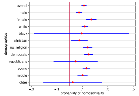
(a) homosexuality

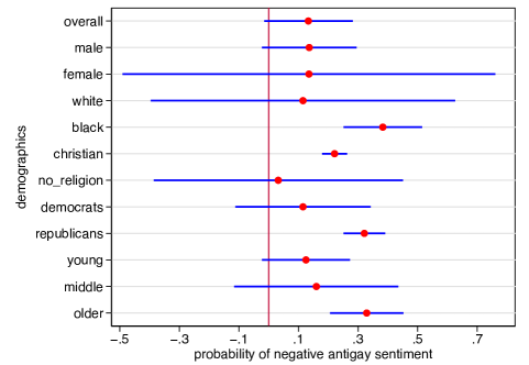
(b) antigay sentiment

Note: The red dots and the blue lines represent point estimates and their 95% confidence intervals, respectively.

5 Conclusions

This article studies the eliciting of information from sensitive survey questions. We make two main points in the paper. First, it is necessary to test the assumptions of the widely used LE before applying the method to obtain estimates about sensitive information. We prove that the assumptions of LE can be tested rigorously. We find that they are violated in the majority of empirical studies. That violation implies invalidity of LE and problematic conclusions based on using the method. Second, information can be elicited from sensitive survey questions by applying our proposed technique. To implement it, one would ask all of the respondents to answer three or more survey questions related to the information to be elicited. Random assignment of groups is not necessary. Our technique also can address measurement error in arbitrary forms, and it allows us to recover information at a disaggregated level. Applying our technique to survey data on the LGBT-population and LGBT-related sentiments leads to several novel findings that are obscured by using LE or other existing survey methods.

There are several avenues suggested for future research. One could apply our technique to other experimental methods with measurement error or unobserved heterogeneity: for example, the Goldberg paradigm experiments that are used to measure discrimination (see details in Bertrand and Duflo (2017)). Another possibility is to investigate how to optimally design survey questions and to collect respondents’ demographics in order to obtain the best estimate from survey responses.

Appendix

Appendix A Proofs

Proof of proposition 1.

Under Assumption 1, $\Pr(R_{0}=j)=\Pr(R_{1}=j)\equiv P(j)$ is the probability of outcome $j\in\mathcal{J}_{0}$ under respondents’ true preference. By Assumption 2, the probability of outcome $j\in\mathcal{J}_{0}$ in the control group is

$$P_{0}(j)=(1-p_{0}){P(j)}+\frac{p_{0}}{J+1},$$ (A.1)

or

$$P(j)=\frac{P_{0}(j)}{1-p_{0}}-\frac{p_{0}}{(J+1)(1-p_{0})}.$$ (A.2)

Consider the random variable $U\equiv R_{1}+X^{*}$, where $R_{1}$ and $X^{*}$ represent the outcomes for the nonsensitive and sensitive questions under respondents’ true preference, respectively. According to Assumption 2, the probability of an outcome $j\in\mathcal{J}_{1}$ in treatment group can be obtained by convolution of probability distributions:

$$P_{1}(j) =(1-p_{0})\left(\sum_{j-r_{1}\in\{0,1\}}P(R_{1}=r_{1})P(X^{*}=j-r_{1})\right)+\frac{p_{1}}{J+2}.$$ (A.3)

When $j=0$,

$$P_{1}(0)=(1-p_{1})P(0)P(X^{*}=0)+\frac{p_{1}}{J+2}=\frac{1-p_{1}}{1-p_{0}}\bigg{(}(1-\delta)P_{0}(0)-\frac{(1-\delta)p_{0}}{J+1}\bigg{)}+\frac{p_{1}}{J+2},$$ (A.4)

where $\delta=P(X^{*}=1)$. When $1\leq j<J+1$,

$$P_{1}(j) = (1-p_{1})\left(P(j)(1-\delta)+P(j-1)\delta\right)+\frac{p_{1}}{J+2}$$ (A.5)

$$= (1-p_{1})\left[\left(\frac{P_{0}(j)}{1-p_{0}}-\frac{p_{0}}{(J+1)(1-p_{0})}\right)(1-\delta)\right.$$

$$+ \left.\left(\frac{P_{0}(j-1)}{1-p_{0}}-\frac{p_{0}}{(J+1)(1-p_{0})}\right)\delta\right]+\frac{p_{1}}{J+2}$$

$$= \frac{1-p_{1}}{1-p_{0}}\left(\delta P_{0}(j-1)+(1-\delta)P_{0}(j)-\frac{p_{0}}{J+1}\right)+\frac{p_{1}}{J+2}.$$

When $j=J+1$,

$$P_{1}(J+1)=(1-p_{1})P(J)P(W=1)+\frac{p_{1}}{J+2}=\frac{1-p_{1}}{1-p_{0}}\bigg{(}\delta P_{0}(J)-\frac{\delta p_{0}}{J+1}\bigg{)}+\frac{p_{1}}{J+2}.$$ (A.6)

Proof of identification of $\delta,p_{0}$ and $p_{1}$ from equation (3).

Without loss of generality, we assume $J=3$. The cases with $J>3$ can be proved analogously.

When $J=3$, all the model restrictions are

$$P_{1}(0) = \frac{1-p_{1}}{1-p_{0}}\bigg{(}(1-\delta)P_{0}(0)-\frac{(1-\delta)p_{0}}{4}\bigg{)}+\frac{p_{1}}{5},$$

$$P_{1}(j) = \frac{1-p_{1}}{1-p_{0}}\left(\delta P_{0}(j-1)+(1-\delta)P_{0}(j)-\frac{p_{0}}{4}\right)+\frac{p_{1}}{5},j=1,2,3,$$

$$P_{1}(4) = \frac{1-p_{1}}{1-p_{0}}\bigg{(}\delta P_{0}(3)-\frac{\delta p_{0}}{4}\bigg{)}+\frac{p_{1}}{5},$$ (A.7)

where $0\leq P_{t}(j)\leq 1$,   $\sum_{j=0}^{J+t}P_{t}(j)=1$, and $t=0,1$.

Note that the five equations above are nonlinear in $\delta$, $p_{0}$ and $p_{1}$. Below we discuss sufficient but not necessary conditions under which Equation (A) sustains a solution. Since the equation is linear in $\delta$ when $j=1,2,3$, we use the equations for $j=1,2,3$ to get

$$\frac{P_{1}(3)-P_{1}(2)}{P_{1}(2)-P_{1}(1)}=\frac{(1-\delta)P_{0}(3)+(2\delta-1)P_{0}(2)-\delta P_{0}(1)}{(1-\delta)P_{0}(2)+(2\delta-1)P_{0}(1)-\delta P_{1}(0)},$$ (A.8)

which identifies $\delta$ whenever $(P_{1}(3)-P_{1}(2))\big{(}2P_{0}(1)-P_{0}(2)-P_{1}(0)\big{)}\neq(P_{1}(2)-P_{1}(1))\big{(}2P_{0}(2)-P_{0}(3)-P_{1}(1)\big{)}$. We then combine the first and last equations ($j=0,4$) and two other consecutive equations (e.g., $j=1,2$ or $j=2,3$) to obtain

$$\frac{P_{1}(4)-P_{1}(0)}{P_{1}(2)-P_{1}(1)}=\frac{\delta P_{0}(3)-(1-\delta)P_{0}(0)+(1-2\delta)p_{0}/4}{(1-\delta)P_{0}(2)+(2\delta-1)P_{0}(1)-\delta P_{1}(0)}.$$ (A.9)

The parameter $p_{0}$ is identified if $\delta\neq 1/2$. For a given identified pair $(\delta,p_{0})$, any condition in Equation (A) identifies $p_{1}$. The identified parameters under the sufficient conditions we provided are not necessarily in $[0,1]$. Therefore, Equation (A) sustains at most one solution. Our argument above can be generalized to $J>3$.

Proof of Corollary 1.

Starting from equation (1), we first calculate $\mathbb{E}(Y_{1})$.

$$\mathbb{E}(Y_{1}) = \sum_{j=0}^{J+1}P_{1}(j)j$$ (A.10)

$$= 0*\left\{\frac{1-p_{1}}{1-p_{0}}\bigg{(}(1-\delta)P_{0}(0)-\frac{(1-\delta)p_{0}}{J+1}\bigg{)}+\frac{p_{1}}{J+2}\right\}$$

$$+1*\left\{\frac{1-p_{1}}{1-p_{0}}\left(\delta P_{0}(0)+(1-\delta)P_{0}(1)-\frac{p_{0}}{J+1}\right)+\frac{p_{1}}{J+2}\right\}$$

$$\vdots$$

$$+J*\left\{\frac{1-p_{1}}{1-p_{0}}\left(\delta P_{0}(J-1)+(1-\delta)P_{0}(J)-\frac{p_{0}}{J+1}\right)+\frac{p_{1}}{J+2}\right\}$$

$$+(J+1)*\left\{\frac{1-p_{1}}{1-p_{0}}\bigg{(}\delta P_{0}(J)-\frac{\delta p_{0}}{J+1}\bigg{)}+\frac{p_{1}}{J+2}\right\}$$

$$= \frac{1-p_{1}}{1-p_{0}}\left\{\delta P_{0}(0)+(1+\delta)P_{0}(1)+\cdots(J+\delta)P_{0}(J)-(1+2+\cdots+J)\frac{p_{0}}{J+1}+\delta p_{0}\right\}$$

$$+(1+2+\cdots+J+1)\frac{p_{1}}{J+2}$$

$$= \frac{1-p_{1}}{1-p_{0}}\left\{\sum_{j=0}^{J}P_{0}(j)j+\delta\sum_{j=0}^{J}P_{0}(j)-\frac{Jp_{0}}{2}-\delta p_{0}\right\}+\frac{(J+1)p_{1}}{2}$$

$$= \frac{1-p_{1}}{1-p_{0}}\left\{\mathbb{E}(Y_{0})+\delta(1-p_{0})-\frac{Jp_{0}}{2}\right\}+\frac{(J+1)p_{1}}{2}.$$

Based on the expression above, we have

$$\mathbb{E}(Y_{1})-\mathbb{E}(Y_{0}) = \frac{1-p_{1}}{1-p_{0}}\left\{\mathbb{E}(Y_{0})-\frac{1-p_{0}}{1-p_{1}}\mathbb{E}(Y_{0})+\delta(1-p_{0})-\frac{Jp_{0}}{2}\right\}+\frac{(J+1)p_{1}}{2}$$ (A.11)

$$= \delta(1-p_{1})+\frac{p_{0}-p_{1}}{1-p_{0}}\mathbb{E}(Y_{0})-\frac{J(1-p_{1})p_{0}}{2(1-p_{0})}+\frac{J+1}{2}p_{1}.$$

Appendix B An Extension: Strategic Misreporting

In this section, we discuss an alternative misreporting strategy and its implications. We assume that all the respondents without sensitive information answer survey questions truthfully regardless of their group assignment. Respondents with sensitive information misreport with probability $p$ only if truthful reporting would cause privacy disclosure (in our case, respondents may cause privacy disclosure when $R_{1}=J$). When a respondent with sensitive information chooses to misreport, we assume that she answers no to the sensitive question. Following the notation in Proposition 1, the assumptions of strategic misreporting can be summarized as:

$$\Pr(X^{*}=1|R_{1}<J)=\delta,\hskip 5.69046pt\Pr(X^{*}=1|R_{1}=J)=\delta(1-p).$$ (B.1)

The assumption that all the respondents without sensitive information report truthfully implies that

$$\Pr(R_{0}=j)=\Pr(R_{1}=j)=P(j),\hskip 5.69046ptj\in\mathcal{J}_{0}.$$ (B.2)

Under the assumption above, only the outcomes $J$ and $J+1$ would be affected by misreporting. For $j=0,1,\cdots,j-1$, no misreporting is involved, we have

$$P_{1}(j) = \sum_{j-r_{1}\in\{0,1\}}\Pr(R_{1}=r_{1})\Pr(X^{*}=j-r_{1})$$ (B.3)

$$= \begin{cases}(1-\delta)P_{0}(0),&j=0.\\ (1-\delta)P_{0}(j)+\delta P_{0}(j-1)&j=1,2,\cdots,j-1.\end{cases}$$

When $j=J$, the outcome is determined by both truthful and mis-reporting because those who misreport choose to report $j=J$,

$$P_{1}(J)=(1-\delta)P_{0}(J)+\delta P(J-1)+\delta pP_{0}(J).$$ (B.4)

The outcome $j=J+1$ is observed only when respondents with sensitive information answer yes to all the $J$ nonsensitive questions under their true preference and decide to reveal their sensitive information even though doing so would discloses their privacy. Therefore, we have

$$P_{1}(J+1)=\delta(1-p)P_{0}(J).$$ (B.5)

Equations (B.3)-(B.5) summarize all the model restrictions under the strategic misreporting. The parameters $\delta$ and $p$ are both identified given $J\geq 1$. The proof is similar to that of equation (3), thus is omitted.

Based on the model restrictions (B.3)-(B.5), we can test LE with this misreporting strategy by using a testing procedure that is similar to Section 2.2. The testing results of the five articles as in Section 2.4 are presented in Table 4. The findings from the test are similar to that in Section 2.4. When $p\neq 0$, we reject the null hypothesis for 12 and 13 out of 19 questions at the 5% and 10% significance levels, respectively, accounting for 63% and 68%. By design, the testing results for $p=0$ is the same as that for $p_{1}=p_{2}=0$ in Section 2.4. The model is rejected for 53% (10 out of 19) and 63% (12 out of 19) of questions at the 5% and 10% significance level, respectively, in both specifications.

Table 4: Results of estimation and testing, strategic misreporting

			GMM estimate			testing results
sensitive question	sample size	mean difference	$\delta$	$p$		$p\neq 0$	$p=0$
favorable view of CCP	1576	0.057	—	—		✗	✗
		(0.057)
consider self Hong Kongese	1576	0.816	—	—		✗	✗
		(0.048)
support for HK independence	1576	0.521	0.521	0.209		$\checkmark$	✗
		(0.052)	(0.052)	(0.303)
support violence in pursuit of HK’s political rights	1576	0.389	0.423	—		✗	$\checkmark$
		(0.048)	(0.052)
I completely trust the central government of China	1807	0.290	—	—		✗	✗
		(0.038)
do you consider yourself to be heterosexual?	2516	0.894	—	—		✗	$\dagger$
		(0.036)
are you sexually attracted to members of the same sex?	2516	0.258	—	—		$\dagger$	$\dagger$
		(0.035)
have you had a sexual experience with someone of the same sex?	2516	0.545	—	—		✗	✗
		(0.040)
do you think marriages between gay and lesbian couples should be recognized by the law as valid, with the same rights as heterosexual marriages?	2516	0.986	—	—		✗	✗
		(0.032)
would you be happy to have an openly lesbian, gay, or bisexual manager at work?	2516	0.912	—	—		✗	✗
		(0.038)
do you believe it should be illegal to discriminate in hiring based on someone’s sexual orientation?	2516	0.806	—	—		✗	✗
		(0.031)
do you believe lesbians and gay men should be allowed to adopt children?	2516	0.878	—	—		✗	✗
		(0.034)
do you think someone who is homosexual can change their sexual orientation if they choose to do so?	2516	0.186	0.187	—		$\checkmark$	$\checkmark$
		(0.034)	(0.031)
w/o smartcards system, members of this household have been asked by officials to lie about the amount of work they did on NREGS	917	0.044	0.014	—		$\checkmark$	$\checkmark$
		(0.059)	(0.072)
w/o smartcards system, members of this household have been given the chance to meet with the CM of AP to discuss problems with NREGS?	897	0.174	0.133	0.275		$\checkmark$	✗
		(0.062)	(0.088)	(0.233)
w/ smartcards system, members of this household have been asked by officials to lie about the amount of work they did on NREGS	2300	0.106	—	—		✗	✗
		(0.036)
w/ smartcards system, members of this household have been given the chance to meet with the CM of AP to discuss problems with NREGS?	2276	0.154	0.140	—		$\checkmark$	$\checkmark$
		(0.037)	(0.053)
treated voters differently by religion/caste	3833	0.242	0.248	—		$\checkmark$	$\checkmark$
		(0.027)	(0.029)
attempted to influence voting	3850	0.142	—	—		✗	✗
		(0.038)

• Note: The five panels (from top to bottom) are results for Cantoni et al. (2019), Chen and Yang (2019), Coffman et al. (2017), Muralidharan et al. (2016), and Neggers (2018), respectively.

• ✗, $\dagger$, and $\checkmark$ indicate $p<0.05$, $p<0.1$, and $p>0.1$, respectively. Standard errors in parentheses are bootstrapped $1000$ times. When only $\hat{\delta}$ is provided, then $p=0$; if both $\hat{\delta}$ and $\hat{p}$ are provided, then $p\neq 0$.

Appendix C Estimation

In this section, we propose three methods to estimate the model primitives identified in Theorem 1. The first two methods are nonparametric and follow the identification procedure closely. The third one utilizes maximum likelihood estimation (MLE) to estimate the model primitives. The data sample is represented by $\{X_{ji},Z_{i}\},j=1,2,3,i=1,2,\cdots,n$, based on the $n$ respondents’ answers to three questions ($X_{ji}$) and their characteristics ($Z_{i}$).

C.1 Discrete covariates

When the vector of covariates $Z$ takes only a few discrete values, such as gender, political affiliation, and race, it is convenient to estimate the model using a nonparametric approach based on the identification procedure. According to the main identification equation (14), the eigenvector matrix $M_{X_{1}|X^{*},z}$ can be written as a function of the observed matrix $M_{X_{1},x_{2},X_{3}|z}M^{-1}_{X_{1},X_{3}|z}$,

$$M_{X_{1}|X^{*},z}=\psi(M_{X_{1},x_{2},X_{3}|z}M^{-1}_{X_{1},X_{3}|z}),$$

where $\psi(\cdot)$ is a function determined by eigenvalue-eigenvector decomposition of a matrix. Thus, we estimate $M_{X_{1}|X^{*},z}$ as

$$\widehat{M}_{X_{1}|X^{*},z}=\psi(\widehat{M}_{X_{1},x_{2},X_{3}|z}\widehat{M}^{-1}_{X_{1},X_{3}|z}),$$ (C.1)

where $\widehat{M}_{X_{1},x_{2},X_{3}|z}$ and $\widehat{M}^{-1}_{X_{1},X_{3}|z}$ can be estimated by

$$\left(\widehat{M}_{X_{1},x_{2},X_{3}|z}\right)_{l,k}=\sum\nolimits_{i=1}^{n}\mathbbm{1}\left(X_{1i}=l-1,X_{2i}=x_{2},X_{3i}=k-1\right)\mathbbm{1}\left(Z_{i}=z\right)/\sum\nolimits_{i=1}^{n}\mathbbm{1}\left(Z_{i}=z\right)$$ (C.2)

for $k,l=1,2$. The matrix $\widehat{M}_{X_{1},X_{3}|z}$ is estimated analogously. Once $\widehat{M}_{X_{1}|X^{*},z}$ is obtained, we follow equation (15) to estimate $\Pr(X^{*}|z)\equiv[\Pr(X^{*}=0|z)\hskip 8.5359pt\Pr(X^{*}=1|z)]^{\prime}$,

$$\widehat{\Pr}(X^{*}|z)=\widehat{M}^{-1}_{X_{1}|X^{*},z}\left[\widehat{\Pr}(X_{1}=0|z)\hskip 8.5359pt\widehat{\Pr}(X_{1}=1|z)\right]^{\prime},$$ (C.3)

where $\widehat{\Pr}(X_{1}=j|z)=\sum\nolimits_{i=1}^{n}\mathbbm{1}\left(X_{1i}=j,Z_{i}=z\right)/\sum\nolimits_{i=1}^{n}\mathbbm{1}\left(Z_{i}=z\right),j=0,1.$

The matrix $M_{X_{3}|X^{*},z}$ can be estimated from equation (13) and the relationship $M_{X_{3},X^{*}|z}=M_{X_{3}|X^{*},z}M_{X^{*}|z}$, where $M_{X^{*}|z}$ is a diagonal matrix and the two diagonal elements are $\Pr(X^{*}=0|z)$ and $\Pr(X^{*}=1|z)$. Thus, we have

$$\widehat{M}_{X_{3}|X^{*},z}=\left(\widehat{M}^{-1}_{X_{1}|X^{*},z}\widehat{M}_{X_{1},X_{3}|z}\right)^{\prime}\hbox{diag}\left[1/\widehat{\Pr}(X^{*}=0|z)\hskip 8.5359pt1/\widehat{\Pr}(X^{*}=1|z)\right].$$ (C.4)

The main advantage of the nonparametric estimation is that it is global and involves no optimization. However, the estimated probability might be outside the interval $[0,1]$ due to finite sample properties. To address this potential issue, we propose an extreme estimator with probabilities constrained to $[0,1]$ based on equation (14). Let $p_{1k}=\Pr(X_{1}=1|X^{*}=k,z)$ and $p_{2k}=\Pr(X_{2}=x_{2}|X^{*}=k,z)$ be the parameters to be estimated for $k=0,1$. We assume that Assumption 4(ii) holds for $X_{1}$ such that $p_{10}<p_{11}$. The estimation problem becomes

$$\left(\widehat{p}_{10},\widehat{p}_{11},\widehat{p}_{20},\widehat{p}_{21}\right) = \arg\min\left|\left|\widehat{M}_{X_{1},x_{2},X_{3}|z}\widehat{M}^{-1}_{X_{1},X_{3}|z}-MDM^{-1}(p_{10},p_{11},p_{20},p_{21},z)\right|\right|$$

subject to $$(i)\hskip 2.84544pt(p_{10},p_{11},p_{20},p_{21})\in[0,1]^{4}$$ (C.5)

$$(ii)\hskip 2.84544ptp_{20}\neq p_{21}$$

$$(iii)\hskip 2.84544ptp_{10}<p_{11},$$

where the $\left|\left|\cdot\right|\right|$ is a matrix norm (e.g., Frobenius norm) and the constraints are imposed according to Assumption 4. Analogously, $\Pr(X^{*}|z)$ and $\Pr(X_{3}|X^{*},z)$ are estimated from equation (15) and (13), respectively.

C.2 Continuous convariates

When the vector of characteristics $Z$ takes a large number of values or is continuous, the nonparametric estimation demands a large sample, which is often unavailable. In this section, we present an MLE method to estimate the latent probabilities.

The MLE is based on the main identification equation (14),

$$\Pr\left(X_{1},X_{2},X_{3}|z\right)=\sum\nolimits_{X^{*}\in\{0,1\}}\Pr\left(X_{1}|X^{*},z\right)\Pr\left(X_{2}|X^{*},z\right)\Pr\left(X_{3}|X^{*},z\right)\Pr\left(X^{*}|z\right).$$

We first parametrize the unknown probabilities.

$$\Pr(X_{1}=1|X^{*}=j,z) \equiv g(z;\alpha_{j}),\hskip 8.5359pt\Pr(X_{2}=1|X^{*}=j,z)\equiv g(z;\beta_{j}),$$

$$\Pr(X_{3}=1|X^{*}=j,z) \equiv g(z;\gamma_{j}),\hskip 8.5359pt\Pr(X^{*}=1|z)\equiv g(z;\rho),j=0,1.$$ (C.6)

The $g(\cdot)$ can take various functional forms such as a logistic function. The model parameters $(\alpha_{0},\alpha_{1},\beta_{0},\beta_{1},\gamma_{0},\gamma_{1},\rho)$ are estimated by maximizing the following log-likelihood function.

$$\log\mathcal{L} = \sum\nolimits_{i=1}^{n}\log\left\{\sum\nolimits_{X^{*}\in\{0,1\}}\Pr\left(X_{1i}|X^{*},z_{i}\right)\Pr\left(X_{2i}|X^{*},z_{i}\right)\Pr\left(X_{3i}|X^{*},z_{i}\right)\Pr\left(X^{*}|z_{i}\right)\right\}.$$ (C.7)

$$= \sum\nolimits_{i=1}^{n}\log\bigg{\{}\sum\nolimits_{j\in\{0,1\}}\big{[}g(z_{i};\alpha_{j})\big{]}^{X_{1i}}\big{[}1-g(z_{i};\alpha_{j})\big{]}^{1-X_{1i}}\big{[}g(z_{i};\beta_{j})\big{]}^{X_{2i}}\big{[}1-g(z_{i};\beta_{j})\big{]}^{1-X_{2i}}$$

$$\times\big{[}g(z_{i};\gamma_{j})\big{]}^{X_{3i}}\big{[}1-g(z_{i};\gamma_{j})\big{]}^{1-X_{3i}}g(z_{i};\rho)^{j}\big{[}1-g(z_{i};\rho)\big{]}^{1-j}{\color[rgb]{1,1,1}\{\sum_{j\in\{0,1\}}}\bigg{\}},$$

Assumption 4(ii) requires $\Pr(X_{1}=1|X^{*}=0,z)<\Pr(X_{1}=1|X^{*}=1,z)$, which implies that $\alpha_{0}\neq\alpha_{1},\beta_{0}\neq\beta_{1},\gamma_{0}\neq\gamma_{1},$ and $g(z;\alpha_{0})<g(z;\alpha_{1})$ for all $z$ are needed for identification.

Appendix D Monte Carlo Experiments

In this section, we provide Monte Carlo evidence to illustrate the performance of our proposed methodology. We consider two settings where the covariate $Z$ is discrete and continuous, respectively. The sample size is set to be 500, 1,000, and 2,000, which is comparable to the sample size in the articles we analyze in section 2.4. The results are based on 1,000 replications.

In the first setting, $Z$ is a binary variable with the probability of $Z=0$ being 0.4. We set parameters for $\Pr(X^{*}=1|z)$ and $\Pr(X_{j}=1|x^{*},z)$ to generate the sample $\{X_{1i},X_{2i},X_{3i},Z_{i}\},n=1,2,\cdots,n.$ The first step of estimation is to test the rank of the $2\times 2$ matrix $M_{X_{1},X_{3}|z}$ by using the sequential testing procedure proposed in Robin and Smith (2000). Specifically, we test

$$H_{0}:rank\left(M_{X_{1},X_{3}|z}\right)=1\hskip 8.5359ptvs.\hskip 8.5359ptH_{1}:rank\left(M_{X_{1},X_{3}|z}\right)>1.$$

We reject the null hypothesis with a 100% rejection rate for all the three sample sizes. Next, we estimate the parameters $\Pr(X^{*}),\Pr(X^{*}|z)$, and $\Pr(X_{j}|x^{*},z)$ using the method of matrix decomposition and the extreme estimator with a Frobenius norm. The estimated results are presented in Table 5. As shown in the table, our estimates track the true value closely even for a small sample size $n=500$. As sample size increases, the standard error decreases significantly. The performance of the closed-form estimator and the extreme estimator is similar.

In the second setting, $Z$ is uniformly distributed on $[0,1]$. The data generating process is based on Equation (C.2) with $g(\cdot)$ being a logistic function. From the model primitives, we generate the joint distribution of $\{X_{1i},X_{2i},X_{3i},Z_{i}\}$ for $i=1,2,\cdots,n$. We present the estimation results in Table 6. The results show good performance of our estimation method. The estimates improve significantly when sample size increases from $500$ to $2,000$.

A comparison of the results using the nonparametric methods and MLE shows that the nonparametric approach performs better than MLE, especially when the sample size is relatively small, e.g., $n=500$. This is mainly due to the fact that the nonparametric method is global and the estimation involves no optimization. Specifically, a closed-form estimator is global by construction. By contrast, an optimization algorithm, such as MLE, can only guarantee a local maximum or minimum even when a global solution exists. The nonparametric approach also allows us to analyze how parameters affect the estimate constructively while this can only be done numerically for an estimator using optimization algorithms. In addition, a closed-form estimator is computationally more convenient since most of the optimization algorithms involve iterations.

In the second set of simulation, we check the sensitivity of our estimates to the assumption of conditional independence, Assumption 3. We allow mutual correlation between $X_{j}$ and $X_{k}$ conditional on $X^{*}$ and $Z$ by assuming the correlation coefficients for any pair of $X$ is a constant $\sigma$. Then we investigate how our estimate depends on $\sigma$. We present the results of estimation for a discrete $Z$ in Tables 7-9 and a continuous $Z$ in table 10. For a model with a discrete $Z$, the estimates for $\sigma=0.05$ and $\sigma=0.10$ are close to $\sigma=0$. When $\sigma=0.05$, the estimates are very close to the true values, especially when the sample size is 2000. Not surprisingly, when the correlation coefficient increases to $\sigma=0.2$, the bias becomes larger in magnitude. Correlation leads to overestimation. The impact of the correlation is larger for a continuous $Z$. Table 10 shows that the estimates are close to the no correlation case only for $\sigma=0.05$.

Table 5: Simulation results of nonparametric estimation: discrete $Z$

		estimate: closed-form				estimate: extreme estimator
parameter	true value	$n=500$	$n=1000$	$n=2000$		$n=500$	$n=1000$	$n=2000$
$\Pr(X^{*}=1)$	0.642	0.643	0.641	0.634		0.641	0.642	0.634
		(0.062)	(0.042)	(0.029)		(0.076)	(0.044)	(0.031)
$\Pr(X^{*}=1|z=0)$	0.378	0.377	0.376	0.379		0.382	0.377	0.379
		(0.102)	(0.071)	(0.050)		(0.103)	(0.071)	(0.052)
$\Pr(X^{*}=1|z=1)$	0.818	0.808	0.813	0.817		0.803	0.813	0.817
		(0.082)	(0.049)	(0.034)		(0.108)	(0.055)	(0.036)
$\Pr(X_{1}=1|X^{*}=0,z=0)$	0.269	0.265	0.270	0.267		0.264	0.268	0.267
		(0.079)	(0.058)	(0.037)		(0.086)	(0.057)	(0.040)
$\Pr(X_{1}=1|X^{*}=0,z=1)$	0.310	0.288	0.303	0.304		0.297	0.305	0.304
		(0.191)	(0.112)	(0.073)		(0.151)	(0.105)	(0.073)
$\Pr(X_{1}=1|X^{*}=1,z=0)$	0.881	0.895	0.885	0.882		0.880	0.881	0.881
		(0.113)	(0.076)	(0.051)		(0.078)	(0.062)	(0.048)
$\Pr(X_{1}=1|X^{*}=1,z=1)$	0.900	0.904	0.903	0.900		0.904	0.902	0.900
		(0.040)	(0.025)	(0.017)		(0.046)	(0.030)	(0.018)
$\Pr(X_{2}=1|X^{*}=0,z=0)$	0.269	0.266	0.270	0.268		0.267	0.269	0.267
		(0.061)	(0.048)	(0.032)		(0.065)	(0.047)	(0.034)
$\Pr(X_{2}=1|X^{*}=0,z=1)$	0.289	0.285	0.288	0.287		0.285	0.288	0.287
		(0.120)	(0.080)	(0.055)		(0.125)	(0.084)	(0.055)
$\Pr(X_{2}=1|X^{*}=1,z=0)$	0.731	0.735	0.734	0.732		0.734	0.735	0.733
		(0.085)	(0.062)	(0.041)		(0.083)	(0.060)	(0.040)
$\Pr(X_{2}=1|X^{*}=1,z=1)$	0.750	0.752	0.752	0.750		0.755	0.753	0.751
		(0.038)	(0.026)	(0.019)		(0.053)	(0.031)	(0.019)
$\Pr(X_{3}=1|X^{*}=0,z=0)$	0.269	0.262	0.266	0.267		0.259	0.264	0.267
		(0.077)	(0.056)	(0.037)		(0.071)	(0.050)	(0.036)
$\Pr(X_{3}=1|X^{*}=0,z=1)$	0.289	0.256	0.283	0.284		0.285	0.285	0.283
		(0.212)	(0.107)	(0.076)		(0.169)	(0.116)	(0.087)
$\Pr(X_{3}=1|X^{*}=1,z=0)$	0.881	0.899	0.893	0.884		0.880	0.888	0.883
		(0.110)	(0.080)	(0.050)		(0.100)	(0.069)	(0.052)
$\Pr(X_{3}=1|X^{*}=1,z=1)$	0.891	0.896	0.893	0.892		0.892	0.893	0.892
		(0.045)	(0.026)	(0.018)		(0.062)	(0.030)	(0.018)

Table 6: Simulation results: continuous $Z$

		estimate
parameter	true value	$n=500$	$n=1000$	$n=2000$
$\rho$	1	0.964	0.989	0.985
		(0.396)	(0.273)	(0.193)
$\alpha_{1}$	1	1.021	1.012	1.008
		(0.267)	(0.188)	(0.126)
$\alpha_{0}$	-1	-1.031	-1.018	-0.990
		(0.469)	(0.292)	(0.201)
$\beta_{1}$	2	2.272	2.050	2.036
		(1.575)	(0.360)	(0.249)
$\beta_{0}$	-2	-2.494	-2.144	-2.044
		(2.859)	(0.723)	(0.436)
$\gamma_{1}$	2	2.286	2.050	2.030
		(2.235)	(0.378)	(0.240)
$\gamma_{0}$	-2	-2.446	-2.107	-2.031
		(2.099)	(0.694)	(0.443)

Table 7: Simulation results of nonparametric estimation: discrete $Z$, $\sigma=0.05$

		estimate: closed-form				estimate: extreme estimator
parameter	true value	$n=500$	$n=1000$	$n=2000$		$n=500$	$n=1000$	$n=2000$
$\Pr(X^{*}=1|z=0)$	0.378	0.394	0.387	0.389		0.397	0.388	0.389
		(0.097)	(0.068)	(0.045)		(0.093)	(0.067)	(0.045)
$\Pr(X*=1|z=1)$	0.818	0.814	0.817	0.819		0.813	0.816	0.819
		(0.074)	(0.046)	(0.031)		(0.073)	(0.046)	(0.031)
$\Pr(X^{*}=1)$	0.642	0.659	0.648	0.647		0.660	0.648	0.647
		(0.060)	(0.039)	(0.026)		(0.059)	(0.039)	(0.026)
$\Pr(X_{1}=1|X^{*}=0,z=0)$	0.269	0.246	0.254	0.254		0.248	0.255	0.254
		(0.076)	(0.051)	(0.035)		(0.075)	(0.051)	(0.035)
$\Pr(X_{1}=1|X^{*}=0,z=1)$	0.310	0.273	0.289	0.293		0.279	0.289	0.293
		(0.165)	(0.101)	(0.070)		(0.143)	(0.099)	(0.070)
$\Pr(X_{1}=1|X^{*}=1,z=0)$	0.881	0.896	0.889	0.886		0.884	0.887	0.886
		(0.108)	(0.066)	(0.045)		(0.082)	(0.061)	(0.044)
$\Pr(X_{1}=1|X^{*}=1,z=1)$	0.900	0.903	0.903	0.901		0.903	0.904	0.901
		(0.039)	(0.024)	(0.016)		(0.037)	(0.024)	(0.016)
$\Pr(X_{2}=1|X^{*}=0,z=0)$	0.269	0.240	0.243	0.245		0.242	0.244	0.245
		(0.062)	(0.043)	(0.030)		(0.065)	(0.043)	(0.030)
$\Pr(X_{2}=1|X^{*}=0,z=1)$	0.289	0.259	0.262	0.265		0.258	0.262	0.265
		(0.110)	(0.076)	(0.053)		(0.110)	(0.076)	(0.053)
$\Pr(X_{2}=1|X^{*}=1,z=0)$	0.731	0.719	0.721	0.719		0.717	0.720	0.719
		(0.083)	(0.058)	(0.039)		(0.082)	(0.058)	(0.039)
$\Pr(X_{2}=1|X^{*}=1,z=1)$	0.750	0.743	0.746	0.744		0.744	0.746	0.744
		(0.039)	(0.026)	(0.019)		(0.045)	(0.026)	(0.019)
$\Pr(X_{3}=1|X^{*}=0,z=0)$	0.269	0.238	0.242	0.245		0.235	0.242	0.245
		(0.074)	(0.050)	(0.034)		(0.070)	(0.049)	(0.034)
$\Pr(X_{3}=1|X^{*}=0,z=1)$	0.289	0.240	0.259	0.261		0.254	0.259	0.261
		(0.180)	(0.105)	(0.067)		(0.144)	(0.103)	(0.067)
$\Pr(X_{3}=1|X^{*}=1,z=0)$	0.881	0.872	0.875	0.868		0.866	0.873	0.868
		(0.102)	(0.068)	(0.047)		(0.083)	(0.063)	(0.046)
$\Pr(X_{3}=1|X^{*}=1,z=1)$	0.891	0.889	0.888	0.888		0.889	0.888	0.888
		(0.042)	(0.025)	(0.018)		(0.037)	(0.025)	(0.018)

Table 8: Simulation results of nonparametric estimation: discrete $Z$, $\sigma=0.10$

		estimate: closed-form				estimate: extreme estimator
parameter	true value	$n=500$	$n=1000$	$n=2000$		$n=500$	$n=1000$	$n=2000$
$\Pr(X^{*}=1|z=0)$	0.378	0.406	0.400	0.402		0.406	0.401	0.402
		(0.089)	(0.060)	(0.042)		(0.086)	(0.059)	(0.042)
$\Pr(X*=1|z=1)$	0.818	0.821	0.825	0.824		0.819	0.825	0.824
		(0.057)	(0.041)	(0.028)		(0.057)	(0.041)	(0.028)
$\Pr(X^{*}=1)$	0.642	0.650	0.660	0.658		0.819	0.825	0.824
		(0.050)	(0.034)	(0.024)		(0.057)	(0.041)	(0.028)
$\Pr(X_{1}=1|X^{*}=0,z=0)$	0.269	0.237	0.241	0.238		0.235	0.241	0.238
		(0.088)	(0.049)	(0.035)		(0.073)	(0.049)	(0.035)
$\Pr(X_{1}=1|X^{*}=0,z=1)$	0.310	0.261	0.266	0.276		0.267	0.267	0.276
		(0.159)	(0.106)	(0.071)		(0.131)	(0.103)	(0.071)
$\Pr(X_{1}=1|X^{*}=1,z=0)$	0.881	0.891	0.890	0.887		0.888	0.888	0.887
		(0.097)	(0.062)	(0.040)		(0.075)	(0.058)	(0.040)
$\Pr(X_{1}=1|X^{*}=1,z=1)$	0.900	0.904	0.903	0.902		0.904	0.903	0.902
		(0.031)	(0.023)	(0.015)		(0.033)	(0.023)	(0.015)
$\Pr(X_{2}=1|X^{*}=0,z=0)$	0.269	0.217	0.217	0.217		0.216	0.217	0.217
		(0.067)	(0.040)	(0.027)		(0.060)	(0.041)	(0.027)
$\Pr(X_{2}=1|X^{*}=0,z=1)$	0.289	0.232	0.236	0.238		0.232	0.236	0.238
		(0.102)	(0.072)	(0.050)		(0.102)	(0.073)	(0.050)
$\Pr(X_{2}=1|X^{*}=1,z=0)$	0.731	0.709	0.710	0.706		0.710	0.710	0.706
		(0.086)	(0.053)	(0.037)		(0.080)	(0.053)	(0.037)
$\Pr(X_{2}=1|X^{*}=1,z=1)$	0.750	0.736	0.734	0.735		0.737	0.734	0.735
		(0.036)	(0.027)	(0.018)		(0.040)	(0.027)	(0.018)
$\Pr(X_{3}=1|X^{*}=0,z=0)$	0.269	0.218	0.219	0.218		0.214	0.219	0.218
		(0.079)	(0.047)	(0.031)		(0.065)	(0.046)	(0.031)
$\Pr(X_{3}=1|X^{*}=0,z=1)$	0.289	0.223	0.225	0.232		0.234	0.227	0.232
		(0.149)	(0.101)	(0.065)		(0.129)	(0.098)	(0.065)
$\Pr(X_{3}=1|X^{*}=1,z=0)$	0.881	0.857	0.856	0.851		0.856	0.856	0.851
		(0.100)	(0.060)	(0.043)		(0.082)	(0.059)	(0.043)
$\Pr(X_{3}=1|X^{*}=1,z=1)$	0.891	0.885	0.882	0.882		0.885	0.882	0.882
		(0.035)	(0.025)	(0.017)		(0.034)	(0.025)	(0.017)

Table 9: Simulation results of nonparametric estimation: discrete $Z$, $\sigma=0.20$

		estimate: closed-form				estimate: extreme estimator
parameter	true value	$n=500$	$n=1000$	$n=2000$		$n=500$	$n=1000$	$n=2000$
$\Pr(X^{*}=1|z=0)$	0.378	0.428	0.427	0.428		0.428	0.427	0.428
		(0.070)	(0.049)	(0.034)		(0.069)	(0.049)	(0.034)
$\Pr(X*=1|z=1)$	0.818	0.829	0.832	0.831		0.827	0.831	0.831
		(0.050)	(0.034)	(0.024)		(0.052)	(0.035)	(0.024)
$\Pr(X^{*}=1)$	0.642	0.667	0.672	0.667		0.666	0.672	0.667
		(0.042)	(0.029)	(0.019)		(0.042)	(0.029)	(0.019)
$\Pr(X_{1}=1|X^{*}=0,z=0)$	0.269	0.206	0.208	0.209		0.206	0.208	0.209
		(0.063)	(0.044)	(0.031)		(0.063)	(0.044)	(0.031)
$\Pr(X_{1}=1|X^{*}=0,z=1)$	0.310	0.234	0.238	0.247		0.243	0.240	0.247
		(0.151)	(0.102)	(0.061)		(0.123)	(0.093)	(0.061)
$\Pr(X_{1}=1|X^{*}=1,z=0)$	0.881	0.895	0.891	0.888		0.892	0.890	0.888
		(0.071)	(0.048)	(0.033)		(0.065)	(0.048)	(0.033)
$\Pr(X_{1}=1|X^{*}=1,z=1)$	0.900	0.903	0.903	0.903		0.904	0.903	0.903
		(0.030)	(0.020)	(0.014)		(0.033)	(0.021)	(0.014)
$\Pr(X_{2}=1|X^{*}=0,z=0)$	0.269	0.155	0.156	0.155		0.155	0.156	0.155
		(0.050)	(0.034)	(0.025)		(0.050)	(0.034)	(0.025)
$\Pr(X_{2}=1|X^{*}=0,z=1)$	0.289	0.177	0.185	0.183		0.178	0.184	0.183
		(0.090)	(0.063)	(0.044)		(0.089)	(0.063)	(0.044)
$\Pr(X_{2}=1|X^{*}=1,z=0)$	0.731	0.680	0.678	0.679		0.680	0.678	0.679
		(0.069)	(0.050)	(0.034)		(0.069)	(0.050)	(0.034)
$\Pr(X_{2}=1|X^{*}=1,z=1)$	0.750	0.718	0.717	0.717		0.718	0.717	0.717
		(0.035)	(0.024)	(0.017)		(0.038)	(0.026)	(0.017)
$\Pr(X_{3}=1|X^{*}=0,z=0)$	0.269	0.157	0.158	0.159		0.156	0.158	0.159
		(0.059)	(0.039)	(0.028)		(0.057)	(0.039)	(0.028)
$\Pr(X_{3}=1|X^{*}=0,z=1)$	0.289	0.154	0.165	0.172		0.175	0.169	0.172
		(0.203)	(0.093)	(0.065)		(0.119)	(0.086)	(0.065)
$\Pr(X_{3}=1|X^{*}=1,z=0)$	0.881	0.826	0.824	0.822		0.825	0.824	0.822
		(0.079)	(0.050)	(0.037)		(0.076)	(0.050)	(0.037)
$\Pr(X_{3}=1|X^{*}=1,z=1)$	0.891	0.875	0.873	0.874		0.875	0.873	0.874
		(0.034)	(0.023)	(0.016)		(0.033)	(0.023)	(0.016)

Table 10: Simulation results: continuous $Z$ with correlation

		$\sigma=0.05$				$\sigma=0.10$				$\sigma=0.20$
parameter	true value	$500$	$1000$	$2000$		$500$	$1000$	$2000$		$500$	$1000$	$2000$
$\rho$	1	1.015	1.017	1.028		1.053	1.065	1.071		1.078	1.104	1.106
		(0.365)	(0.268)	(0.187)		(0.354)	(0.238)	(0.180)		(0.309)	(0.202)	(0.141)
$\alpha_{1}$	1	1.044	1.037	1.034		1.074	1.059	1.066		1.143	1.118	1.125
		(0.259)	(0.183)	(0.126)		(0.243)	(0.173)	(0.124)		(0.231)	(0.170)	(0.116)
$\alpha_{0}$	-1	-1.106	-1.086	-1.083		-1.215	-1.213	-1.195		-1.462	-1.417	-1.400
		(0.424)	(0.303)	(0.211)		(0.448)	(0.301)	(0.202)		(0.469)	(0.304)	(0.211)
$\beta_{1}$	2	2.068	1.997	1.954		1.976	1.896	1.882		1.835	1.761	1.757
		(0.889)	(0.342)	(0.212)		(0.671)	(0.289)	(0.208)		(0.465)	(0.269)	(0.176)
$\beta_{0}$	-2	-2.740	-2.446	-2.335		-3.184	-2.794	-2.731		-4.484	-3.895	-3.698
		(2.109)	(0.914)	(0.495)		(2.645)	(0.846)	(0.556)		(6.401)	(1.651)	(0.755)
$\gamma_{1}$	2	2.071	1.999	1.959		2.003	1.889	1.868		1.849	1.766	1.748
		(0.780)	(0.372)	(0.216)		(0.811)	(0.288)	(0.193)		(0.804)	(0.245)	(0.169)
$\gamma_{0}$	-2	-2.725	-2.398	-2.340		-3.187	-2.816	-2.703		-4.972	-3.896	-3.687
		(2.019)	(0.822)	(0.501)		(2.633)	(0.886)	(0.590)		(9.221)	(1.254)	(0.781)

References

- (1)
- Andrew et al. (1993) Andrew, Alan L, K-W Eric Chu, and Peter Lancaster, “Derivatives of eigenvalues and eigenvectors of matrix functions,” SIAM journal on matrix analysis and applications, 1993, 14 (4), 903–926.
- Andrews and Shi (2017) Andrews, Donald WK and Xiaoxia Shi, “Inference based on many conditional moment inequalities,” Journal of Econometrics, 2017, 196 (2), 275–287.
- Barrera et al. (2020) Barrera, Oscar, Sergei Guriev, Emeric Henry, and Ekaterina Zhuravskaya, “Facts, alternative facts, and fact checking in times of post-truth politics,” Journal of Public Economics, 2020, 182, 104123.
- Bertrand and Duflo (2017) Bertrand, Marianne and Esther Duflo, “Field experiments on discrimination,” in “Handbook of economic field experiments,” Vol. 1, Elsevier, 2017, pp. 309–393.
- Bilir et al. (2019) Bilir, L Kamran, Davin Chor, and Kalina Manova, “Host-country financial development and multinational activity,” European Economic Review, 2019, 115, 192–220.
- Blair et al. (2018) Blair, Graeme, Alexander Coppock, and Margaret Moor, “When to worry about sensitivity bias: evidence from 30 years of list experiments,” Working Paper, University of California, Los Angeles, 2018.
- Blair and Imai (2012) and Kosuke Imai, “Statistical Analysis of List Experiments,” Political Analysis, 2012, 20, 47–77.
- Blair et al. (2019) , Winston Chou, and Kosuke Imai, “List experiments with measurement error,” Political Analysis, 2019, 27 (4), 455–480.
- Blattman et al. (2017) Blattman, Christopher, Julian C Jamison, and Margaret Sheridan, “Reducing crime and violence: Experimental evidence from cognitive behavioral therapy in Liberia,” American Economic Review, 2017, 107 (4), 1165–1206.
- Blattman et al. (2016) , Julian Jamison, Tricia Koroknay-Palicz, Katherine Rodrigues, and Margaret Sheridan, “Measuring the measurement error: A method to qualitatively validate survey data,” Journal of Development Economics, 2016, 120, 99–112.
- Bollinger (1998) Bollinger, C.R., “Measurement error in the current population survey: A nonparametric look,” Journal of Labor Economics, 1998, 16 (3), 576–594.
- Bound et al. (2001) Bound, John, Charles Brown, and Nancy Mathiowetz, “Measurement error in survey data,” in “Handbook of econometrics,” Vol. 5, Elsevier, 2001, pp. 3705–3843.
- Cantoni et al. (2019) Cantoni, Davide, David Y Yang, Noam Yuchtman, and Y Jane Zhang, “Protests as strategic games: experimental evidence from Hong Kong’s anti-authoritarian movement,” The Quarterly Journal of Economics, 2019, 134 (2), 1021–1077.
- Chen et al. (2005) Chen, X., H. Hong, and E. Tamer, “Measurement error models with auxiliary data,” Review of Economic Studies, 2005, 72 (2), 343–366.
- Chen and Yang (2019) Chen, Yuyu and David Y Yang, “The impact of media censorship: 1984 or brave new world?,” American economic review, 2019, 109 (6), 2294–2332.
- Chong et al. (2013) Chong, Alberto, Marco Gonzalez-Navarro, Dean Karlan, and Martin Valdivia, “Effectiveness and spillovers of online sex education: Evidence from a randomized evaluation in Colombian public schools,” NBER Working Paper Series, 2013, p. 18776.
- Coffman et al. (2017) Coffman, Katherine B, Lucas C Coffman, and Keith M Marzilli Ericson, “The size of the LGBT population and the magnitude of antigay sentiment are substantially underestimated,” Management Science, 2017, 63 (10), 3168–3186.
- Feng and Hu (2013) Feng, Shuaizhang and Yingyao Hu, “Misclassification errors and the underestimation of the US unemployment rate,” American Economic Review, 2013, 103 (2), 1054–70.
- Gonsiorek et al. (1995) Gonsiorek, John C, Randall L Sell, and James D Weinrich, “Definition and measurement of sexual orientation,” Suicide and Life-Threatening Behavior, 1995, 25, 40–51.
- Gosen (2014) Gosen, Stefanie, “Social desirability in survey research: Can the list experiment provide the truth?,” Ph.D. Dissertation, Philipps-Universität, Marburg, 2014.
- Haushofer and Shapiro (2016) Haushofer, Johannes and Jeremy Shapiro, “The short-term impact of unconditional cash transfers to the poor: experimental evidence from Kenya,” Quarterly Journal of Economics, 2016, 131 (4), 1973–2042.
- Hu (2008) Hu, Yingyao, “Identification and estimation of nonlinear models with misclassification error using instrumental variables: A general solution,” Journal of Econometrics, 2008, 144 (1), 27–61.
- Hu (2017) , “The econometrics of unobservables: Applications of measurement error models in empirical industrial organization and labor economics,” Journal of econometrics, 2017, 200 (2), 154–168.
- Humphreys et al. (2019) Humphreys, Macartan, Raul Sanchez de la Sierra, and Peter Van der Windt, “Exporting democratic practices: Evidence from a village governance intervention in Eastern Congo,” Journal of Development Economics, 2019, 140, 279–301.
- Imai (2011) Imai, Kosuke, “Multivariate regression analysis for the item count technique,” Journal of the American Statistical Association, 2011, 106 (494), 407–416.
- Imai et al. (2015) , Bethany Park, and Kenneth F Greene, “Using the predicted responses from list experiments as explanatory variables in regression models,” Political Analysis, 2015, 23 (2), 180–196.
- Karlan et al. (2016) Karlan, Dean, Adam Osman, and Jonathan Zinman, “Follow the money not the cash: Comparing methods for identifying consumption and investment responses to a liquidity shock,” Journal of Development Economics, 2016, 121, 11–23.
- Karlan and Zinman (2012) Karlan, Dean S and Jonathan Zinman, “List randomization for sensitive behavior: An application for measuring use of loan proceeds,” Journal of Development Economics, 2012, 98 (1), 71–75.
- Kuha and Jackson (2014) Kuha, Jouni and Jonathan Jackson, “The item count method for sensitive survey questions: modelling criminal behaviour,” Journal of the Royal Statistical Society: Series C (Applied Statistics), 2014, 63 (2), 321–341.
- Muralidharan et al. (2016) Muralidharan, Karthik, Paul Niehaus, and Sandip Sukhtankar, “Building state capacity: Evidence from biometric smartcards in India,” American Economic Review, 2016, 106 (10), 2895–2929.
- Neggers (2018) Neggers, Yusuf, “Enfranchising your own? experimental evidence on bureaucrat diversity and election bias in India,” American Economic Review, 2018, 108 (6), 1288–1321.
- Raghavarao and Federer (1979) Raghavarao, Damaraju and Walter T Federer, “Block total response as an alternative to the randomized response method in surveys,” Journal of the Royal Statistical Society: Series B (Methodological), 1979, 41 (1), 40–45.
- Robin and Smith (2000) Robin, Jean-Marc and Richard J Smith, “Tests of rank,” Econometric Theory, 2000, 16 (2), 151–175.
- Ronconi and SJ (2015) Ronconi, Lucas and Rodrigo Zarazaga SJ, “Labor exclusion and the erosion of citizenship responsibilities,” World Development, 2015, 74, 453–461.
- Treibich and Lépine (2019) Treibich, Carole and Aurélia Lépine, “Estimating misreporting in condom use and its determinants among sex workers: Evidence from the list randomisation method,” Health Economics, 2019, 28 (1), 144–160.
- Tsuchiya et al. (2007) Tsuchiya, Takahiro, Yoko Hirai, and Shigeru Ono, “A study of the properties of the item count technique,” Public Opinion Quarterly, 2007, 71 (2), 253–272.