Utility of antiproton-nucleus scattering for probing nuclear surface density distributions

Abstract

Antiproton-nucleon ($\bar{p}N$) total cross sections are typically 3–4 times larger than the $NN$ ones at incident energies from a few hundreds to thousands MeV. We investigate antiproton-nucleus scattering as it could work as a probe of the nuclear structure giving the sensitivity differently from a proton probe. High-energy antiproton-nucleus reactions are reasonably described by the Glauber model with a minimal profile function that reproduces the $\bar{p}N$ and $\bar{p}$-¹²C cross section data. In contrast to the proton-nucleus scattering, we find that the complete absorption occurs even beyond the nuclear radius due to the large $\bar{p}N$ elementary cross sections, which shows stronger sensitivity to the nuclear density distribution in the tail region. This sensitivity is quantified in the total reaction cross sections with various density profiles for future measurement including neutron-rich unstable nuclei.

I Introduction

Exploring the exotic structure of neutron-rich unstable nuclei around the dripline has been one of the main topics in nuclear physics. Especially, the halo nucleus, which has dilute density distributions beyond the nuclear surface, appears at around the dripline and has been intensively studied since the first discovery of the halo structure in ¹¹Li Tanihata85 . Probing such density profiles has of particular importance to unveil the halo formation mechanism as various types of one- and two-neutron halo nuclei have been discovered Tanihata13 . Recently, a large matter radius of ²⁹F was observed Bagchi20 . The structure of the F isotopes at around the dripline has attracted attention and already stimulated several theoretical works Michel20 ; Masui20 ; Singh20 ; Lorenzo20 .

Nuclear density distributions are basic properties of atomic nuclei. Traditionally, the charge density distributions have been measured by using the electron scattering and revealed the nuclear saturation properties at internal density distributions deVries87 . Hadronic probes have also been used to study the nuclear density distributions, especially at around the nuclear surface. Proton-nucleus scattering has been successful in determining the matter density distributions of stable nuclei. By measuring the elastic scattering differential cross sections up to backward angles, detailed nuclear density profiles were extracted giving a best fit to the experimental cross sections Terashima08 ; Zenihiro10 ; Sakaguchi17 .

Characteristics of high-energy hadron-nucleus collisions mostly stem from their elementary processes, more specifically, hadron-nucleon total cross sections. For example, proton-neutron ($pn$) and proton-proton ($pp$) total cross sections have different incident energy dependence, especially, at low incident energies PDG . As was shown in Refs. Horiuchi14 ; Horiuchi16 , this property can be used to extract the proton and neutron radii as well as the density distributions separately at around the proton and neutron surfaces Hatakeyama18 . Examining the properties of the other hadronic probes is interesting as they could be used to extract more information on the nuclear structure other than the proton probe. Here we consider high-energy antiproton-nucleus ($\bar{p}A$) scattering. Note that new experiment to use the low-energy antiproton beam for studying exotic nuclei was proposed PUMA1 ; PUMA2 . At incident energies from 100 MeV to 1 GeV, elementary cross sections, i.e., antinucleon-nucleon ($\bar{N}N$) total cross sections, are typically 3–4 times larger than those of the nucleon-nucleon ($NN$) total cross sections PDG . With such large cross sections, the $\bar{p}A$ reaction becomes more absorptive than that of the $pA$ one Lichtenstadt85 ; Kohama16 . Though the information about the internal region of the target nucleus is masked by the strong absorption Friedman86 , the antiproton would give different sensitivity to the nuclear density distributions in the outer regions compared to that of the proton.

In this paper, we study the high-energy $\bar{p}A$ scattering to explore the possibility of being a probe of the nuclear structure, especially focusing on the nuclear surface density distributions towards applications for studying the exotic structure of neutron-rich unstable nuclei. The total reaction and elastic scattering cross sections involving an antiproton as well as a proton are calculated by a high-energy microscopic reaction theory, the Glauber model Glauber , which is explained in the following section. The inputs to the theory is the density distribution of a target nucleus and the profile function that represents the properties of the $\bar{N}N$ collision. Section III describes how we determine the profile function for the $\bar{N}N$ scattering using the available experimental data. The parameters of the profile function are determined following the available $\bar{N}N$ total cross sections and $\bar{p}$-¹²C total reaction cross section data. The validity of this parametrization is confirmed in comparison with the experimental elastic scattering differential cross section data for known nuclei. Section IV discusses the properties of the antiproton scattering in detail comparison to the proton one. What density profiles are actually probed in the $\bar{p}A$ scattering is quantified by examining the total reaction cross sections with various density profiles. Conclusions are given in Sec. V.

II Glauber model for antinucleon-nucleus scattering

Here we briefly explain the Glauber model Glauber , which successfully describes high-energy nuclear reactions. In the Glauber model, the evaluation of the optical-phase-shift function $e^{i\chi}$ is essential. The total reaction cross section $\sigma_{R}$ is calculated by integrating the reaction probability

$$P(\bm{b})=1-|e^{i\chi(\bm{b})}|^{2}$$ (1)

over the impact parameter vector $\bm{b}$ as

$$\sigma_{R} =\int P(\bm{b})\,d\bm{b}.$$ (2)

Also, the elastic scattering differential cross section is calculated by

$$\frac{d\sigma}{d\Omega} =|F(\theta)|^{2}$$ (3)

with the elastic scattering amplitude including the elastic Coulomb term Suzuki03

$$F(\theta) =F_{C}(\eta,\theta)$$

$$+\frac{iK}{2\pi}\int e^{-2iKb\sin\frac{\theta}{2}-2i\eta\ln(Kb)}\left(1-e^{i\chi(\bm{b})}\right)\,d\bm{b},$$ (4)

where $K$ is the wave number in the relativistic kinematics, and $F_{C}$ denotes the Rutherford scattering amplitude with the Sommerfeld parameter $\eta$.

The optical phase-shift function, $e^{i\chi(\bm{b})}$, which appears in Eqs. (3) and (4), includes all information on the high-energy hadron-nucleus scattering within the Glauber model. However, its evaluation is in general demanding due to the multiple integration in the Glauber amplitude Glauber . Though direct integration methods were developed using a Monte Carlo integration Varga02 ; Nagahisa18 and a factorization procedure by assuming a Slater-determinant type wave function Bassel68 ; Ibrahim09 ; Hatakeyama14 ; Hatakeyama15 , in this paper, for the sake of simplicity, we employ the optical-limit approximation (OLA), which only takes the leading order term of the cumulant expansion Glauber ; Suzuki03

$$i\chi(\bm{b})\simeq-\int\rho_{N}(\bm{r})\Gamma_{\bar{N}N}(\bm{b}-\bm{s})\,d\bm{r},$$ (5)

where $\bm{r}=(\bm{s},z)$ with $\bm{s}$ being a two-dimensional vector perpendicular to the beam direction $z$, $\rho_{N}$ is the nucleon density distribution, and $\Gamma_{\bar{N}N}$ is the $\bar{N}N$ profile function which is responsible for describing the $\bar{N}N$ collision. One can evaluate the $NA$ scattering by replacing $\Gamma_{\bar{N}N}$ with $\Gamma_{NN}$ whose standard parameter sets are tabulated in Refs. Horiuchi07 ; Ibrahim08 . The choice of the $\bar{N}N$ profile function will be discussed in Sec. III. We note that the OLA works well in many cases of $pA$ scattering where the higher order terms are negligible Varga02 ; Ibrahim09 ; Hatakeyama14 ; Hatakeyama15 ; Nagahisa18 .

III Determination of the profile function

III.1 Antinucleon-nucleon profile function

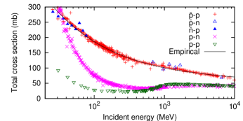
Figure 1: Antinucleon-nucleon ($\bar{N}N$) total cross sections at incident energies from 30 MeV to 10 GeV. Nucleon-nucleon ($NN$) total cross sections are also plotted for comparison. A curve denotes the empirical parametrization of Eq. (7) for the $\bar{N}N$ total cross sections used in this paper.

For describing the $\bar{N}A$ scattering, it is essential to use a reasonable $\Gamma_{\bar{N}N}$ that describes $\bar{N}N$ elementary processes. Here we take a phenomenological approach to determine the $\bar{N}N$ profile function in order to obtain a global description of the $\bar{N}A$ scattering in a wide range of the incident energies from few hundred MeV to GeV. Though it is beyond the scope of this paper, the construction of the $\bar{N}N$ profile function based on the genuine $\bar{N}{N}$ interaction is interesting. We note that the recent work Vorabbi19 reproduced the experimental data of $\bar{p}A$ scattering at about 200 MeV by using the microscopic wave functions and the $t$-matrix derived from the $\bar{N}N$ interaction based on the chiral effective field theory.

Here we take the $\bar{N}N$ profile function as usual finite-range within a Gaussian form Ray79

$$\Gamma_{\bar{N}N}(\bm{b})=\frac{1-i\alpha_{\bar{N}N}}{4\pi\beta_{\bar{N}N}}\sigma_{\bar{N}N}^{\rm tot}\exp\left(-\frac{\bm{b}^{2}}{2\beta_{\bar{N}N}}\right),$$ (6)

where $\sigma_{\bar{N}N}^{\rm tot}$ is the $\bar{N}N$ total cross section, $\alpha_{\bar{N}N}$ is the ratio of the real to imaginary parts of the $\bar{N}N$ scattering amplitude at the zero degree, and $\beta_{\bar{N}N}$ is the slope parameter, which is responsible for describing the $\bar{N}N$ elastic scattering at forward angles. As we will explain it later, these parameters will be fixed to follow the available $\bar{N}N$ and $\bar{N}A$ scattering data for each incident energy, although they are limited.

Figure 1 displays the experimental $\sigma_{\bar{N}N}^{\rm tot}$ as a function of the incident energy PDG . The $NN$ total cross sections, $\sigma_{NN}^{\rm tot}$, are also presented for comparison. As we see in the figure, $\sigma_{\bar{N}N}^{\rm tot}$ is approximately 4 times larger than $\sigma_{NN}^{\rm tot}$ at around 100 MeV, and approximately 3 times at around 1000 MeV. These properties must give the different sensitivity in the $\bar{N}A$ scattering to the nuclear density profile from that in the $NA$ scattering. For a practical use, we parametrize $\sigma_{\bar{N}N}^{\rm tot}$ in unit of mb as a function of the incident energy $E$ in unit of MeV with the same form of Ref. Bertulani10 as

$$\sigma_{\bar{N}N}^{\rm tot}(E) =60.092-361.807/E$$

$$+1301.09/\sqrt{E}-2.5882\times 10^{-4}E$$

$$(30\,{\rm MeV}<E<10\,{\rm GeV}).$$ (7)

As shown in Fig. 1, this empirical parametrization nicely follows the experimental $\bar{N}N$ data from 30 MeV to 10 GeV. Since the experimental data are limited, especially $\bar{p}n$ scattering cross section data PDG , we assume the same value for both $\bar{p}n$ and $\bar{p}p$ cross sections and $\alpha_{\bar{N}N}=0$. Note that within the OLA the reaction probability of Eq. (1), which is the integrand of the total reaction cross section, does not depend on $\alpha_{\bar{N}N}$ as $|e^{i\chi(\bm{b})}|^{2}=e^{-2{\rm Im}\chi(\bm{b})}$. The remaining parameter $\beta_{\bar{N}N}$, which determines the effective range of the interaction, will be fixed in the next subsection.

III.2 Antiproton-nucleus scattering

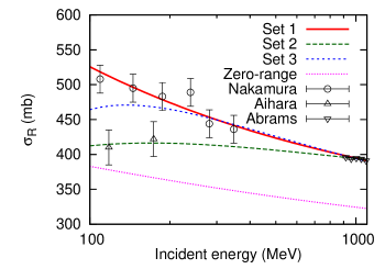
Figure 2: Total reaction cross sections of $\bar{p}$-¹²C scattering as a function of incident energy. The experimental data are taken from Refs. Abrams71 ; Aihara81 ; Nakamura84 . The density distribution of ¹²C is taken as the harmonic-oscillator-type density distribution Ibrahim09 whose width parameter is fixed so as to to reproduce the rms point-proton radius extracted from the electron scattering Angeli13 .

Here we make use of the $\bar{p}$-¹²C total reaction cross section data to fix $\beta_{\bar{N}N}$ in Eq. (6) because the density profile of ¹²C is well known and the elastic scattering differential cross section data are also available. By minimizing the root-mean-square (rms) deviation between the theoretical and experimental $\bar{p}$-¹²C total reaction cross sections at different incident energies, we determine the energy-dependent $\beta_{\bar{N}N}$ parameters. To obtain a better fit for the experimental cross sections, we assume $\beta_{\bar{N}N}$ as it similar to the energy dependence of the total cross sections (7)

$$\beta_{\bar{N}N}(E)=b_{1}+b_{2}/E+b_{3}/\sqrt{E}.$$ (8)

Since the experimental data of the total reaction cross sections are somewhat scattered at around 200 MeV, we test three sets of parameters to give the smallest rms deviation for only with the data of Ref. Nakamura84 (Set 1), of Ref. Aihara81 (Set 2), and including both cross sections at around 200 MeV (Set 3). All the potential sets include the data of Ref. Abrams71 .

Figure 2 plots the calculated total reaction cross sections of the $\bar{p}$-¹²C scattering with Sets 1–3 as a function of the incident energies. The results with Sets 1 and 2 are similar at the incident energies beyond $\approx 200$ MeV, and the ones with Set 3 show quite differently from these Sets below $\approx 800$ MeV. Note that the zero-range profile function ($\beta_{\bar{N}N}=0$) defined explicitly by

$$\Gamma_{\bar{N}N}(\bm{b})=\frac{1-i\alpha_{\bar{N}N}}{2}\sigma_{\bar{N}N}^{\rm tot}\delta(\bm{b})$$ (9)

does not explain the experimental data at all, giving significant underestimation of the data. The resulting parameter sets of Eq. (8) are given in Table 1. In general, larger $\beta_{\bar{N}N}$ values $\approx 0.5$–1.3 fm² are needed to explain the experimental $\bar{p}$-¹²C data, while those of the $NN$ profile functions are ranging from 0.1 to 0.7 fm² Horiuchi07 .

These large $\beta_{\bar{N}N}$ values required in describing the $\bar{N}A$ scattering can be clarified by comparing the slope parameter dependence of the reaction probabilities of Eq. (1) for the $\bar{p}A$ and $pA$ scattering. Figure 3 draws these reaction probabilities as a function of the impact parameter $b$ for different slope parameters at 180 and 1000 MeV, where the experimental total reaction cross sections are available. To compare the role of the slope parameter, we also take the $NN$ profile function with $\alpha_{NN}=0$ and vary $\beta_{NN}$. In the $p$-¹²C scattering, since the $NN$ total cross section is not large enough in such a light nucleus, the reaction probabilities do not reach at unity even at the center of the nucleus ($b=0$), leading to some slope parameter dependence in the whole regions. In contrast, in the $\bar{p}$-¹²C scattering, the probabilities are unity up to around the nuclear radius $\approx 3$ fm. The tail part of the density distribution beyond the nuclear radius crucially contributes to the total reaction cross sections. In fact, the total reaction cross section at 180 MeV increases 366, 430, and 487 mb with $\beta_{\bar{N}N}=0.0,$ 0.4, and 0.8 fm^-2, respectively, whereas for the $N$-¹²C scattering, the enhancement is not as significant as that for the antiproton: 206, 225, and 246 for $\beta_{NN}=0.0$, 0.4, and 0.8 fm^-2, respectively. The reaction probabilities at 1000 MeV behave almost the same as these at 180 MeV with less extended distributions because of smaller $\bar{N}N$ total cross sections compared to these at 180 MeV. Introducing the finite range in the profile function is essential to describe the $\bar{p}A$ total reaction cross sections.

Table 1: Parameters in the parametrization of the slope parameter $\beta_{\bar{N}N}$ of Eq. (8).

		$b_{1}$ (fm2)	$b_{2}$ (fm2MeV)	$b_{3}$ (fm2MeV1/2)
Set 1		0.4202	$-4.516\times 10^{-5}$	4.516
Set 2		0.7402	$5.799\times 10^{-5}$	$-$5.799
Set 3		0.1483	$-$142.1	17.40

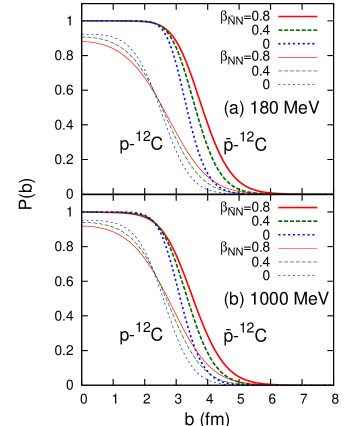
Figure 3: Reaction probabilities of $\bar{p}$- and $p$-¹²C in thick and thin lines, respectively, as a function of impact parameter $b$ with different slope parameters for the profile functions at (a) 180 and (b) 1000 MeV.

At the end of this section, the validity of the profile function is examined by comparing the theoretical elastic scattering differential cross sections to the experimental data for ¹²C, ¹⁶O, and ⁴⁰Ca. Figure 4 shows the elastic scattering differential cross sections for those target nuclei at the incident energy of 180 MeV. We find that Set 1 best reproduces the $\bar{p}A$ elastic scattering differential cross section data up to the second minima. Note that Set 2 also give a good description, in which its slope parameter is accidentally almost the same as these of Set 1 at this incident energy region, resulting in the similar total reaction cross sections shown in Fig. 2. Therefore, we propose the parametrizations of Sets 1 and 2 as a “minimal” profile function to describe the $\bar{p}A$ scattering, and hereafter we use Set 1 otherwise noted. While we see overall agreement of the theoretical cross sections with the experimental data, at a closer look, the cross sections at around the minima are not reproduced well. This can be improved by including higher order terms which are ignored in the OLA (5). See, for example, Fig. 1 (a) of Ref. Hatakeyama19 for $p$-¹²C scattering.

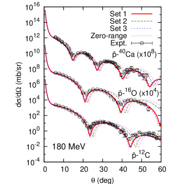
Figure 4: Elastic scattering differential cross sections of $\bar{p}$-¹²C, ¹⁶O, and ⁴⁰Ca scattering at 180 MeV with different choices of the profile function. The experimental data are taken from Ref. Garreta84 ; Bruge86 . The cross sections are multiplied by $10^{4}$ and $10^{8}$ for those for ¹⁶O, and ⁴⁰Ca, respectively. The harmonic-oscillator-type densities Ibrahim09 consistent with the experimental charge radii Angeli13 are used.

IV Discussions

We have confirmed that the $\bar{p}A$ reactions are fairly well reproduced by the present reaction model. Here we discuss what density regions are actually probed by the antiproton. To quantify this, we display the reaction probabilities of Eq. (1) as a function of the densities in place of $b$.

Figure 5 plots the reaction probabilities of the $\bar{p}A$ and $pA$ scattering for ¹²C and ⁴⁰Ca at 180 MeV as a function of the values of $\rho_{m}/\rho_{0}$, which is the fraction of the matter density distributions ($\rho_{m}=\rho_{n}+\rho_{p}$) to the density at the origin or the central nuclear density ($\rho_{0}$). FOr ⁴⁰Ca, at the high density or internal regions, the probabilities are unity showing the complete absorption and drop at certain density regions depending on the incident particles. For the antiproton scattering, the plateau extends being still unity even at the radius that the central density is halved $\rho_{m}/\rho_{0}$=0.5, and reaches beyond $\rho_{m}/\rho_{0}\lesssim 10^{-4}$, which is two order of magnitude smaller than that of the proton scattering. When the probability becomes 0.5, which corresponds to 5.5 fm of the radius of a sphere, $\rho_{m}/\rho_{0}$ becomes 0.02. This value is one order of magnitude smaller than that of the proton scattering, $\rho_{m}/\rho_{0}=0.2$, corresponding 4.2 fm of the radius of a sphere. This confirms that the antiproton can probe the variation of the density distribution at around $\sim 1/100$ of the central density and could be sensitive to the region of $\rho_{m}/\rho_{0}\sim 10^{-4}$. This density region corresponds to the tail of a typical two-neutron halo nucleus $\rho_{m}/\rho_{0}\lesssim 10^{-2}$ Horiuchi06 .

The similar behavior is also found in a case of ¹²C. The plateau also appears for the $\bar{p}$-¹²C, while the reaction probability does not reach unity for the $p$-¹²C scattering. Because the ¹²C consists mostly by the nuclear surface, the optical depth is not small enough.

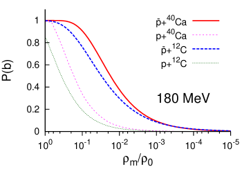
Figure 5: Reaction probabilities of ¹²C and ⁴⁰Ca as a function of the fraction of the nuclear density to the central density. See text for details.

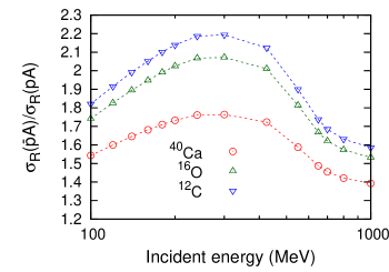
Figure 6: Ratio of total reaction cross sections of ¹²C, ¹⁶O, and ⁴⁰Ca for antiproton and proton scattering as a function of the incident energy.

In order to compare the different sensitivity in the $\bar{p}A$ and $pA$ scattering, we introduce the ratio of the total reaction cross sections of the $\bar{p}A$ and $pA$ scattering, $\sigma_{R}(\bar{p}A)/\sigma_{R}(pA)$. The parameter sets of the profile function of Ref. Ibrahim08 are used to calculate $\sigma_{R}(pA)$. Let us first discuss a medium-heavy nucleus by taking ⁴⁰Ca as an example, where the separation of the bulk and the surface part is developing Kohama05 . The curve is shown in Fig. 6. Reflecting the above fact, the antiproton interacts with less nucleons than the whole numbers of this nucleus, because the reaction probability saturate at the thick density region, i.e., the bulk region, as can be seen in Fig. 5. The antiproton interacts only with the nucleons in the nuclear surface. This is the reason why the ratio does not become large despite the fact that the $\bar{N}N$ cross section is 3–4 times larger than the $NN$ one. What will happen for the case of light nuclei, such as ¹²C, and ¹⁶O, where the nuclear surface is a whole body Kohama05 . Since the most of the composite nucleons are sitting in the surface region, the incident antiproton can interact with those nucleons, which drastically increases the total reaction cross sections of the antiproton than that of ⁴⁰Ca as one can see from Fig. 6. The energy dependence of the ratio can easily understood by looking at the values of the elementary cross sections shown in Fig. 2. For example, the $NN$ total cross sections are minimum at this energy region while the $\bar{N}N$ ones decreases monotonically, leading to the peak of the ratio at around 300 MeV.

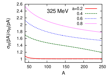
Figure 7: Ratio of total reaction cross sections for antiproton and proton scattering at 325 MeV calculated using the 2pF density distributions with various diffuseness parameters as a function of the mass number $A$. See text for details.

To extend the above discussion more general, we employ two-parameter Fermi (2pF) distributions as a nuclear matter density

$$\rho_{N}(r)=\frac{\rho_{0}}{1+\exp\left(\frac{r-R}{a}\right)}.$$ (10)

For a given diffuseness parameter $a$, $\rho_{0}$ and $R$ are determined by the normalization to the mass number $A$ and the rms matter radius being followed as $\sqrt{\frac{3}{5}}1.2\times A^{1/3}$ Hatakeyama18 . By varying the diffuseness parameter, we discuss the role of the surface density profiles for medium to heavy nuclei. Figure 7 plots the calculated cross section ratios with various diffuseness parameters at 325 MeV, where the ratio is maximized. Here the averaged $NN$ profile function Horiuchi07 is used to calculate the $NA$ total reaction cross sections. For a small diffuseness parameter, for example, $a=0.2$ fm, the ratio is almost unity. Because the reaction probabilities in the internal regions are already saturated and a few nucleon exists at around the nuclear surface, there is no space to increase the total reaction cross sections even with the larger total $\bar{N}N$ cross sections. As expected, the smaller diffuseness, the smaller ratio becomes. We find that the ratio strongly depends on the diffuseness parameter sufficient to determine the nuclear surface “diffuseness” by measuring both the total reaction cross sections for the $\bar{p}A$ and $pA$ scattering at the same incident energy. We note that the typical diffuseness parameters are around 0.45–0.55 fm, and possibly $\gtrsim 0.6$ fm for well-deformed and weakly bound nuclei Hatakeyama18 ; Horiuchi17 . The ratio decreases with increasing the mass number because the nuclear surface contribution becomes relatively smaller than the bulk contribution.

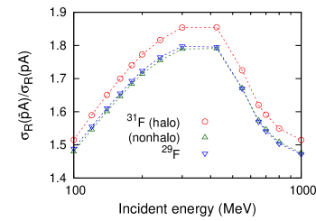
Figure 8: Same as Fig. 6 but of ^29,31F. The halo and nonhalo density profiles for ³¹F are employed. See text for details.

Finally, we investigate the different sensitivity to a dilute nuclear density profile beyond the nuclear half density radius. Though the antiproton scattering on unstable nuclei is still not feasible at present, we take an example of a possible two-neutron halo nucleus ³¹F Michel20 ; Masui20 , which is located at the fluorine dripline Ahn19 . The halo formation depends on the shell gap between and $0f_{7/2}$ and $1p_{3/2}$ orbits. The inverted configuration, that is, the dominance of the latter orbit forms the halo structure. We use these density distributions of ³¹F with the $(1p_{3/2})^{2}$ (halo) and $(0f_{7/2})^{2}$ (nonhalo) dominance, which correspond to the cases A and B in Ref. Masui20 , and calculate $\sigma_{R}(\bar{p}A)/\sigma_{R}(pA)$ to see the sensitivity to the halo tail. Figure 8 plots the ratios of ³¹F as a function of the incident energy. For the sake of comparison, the ones of ²⁹F are also calculated with the harmonic-oscillator type density distribution Masui20 . The ³¹F with the halo tail gives the largest ratios, while the nonhalo density profile produces the almost the same behavior of that of ²⁹F, exhibiting the standard ratio as expected from Fig. 6. This fact clearly shows that the advantage of the $\bar{p}A$ scattering for the dilute density distribution further than the nuclear surface.

Since the antiproton has different sensitivity to the nuclear density profile, one can scan the density distribution by measuring the elastic scattering differential cross sections using different probes, the antiproton and proton. As expected from the diffraction model Bethe and the recent Glauber model analysis Hatakeyama18 , when one performs the antiproton elastic scattering measurement, elastically scattered particles come to the forward angles more concentrated than in the proton case, which makes the measurement easier. A detailed study along this direction will give more precise determination of the nuclear density distributions beyond the nuclear half density radius.

As will be shown in Appendix A, we additionally remark that the black-sphere empirical relation, Eq. (11), is found out to be valid within $\approx 10$% for this antiproton case. This will support that the same line of the discussion in Ref. Hatakeyama18 but for antiproton can be extended here.

V Conclusions

We have investigated the feasibility of using the antiproton-nucleus ($\bar{p}A$) scattering as a probe of the nuclear surface density distribution. We have shown that the high-energy $\bar{p}A$ reactions are well described with the Glauber model with a “minimal” profile function, which reproduces the $\bar{p}$-¹²C total reaction cross sections in a wide range of the incident energies, through a comparison to the available experimental data of the antiproton elastic scattering differential cross sections on ¹²C, ¹⁶O, and ⁴⁰Ca.

We have quantified what density regions are sensitive to the $\bar{p}A$ scattering by comparing the reaction probabilities obtained for the $\bar{p}A$ and $pA$ scattering. In the $pA$ scattering, the reaction probability becomes half at the radius of a sphere that corresponds to $\approx 1/10$ of the central density, whereas in the $\bar{p}A$ scattering the reaction probability is halved at the tail region of the nuclear density distribution, $\approx 1/100$ of the central density. The reaction probability beyond the nuclear half density radius is significantly increased even at the low density due to much larger elementary cross sections than the $NN$ ones. This results in the large enhancement of the total reaction cross sections, especially for light nuclei which consist mostly by the nuclear surface. We have shown that the enhancement of the cross section is significant enough to determine the density profile around the nuclear surface, the nuclear “diffuseness”. To explore the outer part of the density distribution of the exotic nuclei, the sensitivity to the dilute nuclear tail has also been quantified by taking an example of ³¹F, which is a candidate of a two-neutron halo nucleus Michel20 ; Masui20 .

The antiproton probes the dilute density distributions around and beyond the nuclear surface more efficiently than the proton. Measuring the both $\bar{p}A$ and $pA$ total reaction and elastic scattering cross sections could offer the opportunity to precisely determine the nuclear surface density profile including the dilute nuclear tail. Experimental search for new halo candidates will extend for heavier nuclei beyond ^29,31F. Recently, unexpectedly rapid increase of the nuclear radii of neutron-rich calcium isotopes towards larger neutron excess was reported Tanaka20 . A possible interpretation could be a drastic change of the structure of the core nucleus and is related to the properties of the valence single particle orbits Horiuchi20 , which determine the nuclear diffuseness. Though no experimental facility might exist so far doing the measurement of the high-energy antiproton off an unstable nucleus, if realized, as the electron scattering did scrit2017 , the antiproton can be one of the best probes to unveil the exotic structure of neutron-rich nuclei.

Appendix A Black sphere picture in antiproton-nucleus scattering

The antiproton scattering offers more absorptive scattering process than that of the proton scattering. One may think that the black sphere (BS) model Kohama04 ; Kohama05 ; BS3 ; Kohama16 is expected to work better than that of the $NA$ scattering. For this purpose, we evaluate the BS estimate where the total reaction cross section is calculated by the first peak position of the diffraction peak: Assuming that a nucleus is completely absorptive within a sharp-cut nuclear radius $a_{\rm BS}$, the total reaction cross section

$$\sigma_{\rm BS}=\pi a_{\rm BS}^{2}$$ (11)

can be related to the BS radius Kohama04

$$a_{\rm BS}=\frac{5.1356\cdots}{2p\sin(\theta_{M}/2)},$$ (12)

where $p$ $(=K)$ is the momentum between the two colliding particles. If the $\bar{N}A$ scattering is ideally described with the BS model, a slope of the BS cross sections must follow the $y=x$ line in this correlation plot.

Figure 9 plots $\sigma_{BS}$ against $\sigma_{R}$ with the 2pF density distributions of Eq. (10). The $\sigma_{BS}$ deviates from $\sigma_{R}$ with increasing the diffuseness parameter of the density distribution. We note that the Glauber calculation with the zero-range profile function is nothing but the complete absorption or the BS model if the elementary cross section is large enough. Actually, as displayed in Fig. 9, the correlation plot follows the $y=x$ line with a sharp-cut square-well ($a=0$) using the zero-range profile function. The deviation comes from the two facts in reality, that are, the nuclear surface diffuseness and the finiteness of the interaction. Though the black sphere model explains most of the bulk properties of the $\bar{p}A$ scattering, the differences are typically $\approx 10$% in $A=40$–250 with $a=0.4$–0.6 fm for all the incident energies, which are a bit larger than the case of the $pA$ scattering Hatakeyama18 due to higher sensitivity to the nuclear surface.

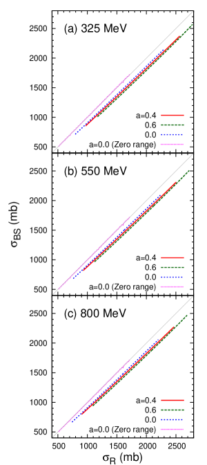
Figure 9: Correlation plot of $\sigma_{BS}$ versus $\sigma_{R}$ at (a) 325, (b) 550, and (c) 800 MeV for the antiproton scattering. Thin lines in gray denote a $y=x$ line for a guide of eyes.

References

- (1) I. Tanihata, H. Hamagaki, O. Hashimoto, Y. Shida, N. Yoshikawa, K. Sugimoto, O. Yamakawa, T. Kobayashi, and N. Takahashi, Phys. Rev. Lett. 55, 2676 (1985).
- (2) I. Tanihata, H. Savajols, and R. Kanungo, Prog. Part. Nucl. Phys. 68, 215 (2013), and references therein.
- (3) S. Bagchi, R. Kanungo, Y. K. Tanaka, H. Geissel, P. Doornenbal, W. Horiuchi, G. Hagen, T. Suzuki, N. Tsunoda, D. Ahn et al., Phys. Rev. Lett. 124, 222504 (2020).
- (4) N. Michel, J. G. Li, F. R. Xu, and W. Zuo, Phys. Rev. C 101, 031301(R) (2020).
- (5) H. Masui, W. Horiuchi, and M. Kimura, Phys. Rev. C 101, 041303(R) (2020).
- (6) J. Singh, J. Casal, W. Horiuchi, L. Fortunato, and A. Vitturi, Phys. Rev. C 101, 024310 (2020).
- (7) L. Fortunato, J. Casal, W. Horiuchi, J. Singh, and A. Vitturi, Commun. Phys. 3, 132 (2020).
- (8) H. de Vries, C. W. de Jager, and C. de Vries, Atomic Data and Nuclear Data Tables 36, 495 (1987).
- (9) S. Terashima, H. Sakaguchi, H. Takeda, T. Ishikawa, M. Itoh, T. Kawabata, T. Murakami, M. Uchida, Y. Yasuda, M. Yosoi et al., Phys. Rev. C 77, 024317 (2008).
- (10) J. Zenihiro, H. Sakaguchi, T. Murakami, M. Yosoi, Y. Yasuda, S. Terashima, Y. Iwao, H. Takeda, M. Itoh, H. P. Yoshida, and M. Uchida, Phys. Rev. C 82, 044611 (2010).
- (11) H. Sakaguchi and J. Zenihiro, Prog. Part. Nucl. Phys. 97, 1 (2017), and references therein.
- (12) M. Tanabashi, K. Hagiwara, K. Hikasa, K. Nakamura, Y. Sumino, F. Takahashi, J. Tanaka, K. Agashe, G. Aielli, C. Amsler et al. (Particle Data Group), Phys. Rev. D 98, 030001 (2018), and 2019 update.
- (13) W. Horiuchi, Y. Suzuki, and T. Inakura, Phys. Rev. C 89, 011601(R) (2014).
- (14) W. Horiuchi, S. Hatakeyama, S. Ebata, and Y. Suzuki, Phys. Rev. C 93, 044611 (2016).
- (15) S. Hatakeyama, W. Horiuchi, and A. Kohama, Phys. Rev. C 97, 054607 (2018).
- (16) A. Obertelli et al. (PUMA collaboration), PUMA: Antiprotons and radioactive nuclei, Technical Report No. CERN-INTC-2018-023, INTC-M-018 (CERN, Geneva, 2018).
- (17) A. Obertelli et al. (PUMA collaboration), PUMA: Antiprotons and radioactive nuclei, Technical Report No. CERN-SPSC-2019-033, SPSC-P-361 (CERN, Geneva, 2019).
- (18) J. Lichtenstadt, A. I. Yavin, S. Janouin, P. Birien, G. Bruge, A. Chaumeaux, D. Drake, D. Garreta, D. Legrand, M. C. Lemaire et al., Phys. Rev. C 32, 1096 (1985).
- (19) A. Kohama, K. Iida, and K. Oyamatsu, J. Phys. Soc. Jpn. 85, 094201 (2016).
- (20) E. Friedman and J. Lichtenstadt, Nucl. Phys. A 455, 573 (1986).
- (21) R. J. Glauber, Lectures in Theoretical Physics, edited by W. E. Brittin and L. G. Dunham (Interscience, New York, 1959), Vol. 1, p.315.
- (22) Y. Suzuki, R. G. Lovas, K. Yabana, and K. Varga, Structure and reactions of light exotic nuclei (Taylor & Francis, London, 2003).
- (23) K. Varga, S. C. Pieper, Y. Suzuki, and R. B. Wiringa, Phys. Rev. C 66, 034611 (2002).
- (24) T. Nagahisa and W. Horiuchi, Phys. Rev. C 97, 054614 (2018).
- (25) R. H. Bassel and C. Wilkin, Phys. Rev. 174, 1179 (1968).
- (26) B. Abu-Ibrahim, S. Iwasaki, W. Horiuchi, A. Kohama, and Y. Suzuki, J. Phys. Soc. Jpn., Vol. 78, 044201 (2009).
- (27) S. Hatakeyama, S. Ebata, W. Horiuchi, and M. Kimura, J. Phys.: Conf. Ser. 569, 012050 (2014).
- (28) S. Hatakeyama, S. Ebata, W. Horiuchi, and M. Kimura, JPS Conf. Proc., Vol. 6, 030096 (2015).
- (29) W. Horiuchi, Y. Suzuki, B. Abu-Ibrahim, and A. Kohama, Phys. Rev. C 75, 044607 (2007).
- (30) B. Abu-Ibrahim, W. Horiuchi, A. Kohama, and Y. Suzuki, Phys. Rev. C 77, 034607 (2008); ibid 80, 029903(E) (2009); 81, 019901(E) (2010).
- (31) M. Vorabbi, M. Gennari, P. Finelli, C. Giusti, and P. Navrátil, Phys. Rev. Lett. 124, 162501 (2020).
- (32) L. Ray, Phys. Rev. C 20, 1857 (1979).
- (33) C. A. Bertulani and C. De Conti, Phys. Rev. C 81, 064603 (2010).
- (34) I. Angeli, K. P. Marinova, At. Data Nucl. Tables 99, 69 (2013).
- (35) K. Nakamura, J. Chiba, T. Fujii, H. Iwasaki, T. Kageyama, S. Kuribayashi, T. Sumiyoshi, T. Takeda, H. Ikeda, and Y. Takada, Phys. Rev. Lett. 52, 731 (1984).
- (36) H. Aihara, J. Chiba, H. Fujii, T. Fujii, H. Iwasaki, T. Kamae, K. Nakamura, T. Sumiyoshi, Y. Takada, T. Takeda, M. Yamauchi, and H. Fukuma, Nucl. Phys. A 360, 291 (1981).
- (37) R. J. Abrams, R. L. Cool, G. Giacomelli, T. F. Kycia, B. A. Leontic K. K. Li, A. Lundby, D. N. Michael, and J. Teiger, Phys. Rev. D 4, 3235 (1971).
- (38) D. Garreta, P. Birien, G. Bruge, A. Chaumeaux, D. Drake, S. Janouin, D. Legrand, M. Lemaire, B. Mayer, J. Pain et al., Phys. Lett. B 149, 64 (1984).
- (39) G. Bruge, A. Chaumeaux, P. Birien, D. Drake, D. Garreta, S. Janouin, D. Legrand, M. Lemaire, B. Mayer, J. Pain et al., Phys. Lett. B 169, 14 (1986).
- (40) S. Hatakeyama and W. Horiuchi, Nucl. Phys. A 985, 20 (2019).
- (41) W. Horiuchi and Y. Suzuki, Phys. Rev. C 74, 034311 (2006).
- (42) A. Kohama, K. Iida, and K. Oyamatsu, Phys. Rev. C 72, 024602 (2005).
- (43) W. Horiuchi, S. Ebata, and K. Iida, Phys. Rev. C 96, 035804 (2017).
- (44) D. S. Ahn, N. Fukuda, H. Geissel, N. Inabe, N. Iwasa, T. Kubo, K. Kusaka, D. J. Morrissey, D. Mukai, T. Nakamura et al., Phys. Rev. Lett. 123, 212501 (2019).
- (45) G. Placzek and H. A. Bethe, Phys. Rev. 57, 1075 (1940).
- (46) M. Tanaka, M. Takechi, M. Fukuda, D. Nishimura, T. Suzuki, Y. Tanaka, T. Moriguchi, D. S. Ahn, A. Aimaganbetov, M. Amano et al., Phys. Rev. Lett. 124, 102501 (2020).
- (47) W. Horiuchi and T. Inakura, Phyr. Rev. C 101, 061301(R) (2020).
- (48) K. Tsukada, A. Enokizono, T. Ohnishi, K. Adachi, T. Fujita, M. Hara, M. Hori, T. Hori, S. Ichikawa, K. Kurita et al., Phys. Rev. Lett. 118, 262501 (2017).
- (49) A. Kohama, K. Iida, and K. Oyamatsu, Phys. Rev. C 69, 064316 (2004).
- (50) K. Iida, A. Kohama, and K. Oyamatsu, J. Phys. Soc. Japan 76, 044201 (2007).