Eigenvalues of tridiagonal Hermitian Toeplitz matrices
with perturbations in the off-diagonal corners

Abstract

In this paper we study the eigenvalues of Hermitian Toeplitz matrices with the entries $2,-1,0,\ldots,0,-\alpha$ in the first column. Notice that the generating symbol depends on the order $n$ of the matrix. If $|\alpha|\leq 1$, then the eigenvalues belong to $[0,4]$ and are asymptotically distributed as the function $g(x)=4\sin^{2}(x/2)$ on $[0,\pi]$. The situation changes drastically when $|\alpha|>1$ and $n$ tends to infinity. Then the two extreme eigenvalues (the minimal and the maximal one) lay out of $[0,4]$ and converge rapidly to certain limits determined by the value of $\alpha$, whilst all others belong to $[0,4]$ and are asymptotically distributed as $g$. In all cases, we transform the characteristic equation to a form convenient to solve by numerical methods, and derive asymptotic formulas for the eigenvalues.

Keywords: eigenvalue, tridiagonal matrix, Toeplitz matrix, perturbation, asymptotic expansion.

MSC (2010): 15B05, 15A18, 41A60, 65F15, 47A55.

1 Introduction

Toeplitz matrices appear naturally in the study of shift-invariant models with zero boundary conditions. The general theory of such matrices is explained in the books and reviews [6, 7, 8, 11, 14, 15]. Efficient formulas for the determinants of banded symmetric Toeplitz matrices were found in [20, 12]. The determinants, minors, cofactors, and eigenvectors of banded Toeplitz matrices were recently expressed in terms of skew Schur polynomials, see [1, 17]. The individual behavior of the eigenvalues of Hermitean Toeplitz matrices was investigated in [2, 3, 4, 5, 10].

Determinants of non-singular Toeplitz matrices with low-rank perturbations were studied in [6]. The eigenvalues and eigenvectors of tridiagonal Toeplitz matrices with some special perturbations on the diagonal corners are computed in [9, Section 1.1] and [18]. The determinants and inverses of a family of non-symmetric tridiagonal Toeplitz matrices with perturbed corners are computed in [22].

Yueh and Cheng [24] considered the tridiagonal Toeplitz matrices with four perturbed corners. Using the techniques of finite differences they derived the characteristic equation in a trigonometric form and formulas for the eigenvectors, in terms of the eigenvalues. For some special values of the parameters, they computed explicitly the eigenvalues. Unlike the present paper, [24] deals with arbitrary complex coefficients and does not contain the analysis of the localization of the eigenvalues nor approximate formulas for the eigenvalues.

In this paper we study the spectral behavior of one family of Hermitean tridiagonal Toeplitz matrices with perturbations at the entries $(n,1)$ and $(1,n)$, where $n$ is the order of the matrix. For every $\alpha$ in $\mathbb{C}$ and every natural number $n\geq 3$ we denote by $A_{\alpha,n}$ the $n\times n$ Toeplitz matrix generated by the following function which depends on the parameters $\alpha$ and $n$:

$$-\overline{\alpha}t^{-n+1}-t^{-1}+2-t-\alpha t^{n-1}.$$ (1)

After the change of variable $t=\exp(ix)$, the generating symbol results in

$$h_{\alpha,n}(x)=4\sin^{2}(x/2)-2\operatorname{Re}(\alpha\,e^{i(n-1)x}).$$

For example, if $n=6$,

$$A_{\alpha,6}=\begin{bmatrix}[r]2&-1&0&0&0&-\overline{\alpha}\\ -1&2&-1&0&0&0\\ 0&-1&2&-1&0&0\\ 0&0&-1&2&-1&0\\ 0&0&0&-1&2&-1\\ -\alpha&0&0&0&-1&2\end{bmatrix}.$$

Such matrices may appear in the study of one-dimensional shift-invariant models on a finite interval, with some special interactions between the extremes of the interval.

For $\alpha=0$, the matrix $A_{\alpha,n}$ is the well studied tridiagonal Toeplitz matrix with the symbol $g\coloneqq h_{0,n}$, i.e.

$$g(x)\coloneqq 4\sin^{2}(x/2).$$ (2)

The characteristic polynomial of $A_{0,n}$ is $\det(\lambda I_{n}-A_{0,n})=U_{n}((\lambda-2)/2)$, where $U_{n}$ is the $n$th Chebyshev polynomial of the second type, and the eigenvalues of $A_{0,n}$ are $g(j\pi/(n+1))$, $1\leq j\leq n$. For general $\alpha$, the characteristic polynomial of $A_{\alpha,n}$ can be expressed in terms of $U_{n}$ and $U_{n-2}$. We are able to compute the eigenvalues of $A_{\alpha,n}$ explicitly only for $|\alpha|=1$ or $\alpha=0$. For $|\alpha|\neq 1$, applying an appropriate trigonometric or hyperbolic change of variable, we describe the localization of the eigenvalues, transform the characteristic equation to a form that can be solved by the fixed point iteration, and get asymptotic formulas.

It turns out that the cases $|\alpha|<1$ (“weak perturbations”) and $|\alpha|>1$ (“strong perturbations”) are essentially different: if $|\alpha|>1$, then the extreme eigenvalues go outside the interval $[0,4]$ and need a special treatment. Below we present the corresponding results separately, starting with the simpler case $|\alpha|<1$. In Sections 3 and 5 we give the corresponding proofs. The case $|\alpha|=1$ can be viewed as a limit of the case $|\alpha|<1$, but the results in this case are much simpler, see Section 4. Finally, in Section 6 we discuss some numerical tests.

2 Main results

The matrices $A_{\alpha,n}$ are Hermitean, their eigenvalues are real, and we enumerate them in the ascending order:

$$\lambda_{\alpha,n,1}\leq\lambda_{\alpha,n,2}\leq\cdots\leq\lambda_{\alpha,n,n}.$$

2.1 Main results for weak perturbations

Recall that the function $g$ is defined by (2). It strictly increases on $[0,\pi]$ taking values from $0$ to $4$.

Theorem 1 (localization of the eigenvalues for weak perturbations).

Let $\alpha\in\mathbb{C}$, $|\alpha|\leq 1$, $\alpha\notin\{-1,1\}$, and $n\geq 3$. Then the matrix $A_{\alpha,n}$ has $n$ different eigenvalues belonging to $(0,4)$. More precisely, for every $j$ in $\{1,\ldots,n\}$,

$$g\left(\frac{(j-1)\pi}{n}\right)<\lambda_{\alpha,n,j}<g\left(\frac{j\pi}{n}\right).$$ (3)

The minimal value of the generating function $h_{\alpha,n}$, for $|\alpha|\leq 1$, may be strictly negative. So, even the inequality $\lambda_{\alpha,n,1}>0$, which is a very small part of Theorem 1, is not obvious.

Theorem 1 implies that the eigenvalues of $A_{\alpha,n}$, as $n$ tends to $\infty$, are asymptotically distributed as the values of the function $g$. This follows also from the theory of locally Toeplitz sequences [21, 19, 13] or, more specifically, from Cauchy interlacing theorem, since the matrices $A_{\alpha,n}$ are obtained from the tridiagonal Toeplitz matrices $A_{0,n}$ by low-rank perturbations.

Our next goal is to transform the characteristic equation into a convenient form. For every $\alpha$ in $\mathbb{C}$ with $\alpha\notin\{-1,1\}$ and every integer $j$ we define the function $\eta_{\alpha,j}\colon[0,\pi]\to\mathbb{R}$ by

$$\eta_{\alpha,j}(x)\coloneqq-2\arctan\left(\left((-1)^{j+1}k_{\alpha}\cot{(x)}+\sqrt{k_{\alpha}^{2}\cot^{2}{(x)}+l_{\alpha}^{2}}\right)^{(-1)^{j}}\right),$$ (4)

where

$$k_{\alpha}\coloneqq\frac{1-|\alpha|^{2}}{|1+\alpha|^{2}},\qquad l_{\alpha}\coloneqq\frac{|1-\alpha|}{|1+\alpha|}.$$ (5)

In fact, $\eta_{\alpha,j}$ depends only on $\alpha$ and on the parity of $j$. Thus, for every $\alpha$ there are only two different functions: $\eta_{\alpha,1}$ and $\eta_{\alpha,2}$. These functions take values in $[-\pi,0]$. See a couple of examples on Figure 1.

Figure 1: Functions (4) for $\alpha=0.7+0.6i$ (left) and $\alpha=2+i$ (right).

Motivated by (3), we use the function $g$ as a change of variable in the characteristic equation and put $\vartheta_{\alpha,n,j}\coloneqq g^{-1}(\lambda_{\alpha,n,j})$. Inequality (3) is equivalent to

$$\frac{(j-1)\pi}{n}<\vartheta_{\alpha,n,j}<\frac{j\pi}{n}.$$ (6)

Theorem 2 (characteristic equation for weak perturbations).

Let $\alpha\in\mathbb{C}$, $|\alpha|\leq 1$, $\alpha\notin\{-1,1\}$, $n\geq 3$, and $1\leq j\leq n$. Then the number $\vartheta_{\alpha,n,j}$ satisfies

$$\vartheta_{\alpha,n,j}=\frac{j\pi+\eta_{\alpha,j}(\vartheta_{\alpha,n,j})}{n}.$$ (7)

In Section 3 we show that for $n>N_{1}(\alpha)$, where

$$N_{1}(\alpha)\coloneqq\frac{4(|\alpha|+1)}{||\alpha|-1|},$$ (8)

and for $1\leq j\leq n$, the function in the right-hand side of (7) is contractive. Hence, equation (7) can be solved by the fixed point iteration. Furthermore, we use (7) to derive asymptotic formulas for the eigenvalues.

For $|\alpha|\leq 1$ and $1\leq j\leq n$, define $\lambda^{\operatorname{asympt}}_{\alpha,n,j}$ by

$$\lambda^{\operatorname{asympt}}_{\alpha,n,j} \coloneqq g\left(\frac{j\pi}{n}\right)+\frac{g^{\prime}\left(\frac{j\pi}{n}\right)\eta_{\alpha,j}\left(\frac{j\pi}{n}\right)}{n}$$ (9)

$$\quad+\frac{g^{\prime}\left(\frac{j\pi}{n}\right)\eta_{\alpha,j}\left(\frac{j\pi}{n}\right)\eta_{\alpha,j}^{\prime}\left(\frac{j\pi}{n}\right)+\frac{1}{2}g^{\prime\prime}\left(\frac{j\pi}{n}\right)\eta_{\alpha,j}\left(\frac{j\pi}{n}\right)^{2}}{n^{2}}.$$

Theorem 3 (asymptotic expansion of the eigenvalues for weak perturbations).

Let $\alpha\in\mathbb{C}$, $|\alpha|\leq 1$. Then there exists $C_{1}(\alpha)>0$ such that for $n$ large enough and $1\leq j\leq n$,

$$|\lambda_{\alpha,n,j}-\lambda^{\operatorname{asympt}}_{\alpha,n,j}|\leq\frac{C_{1}(\alpha)}{n^{3}}.$$ (10)

In other words, Theorem 3 claims that $\lambda_{\alpha,n,j}=\lambda^{\operatorname{asympt}}_{\alpha,n,j}+O_{\alpha}\left(\frac{1}{n^{3}}\right)$, where the constant in the upper estimate of the residue term depends on $\alpha$. For simplicity, we state and justify only this asymptotic formula with three exact terms, but there are similar formulas with more terms.

Since the eigenvectors were found in [24] for a more general matrix family, we give the corresponding formulas in Propositions 9 and 18 without proofs.

2.2 Main results for strong perturbations

For the sake of simplicity, we decided to state the following theorems only for large values of $n$. As a sufficient condition, we require $n>N_{2}(\alpha)$, where

$$N_{2}(\alpha)\coloneqq\frac{20\log(|\alpha|+1)-4\log(\log(|\alpha|))}{\log|\alpha|}.$$ (11)

Theorem 4 (localization of the eigenvalues for strong perturbations).

Let $\alpha\in\mathbb{C}$, $|\alpha|>1$, and $n\geq N_{2}(\alpha)$. Then

$$\lambda_{\alpha,n,1}<0,\qquad\lambda_{\alpha,n,n}>4,$$

whereas for $2\leq j\leq n-1$ the eigenvalues $\lambda_{\alpha,n,j}$ belong to $(0,4)$ and satisfy (3).

For some $\alpha$ with $|\alpha|>1$ and for small values of $n$, the eigenvalues $\lambda_{\alpha,n,1}$ and $\lambda_{\alpha,n,n}$ can belong to $[0,4]$. So, the condition $n>N_{2}(\alpha)$ in Theorem 4 cannot be omitted.

In order to solve the characteristic equation for $\lambda<0$ and $\lambda>4$, we use the following changes of variables, respectively:

$$g_{-}(x)\coloneqq-4\sinh^{2}(x/2),\qquad g_{+}(x)\coloneqq 4+4\sinh^{2}(x/2)\qquad(x>0).$$ (12)

Theorem 5 (characteristic equations for strong perturbations).

Let $\alpha\in\mathbb{C}$, $|\alpha|>1$, and $n\geq N_{2}(\alpha)$. Then

$$\lambda_{\alpha,n,1}=g_{-}(\vartheta_{\alpha,n,1}),\qquad\lambda_{\alpha,n,n}=g_{+}(\vartheta_{\alpha,n,n}),$$

where $\vartheta_{\alpha,n,1}$ is the unique positive solution of the equation

$$x=\operatorname{arctanh}\frac{2(|\alpha|^{2}-1)\tanh\frac{nx}{2}}{|\alpha+1|^{2}\tanh^{2}\frac{nx}{2}+|\alpha-1|^{2}},$$ (13)

and $\vartheta_{\alpha,n,n}$ is the unique positive solution of the equation

$$x=\operatorname{arctanh}\frac{2(|\alpha|^{2}-1)\tanh\frac{nx}{2}}{|\alpha+(-1)^{n}|^{2}\tanh^{2}\frac{nx}{2}+|\alpha-(-1)^{n}|^{2}}.$$ (14)

For $2\leq j\leq n-1$, the eigenvalues $\lambda_{\alpha,n,j}$ can be found as in Theorem 2.

Moreover, in Section 5 we prove that the right-hand sides of (13) and (14) are contractive functions on the segment

$$S_{\alpha}\coloneqq\left[\frac{\log|\alpha|}{2},\frac{3\log|\alpha|}{2}\right].$$ (15)

Figure 2 shows an example. In this figure, we glued together three changes of variables ($g_{-}$, $g$, and $g_{+}$) into one spline, using appropriate shifts or reflections.

Figure 2: The points $\vartheta_{\alpha,n,j}$ and the corresponding values of $\lambda_{\alpha,n,j}$ for $\alpha=2+i$, $n=6$. Different scales are used for the axis.

There is another way to see the changes of variables (12): after extending $g$ to an entire function, $g_{-}(x)=g(ix)$ and $g_{+}(x)=g(\pi+ix)$. So, the eigenvalues are obtained by evaluating the function $g$ at some points belonging to a piecewise linear path on the complex plane, see Figure 3.

Figure 3: Points on the complex plane that yield the eigenvalues $\lambda_{\alpha,n,j}$ after applying the function $g$. In this example, $\alpha=2+i$ and $n=6$.

In order to describe the asymptotic behavior of the extreme eigenvalues $\lambda_{\alpha,n,1}$ and $\lambda_{\alpha,n,n}$, we introduce the following notation:

$$s_{\alpha}\coloneqq|\alpha|-2+\frac{1}{|\alpha|},\quad\text{i.e.}\quad s_{\alpha}=\frac{(|\alpha|-1)^{2}}{|\alpha|}=\left(\sqrt{|\alpha|}-\frac{1}{\sqrt{|\alpha|}}\right)^{2}.$$ (16)

Theorem 6 (asymptotic expansion of the eigenvalues for strong perturbations).

Let $\alpha\in\mathbb{C}$, $|\alpha|>1$. As $n$ tends to infinity, the extreme eigenvalues of $A_{\alpha,n}$ converge exponentially to $-s_{\alpha}$ and $4+s_{\alpha}$, respectively:

$$|\lambda_{\alpha,n,1}+s_{\alpha}| \leq\frac{C_{2}(\alpha)}{|\alpha|^{n}},$$ (17)

$$|\lambda_{\alpha,n,n}-4-s_{\alpha}| \leq\frac{C_{2}(\alpha)}{|\alpha|^{n}}.$$ (18)

Here $C_{2}(\alpha)$ is a positive constant depending only on $\alpha$. For $2\leq j\leq n-1$, the eigenvalues $\lambda_{\alpha,n,j}$ satisfy the asymptotic formulas (10).

According to Theorem 6, for $|\alpha|>1$ we define $\lambda^{\operatorname{asympt}}_{\alpha,n,j}$ by (9) when $2\leq j\leq n-1$, and for $j=1$ or $j=n$ we put

$$\lambda^{\operatorname{asympt}}_{\alpha,n,1}\coloneqq-s_{\alpha},\qquad\lambda^{\operatorname{asympt}}_{\alpha,n,j}\coloneqq 4+s_{\alpha}.$$ (19)

Formulas (9) and (19) yield very efficient approximations of the eigenvalues, when $n$ is large enough.

Theorem 6 implies that for a fixed $\alpha$ with $|\alpha|>1$ and $n\to\infty$, the number $s_{\alpha}$ is the “asymptotical lower spectral gap” and also the “asymptotical upper spectral gap” of the matrices $A_{\alpha,n}$, in the following sense:

$$\lim_{n\to\infty}(\lambda_{\alpha,n,2}-\lambda_{\alpha,n,1}) =0-(-s_{\alpha})=s_{\alpha},$$

$$\lim_{n\to\infty}(\lambda_{\alpha,n,n}-\lambda_{\alpha,n,n-1}) =(4+s_{\alpha})-4=s_{\alpha}.$$

Recall that for a sequence of Toeplitz matrices, generated by a bounded real-valued symbol not depending on $n$, the eigenvalues asymptotically fill the whole interval between the essential infimum and the essential supremum of the symbol [23]. Nevertheless, a splitting phenomenon is known for the singular values of some sequences of non-Hermitean Toeplitz matrices [8, Section 4.3].

3 Proofs for the case of weak perturbations

Denote by $U_{n}$ the Chebyshev polynomial of the second kind of degree $n$. It is well known that

$$U_{n}(\cos(x))=\frac{\sin((n+1)x}{\sin(x)},\quad U_{n}(\cosh(x))=\frac{\sinh((n+1)x)}{\sinh(x)}.$$ (20)

Proposition 1.

For every $\alpha,\lambda$ in $\mathbb{C}$ and $n\geq 3$,

$$\det(\lambda I_{n}-A_{\alpha,n})=U_{n}\left(\frac{\lambda-2}{2}\right)-|\alpha|^{2}U_{n-2}\left(\frac{\lambda-2}{2}\right)-2(-1)^{n}\operatorname{Re}(\alpha).$$ (21)

Proof.

It is well known and easy to prove (using expansion by cofactors and induction) that $U_{n}(x)$ is the determinant of the tridiagonal Toeplitz matrix of the order $n$ with the entries $1,2x,1$. In our notation, this means that

$$\det(\lambda I_{n}-A_{0,n})=U_{n}\left(\frac{\lambda-2}{2}\right).$$ (22)

In order to prove (21), we use expansion by cofactors and (22). ∎

Proposition 2.

Let $|\alpha|<1$ and $n\geq 3$. Then $0$ and $4$ are not eigenvalues of $A_{\alpha,n}$.

Proof.

Apply (21) with $\lambda=0$ and $\lambda=4$:

$$\det(-A_{\alpha,n}) =(-1)^{n}\left(n(1-|\alpha|^{2})+|1-\alpha|^{2}\right),$$

$$\det(4I_{n}-A_{\alpha,n}) =n(1-|\alpha|^{2})+|1-(-1)^{n}\alpha|^{2}.$$

These expressions are obviously nonzero. ∎

If $\lambda\in(0,4)$, then we use the trigonometric change of variables $\lambda=g(x)$ in the characteristic polynomial.

Proposition 3.

Let $\alpha\in\mathbb{C}$, $\alpha\notin\{-1,1\}$, $n\geq 3$, $x\in(0,\pi)$. Then

$$\det(g(x)I_{n}-A_{\alpha,n})=\frac{(-1)^{n+1}|\alpha+1|^{2}\left(\tan^{2}\frac{nx}{2}-2k_{\alpha}\cot(x)\tan\frac{nx}{2}-l_{\alpha}^{2}\right)}{1+\tan^{2}\frac{nx}{2}}.$$ (23)

Proof.

We start with (21), write $\lambda$ as $2-2\cos(x)$, use the parity or imparity of $U_{n}$ and the trigonometric formula (20) for $U_{n}$:

$$U_{n}(-\cos(x))=(-1)^{n}U_{n}(\cos(x))=(-1)^{n}\frac{\sin((n+1)x)}{\sin(x)}.$$

Then

$$\det(g(x)I_{n}-A_{\alpha,n})=\frac{(-1)^{n}}{\sin(x)}\left(\sin((n+1)x)-|\alpha|^{2}\sin((n-1)x)-2\operatorname{Re}(\alpha)\right).$$ (24)

Applying the trigonometric identities

$$\sin((n\pm 1)x)=\sin(nx)\cos(x)\pm\cos(nx)\sin(x),$$

$$\sin(nx)=\frac{2\tan\frac{nx}{2}}{1+\tan^{2}\frac{nx}{2}},\qquad\cos(nx)=\frac{1-\tan^{2}\frac{nx}{2}}{1+\tan^{2}\frac{nx}{2}},$$

and regrouping the summands, we get

$$\det(g(x)I_{n} -A_{\alpha,n})=\frac{(-1)^{n+1}}{1+\tan^{2}\frac{nx}{2}}\times$$ (25)

$$\times\left(|\alpha+1|^{2}\tan^{2}{\frac{nx}{2}-2(1-|\alpha|^{2})\cot(x)\tan\frac{nx}{2}-|\alpha-1|^{2}}\right),$$

which is equivalent to (23). ∎

Notice that (24), up to a nonzero factor, is a particular case of the expression that appears in [24, eq. (3.10)].

Proposition 4.

Let $\alpha\in\mathbb{C}$, $\alpha\notin\{-1,1\}$, $n\geq 3$. Then the points $g(j\pi/n)$, $1\leq j\leq n-1$, are not eigenvalues of $A_{\alpha,n}$.

Proof.

By (23), $\det(g(x)I_{n}-A_{\alpha,n})\neq 0$ for $x$ of the form $j\pi/n$. ∎

For each $n\geq 3$ and $1\leq j\leq n$, denote by $I_{n,j}$ the open interval $\left(\frac{(j-1)\pi}{n},\frac{j\pi}{n}\right)$.

For $|\alpha|<1$, $n\geq 3$, and $j$ in $\mathbb{Z}$, define $u_{\alpha,j}\colon(0,\pi)\to\mathbb{R}$ by

$$u_{\alpha,j}(x)\coloneqq k_{\alpha}\cot(x)+(-1)^{j+1}\sqrt{k_{\alpha}^{2}\cot^{2}(x)+l_{\alpha}^{2}}.$$ (26)

Proposition 5.

Let $|\alpha|<1$, $n\geq 3$, and $1\leq j\leq n$. Then the equation

$$\tan\frac{nx}{2}=u_{\alpha,j}(x)$$ (27)

has a unique solution in $I_{n,j}$, and the corresponding value $g(x)$ is an eigenvalue of $A_{\alpha,n}$.

Proof.

For $x$ in $I_{n,j}$, the expression $\frac{(-1)^{n+1}|\alpha+1|^{2}}{1+\tan^{2}\frac{nx}{2}}$ takes finite nonzero values. Omitting this factor, we consider the right-hand side of (23) as a quadratic polynomial in $\tan\frac{nx}{2}$, with coefficients depending on $\alpha$ and $x$. The roots of this quadratic polynomial are $u_{\alpha,1}$ and $u_{\alpha,2}$. So, for $x$ in $I_{n,j}$, the characteristic equation $\det(g(x)I_{n}-A_{\alpha,n})=0$ is equivalent to the union of the equations

$$\tan\frac{nx}{2}=u_{\alpha,1}(x),\qquad\tan\frac{nx}{2}=u_{\alpha,2}(x).$$

Since $k_{\alpha}>0$, we get $u_{\alpha,1}(x)>0$ and $u_{\alpha,2}(x)<0$. Furthermore, the first derivative of $u_{\alpha,1}$ and $u_{\alpha,2}$ is negative:

$$u_{\alpha,j}^{\prime}(x)=-\frac{k_{\alpha}}{\sin^{2}(x)}\left(1+\frac{(-1)^{j+1}k_{\alpha}\cot{(x)}}{\sqrt{k_{\alpha}^{2}\cot^{2}{(x)}+l_{\alpha}^{2}}}\right)<0,$$

and the functions $u_{\alpha,1}$ and $u_{\alpha,2}$ are strictly decreasing on $(0,\pi)$. Their limit values are

$$u_{\alpha,1}(0^{+})=+\infty,\quad u_{\alpha,1}(\pi^{-})=0,\qquad u_{\alpha,2}(0^{+})=0,\quad u_{\alpha,2}(\pi^{-})=-\infty.$$

For every $j$, the function $x\mapsto\tan\frac{nx}{2}-u_{\alpha,j}(x)$ strictly increases on $I_{n,j}$ and changes its sign. By the intermediate value theorem, it has a unique zero on $I_{n,j}$. Figure 4 illustrates the ideas of this proof. ∎

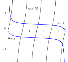
Figure 4: Left-hand sides (black) and right-hand sides (blue) of equations (27) for $\alpha=0.7+0.6i$, $n=8$, $1\leq j\leq n$. Notice that $[0,\pi]$ is divided into $8$ equal subintervals, and each subinterval corresponds to its proper equation.

Proposition 5 implies Theorems 1 and 2 for $|\alpha|<1$.

Recall that $\eta$ is defined by (4). A straightforward computation yields

$$\eta_{\alpha,j}^{\prime}(x)=-\frac{2k_{\alpha}\left(1+\frac{(-1)^{j+1}k_{\alpha}\cot(x)}{\sqrt{k_{\alpha}^{2}\cot^{2}(x)+l_{\alpha}^{2}}}\right)\left(1+\cot^{2}(x)\right)}{1+\left((-1)^{j+1}k_{\alpha}\cot(x)+\sqrt{k_{\alpha}^{2}\cot^{2}(x)+l_{\alpha}^{2}}\right)^{2}}.$$ (28)

Proposition 6.

Let $\alpha\in\mathbb{C}$, $|\alpha|\neq 1$, $j\in\mathbb{Z}$. Then each derivative of $\eta_{\alpha,j}$ is a bounded function on $(0,\pi)$. In particular, for every $x$ in $(0,\pi)$,

$$|\eta_{\alpha,j}^{\prime}(x)|\leq\frac{4(|\alpha|+1)}{||\alpha|-1|}.$$ (29)

Proof.

By (28), $\eta_{\alpha,j}^{\prime}$ is analytic in a neighborhood of $x$, for any $x$ in $(0,\pi)$. Moreover, for $0<x<\pi/2$,

$$\eta_{\alpha,j}^{\prime}(x)=-\frac{2k_{\alpha}\left(1+\frac{(-1)^{j+1}k_{\alpha}}{\sqrt{k_{\alpha}^{2}+l_{\alpha}^{2}\tan^{2}(x)}}\right)\left(1+\tan^{2}(x)\right)}{\tan^{2}(x)+\left((-1)^{j+1}k_{\alpha}+\sqrt{k_{\alpha}^{2}+l_{\alpha}^{2}\tan^{2}(x)}\right)^{2}},$$

and for $\pi/2<x<\pi$, $\eta_{\alpha,j}^{\prime}(x)$ has a similar expression, with $(-1)^{j}$ instead of $(-1)^{j+1}$. Hence, $\eta_{\alpha,j}^{\prime}$ has an analytic extension to a certain open set in the complex plane containing the segment $[0,\pi]$. Therefore, this function and all their derivatives are bounded on $(0,\pi)$.

An explicit upper bound for $|\eta_{\alpha,j}^{\prime}|$ follows directly from (28). Let us denote $\cot(x)$ by $t$ and explain briefly how to “supress” the unbounded factor $1+t^{2}$ appearing in the numerator of (28). If $(-1)^{k+1}k_{\alpha}t\geq 0$, then the denominator of (28) is sufficiently large:

$$1+\left((-1)^{j+1}k_{\alpha}t+\sqrt{k_{\alpha}^{2}t^{2}+l_{\alpha}^{2}}\right)^{2}\geq k_{\alpha}^{2}t^{2}+l_{\alpha}^{2}\geq k_{\alpha}^{2}t^{2}+k_{\alpha}^{2}=k_{\alpha}^{2}(t^{2}+1).$$

If $(-1)^{k}k_{\alpha}t\geq 0$, then a factor in the numerator of (28) is sufficiently small:

$$1+\frac{(-1)^{j+1}k_{\alpha}t}{\sqrt{k_{\alpha}^{2}t^{2}+1}}=\frac{l_{\alpha}^{2}}{\left(\sqrt{k_{\alpha}^{2}t^{2}+l_{\alpha}^{2}}+(-1)^{j}k_{\alpha}t\right)\sqrt{k_{\alpha}^{2}t^{2}+l_{\alpha}^{2}}}\leq\frac{l_{\alpha}^{2}}{k_{\alpha}^{2}(t^{2}+1)}.$$

In both cases, we easily obtain (29). ∎

Let $f_{\alpha,n,j}$ be the function defined on $[0,\pi]$ by the right-hand side of (7):

$$f_{\alpha,n,j}(x)\coloneqq\frac{j\pi+\eta_{\alpha,j}(x)}{n}.$$ (30)

Proposition 7.

Let $|\alpha|<1$, $N_{1}(\alpha)$ be defined by (8), $n>N_{1}(\alpha)$, and $1\leq j\leq n$. Then $f_{\alpha,n,j}$ is contractive in $[0,\pi]$, and its fixed point belongs to $I_{n,j}$.

Proof.

Since the function $\eta_{\alpha,j}$ takes values in $[-\pi,0]$ and its derivative is bounded by (29), it is easy to see that $f_{\alpha,n,j}(x)\in[0,\pi]$ for every $x$ in $[0,\pi]$, and

$$|f^{\prime}_{\alpha,n,j}(x)|\leq\frac{N_{1}(\alpha)}{n}<1.$$

Moreover, the assumption $|\alpha|<1$ implies that $\eta_{\alpha,j}(0)=0$ and $\eta_{\alpha,j}(\pi)=-\pi$. Therefore

$$f_{\alpha,n,j}(0)>0,\qquad f_{\alpha,n,j}(\pi)<\pi.$$

So, if $x$ is the fixed point of $f_{\alpha,n,j}$, then $0<x<\pi$. Thus, $-\pi<\eta_{\alpha,j}(x)<0$ and

$$x=f_{\alpha,n,j}(x)=\frac{j\pi+\eta_{\alpha,j}(x)}{n}\in\left(\frac{(j-1)\pi}{n},\frac{j\pi}{n}\right)=I_{n,j}.$$

In particular, this implies that the fixed point of $f_{\alpha,n,j}$ coincides with $\vartheta_{\alpha,n,j}$. ∎

Proposition 8.

Let $\alpha\in\mathbb{C}$, $|\alpha|<1$. Then there exists $C_{3}(\alpha)>0$ such that for $n$ large enough and $1\leq j\leq n$,

$$\vartheta_{\alpha,n,j}=\frac{j\pi}{n}+\frac{\eta_{\alpha,j}\left(\frac{j\pi}{n}\right)}{n}+\frac{\eta_{\alpha,j}\left(\frac{j\pi}{n}\right)\eta_{\alpha,j}^{\prime}\left(\frac{j\pi}{n}\right)}{n^{2}}+r_{\alpha,n,j},$$ (31)

where $|r_{\alpha,n,j}|\leq\frac{C_{3}(\alpha)}{n^{3}}$.

Proof.

Theorem 1 assures the initial approximation $\vartheta_{\alpha,n,j}=j\pi/n+O(1/n)$. Substitute it into the right-hand side of (7) and expand $\eta_{\alpha,j}$ by Taylor’s formula around $j\pi/n$:

$$\vartheta_{\alpha,n,j}=\frac{j\pi+\eta_{\alpha,j}\left(\frac{j\pi}{n}+O\left(\frac{1}{n}\right)\right)}{n}=\frac{j\pi}{n}+\frac{\eta_{\alpha,j}\left(\frac{j\pi}{n}\right)}{n}+O_{\alpha}\left(\frac{1}{n^{2}}\right).$$

Iterate once again in (7):

$$\vartheta_{\alpha,n,j}=\frac{j\pi+\eta_{\alpha,j}\left(\frac{j\pi}{n}+\frac{\eta_{\alpha,j}\left(\frac{j\pi}{n}\right)}{n}+O_{\alpha}\left(\frac{1}{n^{2}}\right)\right)}{n}.$$

Expanding $\eta_{\alpha,j}$ around $j\pi/n$ with two exact term and estimating the residue term with Proposition 6 we obtain the desired result. ∎

Theorem 3 follows from Proposition 8: we just evaluate $g$ at the expression (31) and expand it by Taylor’s formula around $j\pi/n$. See [2] for a more general scheme.

The next proposition can be seen as a particular case of [24], therefore we do not include the proof.

Proposition 9 (the eigenvectors for weak perturbations).

Let $\alpha\in\mathbb{C}$, $|\alpha|<1$, $n\geq 3$, $1\leq j\leq n$. Then the vector $v_{\alpha,n,j}=\bigl{[}v_{\alpha,n,j,k}\bigr{]}_{k=1}^{n}$ with components

$$v_{\alpha,n,j,k}\coloneqq\sin(k\vartheta_{\alpha,n,j})+\overline{\alpha}\sin((n-k)\vartheta_{\alpha,n,j})$$ (32)

is an eigenvector of the matrix $A_{\alpha,n}$ associated to the eigenvalue $\lambda_{\alpha,n,j}$.

4 Case $\boldsymbol{|\alpha|=1}$

For $|\alpha|=1$, the eigenvalues of $A_{\alpha,n}$ can be computed explicitly.

Proposition 10.

Let $\alpha\in\mathbb{C}$, $|\alpha|=1$, $\alpha\neq\pm 1$, $n\geq 3$, and $1\leq j\leq n$. Then $\lambda_{\alpha,n,j}=g(\vartheta_{\alpha,n,j})$, where

$$\vartheta_{\alpha,n,j}=\frac{j\pi}{n}-\frac{2}{n}\arctan\left(l_{\alpha}^{(-1)^{j}}\right).$$ (33)

Furthermore, $\vartheta_{\alpha,n,j}\in I_{n,j}$, and the vector with components (32) is an eigenvector of $A_{\alpha,n}$ associated to $\lambda_{\alpha,n,j}$.

Proof.

The condition about $\alpha$ implies that $k_{\alpha}=0$. In this case, the functions $\eta_{\alpha,1}$ and $\eta_{\alpha,2}$ are just constants:

$$\eta_{\alpha,j}(x)=-2\arctan\left(l_{\alpha}^{(-1)^{j}}\right),$$

and the characteristic equation (7) simplifies to the direct formula (33). ∎

Proposition 10 implies Theorems 1, 2, and 3, in the case $|\alpha|=1$ and $\alpha\neq\pm 1$.

For $\alpha=\pm 1$, the situation is different: the definition of $\eta_{\alpha,j}$ does not make sense, each number $\vartheta_{\alpha,n,j}$ coincides with one of the extremes of $I_{n,j}$, and most of the eigenvalues are double.

Proposition 11.

Let $\alpha=1$, $n\geq 3$, and $1\leq j\leq n$. Then $\lambda_{1,n,j}=g(\vartheta_{1,n,j})$, where

$$\vartheta_{1,n,j}=\left(j-\frac{1-(-1)^{j}}{2}\right)\frac{\pi}{n}=\begin{cases}\displaystyle\vphantom{\int_{0}^{1}}\frac{2q\pi}{n},&j=2q,\\[4.30554pt] \displaystyle\vphantom{\int_{0}^{1}}\frac{2q\pi}{n},&j=2q+1.\end{cases}$$ (34)

The vector $v_{1,n,j}=[v_{1,n,j,k}]_{k=1}^{n}$ with components

$$v_{1,n,j,k}\coloneqq\sin\left(k\vartheta_{1,n,j}+\frac{(1-(-1)^{j})\pi}{4}\right)=\begin{cases}\displaystyle\vphantom{\int_{0}^{1}}\sin\frac{2kq\pi}{n},&j=2q,\\[4.30554pt] \displaystyle\vphantom{\int_{0}^{1}}\cos\frac{2kq\pi}{n},&j=2q+1,\end{cases}$$ (35)

is an eigenvector of $A_{1,n}$ associated to $\lambda_{1,n,j}$.

Proof.

The numbers $\vartheta_{1,n,j}$ can be found by passing to the limit $\alpha\to 1^{-}$ in (7). The equalities $A_{1,n}v_{1,n,j}=\lambda_{1,n,j}v_{1,n,j}$ are easy to verify directly. ∎

The formulas for the eigenvalues of $A_{1,n}$ also follow from the theory of circulant matrices, since the matrix $A_{1,n}$ is circulant. Notice that

$$\lambda_{1,n,1}<\lambda_{1,n,2}=\lambda_{1,n,3}<\lambda_{1,n,4}=\lambda_{1,n,5}<\ldots,$$

i.e. each of the eigenvalues $\lambda_{1,n,2}$, $\lambda_{1,n,4}$, etc. is double and has two linearly independent eigenvectors.

Proposition 12.

Let $\alpha=-1$, $n\geq 3$, and $1\leq j\leq n$. Then $\lambda_{-1,n,j}=g(\vartheta_{-1,n,j})$, where

$$\vartheta_{-1,n,j}=\left(j-\frac{1+(-1)^{j}}{2}\right)\frac{\pi}{n}=\begin{cases}\displaystyle\vphantom{\int_{0}^{1}}\frac{(2q-1)\pi}{n},&j=2q-1,\\[4.30554pt] \displaystyle\vphantom{\int_{0}^{1}}\frac{(2q-1)\pi}{n},&j=2q.\end{cases}$$ (36)

The vector $v_{-1,n,j}=[v_{-1,n,j,k}]_{k=1}^{n}$ with components

$$v_{-1,n,j,k}\coloneqq\sin\left(k\vartheta_{-1,n,j}+\frac{(1+(-1)^{j})\pi}{4}\right)=\begin{cases}\displaystyle\vphantom{\int_{0}^{1}}\sin\frac{k(2q-1)\pi}{n},&j=2q-1,\\[4.30554pt] \displaystyle\vphantom{\int_{0}^{1}}\cos\frac{k(2q-1)\pi}{n},&j=2q,\end{cases}$$ (37)

is an eigenvector of $A_{-1,n}$ associated to $\lambda_{-1,n,j}$.

Proof.

Similar to the proof of Proposition 11. ∎

By Proposition 12,

$$\lambda_{-1,n,1}=\lambda_{-1,n,2}<\lambda_{-1,n,3}=\lambda_{-1,n,4}<\ldots,$$

i.e. each of the eigenvalues $\lambda_{-1,n,1}$, $\lambda_{-1,n,3}$, etc. is double and has two linearly independent eigenvectors.

5 Proofs for the case of strong perturbations

Let us show that for $|\alpha|>1$, $n$ large enough and $2\leq j\leq n-1$, the situation is nearly the same as in Proposition 7. Recall that $N_{1}(\alpha)$ and $f_{\alpha,n,j}$ are defined by (8) and (30).

Proposition 13.

Let $|\alpha|>1$, $n>N_{1}(\alpha)$, and $2\leq j\leq n-1$. Then $f_{\alpha,n,j}$ is contractive on $[0,\pi]$. If $x$ is the fixed point of $f_{\alpha,n,j}$, then $x\in I_{n,j}$, and $g(x)$ is an eigenvalue of $A_{\alpha,n}$.

Proof.

Inequality (29) and the assumption $n\geq N_{1}(\alpha)$ imply that $f_{\alpha,n,j}$ is contractive on $[0,\pi]$. Unlike in the case of weak perturbations, in the case $|\alpha|>1$ we have

$$\eta_{\alpha,j}(0)=-\pi,\qquad\eta_{\alpha,j}(\pi)=0.$$ (38)

Now the condition $2\leq j\leq n-1$ assures that $0$ and $\pi$ are not fixed points of $f_{\alpha,n,j}$:

$$f_{\alpha,n,j}(0)=\frac{j\pi-\pi}{n}>0,\qquad f_{\alpha,n,j}(\pi)=\frac{j\pi+0}{n}<\pi.$$

Let $x$ be the fixed point of $f_{\alpha,n,j}$. Then $0<x<\pi$. Hence $-\pi<\eta_{\alpha,j}(x)<0$ and $x=f_{\alpha,n,j}(x)\in I_{n,j}$. ∎

Proposition 14.

Let $|\alpha|>1$ and $n>N_{1}(\alpha)$. Then $0$ and $4$ are not eigenvalues of $A_{\alpha,n}$.

Proof.

Formulas from the proof of Proposition 2 and the assumption $n>N_{1}(\alpha)$ easily imply that $\det(\lambda I_{n}-A_{\alpha,n})\neq 0$ for $\lambda\in\{0,4\}$. ∎

If $|\alpha|>1$ and $n\geq N_{1}(\alpha)$, then the functions $f_{\alpha,n,1}$ and $f_{\alpha,n,n}$ are contractive, but their fixed points are $0$ and $\pi$. The corresponding values of $g$, i.e. the points $0$ and $4$, are not eigenvalues of $A_{\alpha,n}$. Hence, for $|\alpha|>1$ and $n$ large enough, the trigonometric change of variables $\lambda=g(x)$ with real $x$ allows us to find only $n-2$ eigenvalues. In order to find the eigenvalues outside of $[0,4]$, we will use the change of variables $\lambda=g_{-}(x)$ or $\lambda=g_{+}(x)$, defined by (12).

Proposition 15.

For $x>0$ and $\lambda=g_{-}(x)$, the equation $\det(\lambda I_{n}-A_{\alpha,n})=0$ is equivalent to

$$\tanh(x)=\frac{2(|\alpha|^{2}-1)\tanh\frac{nx}{2}}{|\alpha+1|^{2}\tanh^{2}\frac{nx}{2}+|\alpha-1|^{2}}.$$ (39)

For $x>0$ and $\lambda=g_{+}(x)$, the equation $\det(\lambda I_{n}-A_{\alpha,n})=0$ is equivalent to

$$\tanh(x)=\frac{2(|\alpha|^{2}-1)\tanh\frac{nx}{2}}{|\alpha+(-1)^{n}|^{2}\tanh^{2}\frac{nx}{2}+|\alpha-(-1)^{n}|^{2}}.$$ (40)

Proof.

For $\lambda=g_{-}(x)=2-2\cosh(x)$, we apply (21) and (20). After some simple transformations,

$$\det(g_{-}(x)I_{n}-A_{\alpha,n}) =\frac{(-1)^{n}}{1-\tanh^{2}\frac{nx}{2}}\biggl{(}|\alpha+1|^{2}\tanh^{2}\frac{nx}{2}$$ (41)

$$\quad-2(|\alpha|^{2}-1)\tanh\frac{nx}{2}\,\coth(x)+|\alpha-1|^{2}\biggr{)}.$$

This expression for the characteristic polynomial yields (39). The proof of (40) is analogous. ∎

Remark 1.

In formula (25), $\tan\frac{nx}{2}$ is rapidly oscillating and $\cot(x)$ is much slower, therefore we solve (25) for $\tan\frac{nx}{2}$. The situation in (41) is different: if $x$ is separated from zero and $n$ is large enough, then $\tanh\frac{nx}{2}$ is almost a constant, and we prefer to solve (41) for $\tanh(x)$.

In what follows, we restrict ourselves to the analysis of the equation (39), because (40) is similar. Define $\psi_{\alpha}\colon[0,1]\to[0,+\infty)$ by

$$\psi_{\alpha}(t)\coloneqq\frac{2(|\alpha|^{2}-1)t}{|\alpha+1|^{2}t^{2}+|\alpha-1|^{2}}.$$ (42)

Notice that

$$\psi_{\alpha}(1)=\frac{2(|\alpha|^{2}-1)}{|\alpha+1|^{2}+|\alpha-1|^{2}}=\frac{|\alpha|^{2}-1}{|\alpha|^{2}+1}=\tanh(\log|\alpha|).$$ (43)

We are going to construct explicitly a left neighborhood of $1$ where the values of $\psi_{\alpha}$ are close enough to $\tanh(\log|\alpha|)$.

Lemma 1.

Let $|\alpha|>1$. Then for every $t$ with

$$1-\frac{|\alpha|-1}{(|\alpha|+1)^{3}}\leq t\leq 1,$$ (44)

the following inequalities hold:

$$|\psi_{\alpha}^{\prime}(t)|\leq 1,$$ (45)

$$\tanh\frac{\log|\alpha|}{2}\leq\psi_{\alpha}(t)\leq\tanh\frac{3\log|\alpha|}{2},$$ (46)

$$1-\psi_{\alpha}^{2}(t)\geq\frac{2}{(|\alpha|+1)^{3}}.$$ (47)

Proof.

The proof is quite elementary, therefore we will only mention the main steps. Assumption (44) implies that

$$1-t^{2}\leq\frac{2(|\alpha|-1)}{(|\alpha|+1)^{3}},\qquad|\alpha+1|^{2}t^{2}+|\alpha-1|^{2}\geq\frac{2(|\alpha|^{3}+|\alpha|^{2}+2)}{|\alpha|+1}.$$

With these estimates we obtain (45). After that, the mean value theorem and (43) provide (46). Inequality (47) follows from (46). ∎

Recall that $N_{2}(\alpha)$ and $S_{\alpha}$ are given by (11) and (15). Define $h_{\alpha,n}$ on $S_{\alpha}$ as the right-hand side of (13):

$$h_{\alpha,n}(x)\coloneqq\operatorname{arctanh}\frac{2(|\alpha|^{2}-1)\tanh\frac{nx}{2}}{|\alpha+1|^{2}\tanh^{2}\frac{nx}{2}+|\alpha-1|^{2}}.$$

Proposition 16.

Let $\alpha\in\mathbb{C}$, $|\alpha|>1$, and $n>N_{2}(\alpha)$. Then $h_{\alpha,n}$ is contractive on $S_{\alpha}$, and its fixed point is the solution of (39).

Proof.

We represent $h_{\alpha,n}$ as the following composition:

$$h_{\alpha,n}(x)=\operatorname{arctanh}\left(\psi_{\alpha}\left(\tanh\frac{nx}{2}\right)\right).$$

For $x$ in $S_{\alpha}$, denote $\tanh\frac{nx}{2}$ by $t$. Then

$$1-t\leq 2e^{-nx}\leq 2e^{-N_{2}(\alpha)\frac{\log|\alpha|}{2}}<\frac{|\alpha|-1}{(|\alpha|+1)^{3}}.$$

Therefore, by (47) we have $\psi_{\alpha}(\tanh\frac{nx}{2})<1$, and the definition of $h_{\alpha,n}$ makes sense. By (46), $h_{\alpha,n}$ takes values in $S_{\alpha}$. Estimate from above the derivative of $h_{\alpha,n}$ using (47), (45), and the elementary inequality $ue^{-u}\leq 1/e$:

$$|h_{\alpha,n}^{\prime}(x)| \leq\frac{|\psi_{\alpha}^{\prime}(t)|}{1-\psi_{\alpha}^{2}(t)}\cdot\frac{n}{2\cosh^{2}\frac{nx}{2}}\leq(|\alpha|+1)^{3}ne^{-nx}$$

$$\leq(|\alpha|+1)^{3}ne^{-\frac{n\log|\alpha|}{2}}=(|\alpha|+1)^{3}ne^{-\frac{n\log|\alpha|}{4}}e^{-\frac{n\log|\alpha|}{4}}$$

$$\leq(|\alpha|+1)^{3}\cdot\frac{4}{\log|\alpha|}\cdot\frac{\log|\alpha|}{(|\alpha|+1)^{5}}=\frac{4}{(|\alpha|+1)^{2}}<1.$$

Obviously, the fixed point of $h_{\alpha,n}$ is the solution of (13) and (39). ∎

At the moment, we have proven Theorems 4 and 5. Asymptotic formulas for $\lambda_{\alpha,n,j}$ with $|\alpha|>1$ and $2\leq j\leq n-1$ can be justified in the same manner as for $|\alpha|<1$, and we are left to prove the exponential convergence (17) and (18).

Proposition 17.

Let $|\alpha|>1$ and $C_{4}(\alpha)\coloneqq|\alpha|^{3}e^{\frac{|\alpha|^{3}}{\log|\alpha|}}$. Then for all $n\geq N_{2}(\alpha)$

$$\bigl{|}\vartheta_{\alpha,n,1}-\log|\alpha|\bigr{|}\leq\frac{C_{4}(\alpha)}{|\alpha|^{n}}.$$ (48)

Proof.

For brevity, put $x=\vartheta_{\alpha,n,1}$. Apply the mean value theorem to $\psi_{\alpha}$, taking into account (45):

$$\bigl{|}\tanh(x)-\tanh(\log|\alpha|)\bigr{|}=\left|\psi_{\alpha}\left(\tan\frac{nx}{2}\right)-\psi_{\alpha}(1)\right|\leq 1-\tan\frac{nx}{2}\leq 2e^{-nx}.$$

On the other hand, apply the mean value theorem to $\tanh$:

$$|\tanh(x)-\tanh(\log|\alpha|)|\geq\frac{\bigl{|}x-\log|\alpha|\bigr{|}}{\cosh^{2}\frac{3\log|\alpha|}{2}}\geq\frac{2}{|\alpha|^{3}}\bigl{|}x-\log|\alpha|\bigr{|}.$$

From this chain of inequalities,

$$|x-\log|\alpha||\leq|\alpha|^{3}e^{-nx}.$$ (49)

We already know from Proposition 16 that $x\geq\frac{\log|\alpha|}{2}$. Thus,

$$x\geq\log|\alpha|-|\alpha|^{3}e^{-\frac{n\log|\alpha|}{2}}.$$

Using the elementary inequality $ue^{-u}\leq 1/e$ we get

$$nx\geq n\log|\alpha|-|\alpha|^{3}\,ne^{-\frac{n\log|\alpha|}{2}}\geq n\log|\alpha|-\frac{|\alpha|^{3}}{\log|\alpha|}.$$ (50)

By (49) and (50), inequality (48) holds. ∎

In a similar manner, $|\vartheta_{\alpha,n,n}-\log|\alpha||\leq C_{4}(\alpha)/|\alpha|^{n}$. Since the derivatives of $g_{-}$ and $g_{+}$ are bounded on $\left[0,\frac{3}{2}\log|\alpha|\right]$, we get limit relations (17) and (18). Thereby we have proven the parts of Theorem 6 related to the extreme eigenvalues $\lambda_{\alpha,n,1}$ and $\lambda_{\alpha,n,n}$.

Proposition 18 (the eigenvectors for strong perturbations).

Let $\alpha\in\mathbb{C}$, $|\alpha|>1$, $n\geq N(\alpha)$. Then the vectors $v_{\alpha,n,1}\coloneqq[v_{\alpha,n,1,k}]_{k=1}^{n}$ and $v_{\alpha,n,n}\coloneqq[v_{\alpha,n,n,k}]_{k=1}^{n}$ with components

$$v_{\alpha,1,n,k} =\sinh(k\vartheta_{\alpha,n,1})+\overline{\alpha}\sinh((n-k)\vartheta_{\alpha,n,1}),$$ (51)

$$v_{\alpha,n,n,k} =(-1)^{k}\sinh(k\vartheta_{\alpha,n,n}))+(-1)^{k+n}\,\overline{\alpha}\sinh((n-k)\vartheta_{\alpha,n,n}),$$ (52)

are the eigenvectors of the matrix $A_{\alpha,n}$ associated to the eigenvalues $\lambda_{\alpha,1,n}$ and $\lambda_{\alpha,n,n}$, respectively. For $2\leq j\leq n-1$, the vector $v_{\alpha,n,j}$ defined by (32) is an eigenvector of $A_{\alpha,n}$ associated to the eigenvalue $\lambda_{\alpha,n,j}$.

Remark 2.

It is possible to show that for a fixed $\alpha$ with $|\alpha|>1$ and large values of $n$, the norms of the vectors $v_{\alpha,n,1}$ and $v_{\alpha,n,n}$, given by (51) and (52), grow as $|\alpha|^{n}$. In order to avoid large numbers, we recommend to divide each component of these vectors by $|\alpha|^{n}$.

6 Numerical experiments

We use the following notation for different approximations of the eigenvalues.

• $\lambda_{\alpha,n,j}^{\text{gen}}$ are the eigenvalues computed in Sagemath by general algorithms, with double-precision arithmetic.

• $\lambda_{\alpha,n,j}^{\text{fp}}$ are the eigenvalues computed by formulas of Theorems 2 and 5, i.e. solving the equations (7),  (13), and (14) by the fixed point iteration; these computations are performed in the high-precision arithmetic with $3322$ binary digits ($\approx 1000$ decimal digits). Using $\lambda_{\alpha,n,j}^{\text{fp}}$ we compute $v_{\alpha,n,j}$ by (32), (51), and (52).

• $\lambda_{\alpha,n,j}^{\text{asympt}}$ are the approximations given by (9) and (19).

In (13) and (14), we compute $\tanh\frac{nx}{2}$ as $1-2e^{-nx}/(1+e^{-nx})$, because $nx/2$ can be large and the standard formula for $\tanh$ can produce overflows (“NaN”).

We have constructed a large series of examples with random values of $\alpha$ and $n$. In all these examples, we have obtained

$$\max_{1\leq j\leq n}|\lambda_{\alpha,n,j}^{\text{gen}}-\lambda_{\alpha,n,j}^{\text{fp}}|<2\cdot 10^{-13},\qquad\frac{\|A_{\alpha,n}v_{\alpha,n,j}-\lambda_{\alpha,n,j}^{\text{fp}}v_{\alpha,n,j}\|}{\|v_{\alpha,n,j}\|}<10^{-996}.$$

This means that the exact formulas from Theorems 2 and 5 are fulfilled up to the rounding errors. Theorems 1 and 4 can be viewed as simple corollaries from Theorems 2 and 5, so they do not need additional tests. For Theorems 3 and 6, we have computed the errors

$$R_{\alpha,n,j}\coloneqq\lambda_{\alpha,n,j}^{\text{asympt}}-\lambda_{\alpha,n,j}^{\text{fp}}$$

and their maximums $\|R_{\alpha,n}\|_{\infty}=\max_{1\leq j\leq n}|R_{\alpha,n,j}|$. Tables 1 and 2 show that these errors indeed can be bounded by $C_{1}(\alpha)/n^{3}$, and $C_{1}(\alpha)$ has to take bigger values when $|\alpha|$ is close to $1$.

Table 1: Values of $\|R_{\alpha,n}\|_{\infty}$ and $n^{3}\|R_{\alpha,n}\|_{\infty}$ for some $|\alpha|<1$.

$$\begin{array}[]{|c|c|c|}\hline\cr\vrule\lx@intercol\hfil\vphantom{\int_{0_{0}}^{1^{1}}}\alpha=-0.3+0.5i,\quad|\alpha|\approx 0.58\hfil\lx@intercol\vrule\lx@intercol\\ \hline\cr\vphantom{\int_{0_{0}}^{1^{1}}}n&\|R_{\alpha,n}\|_{\infty}&\mbox{}\ \mbox{}{}n^{3}\|R_{\alpha,n}\|_{\infty}\mbox{}\ \mbox{}{}\\ \hline\cr\vphantom{\int_{0}^{1}}64&1.76\times 10^{-4}&46.05\\ \vphantom{\int_{0}^{1}}128&2.49\times 10^{-5}&52.13\\ \vphantom{\int_{0}^{1}}256&3.29\times 10^{-6}&55.12\\ \vphantom{\int_{0}^{1}}512&4.22\times 10^{-7}&56.58\\ \vphantom{\int_{0}^{1}}1024&5.34\times 10^{-8}&57.31\\ \vphantom{\int_{0}^{1}}2048&6.71\times 10^{-9}&57.67\\ \vphantom{\int_{0}^{1}}\mbox{}\ \mbox{}{}4096\mbox{}\ \mbox{}{}&\mbox{}\ \mbox{}{}8.42\times 10^{-10}\mbox{}\ \mbox{}{}&\mbox{}\ \mbox{}{}57.84\mbox{}\ \mbox{}{}\\ \vphantom{\int_{0}^{1}}\mbox{}\ \mbox{}{}8192\mbox{}\ \mbox{}{}&\mbox{}\ \mbox{}{}1.05\times 10^{-10}\mbox{}\ \mbox{}{}&\mbox{}\ \mbox{}{}57.93\mbox{}\ \mbox{}{}\\ \hline\cr\end{array}\qquad\begin{array}[]{|c|c|c|}\hline\cr\vrule\lx@intercol\hfil\vphantom{\int_{0_{0}}^{1^{1}}}\alpha=0.7+0.6i,\quad|\alpha|\approx 0.92\hfil\lx@intercol\vrule\lx@intercol\\ \hline\cr\vphantom{\int_{0_{0}}^{1^{1}}}n&\|R_{\alpha,n}\|_{\infty}&\mbox{}\ \mbox{}{}n^{3}\|R_{\alpha,n}\|_{\infty}\mbox{}\ \mbox{}{}\\ \hline\cr\vphantom{\int_{0}^{1}}64&1.02\times 10^{-3}&266.71\\ \vphantom{\int_{0}^{1}}128&1.59\times 10^{-4}&333.02\\ \vphantom{\int_{0}^{1}}256&2.24\times 10^{-5}&376.61\\ \vphantom{\int_{0}^{1}}512&2.99\times 10^{-6}&401.28\\ \vphantom{\int_{0}^{1}}1024&3.86\times 10^{-7}&414.29\\ \vphantom{\int_{0}^{1}}2048&4.90\times 10^{-8}&420.94\\ \vphantom{\int_{0}^{1}}\mbox{}\ \mbox{}{}4096\mbox{}\ \mbox{}{}&\mbox{}\ \mbox{}{}6.17\times 10^{-9}\mbox{}\ \mbox{}{}&\mbox{}\ \mbox{}{}424.30\mbox{}\ \mbox{}{}\\ \vphantom{\int_{0}^{1}}\mbox{}\ \mbox{}{}8192\mbox{}\ \mbox{}{}&\mbox{}\ \mbox{}{}7.75\times 10^{-10}\mbox{}\ \mbox{}{}&425.99\\ \hline\cr\end{array}$$

Table 2: Values of $\|R_{\alpha,n}\|_{\infty}$ and $n^{3}\|R_{\alpha,n}\|_{\infty}$ for some $|\alpha|>1$.

$$\begin{array}[]{|c|c|c|}\hline\cr\vrule\lx@intercol\hfil\vphantom{\int_{0_{0}}^{1^{1}}}\alpha=2+i,\quad|\alpha|\approx 2.23\hfil\lx@intercol\vrule\lx@intercol\\ \hline\cr\vphantom{\int_{0_{0}}^{1^{1}}}n&\|R_{\alpha,n}\|_{\infty}&\mbox{}\ \mbox{}{}n^{3}\|R_{\alpha,n}\|_{\infty}\mbox{}\ \mbox{}{}\\ \hline\cr\vphantom{\int_{0}^{1}}64&1.55\times 10^{-4}&40.59\\ \vphantom{\int_{0}^{1}}128&2.15\times 10^{-5}&45.18\\ \vphantom{\int_{0}^{1}}256&2.82\times 10^{-6}&47.33\\ \vphantom{\int_{0}^{1}}512&3.60\times 10^{-7}&48.36\\ \vphantom{\int_{0}^{1}}1024&4.55\times 10^{-8}&48.86\\ \vphantom{\int_{0}^{1}}2048&5.72\times 10^{-9}&49.10\\ \vphantom{\int_{0}^{1}}\mbox{}\ \mbox{}{}4096\mbox{}\ \mbox{}{}&\mbox{}\ \mbox{}{}7.16\times 10^{-10}\mbox{}\ \mbox{}{}&\mbox{}\ \mbox{}{}49.22\mbox{}\ \mbox{}{}\\ \vphantom{\int_{0}^{1}}\mbox{}\ \mbox{}{}8192\mbox{}\ \mbox{}{}&\mbox{}\ \mbox{}{}8.97\times 10^{-11}\mbox{}\ \mbox{}{}&\mbox{}\ \mbox{}{}49.29\mbox{}\ \mbox{}{}\\ \hline\cr\end{array}\qquad\begin{array}[]{|c|c|c|}\hline\cr\vrule\lx@intercol\hfil\vphantom{\int_{0_{0}}^{1^{1}}}\alpha=0.8-0.7i,\quad|\alpha|\approx 1.06\hfil\lx@intercol\vrule\lx@intercol\\ \hline\cr\vphantom{\int_{0_{0}}^{1^{1}}}n&\|R_{\alpha,n}\|_{\infty}&\mbox{}\ \mbox{}{}n^{3}\|R_{\alpha,n}\|_{\infty}\mbox{}\ \mbox{}{}\\ \hline\cr\vphantom{\int_{0}^{1}}64&2.19\times 10^{-4}&57.51\\ \vphantom{\int_{0}^{1}}128&2.19\times 10^{-5}&45.90\\ \vphantom{\int_{0}^{1}}256&1.40\times 10^{-5}&235.36\\ \vphantom{\int_{0}^{1}}512&2.99\times 10^{-6}&401.90\\ \vphantom{\int_{0}^{1}}1024&4.55\times 10^{-7}&488.25\\ \vphantom{\int_{0}^{1}}2048&6.16\times 10^{-8}&528.84\\ \vphantom{\int_{0}^{1}}\mbox{}\ \mbox{}{}4096\mbox{}\ \mbox{}{}&\mbox{}\ \mbox{}{}7.98\times 10^{-9}\mbox{}\ \mbox{}{}&\mbox{}\ \mbox{}{}548.04\mbox{}\ \mbox{}{}\\ \vphantom{\int_{0}^{1}}\mbox{}\ \mbox{}{}8192\mbox{}\ \mbox{}{}&\mbox{}\ \mbox{}{}1.01\times 10^{-9}\mbox{}\ \mbox{}{}&\mbox{}\ \mbox{}{}557.32\mbox{}\ \mbox{}{}\\ \hline\cr\end{array}$$

We have also tested (17) and (18). As $n$ grows, $|\alpha|^{n}|R_{\alpha,n,1}|$ and $|\alpha|^{n}|R_{\alpha,n,n}|$ approach rapidly the same limit value depending on $\alpha$. For example,

$$\text{for}\ \alpha=2+i, \lim_{n\to\infty}\left(|\alpha|^{n}|R_{\alpha,n,1}|\right)\approx 2.86,$$

$$\text{for}\ \alpha=0.8-0.7i, \lim_{n\to\infty}\left(|\alpha|^{n}|R_{\alpha,n,1}|\right)\approx 1.12\cdot 10^{-2}.$$

Acknowledgements.

The research has been supported by CONACYT (Mexico) scholarships and by IPN-SIP project 20200650 (Instituto Politécnico Nacional, Mexico). We are grateful to Óscar García Hernández for his participation on the early stages of this research (we worked with the case $0\leq\alpha<1$).

Sergei M. Grudsky,
grudsky@math.cinvestav.mx,
ReseachID J-5263-2017,
CINVESTAV, Departamento de Matemáticas,
Apartado Postal 07360, Ciudad de México,
Mexico.

Egor A. Maximenko,
emaximenko@ipn.mx,
http://orcid.org/0000-0002-1497-4338,
Instituto Politécnico Nacional, Escuela Superior de Física y Matemáticas,
Apartado Postal 07730, Ciudad de México,
Mexico.

Alejandro Soto-González,
asoto@math.cinvestav.mx,
https://orcid.org/0000-0003-2419-4754,
CINVESTAV, Departamento de Matemáticas,
Apartado Postal 07360, Ciudad de México,
Mexico.

References

- [1] Alexandersson, P.: Schur polynomials, banded Toeplitz matrices and Widom’s formula, Electron. J. Combin. 19, 4, P22 (2012). doi:10.37236/2651.
- [2] Barrera, M., Böttcher, A., Grudsky, S.M., Maximenko, E.A.: Eigenvalues of even very nice Toeplitz matrices can be unexpectedly erratic. In: Böttcher, A., Potts, D., Stollmann, P., Wenzel, D. (eds.) The Diversity and Beauty of Applied Operator Theory. Operator Theory: Advances and Applications, vol. 268, pp. 51–77. Birkhäuser, Cham (2018). doi:10.1007/978-3-319-75996-8_2.
- [3] Bogoya, J.M., Grudsky, S.M., Maximenko, E.A.: Eigenvalues of Hermitian Toeplitz matrices generated by simple-loop symbols with relaxed smoothness. In: Bini, D., Ehrhardt, T., Karlovich, A., Spitkovsky I. (eds.) Large Truncated Toeplitz Matrices, Toeplitz Operators, and Related Topics. Operator Theory: Advances and Applications, vol. 259, pp. 179–212. Birkhäuser, Cham (2017). doi:10.1007/978-3-319-49182-0_11.
- [4] Bogoya, J.M., Böttcher, A., Grudsky, S.M., Maximenko, E.A.: Eigenvalues of Hermitian Toeplitz matrices with smooth simple-loop symbols. J. Math. Anal. Appl. 422, 1308–1334 (2015). doi:10.1016/j.jmaa.2014.09.057.
- [5] Böttcher, A., Bogoya, J.M., Grudsky, S.M., Maximenko, E.A.: Asymptotic formulas for the eigenvalues and eigenvectors of Toeplitz matrices. Sb. Math. 208, 1578–1601 (2017). doi:10.1070/SM8865.
- [6] Böttcher, A., Fukshansky, L., Garcia, S.R., Maharaj, H.: Toeplitz determinants with perturbations in the corners. J. Funct. Anal. 268, 171–193 (2015). doi:10.1016/j.jfa.2014.10.023.
- [7] Böttcher, A., Grudsky, S.M.: Spectral Properties of Banded Toeplitz Matrices, SIAM, Philadelphia (2005)
- [8] Böttcher, A., Silbermann, B.: Introduction to Large Truncated Toeplitz Matrices. Universitext, Springer-Verlag, New York (1999)
- [9] Britanak, V., Yip, P.C., Rao, K.R.: Discrete Cosine and Sine Transforms: General Properties, Fast Algorithms and Integer Approximations. Academic Press, San Diego (2006)
-
[10]
Deift, P., Its, A., Krasovsky, I.:
Eigenvalues of Toeplitz matrices in the bulk of the spectrum.
Bull. Inst. Math. Acad. Sin. (N.S.) 7, 437–461 (2012).
http://web.math.sinica.edu.tw/bulletin_ns/20124/2012401.pdf - [11] Deift, P., Its, A., Krasovsky, I.: Toeplitz matrices and Toeplitz determinants under the impetus of the Ising model. Some history and some recent results. Comm. Pure Appl. Math. 66, 1360–1438 (2013) doi:10.1002/cpa.21467.
- [12] Elouafi, M.: On a relationship between Chebyshev polynomials and Toeplitz determinants. Appl. Math. Comput. 229:1, 27–33 (2014). doi:10.1016/j.amc.2013.12.029.
- [13] Garoni, C., Sierra-Capizzano, S.: Generalized Locally Toeplitz Sequences: Theory and Applications, Volume I. Springer, Cham (2017)
- [14] Gray, R.M.: Toeplitz and Circulant Matrices: A review. Now Publishers Inc, Boston-Delft, in the series Foundations and Trends in Communications and Information Theory, vol. 2, no. 3, pp. 155–239. Now Publishers, Boston–Delft (2005) doi:10.1561/0100000006.
- [15] Grenander, U.; Szegő, G.: Toeplitz Forms and Their Applications. University of California Press, Berkeley, Los Angeles (1958).
- [16] Kulkarni, D., Schmidt, D., Tsui, S.-K.: Eigenvalues of tridiagonal pseudo-Toeplitz matrices. Linear Algebra Appl. 297, 63–80 (1999). doi:10.1016/S0024-3795(99)00114-7.
- [17] Maximenko, E.A., Moctezuma-Salazar, M.A.: Cofactors and eigenvectors of banded Toeplitz matrices: Trench formulas via skew Schur polynomials. Oper. Matrices 11:4, 1149–1169 (2017). doi:10.7153/oam-2017-11-79.
- [18] Noschese, S., Reichel, L.: Eigenvector sensitivity under general and structured perturbations of tridiagonal Toeplitz-type matrices. Numer. Linear Algebra Appl. 26, e2232 (2019). doi:10.1002/nla.2232.
- [19] Tilli, P.: Locally Toeplitz sequences: spectral properties and applications. Linear Algebra Appl. 278, 91–120 (1998). doi:10.1016/S0024-3795(97)10079-9.
- [20] Trench, W.F.: Characteristic polynomials of symmetric rationally generated Toeplitz matrices. Linear Multilinear Alg. 21, 289–296 (1987). doi:10.1080/03081088708817803.
- [21] Tyrtyshnikov, E.E.: A unifying approach to some old and new theorems on distribution and clustering. Linear Algebra Appl. 232, 1–43 (1996). doi:10.1016/0024-3795(94)00025-5.
- [22] Wei, Y., Jiang, X., Jiang, Z., Shon, S.: Determinants and inverses of perturbed periodic tridiagonal Toeplitz matrices. Adv. Differ. Equ. 410 (2019). doi:10.1186/s13662-019-2335-6.
- [23] Widom, H.: Eigenvalue distribution for nonselfadjoint Toeplitz matrices. In: Basor, E.L., Gohberg, I. (eds) Toeplitz Operators and Related Topics. Operator Theory Advances and Applications, vol. 71, pp. 1–8. Birkhäuser, Basel (1994). doi:10.1007/978-3-0348-8543-0_1.
- [24] Yueh, W.-C., Cheng, S.-S.: Explicit eigenvalues and inverses of tridiagonal Toeplitz matrices with four perturbed corners. ANZIAM J. 49, 361–387 (2008). doi:10.1017/S1446181108000102.