ϕΓ
Convexity of the orbit-closed
-numerical range and majorization
Abstract
We introduce and investigate the orbit-closed -numerical range, a natural modification of the -numerical range of an operator introduced for trace-class by Dirr and vom Ende. Our orbit-closed -numerical range is a conservative modification of theirs because these two sets have the same closure and even coincide when is finite rank. Since Dirr and vom Ende’s results concerning the -numerical range depend only on its closure, our orbit-closed -numerical range inherits these properties, but we also establish more.
For selfadjoint, Dirr and vom Ende were only able to prove that the closure of their -numerical range is convex, and asked whether it is convex without taking the closure. We establish the convexity of the orbit-closed -numerical range for selfadjoint without taking the closure by providing a characterization in terms of majorization, unlocking the door to a plethora of results which generalize properties of the -numerical range known in finite dimensions or when has finite rank. Under rather special hypotheses on the operators, we also show the -numerical range is convex, thereby providing a partial answer to the question posed by Dirr and vom Ende.
keywords:
numerical range, -numerical range, convex, trace-class, Toeplitz–Hausdorff Theorem, unitary orbit, Hausdorff distance, essential spectrumPrimary 47A12, 47B15; Secondary 52A10, 52A40, 26D15.
1 Introduction
Herein we let denote a separable complex Hilbert space and the collection of all bounded linear operators on . For , the numerical range is the image of the unit sphere of under the continuous quadratic form , where denotes the inner product on . Of course, the numerical range has a long history but perhaps the most impactful result is the Toeplitz–Hausdorff Theorem which asserts that the numerical range is convex [1, 2]; an intuitive proof is given by Davis in [3]. In this paper we are interested in unitarily invariant generalizations of the numerical range and their associated properties, especially convexity and its relation to majorization.
By considering an alternative definition of the numerical range, some generalizations become readily apparent. Notice that
As Halmos recognized in [4], one could generalize this by fixing and requiring to be a rank- projection. In this way, we arrive at the -numerical range
The normalization constant is actually quite natural; among other things, it ensures is bounded independent of by . In [5, §12], Berger proved a few fundamental facts about the -numerical range including its convexity, as well as the inclusion property . We will see shortly that these convexity and inclusion properties are actually consequences of more general phenomena (see Corollaries 4.6 and 4.7).
In [6], Fillmore and Williams examined , but restricted their attention to the finite dimensional setting. There they established
| (1.1) |
which was generalized by Goldberg and Straus to the -numerical range, as we describe below. Moreover, Fillmore and Williams showed that if is normal, then
| (1.2) |
which says that the extreme points of are contained in the set of averages of -eigenvalues of (allowing repetitions according to multiplicity). This is a clear analogue of the standard fact for numerical ranges that when is normal.
In order to further generalize the -numerical range, yet another new perspective is necessary. The unitary group of acts by conjugation on , and the orbit of an operator under this action is called the unitary orbit. When is any rank- projection (), consists of all rank- projections in . Therefore, if is a rank- projection, then
The above representation of the -numerical range suggests the natural generalization to the -numerical range,
Of course, this requires to make sense, which can be achieved in several different ways, each investigated by various authors. In [7], Westwick considered when is a finite rank selfadjoint operator and proved that is convex by means of Morse theory. When so that , is well-defined for an arbitrary . The -numerical range was first studied in this generality by Goldberg and Straus in [8]. There, they proved a generalization of (1.1) for an arbitrary selfadjoint matrix , which we extend to the infinite dimensional setting in Theorem 4.5. Chi-Kwong Li provides in [9] a comprehensive survey of the properties of the -numerical range in finite dimensions, including the highlights which we now describe. When is selfadjoint the -numerical range is convex, but this may fail even if is normal [7, 10]. However, the -numerical range is always star-shaped relative to the star center [11]. Moreover, there is a set associated to the pair called the -spectrum of which, when is a rank-1 projection, coincides with the usual spectrum of ; Then when is normal and is selfadjoint, [12, Theorem 4], which generalizes (1.2).
In the recent paper [13], Dirr and vom Ende study a generalization of the -numerical range to the infinite dimensional setting. In this case, it again becomes necessary to ensure that the trace is well-defined, which they naturally enforce by requiring to be trace-class. In [13], they prove extensions of some finite dimensional results by means of limiting arguments. As a result of these limiting arguments, all of their major results pertain to the closure of the -numerical range. Dirr and vom Ende prove that is star-shaped and that any element of is a star center [13, Theorem 3.10]. They asked explicitly [13, Open Problem (b)] whether is convex without taking the closure, and we provide a partial answer in Corollary 7.3. Moreover, they show that is convex whenever is selfadjoint111or only slightly more generally, normal with collinear eigenvalues. In this paper, we have many results for selfadjoint , but they generally have trivial unmentioned corollaries for normal with collinear eigenvalues by means of Proposition 3.7(iii). We neglect these slightly more general statements in favor of the selfadjoint ones solely for clarity and simplicity of exposition. or is a rotation and translation of a selfadjoint operator [13, Theorem 3.8]. Additionally, they prove that if are both normal, is compact and the eigenvalues of either or are collinear, then [13, Corollary 3.1].
In this paper we introduce and investigate a natural modification of the -numerical range with trace-class which we call the orbit-closed -numerical range, denoted (see Definition 3.2). The only difference between and is that the former allows which are approximately unitarily equivalent (in trace norm) to , that is,
where . Considering closures of unitary orbits in various operator topologies serves an important purpose and has precedent in the literature, especially in relation to majorization (see the discussion which introduces section 3).
This relatively small difference between and has significant consequences. In particular, for selfadjoint we give a characterization of in terms of majorization (Theorem 4.5) which is an appropriate extension to infinite dimensions of [6, Theorem 1.2] (included herein as (1.1)) and its generalization [8, Theorem 7], and whose proof is inspired by [14, Theorem 2.14]. Because in general , necessarily cannot enjoy this same characterization. Moreover, this majorization characterization of is the backbone of this paper and it provides a gateway to the rest of our major results. One immediate corollary is the convexity of when is selfadjoint (Corollary 4.6) which generalizes and provides an independent and purely operator-theoretic proof of Westwick’s theorem [7] for a finite rank selfadjoint operator. Moreover, to our knowledge our Corollary 4.6 constitutes the only222 In the finite dimensional setting there is an independent proof of Westwick’s theorem due to Poon [15] using a result of Goldberg and Straus [8, Theorem 7]. This proof is similar in spirit to our Corollary 4.6 because it involves majorization. However, it seems to us that the techniques in [15] cannot be used to reprove Westwick’s result in the infinite dimensional setting even for finite rank . We say this because both [15, Lemma 1] and [8, Theorem 7] rely in an essential way on Birkhoff’s Theorem [16]. The dependence of [8, Theorem 7] on Birkhoff’s Theorem is not readily apparent, but can be observed through a careful analysis of the proof of [8, Lemma 7]. independent proof of Westwick’s convexity result in the infinite dimensional setting found in 45 years, which is especially significant because Westwick’s proof used an unusual technique: Morse theory.
In addition, is a conservative modification of in the sense that (see Theorem 3.4), and moreover, if is finite rank, then . Therefore, the orbit-closed -numerical range constitutes an alternate natural extension of the -numerical range to the infinite dimensional (and infinite rank) setting. Moreover, because , all of Dirr and vom Ende’s results (which concern the closure of the -numerical range) are inherited by the orbit-closed -numerical range.
Our main results are summarized in the list below. Here denotes the eigenvalue sequence of a compact operator (see section 2), , denote majorization and submajorization (see Definition 4.1), and denotes the -spectrum (see Definition 6.3). Reference section 2 for any other unfamiliar notation.
-
(i)
if is finite rank (Proposition 3.1).
-
(ii)
(Theorem 3.4).
-
(iii)
The map is continuous (Theorem 3.5).
-
(iv)
If , then (Theorem 4.5).
-
(v)
If , then is convex (Corollary 4.6).
-
(vi)
If and , then (Corollary 4.7).
- (vii)
-
(viii)
For , is closed if for every , , where (Theorem 5.14).
-
(ix)
If , then (Theorem 6.2)
-
(x)
If , normal, then (Theorem 6.8).
-
(xi)
If with , and is diagonalizable, then is convex (Corollary 7.3).
Many of the results listed above are extensions of facts which are known in either the finite dimensional or finite rank setting. However, to our knowledge, (viii) appears to be entirely new.
This paper is structured as follows. In section 2 we specify some notation. Section 3 contains fundamental properties of the orbit-closed -numerical range for general trace-class operators . Then in section 4 we restrict attention to selfadjoint and establish a characterization of the orbit-closed -numerical range in terms of majorization (Theorem 4.5) which is the main theorem that paves the way for all our other primary results; it has as a direct corollary the convexity of the orbit-closed -numerical range (Corollary 4.6). In section 5 we undertake a thorough investigation of points on the boundary , including an analysis specific to the case when is compact in subsection 5.1. We obtain necessary and sufficient conditions for to be closed when is compact and is selfadjoint (Theorem 5.2). Beginning in subsection 5.2 we restrict our attention to positive for the remainder of the paper, and there we provide a sufficient condition for to be closed when (Theorem 5.14). In section 6 we characterize the behavior of the orbit-closed -numerical range under finite direct sums (Theorem 6.2) and prove when is compact normal (Theorem 6.8). Finally, in section 7 we use variations of the Schur–Horn theorem for positive compact operators to prove that the -numerical range is convex when is diagonalizable and is positive with either trivial or infinite dimensional kernel (Corollary 7.3), thereby providing a partial answer to the question [13, Open Problem (b)] posed by Dirr and vom Ende.
2 Notation
Let denote the ideal of compact operators in and the ideal of trace-class operators, and and the selfadjoint and positive operators in these ideals.
For a compact operator , let denote the eigenvalue sequence of , that is is the sequence of eigenvalues of listed in order of decreasing modulus and repeated according to algebraic multiplicity, and concatenated with zeros if there are only finitely many eigenvalues; when is normal the algebraic and geometric multiplicities coincide. Note that the sequence is not necessarily uniquely determined (since unequal eigenvalues may have the same modulus), and it omits any zero eigenvalue entirely if has infinitely many nonzero eigenvalues.
Let denote the set of all nonnegative nonincreasing sequences converging to zero. Given a nonnegative sequence converging to zero (not necessarily monotone), the monotonization of is the measure-theoretic nonincreasing rearrangement relative to the counting measure on . In other words, is the th largest entry of repeated according to multiplicity. Note that if has infinite support, then is never zero.
For a real-valued sequence converging to zero, it is often useful to “split” into its positive and negative parts. To this end, we define , where the maximum is taken pointwise, and . So the nonzero entries of and are precisely the nonzero entries of , but it is possible that one of maybe have zero entries which do not appear in the sequence .
When is a selfadjoint compact operator, we can apply the above splitting to the eigenvalue sequence . Then the nonzero entries of and are precisely the nonzero entries of , but it is possible that one of maybe have zero entries which are not eigenvalues of . Indeed, this occurs when exactly one of is finite rank and is trivial. This is a technical issue which plays a minor role.
For a compact operator , we denote by the singular value sequence (), which for coincides with the eigenvalue sequence. For a positive compact operator , we will use to refer to the eigenvalue sequence in order to emphasize positivity of the operator .
For , we denote by the unitary orbit of under the action of the unitary group by conjugation. For a trace-class operator , we will let denote the trace-norm closure of the unitary orbit , and we refer to as the orbit of .
For , denote the real and imaginary parts of , and are the spectrum, point spectrum and essential spectrum of , respectively. If is selfadjoint, then denote the positive and negative parts of . In addition, if is Borel, then denotes the spectral projection of corresponding to the set .
For a set in a (real or complex) vector space we let denote the (not necessarily closed) convex hull of . That is, is the smallest convex set containing .
3 The orbit-closed -numerical range
When working in an infinite dimensional operator algebra such as or a type II factor, it is often important to substitute the unitary orbit of an operator with its closure in an appropriate operator topology. This appears repeatedly throughout the literature, especially in relation to majorization. For example, Arveson and Kadison [17] considered for when investigating diagonals of positive trace-class operators and the Schur–Horn theorem, which is a characterization of the diagonals in terms of majorization. Likewise, when Kaftal and Weiss extended the Schur–Horn theorem to positive compact operators , they implicitly provided their primary characterization in terms333In [18], this is actually stated in terms of the so-called partial isometry orbit, , but [19, Proposition 2.1.12] guarantees that for . of the norm closure of the unitary orbit [18, Proposition 6.4]. In addition, when Dykema and Skoufranis studied numerical ranges in II1 factors [14], they also used the norm closure of the unitary orbit. For selfadjoint, the net effect of taking the closure in each of these situations is to make the eigenvalue sequence444in the case of II1 factors, the analogous notion is the spectral scale. a complete invariant for the closure of the unitary orbit of . The reason this phenomenon does not appear in the finite dimensional setting, or even in the case of finite rank, is that the unitary orbit is already closed. The next proposition is a generalization of [17, Proposition 3.1] and makes all of this intuition precise.
Proposition 3.1.
If is a compact normal operator, then the following are equivalent.
-
(i)
; that is, is approximately unitarily equivalent to .
-
(ii)
is compact normal and (up to a suitable permutation).
-
(iii)
where the size of is infinite.
If in addition , then these are also equivalent to
-
(iv)
.
When has finite rank, even if is not normal, then
Proof.
(i) (ii). This is due to Gellar and Page [20, Theorem 1] and the fact that all nonzero eigenvalues of a compact operator are isolated.
(ii) (iii). If are compact normal and , then and have the same nonzero eigenvalues including multiplicity. Therefore not only have the same nonzero eigenvalues with multiplicity, but they also have zero as an eigenvalue of infinite multiplicity. Therefore are unitarily equivalent.
Now suppose that .
(ii) (iv). Suppose that is compact normal and . Clearly this implies that since . Let and take so that . Since are normal and trace-class, they have orthonormal bases consisting of eigenvectors so that for , and . Let be the unitary for which . Then are both diagonalized by the basis . Therefore,
Therefore .
The claim for finite rank operators follows from the fact that the unitary orbit of an operator is norm closed if and only if the C*-algebra it generates is finite dimensional [21, Proposition 2.4], which is certainly the case for finite rank operators. ∎
Of particular importance to us here are the equivalences (ii) (iii) (iv) when is normal and trace-class, which we will make use of repeatedly throughout.
Definition 3.2.
Given a trace-class operator , we define the orbit-closed -numerical range of an operator by
It is clear from the definition of the orbit-closed -numerical range that but the inclusion is, in general, strict as the next example shows.
Example 3.3.
Suppose is a strictly positive trace-class operator and is a positive operator with infinite dimensional kernel, then . Indeed, if , then is strictly positive and therefore since is a nonzero positive operator and the trace is faithful. Therefore since was arbitrary. On the other hand, since is infinite dimensional, there is some positive trace-class which acts on with . Then satisfies , so by Proposition 3.1. Moreover, .
By Proposition 3.1, for finite rank operators , and hence in this case we have equality . In particular, if is a rank- projection, then is just the -numerical range . This, along with the following theorem, justifies our claim that the orbit-closed -numerical range is a conservative modification of the -numerical range.
Theorem 3.4.
If is a trace-class operator and , then is dense in . In particular, .
Proof.
This is a direct consequence of the continuity of the map from , where denotes the ideal of trace-class operators equipped with the trace norm.
To be more specific, if , then there is a sequence of unitaries such that . Then
Therefore , proving that is dense in . Because the inclusion is trivial, this yields . ∎
We note that in general is not closed, so it is not simply the closure of . Indeed, when is a rank-one projection , which need not be closed.
As a follow up to the previous theorem, we prove that the orbit-closed -numerical range is a continuous function from pairs of operators (trace-class and bounded) to bounded subsets of the plane equipped with the Hausdorff distance which is only a pseudometric unless one restricts to compact sets. The Hausdorff distance on bounded sets is defined as
As with any pseudometric, the Hausdorff distance generates a (ironically, non-Hausdorff) topological space whose basis consists of the open balls. Since this topological space is not Hausdorff, limits are not unique, but two sets are limits of the same sequence if and only if if and only if . This latter fact about the closures follows immediately from the definition of , which guarantees that two bounded sets have Hausdorff distance zero if and only if they have the same closure.
Theorem 3.5.
The function from equipped with the norm to bounded subsets of is continuous, where the latter is equipped with the Hausdorff pseudometric, denoted . In fact, the function is Lipschitz in each variable separately with Lipschitz constant the norm (or trace norm) of the fixed operator. That is,
and
Proof.
This is a direct consequence of the continuity of the map . Indeed, notice that for any and , we have
Since represent arbitrary members of , we find
For the Lipschitz continuity in the other variable, notice that since these sets have the same closure by Theorem 3.4. So, it suffices to prove the result for the -numerical range. Let , so that for some unitary . Then let . Therefore
By a symmetric argument we obtain
and hence also
Corollary 3.6.
if are approximately unitarily equivalent.
Proof.
Since are approximately unitarily equivalent, there are unitaries such that , and therefore by Theorem 3.5. However, since conjugation by the unitary may be absorbed into , whence . Thus . ∎
The following proposition provides some basic facts concerning the orbit-closed -numerical range, all of which follow easily from fundamental properties of the trace.
Proposition 3.7.
Given a trace-class operator , and ,
-
(i)
if and , then ;
-
(ii)
if is selfadjoint, then for any , , and so ;
-
(iii)
.
Moreover, the same results hold for .
Proof.
(i). Consider , so that is positive and trace-class. If is also positive, then
since the trace is a positive linear functional.
(ii). If , then for any we have . Therefore
(iii). Note that , and since (because ), we obtain .
Of course, a simple examination of the above proof allows one to conclude that everything works for . Therefore, these results also apply to . ∎
4 Majorization and convexity
In this section we establish our main theorem which characterizes the orbit-closed -numerical range for selfadjoint in terms of majorization (Theorem 4.5), which directly yields convexity (Corollary 4.6). We begin by recalling the notion of majorization.
Definition 4.1.
Given nonnegative sequences converging to zero, we say that is submajorized by and write if, for all ,
If, in addition, equality of the sums holds when (including the possibility that both sums are infinite), we say that is majorized by and write . If equality of the sums holds for infinitely many , we say that is block majorized by .
For real-valued sequences , we say that is submajorized by , and write , if and . If in addition there is equality for , we say that is majorized by , and we write .
The reader should take note: if are real-valued sequences, is strictly weaker than satisfying both and . For example, the zero sequence is majorized by any sequence in whose sum is zero.
The next two results are due to Hiai and Nakamura in [22] and link majorization and submajorization to the closed convex hulls of unitary orbits in various operator topologies. Their results apply in von Neumann algebras more generally, not just , so we are stating simplified versions for our own needs.
Proposition 4.2 ([22, Theorem 3.3]).
For a selfadjoint compact operator ,
Note that for trace-class, since the trace-norm topology on is stronger than the norm topology (or the weak operator topology), we may replace in Proposition 4.2 with .
Proposition 4.3 ([22, Theorem 3.5(4)]).
For a selfadjoint trace-class operator ,
Before we begin the proof of the main theorem of this section, which has as a corollary that is convex when is selfadjoint, we must prove a key technical lemma. This lemma says in a rather strong way that the extreme points of form a subset of .
Lemma 4.4.
Suppose that with but . Then there is a nonzero projection of rank at least and an such that for any selfadjoint with , and .
Proof.
Suppose that with but . There are two distinct cases, when (necessitating ) and when (necessitating ).
Case 1. .
Since , we have by Proposition 3.1, and hence either or . Without loss of generality we may assume the former. So, in this case it suffices to prove the result when and but since for positive compact operators.
Let be the first index for which the sequences differ. Necessarily . Moreover, since
Let be the first index such that , and hence . Such an index occurs because and . Let and note that for all since . Also for , and . Moreover, for , is constant () and therefore on the interval , is increasing (as long as ) and then (maybe) strictly decreasing (if/once ). Consequently, , as it is either greater than or equal to or strictly greater than . Furthermore, .
Set . Note that
Let be an orthonormal set of eigenvectors for corresponding to the eigenvalues in the sequence . Let be the projection onto . Let be any selfadjoint operator with , , and . Then because , if , then , and hence . Moreover, because and , and , for some and orthonormal vectors with .
We will establish , and we deal with the case when first because it implies the case when . Notice that
and also
Therefore the order of the singular values is preserved between and ; in particular, and and for all . Thus to ensure we only need to check the partial sums for indices , because for all other values of , and .
So for any , we have
where the last line follows because . Thus .
Now suppose . In this case it is clear that the sequence with is majorized by the same sequence with . Indeed, this is due to a fundamental fact about majorization: given a decreasing nonnegative sequence , if and , and we consider the sequence which is equal to the original sequence except that and for some , then , and this happens even if the decreasing order is no longer preserved for the sequence . In our case, for , we are using , and . Therefore we still obtain even for .
Case 2. and both are finite rank.
Since , we must also have . If are finite rank with ranks , then has two orthonormal eigenvectors corresponding to the eigenvalue zero. Set (if either were zero, it would imply both ). Then set and let be the projection onto .
Let be any selfadjoint operator for which and and . Adding to produces two new eigenvalues smaller in modulus than the rest. That is, for , and , and for all . Therefore, to see that , it suffices to check the partial sums for the indices . Thus,
Finally, since , we obtain .
Case 3. and one of is infinite rank.
Again , we must also have . By symmetry, we may assume without loss of generality that has infinite rank. Then set and such that for all we have . Moreover, since is infinite rank, we may select such that . Set and the projection onto .
Let be a selfadjoint operator for which and and . As with Case 1, for all , and and for some (the situation when is handled in the same manner as Case 1). Of course, . To verify that , it suffices to check the partial sums for indices . We obtain
where the last line follows since . Thus and , so . ∎
We now have the tools necessary (Proposition 4.3 and Lemma 4.4) to prove our main theorem. The proof is adapted from and follows closely the one given by Dykema and Skoufranis [14, Theorem 2.14] for numerical ranges in II1 factors, but there is one substantial difference. A key step in the proof is obtaining an extreme point of a certain closed convex subset of . In the context of II1 factors (or in any finite factor), this set happens to be weak* compact and so Dykema and Skoufranis are able to employ the Krein–Milman Theorem. However, in , this set is definitely not weak* compact since it contains elements of arbitrarily small norm and therefore the zero operator is in the weak* closure. Instead, is only a trace-norm closed and bounded convex set, and so the Krein–Milman Theorem cannot be invoked. In order to circumvent this issue, we use the Radon–Nikodym Property of the Banach space of trace-class operators to obtain the desired extreme point.
Theorem 4.5.
For a selfadjoint trace-class operator and any ,
Proof.
Given with we will show there is some for which . For this consider the trace-norm continuous map from to . Then by Proposition 4.3 and continuity and linearity of , the set
is a nonempty, convex, trace-norm closed and bounded set. The trace-class operators with the trace-norm form a Banach space, and moreover, this space has the Radon–Nikodym Property [23, Lemma 2]. It is well-known (due to Lindenstrauss [24, Theorem 2]) that the Radon–Nikodym Property implies the Krein–Milman Property: every convex, closed and bounded set is the closed convex hull of its extreme points. In particular, has an extreme point, which we label .
We claim that . Suppose not. Then we may apply 4.4 to obtain a nonzero projection as in that lemma. Consider the real vector space and the linear map . Note that has dimension at least two since must have rank at least two, and therefore this linear map has a nonzero element in the kernel. By scaling we obtain an in the kernel of this map for which by 4.4. Thus , and therefore , and hence
contradicting the fact that is extreme in . Thus .
Therefore , and the other inclusion follows since . ∎
Since the collection is convex (e.g., by Proposition 4.3, but this can also be proven directly rather easily) and the map is linear, it is clear that is a convex set. This generalizes [7] and is, to our knowledge, the only independent proof of this result when the underlying Hilbert space is infinite dimensional.
Corollary 4.6.
If , then is convex.
We remark that combining Corollary 4.6 with Theorem 3.4 yields an independent proof of [13, Theorem 3.8] that is convex under the stated hypothesis that .
In addition, Theorem 4.5 has as a direct corollary the following inclusion relationship among orbit-closed -numerical ranges. This extends [8, Theorem 7] to the infinite dimensional setting.
Corollary 4.7.
If and , then .
5 Boundary points
In the study of numerical ranges, it is often of interest to investigate the boundary. We now determine some conditions under which points on the boundary actually belong to . In general, this is a nontrivial question, but in this section we try to provide adequate answers.
5.1 Compact operators
We begin with the case when is a compact operator. For this we have a very satisfying set of conditions in Theorem 5.2 equivalent to being closed, and a simpler sufficient (but not necessary) condition in Corollary 5.4.
In Theorem 4.5, we saw that the orbit-closed -numerical range was the image of the operators whose eigenvalue sequences are majorized by under the map . A natural question to ask is whether or not there is a similar characterization for the image of those operators which are only submajorized by . The following lemma proves that this is indeed the case.
Lemma 5.1.
For a selfadjoint trace-class operator and an operator ,
where is the operator where , and for some , and .
In other words, is the selfadjoint operator whose eigenvalues are the smallest negative eigenvalues along with the largest positive eigenvalues of , namely and , along with the eigenvalue repeated with multiplicity .
Proof.
Notice that the set is convex (e.g., by Proposition 4.2, but this can also be proven directly) and the trace is a linear functional, hence the set is convex. Moreover, any satisfies . Therefore the right-hand set is included in the left-hand set.
For the other inclusion, take any with . If , set , and if , set (we allow for ). Otherwise, let be the smallest (and unique) positive integers for which
Then there are for which
Then consider the operator which is the convex combination
Here, for convenience, we simply adopt the convention that in case either of is infinite. Therefore, the nonzero eigenvalues of are (or if , the positive eigenvalues are just , and similarly for when ).
The operator was constructed specifically so that . Therefore, by Theorem 4.5
where the second inclusion holds because any is a convex combination of four . To see this, notice that the equation defining actually establishes that is a convex combination of four appropriately permuted (with up to two zeros added to any of these sequences). Then by Proposition 3.1 any has the form in some basis for an appropriately sized , and this is clearly a convex combination of the same four . ∎
The following theorem provides a complete characterization of when the orbit-closed -numerical range of a compact operator is closed in terms of submajorization. The equivalence (i) (iii) generalizes [25, Theorem 1(i)] for the standard numerical range and [26, Result (2.5)] for finite rank . The proof of [25, Theorem 1(i)] utilized weak sequential compactness of the unit ball in in order to obtain the requisite limit vector, whereas [26, Result (2.5)] applied the weak operator topology compactness of the unit ball of to obtain the limiting operator. Our proof below shows that the true essence of this phenomenon actually takes place relative to a different topology. In particular, the key is the nontrivial weak* compactness of , where this set is viewed not as a subset of , but as a subset of which is why the condition that is essential for these limit processes.
Theorem 5.2.
Let be a selfadjoint trace-class operator and let be a compact operator. Then
Consequently, the following are equivalent.
-
(i)
is closed.
-
(ii)
.
-
(iii)
for every ,
where are defined as in Lemma 5.1.
Proof.
Recall that is the dual of the compact operators via the isometric isomorphism . By the Banach–Alaoglu theorem, bounded subsets of which are weak* closed are weak* compact.
Since the weak* topology on is finer than the weak operator topology and coarser than, on trace-norm bounded sets, the (operator) norm topology, by Proposition 4.2 the set is bounded and weak* closed and therefore weak* compact. Because , the map is weak* continuous, and therefore is compact since it is the continuous image of a compact set.
Because the weak* topology on is weaker than the trace-norm topology, we have
Moreover, by Propositions 4.2 and 4.3 the weak* closure of is and therefore by Theorem 4.5 and weak* continuity of , is dense in . Hence
(ii) (iii). This is immediate from Theorem 4.5, Corollary 4.6 and Lemma 5.1. ∎
As previously remarked, the equivalence (i) (iii) of Theorem 5.2 generalizes the original result of de Barra, Giles and Sims [25, Theorem 1(i)] concerning the standard numerical range, which states that if is a compact operator, then if and only if is closed.
One might wonder if there is a condition analogous to that of de Barra, Giles and Sims which is somehow tied only to . The following example shows that for a naïve analogue, the result is false, but the corollary after that shows that not all hope is lost.
Example 5.3.
This example shows that, unlike for the case of the standard numerical range, it is insufficient to simply have for compact in order to guarantee that is closed. Indeed, it is even insufficient to have an orthonormal basis for which for all , even if is selfadjoint and trace-class.
Consider . Then is selfadjoint and trace-class and . Therefore by [27, Theorem 1] there is an orthonormal basis with respect to which the diagonal of is the zero sequence. Now let be a rank- projection. From Theorem 5.7 we see that , which clearly contains and yet is not closed.
Although Theorem 5.2 provides a complete characterization of when the orbit-closed -numerical range of a compact operator is closed, the condition seems nontrivial to check. The following corollary provides a sufficient condition which is hopefully easier to verify in practice.
Corollary 5.4.
Let be a selfadjoint trace-class operator and let be a compact operator. Then , where the acts on a space of dimension at least . In particular, if is a projection of rank at least for which , then is closed.
In the following proof of this corollary, we will be considering operators acting on Hilbert spaces (separable, infinite dimensional) and on (with separable). It will sometimes be convenient to think of these operators acting on the same space which we do by selecting a fixed, but arbitrary isometric isomorphism . This induces a *-isomorphism . Crucially, while the resulting *-isomorphism depends on the specific isometric isomorphism, objects and properties that are invariant under unitary conjugation, such as , or approximate unitary equivalence, are independent of this choice. Moreover, under this identification because and the eigenvalue sequence is a complete invariant by Proposition 3.1. This also makes it possible to read Corollary 5.4 as .
Proof.
Since , it is clear that and are approximately unitarily equivalent (via the identification mentioned prior to the proof). Indeed, if acts on and acts on , consider a sequence of finite projections converging in the strong operator topology to the identity, and notice that in norm since . Let be any unitary for which (these exist since each is an infinite projection), and notice that . Therefore, the closures of and coincide by Corollary 3.6.
To complete the proof, it suffices to prove that is closed. For this, let acting on be defined as in Lemma 5.1. Then there is a acting on such that , where it suffices by Proposition 3.1 to select a selfadjoint operator whose nonzero eigenvalues are precisely the terms of missing from . Thus, for any we have , and therefore
Since was arbitrary, as were , we find that for all . Therefore, by Lemma 5.1 and Theorem 5.2,
Now suppose that is an operator for which there is a projection of rank at least for which . If is finite we may pass from to an infinite, co-infinite subprojection to ensure the complement is infinite. Then if denotes the compression of to , we certainly have where acts on . Moreover, since is infinite, there is some acting on such that . Consequently,
is closed. ∎
5.2 Bounded operators
The situation for compact was made especially tractable because of the duality . As we now turn our attention to arbitrary operators , the analysis becomes significantly more complex. However, as we will observe, much of the analysis can be restricted to the compact portion of which lies outside the essential spectrum; for selfadjoint , we mean the operator where .
From now on, we will restrict our attention primarily to positive and trace-class. The reason is essentially to make the complicated analysis somewhat manageable. In order to emphasize positivity, we will use the singular value sequence to refer to the eigenvalue sequence (as opposed to ) since these coincide.
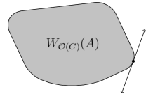
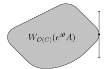
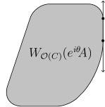
Since the orbit-closed -numerical range is convex when is selfadjoint, one natural way to analyze boundary points is to first rotate the operator and then take the real part, as in the diagram:
where we have used Proposition 3.7 to commute both and multiplication by with . In so doing one is able essentially to reduce the investigation of points on the boundary of the numerical range to the case when is selfadjoint. However, there are often technicalities that arise when there is a line segment on the boundary because, after rotation, there is more than one point on the boundary with maximal real part (see Figure 1). This rotation and real part technique goes all the way back to Kippenhahn in [28] (or the English translation [29, §3]), but appears elsewhere in the literature, such as [30].

We begin with a simple but rather important lemma concerning submajorization which will be essential in our analysis of the boundary. Effectively, it says that if then for any nonnegative decreasing sequence ; moreover, if and is strictly positive, then is block majorized by . The first part of the lemma, namely that implies , is a known result concerning submajorization (see, for example [31, 5.A.4.d]), but to the authors’ knowledge the remainder of the lemma has not appeared in the literature and we will make full use of these additional facts later on. To see the connection between the above formulation in terms of majorization and the actual statement of the lemma, consider .
Lemma 5.5.
Suppose that is a real-valued sequence and is a nonnegative decreasing sequence (even finite sequences are considered). If for every , , then
-
(i)
for every , ;
-
(ii)
if , then whenever with ,
and if, in addition, , then ; -
(iii)
if , then whenever .
Proof.
The proof is a simple application of summation by parts. Indeed, for any ,
Notice that by hypothesis are each nonnegative as are and for each . Therefore, as well, proving (i).
Moreover, if and for if , then . In addition, if , then , which establishes (ii).
Finally, notice that
Therefore, if the limit inferior on the left-hand side is zero, then we conclude whenever . ∎
The next proposition guarantees that the supremum of the orbit-closed -numerical range is attained whenever are positive and compact. This is our first sufficient condition for a point on the boundary to be included in .
Proposition 5.6.
Let be positive compact operators with trace-class. Then
and moreover the supremum is attained.
Proof.
Take any . Then since is a positive compact operator it is diagonalizable and so in some basis . Let be the diagonal of in this basis, which is necessarily nonnegative since is a positive operator. It is well-known that (e.g., see [17, Theorem 4.2]). Therefore, since is a nonincreasing nonnegative sequence, we may apply 5.5 to conclude for all ,
Taking the limit as , we find
Moreover, since the trace is trace-norm continuous, we have for any . Thus .
To show equality and thus that the supremum is attained, simply note that there is a (likely different) basis which diagonalizes since it is a positive compact operator, and in this basis (or if has finite rank). Then (or if has finite rank) by Proposition 3.1 and we obtain
Although the statement of the following theorem is restricted to the selfadjoint case, by the standard rotation argument mentioned at the beginning of this section, the next theorem provides a necessary and sufficient condition for a supporting line555recall that a supporting line for a convex set in the plane is a line such that and is entirely contained within one of the closed half-planes determined by . Notice that this latter condition ensures . of to contain at least one point of . Notice that if this supporting line intersects in exactly one point (in particular, if this point does not lie on a line segment on the boundary), then this theorem gives a necessary and sufficient condition for that point to lie in (cf. Figure 1).
We remark for the reader’s convenience a basic fact which will occur in the following theorem and repeatedly throughout the remainder of this paper. If and , then is a positive compact operator. Indeed, it clearly suffices to assume , and then simply notice that the spectral projections and are all finite for every .
Theorem 5.7.
Let be a positive trace-class operator and suppose is selfadjoint. Let . Then
Moreover, if denotes the spectral projection of onto the interval , then is attained if and only if . In fact, if attains the supremum, then .
Proof.
For and , since , by Proposition 3.7(iii), we may assume without loss of generality that .
The inequality is immediate because for any , since , we have by Proposition 3.7(i). Therefore
and taking the supremum over yields .
It remains to prove the reverse inequality and the claim concerning when the supremum is attained. We begin by proving the former.
Now, if , there is some such that by Proposition 3.1 (e.g., take ). Since are positive compact operators which are zero on , we may view them as operators acting on . By Proposition 5.6, there is some for which
Then setting we find that which we already established is at least . Moreover, notice that is attained in this case.
Now suppose . For , let . Since , we know that is a finite projection. But since , we must have that is infinite for every , and hence is infinite. Then consider a basis such that for , , and for which is an orthonormal set in . Define to be the diagonal operator for and for . Then by construction and since for , we find
Since was arbitrary, this proves , and thus we have equality.
Suppose attains the supremum, that is, . As we have just proved that , so then . Moreover, as and ,
| (5.1) | ||||
Since, , equality in (5.1) holds if and only if since the trace is faithful, if and only if .
Now because is the spectral projection of on the interval , we see that is strictly positive on (or ). Therefore, if and only if if and only if ( denotes the range projection of ) if and only if . This proves the claim about which attain the supremum.
Finally, if , then for any , and so by the above, does not attain the supremum. Since was arbitrary, the supremum cannot be attained in this case. ∎
The following example shows how the techniques developed thus far can be used to compute the orbit-closed -numerical range in certain circumstances.
Example 5.8.
Let denote the shift operator on either or . It is well known that the standard numerical range is , the open unit disk. Let with . We will show also.
Notice first that where is a rank- projection, so by Corollary 4.7, . Moreover, is unitarily equivalent to via the diagonal unitary . Therefore, since the orbit-closed -numerical range is unitarily invariant and using Proposition 3.7(iii), and so is radially symmetric. Because , we know , and therefore by Proposition 3.7(ii) and Theorem 5.7,
Consequently, by the radial symmetry and convexity (using Corollary 4.6) of it must contain the open unit disk. Therefore .
We note that must be dense in by Theorem 3.4, but it seems rather hard to conclude these sets are equal without convexity.
We now build towards Theorem 5.14 which provides a sufficient condition for to be closed for . We begin with a bootstrapping of a standard result by induction.
Lemma 5.9.
Given there is some such that whenever are each collections of mutually orthogonal projections with for each , then there is a unitary conjugating each pair such that .
Proof.
We proceed by induction on . The case when is standard, but a good reference is [32, II.3.3.4]. The argument is essentially this: set , then is invertible and is the desired unitary.
Now let and suppose the result holds for pairs of collections of mutually orthogonal projections of length at most . Let , then there is some corresponding to by the inductive hypothesis. Moreover, there is some corresponding to . Suppose that are each collections of mutually orthogonal projections with .
Then there is a unitary with conjugating to . Then also conjugates to a mutually orthogonal collection . Moreover,
Then let be a unitary conjugating to inside the Hilbert space such that . Then is a unitary on and . Finally, set and notice that conjugates to . Moreover,
By the induction, the proof is complete. ∎
Using Lemma 5.9 we now establish a sufficient condition for when certain points on the boundary can be obtained by elements of which are close in trace norm. This approximation result is a key step in the proof of Theorem 5.14.
Proposition 5.10.
Let and suppose that , where . Let denote the (possibly degenerate) line segment on consisting of the points with maximal real part.
Furthermore, suppose that there are arbitrarily small for which there is a point on its boundary whose supporting line intersects only at this point , and that as . Then given any , for sufficiently small there are some with and , and .
Consequently, contains points on the line segment arbitrarily close to .
Proof.
By translating, we may clearly suppose that . Define for each the selfadjoint operator .
Let . Since , there is some such that ; if , set . Let be the largest eigenvalues of with associated (mutually orthogonal) spectral projections for . Choose so that , which is possible since by hypothesis. Set and define and . We remark for future reference that when .
Notice that
where and that . Set
By the upper semicontinuity of the spectrum (and the essential spectrum), for all sufficiently small we can guarantee that and that is contained in the -neighborhood of .
By Lemma 5.9, there is some associated to . Then we may choose small enough so that both and is small enough [33, Theorem 3.4]666This result is actually much stronger than we need because it provides tight bounds on the required size of the norm . For our purposes, the result we need could be obtained by straightforward, albeit somewhat tedious, arguments using the continuous functional calculus. that if , then . Moreover, let . By Lemma 5.9 there is a unitary with conjugating to (i.e., ) for each .
Let be an orthonormal basis so that for (note: ), is an eigenvector of for the eigenvalue ; this is possible since by hypothesis , and also so . The eigenvectors are in the subspaces . More specifically, is a basis for . Consequently, is a basis for since conjugates to . Therefore, for , we have . So, these are eigenvectors for .
Now let be an orthonormal basis for which when (note: ); again, this is possible since , and because , so . By the previous paragraph we may select for . Let be the unitary which maps to for all . Notice that since and acts as the identity here since for .
Define to be the operator which is diagonal with respect to the basis such that for and for all other values of . Clearly by Proposition 3.1. Moreover, notice that
Then since maximizes , and because the supporting line for intersects the boundary only at that point, we must have .
Now define . Since maps the basis onto the basis , we see that is diagonal with respect to the basis . Moreover,
Since , this entails .
We now estimate the trace norm of . Since (or ) are diagonal with respect to the basis (or ) and therefore commute, we have
Additionally, since conjugates to , we know and so and . In addition, , and combining these we obtain
Combining these we find
Therefore,
Since and was arbitrary, we conclude that contains points on which are arbitrarily close to . ∎
We are almost ready to provide a sufficient condition for to be closed when and , but before we proceed we need two more technical results concerning majorization, spectral projections and operators which maximize for selfadjoint. Lemma 5.11 concerns, in essence, the properties of projections which maximize the -numerical range. Then Proposition 5.12 bootstraps Lemma 5.11 to conclude that a maximizer of the orbit-closed -numerical range has a certain block diagonal decomposition.
Lemma 5.11.
Let be a positive compact operator and a rank- projection. If
and , then and . Consequently, commutes with .
Proof.
In the case when , then and . Therefore . Since the trace is faithful, this implies , and therefore that . Therefore .
Therefore we may suppose . Let be the distinct eigenvalues of greater than or equal to , and let for be the associated spectral projections. Then , and . Let be the largest eigenvalue of less than . Set , so that . For convenience of notation we set . We remark that .
Notice that for , and that
Therefore, we have majorization of the finite sequences
| (5.2) |
Consider the difference of these sequences which, since , has the form
Then because and for , and since has nonnegative partial sums,
| by Lemma 5.5 with (5.2), | ||||
where . By hypothesis the first and last expressions in the above chain are equal, and therefore we must have equality throughout.
Since from the previous display , and because the are distinct and positive, Lemma 5.5 guarantees for all . Therefore, and hence . Similarly, for , , and thus , so we may write for some projection . Finally, the projection .
Notice that commutes with any subprojection of (because is scalar relative to this subspace), hence commutes with . Since also commutes with (because it is a spectral projection), it must commute with as well. ∎
The next proposition guarantees a kind of block diagonal decomposition for those which maximize for selfadjoint . This proposition is essential in proving: Theorem 5.14, which establishes a sufficient condition for to be closed for some ; Theorem 6.2, which characterizes the behavior of the orbit-closed -numerical range under direct sums; and Theorem 6.8, which establishes an analogue for the orbit-closed -numerical range of when is normal.
Proposition 5.12.
Suppose that is a positive trace-class operator and is selfadjoint with . Let denote the distinct elements of greater than listed in decreasing order, and including when this list is finite.
If is a maximizer of , that is, if , then commutes with each of the projections for . Moreover, for , the compression of to is unitarily equivalent to where and . Furthermore, if , then the compression of to lies in , where this sequence is infinite if .
Proof.
By translating and applying Proposition 3.7 and Theorem 5.7 we may assume without loss of generality that . Then are the distinct terms in the sequence listed in decreasing order, and for , the multiplicity of in this sequence is exactly . Set .
Let be an orthonormal basis where is a basis for and for each , the collection is a basis for . Then let be the diagonal of relative to this basis. We have . Therefore
Then by Lemma 5.5 we obtain for each , . Therefore, for each , we find
Then by Lemma 5.11, commutes with ; moreover, if denote the compression of to , then .
Consequently, if we consider to be the compression of to , then lies in . Therefore, we may again apply Lemma 5.11 to conclude that (and hence also ) commutes with . Moreover, if denotes the compression of to , then .
Continuing this procedure, by induction on we obtain for each that commutes with , and that the compression of to is a matrix of size with .
If , then the proof is already complete. If, on the other hand, , then and we must consider , which is the compression of to . From the above, we know that . However, and . By Theorem 5.7, since is a maximizer of , we must have that , and therefore the compression of to lies in . ∎
Using Proposition 5.12, it is possible to give a condition under which , or even , is attained when and .
Remark 5.13.
Suppose that are positive compact operators with infinite rank and that is trace-class. Every for which satisfies . Indeed, by Proposition 5.12, for the projections for , the operator commutes with each and the compression of to lies in . Consequently, is strictly positive on and must be zero on the complement. Notice that is the projection onto . Thus .
Therefore, there is an for which if and only if777if , then , and relative to the proper basis so by Proposition 5.6. .
We conclude this section by using Theorem 5.7 and Propositions 5.10 and 5.12 to establish in Theorem 5.14 a sufficient condition for to be closed.
Theorem 5.14.
Let be a positive trace-class operator and let . Then is closed if for every , , where .
Proof.
Suppose that the rank condition holds for every angle . Let . There are two possibilities.
Case 1. There is a supporting line for which intersects only at .
After applying a suitable rotation, we may assume that and that the supporting line is vertical, so that is the unique point of with maximal real part. Since , Theorem 5.7 guarantees that is attained, and by uniqueness this must be achieved by .
Case 2. The only supporting line for containing intersects in a line segment .
After applying a suitable rotation, we may assume that , so the line segment is vertical and has maximal real part. Moreover, by translating we may further assume . In order to prove that , it suffices to show that since this set is convex by Corollary 4.6.
We consider only , as the analysis for is identical. Then there are two possibilities. The first is that itself has a (different) supporting line for which intersects only at , in which case by Case 1; this happens precisely when is a corner of .
The alternative is that there are no other supporting lines passing through . This implies that for any , the supporting line of with slope intersects the boundary at a point distinct from . Now, we claim that there are arbitrarily small such that this line intersects at a unique point , which must be in by Case 1. Indeed, if not, for each sufficiently small angle , would contain a nondegenerate line segment with slope , but this would imply that has infinite length (since the sum of uncountably many positive numbers is necessarily infinite), which would violate the fact that is rectifiable — a well-known consequence of being a bounded convex curve. Moreover, it is clear that as for whichever positive the point is defined.
Thus the situation satisfies the hypotheses of Proposition 5.10, and so we are guaranteed that contains points on the line segment arbitrarily close to . So consider a sequence of points in converging to . Then there are with , and hence . We may therefore apply Proposition 5.12 to obtain finite projections such that the compression of to lies in and moreover commutes with each . If we set , then since , we see that . So is block diagonal with respect to the blocks , and . Note, the projections for these blocks are independent of .
Now, by the Schur–Horn theorem ([34, 35], but see [18, Theorem 1.1] for a concise, self-contained statement), there are block unitaries for which . Moreover, we can select . It is important to note that for each , is a finite matrix of size .
We now apply the standard recursive subsequence technique to obtain a subsequence of the unitaries with desirable properties. More specifically, by compactness of the unitary group in finite dimensions, there is a subsequence such that converges to some unitary matrix (of size ). Then for we inductively construct a subsequence of for which converges to some unitary matrix . Then consider the subsequence of the original sequence given by . Define and . Note that converges entrywise to , but not necessarily in any operator topology.
We claim that converges in trace-norm to . Indeed, let and since is trace-class, there is some such that . Set , which is a finite projection that commutes with because each does. Moreover, because converges entrywise to and is a finite projection, converges to in trace norm (or any other norm topology since all norms on a finite dimensional space are equivalent). Therefore there is some such that for all , . Thus we obtain
In addition,
Therefore, combining the above displays yields
Thus . Since , we find .
Finally, a symmetric argument applies to , and hence . Because is convex by Corollary 4.6, , thereby completing the proof. ∎
The following example shows that although the hypothesis of Theorem 5.14 is not a necessary condition for to be closed, it is in some sense sharp.
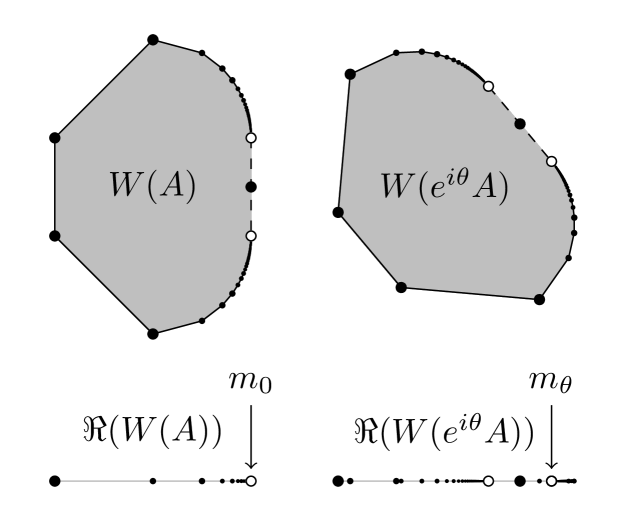
Example 5.15.
This example shows that if the rank condition in Theorem 5.14 fails for even a single angle , it is possible for not to be closed, even if contains at least one boundary point for every angle . In fact, this example even uses the usual numerical range and a diagonalizable operator .
Consider the diagonalizable operator whose eigenvalues are and for all , each with multiplicity one. Then the line segment lies on the boundary , but , although nonempty, contains only a single point. Moreover, , but for any . See Figure 2 for a diagram of this situation.
The part of the proof which breaks down because is in the approximation result Proposition 5.10. In particular, there aren’t enough (any) spectral projections corresponding to nonzero eigenvalues of .
Of course, if we modify to have the eigenvalues as well, then becomes closed even though we still have . Therefore the sufficient condition given in Theorem 5.14 is not necessary. There are even simpler examples: the orbit-closed -numerical range of a scalar is closed (a singleton), but for all .
6 Compact normal operators and the -spectrum
It is a standard result in linear algebra that for a normal matrix the standard numerical range satisfies , which is an immediate consequence of the elementary (finite or infinite dimensional) fact that . Of course, there are many ways to extend or generalize this result.
One can extend it to the infinite dimensional setting in two ways. For normal , there is the folklore result . However, restricting to normal , de Barra, Giles and Sims proved [25, Theorem 2].
The other option is to generalize the matrix result to other numerical ranges, such as the -numerical range or the -numerical range. In this case, one needs a substitute for the spectrum which is somehow relativized to the matrix . For normal, Marcus [12] introduced a substitute, now referred to as the -spectrum and denoted888 This notation is common in the later literature, but Marcus actually used the notation to refer to the convex hull of the -spectrum, and he called this the -eigenpolygon. , consisting of the sums of products of the eigenvalues of . There he proved that if is also normal, then .
Dirr and vom Ende extended the notion of -spectrum to the infinite dimensional setting with and [13, Definition 3.2], where they also managed to prove [13, Theorem 3.4, Corollary 3.1] that if are both normal, then
| (6.1) |
Moreover, if is normal and is upper triangular, or vice versa, [13, Theorem 3.5].
While Dirr and vom Ende’s results are impressive, because of the hypothesis and de Barra, Giles and Sims result , one might hope for the chance to remove the closures from in (6.1). In this section, for , we do precisely that for the orbit-closed -numerical range and the -spectrum (see Definition 6.3), which is a (not necessarily closed) slight modification of the -spectrum defined by Dirr and vom Ende (see Remark 6.4). In particular, Theorem 6.8 says that if and is normal, then . Along the way, with Theorem 6.2 we characterize the behavior of the orbit-closed -numerical range under direct sums, thereby generalizing the finite rank result [26, Result (4.4)].
Lemma 6.1.
Let be a positive trace-class operator, an arbitrary projection, and suppose is selfadjoint, where act on , respectively. Then
and if either supremum is attained, then they both are.
Proof.
The inequality is trivial since the latter set is a subset of the former. We split the remainder of the proof into cases. By translating, we may assume .
Case 1. The supremum is attained.
We must produce an with . By Theorem 5.7 we are guaranteed that . Let denote the distinct nonnegative eigenvalues of listed in decreasing order and including zero if and only if this set is finite. Then let be the associated spectral projections. Set .
Since commutes with it commutes with each , so we may write which is a sum of orthogonal projections. Let and for set . Note that if , then which may be either a finite or infinite projection, so may be either finite or infinite. Then for each , we may select the finite matrix acting on and respecting the decomposition , so that , where is a matrix of size and is a matrix of size . The situation for is similar, except that the matrices involved might be infinite. That is, we can consider the operator acting on the (possibly infinite dimensional) space . Set acting on and , respectively.
Setting and , we claim that is the desired operator. Indeed, notice that is either infinite or equal to , which is in either case greater than or equal to . Therefore, the operators have exhausted all the nonzero values of the sequence (i.e., if ) and hence . Moreover, since whenever , we find
Now , and so we have
where the last equality is due to Theorem 5.7.
Case 2. The supremum is not attained.
In this case, by Theorem 5.7 , and so this projection is finite. Since , the projection must be infinite for any , and since is a spectral projection for , it commutes with because does. Therefore is a sum of projections and at least one of these projections must be infinite.
Let . Since , by Case 1 we know that there is some for which
where the third equality follows because for . Moreover, by Theorem 5.7 .
Now let be the operator given by on the subspace (or , whichever is infinite) and zero on the orthogonal complement in . Then commutes with (so it has a direct sum decomposition), and
Since is arbitrary, this proves
and therefore we must have equality. Finally, because and is not attained, the equality of the suprema guarantees that is not attained either. ∎
Of course, by replacing with in Lemma 6.1 one immediately obtains the exact same result with the suprema replaced by infima. Moreover, the finite dimensional counterpart of Lemma 6.1 is a known result (see [9, Result (4.2)]), and in that case the suprema are always attained by compactness. We will make use of both of these facts in order to establish the following theorem.
Theorem 6.2.
Let be a positive trace-class operator, an arbitrary projection, and suppose , where act on , respectively. Then
Proof.
The case when has finite rank appears in [26, Result (4.4)], so we will prove the result when has infinite rank.
One inclusion is immediate. Indeed, given with , it is clear that . Therefore,
Since was arbitrary, as were and , we obtain
By Corollary 4.6, is convex and so contains the convex hull of this union.
We now prove the other inclusion. For convenience, we replace by since . For set and notice that . Therefore in the Hausdorff pseudometric by Theorem 3.5.
For any , and let denote the projection onto the span of the eigenvectors associated to . Note that commutes with and therefore we can naturally obtain via Doing so ensures that for . Conversely, given , both are finite rank and positive, therefore at least one of them has an infinite dimensional reducing subspace because one of them must act on an infinite dimensional space. Then adding acting on that subspace yields an operator which again satisfies for .
Hence, by Theorem 3.5 the Hausdorff distance between these orbit-closed -numerical ranges satisfies
Therefore, the corresponding unions converge in Hausdorff pseudometric
Additionally, their convex hulls converge in the Hausdorff pseudometric as well. Since the theorem is valid when the trace-class operator is finite rank [26, Result (4.4)] we have the convergence
| same closure |
Since and are convex and have the same closure, they must have the same interior. Hence it suffices to prove any boundary point of lies in the above convex hull.
Now suppose lies on the boundary. By the usual rotation and translation technique, we may assume has maximal real part and . Since , we may apply Proposition 5.12. Let denote the distinct nonnegative eigenvalues of listed in decreasing order, and including zero if and only if . Let be the associated spectral projections and set . Let and for , . Then Proposition 5.12 guarantees that commutes with each , so that where acts on . Moreover, and for , , where . If , then where .
Let the reader take note that any operator with properties of listed in the previous paragraph (block diagonal with respect to with blocks in the associated orbits) has the property that . We will use this property shortly.
Let denote the compression of to . In general, will not be block diagonal with respect to these blocks because is not necessarily normal so may not commute with . However, commutes with , and therefore with and , which implies that it also commutes with each spectral projection . Therefore, we may write each as a sum of projections, and also , where act on and , respectively.
Now,
| (6.2) |
where we have omitted the term from the sum since . For each , the operators act on the finite dimensional space , and so the supremum is attained. Moreover, because , by Lemma 6.1 (or rather, its finite dimensional counterpart) there exists such that . If , then Lemma 6.1 still allows us to obtain such that regardless of whether or not is attained. Set . Then set and and . As previously remarked, satisfies the same decomposition property as , and therefore . Moreover, .
Notice that
Therefore, a symmetric argument to the one given in the previous paragraph allows us to produce a such that and . This proves that
as desired. ∎
In [13], Dirr and vom Ende introduced an analogue of the -spectrum for trace-class when is compact, which they also denoted . We will also need a notion of the -spectrum of a compact operator , but ours will differ slightly from the one given by Dirr and vom Ende, and for this reason we will instead use the notation and refer to it as the -spectrum.
As in [13], we must invoke the concept of the modified eigenvalue sequence of a compact operator . This is the sequence obtain by mixing many zeros into the usual eigenvalue sequence . For the purposes of -spectrum the order of these eigenvalues does not matter.
Definition 6.3.
Let be a trace-class operator of (possibly infinite) rank , and let . The -spectrum of is the collection
One should think of the -spectrum as an -relativized analogue of the point spectrum .
This definition of -spectrum differs from the definition of -spectrum given in [13] only in that we allow to be injective instead of a permutation, and that we use the standard eigenvalue sequence of instead of the modified eigenvalue sequence.
Remark 6.4.
The terminology -spectrum and notation is not haphazard, but alludes to the following relationship between the -spectrum, the -spectrum and the point spectrum. For a normal operator and , by Proposition 3.1
So, in essence, the -spectrum is just a version of the -spectrum where the size of the kernel of can vary, at least when is normal.
Moreover, if is finite rank, then , and if is a rank- projection, then .
It is a trivial fact that the point spectrum of an operator is contained in the numerical range , and by convexity . The following proposition establishes an analogous fact for the -spectrum and the orbit-closed -numerical range.
Proposition 6.5.
If is normal and is upper triangular relative to some orthonormal basis, then . If, in addition, is selfadjoint, then the inclusion also holds.
Proof.
Suppose that is upper triangular relative to an orthonormal basis for . Then it is well known that the diagonal entries of are precisely the (suitably permuted) modified eigenvalue sequence . Indeed, the sequence of subspaces
forms a triangularizing chain for , and so the nonzero diagonal entries are precisely the eigenvalues by Ringrose’s Theorem, and they are repeated according to algebraic multiplicity (see [36, Theorems 7.2.3 and 7.2.9]).
Then take any injective and define a sequence by
Then since is normal, by Proposition 3.1 . Moreover,
Since was arbitrary, .
Finally, if is selfadjoint, then by Corollary 4.6, is convex and therefore . ∎
Before we prove our last main theorem in this section (Theorem 6.8), which says that when is normal and , we need lemmas corresponding to two special cases: selfadjoint, and normal with finite spectrum.
Lemma 6.6.
If and , then .
Proof.
Since is diagonalizable, by Proposition 6.5 we only need to prove the inclusion .
Notice that is an interval since it is convex and contained in . We will prove that when is attained then it is an element of , and when the supremum is not attained, contains elements arbitrarily close to . Of course, symmetric arguments apply to the infimum, thereby establishing the desired equality .
By Theorem 5.7 and Proposition 5.6 we know that
and that this supremum is attained if and only if . Moreover, since for , is an eigenvalue for , when the inequality holds, we obtain
In the case when is not attained, we know that (so ), and therefore is a finite projection. Since , for every , the projection is infinite. Therefore has infinitely many arbitrarily small negative eigenvalues. Let be an injective function such that for and for , . Multiplying this inequality by and summing over yields . Therefore,
Therefore contains elements which are arbitrarily close to .
As remarked at the beginning of the proof, symmetric arguments hold for , and therefore . ∎
Lemma 6.7.
If is normal with finite spectrum and , then .
Proof.
Let listed in order of decreasing modulus, and let be the corresponding spectral projections. Of course, , so after relabeling we may assume , and therefore is the only infinite projection among the list since .
Now , by Theorem 6.2, every element of is a convex combination of terms of the form where and acts on . We claim that any such term lies in . Indeed, suppose that for , is a basis for which diagonalizes , and that is a basis for which diagonalizes .
Since is diagonal relative to this orthonormal basis , the nonzero terms of its diagonal sequence must consist precisely of the nonzero terms of . Moreover, relative to this basis, is already diagonalized and its diagonal is precisely . Let be an injective function such that . Then we find
Since any element of is a convex combination of such terms, we obtain the inclusion , and equality follows from Proposition 6.5. ∎
Theorem 6.8.
If is a positive trace-class operator and is compact normal, then the orbit-closed -numerical range and the convex hull of the -spectrum coincide. That is,
Proof.
Since a normal operator is diagonalizable, by Proposition 6.5 we only need to prove the inclusion .
Consider a basis diagonalizing , so that . Then for we define the finite rank operators and notice . Therefore in the Hausdorff pseudometric by Theorem 3.5.
Now is a normal compact operator with finite spectrum, so by 6.7 we obtain .
We now prove that . Let , and choose such that for all , . Let be any injective function. Then
Consequently, , so . Moreover, this implies converges to in the Hausdorff pseudometric as well. Thus
and hence .
By the above, it suffices to prove that every element of the boundary of is also an element of . The argument is very similar to the one in the proof of Theorem 6.2, except we apply Lemma 6.6 in place of Lemma 6.1.
Suppose that lies on the boundary. By rotating, we may suppose that . Then by Proposition 5.12 we get spectral projections associated to the distinct nonnegative eigenvalues of , including zero if and only if . We set and , and . In addition, commutes with each and if denotes the compression of to , then . Moreover, and for we have where . If , then where .
Since is normal, it is clear that commute, and therefore commutes with each , and so commutes with too. Let be the compression of to , so . Now for each , by Lemma 6.6 we know that there are elements such that . Moreover, since , then . Notice that , hence . Summing over , we obtain
Finally, , and therefore we obtain . ∎
7 Convexity of the -numerical range.
In their paper [13], Dirr and vom Ende asked whether the -numerical range is convex when is normal with collinear eigenvalues. We will now show that when is diagonalizable and is positive and has either trivial or infinite dimensional kernel, then this is indeed the case (see Corollary 7.3). We make no claim that these circumstances are exhaustive, but we are limited by the proof technique and the underlying results. Nevertheless, we felt that a partial answer to the question of the convexity of would contribute some value.
Let denote the canonical trace-preserving conditional expectation onto a diagonal masa . In other words, is the operation of “taking the main diagonal.” When applied to the unitary orbit of an operator , there is a natural bijection between and the set of all diagonal sequences of as the orthonormal basis giving rise to the matrix representation of varies. The study of diagonal of operators has a rich history in the literature. For a survey, see [37].
The following999In [18], this is stated in terms of the so-called partial isometry orbit, , but [19, Proposition 2.1.12] guarantees that for . gives a complete characterization of diagonals of compact operators modulo the dimension of the kernel.
Proposition 7.1 ([18, Proposition 6.4]).
For a positive compact operator ,
Since the set is readily seen to be convex, Proposition 7.1 can be used to give a one-line proof that is convex whenever is diagonalizable, thereby providing yet another proof of Theorem 4.5 in this restricted setting. Indeed, suppose and let and suppose . Then there is some for which , and therefore
Since the conditional expectation is trace-preserving, .
It turns out that there are certain circumstances under which has been characterized, namely when is either trivial [18, Proposition 6.6] or infinite dimensional [38, Corollary 3.5]. In both cases, the characterization is still linked to majorization but the details of the definitions are a bit too technical for our present purposes. Nevertheless, it is known that is convex if is trivial [18, Corollary 6.7] or infinite dimensional101010In the case when is nontrivial but finite dimensional, the first author has conjectured a characterization of and has established that this conjectured set is convex. See [38, Conjecture 3.6, Lemma 4.2] for details. [38, Corollary 4.3].
Proposition 7.2 ([18, Corollary 6.7],[38, Corollary 4.3]).
Let be a positive compact operator. If is either trivial or infinite dimensional, then is convex.
This immediately yields the following corollary concerning the convexity of .
Corollary 7.3.
Let be a positive trace-class operator and suppose that is either trivial or infinite dimensional. For any diagonalizable operator , is convex.
Proof.
Suppose is diagonalizable. Then after conjugating by a suitable unitary, which we can absorb into , we may assume . Let and suppose . Then by Proposition 7.2 there is some for which , and therefore
Then since the conditional expectation is trace-preserving. ∎
References
- [1] Toeplitz O. Das algebraische Analogon zu einem Satze von Fejér. Math Z. 1918;2(1-2):187–197.
- [2] Hausdorff F. Der Wertvorrat einer Bilinearform. Math Z. 1919;3(1):314–316.
- [3] Davis C. The Toeplitz-Hausdorff theorem explained. Canad Math Bull. 1971;14:245–246.
- [4] Halmos PR. Numerical ranges and normal dilations. Acta Sci Math. 1964;25:1–5.
- [5] Berger CA. Normal dilations [dissertation]. Cornell University; 1963. Advisor: Morris Schreiber; Available from: https://hdl.handle.net/2027/coo.31924001140247.
- [6] Fillmore PA, Williams JP. Some convexity theorems for matrices. Glasg Math J. 1971;12:110–117.
- [7] Westwick R. A theorem on numerical range. Linear Multilinear Algebra. 1975;2:311–315.
- [8] Goldberg M, Straus EG. Elementary inclusion relations for generalized numerical ranges. Linear Algebra Appl. 1977;18:1–24.
- [9] Li CK. -numerical ranges and -numerical radii. Linear Multilinear Algebra. 1994;37(1-3):51–82.
- [10] Au-Yeung YH, Tsing NK. A conjecture of Marcus on the generalized numerical range. Linear Multilinear Algebra. 1983;14:235–239.
- [11] Cheung WS, Tsing NK. The -numerical range of matrices is star-shaped. Linear Multilinear Algebra. 1996;41(3):245–250.
- [12] Marcus M. Some combinatorial aspects of numerical range. Ann NY Acad Sci. 1979;319(1):368–376.
- [13] Dirr G, vom Ende F. The -numerical range in infinite dimensions. Linear Multilinear Algebra. 2020;68(4):652–678.
- [14] Dykema K, Skoufranis P. Numerical ranges in II1 factors. Proc Edinb Math Soc, II Ser. 2017;61(1):31–55.
- [15] Poon YT. Another proof of a result of Westwick. Linear Multilinear Algebra. 1980;9:35–37.
- [16] Birkhoff G. Three observations on linear algebra. Univ Nac Tucumán Revista A. 1946;5:147–151.
- [17] Arveson W, Kadison RV. Diagonals of self-adjoint operators. In: Han D, Jorgensen PE, Larson DR, editors. Operator theory, operator algebras, and applications. (Contemp. Math.; Vol. 414). Amer. Math. Soc., Providence, RI; 2006. p. 247–263.
- [18] Kaftal V, Weiss G. An infinite dimensional Schur–Horn Theorem and majorization theory. J Funct Anal. 2010;259(12):3115–3162. Available from: http://www.sciencedirect.com/science/article/pii/S0022123610003563.
- [19] Loreaux J. Diagonals of operators [dissertation]. University of Cincinnati; 2016.
- [20] Gellar R, Page L. Limits of unitarily equivalent normal operators. Duke Math J. 1974;41:319–322.
- [21] Voiculescu D. A non-commutative Weyl-von Neumann theorem. Rev Roumaine Math Pures Appl. 1976;21(1):97–113.
- [22] Hiai F, Nakamura Y. Closed convex hulls of unitary orbits in von Neumann algebras. Trans Am Math Soc. 1991;323(1):1–38.
- [23] Chu CH. A note on scattered C*-algebras and the Radon-Nikodym property. J Lond Math Soc, II Ser. 1981;24:533–536.
- [24] Phelps RR. Dentability and extreme points in Banach spaces. J Funct Anal. 1974;17:78–90.
- [25] de Barra G, Giles JR, Sims B. On the numerical range of compact operators on Hilbert spaces. J Lond Math Soc, II Ser. 1972;5:704–706.
- [26] Li CK, Poon YT. Some results on the -numerical range. In: Five decades as a mathematician and educator. On the 80th birthday of Professor Yung-Chow Wong. Singapore: World Scientific; 1995. p. 247–258.
- [27] Fan P, Fong CK. Which operators are the self-commutators of compact operators? Proc Amer Math Soc. 1980;80:58–60.
- [28] Kippenhahn R. Über den Wertevorrat einer Matrix. Math Nachr. 1951;6:193–228.
- [29] Kippenhahn R. Über den Wertevorrat einer Matrix. Linear Multilinear Algebra. 2008;56(1-2):185–225.
- [30] Johnson CR. Numerical determination of the field of values of a general complex matrix. SIAM J Numer Anal. 1978;15:595–602.
- [31] Marshall AW, Olkin I, Arnold BC. Inequalities: theory of majorization and its applications. 2nd edition. 2nd ed. New York, NY: Springer; 2011.
- [32] Blackadar B. Operator algebras. Theory of -algebras and von Neumann algebras. Berlin: Springer; 2006.
- [33] Makarov KA, Seelmann A. The length metric on the set of orthogonal projections and new estimates in the subspace perturbation problem. J Reine Angew Math. 2015;708:1–15.
- [34] Schur I. Über eine klasse von mittelbildungen mit anwendungen auf der determinantentheorie. Sitzungsber Berliner Mat Ges. 1923;22:9–29.
- [35] Horn A. Doubly stochastic matrices and the diagonal of a rotation matrix. Amer J Math. 1954;76:620–630.
- [36] Radjavi H, Rosenthal P. Simultaneous triangularization. New York, NY: Springer; 2000.
- [37] Loreaux J, Weiss G. On diagonals of operators: selfadjoint, normal and other classes. In: Operator Theory: Themes and Variations — Conference Proceedings, Timişoara, July 2–6, 2018; 2020. p. 193–214.
- [38] Loreaux J, Weiss G. Majorization and a Schur–Horn Theorem for positive compact operators, the nonzero kernel case. J Funct Anal. 2015 February;268(3):703–731. Available from: http://www.sciencedirect.com/science/article/pii/S0022123614004625.