Frustrated bearings

Abstract

In a bearing state, touching spheres (disks in two dimensions) roll on each other without slip. Here we frustrate a system of touching spheres by imposing two different bearing states on opposite sides and search for the configurations of lowest energy dissipation. If the dissipation between contacts of spheres is viscous (with random damping constants), the angular momentum continuously changes from one bearing state to the other. For Coulomb friction (with random friction coefficients) in two dimensions, a sharp line separates the two bearing states and we show that this line corresponds to the minimum cut. Astonishingly however, in three dimensions, intermediate bearing domains, that are not synchronized with either side, are energetically more favorable than the minimum-cut surface. Instead of a sharp cut, the steady state displays a fragmented structure. This novel type of state of minimum dissipation is characterized by a spanning network of slipless contacts that reaches every sphere. Such a situation becomes possible because in three dimensions bearing states have four degrees of freedom.

A bearing is a set of spheres (discs in 2d) that, with the position of their centers fixed, roll on each other without any slip at their contacts Herrmann1990 ; Manna1991 ; Baram2004 , transferring torque without dissipation. A sufficient condition to achieve a bearing state is to ensure that the graph of contacting spheres is bipartite, that is, all loops in the graph have an even number of spheres Baram2004 ; Stager2016 . In two dimensions, the tangential velocities $v$ at all contacts must be identical, so that the bearing state is uniquely defined by $v$. In three dimensions, other types of bearing states can be identified Stager2016 .

The concept of bearings plays an important role on the dynamics of dense packings of particles Alonso-Marroquin2006 ; Ayer1965 ; Jodrey1985 ; Yu1988 ; Bessis1990 ; Konakawa1990 ; Standish1991 ; Roux1993 ; Yu1993 ; Anishchik1995 ; Elliott2002 ; Baram2004 ; Ciamarra2006 ; Astrom2008 ; Halsey2009 ; Sobolev2010 ; Reis2012 ; Martin2015 ; Stager2016 ; Peshkov2019 . Bearings obtained by construction that completely fill space Manna1991a ; Oron2000 ; Baram2004a ; Baram2005 ; Kranz2015 ; Stager2018 can support large pressures while allowing for sliding movement. Moreover, it was shown that the synchronization process necessary to reach a global bearing state can be substantially enhanced by adjusting the inertial contribution of individual rotors Araujo2013 . When the particles move, inducing a complex and changeable force network Tkachenko1999 , as it is the case in shear bands, bearing states form spontaneously Astrom2000 ; Latzel2003 . Due to these properties, it was suggested Herrmann1990 ; Roux1993 ; Astrom2000 that such bearing states may explain the existence of “seismic gaps”, namely, regions in tectonic faults that should be moving, but where no earthquake activity has been detected for a long time Lomnitz1982 ; Kagan1991 .

While the transfer of momentum through disordered systems has been studied extensively, much less is known about the transfer of torque. In particular, when contacts dissipate due to Coulomb friction instead of viscous forces, systems can get stuck in particular configurations. Here we investigate a system of touching rotors subjected to frustrating boundary conditions, that is, systems where one side is forced to be in one bearing state, while on the other side another bearing state is imposed. Between these two bearing states there must be slipping contacts with random friction coefficients where energy is dissipated. Following its natural dynamics, a bearing system will settle to one configuration, albeit frustrated, of minimum energy loss.

In our computational model, we place touching spheres (disks in 2d) on a regular grid in such a way that their positions are fixed but they can rotate. At every contact a tangential friction force $F_{t(ij)}$ acts on the pair of particles $i$ and $j$. We consider two cases, namely, either this force is viscous,

$$F_{t(ij)}=\eta_{ij}v_{r(ij)},$$ (1)

where $\eta$ is a damping coefficient, and $\vec{v}_{r}$ is the relative slipping velocity

$$\vec{v}_{r(ij)}=\vec{\omega}_{j}\times\vec{r}_{ji}-\vec{\omega}_{i}\times\vec{r}_{ij},$$ (2)

or Coulomb-like

$$F_{t(ij)}=\left\{\begin{matrix}F_{s(ij)}&\text{if }v_{r(ij)}\neq 0\\ \mu_{ij}F_{n}&\text{if }v_{r(ij)}=0,\end{matrix}\right.$$ (3)

where $F_{s}$ and $F_{n}$ are the static friction and the normal force on the contact, respectively. In order to find the stationary state, we use two different numerical techniques. On one hand, we find the configuration that minimizes the dissipation power $P$, which is defined as,

$$P=\frac{1}{2}\sum_{i}^{N}\sum_{j}^{\{i\}}\vec{F}_{t(ij)}\cdot\vec{v}_{r(ij)},$$ (4)

where the sum in $j$ goes over the set $\{i\}$ of disks that are in contact with disk $i$. We use about $10^{6}$ iterations steps of gradient descent Ruder2016 in order to find the state that minimizes $P=P(\vec{\omega}_{1},\vec{\omega}_{2},\ldots,\vec{\omega}_{n})$. For a viscous friction force, the components of $\nabla_{\vec{\omega}_{1},\vec{\omega}_{2},\ldots,\vec{\omega}_{n}}P$ can be written as,

$$\frac{\partial P}{\partial\omega_{i,k}}=2\sum_{j}\eta_{ij}(\vec{\omega}_{i}\times\vec{r}_{ij}-\vec{\omega}_{j}\times\vec{r}_{ji})\cdot(\hat{k}\times\vec{r}_{ij}),$$ (5)

while for a Coulomb-like friction force they become,

$$\frac{\partial P}{\partial\omega_{i,k}}=F_{n}\sum_{j}\mu_{ij}\frac{(\vec{\omega}_{i}\times\vec{r}_{ij}-\vec{\omega}_{j}\times\vec{r}_{ji})}{\left\|\vec{\omega}_{i}\times\vec{r}_{ij}-\vec{\omega}_{j}\times\vec{r}_{ji}\right\|}\cdot(\hat{k}\times\vec{r}_{ij}),$$ (6)

where the sum in $j$ goes just over the slipping contacts of sphere $i$. In a second approach, we use a Cundall-Strack scheme Cundall1979 ; Brendel1998 in order to obtain an approximation for the friction force,

$$\vec{F}_{t}=\left\{\begin{matrix}\mu_{k}F_{n}(\vec{v}_{r}/||\vec{v}_{r}||)&\hskip 56.9055pt&\text{if }||\vec{F}_{s}^{*}||>\mu_{s}||\vec{F}_{n}||\\ \vec{F}_{s}^{*}&\hskip 56.9055pt&\text{otherwise}.\end{matrix}\right.$$ (7)

Here, $\mu_{s}$ and $\mu_{k}$ are the static and the dynamic friction coefficients, respectively, and $\vec{F}_{s}^{*}$ mimics the static friction force,

$$\vec{F}_{s}^{*}=-K_{t}\vec{\delta}-A_{t}\vec{v}_{r}.$$ (8)

Figure 1: Stationary configurations for (a) viscous damping and (b) Coulomb friction in the contacts of a packing of disks whose centers are the vertices of a square lattice of size $10\times 10$. The boxes indicate the positions of the imposed boundary conditions. Disks at the bottom are constrained to remain static, $\omega_{B}=0$, while those at the top rotate with a given angular velocity, $\omega_{T}>0$, as a fixed bearing. Except for the bottom and top rows, all angular velocities of the disks were initially set randomly. Regardless of the initial condition, given the disorder in the friction coefficients, the system always evolves to the same stationary configuration. The color bar corresponds to the ratio between the moduli of the angular velocities $\omega$ of the spheres and the imposed modulus of the angular velocities at the top boundary $\omega_{T}$. There is no slipping or dissipation in the contacts between disks of the same color. In (b), the interface between the two bearing states is identical to the minimum cut corresponding to the friction coefficients of the contacts. This equivalence is due to the fact that dissipation occurs only at the interface. Simulations with 1000 different sets of disordered friction coefficients showed that the boundary corresponds to the minimum cut in 983 cases. The remaining cases corresponded to systems with two distinct minimal cuts with values very close to each other. In such cases, the final state can present two boundaries at these cuts.

Static friction is idealized as an imaginary tangential spring used to keep the contact point slipless, where $\vec{\delta}$ is the elongation of this spring, $K_{t}$ its stiffness, and the constant $A_{t}$ damps any oscillation in the synchronized contacts. For simplicity, we use a viscous damping force proportional to the relative tangential velocity at the contact point $\vec{v}_{r}$. In our simulations $K=10^{5}$, $A=10^{3}$ and $F_{n}=50$ for discs (spheres in 3D) of radii 0.5. These values ensure that for very small $\delta=10^{-4}$ the threshold of dynamic friction is reached. We tested different values of $F_{n}$ and greater values of $K$ and $A$, but no significant differences were observed.

For the elongation $\vec{\delta}$, we use the following representation,

$$\vec{\delta}=\left\{\begin{matrix}-(\mu_{k}||\vec{F}_{n}||/K_{t})\vec{F}_{s}^{*}&\text{if }||\vec{F}_{s}^{*}||>F^{*}_{s\;\text{max}}=\mu_{s}||\vec{F}_{n}||\\ \displaystyle\vec{\delta}(t^{\prime})+\int_{t^{\prime}}^{t}{\vec{v}_{r}}{dt^{\prime\prime}}&\text{otherwise},\end{matrix}\right.$$ (9)

where $t^{\prime}$ is the time when $\vec{v}_{r}$ changes for the first time after $F_{s}^{*}$ reaches the threshold $F^{*}_{s\;\text{max}}$ Cundall1979 ; Brendel1998 . We use Gear’s algorithm Gear1967 ; Allen1987 to integrate the equations of motion,

$$I\frac{\partial^{2}\vec{\omega}_{i}}{\partial t^{2}}=\sum_{j}^{\{i\}}\vec{r}_{ij}\times\vec{F}_{t(ij)},$$ (10)

together with the differential equation for the elongation.

The Cundall-Strack approach provides a way to solve the equations of motion and simulate the evolution of the system. The gradient descent finds the state of minimal dissipation without giving information on the dynamics. The advantages are that it allows simulations of larger systems and discriminate slipless contacts. In all cases, the system always reached the same final state regardless of the initial conditions or the method employed, suggesting that the dynamics naturally selects a unique state of minimum dissipation Stegmann2011 . This observation is compatible with the minimum entropy production principle Prigogini1978 .

In all simulations with viscous friction, the damping coefficients between contacts are randomly chosen according to a uniform distribution in the interval $0.1\leq\eta\leq 1.0$. For simulations with Coulomb-like friction, the coefficients $\mu=\mu_{s}=\mu_{k}$ are also randomly chosen uniformly between $0.1$ and $1.0$ for each contact between spheres (disks in 2d). We maintain the magnitude of the angular velocities of the top $\omega_{T}$ and bottom $\omega_{B}$ planes (rows in two dimensions) of the system in different fixed bearing states. In two dimensions, the disks at these rows in even and odd columns spin in opposite directions, assuring that their contacts are slipless. In three dimensions, the bearing states are achieved by imposing that the spheres at the top and bottom planes spin with angular velocities that point to a $45^{\circ}$ diagonal direction $\pm(\hat{x}+\hat{y})$ orthogonal to the vertical direction $\hat{z}$.

We first consider a two-dimensional bearing where the centers of the discs are put on a square lattice, as shown in Fig. 1. The disks of the top row are kept rotating, $\omega_{T}>0$, while those at the bottom are static, $\omega_{B}=0$.

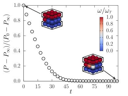
Figure 2: Dissipation power as a function of time for a cubic packing of touching spheres of size $3\times 3\times 3$ with Coulomb friction in the contacts, modeled by Cundall-Strack. The spheres at the bottom plane are constrained to remain static, $\omega_{B}=0$, while those at the top plane rotate with a given angular velocity, $\omega_{T}>0$, as a fixed bearing state. As in the 2d case, here the system evolves to the state of minimum dissipation. In 3d, however, the energy dissipation becomes smaller than when one just splits the system in two domains by the minimum-cut surface, and in the stationary state some spheres do not belong to either of the two fixed bearings. Here $P_{0}$ and $P_{\infty}$ are the initial and stationary dissipation powers, respectively. We also show snapshots of the system, one at the beginning and one at the end of the evolution. The boxes indicate the positions of the imposed boundary conditions.

After a long time, the system reaches a stationary state which, for the Coulomb case, corresponds to a global minimum in dissipated energy since it always decreases monotonically in time. In Fig. 1, we compare viscous damping and Coulomb friction. While in the first case the angular velocities change continuously from top to bottom, for Coulomb friction the system splits in two different fixed bearing states, where the initially free discs in the middle finally follow either the rotating bearing state on the top or the fixed bearing state on the bottom. Between the red and blue regions of Fig. 1 emerges a line of slipping contacts separating the two fixed bearing states.

In the observed stationary states, we find only two domains, one synchronized with each boundary condition. Therefore, in the interface, all slipping contacts have the same relative velocity $\vec{v}_{r(ij)}$. Consequently, the dissipation power $P$ is proportional to the sum of the dynamic friction coefficients in the slipping contacts. We can define a network of contacts where the vertices are the centers of the disks, and an edge exists between any contacting disks. In 2d there is a dual network with vertices in the gaps between spheres. Interestingly, the line of slipping contacts is exactly the minimum cut or shortest weighted path in the dual network, considering as weights of the bonds the friction coefficients of the corresponding contacts, for any distribution of random weights. The shape of the interface should only depend on the friction coefficients and not on the type of bearing states imposed externally. This is indeed the case if one replaces the lower fixed spheres by another non-static bearing state. We can see a close connection of this problem with the max-flow min-cut theorem Elias1956 ; Ford1956 ; Goldberg1988 .

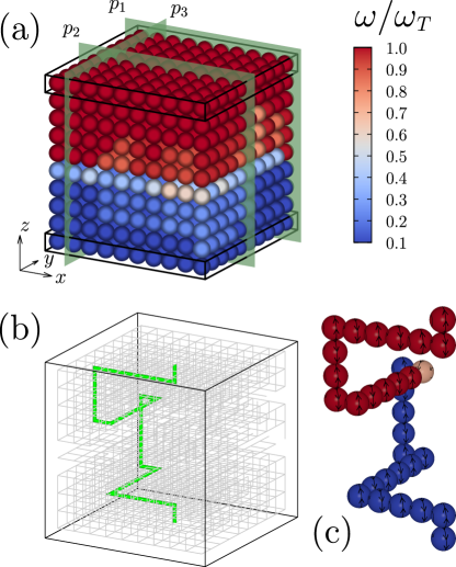
Figure 3: (a) Configuration of minimum dissipation of a cubic packing of size $10\times 10\times 10$ with Coulomb friction in the contacts, obtained with the gradient-descent method. The boxes at the bottom and top indicate the imposed boundary conditions. The spheres at the top and bottom planes are spinning as fixed bearing states with $\omega_{T}=10\omega_{B}$. (b) Network of slipless contacts (in gray) of the configuration shown in (a). The highlighted green path, composed of slipless contacts, connects the top and bottom boundaries. In (c) the spheres along the same path are shown with their corresponding three-dimensional rotations.

In three dimensions, we also observe for viscous damping in the stationary state a continuous transition between the two fixed bearing states. In Fig. 2, we show the dissipation power as a function of time for a $3\times 3\times 3$ system of spheres with Coulomb friction in their contacts. As opposed to two dimensions, we do not find in the stationary state a single surface dividing two different fixed bearing states, but many spheres that do not belong to either of them. In fact, even starting with an initial condition in the minimum-cut configuration, the system evolves towards a stationary state that has a smaller dissipation power. In other words, in the 3d case, the minimum cut in the network of friction coefficients is generally not the state of lowest possible dissipation.

The same behavior is observed for larger systems. In Fig. 3a, we see a $10\times 10\times 10$ cubic bearing, where many spheres in the middle of the bearing are in intermediate bearing states. In this case, the spheres at the top and bottom planes are spinning as fixed bearing states with $\omega_{T}=10\omega_{B}$. For a $32\times 32\times 32$ bearing system, the distribution of power dissipation at the contacts ranges over eleven orders of magnitude (see Supplemental Material SupMat ), although $0.1\leq\mu\leq 1.0$.

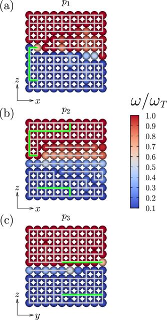
Figure 4: Cuts of the configuration along the three green planes in Fig. 3a. The gray lines correspond to slipless contacts and the green lines correspond to the pieces composing the path, of slipless contacts, that connects bottom and top boundaries, as shown in Fig. 3b.

In this case, due to the large number of possible configurations, we could not determine the exact minimum-cut surface. However, as in the $3\times 3\times 3$ case, Fig. 3a shows that, in the state of minimum dissipated power, some spheres have intermediate angular velocities.

At this point, two relevant questions arise. First, how do these states with dissipation lower than the minimum-cut configuration appear? Second, what are the distinctive properties of these newly discovered stationary states of minimum dissipation? We identified for the configuration shown in Fig. 3a all slipless contacts and discovered that their network spans throughout the system, namely, the two opposite fixed bearing states are connected by paths of slipless contacts as shown in Fig. 3b (gray lines). In Fig. 3b we show one of these paths (highlighted in green), while the spheres along the same path are depicted in Fig. 3c with their corresponding three-dimensional rotations. In two dimensions, as shown in Fig. 1b, we have slip along the entire minimum cut, so that such connecting paths of slipless contacts cannot exist. Therefore a connecting path of slipless contacts, like the green one shown in Fig. 3b, must go through several planes, as shown in Fig. 4. The presence of these paths in the system somehow prevents the global frustration imposed by the fixed bearing states at the bottom and top boundaries. There are a few links through which most connecting paths go, that is, these links have large in-betweeness. In addition, we observe that the network of slipless contacts attains practically every sphere, as depicted in Fig. 3b. Changing the imposed bearing states at the boundaries to other bearing states does not change the network of slipless contacts, showing that, as in two dimensions, it only depends on the disorder in friction coefficients.

The main reason for the difference between two and three dimensions is that in 2d the bearing state has only one degree of freedom, namely, the tangential velocity, while in 3d there are four independent degrees of freedom Baram2004 . In three dimensions, the tangential velocities $\vec{v}_{r(ij)}$ at slipping contacts depend on the sum of two vector products, Eq. (2), which implies a coupling between the components of the angular velocities.

In summary, we found that while for viscous damping there is a continuous change between bearing states, for Coulomb friction jumps appear: In two dimensions, a sharp interface separates the two bearing states, which is identical to the minimum cut. In three dimensions, we discovered a new type of final state in which the network of contacts without slip spans from one fixed bearing state to the other, attaining practically every sphere of the system. Our frustrated bearing in three dimensions with Coulomb friction is an example of a new kind of separation or fracture in a system consisting of an entire set of surfaces and fragments in between, reminiscent of shear failure of rocks under moderate confining pressure. As a future challenge, it would be interesting to study the bottlenecks and their in-betweeness in more detail.

We thank the Brazilian agencies CNPq, CAPES, FUNCAP, and the National Institute of Science and Technology for Complex Systems (INCT-SC) in Brazil for financial support.

References

- (1) H. J. Herrmann, G. Mantica, and D. Bessis, Phys. Rev. Lett. 65, 3223–3226 (1990).
- (2) S. S. Manna and H. J. Herrmann, J. Phys. A: Math. Gen. 24, L481–L490 (1991).
- (3) R. M. Baram, H. J. Herrmann, and N. Rivier, Phys. Rev. Lett. 92, 044301 (2004).
- (4) D. V. Stäger, N. A. M. Araújo, and H. J. Herrmann, Phys. Rev. Lett. 116, 254301 (2016).
- (5) F. Alonso-Marroquin, I. Vardoulakis, H.J. Herrmann, D.Weatherley, P.Mora, Phys. Rev. E 74, 031306 (2006).
- (6) J. E. Ayer and F. E. Soppet, J. Am. Ceram. Soc. 48, 180–183 (1965).
- (7) W. S. Jodrey and E. M. Tory, Phys. Rev. A 32, 2347–2351 (1985).
- (8) A. B. Yu and N. Standish, Powder Technol. 55 171–186 (1988).
- (9) D. Bessis and S. Demko, Commun. Math. Phys. 134, 293–319 (1990).
- (10) Y. Konakawa and K. Ishizaki, Powder Technol. 63, 241–246 (1990).
- (11) N. Standish, A. B. Yu, and R. P. Zou, Powder Technol. 68, 175–186 (1991).
- (12) S. Roux, A. Hansen, H. J. Herrmann, and J.-P. Vilotte, Geophys. Res. Lett. 20, 1499-1502 (1993).
- (13) A. B. Yu and N. Standish, Powder Technol. 76 113–124 (1993).
- (14) S. V. Anishchik and N. N. Medvedev, Phys. Rev. Lett. 75, 4314–4317 (1995).
- (15) J. A. Elliott, A. Kelly, and A. H. Windle, J. Mater. Sci. Lett. 21, 1249–1251 (2002).
- (16) M. P. Ciamarra, A. Coniglio, and M. Nicodemi Phys. Rev. Lett. 97, 158001 (2006).
- (17) J. A. Åström, Eur. Phys. J. E 25, 25–29 (2008).
- (18) T. C. Halsey, Phys. Rev. E 80, 011303 (2009).
- (19) K. Sobolev and A. Amirjanov, Constr. Build. Mater. 24, 1449–1455 (2010).
- (20) S. D. S. Reis, N. A. M. Araújo, J. S. Andrade Jr., and H. J. Herrmann, Europhys. Lett. 97, 18004 (2012).
- (21) M. A. Martín, F. J. Muñoz, M. Reyes, and F. J. Taguas, Pure Appl. Geophys. 172, 141–148 (2015).
- (22) A. Peshkov, M. Girvan, D. C. Richardson, and W. Losert Phys. Rev. E 100, 042905 (2019).
- (23) S. S. Manna and T. Vicsek, J. Stat. Phys. 64, 525–539 (1991).
- (24) G. Oron and H. J. Herrmann, J. Phys. A: Math. Gen. 33, 1417–1434 (2000).
- (25) R. M. Baram and H. J. Herrmann, Fractals 12, 293–301 (2004).
- (26) R. M. Baram and H. J. Herrmann, Phys. Rev. Lett. 95, 224303 (2005).
- (27) J. J. Kranz, N. A. M. Araújo, J. S. Andrade Jr., and H. J. Herrmann, Phys. Rev. E 92, 012802 (2015).
- (28) D. V. Stäger and H. J. Herrmann, Fractals 26, 1850013 (2018).
- (29) N. A. M. Araújo, H. Seybold, R. M. Baram, H. J. Herrmann, and J. S. Andrade Jr., Phys. Rev. Lett. 110, 064106 (2013).
- (30) A. V. Tkachenko and T. A. Witten, Phys. Rev. E 60, 687 (1999).
- (31) J. A. Åström, H. J. Herrmann, and J. Timonen, Phys. Rev. Lett. 84, 638 (2000).
- (32) M. Lätzel, S. Luding, H. J. Herrmann, D. W. Howell, and R. P. Behringer, Eur. Phys. J. E 11, 325 (2003).
- (33) C. Lomnitz, Bull. Seismol. Soc. Am. 72, 1411 (1982).
- (34) Y. Y. Kagan and D. D. Jackson, J. Geophys. Res. 96, 21419 (1991).
- (35) S. Ruder, arXiv:1609.04747 (2016).
- (36) P. A. Cundall and O. D. L. Strack, Geotechnique 29, 47 (1979).
- (37) L. Brendel and S. Dippel, in Physics of Dry Granular Media, edited by H. J. Herrmann, J.-P. Hovi, and S. Luding (Springer, Stuttgart, 1998), p. 313–318.
- (38) C. W. Gear, Math. Comput. 21, 146–156 (1967).
- (39) M. P. Allen and D. J. Tildesley, Computer Simulation of Liquids, (Oxford University Press, Oxford, 1987).
- (40) T. Stegmann, J. Török, L. Brendel, D. E. Wolf, Granular Matter 13, 565–572 (2011).
- (41) I. Prigogine, Science 201, 777–785 (1978).
- (42) P. Elias, A. Feinstein, and C. Shannon, IRE T. Inform. Theory 2, 117–119 (1956).
- (43) L. R. Ford and D. R. Fulkerson, Canadian J. Math. 8, 399–404 (1956).
- (44) A. V. Goldberg and R. E. Tarjan, J. ACM 35, 921–940 (1988).
- (45) See Supplemental Material http://link.aps.org/supplemental/???.