Hydrodynamic transport and violation of the viscosity-to-entropy ratio bound in nodal-line semimetals

Abstract

The ratio between the shear viscosity and the entropy $\eta/s$ is considered a universal measure of the strength of interactions in quantum systems. This quantity was conjectured to have a universal lower bound $(1/4\pi)\hbar/k_{B}$, which indicates a very strongly correlated quantum fluid. By solving the quantum kinetic theory for a nodal-line semimetal in the hydrodynamic regime, we show that $\eta/s\propto T$ violates the universal lower bound, scaling towards zero with decreasing temperature $T$ in the perturbative limit. We find that the hydrodynamic scattering time between collisions is nearly temperature independent, up to logarithmic scaling corrections, and can be extremely short for large nodal lines, near the Mott-Ragel-Ioffe limit. Our finding suggests that nodal-line semimetals can be very strongly correlated quantum systems.

I Introduction

Hydrodynamics describes the behavior of quantum fluids in the regime where the relaxation of electrons is dominated by collision among the quasiparticles. This theory describes long wavelength deviations from local thermal equilibrium, when transport is dominated by conservation laws Hartnoll . Since the time between collisions is the shortest time scale in the problem, the electrons exchange momentum faster than they can relax to phonons or disorder. That leads to universal behavior in the form of a slow diffusion of densities and to viscous flow. This framework has been successfully applied to a variety of different systems, ranging from strong coupling gauge theories with holographic duals Maldacena , quark-gluon plasma Shuryak , cold-atoms systems Joseph ; Clancy , thin wires Moll , and graphene Muller ; Baldurin ; Crossno .

The shear viscosity measures the longitudinal resistivity to transverse gradients in the velocity of a fluid. It has been conjectured by Kovtun et al. Kovtun that quantum systems have a universal lower bound for the ratio between the sheer viscosity and the entropy,

$$\frac{\eta}{s}\geq(1/4\pi)\hbar/k_{B}.$$ (1)

The equality was found in an infinitely strongly coupled field theory and has been associated with “perfect fluids,” systems that are so strongly interacting that they can display quantum turbulence Muller ; Shavit . This ratio is widely believed to be a proxy for the strength of interactions in many classes of quantum systems, including relativistic, non-relativistic systems and Plankian metals Patel , which entirely lack quasiparticles.

By dimensional analysis, the shear viscosity $\eta\sim F\tau$, where $F$ is the free energy and $\tau$ is the relaxation time Zaanen2 ; Zaanen . In hydrodynamic relativistic systems, the free energy is mostly entropic, $F\sim sT$. In the absence of screening, the scattering time due to Coulomb interactions is $\tau\sim\hbar/(k_{B}T)$, and hence $\eta/s\sim\hbar/k_{B}$, with a prefactor of order unity. In general, screened electronic quasiparticles are long lived and typically lead to high viscosity in quantum fluids. In Fermi liquids, the free energy is dominated by the Fermi energy $E_{F}$ at low temperature, whereas $\tau\propto T^{-2}$. The ratio $\eta/s\sim\hbar/k_{B}(E_{F}/T)^{3}$ for $T<E_{F}$ Abrikosov , saturating to a constant $\eta/s\sim\hbar/k_{B}$ at $T>E_{F}$, above the conjectured universal lower bound.

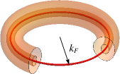
Figure 1: Fermi surface of a NLSM. Massless quasiparticles disperse linearly away from a nodal line (red) with radius $k_{F}$. The toruses enclosing the nodal line are finite energy surfaces. The outer shell with energy $k_{B}\Lambda_{T}$ sets the ultraviolet temperature cut-off of the theory.

Violations of the universal bound were found before in some strongly interacting conformal field theories counter1 ; counter2 ; counter3 and holographic gravity models Hartnoll2 ; Alberte , and were predicted near a superfluid transition Gochan . In quantum materials, it has been recently suggested that anisotropic Dirac fermions found at a topological Lifshitz transition, where two Dirac cones merge Adroguer , violate the proposed lower bound in the non-perturbative regime of interactions Link . Coulomb interactions, nevertheless, were more recently shown to restore the isotropy of the Dirac cone near the fixed point of that problem Kotov2 , effectively reinstating a lower bound. The extent to which the universal lower bound is violated (or not) in that problem requires a closer examination.

In this paper, we show that in nodal systems where the density of states vanishes along a Fermi line, such as in nodal-line semimetals (NLSMs) Burkov ; Mullen ; Yang ; Rappe ; Weng ; Yu ; Heykikila ; Chen ; Xie ; Bian1 ; Bian2 ; Song ; Fu , the ratio between the shear viscosity and the entropy strongly violates the conjectured lower bound, scaling towards zero with decreasing temperature in the perturbative regime,

$$\frac{\eta}{s}\propto\frac{\hbar}{k_{B}}\frac{k_{B}T}{\alpha^{2}v_{F}k_{F}}\sim T\tau,$$ (2)

where $k_{F}$ is the radius of the nodal line, $v_{F}$ is the Fermi velocity of the quasiparticles, and $\alpha=e^{2}/v_{F}$ is the fine structure constant. This is the main result of the paper.

In the absence of screening, the scattering rate $\tau^{-1}$ is set by the volume of the phase space available for collisions. Due to the lack of dispersion along the line, as illustrated in Fig. 1, there is no energy cost for the quasiparticles to scatter in that direction, even at zero temperature. From this phase space argument, the scattering time is hence temperature independent, scales inversely with the length of the nodal line and can be extremely short for large nodal lines, possibly close to the Mott-Ragel-Ioffe limit Ioffe . We find that

$$\tau\sim\frac{\hbar}{\alpha^{2}v_{F}k_{F}},$$ (3)

with additional logarithmic scaling corrections in temperature in the perturbative regime.

We confirm that result by calculating the longitudinal conductivity in the collision dominated regime ($\omega\ll\tau^{-1}$),

$$\sigma(\omega,T)\propto\frac{e^{2}}{h}\frac{k_{B}T}{\alpha^{2}v_{F}}\sim\frac{e^{2}}{h}k_{F}(k_{B}T)\frac{\tau}{\hbar},$$ (4)

which is indicative of insulating behavior. We note that in Weyl semimetals, the dc conductivity $\sigma\propto T^{2}\tau$ also scales linearly with temperature (since $\tau\propto 1/T$, as in graphene note5 ; Parameswaran ), although reflecting a completely distinct behavior in the scaling of the scattering rate, and hence in the viscosity-to-entropy ratio. We conclude that the violation of the bound due to an unusually short and nearly temperature-independent scattering time suggests that NLSMs can be extremely correlated quantum systems.

In the following, we outline the structure of the paper. In Sec. II, we derive the quantum kinetic equation. In Sec. III, we calculate the conductivity in the hydrodynamic regime, including a discussion on many-body effects through a renormalization group analysis. In Sec. IV, we calculate the shear viscosity and demonstrate the violation of the viscosity-to entropy ratio bound. Finally, in Sec. V, we discuss experimental implications of this result.

II Quantum kinetic equation

We adopt the low-energy Hamiltonian of a NLSM that is described by a circular nodal line in the $k_{z}=0$ plane. The low-energy quasiparticles are Dirac fermions located in the vicinity of the nodal line,

$$\mathcal{H}_{0}(\mathbf{k})=\frac{k_{x}^{2}+k_{y}^{2}-k_{F}^{2}}{2m}\sigma_{x}+v_{z}k_{z}\sigma_{y}\approx v_{F}\delta k_{r}\sigma_{x}+v_{z}k_{z}\sigma_{y},$$ (5)

where $\delta k_{r}=k_{r}-k_{F}$ is the in-plane momentum away from the nodal line, and $v_{F}=k_{F}/m$ is the Fermi velocity in the radial direction and $v_{z}$ along the the $z$ direction. The quasiparticles interact through the three-dimensional (3D) Coulomb potential

$$V(q)=4\pi\frac{e^{2}}{q^{2}}$$ (6)

and disperse linearly near the nodal line.

In the hydrodynamic regime, the particles interact with each other more quickly than they lose energy to the lattice. The electronic relaxation is driven by the collision between particles, leading to local thermalization. The out-of-equilibrium distribution function of the quasiparticles $f_{\lambda}(\mathbf{k},\mathbf{x},t)$ satisfies the Boltzmann equation

$$\left(\frac{\partial}{\partial t}+\mathbf{v}_{\lambda,\mathbf{k}}\cdot\nabla_{\mathbf{x}}+e\mathbf{E}\cdot\nabla_{\mathbf{k}}\right)f_{\lambda}=\mathcal{I}_{\textrm{col}}[f_{\lambda}],$$ (7)

where $\lambda=\pm 1$ for quasiparticles and quasiholes respectively, and $\mathbf{v}_{\lambda,\mathbf{k}}=\nabla_{\mathbf{k}}\varepsilon_{\lambda,k}$ is the velocity of the quasiparticles, with

$$\varepsilon_{\lambda,\mathbf{k}}^{0}=\lambda\sqrt{(v_{F}\delta k_{r})^{2}+(v_{z}k_{z})^{2}}$$ (8)

being the equilibrium energy spectrum. The term $e\mathbf{E}=\partial\mathbf{k}/\partial t$ is the external force driving the system, with $\mathbf{E}$ being the electric field, and $\mathcal{I}_{\textrm{col}}[f_{\lambda}]$ is the collision integral, which includes all scattering processes between quasiparticles allowed by Fermi’s golden rule. For a nonequilibrium state,

$$f_{\lambda}\left(\mathbf{k},\mathbf{x},t\right)=f_{\lambda}^{0}\left(\mathbf{k}\right)+\delta f_{\lambda}\left(\mathbf{k},\mathbf{x},t\right),$$ (9)

where $f_{\lambda}^{0}=[e^{\varepsilon_{\lambda}^{0}\beta}+1]^{-1}$ is the equilibrium Fermi distribution, which solves the Boltzmann equation in the absence of interactions $(I_{\text{col}}=0$), $\beta=1/k_{B}T$, and $\delta f_{\lambda}\left(\mathbf{k},\mathbf{x},t\right)$ is the non-equilibrium correction in linear response to an external perturbation such as electric field and strain. In general, $\mathcal{I}_{\textrm{col}}\approx\delta f/\tau$, where $\tau$ is the scattering time between collisions.

III Conductivity

To gain physical intuition in the problem, we derive first the conductivity and the scattering time for NLSMs. If the system is spatially homogenous, the non-equilibrium current carried by the quasiparticles in the presence of an external electric field is

$$\mathbf{J}=e\sum_{\lambda}\int_{\mathbf{k}}\mathbf{v}_{\lambda,\mathbf{k}}f_{\lambda}(\mathbf{k},\omega),$$ (10)

with $\int_{\mathbf{k}}\equiv(2\pi)^{-3}\int\text{d}^{3}k$. In linear response, where $J_{i}=\sigma_{ij}E_{j}$, the conductivity per spin is

$$\sigma_{ij}(\omega,T)=e\sum_{\lambda}\int_{\mathbf{k}}(v_{\lambda,\mathbf{k}})_{i}\frac{\partial}{\partial E_{j}}\delta f_{\lambda}(\mathbf{k},\omega).$$ (11)

In leading order and close to equilibrium, the driving force term on the left-hand side of (7) is

$$-e\mathbf{E}\cdot\nabla_{\mathbf{k}}f_{\lambda}=e\mathbf{E}\cdot\boldsymbol{\phi}_{\lambda}(k)$$ (12)

with $\phi_{\lambda,i}(k)\equiv\beta f_{\lambda}^{0}(1-f_{\lambda}^{0})(v_{\lambda,\mathbf{k}})_{i}.$ The non-equilibrium dispersion can be written in the form

$$\varepsilon_{\lambda,k}=\varepsilon_{\lambda,\mathbf{k}}^{0}+e\mathbf{E}(\omega)\cdot(\nabla_{\mathbf{k}}\varepsilon_{\lambda,k}^{0})g_{\lambda}(k),$$ (13)

with $g_{\lambda}\left(k\right)$ being some unknown function to be found from the solution of the kinetic equation, where $k\equiv(\mathbf{k},\omega)$. With this ansatz, the non-equilibrium correction of the distribution function assumes the form

$$\delta f_{\lambda}\left(k\right)=\beta f_{\lambda}^{0}\left(1-f_{\lambda}^{0}\right)e\mathbf{E}\left(\omega\right)\cdot\mathbf{v}_{\lambda,\mathbf{k}}g_{\lambda}(k).$$ (14)

For convenience, we define $\chi_{\lambda,i}\equiv(v_{\lambda,\mathbf{k}})_{i}g_{\lambda}$. In the collision dominated regime $\omega\ll\tau^{-1}$, the linearized kinetic equation (2) can be approximately expressed in terms of the collision operator as

$$\phi_{\lambda,i}=\mathcal{C}\chi_{\lambda,i},$$ (15)

where

$$\mathcal{C}\chi_{\lambda,i} =\sum_{\lambda_{1}\lambda_{2}\lambda_{3}}\int_{\mathbf{k}_{1}}\int_{\mathbf{k}_{2}}\int_{\mathbf{k}_{3}}\left(2\pi\right)^{4}\delta^{3}\left(\mathbf{k}+\mathbf{k}_{1}-\mathbf{k}_{2}-\mathbf{k}_{3}\right)\delta\left(\varepsilon_{\lambda,\mathbf{k}}^{0}+\varepsilon_{\lambda_{1},\mathbf{k}_{1}}^{0}-\varepsilon_{\lambda_{2},\mathbf{k}_{2}}^{0}-\varepsilon_{\lambda_{3},\mathbf{k}_{3}}^{0}\right)\mathcal{M}_{\lambda\lambda_{1}\lambda_{2}\lambda_{3}}^{\textrm{Col}}f_{\lambda}^{0}f_{\lambda_{1}}^{0}f_{-\lambda_{2}}^{0}f_{-\lambda_{3}}^{0}$$

$$\quad\qquad\qquad\qquad\qquad\qquad\times\left[\chi_{\lambda,i}\left(k\right)+\chi_{\lambda_{1},i}\left(k_{1}\right)-\chi_{\lambda_{2},i}\left(k_{2}\right)-\chi_{\lambda_{3},i}\left(k_{3}\right)\right],$$ (16)

with $\mathcal{M}_{\lambda\lambda_{1}\lambda_{2}\lambda_{3}}^{\textrm{Col}}$ being the collision matrix element Fritz . For details in the derivation of the collision term and integration, see Appendix A.

The solution of the Boltzmann equation requires inverting the collision operator $\mathcal{C}$, which can be done through the standard procedure Fritz . The dominant contribution to the conductivity follows from the eigenfunctions of the collision operator with the lowest eigenvalues. In the collinear approximation, where the momenta of the quasiparticles point in the same direction, the momenta embedded in the definition of the velocities $\mathbf{v}_{\lambda,\mathbf{k}}$ factor out in the integrand of $\mathcal{C}$, which is proportional to

$$\lambda g_{\lambda}\left(k\right)+\lambda_{1}g_{\lambda_{1}}(k_{1})-\lambda_{2}g_{\lambda_{2}}(k_{2})-\lambda_{3}g_{\lambda_{3}}\left(k_{3}\right).$$ (17)

The zero modes of the collision operator $\mathcal{C}\chi_{\lambda,i}=0$ in this restricted phase space are

$$g_{1,\lambda}(k)=a^{(e)}(\omega),$$ (18)

$$g_{2,\lambda}(k)=a^{(\chi)}(\omega)\lambda,$$ (19)

and

$$g_{3,\lambda}(k)=a^{(p)}(\omega)\varepsilon_{\lambda,k}^{0},$$ (20)

corresponding to conservation of charge, chirality, and momentum, respectively.

In the absence of noncollinear processes, those zero modes would produce infinite conductivity Fritz . To account for non-collinear processes, we express the eigenfunctions of full collision operator $\mathcal{C}$ that have the lowest eigenvalues in a basis of zero modes of the collinear regime. We note that due to translational symmetry, the momentum zero mode is an exact eigenfunction of (16), as can be readily checked Fritz ; Kashuba . It does not, however, contribute to the conductivity (11) due to particle-hole symmetry at the nodal line. For the same reason, the chiral modes do not contribute the the charge transport either. We are then left with the charge zero mode, $\chi_{\lambda,i}(k)=a^{(e)}(\omega)(v_{\lambda,\mathbf{k}})_{i}$, which provides the only contribution to the conductivity.

We next restore the frequency dependence of the Boltzmann equation, $\phi_{\lambda,i}=\mathcal{C}\chi_{\lambda,i}+i\omega g_{\lambda}\phi_{\lambda,i}$. In order to calculate the function $a^{(e)}(\omega)$, we define the inner product $(a_{\lambda,i},b_{\lambda,i})=\sum_{\lambda,i}\int_{\mathbf{k}}a_{\lambda,i}(\mathbf{k})b_{\lambda,i}(\mathbf{k})$ and set the variational functional

$$Q\left[a^{(e)}\right]\equiv\left(\chi_{\lambda,i},\phi_{\lambda,i}\right)-\frac{1}{2}\left(\chi_{\lambda,i},\mathcal{C}\chi_{\lambda,i}+i\omega a^{(e)}\phi_{\lambda,i}\right),$$ (21)

which is to be minimized, $\partial Q/\partial a^{(e)}=0.$ The momentum integral of the collision operator is performed in the collinear approximation, where all momenta are nearly parallel to each other. As shown in Appendix B, this approximation is justified by the fact that for a large nodal line ($v_{F}k_{F}\gg k_{B}\Lambda_{T}$), the weight of collinear processes in the collision phase space is logarithmically divergent, as in the case of two-dimensional (2D) Dirac fermions Fritz ; Muller . We also restrict scattering to channels that conserve the number of particles and holes, which are dominant processes in the collinear regime.

Combining the solution of Eq. (21) with Eqs. (11) and (14), we obtain the frequency dependent conductivity in the hydrodynamic regime,

$$\sigma_{ii}(\omega,T)=\gamma_{i}\frac{e^{2}}{h}Nk_{F}\frac{k_{B}T}{i\omega+\alpha^{2}(T)v_{F}(T)k_{F}c(\gamma)},$$ (22)

where

$$\gamma_{z}=\gamma\equiv v_{z}/v_{F},\qquad\gamma_{i}=\gamma^{-1},$$ (23)

for $i=x,y$ and $N$ is the spin degeneracy note6 . The coefficient $c(1)\approx 1.034$ was numerically extracted from the collision integral for $N=2$. This value decreases monotonically away from $\gamma=1$. The functions $\alpha(T)$ and $v_{F}(T)$ are the fine-structure constant and Fermi velocity, respectively, dressed by interaction effects.

III.1 Renormalization group analysis

As in graphene Kotov , Coulomb interactions are marginal and renormalize the velocity of the quasiparticles in the perturbative regime. The velocity grows logarithmically with decreasing temperature,

$$v_{F}(T)=v_{F}\left[1+\frac{\alpha}{4}\ln\left(\frac{\Lambda_{T}}{T}\right)\right],$$ (24)

where $k_{B}\Lambda_{T}=v_{F}\Lambda\ll v_{F}k_{F}$ is the ultraviolet cutoff. The electron charge does not run and the fine-structure constant is also renormalized,

$$\alpha(T)=\frac{\alpha}{1+\frac{\alpha}{4}\ln\left(\Lambda_{T}/T\right)},$$ (25)

and decreases logarithmically at low temperature. The renormalization group (RG) results mimic the structure of the calculation in graphene. The details can be found in Appendix C.

The combination $[\alpha v_{F}]_{(T)}$ does not run, whereas the ratio $\gamma\equiv v_{z}/v_{F}$ flows toward $1$. Hence, in the collision-dominated regime $\omega\ll\tau^{-1}$, $\sigma(0,T)$ scales linearly up to logarithmic corrections, suggesting that the system behaves as an insulator, as shown in Fig. 2(a). In that plot, we use $k_{B}\Lambda_{T}=0.2\times v_{F}k_{F}$, $\gamma=1$ and $\alpha=0.6$. The static charge polarization bubble of a NLSM, $\Pi(q,0)\sim-N/(2\pi)^{3}k_{F}q/v_{F}$, scales linearly with momentum. Since the Coulomb interaction $\propto q^{-2}$, the quasiparticles are partially screened at momenta $q\ll N\alpha k_{F}/2\pi^{2}$, where interactions decay as $\propto q^{-1}$. Below the cut-off temperature $\lambda_{T}/\Lambda_{T}\approx N\alpha k_{F}/2\pi^{2}\Lambda\sim 0.2$, the Coulomb interaction is therefore screened by charge polarization effects, although still long ranged, indicating a crossover in the $T\to 0$ limit. In that regime, the velocity is not further renormalized by the screened Coulomb interaction and the RG flow stops.

A previous on-shell Wilson-Yukawa RG analysis has indicated the presence of a screened interacting fixed point in this problem Huh ; Wang . In the vicinity of that fixed point, a strong charge renormalization was found, suggesting a crossover to a Fermi liquid. We point out that the analysis of Ref. Huh ; Wang did not incorporate the nonanalytic structure of the infrared (IR) polarization bubble in the bosonic propagator, which is relevant in the RG sense. For Dirac fermions, it has been recently shown Kruger that the incorporation of the IR bubble (which is nonanalytic) in the on-shell propagator of the bosons is necessary and correctly recovers previous numerical results based on conformal bootstrap calculations. The fermionic analysis for NLSMs shown above indicates that the charge is not renormalized for $T>\Lambda_{T}$ , whereas the velocity is the only physical quantity that runs in the RG flow in that regime.

From Eq. (22) one can extract the scattering time between collisions,

$$\tau(T)=0.998\times\frac{\hbar}{\alpha^{2}(T)v_{F}(T)k_{F}}.$$ (26)

This is the second main result of the paper. In Fermi liquids, the scattering time diverges as $\tau\propto\hbar\varepsilon_{F}/(k_{B}T)^{2}$, with $\varepsilon_{F}$ the Fermi energy. Relativistic systems have a parametrically shorter scattering time ($\tau\sim\hbar/k_{B}T$), reflecting the absence of screening. The nodal line significantly enlarges the phase space for collisions among the quasiparticles, without producing any screening effects at $T\gtrsim\lambda_{T}$. That further reduces the scattering time, which increases only logarithmically with decreasing temperature, as shown in Fig. 2(b).

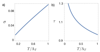
Figure 2: (a) Longitudinal conductivity $\sigma(0,T)$ in units of $e^{2}k_{F}/(h\alpha^{2})$ vs temperature normalized by the ultraviolet temperature cutoff $\Lambda_{T}$ in the collision dominated regime, $\omega\ll\tau^{-1}$. The conductivity has a quasi-linear scaling in the range $T\in[\lambda_{T},T]$, with $\lambda_{T}/\Lambda_{T}\sim 0.2$ (see text). (b) Scattering time $\tau$ in units of $h/\alpha^{2}v_{F}k_{F}$ vs temperature for quasiparticles near the nodal line. In the perturbative regime, $\tau$ scales logarithmically with temperature and has only a modest increase per decade of temperature variation compared to conventional relativistic systems, where $\tau\propto 1/T$.

IV Shear viscosity

The shear viscosity $\eta$ is the dissipative response of fluids to transverse gradients in their velocity field. It is defined after the strain contribution to the stress tensor away from the equilibrium distribution Read

$$\delta\langle T_{ij}\rangle=\eta_{ijk\ell}\frac{\partial u_{k}}{\partial x_{\ell}},$$ (27)

where $\mathbf{u}=\partial\boldsymbol{\xi}/\partial t$ is the velocity field of the fluid, with $\xi_{i}$ being a strain deformation field. The gradient $u_{ij}\equiv\partial u_{i}/\partial x_{j}=\partial\xi_{ij}/\partial t$ is the time derivative of the strain tensor $\xi_{ij}\equiv\partial\xi_{i}/\partial x_{j}$. For systems that preserve time-reversal symmetry, the viscosity tensor is symmetric, obeying the Onsager relation $\eta_{ijk\ell}=\eta_{k\ell ij}$ Avron .

The stress tensor can be derived from the change of the Hamiltonian with respect to the strain tensor,

$$T_{ij}=\frac{\partial\mathcal{H}}{\partial\xi_{ij}}.$$ (28)

In linear response, the first-order contribution of strain to the Hamiltonian can be shown Bradlyn to appear through a term with the general form

$$\mathcal{H}_{\xi}=\frac{1}{2}\xi_{ij}(v_{i}k_{j}+k_{j}v_{i}).$$ (29)

From Eq. (28), the deviation of the expectation value of the stress tensor $\langle T_{ij}\rangle$ away from equilibrium is

$$\delta\langle T_{ij}\rangle=N\sum_{\lambda}\int_{\mathbf{k}}(v_{\lambda,\mathbf{k}})_{i}k_{j}\delta f_{\lambda}(\mathbf{k},t),$$ (30)

from which the shear viscosity in Eq. (27) can be extracted. For details of the derivation, see Appendix D.

Going back to the kinetic equation (7), the second term on the left gives

$$-\mathbf{v}_{\lambda,\mathbf{k}}\cdot\nabla_{\mathbf{x}}f_{\lambda}^{0}\left(k\right)=\beta f_{\lambda}^{0}\left(1-f_{\lambda}^{0}\right)\varepsilon_{\lambda,k}^{0}I_{ij}u_{ij}\equiv\Phi_{\lambda,ij}u_{ij},$$ (31)

with

$$I_{ij}=(v_{\lambda,\mathbf{k}})_{i}k_{j}/\varepsilon_{\lambda,\mathbf{k}}^{0}-(\delta_{ij}/3).$$ (32)

Setting the electric field to zero, the change in the energy spectrum can be parametrized with the ansatz

$$\varepsilon_{\lambda,k}=\varepsilon_{\lambda,k}^{0}+I_{ij}u_{ij}h_{\lambda}\left(\mathbf{k},t\right),$$ (33)

where $h_{\lambda}(\mathbf{k},t)$ is to be determined by solving the kinetic equation. Hence, the nonequilibrium correction to the distribution function due to strain has the form

$$\delta f_{\lambda}\left(\mathbf{k},t\right)=\beta f_{\lambda}^{0}\left(1-f_{\lambda}^{0}\right)u_{ij}I_{ij}h_{\lambda}\left(\mathbf{k},t\right).$$ (34)

Defining $\chi_{\lambda,ij}\equiv I_{ij}h_{\lambda}$, the kinetic equation in the stationary regime ($\omega\to 0$) is

$$\Phi_{\lambda,ij}=\mathcal{C}\chi_{\lambda,ij}.$$ (35)

The definition of the collision operator follows directly from Eq. (16) under the substitution $\chi_{\lambda,i}\to\chi_{\lambda,ij}$. In the collinear regime, there are three zero modes that are eigenfunctions of the collision operator, $\mathcal{C}\chi_{\lambda,ij}=0$, namely,

$$\chi_{\lambda,ij}^{(1)}(\mathbf{k})=\lambda I_{ij},$$ (36)

$$\chi_{\lambda,ij}^{(2)}(\mathbf{k})=\varepsilon_{\lambda,k}^{0}I_{ij}$$ (37)

and

$$\chi_{\lambda,ij}^{(3)}(\mathbf{k})=I_{ij}.$$ (38)

Those modes correspond to conservation of charge, energy, and number of particles respectively. The particle number zero mode, however, does not contribute to the shear viscosity due to particle-hole symmetry at the nodal line. This mode is orthogonal to the other two and can be completely decoupled.

Setting a basis with the charge and energy modes $\chi_{\lambda,ij}^{(\alpha)}(\mathbf{k})$, with $\alpha=1,2$, one can express $\chi_{\lambda,ij}$ as a linear combination in that basis,

$$\chi_{\lambda,ij}(\mathbf{k})=a_{\beta}\chi_{\lambda,ij}^{(\beta)}(\mathbf{k}).$$ (39)

If we project the kinetic equation in that basis, namely

$$b^{\alpha}=(\chi_{\lambda,ij}^{(\alpha)},\Phi_{\lambda,ij}),$$ (40)

and

$$C_{\alpha\beta}=(\chi_{\lambda,ij}^{(\alpha)},\mathcal{C}\chi_{\lambda,ij}^{(\beta)}),$$ (41)

then the solution (39) follows from the determination of the $a_{\beta}$ coefficients

$$a_{\beta}=b^{\alpha}C_{\alpha\beta}^{-1}.$$ (42)

$C_{\alpha\beta}^{-1}$ is the inverse of a $2\times 2$ matrix that can be evaluated numerically through the momentum integration of the collision operator in the collinear approximation, as shown in Appendix C. Substitution in Eqs. (30) and (34) gives the viscosity tensor

$$\eta_{xixi}(T)=c_{i}(\gamma)N\frac{(k_{B}T)^{3}}{\alpha^{2}v_{F}^{3}(T)},\quad i=y,z$$ (43)

where $c_{y}(1)\approx 0.569$ and $c_{z}(1)\approx 0.759$ for $N=2$.

IV.1 Viscosity-entropy ratio

The entropy density of a NLSM can be calculated from the entropy of a noninteracting system dressed by interactions with the renormalized observables,

$$s(T)=-k_{B}N\sum_{\lambda}\int_{\mathbf{k}}f_{\lambda}^{0}\ln f_{\lambda}^{0}=\frac{k_{B}^{3}T^{2}k_{F}}{\gamma v_{F}^{2}(T)}\frac{9}{4}\zeta(3),$$ (44)

where $\zeta(3)\approx 1.20$ is a zeta function. Allowing the Fermi velocity and the fine structure constant to be renormalized according to the RG prescription, the ratio $\eta/s$ is

$$\frac{\eta}{s}=\frac{\hbar}{k_{B}}\gamma c_{i}(\gamma)\frac{4\zeta(3)}{9}\frac{k_{B}T}{\alpha^{2}(T)v_{F}(T)k_{F}}.$$ (45)

In Fig. 3, we plot the temperature dependence of the shear viscosity-entropy ratio in units of $\hbar/k_{B}$ versus temperature in units of the temperature cutoff. The horizontal line is the conjectured lower bound $\eta/s=(1/4\pi)\hbar/k_{B}$. The ratio

$$\frac{\eta}{s}\propto T\left[1+\frac{\alpha}{4}\ln\left(\frac{\Lambda_{T}}{T}\right)\right]$$ (46)

has a quasilinear scaling toward zero with decreasing temperature $T\in[\lambda_{T},\Lambda_{T}]$, in violation of the lower bound. The violation reflects the enlarged phase space for collisions at low temperature in unscreened relativistic systems with a nodal line. For $T\ll\lambda_{T}$, partial screening effects can lead to the restoration of a non-universal lower bound, below the one previously conjectured Kovtun .

Figure 3: Ratio between the sheer viscosity and the entropy, $\eta_{xyxy}/s$ (in units of $\hbar/k_{B}$) vs temperature $T$ normalized by the ultraviolet cutoff $\Lambda_{T}$. We have set the bare fine structure constant $\alpha=0.6$, $\gamma=1$, and $k_{B}\Lambda_{T}=0.2\times v_{F}k_{F}$, with $k_{F}$ being the radius of the nodal line. The horizontal dashed line is the conjectured lower bound, which is violated in NLSMs at sufficiently low temperature. At $T\ll\lambda_{T}\sim 0.2\Lambda_{T}$, Coulomb interactions are partially screened by charge polarization effects, suggesting a crossover (see text).

V Discussion

In the hydrodynamic regime, the usual manifestations of the viscous flow of electrons in constrained geometries include nonlocal negative resistance Baldurin ; Crossno ; Levitov and fluid dynamics with vortex lines Barenghia . The very low viscosity compared to the amount of entropy production, in violation of the conjectured lower bound, is highly suggestive that NLSMs may exhibit quantum turbulence Muller ; Shavit ; Barenghia .

In general, observation of hydrodynamics requires quasiparticles with a relatively short scattering time. Signatures of hydrodynamic behavior can be detected in the collision-dominated regime through optical and transport measurements when $k_{B}T\gg\varepsilon_{F},\,\Delta$, with $\varepsilon_{F}$ being the energy of the Fermi surface and $\Delta$ being the gap induced by spin-orbit coupling effects or possible many-body instabilities Nandkishore ; Roy , including excitonic phases Rudenko . NLSMs that combine inversion, time reversal, and mirror glide symmetry have nodal lines that are robust against spin-orbit coupling Nelson .

NLSMs are unique in that the nodal line introduces a length scale that does not generate fully screned interactions, as in Fermi liquids. That length scale substantially enlarges the size of the phase space for collision of thermally excited quasiparticles and is responsible for the unusual temperature scaling of the scattering time in the hydrodynamic regime. Materials such as ZrSiSe Shao have a large nodal line gapped by a small spin-orbit coupling gap of $\Delta\approx 30$ meV, with $v_{F}\Lambda\approx 0.4$ eV $(\Lambda_{T}\approx 4\times 10^{3}K)$ and $v_{F}k_{F}\approx 2$eV. In this material, the Fermi velocity $\hbar v_{F}\approx 2$eVÅ is three times smaller than in graphene. Experimental control over the value of the fine structure constant can be achieved with experiments on thin films encapsulated by dielectric materials. In ZrSiSe, for a moderate fine structure constant $\alpha\approx 0.6$ within the perturbative regime, the scattering length at $T\gg\Delta/k_{B}$,

$$\ell_{s}=v_{F}\tau\sim\frac{\hbar v_{F}}{\alpha^{2}v_{F}k_{F}},$$ (47)

is of the order of the lattice constant, near the Mott-Ragel-Ioffe limit, indicating the presence of very strong correlations. We speculate that hydrodynamic behavior may be observable in a number of different NLSM materials.

VI Acknowledgements

B. U. thanks V. N. Kotov for helpful discussions. The authors acknowledge the Carl T. Bush Fellowship for partial support. B. U. acknowledges NSF Grant DMR-2024864 for support.

Appendix A Quantum kinetics in the hydrodynamic regime

Following the derivation of Kadanoff (Kadanoff, ), the Boltzmann equation has the general form:

$$\left(\frac{\partial}{\partial t}+\mathbf{v}_{\lambda,\mathbf{k}}\cdot\nabla_{\mathbf{x}}+e\mathbf{E}\cdot\nabla_{\mathbf{k}}\right)f_{\lambda}(\mathbf{x},\mathbf{k},t)=\mathcal{I}_{\textrm{col}}[f_{\lambda}],$$ (48)

where $-\nabla_{\mathbf{x}}U_{\textrm{ext}}\left(\boldsymbol{x},t\right)=e\mathbf{E}$ is the external force, $f_{\lambda}\left(\mathbf{x},k,t\right)$ is the nonequilibrium Fermi distribution, and

$$\mathcal{I}_{\textrm{col}}[f_{\lambda}] =-f_{\lambda}\left(k,t\right)\left(\bar{\Sigma}_{\lambda,\lambda}^{>}\left(k,t\right)\right)_{\omega=\varepsilon_{\lambda}}$$

$$+\left(1-f_{\lambda}\left(k,t\right)\right)\left(\bar{\Sigma}_{\lambda,\lambda}^{<}\left(k,t\right)\right)_{\omega=\varepsilon_{\lambda}}$$ (49)

is the collision term, with

$$\left(\bar{\Sigma}_{\lambda,\lambda}^{>}\right)_{\omega=\varepsilon_{\lambda}} =\sum_{\lambda_{1}\lambda_{2}\lambda_{3}}\int_{\mathbf{k}_{1}}\int_{\mathbf{k}_{2}}\int_{\mathbf{k}_{3}}\left(2\pi\right)^{4}\delta\left(\mathbf{p}+\mathbf{p}_{1}-\mathbf{p}_{2}-\mathbf{p}_{3}\right)\delta\left(\varepsilon_{\lambda,k}+\varepsilon_{\lambda_{1},k_{1}}-\varepsilon_{\lambda_{2},k_{2}}-\varepsilon_{\lambda_{3},k_{3}}\right)$$

$$\times\left[NV\left(\mathbf{k}-\mathbf{k}_{2}\right)V\left(\mathbf{k}-\mathbf{k}_{2}\right)M_{\lambda_{3}\lambda_{1}}M_{\lambda_{1}\lambda_{3}}M_{\lambda\lambda_{2}}M_{\lambda_{2}\lambda}f_{\lambda_{1}}\left(1-f_{\lambda_{2}}\right)\left(1-f_{\lambda_{3}}\right)\right.$$

$$\left.-V\left(\mathbf{k}-\mathbf{k_{2}}\right)V\left(\mathbf{k}-\mathbf{k_{3}}\right)M_{\lambda\lambda_{2}}M_{\lambda_{2}\lambda_{1}}M_{\lambda_{1}\lambda_{3}}M_{\lambda_{3}\lambda}f_{\lambda_{1}}\left(1-f_{\lambda_{2}}\right)\left(1-f_{\lambda_{3}}\right)\right]$$ (50)

$$\left(\bar{\Sigma}_{\lambda,\lambda}^{<}\right)_{\omega=\varepsilon_{\lambda}} =\left\{f\leftrightarrow 1-f\right\}.$$ (51)

$V\left(\mathbf{k}\right)=4\pi e^{2}/\mathbf{k}^{2}$ is the Coulomb interaction and $M$ is a tensor in the quasiparticle-hole basis. Explicitly,

$$M_{\lambda\lambda_{1}}\left(\mathbf{\mathbf{k}},\mathbf{k}_{1}\right)\equiv\left[U_{\mathbf{\mathbf{k}}}^{-1}U_{\mathbf{k}_{1}}\right]_{\lambda\lambda_{1}},$$ (52)

with $U_{\mathbf{k}}$ being a unitary transformation that diagonalizes the Hamiltonian.

For nodal-line semimetals (NLSMs),

$$\mathcal{H}_{0} =\frac{k_{r}^{2}-k_{F}^{2}}{2m}\sigma_{x}+v_{z}k_{z}\sigma_{y}$$

$$\approx\frac{\left(2k_{F}\right)\left(k_{r}-k_{F}\right)}{2m}\sigma_{x}+v_{z}k_{z}\sigma_{y}$$

$$=v_{F}\delta k_{r}\sigma_{x}+v_{z}\delta k_{z}\sigma_{y}$$

$$\equiv v_{F}\left(h_{x}\sigma_{x}+h_{y}\sigma_{y}\right),$$ (53)

or

$$\mathcal{H}_{0}=\left(\begin{array}[]{cc}0&\mathsf{H}\\ \mathsf{H}^{*}&0\end{array}\right),$$ (54)

where $\mathsf{H}=h_{x}+ih_{y}$,

$$\left|\mathbf{h}\right|=\left|\mathsf{H}\right|=\sqrt{\left(h_{x}\right)^{2}+\left(h_{y}\right)^{2}}=h.$$

$\delta\mathbf{k}$ is a relative momentum from the node line. The Hamiltonian can be diagonalized in the quasi-particle and quasi-hole basis with their energy $\pm v_{F}h$. We assign each basis as $\lambda=\pm 1$, and thus $\varepsilon_{\lambda,k}=\lambda v_{F}h$ where $\lambda=+1$ corresponds to a excited particle and $\lambda=-1$ to a excited hole. The unitary transformation matrix is

$$U_{\mathbf{k}}=\frac{1}{\sqrt{2}}\left(\begin{array}[]{cc}1&1\\ \mathsf{H}/h&-\mathsf{H}/h\end{array}\right),$$ (55)

and thus, the tensor $M$ is

$$M_{\lambda\lambda_{1}}\left(\mathbf{\mathbf{k}},\mathbf{k}_{1}\right)=\frac{1}{2}\left(1+\lambda\lambda_{1}\frac{\mathsf{H}^{*}\mathsf{H}_{1}}{hh_{1}}\right).$$ (56)

The velocity of quasiparticles in the Boltzmann equation is, by definition,

$$\mathbf{v}_{\lambda,\mathbf{k}} =\frac{\partial\varepsilon_{\lambda,k}}{\partial k_{i}}$$

$$=\frac{\lambda v_{F}}{h}\left(h_{x}\frac{\partial h_{x}}{\partial k_{x}},h_{x}\frac{\partial h_{x}}{\partial k_{y}},h_{y}\frac{\partial h_{y}}{\partial k_{z}}\right).$$ (57)

A.1 Linearized Boltzmann equation

Starting from the the nonequilibrium correction of the distribution function due to the presence of an external electric field,

$$\delta f_{\lambda}\left(\mathbf{k},\omega\right)=\beta f_{\lambda}^{0}\left(1-f_{\lambda}^{0}\right)e\mathbf{E}\left(\omega\right)\cdot\mathbf{v}_{\lambda,\mathbf{k}}g_{\lambda}(\mathbf{k},\omega).$$ (58)

where $\chi_{\lambda,i}\equiv(v_{\lambda,\mathbf{k}})_{i}g_{\lambda}$, with $g_{\lambda}$ being a function to be determined by solving the quantum kinetic equation (7). The left-hand side of that equation is

$$\left(i\omega\chi_{\lambda}\left(k,\omega\right)-1\right)\beta eE_{i}\left(\omega\right)\left(\mathbf{v}_{\mathbf{k}}\right)_{i}f_{\lambda}^{0}\left(1-f_{\lambda}^{0}\right).$$ (59)

Defining $f_{\lambda_{i}}\equiv f_{\lambda_{i}}\left(k_{i}\right)$, the collision term in the right-hand side is

$$\mathcal{I}_{\text{col}}[f_{\lambda}] =\sum_{\lambda_{1}\lambda_{2}\lambda_{3}}\int_{\mathbf{k}_{1}}\int_{\mathbf{k}_{2}}\int_{\mathbf{k}_{3}}\left(2\pi\right)^{4}\delta^{3}\left(\mathbf{k}+\mathbf{k}_{1}-\mathbf{k}_{2}-\mathbf{k}_{3}\right)\delta\left(\varepsilon_{\lambda}+\varepsilon_{\lambda_{1}}-\varepsilon_{\lambda_{2}}-\varepsilon_{\lambda_{3}}\right)$$

$$\times\left[NV\left(\mathbf{k}-\mathbf{k}_{2}\right)^{2}W_{\lambda\lambda_{1}\lambda_{2}\lambda_{3}}-V\left(\mathbf{k}-\mathbf{k_{2}}\right)V\left(\mathbf{k}-\mathbf{k_{3}}\right)Y_{\lambda\lambda_{1}\lambda_{2}\lambda_{3}}\right]$$

$$\times\left[\left(1-f_{\lambda}\right)\left(1-f_{\lambda_{1}}\right)f_{\lambda_{2}}f_{\lambda_{3}}-f_{\lambda}f_{\lambda_{1}}\left(1-f_{\lambda_{2}}\right)\left(1-f_{\lambda_{3}}\right)\right],$$ (60)

with $N$ being the fermionic degeneracy, and

$$W_{\lambda\lambda_{1}\lambda_{2}\lambda_{3}} =M_{\lambda\lambda_{2}}M_{\lambda_{2}\lambda}M_{\lambda_{3}\lambda_{1}}M_{\lambda_{1}\lambda_{3}}$$

$$Y_{\lambda\lambda_{1}\lambda_{2}\lambda_{3}} =M_{\lambda\lambda_{2}}M_{\lambda_{1}\lambda_{3}}M_{\lambda_{3}\lambda}M_{\lambda_{2}\lambda_{1}},$$ (61)

where $M_{\lambda\lambda_{1}}\equiv M_{\lambda\lambda_{1}}(\mathbf{k},\mathbf{k}_{1})$, and so on.

The third line of (60) has two terms with four $f$ functions. One should expand it in eight terms to linear order in $\delta f$, with three $f^{0}$ and one $\delta f$. We can simplify them using

$$f_{-\lambda}^{0}f_{-\lambda_{1}}^{0}f_{\lambda_{2}}^{0}f_{\lambda_{3}}^{0} =e^{\left(\lambda v_{r}k^{\prime}+\lambda v_{r}k_{1}^{\prime}\right)\beta}f_{\lambda}^{0}f_{\lambda_{1}}^{0}f_{\lambda_{2}}^{0}f_{\lambda_{3}}^{0}$$

$$=e^{\left(\lambda v_{r}k_{2}^{\prime}+\lambda v_{r}k_{3}^{\prime}\right)\beta}f_{\lambda}^{0}f_{\lambda_{1}}^{0}f_{\lambda_{2}}^{0}f_{\lambda_{3}}^{0}$$

$$=f_{\lambda}^{0}f_{\lambda_{1}}^{0}f_{-\lambda_{2}}^{0}f_{-\lambda_{3}}^{0}.$$ (62)

which is restricted by the energy conservation. After some straightforward algebra, we find

$$\mathcal{I}_{\text{col}}[f_{\lambda}]= -\sum_{\lambda_{1}\lambda_{2}\lambda_{3}}\int_{\mathbf{k}_{1}}\int_{\mathbf{k}_{2}}\int_{\mathbf{k}_{3}}\left(2\pi\right)^{4}\delta^{3}\left(\mathbf{k}+\mathbf{k}_{1}-\mathbf{k}_{2}-\mathbf{k}_{3}\right)\delta\left(\varepsilon_{\lambda}+\varepsilon_{\lambda_{1}}-\varepsilon_{\lambda_{2}}-\varepsilon_{\lambda_{3}}\right)$$

$$\times\left[NV^{2}\left(\mathbf{k}-\mathbf{k}_{2}\right)W_{\lambda\lambda_{1}\lambda_{2}\lambda_{3}}-V\left(\mathbf{k}-\mathbf{k}_{2}\right)V\left(\mathbf{k}-\mathbf{k}_{3}\right)Y_{\lambda\lambda_{1}\lambda_{2}\lambda_{3}}\right]\beta eE_{i}\left(\omega\right)f_{\lambda}^{0}f_{\lambda_{1}}^{0}f_{-\lambda_{2}}^{0}f_{-\lambda_{3}}^{0}$$

$$\times\left[\chi_{i}\left(\lambda,k\right)+\chi_{i}\left(\lambda_{1},k_{1}\right)-\chi_{i}\left(\lambda_{2},k_{2}\right)-\chi_{i}\left(\lambda_{3},k_{3}\right)\right],$$ (63)

with the collision matrix element

$$\mathcal{M}_{\lambda\lambda_{1}\lambda_{2}\lambda_{3}}^{\text{Col}}=NV^{2}\left(\mathbf{k}-\mathbf{k}_{2}\right)W_{\lambda\lambda_{1}\lambda_{2}\lambda_{3}}-V\left(\mathbf{k}-\mathbf{k}_{2}\right)V\left(\mathbf{k}-\mathbf{k}_{3}\right)Y_{\lambda\lambda_{1}\lambda_{2}\lambda_{3}}.$$ (64)

Defining

$$\phi_{\lambda,i}(k)\equiv\beta f_{\lambda}^{0}(1-f_{\lambda}^{0})(v_{\lambda,\mathbf{k}})_{i},$$ (65)

equating the left- and the right-hand side of the quantum Boltzmann equation, Eq. (59) and (63), we have

$$\phi_{\lambda,i}=\mathcal{C}\chi_{\lambda,i}+i\omega g_{\lambda}\phi_{\lambda,i},$$ (66)

with $\mathcal{C}$ being the collision operator as defined in the main text,

$$\mathcal{C}\chi_{\lambda,i} =\sum_{\lambda_{1}\lambda_{2}\lambda_{3}}\int_{\mathbf{k}_{1}}\int_{\mathbf{k}_{2}}\int_{\mathbf{k}_{3}}\left(2\pi\right)^{4}\delta^{3}\left(\mathbf{k}+\mathbf{k}_{1}-\mathbf{k}_{2}-\mathbf{k}_{3}\right)\delta\left(\varepsilon_{\lambda,k}^{0}+\varepsilon_{\lambda_{1},k_{1}}^{0}-\varepsilon_{\lambda_{2},k_{2}}^{0}-\varepsilon_{\lambda_{3},k_{3}}^{0}\right)\mathcal{M}_{\lambda\lambda_{1}\lambda_{2}\lambda_{3}}^{\textrm{Col}}$$

$$\quad\qquad\qquad\times f_{\lambda}^{0}f_{\lambda_{1}}^{0}f_{-\lambda_{2}}^{0}f_{-\lambda_{3}}^{0}\left[\chi_{\lambda,i}\left(k\right)+\chi_{\lambda_{1},i}\left(k_{1}\right)-\chi_{\lambda_{2},i}\left(k_{2}\right)-\chi_{\lambda_{3},i}\left(k_{3}\right)\right].$$ (67)

Appendix B Collinear approximation

B.1 Collision phase space

Due to the Coulomb potential $V\left(\mathbf{k}-\mathbf{k}_{2}\right)$ and $V\left(\mathbf{k}-\mathbf{k}_{3}\right)$ in the integrand of the collision operator, the integral is governed by small momentum transfer due to collision processes. In the collinear approximation, where the four momenta are nearly aligned to each other around the nodal line, we can define the momenta

$$\mathbf{k} =\left(k_{r},0,k_{z}\right)=\left(\delta k_{r}+k_{F},0,k_{z}\right)$$ (68)

$$\mathbf{k}_{1} \approx\left(k_{1r},k_{1\perp},k_{1z}\right)=\left(\delta k_{1r}+k_{F},k_{1\perp},k_{1z}\right)$$ (69)

$$\mathbf{k}_{2} \approx\left(k_{2r},k_{2\perp},k_{2z}\right)=\left(\delta k_{2r}+k_{F},k_{2\perp},k_{2z}\right)$$ (70)

$$\mathbf{k}_{3} \approx\left(k_{3r},k_{3\perp},k_{3z}\right)=\left(\delta k_{3r}+k_{F},k_{3\perp},k_{3z}\right),$$ (71)

where we assume that the $\perp$ components are small compared to the radius of the nodal line $k_{F}$. The phase space for collision processes is set by conservation of energy,

$$\delta\left(\varepsilon_{\lambda,\mathbf{k}}^{0}+\varepsilon_{\lambda_{1},\mathbf{k}_{1}}^{0}-\varepsilon_{\lambda_{2},\mathbf{k}_{2}}^{0}-\varepsilon_{\lambda_{3},\mathbf{k}_{3}}^{0}\right).$$

We now expressing it in terms of the dimensionless variables,

$$x\equiv v_{F}\beta(\delta k_{r}) ,\qquad y\equiv v_{z}\beta k_{z},\qquad\kappa_{0}\equiv v_{F}k_{F}\beta,\qquad r^{2}\equiv x^{2}+y^{2},$$ (72)

and

$$x_{n}\equiv v_{F}\beta(\delta k_{nr}) ,\qquad y_{n}\equiv v_{z}\beta k_{nz},\qquad\xi_{n}\equiv v_{F}\beta k_{n\perp},\qquad r_{n}^{2}\equiv x_{n}^{2}+y_{n}^{2},$$ (73)

with $n=1,2,3$. Performing a suitable change of variables $\mathbf{k}_{2}\to\mathbf{k}-\mathbf{k}_{2}$ and $\mathbf{k}_{3}\to\mathbf{k}_{1}-\mathbf{k}_{3}$,

$$\beta\delta(D)\equiv\delta\left(\varepsilon_{\lambda,\mathbf{k}}^{0}+\varepsilon_{\lambda_{1},\mathbf{k}_{1}}^{0}-\varepsilon_{\lambda_{2},\mathbf{k}+\mathbf{k}_{2}}^{0}-\varepsilon_{\lambda_{3},\mathbf{k}_{1}-\mathbf{k}_{3}}^{0}\right),$$ (74)

where

$$D =\lambda r+\lambda_{1}\sqrt{\left(x_{1}+\frac{\xi_{1}^{2}}{2\kappa_{0}}\right)^{2}+y_{1}^{2}}-\lambda_{2}\sqrt{\left(x+x_{2}+\frac{\xi_{2}^{2}}{2\kappa_{0}}\right)^{2}+\left(y+y_{2}\right)^{2}}-\lambda_{3}\sqrt{\left(x_{1}-x_{2}+\frac{\left(\xi_{1}-\xi_{2}\right)^{2}}{2\kappa_{0}}\right)^{2}+\left(y_{1}-y_{2}\right)},$$ (75)

while at the same time

$$V\left(\mathbf{k}-\mathbf{k}_{2}\right)\longrightarrow\bar{V_{1}} =\frac{1}{\left(x_{2}\right)^{2}+\gamma^{-2}\left(y_{2}\right)^{2}+\left(\xi_{2}\right)^{2}}$$ (76)

$$V\left(\mathbf{k}-\mathbf{k}_{3}\right)\longrightarrow\bar{V_{2}} =\left(\frac{1}{\left(x-x_{1}+x_{2}\right)^{2}+\gamma^{-2}\left(y-y+y_{2}\right)^{2}+\left(\xi_{1}-\xi_{2}\right)^{2}}\right),$$ (77)

after using momentum conservation $\mathbf{k}+\mathbf{k}_{1}-\mathbf{k}_{2}-\mathbf{k}_{3}=0$.

Since $\xi_{1}$ and $\xi_{2}$ are much smaller than $\kappa_{0}$, we can rewrite the argument of the $\delta$ function $D$ as

$$D \approx\bar{A}+\lambda_{1}\frac{x_{1}\xi_{1}^{2}}{2r_{1}\kappa_{0}}-\lambda_{2}\frac{\left(x+x_{2}\right)\xi_{2}^{2}}{2\left|\mathbf{r}+\mathbf{r}_{2}\right|\kappa_{0}}-\lambda_{3}\frac{\left(x_{1}-x_{2}\right)\left(\xi_{1}-\xi_{2}\right)^{2}}{2\left|\mathbf{r}_{1}-\mathbf{r}_{2}\right|\kappa_{0}}$$

$$=-\left(\frac{\lambda_{3}\left(x_{1}-x_{2}\right)}{2\left|\mathbf{r}_{1}-\mathbf{r}_{2}\right|\kappa_{0}}+\frac{\lambda_{2}\left(x+x_{2}\right)}{2\left|\mathbf{r}+\mathbf{r}_{2}\right|\kappa_{0}}\right)\xi_{2}^{2}+\frac{\lambda_{3}\left(x_{1}-x_{2}\right)}{\left|\mathbf{r}_{1}-\mathbf{r}_{2}\right|\kappa_{0}}\xi_{1}\xi_{2}-\left(\frac{\lambda_{3}\left(x_{1}-x_{2}\right)}{2\left|\mathbf{r}_{1}-\mathbf{r}_{2}\right|\kappa_{0}}-\frac{\lambda_{1}x_{1}}{2r_{1}\kappa_{0}}\right)\xi_{1}^{2}+\bar{A}$$

$$\equiv-\frac{w_{1}}{2\kappa_{0}}\left(\xi_{1}^{2}-2\frac{w_{2}}{w_{1}}\xi_{2}\xi_{1}+\frac{w_{3}}{w_{1}}\xi_{2}^{2}-\frac{\bar{A}}{w_{1}}\right)$$ (78)

where

$$\bar{A} \equiv\lambda r+\lambda_{1}r_{1}-\lambda_{2}\left|\mathbf{r}+\mathbf{r}_{2}\right|-\lambda_{3}\left|\mathbf{r}_{1}-\mathbf{r}_{2}\right|$$ (79)

$$\left|\mathbf{r}+\mathbf{r}_{2}\right| \equiv\sqrt{\left(x+x_{2}\right)^{2}+\left(y+y_{2}\right)^{2}}$$ (80)

$$\left|\mathbf{r}_{1}-\mathbf{r}_{2}\right| \equiv\sqrt{\left(x_{1}-x_{2}\right)^{2}+\left(y_{1}-y_{2}\right)^{2}},$$ (81)

and $w_{i}$ ($i=1,2,3$) are functions of the dimensionles variables $x,y,x_{i},y_{i}$. $D$ is a quadratic function of $\xi_{1}$. We can then express the $\delta$ function as

$$\delta\left(\bar{D}\left(\xi_{1}\right)\right)=\sum_{i=\pm}\frac{\delta\left(\xi_{1}-\xi_{i}\right)}{\left|D^{\prime}\left(\xi_{i}\right)\right|},$$ (82)

where $D^{\prime}$ is the first derivative of $D$, and $\xi_{i=\pm}$ are the two roots of the quadratic function, namely

$$\xi_{\pm}=\frac{w_{2}}{w_{1}}\xi_{2}\pm\sqrt{\left(\frac{w_{2}}{w_{1}}\xi_{2}\right)^{2}-\left(\frac{w_{3}}{w_{1}}\xi_{2}^{2}-\frac{\bar{A}}{w_{1}}\right)}.$$ (83)

Hence,

$$\left|\bar{D}^{\prime}\left(\xi_{i}\right)\right| =\left|\frac{w_{1}}{2\kappa_{0}}\left[\left(2\xi_{1}-\xi_{+}-\xi_{-}\right)\right]_{\xi_{1}=\xi_{i}}\right|$$

$$=\left|\frac{w_{1}}{2\kappa_{0}}\left(\xi_{+}-\xi_{-}\right)\right|$$

$$=\left|\frac{w_{1}}{2\kappa_{0}}\sqrt{\left(\frac{w_{2}}{w_{1}}\xi_{2}\right)^{2}-\left(\frac{w_{3}}{w_{1}}\xi_{2}^{2}-\frac{\bar{A}}{w_{1}}\right)}\right|.$$ (84)

Thus,

$$\delta\left(D\left(\xi_{1}\right)\right) =\kappa_{0}\left|\frac{1}{\sqrt{\left(w_{1}w_{2}\xi_{2}\right)^{2}-\left(w_{1}w_{3}\xi_{2}^{2}-w_{1}\bar{A}\right)}}\right|$$ (85)

$$\quad\times\left(\delta\left(\xi_{1}-\xi_{1+}\right)+\delta\left(\xi_{1}-\xi_{1-}\right)\right)$$ (86)

It is clear that the phase space has a logarithmic divergence in the $\xi_{2}$ variable when $\bar{A}\rightarrow 0$. At the same time, the Coulomb interaction terms $\bar{V}_{1}$ and $\bar{V}_{2}$ defined in Eqs. (76) and (77) decay quickly to zero with $\xi_{2}$ when it is large. Thus, there are two important regions of the integrand in phase space: $\bar{A}\rightarrow 0$ and $\xi_{2}\rightarrow 0$. This phase space argument justifies the validity of the collinear approximation, with which the conductivity and the shear viscosity were calculated.

B.1.1 Calculation of the conductivity

The variational functional of the conductivity is

$$Q\left[a^{(e)}\right]\equiv\left(\chi_{\lambda,i},\phi_{\lambda,i}\right)-\frac{1}{2}\left(\chi_{\lambda,i},C\chi_{\lambda,i}+i\omega a^{(e)}\phi_{\lambda,i}\right).$$ (87)

We define the inner product $(a_{\lambda,i},b_{\lambda,i})\equiv\sum_{\lambda,i}\int_{\mathbf{k}}a_{\lambda,i}(\mathbf{k})b_{\lambda,i}(\mathbf{k})$, with

$$\frac{\partial Q}{\partial a^{(e)}}=0,$$

with $a^{(e)}(\omega)$ being the variational function corresponding to charge conservation in the collinear regime. For convenience, after multiplying the factor $v_{F}\beta^{3}$ in both sides of Eq. (87), the first term is

$$v_{z}\beta^{3}\left(\chi_{\lambda,i},\phi_{\lambda,i}\right) =a^{(e)}v_{F}\beta^{3}\sum_{\lambda}\int_{\mathbf{k}}\lambda^{2}v_{r}^{2}\int\frac{d^{3}k}{\left(2\pi\right)^{3}}\frac{1}{\left(e^{\lambda v_{r}h\beta}+1\right)\left(e^{-\lambda v_{r}h\beta}+1\right)}$$

$$=a^{(e)}\frac{v_{F}k_{F}\beta}{\pi}\left(\gamma^{-1}+\gamma\right)\int dr\frac{r}{\left(e^{r}+1\right)\left(e^{-r}+1\right)}$$

$$=a^{(e)}\kappa_{0}\frac{\ln\left(2\right)}{2\pi}\left(\gamma^{-1}+\gamma\right),$$ (88)

where $\gamma\equiv v_{z}/v_{F}$, and

$$\int\frac{d^{3}k}{\left(2\pi\right)^{3}}\rightarrow\int k_{F}\frac{dk_{r}\,dk_{z}}{\left(2\pi\right)^{3}}d\phi\rightarrow k_{F}\int\frac{d\delta k_{r}\,d\delta k_{z}}{\left(2\pi\right)^{3}}d\phi\rightarrow\frac{k_{F}}{v_{r}v_{z}\beta^{2}}\int\frac{dx\,dy}{\left(2\pi\right)^{3}}d\phi.$$ (89)

To calculate the second term, we consider the dominant processes in the near collinear regime, which conserve the number of particles and holes. We have

$$\frac{v_{F}\beta^{3}}{2}\left(\chi_{\lambda,i},\mathcal{C}\chi_{\lambda,i}+i\omega a^{(e)}\phi_{\lambda,i}\right) =\frac{v_{F}\beta^{3}}{8}\sum_{\lambda_{i}}\int\frac{d^{3}k}{\left(2\pi\right)^{3}}\frac{d\delta k_{1r}d\delta k_{1z}dk_{1\perp}}{\left(2\pi\right)^{3}}\frac{d\delta k_{2r}d\delta k_{2r}dk_{2\perp}}{\left(2\pi\right)^{3}}\frac{d\delta k_{3r}d\delta_{3r}dk_{3\perp}}{\left(2\pi\right)^{3}}$$

$$\qquad\times 2\pi\delta\left(\lambda v_{F}h+\lambda_{1}v_{F}h_{1}-\lambda_{2}v_{F}h_{2}-\lambda_{3}v_{F}h_{3}\right)\left(2\pi\right)^{3}\delta^{3}\left(\mathbf{k}+\mathbf{k}_{1}-\mathbf{k}_{2}-\mathbf{k}_{3}\right)$$

$$\qquad\times f_{\lambda}^{0}f_{\lambda_{1}}^{0}f_{-\lambda_{2}}^{0}f_{-\lambda_{3}}^{0}\left[NV^{2}\left(\mathbf{k}-\mathbf{k}_{2}\right)W_{\lambda\lambda_{1}\lambda_{2}\lambda_{3}}-V\left(\mathbf{k}-\mathbf{k}_{2}\right)V\left(\mathbf{k}-\mathbf{k}_{3}\right)Y_{\lambda\lambda_{1}\lambda_{2}\lambda_{3}}\right]$$

$$\qquad\times\left(a^{(e)}\right)^{2}\left[\mathbf{v}_{\lambda,\mathbf{k}}+\mathbf{v}_{\lambda_{1},\mathbf{k}_{1}}-\mathbf{v}_{\lambda_{2},\mathbf{k}_{2}}-\mathbf{v}_{\lambda_{3},\mathbf{k}_{3}}\right]^{2}+\frac{i\omega}{2}\left(a^{(e)}\right)^{2}\kappa_{0}\frac{\ln\left(2\right)}{\pi}\left(\gamma^{-1}+\gamma\right)$$

$$\equiv\frac{\kappa_{0}^{2}\alpha^{2}}{\beta}\left[a^{(e)}\right]^{2}I(\gamma)+i\omega\left[a^{(e)}\right]^{2}\kappa_{0}\frac{\ln\left(2\right)}{2\pi}\left(\gamma^{-1}+\gamma\right),$$ (90)

where $\alpha\equiv e^{2}/v_{F}$, and $I(\gamma$) is a dimensionless number. The extra factor of $\frac{1}{4}$ on the right-hand side is due to the symmetrization in the four momenta. In terms of the dimensionless variables (72) and (73), the combination $\left[a^{(e)}\right]^{2}I(\gamma)$ can be written in the collinear approximation as

$$\left[a^{(e)}\right]^{2}I(\gamma) \approx-\frac{1}{8\gamma^{3}}\left(4\pi\right)^{2}\int\frac{dx\,dy}{2\pi^{2}}\frac{dx_{1}dy_{1}d\xi_{1}}{\left(2\pi\right)^{3}}\frac{dx_{2}dy_{2}d\xi_{2}}{\left(2\pi\right)^{3}}2\pi\delta\left(D\right)f_{\lambda}^{0}f_{\lambda_{1}}^{0}f_{-\lambda_{2}}^{0}f_{-\lambda_{3}}^{0}$$

$$\qquad\quad\times\left(N\bar{V}_{1}^{2}W_{\lambda\lambda_{1}\lambda_{2}\lambda_{3}}-\bar{V_{1}}\bar{V}_{2}Y_{\lambda\lambda_{1}\lambda_{2}\lambda_{3}}\right)\left(a^{(e)}\right)^{2}\left[\bar{X}_{\lambda\lambda_{1}\lambda_{2}\lambda_{3}}\right]^{2},$$ (91)

where

$$\left(\bar{X}_{\lambda\lambda_{1}\lambda_{2}\lambda_{3}}\right)^{2}\equiv\left(\lambda\frac{x}{r}+\lambda_{1}\frac{x_{1}}{r_{1}}-\lambda_{2}\frac{x+x_{2}}{\left|\mathbf{r}+\mathbf{r}_{2}\right|}-\lambda_{3}\frac{x_{1}-x_{2}}{\left|\mathbf{r}_{1}-\mathbf{r}_{2}\right|}\right)^{2}+\left(\lambda\frac{y}{r}+\lambda_{1}\frac{y_{1}}{r_{1}}-\lambda_{2}\frac{y+y_{2}}{\left|\mathbf{r}+\mathbf{r}_{2}\right|}-\lambda_{3}\frac{y_{1}-y_{2}}{\left|\mathbf{r}_{1}-\mathbf{r}_{2}\right|}\right)^{2}.$$ (92)

$D$, $\bar{V}_{1}$, and $\bar{V}_{2}$ are given in Eq. (75), (76), and (77). The $W$ and $Y$ tensors follow from Eqs. (52) and (61) with the substitution $h_{x}\rightarrow x$, $h_{y}\rightarrow y$ and so on. The integral is performed enforcing the restriction in momentum space $\left(w_{1}w_{2}\xi_{2}\right)^{2}-\left(w_{1}w_{3}\xi_{2}^{2}-w_{1}\bar{A}\right)>0$ after integrating $\xi_{1}$ out through the $\delta$ function (85). From Eq. (90),

$$\frac{\partial Q}{\partial a^{(e)}} =-\kappa_{0}\frac{\ln\left(2\right)}{2\pi}\left(\gamma^{-1}+\gamma\right)+\frac{\kappa_{0}^{2}\alpha^{2}}{\beta}a^{(e)}I\left(\gamma\right)+i\omega a^{(e)}\kappa_{0}\frac{\ln\left(2\right)}{2\pi}\left(\gamma^{-1}+\gamma\right)=0.$$ (93)

This implies that

$$a^{(e)}(\omega)=\frac{\beta}{\kappa_{0}\alpha^{2}c\left(\gamma\right)+i\omega\beta},$$ (94)

where

$$c\left(\gamma\right)=\frac{2\pi}{\ln 2\left(\gamma^{-1}+\gamma\right)}I\left(\gamma\right)\text{ }$$ (95)

In the near collinear approximation, we find $c\left(\gamma=1\right)\approx 1.034$ for $N=2$. When the nodal line is spin polarized, with $N=1$, $c(1)\approx 0.361$. In the two anisotropic limits $\gamma\to 0$ and $\gamma\to\infty$, $c\left(\gamma\right)$ is proportional to $\gamma^{2}$ and $\gamma^{-2}$ respectively, and scales toward zero.

The conductivity is

$$\sigma_{yy}=\sigma_{xx}=\frac{\partial J_{x}}{\partial E_{x}} =\frac{e^{2}}{\hbar}\sum_{\lambda}\int\frac{d^{3}k}{\left(2\pi\right)^{3}}\left(\mathbf{v}_{\lambda,\mathbf{k}}\right)_{x}\left(\mathbf{v}_{\mathbf{k}}\right)_{x}\beta f_{\lambda}^{(0)}\left(1-f_{\lambda}^{(0)}\right)a^{(e)}$$

$$=2\pi\frac{e^{2}}{h}\frac{1}{\kappa_{0}\alpha^{2}c\left(\gamma\right)+i\omega\beta}\frac{2Nk_{F}}{\gamma}\int\frac{1}{2\pi}\cos^{2}\phi d\phi\int\frac{dx}{2\pi}\frac{dy}{2\pi}\frac{x^{2}e^{r}}{r^{2}\left(e^{r}+1\right)^{2}}$$

$$=\frac{e^{2}}{2h}k_{F}\frac{1}{\gamma\beta}\frac{N\ln\left(2\right)}{v_{F}k_{F}\alpha^{2}c\left(\gamma\right)+i\omega}$$ (96)

$$=\frac{1}{\gamma^{2}}\sigma_{zz}.$$ (97)

B.2 Calculation of the viscosity

In the collinear regime, we set a basis with the zero modes reflecting conservation of energy and number of particles $\{\chi_{\lambda,ij}^{(1)},\chi_{\lambda,ij}^{(2)}\}$,

$$\chi_{\lambda,ij}^{(1)}(\mathbf{k})=\lambda I_{ij},\qquad\chi_{\lambda,ij}^{(2)}(\mathbf{k})=\beta\varepsilon_{\lambda,\mathbf{k}}^{0}I_{ij},$$ (98)

with

$$I_{ij}=\sqrt{\frac{3}{2}}\left[(\mathbf{v}_{\lambda,\mathbf{k}})_{i}k_{j}/\varepsilon_{\lambda,\mathbf{k}}^{0}-(\delta_{ij}/3)\right],$$

as described in the main text. One can express $\chi_{\lambda,ij}$ as a linear combination in that basis. Projecting $b^{\alpha}=(\chi_{\lambda,ij}^{(\alpha)},\Phi_{\lambda,ij})$, where

$$\Phi_{\lambda,ij}=\beta f_{\lambda}^{0}\left(1-f_{\lambda}^{0}\right)\varepsilon_{\lambda,k}^{0}I_{ij}$$ (99)

and $C_{\alpha\beta}=(\chi_{\lambda,ij}^{(\alpha)},\mathcal{C}\chi_{\lambda,ij}^{(\beta)})$, with $\alpha=1,2$, then the solution of the kinetic equation is

$$\chi_{\lambda,ij}(\mathbf{k})=a_{\beta}\chi_{\lambda,ij}^{(\beta)}(\mathbf{k})=b^{\alpha}C_{\alpha\beta}^{-1}\chi_{\lambda,ij}^{(\beta)}(\mathbf{k}),$$ (100)

where $C_{\alpha\beta}^{-1}$ is the inverse of a $2\times 2$ matrix, and

$$a_{\beta}=b^{\alpha}C_{\alpha\beta}^{-1}.$$

To be specific, one can define two different variational functions $Q$ with the two modes as

$$Q\left[\chi_{\lambda,ij}^{(1)}\right] \equiv\left(\chi_{\lambda,ij}^{(1)},\Phi_{\lambda,ij}\right)-\frac{1}{2}\left(\chi_{\lambda,ij}^{(1)},\mathcal{C}\chi_{\lambda,ij}\right)$$ (101)

$$Q\left[\chi_{\lambda,ij}^{(2)}\right] \equiv\left(\chi_{\lambda,ij}^{(2)},\Phi_{\lambda,ij}\right)-\frac{1}{2}\left(\chi_{\lambda,ij}^{(2)},C\chi_{\lambda,ij}\right).$$ (102)

Minimization results in two equations with the form

$$\left(\begin{array}[]{c}b^{1}\\ b^{2}\end{array}\right)=\left(\begin{array}[]{cc}C_{11}&C_{12}\\ C_{21}&C_{22}\end{array}\right)\left(\begin{array}[]{c}a_{1}\\ a_{2}\end{array}\right),$$ (103)

where

$$C_{\alpha\beta} =\frac{1}{8}\sum_{\lambda_{i}}^{i=1,2,3}\int_{\mathbf{k}}\int_{\mathbf{k}_{1}}\int_{\mathbf{k}_{2}}\int_{\mathbf{k}_{3}}\left(2\pi\right)^{4}\delta^{3}\left(\mathbf{k}+\mathbf{k}_{1}-\mathbf{k}_{2}-\mathbf{k}_{3}\right)\delta\left(\lambda v_{r}k^{\prime}+\lambda_{1}v_{r}k_{1}^{\prime}-\lambda_{2}v_{r}k_{2}^{\prime}-\lambda_{3}v_{r}k_{3}^{\prime}\right)\mathcal{M}_{\lambda\lambda_{1}\lambda_{2}\lambda_{3}}^{\textrm{Col}}$$

$$\times f_{\lambda}^{0}f_{\lambda_{1}}^{0}f_{-\lambda_{2}}^{0}f_{-\lambda_{3}}^{0}\left(\chi_{\lambda,ij}^{(\alpha)}(\mathbf{k})+\chi_{\lambda,ij}^{(\alpha)}(\mathbf{k}_{1})-\chi_{\lambda,ij}^{(\alpha)}(\mathbf{k}_{2})-\chi_{\lambda,ij}^{(\alpha)}(\mathbf{k}_{3})\right)\left(\chi_{\lambda,ij}^{(\beta)}(\mathbf{k})+\chi_{\lambda,ij}^{(\beta)}(\mathbf{k}_{1})-\chi_{\lambda,ij}^{(\beta)}(\mathbf{k}_{2})-\chi_{\lambda,ij}^{(\beta)}(\mathbf{k}_{3})\right).$$ (104)

and

$$b^{\alpha} =\sum_{\lambda}\int_{\mathbf{k}}f_{\lambda}^{0}f_{-\lambda}^{0}\lambda\beta\varepsilon_{\lambda,k}^{0}I_{ij}\left(\mathbf{k}\right)\chi_{\lambda,ij}^{(\alpha)}(\mathbf{k})=\kappa_{0}\times\begin{cases}\frac{\pi}{12}\left(\frac{3}{2\gamma}-1+\frac{3\gamma}{2}\right)&(\alpha=1)\\ \frac{9}{4\pi}\zeta(3)\left(\frac{3}{2\gamma}-1+\frac{3\gamma}{2}\right).&(\alpha=2)\end{cases}.$$

We calculate the $C_{\alpha\beta}$ matrix numerically in the near collinear approximation. Inverting the resulting matrix, the coefficients $a_{\alpha}$ ($\alpha=1,2)$ for $N=2$ are

$$b^{\alpha}C_{\alpha\beta}^{-1}=\left(a_{1},a_{2}\right)\approx\frac{1}{\kappa_{0}\alpha^{2}}\left(-1.696,7.567\right),\qquad\text{for }\gamma=1.$$ (105)

$a_{\alpha}(\gamma)$ has a similar asymptotic behavior with $\gamma$ as the coefficient $c\left(\gamma\right)$ for the conductivity. For $N=1$, $a_{1}=-3.756$ and $a_{2}=14.796$.

The solution of the kinetic equation has the form

$$\chi_{\lambda,ij}(\mathbf{k})=I_{ij}\left(a_{1}+\beta\varepsilon_{\lambda,\mathbf{k}}a_{2}\right).$$ (106)

The different components of the shear viscosity tensor are

$$\eta_{ijk\ell}=\sum_{\lambda}\int_{\mathbf{k}}(v_{\lambda,\mathbf{k}})_{i}k_{j}\beta f_{\lambda}^{0}\left(1-f_{\lambda}^{0}\right)\chi_{\lambda,k\ell}(\mathbf{k}),$$ (107)

with $\eta_{xyxy}=\eta_{xyyx}=\eta_{yxxy}=\eta_{yxyx}\equiv\frac{3}{4}\eta_{0},$$\,\eta_{xzxz}=\gamma^{-2}\eta_{0},\,\eta_{zxzx}=\eta_{0},\,\eta_{xzzx}=\gamma^{-1}\eta_{0},$ and $\eta_{xzyz}=\eta_{xzzy}=\eta_{yzxz}=\eta_{yzzx}=0$ for the remaining ones, where

$$\eta_{0}(\gamma=1)\equiv N\kappa_{0}\gamma^{-1}\left(\frac{1}{v_{F}\beta}\right)^{3}\frac{1}{16\pi}\left[a_{1}\frac{\pi^{2}}{6}+a_{2}\frac{9}{2}\zeta(3)\right]\approx 0.759N\frac{(k_{B}T)^{3}}{\alpha^{2}v_{F}^{3}},$$ (108)

for $N=2$. The numerical prefactor is $\approx 1.469$ for $N=1$.

Appendix C Renormalization Group Analysis

We perform the renormalization group (RG) analysis using standard perturbation theory. Since Coulomb interactions are marginal operators in the RG sense, perturbation theory is well controlled in the regime where the fine structure constant $\alpha=e^{2}/v_{F}\ll 1$. In the spirit of perturbation theory, in one loop one needs to extract the leading logarithmic divergences of three diagrams: The Fock diagram for the self-energy, the polarization bubble, and the vertex diagram, as shown in Fig. 4.

The Green’s function for a NLSM is given by

$$\hat{G}^{-1}(i\nu,\mathbf{k}) =i\nu-\frac{k_{r}^{2}-k_{F}^{2}}{2m}\sigma_{x}-v_{z}k_{z}\sigma_{y}$$ (109)

$$\approx i\nu-v_{F}(\delta k_{r})\sigma_{x}-v_{z}k_{z}\sigma_{y},$$ (110)

with $v_{F}=k_{F}/m$ and $\delta k_{r}=k_{r}-k_{F}$. The pole of the Green’s function gives the energy dispersion

$$\pm\varepsilon(\mathbf{k})=\pm\sqrt{v_{F}^{2}(\delta k_{r})^{2}+v_{z}^{2}k_{z}^{2}},$$

whereas the Coulomb interaction is $V(q)=4\pi e^{2}/q^{2}.$

The Fock self-energy is given by the diagram

$$\hat{\Sigma}(\mathbf{k})=-\frac{1}{\beta}\sum_{\nu}\int d^{3}k\,G(i\nu,\mathbf{k}+\mathbf{q})\frac{4\pi e^{2}}{q^{2}}.$$ (111)

At one loop level, the self-energy is frequency independent. In the regime where the radius of the nodal line $k_{F}\gg\Lambda$, with $\Lambda$ the momentum ultraviolet cut-off around the line, one can ignore terms such as $q^{2}/k_{F}$,

$$\frac{(\mathbf{k}+\mathbf{q})_{r}^{2}-k_{F}^{2}}{2m}\approx v_{F}(\delta k_{r}+\delta\hat{\mathbf{k}}_{r}\cdot\mathbf{q}_{r}).$$ (112)

We integrate the bosonic momentum $q$ of the self-energy in the regime $\delta k\ll q\ll k_{F}$, where the leading logarithmic divergence of the diagram is expected.

Integrating in the frequency, it is convenient to calculate $\hat{\Sigma}(\mathbf{k})$ at $\mathbf{k}=(k_{F}+\delta k_{x},0,k_{z})$ and enforce rotational symmetry around the nodal line,

$$\hat{\Sigma}(k_{F}+\delta k_{x},0,k_{z}) =\frac{1}{16\pi^{3}}\int_{-\Lambda}^{\Lambda}dq_{x}dq_{y}dq_{z}\frac{v(\delta k_{x}+q_{x})\sigma_{x}+v_{z}(k_{z}+q_{z})\sigma_{y}}{\varepsilon(\mathbf{k}+\mathbf{q})}\frac{4\pi e^{2}}{q^{2}}$$

$$\stackrel{{\scriptstyle\delta k_{r}\ll q}}{{\longrightarrow}}\frac{e^{2}}{4\pi^{2}}\int_{\delta k}^{\Lambda}d^{2}q_{\rho}\int_{-\Lambda}^{\Lambda}dq_{y}\frac{v_{z}^{2}vq_{z}^{2}\delta k_{x}\sigma_{x}+v_{z}v^{2}q_{x}^{2}k_{z}\sigma_{y}}{(v_{z}^{2}q_{z}^{2}+v^{2}q_{x}^{2})^{\frac{3}{2}}}\frac{1}{q_{\rho}^{2}+q_{y}^{2}}$$

$$=\frac{e^{2}}{4\pi^{2}}\int_{0}^{2\pi}d\phi\,\frac{v_{z}^{2}v\cos^{2}\phi\,\delta k_{x}\sigma_{x}+v_{z}v^{2}\sin^{2}\phi k_{z}}{(v_{z}^{2}\cos^{2}\phi+v^{2}\sin^{2}\phi)^{\frac{3}{2}}}\ln\left(\frac{\Lambda}{\delta k}\right),$$ (113)

with $q_{\rho}=\sqrt{q_{x}^{2}+q_{z}^{2}}$. The self-energy has the form

$$\hat{\Sigma}(k_{F}+\delta k_{x},0,k_{z})=\left[I_{1}(\gamma)v\delta k_{x}\sigma_{x}+I_{2}(\gamma)v_{z}k_{z}\sigma_{y}\right]\alpha\ln\left(\frac{\Lambda}{\delta k}\right)$$ (114)

with $\gamma=v_{z}/v_{F}$, where

$$I_{1}(\gamma) \equiv\frac{1}{4\pi}\int_{0}^{2\pi}d\phi\,\frac{\gamma^{2}\cos^{2}\phi}{[(\gamma^{2}-1)\cos^{2}\phi+1]^{\frac{3}{2}}}$$ (115)

$$I_{2}(\gamma) \equiv\frac{1}{4\pi}\int_{0}^{2\pi}d\phi\,\frac{\sin^{2}\phi}{[(\gamma^{2}-1)\cos^{2}\phi+1]^{\frac{3}{2}}}$$ (116)

are elliptic integrals.

The perturbative velocity renormalization is

$$v =v_{0}\left(1+\alpha_{0}I_{1}(\gamma)\ln\left(\frac{\Lambda}{\delta k}\right)\right),$$ (117)

$$v_{z} =v_{z0}\left(1+\alpha_{0}I_{2}(\gamma)\ln\left(\frac{\Lambda}{\delta k}\right)\right).$$ (118)

Next, we examine the vertex and the bubble diagrams. In standard perturbation theory for Coulomb interactions, the vertex diagram does not contribute to the charge renormalization due to a Ward identity, which relates the vertex and the quasiparticle residue renormalizations. In one loop, the self-energy is frequency independent, and hence the vertex diagram is zero at this order. The polarization bubble renormalizes the Coulomb interaction and could also renormalize the charge. However, the static polarization bubble of a NLSM is perfectly regular and does not contain logarithmic divergences (Huh, ),

$$\Pi(0,q_{r},q_{z})\approx-\frac{N}{(2\pi)^{3}}\frac{k_{F}}{v_{F}q}\left(a_{1}q_{r}^{2}+a_{2}q_{z}^{2}\right),$$ (119)

with $a_{1}$ and $a_{2}$ of order unity. Therefore, neither diagram contributes to the renormalization of the charge, which does not run in the perturbative regime.

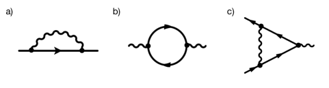
Figure 4: (a) Self-energy, (b) polarization bubble, and (c) vertex correction diagrams in one-loop perturbation theory.

We also point out that since the polarization $\Pi(0,q_{r},q_{z})$ is linear in $\mathbf{q}$ whereas $V(q)\propto 1/q^{2}$, $\Pi$ changes the form of the Coulomb propagator due to screening effects at small $q$,

$$\frac{4\pi e^{2}}{q^{2}-4\pi e^{2}\Pi(0,q_{r}q_{z})}.$$ (120)

For $q\ll\frac{N\alpha}{2\pi^{2}}k_{F}=q_{c}$, Coulomb interactions are screened (although still long range) and the analysis in the vicinity of the fixed point will change. Our analysis indicates that further away from that fixed point, for $q\gtrsim q_{c}$ and $N\alpha<1$, where interactions are unscreened and standard perturbation theory applies, only the velocities run. At low momentum, for $q\ll q_{c}$ and $N\alpha<1$ where interactions are partially screened, no logarithmic divergences are present and the RG flow stops, whereas the charge remains unrenormalized.

C.1 Perturbative RG equations

From Eqs. (117) and (118), the corresponding RG equations for the velocities are:

$$\frac{d\ln v}{d\ell} =\alpha I_{1}(\gamma),$$ (121)

$$\frac{d\ln v_{z}}{d\ell} =\alpha I_{2}(\gamma)$$ (122)

One can equivalently write two equivalent equations,

$$\frac{d\ln\gamma}{d\ell} =\alpha\left[I_{2}(\gamma)-I_{1}(\gamma)\right]\approx\alpha\frac{1-\gamma}{8},$$ (123)

$$\frac{d\ln\alpha}{d\ell} =-\alpha I_{1}(\gamma)\approx-\frac{\alpha}{4}$$ (124)

In this regime, $\alpha$ runs towards an isotropic fixed point with $\alpha=0$ and $\gamma=1$. The solution of the RG equations for $\alpha$ and $\gamma$ is

$$\alpha(\delta k)=\frac{\alpha_{0}}{1+\frac{\alpha_{0}}{4}\ln\left(\frac{\Lambda}{\delta k}\right)},$$ (125)

and

$$\gamma^{-1}(\delta k)=1+\frac{\gamma_{0}^{-1}-1}{\left[1+\frac{\alpha_{0}}{2}\ln\left(\frac{\Lambda}{\delta k}\right)\right]^{\frac{1}{4}}},$$ (126)

while the velocity runs as

$$v(\delta k)=v_{0}\left[1+\frac{\alpha}{4}\ln\left(\frac{\Lambda}{\delta k}\right)\right],$$ (127)

as in graphene (Kotov, ).

Appendix D Derivation of the viscosity in hydrodynamic regime

In a momentum conserved system, the continuity equation for momentum is

$$\frac{\partial\zeta_{j}\left(\mathbf{x},t\right)}{\partial t}+\partial_{i}T_{ij}\left(\mathbf{x},t\right)=0$$ (128)

where $\zeta_{j}\left(x,t\right)$ is the momentum density in space and time $x,t$. Indices $i$, $j$ refer to spatial components in $d$ dimensions. The stress tensor operator $\tau_{ij}$ plays an important role in the transport of viscous quantum fluids. $T_{ij}=-P_{i}\delta_{ij}+T_{ij}^{\prime}$ is composed of pressure $\mathbf{P}$ and of the viscous stress tensor $T_{ij}^{\prime}$, which is the off diagonal part of the stress tensor and can be defined as the expectation of the stress tensor due to strainLandau . In non-equilibrium systems, the deviation in the average stress tensor $\left\langle T_{\mu\nu}^{\prime}\right\rangle$ depends on the strain tensor and its time derivative in linear response,

$$\left\langle T_{ij}^{\prime}\right\rangle=\lambda_{ijk\ell}\xi_{k\ell}+\eta_{ijk\ell}\frac{\partial\xi_{k\ell}}{\partial t}$$ (129)

The component of the viscosity tensor $\eta_{ijk\ell}$ where the component $i=j$ is called bulk viscosity. We are interested in the shear viscosity, where $i\neq j$, so we use $T_{ij}$ and $T_{ij}^{\prime}$ interchangeably. Comparing classical and quantum fluids, there is an analogous relation between the gradients of the velocity field $\mathbf{u}$ and the time derivative of the metric tensor $\xi_{ij}$ (Bradlyn, ):

$$\frac{\partial u_{i}}{\partial x_{j}}=\frac{\partial\xi_{ij}}{\partial t}.$$ (130)

Thus, the shear viscosity can be obtained by the non-equilibrium stress tensor, which is linearized with respect to space derivative of average velocity $\vec{u}$.

To find an effect of strain in the Hamiltonian in linear response, we use the strain generator

$$\mathcal{J}_{ij} =-\frac{1}{2}\sum_{n}\left\{x_{i}^{n},p_{j}^{n}\right\},$$ (131)

where $n$ stands for particle indices. Following Bradlyn and Read’s approach at zero magnetic field (Bradlyn, ), the correction in the Hamiltonian up to first order in $\xi_{\mu\nu}\left(t\right)$ can be shown to be

$$\mathcal{H}_{1}=-\frac{\partial\xi_{ij}}{\partial t}\mathcal{J}_{ij}.$$ (132)

In order to relate the total strain generator $\mathcal{J}_{ij}$ to the energy-stress tensor $\left\langle T_{ij}\right\rangle$, we define the momentum density for a system of $n=1,2,\dots$ particles in the absence of strain as

$$\zeta_{i}\left(\mathbf{x},t\right)=\frac{1}{2}\sum_{n}\left\{p_{i}^{(n)},\delta\left(x_{i}-x_{i}^{(n)}\right)\right\},$$ (133)

and then use the continuity equation (128) in momentum representation,

$$\partial_{t}\zeta_{i}\left(\mathbf{q},t\right)=-iq_{j}\tau_{ij}\left(\mathbf{q},t\right).$$ (134)

Upon expanding the momentum density for small momentum $\mathbf{q}$, we find $\zeta_{i}\left(\mathbf{q},t\right)$ as

$$\zeta_{i}\left(\mathbf{q},t\right) =\int_{\mathbf{x}}e^{i\mathbf{q\cdot x}}\zeta_{i}\left(\mathbf{x},t\right)$$

$$=\zeta_{i}\left(0,t\right)+iq_{j}\frac{1}{2}\sum_{n}\left\{p_{i}^{(n)},x_{j}^{(n)}\right\}+\cdots$$ (135)

where $\zeta_{i}\left(0,t\right)$ is the direct momentum. Hence,

$$\partial_{t}\zeta_{i}\left(\mathbf{q},t\right)-\partial_{t}\zeta_{i}\left(0,t\right)=-\partial_{t}\left[iq_{j}\frac{1}{2}\left\{x_{j},p_{i}\right\}\right]=\partial_{t}iq_{j}\mathcal{J}_{ij}.$$ (136)

If we set $\partial_{t}\zeta_{i}\left(0,t\right)=0$ due to global momentum conservation and compare (134) and (136), the stress tensor is

$$T_{ij}\left(\mathbf{q},t\right)=-\frac{\partial\mathcal{J}_{ij}}{\partial t}.$$ (137)

When we write it in terms of quasiparticle operators,

$$T_{ij}\left(\mathbf{q},t\right) =\sum_{\lambda,a}\int_{\mathbf{k}}\gamma_{\lambda,a}^{\dagger}\left(\mathbf{q}\right)\lambda\frac{\partial}{\partial t}\left(-\mathcal{J}_{ij}\right)\gamma_{\lambda,a}\left(\mathbf{q}\right)$$

$$=\sum_{\lambda,a}\int_{\mathbf{k}}\gamma_{\lambda,a}^{\dagger}\left(\mathbf{q}\right)\frac{\lambda}{2}\frac{\partial}{\partial t}\left(x_{\mu}q_{\nu}+q_{\nu}x_{\mu}\right)\gamma_{\lambda,a}\left(\mathbf{q}\right),$$ (138)

and take the expectation value, then

$$\left\langle T_{\mu\nu}\right\rangle =\sum_{\lambda,a}\int_{\mathbf{k}}\lambda v_{\mu}q_{\nu}\left\langle\gamma_{\lambda,a}^{\dagger}\gamma_{\lambda,a}\right\rangle$$ (139)

$$=N\sum_{\lambda}\int_{\mathbf{k}}v_{\lambda,\mu}q_{\nu}f_{\lambda}\left(k,t\right),$$ (140)

with $N$ being the fermionic degeneracy.

References

- (1) S. Hartnoll, A. Lucas and S. Sachdev, Holographic quantum matter, MIT Press (2016).
- (2) J. Maldacena, The Large N Limit of Superconformal Field Theories and Supergravity, Adv. Theo. Math. Phys. 2, 231 (1998).
- (3) E. Shuryak, Why does the Quark-Gluon Plasma at RHIC behave as a nearly ideal fluid?, Prog. Part. Nucl. Phys. 53, 273 (2004).
- (4) J. Joseph, B. Clancy, L. Luo, J. Kinast, A. Turlapov, and J. E. Thomas, Measurement of Sound Velocity in a Fermi Gas near a Feshbach Resonance, Phys. Rev. Lett. 98, 170401 (2007).
- (5) B. Clancy, L. Luo, and J. E. Thomas, Observation of Nearly Perfect Irrotational Flow in Normal and Superfluid Strongly Interacting Fermi Gases, Phys. Rev. Lett. 99, 140401 (2007).
- (6) P. J. W. Moll, P. Kushwaha, N. Nandi, B. Schmidt, A. P. Mackenzie, Evidence for hydrodynamic electron flow in PdCoO2, Science 351 1061 (2016).
- (7) M. Müller, J. Schmalian, and L. Fritz, Graphene: A Nearly Perfect Fluid, Phys. Rev. Lett. 103, 025301 (2009).
- (8) D. A. Bandurin, I. Torre, R. K. Kumar, M. B. Shalom, A. Tomadin, A. Principi, G. H. Auton, E. Khestanova, K. S. Novoselov, I. V. Grigorieva, L. A. Ponomarenko, A. K. Geim, M. Polini, Negative local resistance caused by viscous electron backflow in graphene, Science 351, 1055 (2016).
- (9) J. Crossno, J. K. Shi, K. Wang, X. Liu, A. Harzheim, A. Lucas, S. Sachdev, P. Kim, T. Taniguchi, K. Watanabe, T. A. Ohki, K. C. Fong, Observation of the Dirac fluid and the breakdown of the Wiedemann-Franz law in graphene, Science, 351, 1058 (2016).
- (10) P. K. Kovtun, D. T. Son, and A. O. Starinets, Viscosity in Strongly Interacting Quantum Field Theories from Black Hole Physics, Phys. Rev. Lett. 94, 111601 (2005).
- (11) M. Shavit, A. Shytov, and Gregory Falkovich, Freely Flowing Currents and Electric Field Expulsion in Viscous Electronics, Phys. Rev. Lett. 123, 026801 (2019).
- (12) A.A. Patel and S. Sachdev, Theory of a Planckian Metal, Phys. Rev. Lett. 123, 066601 (2019).
- (13) J. Zaanen, Y. Liu, Y.-W. Sun and K. Schalm, Holographic duality in condensed matter physics, Cambridge University Press, Cambridge (2015).
- (14) J. Zaanen, Planckian dissipation, minimal viscosity and the transport in cuprate strange metals, SciPost Phys. 6, 061 (2019).
- (15) A.A. Abrikosov and I.M. Khalatnikov, The theory of a fermi liquid (the properties of liquid 3He at low temperatures), Rep. Prog. Phys. 22, 329 (1959).
- (16) M. Brigante, H. Liu, R. C. Myers, S. Shenker, and S. Yaida, Viscosity bound violation in higher derivative gravity, Phys. Rev. D 77, 126006 (2008).
- (17) M. Brigante, H. Liu, R. C. Myers, S. Shenker, and S. Yaida, Viscosity Bound and Causality Violation, Phys. Rev. Lett. 100, 191601 (2008).
- (18) Y. Kats and P. Petrov, Effect of curvature squared corrections in AdS on the viscosity of the dual gauge theory, J. High Energy Phys. 2009, 44 (2009).
- (19) S. A. Hartnoll, D. M. Ramirez, J. E. Santos, Entropy production, viscosity bounds and bumpy black holes, J. High Energy Phys. 2016, 170 (2016).
- (20) L. Alberte, M. Baggioli, O. Pujolàs, Viscosity bound violation in holographic solids and the viscoelastic response, J. High Energy Phys. 2016, 74 (2016).
- (21) M. P. Gochan, H. Li, K. S. Bedell, Viscosity bound violation in viscoelastic Fermi liquids, J. Phys. Comm. 3, 065008 (2019).
- (22) P. Adroguer, D. Carpentier, G. Montambaux, and E. Orignac, Diffusion of Dirac fermions across a topological merging transition in two dimensions, Phys. Rev. B 93, 125113 (2016).
- (23) J. Link, B. N. Narozhny, E. I. Kiselev, and J. Schmalian, Out-of-Bounds Hydrodynamics in Anisotropic Dirac Fluids, Phys. Rev. Lett. 120, 196801 (2018).
- (24) V. N. Kotov, B. Uchoa, O. Sushkov, Coulomb interactions and renormalization of semi-Dirac fermions near a topological Lifshitz transition, Phys. Rev. B 103, 045403 (2021).
- (25) A. A. Burkov, M. D. Hook and L. Balents, Topological nodal semimetals, Phys. Rev. B 84, 235126 (2011).
- (26) K. Mullen, B. Uchoa, D. Glatzhofer, Line of Dirac Nodes in Hyperhoneycomb Lattices, Phys. Rev. Lett. 115, 026403 (2015).
- (27) S. A. Yang, H. Pan, and F. Zhang, Dirac and Weyl Superconductors in Three Dimensions, Phys. Rev. Lett. 113, 046401 (2014).
- (28) Y. Kim, B. J. C. Wieder, C. L. Kane, and A. Rappe, Dirac Line Nodes in Inversion-Symmetric Crystals, Phys. Rev. Lett. 115, 036806 (2015).
- (29) H. Weng, Y. Liang, Q. Xu, Y. Rui, Z. Fang, X. Dai and Y. Kawa, Topological node-line semimetal in three-dimensional graphene networks, Phys. Rev. B 92, 045108 (2015).
- (30) R. Yu, H. Weng, Z. Fang, X. Dai, and X. Hu, Topological Node-Line Semimetal and Dirac Semimetal State in Antiperovskite Cu3PdN, Phys. Rev. Lett. 115, 036807 (2015).
- (31) T. T. Heikkila and G. E. Volovik, Dimensional crossover in topological matter: Evolution of the multiple Dirac point in the layered system to the flat band on the surface, JETP Lett. 93, 59 (2011).
- (32) Y. Chen, Y. Xie, S. A. Yang, H. Pan, F. Zhang, M. L. Cohen, and S. Zhang, Nanostructured Carbon Allotropes with Weyl-like Loops and Points, Nano Letters 15, 6974 (2015).
- (33) L. S. Xie, L. M. Schoop, E. M. Seibel, Q. D. Gibson, W. Xie, and R. J. Cava, Potential ring of Dirac nodes in a new polymorph of Ca3P, APL Mater. 3, 083602 (2015).
- (34) G. Bian, T.-R. Chang, R. Sankar, S-Y. Xu, H. Zheng, T. Neupert, et al., Topological nodal-line fermions in spin-orbit metal PbTaSe2, Nat. Commun. 7, 10556 (2016).
- (35) G. Bian, T.-R. Chang, H. Zheng, S. Velury, S-Y. Xu, T. Neupert, et. al., Drumhead surface states and topological nodal-line fermions in TlTaSe2, Phys. Rev. B 93, 121113(R) (2016).
- (36) B. Song, C. He, S. N., L. Z., Z. Ren, X.-Jun Liu, and G.-B. Jo, Observation of nodal-line semimetal with ultracold fermions in an optical lattice, Nat. Phys. 15, 911 (2019).
- (37) B.-B. Fu, C.-J. Yi, T.-T. Zhang, M. Caputo, J.-Z. Ma, X. Gao, et al., Dirac nodal surfaces and nodal lines in ZrSiS, Sci. Adv. 5, eaau6459 (2019).
- (38) N. E. Hussey, K. Takenaka, H. Takagi, Universality of the Mott–Ioffe–Regel limit in metals, Philos. Mag. 84, 2847 (2004).
- (39) P. Goswami and S. Chakravarty, Quantum Criticality between Topological and Band Insulators in 3 + 1 Dimensions, Phys. Rev. Lett. 107, 196803 (2011).
- (40) P. Hosur, S. A. Parameswaran, and A. Vishwanath, Charge Transport in Weyl Semimetals, Phys. Rev. Lett. 108, 046602 (2012).
- (41) L. Fritz, J. Schmalian, M. Műller, and S. Sachdev, Quantum critical transport in clean graphene, Phys. Rev. B 78, 085416 (2008).
- (42) A. Kashuba, Conductivity of defectless graphene, Phys. Rev. B 78, 085415 (2008).
- (43) For the collisionless conductivity of NLSMs, see S. Ahn, E. J. Mele and H. Min, Electrodynamics on Fermi Cyclides in Nodal Line Semimetals, Phys. Rev. Lett. 119, 147402 (2017); and D. Muñoz-Segovia and A. Cortijo, Many-body effects in nodal-line semimetals: Correction to the optical conductivity, Phys. Rev. B 101, 205102 (2020).
- (44) V. N. Kotov, B. Uchoa, V. M. Pereira, F. Guinea, A. H. Castro Neto, Electron-Electron Interactions in Graphene: Current Status and Perspectives, Rev. Mod. Phys. 84, 1067 (2012).
- (45) Y. Huh, E.-G. Moon, and Y. B. Kim, Long-range Coulomb interaction in nodal-ring semimetals, Phys. Rev. B 93, 035138 (2016).
- (46) Y. Wang and R. M. Nandkishore, Interplay between short-range correlated disorder and Coulomb interaction in nodal-line semimetals, Phys. Rev. B 96, 115130 (2017).
- (47) M. D. Uryszek, F. Krüger, and E. Christou, Fermionic criticality of anisotropic nodal point semimetals away from the upper critical dimension: Exact exponents to leading order in , Phys. Rev. Research 2, 043265 (2020).
- (48) N. Read, Non-Abelian adiabatic statistics and Hall viscosity in quantum Hall states and paired superfluids, Phys. Rev. B 79, 045308 (2009).
- (49) J. E. Avron, R. Seiler, and P. G. Zograf, Viscosity of Quantum Hall Fluids, Phys. Rev. Lett. 75, 697 (1995).
- (50) B. Bradlyn, M. Goldstein, and N. Read, Kubo formulas for viscosity: Hall viscosity, Ward identities, and the relation with conductivity, Phys. Rev. B 86, 245309 (2012).
- (51) L. Levitov and G. Falkovich, Electron viscosity, current vortices and negative nonlocal resistance in graphene, Nat. Phys. 12, 672 (2016).
- (52) C. F. Barenghia, L. Skrbekb, and K. R. Sreenivasan, Introduction to quantum turbulence, Proc. Nat. Acad. Sci. 111, 4647 (2014).
- (53) S. Sur and R. Nandkishore, Instabilities of Weyl loop semimetals, New J. Physics 18, 115006 (2016).
- (54) B. Roy, Interacting nodal-line semimetal: Proximity effect and spontaneous symmetry breaking, Phys. Rev. B 96, 041113(R) (2017).
- (55) A. N. Rudenko, E. A. Stepanov, A. I. Lichtenstein and M. I. Katsnelson, Excitonic Instability and Pseudogap Formation in Nodal Line Semimetal ZrSiS, Phys. Rev. Lett. 120, 216401 (2018).
- (56) J. N. Nelson, J. P. Ruf, Y. Lee, C. Zeledon, J. K. Kawasaki, S. Moser, et al., Dirac nodal lines protected against spin-orbit interaction in IrO2, Phys. Rev. Materials 3, 064205 (2019).
- (57) Y. Shao, et al., Electronic correlations in nodal-line semimetals, Nat. Phys. 16, 636 (2020).
- (58) L. P. Kadanoff, G. Baym, and D. Pines, Quantum statistical mechanics, Originally published in 1962.
- (59) L. D. Landau and E. M. Lifshitz, Fluid Mechanics - 2nd Edition (Pergamon Press, 1987).