Boundary Topological Superconductors

Abstract

For strongly anisotropic time-reversal invariant (TRI) insulators in two and three dimensions, the band inversion can occur respectively at all TRI momenta of a high symmetry axis and plane. Although these classes of materials are topologically trivial as the strong and weak $Z_{2}$ indices are all trivial, they can host an even number of unprotected helical gapless edge states or surface Dirac cones on some boundaries. We show in this work that when the gapless boundary states are gapped by $s_{\pm}$-wave superconductivity, a boundary time-reversal invariant topological superconductor (BTRITSC) characterized by a $Z_{2}$ invariant can be realized on the corresponding boundary. Since the dimension of the BTRITSC is lower than the bulk by one, the whole system is a second-order TRI topological superconductor. When the boundary of the BTRITSC is further cut open, Majorana Kramers pairs and helical gapless Majorana modes will respectively appear at the corners and hinges of the considered sample in two and three dimensions. Furthermore, a magnetic field can gap the helical Majorana hinge modes of the three-dimensional second-order TRI topological superconductor and lead to the realization of a third-order topological superconductor with Majorana corner modes. Our proposal can potentially be realized in insulator-superconductor heterostructures and iron-based superconductors whose normal states take the desired inverted band structures.

Topological insulators (TIs) and topological superconductors (TSCs) are two classes of materials which have a nontrivial gapped band structure in the bulk and novel gapless excitations on the boundaryHasan and Kane (2010); Qi and Zhang (2011). The band topology of TIs with time-reversal symmetry is known to be characterized by a $Z_{2}$ invariant $\nu$ in two dimensions (2D) and four $Z_{2}$ invariants $(\nu_{0};\nu_{1}\nu_{2}\nu_{3})$ in 3DKane and Mele (2005); Fu et al. (2007); Moore and Balents (2007); Roy (2009); Fu and Kane (2007). If the inversion symmetry is also preserved, these $Z_{2}$ invariants can be simply inferred from the parity eigenvalues at time-reversal invariant (TRI) momentaFu and Kane (2007), or equivalently, the number and distribution of TRI momenta at which the band inversion occurs. In 2D, when the band inversion occurs at an odd number of TRI momenta, $\nu$ is necessitated to take the nontrivial value, and a TI with an odd number of helical gapless states on each edge is realizedKönig et al. (2007); Knez et al. (2011); Wu et al. (2018). Similarly, when the band inversion occurs at an odd number of TRI momenta in 3D, the strong $Z_{2}$ index $\nu_{0}$ is also necessitated to take the nontrivial value, and a strong TI with an odd number of Dirac cones on each surface is realizedZhang et al. (2009); Chen et al. (2009); Xia et al. (2009); Hsieh et al. (2009a). In contrast, when the band inversion occurs at an even number of TRI momenta, the strong $Z_{2}$ index is trivial, but some of the three weak indices $(\nu_{1}\nu_{2}\nu_{3})$ can still be nontrivial. For instance, when the band inversion occurs at $2$ (mod $4$) TRI momenta, at least one of $(\nu_{1}\nu_{2}\nu_{3})$ must be nontrivial according to their definitionFu and Kane (2007), leading to the realization of a weak TI in which the surface Dirac cones only appear selectively on certain surfaces and their number on each surface is even rather than oddLiu et al. (2016); Noguchi et al. (2019).

Because of the time-reversal symmetry, the gapless boundary states in TIs are spin-momentum-lockedHsieh et al. (2009b). Remarkably, this property allows the establishment of a direct connection between TIs and TSCs. In the pioneering work of Fu and KaneFu and Kane (2008), it was shown that when the gapless surface Dirac cones of a strong TI are gapped by $s$-wave superconductivity, topological superconductivity can be realized in the $\pi$-flux vortices, manifested by the presence of Majorana zero modes (MZMs). The vortex MZMs also follow a $Z_{2}$ classification, which means that there exists one topologically protected MZM only when the number of MZMs in a $\pi$-flux vortex is oddHosur et al. (2011); Qin et al. (2019); Yan et al. (2020). On the other hand, the number of MZMs is directly connected to the number of surface Dirac cones, therefore, insulators with an even number of band inversions are disfavored in this scenario. Apparently, this rules out a considerable amount of strongly anisotropic materials which generally favor an even number of band inversions.

In this work, we build a new scenario which favors such strongly anisotropic band-inverted insulators. Concretely, we consider insulators with both time-reversal symmetry and inversion symmetry, whose band inversions occur at all TRI momenta of a high symmetry axis in 2D and a high symmetry plane in 3D. Although such band-inverted insulators are topologically trivial as the strong and weak $Z_{2}$ indices are all trivial, they can host an even number of unprotected helical gapless edge states in 2D and surface Dirac cones in 3D on some boundaries. The gapless boundary states are found to form floating bands which are non-degenerate due to the breaking of inversion symmetry on the boundary. By introducing $s_{\pm}$-wave superconductivity rather than $s$-wave superconductivity to gap the gapless floating bands, we find that a TRI TSC characterized by a $Z_{2}$ invariant can be realized on the corresponding boundary, even though the band topology of the bulk is necessitated to be trivial. As the TRI TSC is realized on the boundary, we term it boundary time-reversal invariant topological superconductor (BTRITSC). Because the dimension of the BTRITSC is lower than the bulk by one, the whole system is a second-order TRI TSC which harbors Majorana Kramers pairs (two MZMs related by time-reversal symmetry) at the sample corners in 2D and helical gapless Majorana modes at the sample hinges in 3DYan et al. (2018); Wang et al. (2018a); Zhang et al. (2019a); Gray et al. (2019); Hsu et al. (2020); Vu et al. (2020); Wu et al. (2020a). Remarkably, a magnetic field can gap the helical Majorana hinge modes in 3D and lead to the realization of a third-order TSC with Majorana corner modesYan (2019a); Ahn and Yang (2020). The new scenario thus unveils a new route for the realization of higher-order TSCsLangbehn et al. (2017); Shapourian et al. (2018); Khalaf (2018); Geier et al. (2018); Zhu (2018); Wang et al. (2018b); Hsu et al. (2018); Liu et al. (2018a); Wu et al. (2019); Volpez et al. (2019); Zhang et al. (2019b); Wu et al. (2019); Zeng et al. (2019); Bultinck et al. (2019); Ghorashi et al. (2019); Peng and Xu (2019); Zhu (2019); Laubscher et al. (2019); Pan et al. (2019); Yan (2019b); Franca et al. (2019); Kheirkhah et al. (2020a); Zhang and Trauzettel (2020); Roy (2020); Wu et al. (2020b); Kheirkhah et al. (2020b); Wu et al. (2020c); Tiwari et al. (2020); Ono et al. (2020a, b).

BTRITSCs in 2D.— To illustrate the essential physics, we start with a simple 2D Bogoliubov-de Gennes (BdG) Hamiltonian $H=\frac{1}{2}\sum_{\boldsymbol{k}}\psi_{\boldsymbol{k}}^{{\dagger}}H_{\rm BdG}(\boldsymbol{k})\psi_{\boldsymbol{k}}$, where

$$H_{\rm BdG}(\boldsymbol{k}) = \left(\begin{array}[]{cc}H_{0}(\boldsymbol{k})-\mu\Sigma_{00}&-i\Sigma_{20}\Delta(\boldsymbol{k})\\ i\Sigma_{20}\Delta(\boldsymbol{k})&\mu\Sigma_{00}-H_{0}^{*}(-\boldsymbol{k})\\ \end{array}\right),$$ (3)

$$H_{0}(\boldsymbol{k}) = \epsilon_{\rm 2D}(\boldsymbol{k})\Sigma_{00}+m_{\rm 2D}(\boldsymbol{k})\Sigma_{03}+\lambda_{1}\sin k_{1}\Sigma_{31}$$

$$+\lambda_{2}\sin k_{2}\Sigma_{02},$$

$$\Delta(\boldsymbol{k}) = \Delta_{0}-\Delta_{1}(\cos k_{1}+\cos k_{2}),$$ (4)

and $\psi_{\boldsymbol{k}}=(c_{\boldsymbol{k},a,\uparrow},c_{\boldsymbol{k},b,\uparrow},c_{\boldsymbol{k},a,\downarrow},c_{\boldsymbol{k},b,\downarrow},c_{-\boldsymbol{k},a,\uparrow}^{{\dagger}},c_{-\boldsymbol{k},b,\uparrow}^{{\dagger}},c_{-\boldsymbol{k},a,\downarrow}^{{\dagger}},\\ c_{-\boldsymbol{k},b,\downarrow}^{{\dagger}})^{T}$. In the BdG Hamiltonian (4), $\Sigma_{ij}=s_{i}\otimes\sigma_{j}$, where the Pauli matrices $s_{i}$ and $\sigma_{j}$ act respectively on the spin $(\uparrow,\downarrow)$ and orbital $(a,b)$ degrees of freedom, and $s_{0}$ and $\sigma_{0}$ are $2\times 2$ unit matrices. $H_{0}(\boldsymbol{k})$ describes the normal state, with the first term characterizing the asymmetry of the conduction and valence bands, the second term characterizing the band inversion, and the last two terms representing spin-orbit coupling. Here we take $\epsilon_{\rm 2D}(\boldsymbol{k})=\epsilon_{1}\cos k_{1}+\epsilon_{2}\cos k_{2}$, $m_{\rm 2D}(\boldsymbol{k})=m_{0}-m_{1}\cos k_{1}-m_{2}\cos k_{2}$, and $\lambda_{1,2}$ are assumed to be positive. $\Delta(\boldsymbol{k})$ describes the superconducting order parameter. In this work, we consider $s_{\pm}$-wave superconductivity which can be achieved intrinsicallyWang et al. (2015); Wu et al. (2016); Xu et al. (2016); Zhang et al. (2018); Wang et al. (2018c); Kong et al. (2019); Machida et al. (2019); Liu et al. (2018b); Chen et al. (2019); Zhu et al. (2020) or extrinsically by superconducting proximity effect from an iron-based superconductorMazin et al. (2008); Wang and Lee (2011). Moreover, the lattice constants are set to unity throughout for notational simplicity.

It is readily verified that $H_{0}$ has both time-reversal symmetry and inversion symmetry, with the time-reversal and inversion operators given by $T=is_{2}\otimes\sigma_{0}\mathcal{K}$ and $P=s_{0}\otimes\sigma_{3}$, respectively, where $\mathcal{K}$ denotes the complex conjugation. Accordingly, the bulk bands have Kramers degeneracy at every momentum, and the $Z_{2}$ invariant characterizing the band topology of $H_{0}(\boldsymbol{k})$ is simply given byFu and Kane (2007)

$$(-1)^{\nu}=\prod_{i=1}^{4}\xi(\mathbf{\Gamma_{i}}),$$ (5)

where $\xi(\mathbf{\Gamma_{i}})$ denotes the parity eigenvalue of the two lower Kramers degenerate bands at the TRI momenta $\mathbf{\Gamma_{i}}$ ($\mathbf{\Gamma_{i}}=-\mathbf{\Gamma_{i}}$ up to a reciprocal lattice vector). For $H_{0}(\boldsymbol{k})$, it is readily found that away from the critical lines $m_{0}\pm m_{1}\pm m_{2}=0$ where the bulk gap gets closed, we have

$$(-1)^{\nu}=\prod_{\alpha=\pm 1,\beta=\pm 1}\text{sgn}(m+\alpha m_{1}+\beta m_{2}).$$ (6)

According to the above formula, the phase diagram can be straightforwardly determined, as shown in Fig.1(a). In the phase diagram, the normal (or trivial) insulator (NI) phase is further divided into two distinct parts. The first part labeled as NI₁ has zero (mod $4$) band inversion (or equivalently to say, the parity eigenvalues at the four TRI momenta take the same sign in these regimes), and the second part labeled as NI₂ has band inversions at two TRI momenta. We are interested in NI₂ since gapless boundary states can appear on certain boundaries, whereas they are completely absent in NI₁.

In the following, we consider a specific case where the band inversion occurs at the two TRI momenta $(k_{1},k_{2})=(0,0)$ and $(\pi,0)$ to illustrate the essential physics. Without loss of generality, we take $m_{1}=1$ as the energy unit and set $m_{0}=0$ and $m_{2}=2$ to realize the desired condition. To reveal the selective existence of helical gapless states on certain boundaries, we consider that the insulator takes a cylinder geometry with open boundary condition in one direction and periodic boundary condition in the other orthogonal direction. The results shown in Figs.1(b)(c) indicate that helical gapless states do not appear on the $x_{1}$-normal edges, but appear on the $x_{2}$-normal edges. One can see that the helical edge states cross at both TRI momenta in the edge Brillouin zone, suggesting the presence of two pairs of helical gapless states on each $x_{2}$-normal edge. However, unlike TIs, the helical gapless edge states do not traverse the bulk gap, instead they form two floating bands within the gap. It is noteworthy that conduction-valence asymmetry only affects the dispersion of the floating bands. The floating bands exist even if the asymmetry is strong enough to change the insulator to a metal, as shown in Fig.1(d).

Figure 1: (a) Phase diagram of the normal state. (b)(c)(d) Energy spectrum under a cylinder geometry. The lattice size along the direction with open boundary condition is $L=100$. (b) No gapless state appears on the $x_{1}$-normal edges. (c) The in-gap dispersions (blue lines) are of double degeneracy, corresponding to the presence of two pairs of helical gapless states on each $x_{2}$-normal edge. The helical gapless states on each edge form two non-degenerate floating bands. (d) The floating bands remain in the gap even when the conduction-valence asymmetry is strong enough to change the insulator to a metal. Common parameters are $m_{1}=1$, $m_{0}=0$, $m_{2}=2$, $\lambda_{1}=0.5$, $\lambda_{2}=1$. $\epsilon_{1,2}=0$ in (b) (c), and $\epsilon_{1}=0$, $\epsilon_{2}=1.5$ in (d).

Let us now take into account the $s_{\pm}$-wave superconductivity. Before focusing on the boundary, we first discuss the bulk. As the TRI BdG Hamiltonian belongs to the DIII class, the band topology of its 2D bulk also follows a $Z_{2}$ classificationSchnyder et al. (2008); Kitaev (2009); Haim and Oreg (2019). For the concerned spin-singlet pairing, the $Z_{2}$ invariant is simply given byQi et al. (2010)

$$N_{\rm 2D}=\prod_{s}[\text{sgn}(\Delta_{s})]^{m_{s}},$$ (7)

where $m_{s}$ denotes the number of TRI momenta enclosed by the $s$th Fermi surface, and $\text{sgn}(\Delta_{s})$ denotes the sign of the pairing on the $s$th Fermi surface. Because the normal state has both time-reversal symmetry and inversion symmetry, the Kramers degeneracy at every momentum forces the double degeneracy of Fermi surface, if any. As a result, $N_{\rm 2D}$ is necessitated to take the trivial value $1$. Therefore, the bulk is always topologically trivial for the concerned spin-singlet pairing. However, the inversion symmetry is broken on the boundary, which consequently lifts the Kramers degeneracy. Indeed, on each $x_{2}$-normal edge, the floating bands shown in Figs.1(c)(d) do not have Kramers degeneracy away from the two TRI momenta, which, as will be shown in the following, enables the realization of 1D TRI TSC on the boundary.

As the floating bands extends over the whole Brillouin zone, they can be described by a truly 1D lattice Hamiltonian. This is sharply distinct to 2D TIs in which a lattice realization of the helical gapless edge states is known to be impossible. Without loss of generality, we take the simple conduction-valence symmetric case for illustration. In this limit, the floating bands shown in Fig.1(c) on one of the $x_{2}$-normal edges is simply described by

$$H_{f}(k_{1})=\lambda_{1}\sin k_{1}s_{3}.$$ (8)

In the presence of $s_{\pm}$-wave superconductivity, the BdG Hamiltonian on the corresponding edge reads

$$H_{\rm e}(k_{1}) = \lambda_{1}\sin k_{1}\tau_{0}\otimes s_{3}-\mu\tau_{3}\otimes s_{0}$$ (9)

$$+(\Delta_{0}-\Delta_{1}\cos k_{1}-\Delta_{2}(k_{1}))\tau_{2}\otimes s_{2},$$

where the Pauli matrices $\tau_{i}$ act on the particle-hole space, and $\Delta_{2}(k_{1})\simeq\Delta_{1}(m_{0}-m_{1}\cos k_{1})/m_{2}$ (here we provide a general expression), which is originated from the $\Delta_{1}\cos k_{2}$ term of the pairing under the open boundary condition in the $x_{2}$ direction (see details in the Supplemental Materialsup ). This 1D TRI BdG Hamiltonian also follows a $Z_{2}$ classification and the $Z_{2}$ invariant takes a form similar to Eq.(7)Qi et al. (2010),

$$N_{\rm 1D}=\prod_{s}[\text{sgn}(\Delta_{s})],$$ (10)

where $\text{sgn}(\Delta_{s})$ denotes the sign of the pairing on the $s$th Fermi point between $0$ and $\pi$, as illustrated in Fig.2(a). According to Eq.(9), there are two Fermi points between $0$ and $\pi$ when $\mu\in(-\lambda_{1},\lambda_{1})$, which are located at $k_{s,a}=\arcsin(|\mu/\lambda_{1}|)$ and $k_{s,b}=\pi-k_{s,a}$. Following Eq.(10), we then have

$$N_{\rm 1D}=\text{sgn}[(\Delta_{0}-\frac{m_{0}\Delta_{1}}{m_{2}})^{2}-\Delta_{1}^{2}(1-\frac{m_{1}}{m_{2}})^{2}(1-\frac{\mu^{2}}{\lambda_{1}^{2}})^{2}]\,$$ (11)

in the regime $\mu\in(-\lambda_{1},\lambda_{1})$. Under appropriate condition, $N_{\rm 1D}$ can take the nontrivial value $-1$, which corresponds to the realization of a 1D BTRITSC. It is noteworthy that when $\mu^{2}>\lambda_{1}^{2}$, there is no Fermi point, so $N_{\rm 1D}$ always takes the trivial value $1$, indicating a trivial boundary.

Figure 2: (a) The sign of pairing on the Fermi points between $0$ and $\pi$. The two solid black lines denote the floating bands formed by the gapless boundary states. The dashed blue line denotes the Fermi level, and the two dashed purple lines indicate the momenta at which the pairing changes sign. The blue and red star denote the Fermi points with negative and positive pairing, respectively. (b) Density profiles of four Majorana Kramers pairs are located at the four corners of the considered square sample. The inset shows a few energy eigenvalues closest to zero. The parameters in (a) and (b) are $m_{0}=0$, $m_{1}=1$, $m_{2}=2$, $\lambda_{1}=0.5$, $\lambda_{2}=1.0$, $\epsilon_{1,2}=0$, $\Delta_{1}=0$, $\Delta_{1}=0.2$.

To further demonstrate the above analytical results, we consider $\{m_{0},m_{1},m_{2},\Delta_{0},\Delta_{1}\}=\{0,1,2,0,0.2\}$. Then according to Eq.(11), we have $N_{\rm 1D}=-1$ in the regime $\mu\in(-\lambda_{1},\lambda_{1})$. As a 1D TRI TSC is characterized by the existence of one Majorana Kramers pair on each endWong and Law (2012); Zhang et al. (2013); Keselman et al. (2013); Haim et al. (2014); Gaidamauskas et al. (2014); Schrade et al. (2015), the realization of BTRITSCs will be manifested by the presence of Majorana Kramers pairs at the boundary of the BTRITSCs, i.e., the corners of a square sample. As shown in Fig.2(b), the numerical result confirms the prediction. It is noteworthy that from a bulk perspective, the presence of Majorana Kramers pairs at the corners indicates that the whole system is a second-order TRI TSCYan et al. (2018); Wang et al. (2018a).

BTRITSCs in 3D.— The generalization to 3D is straightforward. We only need to generalize the normal-state Hamiltonian into a 3D form and keep the pairing term intact. Here we consider

$$H_{0}(\boldsymbol{k}) = \epsilon_{\rm 3D}(\boldsymbol{k})\Sigma_{00}+m_{\rm 3D}(\boldsymbol{k})\Sigma_{03}+\sum_{i}\lambda_{i}\sin k_{i}\Sigma_{i1},$$ (12)

where $\epsilon_{\rm 3D}(\boldsymbol{k})=\sum_{i}\epsilon_{i}\cos k_{i}$ and $m_{\rm 3D}(\boldsymbol{k})=m_{0}-\sum_{i}m_{i}\cos k_{i}$ ($i$ runs over $1$, $2$ and $3$). Similarly, without loss of generality, we consider that the band inversion occurs at the four TRI momenta of the $k_{3}=0$ plane. For such a configuration, both the strong and weak $Z_{2}$ indices are trivial because the product of parity eigenvalues in each of the $k_{1,2,3}=0/\pi$ planes gives the trivial valueFu and Kane (2007). To realize this configuration, we take $m_{0}=0$, $m_{1}=m_{2}=1$ and $m_{3}=3$. As shown in Fig.3(a), this configuration realizes 2D spin-degeneracy-lifted floating bands on the $x_{3}$-normal surfaces. By performing similar analysis as in 2D, we find that the floating bands of the normal state are described by

$$H_{f}(k_{1},k_{2})=\lambda_{1}\sin k_{1}s_{1}+\lambda_{2}\sin k_{2}s_{2}.$$ (13)

In the presence of $s_{\pm}$-wave superconductivity, the corresponding surface BdG Hamiltonian takes a very simple form, which reads

$$H_{\rm s}(k_{1},k_{2}) = \lambda_{1}\sin k_{1}\tau_{0}\otimes s_{1}+\lambda_{2}\sin k_{2}\tau_{3}\otimes s_{2}-\mu\tau_{3}\otimes s_{0}$$ (14)

$$+(\Delta_{0}-\Delta_{1}(\cos k_{1}+\cos k_{2}))\tau_{2}\otimes s_{2}.$$

The band topology of $H_{\rm s}$ is just characterized by the $Z_{2}$ invariant given in Eq.(7). As the normal-state Fermi surface is determined by $\pm\sqrt{\sum_{j=1,2}\lambda_{j}^{2}\sin^{2}k_{j}}=\mu$, and the pairing changes sign at the nodal line determined by $\Delta_{0}-\Delta_{1}(\cos k_{1}+\cos k_{2})=0$, $N_{\rm 2D}$ can be intuitively determined by inspecting the configuration of Fermi surface and pairing nodal line, as illustrated in Fig.3(b). When the pairing nodal line encloses one Fermi surface, $N_{\rm 2D}=-1$, and a 2D BTRITSC is realized. Similarly, the realization of a 2D BTRITSC is manifested by the presence of helical Majorana modesDeng et al. (2012); Zhang et al. (2013), as shown in Figs.3(c)(d). As the helical Majorana modes appear at the boundary of the $z$-normal surfaces, the whole system is a 3D second-order TRI TSC from a bulk perspectiveZhang et al. (2019a).

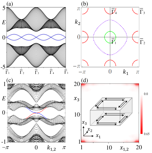
Figure 3: (a) Normal-state energy spectrum for a geometry with open boundary condition in the $x_{3}$ direction and periodic boundary condition in the $x_{1}$ and $x_{2}$ directions. The spectrum is shown along the high symmetric lines of the surface Brillouin zone. (b) A configuration with $N_{\rm 2D}=-1$. The dashed purple line denotes the pairing nodal line, and the solid red and green lines on its two sides denote Fermi surfaces with positive and negative pairing, respectively. (c) Superconducting-state energy spectrum for the configuration in (b). The sample takes open boundary condition in the $x_{1}(x_{2})$ and $x_{3}$ directions and periodic boundary condition in the $x_{2}(x_{1})$ direction. Because the Hamiltonian has $C_{4}$ rotation symmetry, the energy spectra for the two cases are the same. The in-gap dispersions are of four-fold degeneracy, which correspond to four pairs of helical Majorana modes. (d) The density profiles of the helical Majorana modes are localized at the hinges of the sample. The inset provides an intuitive illustration of their distribution on the cubic sample. Common parameters are $\epsilon_{1,2,3}=0$, $m_{0}=0$, $m_{1,2}=1$, $m_{3}=3$, $\lambda_{1,2}=0.5$, $\lambda_{3}=1.5$. In (b)(c)(d), $\Delta_{0}=0.1$, $\Delta_{1}=0.15$ and $\mu=0.3$.

Effect of an external magnetic field.— Thus far, the time-reversal symmetry, which prohibits two time-reversal partner Majorana modes from coupling, has been assumed to be preserved. Applying a magnetic field will generate a Zeeman term of the form $(B_{1}\tau_{0}\otimes s_{1}+B_{2}\tau_{3}\otimes s_{2}+B_{3}\tau_{0}\otimes s_{3})\otimes\sigma_{0}$, accordingly breaking this symmetry. Although the Majorana Kramers pairs in 2D and helical Majorana hinge modes in 3D are no longer protected when the time-reversal symmetry is broken, the magnetic field can induce interesting topological phase transitions. In 2D, the Majorana Kramers pairs can be changed to solitary MZMs when the magnetic field exceeds a critical valueYan et al. (2018). Remarkably, in 3D, a magnetic field in the $x_{1}$-$x_{2}$ plane can immediately gap the helical Majorana hinge modes and lead to the presence of solitary MZMs at certain inversion-related cornersZhu (2018); Volpez et al. (2019). It means that the magnetic field can change the second-order TRI TSC to a third-order time-reversal-symmetry-breaking TSCYan (2019a); Ahn and Yang (2020). It is noteworthy that such a response to magnetic field is sharply distinct to second-order TRI TSCs realized by a combination of strong TIs and $s_{\pm}$-wave superconductivityZhang et al. (2019a); Kheirkhah et al. (2020c). For the latter, counter-intuitively, the magnetic field cannot gap the helical Majorana hinge modes, because they have a domain-wall origin therein and the magnetic field cannot directly act on the domain-wall subspaceKheirkhah et al. (2020c).

Conclusions.— In this work, we have shown that 1D and 2D TRI TSCs can be respectively realized on the boundary of 2D and 3D trivial band-inverted insulators when their unprotected gapless boundary states are gapped by $s_{\pm}$-wave superconductivity. Because the dimension of the BTRITSCs is lower than the bulk by one, the BTRITSCs open a new route for the realization of second-order TRI TSCs. In addition, we found that by applying a magnetic field, a third-order TSC with Majorana corner modes can be readily induced from the second-order TRI TSC realized in this route. Our established new scenario unveils that the widely-overlooked trivial band-inverted insulators can also be applied for the realization of TSCs and concomitant Majorana modes, hopefully broadening the scope of material candidates for TSCs.

Acknowledgements.— This work is supported by the Startup Grant (No. 74130- 18841219) and the National Science Foundation of China (Grant No. 11904417).

This supplemental material contains the derivation of boundary Hamiltonians. We start with the normal-state Hamiltonian in two dimensions (2D), which is given by

$$H_{0}(\boldsymbol{k}) = (\epsilon_{1}\cos k_{1}+\epsilon_{2}\cos k_{2})\Sigma_{00}+(m_{0}-m_{1}\cos k_{1}-m_{2}\cos k_{2})\Sigma_{03}$$ (S1)

$$+\lambda_{1}\sin k_{1}\Sigma_{31}+\lambda_{2}\sin k_{2}\Sigma_{02},$$

where $\Sigma_{ij}=s_{i}\otimes\sigma_{j}$, with the Pauli matrices $s_{i}$ and $\sigma_{j}$ acting respectively on the spin $(\uparrow,\downarrow)$ and orbital $(a,b)$ degrees of freedom. $s_{0}$ and $\sigma_{0}$ are two-by-two unit matrices.

Consider that the band inversion occurs at the two time-reversal invariant (TRI) momenta $(k_{1},k_{2})=(0,0)$ and $(\pi,0)$, we first make a Taylor expansion around $k_{2}=0$ to the second order of $k_{2}$. Accordingly, we have

$$H_{0}(k_{1},k_{2})=[\epsilon(k_{1})-\frac{\epsilon_{2}}{2}k_{2}^{2}]\Sigma_{00}+[m(k_{1})+\frac{m_{2}}{2}k_{2}^{2}]\Sigma_{03}+\lambda_{1}\sin k_{1}\Sigma_{31}+\lambda_{2}k_{2}\Sigma_{02},$$ (S2)

where $\epsilon(k_{1})=\epsilon_{2}+\epsilon_{1}\cos k_{1}$ and $m(k_{1})=m_{0}-m_{2}-m_{1}\cos k_{1}$. In the following, we consider $m_{2}$ and $\lambda_{2}$ to be positive. According to the band inversion, we have $m(k_{1})<0$ for an arbitrary $k_{1}\in(-\pi,\pi)$.

To obtain the gapless states on the $x_{2}$-normal edges, we further consider a half-infinity sample which occupies the region $0\leq x_{2}\leq+\infty$. Because the translational symmetry is broken in the $x_{2}$ direction, the wave vector $k_{2}$ needs to be replaced by $-i\partial_{x_{2}}$. Accordingly, the Hamiltonian becomes

$$H_{0}(k_{1},-i\partial_{x_{2}}) = [\epsilon(k_{1})+\frac{\epsilon_{2}}{2}\partial_{x_{2}}^{2}]\Sigma_{00}+[m(k_{1})-\frac{m_{2}}{2}\partial_{x_{2}}^{2}]\Sigma_{03}$$ (S3)

$$+\lambda_{1}\sin k_{1}\Sigma_{31}-i\lambda_{2}\partial_{x_{2}}\Sigma_{02}.$$

Next, we divide the Hamiltonian into two parts, i.e., $H_{0}=H_{1}+H_{2}$, where

$$H_{1}(k_{1},-i\partial_{x_{2}}) = [m(k_{1})-\frac{m_{2}}{2}\partial_{x_{2}}^{2}]\Sigma_{03}-i\lambda_{2}\partial_{x_{2}}\Sigma_{02},$$

$$H_{2}(k_{1},-i\partial_{x_{2}}) = [\epsilon(k_{1})+\frac{\epsilon_{2}}{2}\partial_{x_{2}}^{2}]\Sigma_{00}+\lambda_{1}\sin k_{1}\Sigma_{31}.$$ (S4)

We first solve the eigenvalue equation $H_{1}(k_{1},-i\partial_{x_{2}})\psi(x_{2})=E\psi(x_{2})$ under the boundary condition $\psi(0)=\psi(+\infty)=0$. It is readily found that there are two zero-energy solutions for an arbitrary $k_{1}\in(-\pi,\pi)$. The two solutions take the form

$$\psi_{\alpha=1,2}(x_{2})=\mathcal{N}\sin(\kappa_{1}x_{2})e^{-\kappa_{2}x_{2}}e^{ik_{1}x_{1}}\chi_{\alpha},$$ (S5)

with normalization given by $|\mathcal{N}|^{2}=4|\kappa_{2}(\kappa_{1}^{2}+\kappa_{2}^{2})/\kappa_{1}^{2}|$, where $\kappa_{1}=\sqrt{-\frac{2m(k_{1})}{m_{2}}-\frac{\lambda_{2}^{2}}{m_{2}^{2}}}$, and $\kappa_{2}=\frac{\lambda_{2}}{m_{2}}$. Furthermore, $\chi_{\alpha}$ satisfy $\Sigma_{01}\chi_{\alpha}=\chi_{\alpha}$, which can be chosen as

$$\chi_{1} = |s_{3}=1,\sigma_{1}=1\rangle,$$

$$\chi_{2} = |s_{3}=-1,\sigma_{1}=1\rangle.$$ (S6)

By projecting $H_{2}$ into the subspace expanded by $\chi_{1}$ and $\chi_{2}$, we obtain the boundary Hamiltonian, which is given by

$$[H_{e}(k_{1})]_{\alpha\beta} = \int_{0}^{+\infty}dx_{2}\psi_{\alpha}^{{\dagger}}(x_{2})H_{2}(k_{1},-i\partial_{x_{2}})\psi_{\beta}(x_{2})$$ (S7)

$$= \left\{[\epsilon(k_{1})+\frac{m_{1}(k_{1})\epsilon_{2}}{m_{2}}]s_{0}+\lambda_{1}\sin k_{1}s_{3}\right\}_{\alpha\beta},$$

or equivalently,

$$H_{e}(k_{1}) = [\epsilon(k_{1})+\frac{m_{1}(k_{1})\epsilon_{2}}{m_{2}}]s_{0}+\lambda_{1}\sin k_{1}s_{3}$$ (S8)

$$= [\frac{m_{0}\epsilon_{2}}{m_{2}}+\epsilon_{1}\cos k_{1}-\frac{m_{1}\epsilon_{2}}{m_{2}}\cos k_{1}]s_{0}+\lambda_{1}\sin k_{1}s_{3}.$$

For the conduction-valence symmetric case, i.e., $\epsilon_{1,2}=0$, Eq.(S8) reduces to Eq.(8) of the main text, and the analytical results perfectly agree with the numerical results, as shown in Fig.S1(a). When conduction-valence asymmetry is present and strong, the analytical results still agree with the numerical results well, as shown in Figs.S1(b)(c).

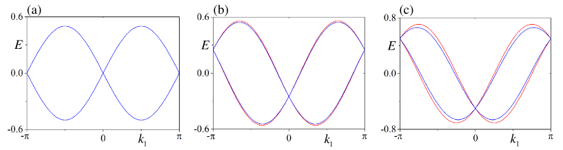
Figure S1: Dispersions of the helical gapless states on the $x_{2}$-normal edges. The blue curves correspond to numerical results, and the red curves correspond to analytical results. (a) $\epsilon_{1}=\epsilon_{2}=0$, the numerical and analytical results perfectly agree with each other. (b) $\epsilon_{1}=0$, $\epsilon_{2}=0.5$, the numerical and analytical results show small deviation away from time-reversal invariant momenta. (c) $\epsilon_{1}=0$, $\epsilon_{2}=1$. The increase of conduction-valence asymmetry increases the deviation between numerical and analytical results, suggesting that the expansion of $k_{2}$ to the second order is no longer sufficient.

After taking into account the $s_{\pm}$-wave pairings, the Hamiltonian needs to be generalized as

$$H_{\rm BdG}(\boldsymbol{k}) = [(\epsilon_{1}\cos k_{1}+\epsilon_{2}\cos k_{2})-\mu]\Sigma_{300}+(m_{0}-m_{1}\cos k_{1}-m_{2}\cos k_{2})\Sigma_{303}$$ (S9)

$$+\lambda_{1}\sin k_{1}\Sigma_{031}+\lambda_{2}\sin k_{2}\Sigma_{302}+[\Delta_{0}-\Delta_{1}(\cos k_{1}+\cos k_{2})]\Sigma_{220}.$$

where $\Sigma_{ijk}=\tau_{i}\otimes s_{j}\otimes\sigma_{k}$, with the new Pauli matrices $\tau_{i}$ acting on the particle-hole degrees of freedom. Similarly, we make an expansion about $k_{2}$, and then do the replacement $k_{2}\rightarrow-i\partial_{x_{2}}$ and decomposition $H_{\rm BdG}=H_{1}+H_{2}$. Accordingly, we have

$$H_{1}(k_{1},-i\partial_{x_{2}}) = [m(k_{1})-\frac{m_{2}}{2}\partial_{x_{2}}^{2}]\Sigma_{303}-i\lambda_{2}\partial_{x_{2}}\Sigma_{302},$$

$$H_{2}(k_{1},-i\partial_{x_{2}}) = [\epsilon(k_{1})+\frac{\epsilon_{2}}{2}\partial_{x_{2}}^{2}-\mu]\Sigma_{300}+\lambda_{1}\sin k_{1}\Sigma_{031}+[\Delta_{0}-\Delta_{1}\cos k_{1}-(\Delta_{1}+\frac{\Delta_{1}}{2}\partial_{x_{2}}^{2})]\Sigma_{220}.$$ (S10)

Because of the increase of particle-hole degrees of freedom, now there are four zero-energy solutions of the eigenvalue equation $H_{1}(k_{1},-i\partial_{x_{2}})\psi_{\alpha}(x_{2})=E\psi_{\alpha}(x_{2})$. The general form of $\psi_{\alpha}(x_{2})$ still reads

$$\psi_{\alpha=1,2,3,4}(x_{2})=\mathcal{N}\sin(\kappa_{1}x_{2})e^{-\kappa_{2}x_{2}}e^{ik_{1}x_{1}}\chi_{\alpha},$$ (S11)

but now $\chi_{\alpha}$ satisfy $\Sigma_{001}\chi_{\alpha}=\chi_{\alpha}$, which can be chosen as

$$\chi_{1} = |\tau_{3}=1,s_{3}=1,\sigma_{1}=1\rangle,$$

$$\chi_{2} = |\tau_{3}=1,s_{3}=-1,\sigma_{1}=1\rangle,$$

$$\chi_{3} = |\tau_{3}=-1,s_{3}=1,\sigma_{1}=1\rangle,$$

$$\chi_{4} = |\tau_{3}=-1,s_{3}=-1,\sigma_{1}=1\rangle.$$ (S12)

By projecting $H_{2}$ into the four-dimensional subspace expanded by $\chi_{1,2,3,4}$, we obtain the boundary Hamiltonian, which is given by

$$[H_{e}(k_{1})]_{\alpha\beta} = \int_{0}^{+\infty}dx_{2}\psi_{\alpha}^{{\dagger}}(x_{2})H_{2}(k_{1},-i\partial_{x_{2}})\psi_{\beta}(x_{2})$$ (S13)

$$= \left\{[\epsilon(k_{1})+\frac{m_{1}(k_{1})\epsilon_{2}}{m_{2}}-\mu]\tau_{3}\otimes s_{0}+\lambda_{1}\sin k_{1}\tau_{0}\otimes s_{3}+[\Delta_{0}-\Delta_{1}\cos k_{1}-\Delta_{2}(k_{1})]\tau_{2}\otimes s_{2}\right\}_{\alpha\beta},$$

or equivalently,

$$H_{e}(k_{1})=\left(\frac{m_{0}\epsilon_{2}}{m_{2}}+\epsilon_{1}\cos k_{1}-\frac{m_{1}\epsilon_{2}}{m_{2}}\cos k_{1}-\mu\right)\tau_{3}\otimes s_{0}+\lambda_{1}\sin k_{1}\tau_{0}\otimes s_{3}+[\Delta_{0}-\Delta_{1}\cos k_{1}-\Delta_{2}(k_{1})]\tau_{2}\otimes s_{2},\quad$$ (S14)

where, to the first two orders,

$$\Delta_{2}(k_{1}) = |\mathcal{N}^{2}|\int_{0}^{+\infty}dx_{2}\sin(\kappa_{1}x_{2})e^{-\kappa_{2}x_{2}}[\Delta_{1}+\frac{\Delta_{1}}{2}\partial_{x_{2}}^{2}]\sin(\kappa_{1}x_{2})e^{-\kappa_{2}x_{2}}$$ (S15)

$$= \Delta_{1}+\frac{\Delta_{1}m(k_{1})}{m_{2}}$$

$$= \frac{m_{0}-m_{1}\cos k_{1}}{m_{2}}.$$

Eq.(S14) is just the Eq.(9) of the main text. According to Eq.(S14), the energy bands are given by

$$E_{\pm,\pm}(k_{1})=\pm\sqrt{\left(\frac{m_{0}\epsilon_{2}}{m_{2}}+\epsilon_{1}\cos k_{1}-\frac{m_{1}\epsilon_{2}}{m_{2}}\cos k_{1}-\mu\pm\lambda_{1}|\sin k_{1}|\right)^{2}+[\Delta_{0}-\Delta_{1}\cos k_{1}-\Delta_{2}(k_{1})]^{2}}.$$ (S16)

For the conduction-valence symmetric case, the numerical and analytical results again show excellent agreement, as shown in Fig.S2(a).

Similarly, we can derive the boundary Hamiltonian for the 3D case. Since the derivation is similar and straightforward, we neglect the process and just show that the agreement of numerical and analytical results, as shown in Fig.S2(b).

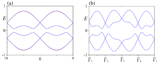
Figure S2: Superconducting boundary bands. (a) The parameters of the 2D BdG Hamiltonian are $\epsilon_{1,2}=0$, $m_{0}=0$, $m_{1}=1$, $m_{2}=2$, $\lambda_{1}=0.5$, $\lambda_{2}=1.0$, $\mu=0.3$, $\Delta_{0}=0$ and $\Delta_{1}=0.2$. The lattice size along the direction with open boundary condition is $100$ lattice spacings. The numerical (blue curves) and analytical (red curves) results show excellent agreement. (b) The parameters of the 3D BdG Hamiltonian are $\epsilon_{1,2,3}=0$, $m_{0}=0$, $m_{1,2}=1$, $m_{3}=3$, $\lambda_{1,2}=0.5$, $\lambda_{3}=1.5$, $\mu=0.3$, $\Delta_{0}=0.1$ and $\Delta_{1}=0.15$. The lattice size along the direction with open boundary condition is $100$ lattice spacings. The numerical (blue curves) and analytical (red curves) results show perfect agreement.

References

- Hasan and Kane (2010) M. Z. Hasan and C. L. Kane, “Colloquium : Topological insulators,” Rev. Mod. Phys. 82, 3045–3067 (2010).
- Qi and Zhang (2011) Xiao-Liang Qi and Shou-Cheng Zhang, “Topological insulators and superconductors,” Rev. Mod. Phys. 83, 1057–1110 (2011).
- Kane and Mele (2005) C. L. Kane and E. J. Mele, “ topological order and the quantum spin hall effect,” Phys. Rev. Lett. 95, 146802 (2005).
- Fu et al. (2007) Liang Fu, C. L. Kane, and E. J. Mele, “Topological insulators in three dimensions,” Phys. Rev. Lett. 98, 106803 (2007).
- Moore and Balents (2007) J. E. Moore and L. Balents, “Topological invariants of time-reversal-invariant band structures,” Phys. Rev. B 75, 121306 (2007).
- Roy (2009) Rahul Roy, “Topological phases and the quantum spin hall effect in three dimensions,” Phys. Rev. B 79, 195322 (2009).
- Fu and Kane (2007) Liang Fu and C. L. Kane, “Topological insulators with inversion symmetry,” PRB 76, 045302 (2007).
- König et al. (2007) Markus König, Steffen Wiedmann, Christoph Brüne, Andreas Roth, Hartmut Buhmann, Laurens W. Molenkamp, Xiao-Liang Qi, and Shou-Cheng Zhang, “Quantum spin hall insulator state in hgte quantum wells,” Science 318, 766–770 (2007), https://science.sciencemag.org/content/318/5851/766.full.pdf .
- Knez et al. (2011) Ivan Knez, Rui-Rui Du, and Gerard Sullivan, “Evidence for helical edge modes in inverted quantum wells,” Phys. Rev. Lett. 107, 136603 (2011).
- Wu et al. (2018) Sanfeng Wu, Valla Fatemi, Quinn D. Gibson, Kenji Watanabe, Takashi Taniguchi, Robert J. Cava, and Pablo Jarillo-Herrero, “Observation of the quantum spin hall effect up to 100 kelvin in a monolayer crystal,” Science 359, 76–79 (2018).
- Zhang et al. (2009) Haijun Zhang, Chao-Xing Liu, Xiao-Liang Qi, Xi Dai, Zhong Fang, and Shou-Cheng Zhang, “Topological insulators in bi2se3, bi2te3 and sb2te3 with a single dirac cone on the surface,” Nature Physics 5, 438–442 (2009).
- Chen et al. (2009) Y. L. Chen, J. G. Analytis, J.-H. Chu, Z. K. Liu, S.-K. Mo, X. L. Qi, H. J. Zhang, D. H. Lu, X. Dai, Z. Fang, S. C. Zhang, I. R. Fisher, Z. Hussain, and Z.-X. Shen, “Experimental realization of a three-dimensional topological insulator, bi2te3,” Science 325, 178–181 (2009), https://science.sciencemag.org/content/325/5937/178.full.pdf .
- Xia et al. (2009) Y. Xia, D. Qian, D. Hsieh, L. Wray, A. Pal, H. Lin, A. Bansil, D. Grauer, Y. S. Hor, R. J. Cava, and M. Z. Hasan, “Observation of a large-gap topological-insulator class with a single dirac cone on the surface,” Nature Physics 5, 398–402 (2009).
- Hsieh et al. (2009a) D. Hsieh, Y. Xia, D. Qian, L. Wray, F. Meier, J. H. Dil, J. Osterwalder, L. Patthey, A. V. Fedorov, H. Lin, A. Bansil, D. Grauer, Y. S. Hor, R. J. Cava, and M. Z. Hasan, “Observation of time-reversal-protected single-dirac-cone topological-insulator states in and ,” Phys. Rev. Lett. 103, 146401 (2009a).
- Liu et al. (2016) Cheng-Cheng Liu, Jin-Jian Zhou, Yugui Yao, and Fan Zhang, “Weak topological insulators and composite weyl semimetals: (, i),” Phys. Rev. Lett. 116, 066801 (2016).
- Noguchi et al. (2019) Ryo Noguchi, T. Takahashi, K. Kuroda, M. Ochi, T. Shirasawa, M. Sakano, C. Bareille, M. Nakayama, M. D. Watson, K. Yaji, A. Harasawa, H. Iwasawa, P. Dudin, T. K. Kim, M. Hoesch, V. Kandyba, A. Giampietri, A. Barinov, S. Shin, R. Arita, T. Sasagawa, and Takeshi Kondo, “A weak topological insulator state in quasi-one-dimensional bismuth iodide,” Nature 566, 518–522 (2019).
- Hsieh et al. (2009b) D. Hsieh, Y. Xia, D. Qian, L. Wray, J. H. Dil, F. Meier, J. Osterwalder, L. Patthey, J. G. Checkelsky, N. P. Ong, A. V. Fedorov, H. Lin, A. Bansil, D. Grauer, Y. S. Hor, R. J. Cava, and M. Z. Hasan, “A tunable topological insulator in the spin helical dirac transport regime,” Nature 460, 1101–1105 (2009b).
- Fu and Kane (2008) Liang Fu and C. L. Kane, “Superconducting proximity effect and majorana fermions at the surface of a topological insulator,” Phys. Rev. Lett. 100, 096407 (2008).
- Hosur et al. (2011) Pavan Hosur, Pouyan Ghaemi, Roger S. K. Mong, and Ashvin Vishwanath, “Majorana modes at the ends of superconductor vortices in doped topological insulators,” Phys. Rev. Lett. 107, 097001 (2011).
- Qin et al. (2019) Shengshan Qin, Lunhui Hu, Xianxin Wu, Xia Dai, Chen Fang, Fu-Chun Zhang, and Jiangping Hu, “Topological vortex phase transitions in iron-based superconductors,” Science Bulletin 64, 1207 – 1214 (2019).
- Yan et al. (2020) Zhongbo Yan, Zhigang Wu, and Wen Huang, “Vortex end majorana zero modes in superconducting dirac and weyl semimetals,” Phys. Rev. Lett. 124, 257001 (2020).
- Yan et al. (2018) Zhongbo Yan, Fei Song, and Zhong Wang, “Majorana corner modes in a high-temperature platform,” Phys. Rev. Lett. 121, 096803 (2018).
- Wang et al. (2018a) Qiyue Wang, Cheng-Cheng Liu, Yuan-Ming Lu, and Fan Zhang, “High-temperature majorana corner states,” Phys. Rev. Lett. 121, 186801 (2018a).
- Zhang et al. (2019a) Rui-Xing Zhang, William S. Cole, and S. Das Sarma, “Helical hinge majorana modes in iron-based superconductors,” Phys. Rev. Lett. 122, 187001 (2019a).
- Gray et al. (2019) Mason J. Gray, Josef Freudenstein, Shu Yang F. Zhao, Ryan O’Connor, Samuel Jenkins, Narendra Kumar, Marcel Hoek, Abigail Kopec, Soonsang Huh, Takashi Taniguchi, Kenji Watanabe, Ruidan Zhong, Changyoung Kim, G. D. Gu, and K. S. Burch, “Evidence for helical hinge zero modes in an fe-based superconductor,” Nano Letters 19, 4890–4896 (2019).
- Hsu et al. (2020) Yi-Ting Hsu, William S. Cole, Rui-Xing Zhang, and Jay D. Sau, “Inversion-protected higher-order topological superconductivity in monolayer ,” Phys. Rev. Lett. 125, 097001 (2020).
- Vu et al. (2020) DinhDuy Vu, Rui-Xing Zhang, and Sankar Das Sarma, “Time-reversal-invariant -symmetric higher-order topological superconductors,” (2020), arXiv:2005.03679 [cond-mat.supr-con] .
- Wu et al. (2020a) Yu-Biao Wu, Guang-Can Guo, Zhen Zheng, and Xu-Bo Zou, “Boundary-obstructed topological superfluids in staggered spin-orbit coupled fermi gases,” (2020a), arXiv:2007.15886 [cond-mat.quant-gas] .
- Yan (2019a) Zhongbo Yan, “Higher-order topological odd-parity superconductors,” Phys. Rev. Lett. 123, 177001 (2019a).
- Ahn and Yang (2020) Junyeong Ahn and Bohm-Jung Yang, “Higher-order topological superconductivity of spin-polarized fermions,” Phys. Rev. Research 2, 012060 (2020).
- Langbehn et al. (2017) Josias Langbehn, Yang Peng, Luka Trifunovic, Felix von Oppen, and Piet W. Brouwer, “Reflection-symmetric second-order topological insulators and superconductors,” Phys. Rev. Lett. 119, 246401 (2017).
- Shapourian et al. (2018) Hassan Shapourian, Yuxuan Wang, and Shinsei Ryu, “Topological crystalline superconductivity and second-order topological superconductivity in nodal-loop materials,” Phys. Rev. B 97, 094508 (2018).
- Khalaf (2018) Eslam Khalaf, “Higher-order topological insulators and superconductors protected by inversion symmetry,” Phys. Rev. B 97, 205136 (2018).
- Geier et al. (2018) Max Geier, Luka Trifunovic, Max Hoskam, and Piet W. Brouwer, “Second-order topological insulators and superconductors with an order-two crystalline symmetry,” Phys. Rev. B 97, 205135 (2018).
- Zhu (2018) Xiaoyu Zhu, “Tunable majorana corner states in a two-dimensional second-order topological superconductor induced by magnetic fields,” Phys. Rev. B 97, 205134 (2018).
- Wang et al. (2018b) Yuxuan Wang, Mao Lin, and Taylor L. Hughes, “Weak-pairing higher order topological superconductors,” Phys. Rev. B 98, 165144 (2018b).
- Hsu et al. (2018) Chen-Hsuan Hsu, Peter Stano, Jelena Klinovaja, and Daniel Loss, “Majorana kramers pairs in higher-order topological insulators,” Phys. Rev. Lett. 121, 196801 (2018).
- Liu et al. (2018a) Tao Liu, James Jun He, and Franco Nori, “Majorana corner states in a two-dimensional magnetic topological insulator on a high-temperature superconductor,” Phys. Rev. B 98, 245413 (2018a).
- Wu et al. (2019) Zhigang Wu, Zhongbo Yan, and Wen Huang, “Higher-order topological superconductivity: Possible realization in fermi gases and ,” Phys. Rev. B 99, 020508 (2019).
- Volpez et al. (2019) Yanick Volpez, Daniel Loss, and Jelena Klinovaja, “Second-order topological superconductivity in -junction rashba layers,” Phys. Rev. Lett. 122, 126402 (2019).
- Zhang et al. (2019b) Rui-Xing Zhang, William S. Cole, Xianxin Wu, and S. Das Sarma, “Higher-order topology and nodal topological superconductivity in fe(se,te) heterostructures,” Phys. Rev. Lett. 123, 167001 (2019b).
- Wu et al. (2019) Xianxin Wu, Xin Liu, Ronny Thomale, and Chao-Xing Liu, “High- Superconductor Fe(Se,Te) Monolayer: an Intrinsic, Scalable and Electrically-tunable Majorana Platform,” arXiv e-prints , arXiv:1905.10648 (2019), arXiv:1905.10648 [cond-mat.supr-con] .
- Zeng et al. (2019) Chuanchang Zeng, T. D. Stanescu, Chuanwei Zhang, V. W. Scarola, and Sumanta Tewari, “Majorana corner modes with solitons in an attractive hubbard-hofstadter model of cold atom optical lattices,” Phys. Rev. Lett. 123, 060402 (2019).
- Bultinck et al. (2019) Nick Bultinck, B. Andrei Bernevig, and Michael P. Zaletel, “Three-dimensional superconductors with hybrid higher-order topology,” Phys. Rev. B 99, 125149 (2019).
- Ghorashi et al. (2019) Sayed Ali Akbar Ghorashi, Xiang Hu, Taylor L. Hughes, and Enrico Rossi, “Second-order dirac superconductors and magnetic field induced majorana hinge modes,” Phys. Rev. B 100, 020509 (2019).
- Peng and Xu (2019) Yang Peng and Yong Xu, “Proximity-induced majorana hinge modes in antiferromagnetic topological insulators,” Phys. Rev. B 99, 195431 (2019).
- Zhu (2019) Xiaoyu Zhu, “Second-order topological superconductors with mixed pairing,” Phys. Rev. Lett. 122, 236401 (2019).
- Laubscher et al. (2019) Katharina Laubscher, Daniel Loss, and Jelena Klinovaja, “Fractional topological superconductivity and parafermion corner states,” Phys. Rev. Research 1, 032017 (2019).
- Pan et al. (2019) Xiao-Hong Pan, Kai-Jie Yang, Li Chen, Gang Xu, Chao-Xing Liu, and Xin Liu, “Lattice-symmetry-assisted second-order topological superconductors and majorana patterns,” Phys. Rev. Lett. 123, 156801 (2019).
- Yan (2019b) Zhongbo Yan, “Majorana corner and hinge modes in second-order topological insulator/superconductor heterostructures,” Phys. Rev. B 100, 205406 (2019b).
- Franca et al. (2019) S. Franca, D. V. Efremov, and I. C. Fulga, “Phase-tunable second-order topological superconductor,” Phys. Rev. B 100, 075415 (2019).
- Kheirkhah et al. (2020a) Majid Kheirkhah, Yuki Nagai, Chun Chen, and Frank Marsiglio, “Majorana corner flat bands in two-dimensional second-order topological superconductors,” Phys. Rev. B 101, 104502 (2020a).
- Zhang and Trauzettel (2020) Song-Bo Zhang and Björn Trauzettel, “Detection of second-order topological superconductors by josephson junctions,” Phys. Rev. Research 2, 012018 (2020).
- Roy (2020) Bitan Roy, “Higher-order topological superconductors in -, -odd quadrupolar dirac materials,” Phys. Rev. B 101, 220506 (2020).
- Wu et al. (2020b) Ya-Jie Wu, Junpeng Hou, Yun-Mei Li, Xi-Wang Luo, Xiaoyan Shi, and Chuanwei Zhang, “In-plane zeeman-field-induced majorana corner and hinge modes in an -wave superconductor heterostructure,” Phys. Rev. Lett. 124, 227001 (2020b).
- Kheirkhah et al. (2020b) Majid Kheirkhah, Zhongbo Yan, Yuki Nagai, and Frank Marsiglio, “First- and second-order topological superconductivity and temperature-driven topological phase transitions in the extended hubbard model with spin-orbit coupling,” Phys. Rev. Lett. 125, 017001 (2020b).
- Wu et al. (2020c) Xianxin Wu, Wladimir A. Benalcazar, Yinxiang Li, Ronny Thomale, Chao-Xing Liu, and Jiangping Hu, “Boundary-obstructed topological high-tc superconductivity in iron pnictides,” (2020c), arXiv:2003.12204 [cond-mat.supr-con] .
- Tiwari et al. (2020) Apoorv Tiwari, Ammar Jahin, and Yuxuan Wang, “Chiral dirac superconductors: Second-order and boundary-obstructed topology,” (2020), arXiv:2005.12291 [cond-mat.mes-hall] .
- Ono et al. (2020a) Seishiro Ono, Hoi Chun Po, and Haruki Watanabe, “Refined symmetry indicators for topological superconductors in all space groups,” Science Advances 6 (2020a), 10.1126/sciadv.aaz8367, https://advances.sciencemag.org/content/6/18/eaaz8367.full.pdf .
- Ono et al. (2020b) Seishiro Ono, Hoi Chun Po, and Ken Shiozaki, “-enriched symmetry indicators for topological superconductors in the 1651 magnetic space groups,” (2020b), arXiv:2008.05499 [cond-mat.supr-con] .
- Wang et al. (2015) Zhijun Wang, P. Zhang, Gang Xu, L. K. Zeng, H. Miao, Xiaoyan Xu, T. Qian, Hongming Weng, P. Richard, A. V. Fedorov, H. Ding, Xi Dai, and Zhong Fang, “Topological nature of the superconductor,” Phys. Rev. B 92, 115119 (2015).
- Wu et al. (2016) Xianxin Wu, Shengshan Qin, Yi Liang, Heng Fan, and Jiangping Hu, “Topological characters in thin films,” Phys. Rev. B 93, 115129 (2016).
- Xu et al. (2016) Gang Xu, Biao Lian, Peizhe Tang, Xiao-Liang Qi, and Shou-Cheng Zhang, “Topological superconductivity on the surface of fe-based superconductors,” Phys. Rev. Lett. 117, 047001 (2016).
- Zhang et al. (2018) Peng Zhang, Koichiro Yaji, Takahiro Hashimoto, Yuichi Ota, Takeshi Kondo, Kozo Okazaki, Zhijun Wang, Jinsheng Wen, GD Gu, Hong Ding, et al., “Observation of topological superconductivity on the surface of an iron-based superconductor,” Science 360, 182–186 (2018).
- Wang et al. (2018c) Dongfei Wang, Lingyuan Kong, Peng Fan, Hui Chen, Shiyu Zhu, Wenyao Liu, Lu Cao, Yujie Sun, Shixuan Du, John Schneeloch, et al., “Evidence for majorana bound states in an iron-based superconductor,” Science 362, 333–335 (2018c).
- Kong et al. (2019) Lingyuan Kong, Shiyu Zhu, Michał Papaj, Hui Chen, Lu Cao, Hiroki Isobe, Yuqing Xing, Wenyao Liu, Dongfei Wang, Peng Fan, et al., “Half-integer level shift of vortex bound states in an iron-based superconductor,” Nature Physics , 1–7 (2019).
- Machida et al. (2019) T Machida, Y Sun, S Pyon, S Takeda, Y Kohsaka, T Hanaguri, T Sasagawa, and T Tamegai, “Zero-energy vortex bound state in the superconducting topological surface state of fe (se, te),” Nature materials , 1 (2019).
- Liu et al. (2018b) Qin Liu, Chen Chen, Tong Zhang, Rui Peng, Ya-Jun Yan, Chen-Hao-Ping Wen, Xia Lou, Yu-Long Huang, Jin-Peng Tian, Xiao-Li Dong, Guang-Wei Wang, Wei-Cheng Bao, Qiang-Hua Wang, Zhi-Ping Yin, Zhong-Xian Zhao, and Dong-Lai Feng, “Robust and clean majorana zero mode in the vortex core of high-temperature superconductor ,” Phys. Rev. X 8, 041056 (2018b).
- Chen et al. (2019) C Chen, Q Liu, TZ Zhang, D Li, PP Shen, XL Dong, Z-X Zhao, T Zhang, and DL Feng, “Quantized conductance of majorana zero mode in the vortex of the topological superconductor (li0. 84fe0. 16) ohfese,” Chinese Physics Letters 36, 057403 (2019).
- Zhu et al. (2020) Shiyu Zhu, Lingyuan Kong, Lu Cao, Hui Chen, Michał Papaj, Shixuan Du, Yuqing Xing, Wenyao Liu, Dongfei Wang, Chengmin Shen, Fazhi Yang, John Schneeloch, Ruidan Zhong, Genda Gu, Liang Fu, Yu-Yang Zhang, Hong Ding, and Hong-Jun Gao, “Nearly quantized conductance plateau of vortex zero mode in an iron-based superconductor,” Science 367, 189–192 (2020).
- Mazin et al. (2008) I. I. Mazin, D. J. Singh, M. D. Johannes, and M. H. Du, “Unconventional superconductivity with a sign reversal in the order parameter of ,” Phys. Rev. Lett. 101, 057003 (2008).
- Wang and Lee (2011) Fa Wang and Dung-Hai Lee, “The electron-pairing mechanism of iron-based superconductors,” Science 332, 200–204 (2011).
- Schnyder et al. (2008) Andreas P. Schnyder, Shinsei Ryu, Akira Furusaki, and Andreas W. W. Ludwig, “Classification of topological insulators and superconductors in three spatial dimensions,” Phys. Rev. B 78, 195125 (2008).
- Kitaev (2009) Alexei Kitaev, “Periodic table for topological insulators and superconductors,” in AIP Conference Proceedings, Vol. 1134 (AIP, 2009) pp. 22–30.
- Haim and Oreg (2019) Arbel Haim and Yuval Oreg, “Time-reversal-invariant topological superconductivity in one and two dimensions,” Physics Reports 825, 1 – 48 (2019), time-reversal-invariant topological superconductivity in one and two dimensions.
- Qi et al. (2010) Xiao-Liang Qi, Taylor L. Hughes, and Shou-Cheng Zhang, “Topological invariants for the fermi surface of a time-reversal-invariant superconductor,” Phys. Rev. B 81, 134508 (2010).
- (77) The supplemental material contains the derivation of boundary Hamiltonians.
- Wong and Law (2012) Chris L. M. Wong and K. T. Law, “Majorana kramers doublets in -wave superconductors with rashba spin-orbit coupling,” Phys. Rev. B 86, 184516 (2012).
- Zhang et al. (2013) Fan Zhang, C. L. Kane, and E. J. Mele, “Time-reversal-invariant topological superconductivity and majorana kramers pairs,” Phys. Rev. Lett. 111, 056402 (2013).
- Keselman et al. (2013) Anna Keselman, Liang Fu, Ady Stern, and Erez Berg, “Inducing time-reversal-invariant topological superconductivity and fermion parity pumping in quantum wires,” Phys. Rev. Lett. 111, 116402 (2013).
- Haim et al. (2014) Arbel Haim, Anna Keselman, Erez Berg, and Yuval Oreg, “Time-reversal-invariant topological superconductivity induced by repulsive interactions in quantum wires,” Phys. Rev. B 89, 220504 (2014).
- Gaidamauskas et al. (2014) Erikas Gaidamauskas, Jens Paaske, and Karsten Flensberg, “Majorana bound states in two-channel time-reversal-symmetric nanowire systems,” Phys. Rev. Lett. 112, 126402 (2014).
- Schrade et al. (2015) Constantin Schrade, A. A. Zyuzin, Jelena Klinovaja, and Daniel Loss, “Proximity-induced josephson junctions in topological insulators and kramers pairs of majorana fermions,” Phys. Rev. Lett. 115, 237001 (2015).
- Deng et al. (2012) Shusa Deng, Lorenza Viola, and Gerardo Ortiz, “Majorana modes in time-reversal invariant -wave topological superconductors,” Phys. Rev. Lett. 108, 036803 (2012).
- Kheirkhah et al. (2020c) Majid Kheirkhah, Zhongbo Yan, and Frank Marsiglio, “Vortex line topology in iron-based superconductors with and without second-order topology,” (2020c), arXiv:2007.10326 [cond-mat.supr-con] .
Supplemental Material “Boundary Topological Superconductors”
Bo-Xuan Li1, Zhongbo Yan1,∗
1School of Physics, Sun Yat-sen University, Guangzhou, 510275, China