Topological and nematic superconductivity mediated by ferro-SU(4) fluctuations in twisted bilayer graphene

Abstract

We propose an SU(4) spin-valley-fermion model to investigate the superconducting instabilities of twisted bilayer graphene (TBG). In this approach, bosonic fluctuations associated with an emergent SU(4) symmetry, corresponding to combined rotations in valley and spin spaces, couple to the low-energy fermions that comprise the flat bands. These fluctuations are peaked at zero wave-vector, reflecting the “ferromagnetic-like” SU(4) ground state recently found in strong-coupling solutions of microscopic models for TBG. Focusing on electronic states related to symmetry-imposed points of the Fermi surface, dubbed here “valley hot-spots” and “van Hove hot-spots”, we find that the coupling to the itinerant electrons partially lifts the huge degeneracy of the ferro-SU(4) ground state manifold, favoring inter-valley order, spin-valley coupled order, ferromagnetic order, spin-current order, and valley-polarized order, depending on details of the band structure. These fluctuations, in turn, promote attractive pairing interactions in a variety of closely competing channels, including a nodeless $f$-wave state, a nodal $i$-wave state, and topological $d+id$ and $p+ip$ states with unusual Chern numbers $2$ and $4$, respectively. Nematic superconductivity, although not realized as a primary instability of the system, appears as a consequence of the near-degeneracy of superconducting order parameters that transform as one-dimensional and two-dimensional irreducible representations of the point group $D_{6}$.

I Introduction

The recent discovery of correlated insulating and superconducting phases in twisted bilayer graphene (TBG) near the magic angle has brought this system in the limelight of condensed matter physics Pablo1 ; Pablo2 ; David ; Young ; Cory1 ; Cory2 ; Dmitry1 ; Ashoori ; Dmitry2 ; Yazdani ; Eva ; Yazdani2 ; Shahal ; Young2 . Similar phenomena have also been identified in other moiré systems, such as twisted double bilayer graphene Pablo3 ; Guanyu ; Kim , twisted trilayer systems Feng ; Feng2 ; Feng3 ; KeWang19 , and transition metal dichalcogenide moiré heterostructures Shan20 , illustrating that the observed correlated electronic phases are rather universal in moiré systems. In addition to the insulating and superconducting phases, electronic nematic order Cory2 ; Perge ; Eva ; Cao20 and ferromagnetism David ; Young ; Dmitry1 ; YoungFM20 have also been observed in TBG. Since many of these correlated phases are also observed in unconventional superconductors, it is interesting to compare the role of electronic correlations in these different systems Leon1 ; LiangPRX1 ; KangVafekPRX ; Senthil1 ; FanYang ; Louk ; LiangPRX2 ; GuineaPNAS ; Kivelson ; Fernandes1 ; Guo ; Kuroki ; Qianghua ; Stauber ; KangVafekPRL ; Bruno ; Senthil2 ; Ashvin1 ; Cenke ; MacDonald ; Sachdev18 ; Zalatel1 ; Zalatel2 ; Guinea20 ; Senthil3Ferro ; Sau ; Ashvin2 ; Zalatel3 ; Dai2 ; YiZhang ; Kang3 ; Chichinadze20 ; ZYMeng20 ; You ; Rossi ; Bernevig20 ; Torma ; Ashvin20 ; DasSarma ; Zaletel2005 ; Debanjan20 ; Balents20 ; SachdevPNAS ; MacDonald20 ; Nandkishore219 ; Adam . At first sight, this seems to be a formidable task, because the tiny twist angles of TBG lead to a huge unit cell containing more than $10^{4}$ atoms. However, it is widely understood now that the correlated phases in TBG arise from the narrow bands around the charge neutrality point (CNP), which are separated from the remote bands by a band gap of tens of meV Bistritzer11 ; Mele11 . Such an observation suggests that low-energy models focusing on the four narrow bands can shed important light on the properties of TBG.

Due to the small bandwidth of these narrow bands, the kinetic energy is comparable to the Coulomb interaction, pointing to the crucial role played by electronic correlations in shaping the phase diagram of TBG. Because the the Coulomb repulsion, estimated as $e^{2}/(\epsilon_{hBN}L_{m})\approx 24$meV, is comparable with the calculated bandwidth Bistritzer11 , there have been parallel efforts on analyzing the system theoretically from both a strong-coupling Leon1 ; LiangPRX1 ; Senthil1 ; Louk ; KangVafekPRL ; Kivelson ; Fernandes1 ; Zalatel3 ; Kang3 ; Ashvin20 and a weak-coupling perspective MacDonald ; LiangPRX2 ; Nandkishore19 ; Bitan2019 ; Dai2 ; Guinea20 ; YiZhang ; DasSarma20 ; Chichinadze20 ; LinNandkishore20 . On the one hand, correlated insulating phases are experimentally observed at commensurate fillings of the moiré superlattice Pablo1 ; Cory1 ; Dmitry1 ; Shahal ; Yazdani2 , highlighting the importance of strong correlations. On the other hand, van Hove singularities that occur at specific concentrations have been proposed to host a variety of weak-coupling instabilities LiangPRX2 ; DasSarma20 ; Chichinadze20 , some of which may have been observed experimentally Cao20 . In either approach, the correlated insulating state often breaks a symmetry of the system. While it remains unsettled which – if any – symmetries are broken in the correlated states of TBG, the fact that superconductivity appears once the correlated state is suppressed suggests that fluctuations associated with the broken symmetry of the correlated state may be responsible for the formation of the Cooper pairs. Such a scenario parallels others widely employed to model unconventional superconductors, such as pairing in the vicinity of an antiferromagnetic state Scalapino12 . Of course, it is possible that the superconductivity in TBG is a standard electron-phonon pairing state, as proposed elsewhere Wu18 ; Bernevig19 ; Fabrizio19 . Recent experiments also observed superconductivity in devices where the strength of the correlations is suppressed, e.g. by decreasing the distance between the metallic gates, by moving the system away from the magic twist angle Dmitry2 ; Young2 ; Harpreet20 . Whether this is an indication that pairing does not require correlations or that fluctuations associated with the correlated state persist even after the latter is suppressed remains under debate.

In this paper, we investigate the scenario in which superconductivity in TBG arises from the fluctuations associated with the suppressed correlated ordered state. We illustrate this scenario for superconductivity in the schematic phase diagram shown in Fig. 1. Instead of choosing between a strong-coupling or a weak-coupling approach, we attempt to bridge them by adopting a more phenomenological approach, similar in spirit to the spin-fermion models widely employed to study magnetically-mediated superconductivity in cuprates and heavy fermions Abanov03 ; Roussev01 ; Metlitski10 ; Wang13 ; Wang17 . The traditional spin-fermion model is rooted in a separation of energy scales: high-energy states give rise to an antiferromagnetic (or ferromagnetic) SU(2) order parameter, while low-energy states interact with each other via the exchange of fluctuations associated with this order parameter. In this type of model, antiferromagnetic (ferromagnetic) fluctuations are known to promote unconventional $d$-wave ($p$-wave) pairing. It has been recently generalized to consider more generic bosonic excitations, such as nematic Lederer15 ; Kang16 ; Klein19 and ferroelectric fluctuations KoziiFu ; WangCho ; Gastiasoro20 , which favor multiple pairing states simultaneously.

Figure 1: Schematic phase diagram of superconductivity mediated by fluctuations associated with a correlated state that displays “ferromagnetic-like” SU(4) order. As we show in this paper, the types of ferro-SU(4) order favored by the coupling to itinerant fermions are inter-valley order, spin-valley coupled order, ferromagnetic order, spin-current order, and valley-polarized order. As shown in Table 1, these fluctuations promote a rich landscape of pairing states, such as a nodeless $f$-wave state, a nodal $i$-wave state, and topological $d+id$ and $p+ip$ states with unusual Chern numbers $2$ and $4$, respectively.

In TBG, the existence of well-separated energy scales is not as obvious as in other quantum materials. Yet, given the difficulties in building microscopic Hamiltonians for TBG and other moiré systems, and the powerful insights that boson-fermion types of models have provided to other quantum materials, it is interesting to build such a model for TBG and investigate its predictions for the possible superconducting states. In this regard, one of the most striking differences between TBG and other unconventional superconductors is that, in the former, the fermions are labeled by both spin and valley degrees of freedom. Because of the negligibly small spin-orbit coupling of graphene, SU(2) spin-rotational invariance is preserved. Moreover, TBG has an approximate U(1) valley symmetry, related to the suppressed coupling between the two opposite valleys of the graphene sheets for small twist angles Senthil1 . Consequently, a sensible starting point is a low-energy model with (approximate) SU(2)$\otimes$SU(2)$\otimes$U(1) symmetry, where the two SU(2) groups correspond to independent spin rotations on the two valleys. Because this is a subgroup of SU(4), it is often convenient to label the possible ordered states in terms of a maximally symmetric bosonic SU(4) order parameter $\hat{\Phi}$, related to rotations in the combined spin and valley spaces, and thus characterized by $15$ independent components Leon1 ; Fernandes1 ; Classen19 ; Natori19 ; KangVafekPRL . Interestingly, several low-energy microscopic Hamiltonians have been proposed for TBG whose interacting parts display an emergent SU(4) symmetry at the energy scale of the flat bands, which is generally broken by the kinetic part. Strong coupling analyses have shown that the ground state in this SU(4) manifold is “ferromagnetic-like,” i.e. it is described by an order parameter $\hat{\Phi}$ that condenses at zero-momentum, without breaking translational symmetry KangVafekPRL ; Bruno . Recent Quantum Monte Carlo simulations also found ferro-SU(4) ground states ZYMeng20 . Experimentally, this is consistent with the observation of ferromagnetism in TBG at certain fillings David ; Young ; YoungFM20 . Importantly, the emergence at strong coupling of a ferromagnetic-like state, as opposed to the more usual antiferromagnetic-like state, is closely tied to the fragile topology of the flat bands KangVafekPRL ; Zalatel1 ; Zalatel2 ; Senthil3Ferro ; Kang3 . Whether such a ferro-SU(4) state can be obtained directly within a weak-coupling low-energy theory remains to be seen. Interestingly, the mean-field analysis of a related model that has SU(2) spin-rotational symmetry and U(1) orbital symmetry found a “ferromagnetic-like” ground state, which can be either orbital nematic or orbital ferromagnetic Kivelson . This orbitally ordered state forms a dome in the temperature-doping phase diagram, giving rise to two smaller spin-singlet orbital-triplet superconducting domes at its edges, similarly to our sketch in Fig. 1. As we will show below, our analysis, which includes fluctuations of the ordered state, also find regimes of spin-singlet valley-triplet superconductivity.

The goal of our phenomenological model is to provide a useful platform to analyze the effects of strong coupling physics on the itinerant fermions. Denoting the low-energy fermionic creation operators by $\psi_{\alpha a}^{\dagger}$, with $\alpha=\pm 1\equiv\pm K$ referring to the valley degrees of freedom and $a=\uparrow,\downarrow$, to the spin degrees of freedom, the coupling between the boson $\hat{\Phi}$ and the low-energy fermions is given by:

$$H_{\mathrm{int}}=g\phi_{\mu\nu}\,\psi_{\alpha a}^{\dagger}\tau_{\alpha\beta}^{\mu}\sigma_{ab}^{\nu}\psi_{\beta b},$$ (1)

where $g$ is a coupling constant and the Pauli matrices $\boldsymbol{\tau}$ and $\boldsymbol{\sigma}$ act on valley space and on spin space, respectively (summation over repeated indices is left implicit). Here, $\phi_{\mu\nu}$ are the 15 components of $\hat{\Phi}$ with $\mu,\,\nu=0,...,\,3$ subject to the constraint that $\mu=\nu=0$ is excluded; this last condition arises because $\phi_{00}$ is just a constant that can be absorbed in the definition of the chemical potential. We dub this phenomenological low-energy model the SU(4) spin-valley-fermion model.

Table 1: A summary of the superconducting instabilities mediated by the exchange of ferro-SU(4) fluctuations in different channels (first and second columns). The pairing nomenclature in the third column ($s,\,p,\,d$, etc) is explained in the main text in terms of the irreducible representations of the $D_{6}$ group. The Chern number of each pairing state in the third column is respectively shown in the fourth column. The last column shows what combination of pairing states generate a subsidiary nematic order.

SU(4) channel	SU(4) ground state	Pairing	Chern number	Nematicity
$\phi_{v}$	inter-valley	valley-triplet: $A_{1}$ ($s$-wave), $E_{2}$ ($d\pm id$), $E_{1}$ ($p\pm ip$)	0, 4, 2	$s\pm d$
$\phi_{sv}$	spin-valley	spin-singlet & valley-singlet: $E_{2}$ ($d$$\pm id$), $A_{2}$ ($i$-wave)	2, N/A	$i\pm d$
$\phi_{s}$	ferromagnetic	spin-triplet: $B_{2}$ ($f$-wave), $E_{1}$ ($p\pm ip$)	0, 4	$p\pm f$
$\phi_{sc}$	spin-current	spin-singlet: $A_{1}$ ($s$-wave), $E_{2}$ ($d\pm id$)	0, 2	$s\pm d$
$\phi_{vp}$	valley-polarized	no Cooper instability	N/A	N/A

Here, we investigate the superconducting (SC) states — and their accompanying topological and lattice symmetry-breaking properties — that are mediated by the exchange of ferro-SU(4) fluctuations between low-energy fermions. In a single-band metal, it is well known that ferromagnetic SU(2) fluctuations cause repulsion in the conventional $s$-wave spin-singlet pairing channel and attraction in the $p$-wave spin-triplet channel Roussev01 . In our case, because of the multi-flavor nature of the fermions and of the much larger SU(4) manifold of the bosonic field, the model has a richer structure in terms of bosonic fluctuations and pairing channels Fernandes1 ; Scheurer20 ; Sachdev20 . In particular, because the dispersion of the low-energy fermions explicitly breaks the emergent SU(4) symmetry, we find that the boson-fermion coupling of Eq. (1) lifts the SU(4) degeneracy and restricts the soft fluctuations to a few distinct channels, namely: the ferromagnetic channel, characterized by $\phi_{s}\equiv\phi_{0i}$; the spin-current channel, given by $\phi_{sc}\equiv\phi_{3i}$; the inter-valley channel, described by $\phi_{v}\equiv\phi_{(1,2)0}$; the valley-polarization channel, described by $\phi_{vp}\equiv\phi_{30}$; and the spin-valley coupled channel, associated with $\phi_{sv}\equiv\phi_{(1,2)i}$. Despite the fact that the detailed band structure and the corresponding Fermi surface (FS) of TBG remain under debate, we argue that the selection of the strongest SU(4)-fluctuations channels, as well as of the corresponding leading pairing instabilities, depend only on robust features of the FS. In particular, when the FS of a given valley is close to a van Hove singularity LiangPRX2 ; FuNC ; Chichinadze19 , the coupling to the so-called van Hove hot-spots (see Fig. 2(b)) enhances the bosonic fluctuations in the intra-valley spin ferromagnetic channel ($\phi_{s}$), the spin current channel ($\phi_{sc}$), and the valley-polarized channel ($\phi_{vp}$). On the other hand, the coupling to states close to the intersections of the FSs formed by the two valleys (called valley hot-spots, see Fig. 2(a)) strongly enhances fluctuations in the inter-valley channel, which can be either in the density sector ($\phi_{v}$) or in the the spin sector ($\phi_{sv}$).

A comparative analysis of the strength of these different SU(4)-fluctuations channels requires microscopic details of the band structure beyond the scope of this work. Instead, we analyze the pairing states induced by each channel separately, discussing their implications to the phase diagram of TBG. A crucial point is that the pairing symmetry, as well as the topology of the induced SC order by each $\phi_{\mu\nu}$, can be obtained without detailed knowledge of the FS, by linearizing the low-energy fermionic dispersions around the van Hove and valley hot-spots. Due to the multi-flavor nature of the fermions and the ferro-like nature of the SU(4) fluctuations, which are peaked at zero momentum, we find that for all SU(4) channels considered, multiple pairing channels are simultaneously enhanced. Qualitative energetic arguments are then made to determine the leading pairing channels. Our main results are summarized in Table 1, which displays the leading pairing states favored by the different SU(4)-fluctuations channels discussed above. As indicated by their Chern numbers, several of these states are topologically non-trivial superconductors. Moreover, because multiple orthogonal pairing channels are simultaneously favored by a given sector of SU(4) fluctuations, this opens up the possibility of accidental degeneracy between different superconducting states. In the vicinity of such an accidental degeneracy, the sixfold rotational symmetry of the moiré lattice can be broken. The latter case gives rise to an accompanying electronic nematic order inside the superconducting state, as recently observed experimentally Cao20 .

The remainder of the paper is organized as follows. In Sec. II we present the SU(4) spin-valley-fermion model, and in Sec. III we discuss the lifting of the maximal SU(4) symmetry in the normal state. In Sec. IV we analyze the leading pairing channels induced by various SU(4) fluctuation channels and their symmetry-breaking and topological properties. In Sec. V we show that in all channels considered, the near-degenerate pairing channels can further induce an additional nematic order parameter. Conclusions are presented in Sec. VI.

II The SU(4) spin-valley-fermion model

We consider itinerant fermions coupled to soft SU(4) fluctuations peaked at zero momentum, i.e. “ferro-SU(4)” fluctuations. In each moiré unit cell, there are three relevant fermionic degree of freedom – moiré sublattice, spin, and valley — giving rise to four spin-degenerate nearly-flat bands. Here, “valley” refers to the valleys of the underlying graphene atomic lattice and not to the valleys of the moiré Brillouin zone. If the twist angle is small, electrons with different valley indices do not mix, and one can approximately treat valley as a good quantum number. Thus each low-energy fermion can be labeled by its valley and spin quantum numbers.

The action of the SU(4) spin-valley-fermion model is written as

$$\mathcal{S}=\int d\bm{k}d\omega\left[\Psi^{\dagger}(\omega,\bm{k})(-i\omega+\hat{\epsilon}(\bm{k}))\Psi(\omega,\bm{k})\right.$$

$$+\left.g\Psi^{\dagger}(\omega,\bm{k})\hat{\Phi}(\omega-\omega^{\prime},\bm{k}-\bm{k}^{\prime})\Psi(\omega^{\prime},\bm{k}^{\prime})\right]$$

$$+\frac{1}{2}\int d\bm{q}d\Omega\ (r+\alpha\Omega^{2}+\beta\bm{q}^{2})\operatorname{Tr}[\hat{\Phi}(\Omega,\bm{q})\hat{\Phi}(\Omega,\bm{q})],$$ (2)

where $g$ is a coupling constant, $\Psi$ is a four-component spinor that combines spin and valley degrees of freedom, and the bosonic order parameter $\hat{\Phi}$ is a four-by-four matrix that satisfies $\operatorname{Tr}(\hat{\Phi})=0$. Notice that we work in the band basis and have only kept the two bands (per spin) that give rise to Fermi surfaces LiangPRX1 ; KangVafekPRX . One can expand the field $\hat{\Phi}$ as a linear superposition of the 15 generators $\lambda_{i}$ of SU(4), $\hat{\Phi}(\Omega,\bm{q})=\sum_{i=1}^{15}\phi_{i}(\Omega,\bm{q})\lambda_{i}$. Without the kinetic energy term $\hat{\epsilon}(\bm{k})$, this model has an SU(4) symmetry, under which the 15 bosonic fields $\phi_{i}$ transform in the adjoint representation. Here, the quantity $(r+\alpha\Omega^{2}+\beta\bm{q}^{2})$ in the last term is the (bare) inverse propagator of the bosonic fluctuations. At the bare level, when $r$ becomes negative, the $\hat{\Phi}$ field condenses at zero-momentum and the system enters a ferro-SU(4) ordered state. Unlike the usual SU(2) spin-ferromagnetic states, the fermions can order in the spin, valley, and spin-valley coupling channels, and the ground state manifold has a much larger symmetry.

For our purposes, it is more convenient to reexpress the matrix field $\hat{\Phi}$ in terms of the tensor product of spin and valley Pauli matrices, $\tau^{\mu}\otimes\sigma^{\nu}$:

$$\hat{\Phi}(\Omega,\bm{q})={\sum_{\mu,\nu=0}^{3}}{}^{\prime}\,\phi_{\mu\nu}(\Omega,\bm{q})\tau^{\mu}\otimes\sigma^{\nu}$$ (3)

where the summation $\sum^{\prime}$ excludes the term $\mu=\nu=0$.

The SU(4) symmetry is broken explicitly by the free-fermion term of the action (2). In particular, the fermionic dispersion of the two valleys from the underlying atomic lattice (labeled by $K$ and $K^{\prime}=-K$) are distinct:

$$\hat{\epsilon}(\bm{k})=\left[\frac{\epsilon_{K}(\bm{k})+\epsilon_{K^{\prime}}(\bm{k})}{2}\tau^{0}+\frac{\epsilon_{K}(\bm{k})-\epsilon_{K^{\prime}}(\bm{k})}{2}\tau^{3}\right]\otimes\sigma^{0}$$ (4)

where $\epsilon_{K}(\bm{k})\neq\epsilon_{K^{\prime}}(\bm{k})$ and hereafter we will omit the $\otimes$ sign for compactness. Due to the approximate valley symmetry, the system transforms under the point group $D_{6}$. The fermionic dispersions associated with the $K$ and $K^{\prime}$ valleys are invariant under the three-fold rotation around the $z$-axis, $C_{3z}$, and the in-plane two-fold rotation $C_{2y}$. Additionally, the two valleys swap under the other in-plane two-fold rotation $C_{2x}$ and the two-fold rotation around the $z$-axis $C_{2z}$, as well as the $C_{6z}$ rotation. By these symmetry requirements, fermions in each valley give rise to a Fermi surface (FS) that has the same symmetry as a triangle, as illustrated in Fig. 2, and the two FSs are related by $C_{2z}$ (or, alternatively, $C_{2x}$ and $C_{6z}$). The exact shape of the FSs will strongly depend on the details of the microscopic hopping parameters, which remain unclear at present. However, much of our analysis does not rely on such details.

It is instructive to analyze the transformation properties under $D_{6}$ and time-reversal symmetries in the valley subspace. The elements in $D_{6}$ that act non-trivially in valley subspace are $C_{6}$, $C_{2z}$, and $C_{2x}$, all of which exchange the two valleys and are represented by $\tau^{1}$. As a result, the valley matrix $\tau^{1}$ transforms as $\tau^{1}\to C_{6}\tau^{1}C_{6}^{-1}\equiv\tau^{1}$, and thus belongs to the irreducible representation (irrep) $A_{1}$ of $D_{6}$. By the same token, $\tau^{2}$ and $\tau^{3}$ belong to irrep $B_{2}$. Moreover, time reversal $\mathcal{T}$ also swaps the two valleys, i.e., $\mathcal{T}=\tau^{1}K$, where $K$ is complex conjugation. Under time-reversal, $\tau^{1}$ and $\tau^{2}$ are even but $\tau^{3}$ is odd. We list the details of these transformation properties in Table 2. We note that in the Wannier orbital basis in which the ferro-SU(4) state is most intuitively derived, the point group symmetry is lowered to $D_{3}$, unless one includes additional orbitals that form high-energy bands. This is a result of the fragile topology of the flat bands that dictates that the $C_{2z}$ symmetry cannot be implemented locally in the Wannier basis Senthil1 ; KangVafekPRX . Since we work in the band basis, this issue is avoided.

Table 2: Transformation properties of the Pauli matrices in valley subspace under the symmetry operations $C_{2z}$ and time reversal $\mathcal{T}$.

valley matrix	irrep of $D_{6}$	$C_{2z}=\tau^{1}$	$\mathcal{T}=\tau^{1}K$
$\tau^{1}$	$A_{1}$	1	1
$\tau^{2}$	$B_{2}$	$-$1	1
$\tau^{3}$	$B_{2}$	$-$1	$-$1

As discussed in the Introduction, we take the existence of a ferro-SU(4) ground state as an input of our model, motivated by strong-coupling analyses, Quantum Monte Carlo simulations, and experimental results showing yet no evidence of translational symmetry breaking inside the insulating phases. In this sense, we assume a separation of energy scales, such that strong-coupling effects give rise to a largely degenerate ferro-SU(4) ground state. Upon suppression of the insulating ferro-SU(4) ground state, which can be achieved by doping or by increasing the separation between the metallic gates of TBG (which causes a suppression of the Coulomb repulsion Dmitry2 ), ferro-SU(4) fluctuations persist and then couple to the low-energy fermions. Our goal is then twofold: (i) to determine which SU(4) fluctuation channels, represented by $\phi_{\mu\nu}$, are enhanced by the coupling to the fermions, as the fermionic dispersion explicitly breaks the SU(4) symmetry; and (ii) to determine which pairing states are favored by those enhanced SU(4) fluctuations. These two problems are addressed in the upcoming Sections III and IV, respectively. The system is strongly coupled when the SU(4) fluctuations are soft, i.e., when the mass term $r$ is renormalized to zero, potentially leading to non-Fermi liquid and strange metal behaviors. However, in this work we focus on the symmetries of the ferro-SU(4) fluctuations and the types of pairing symmetries, leaving a detailed analysis of the dynamics of the coupled boson-fermion system to future work.

III Lifting of SU(4) degeneracy

As discussed above, the kinetic part of the Hamiltonian, Eq. (4), lifts the emergent SU(4) degeneracy of the interacting part. Despite the lack of complete knowledge of $\epsilon_{K}(\bm{k})$ and $\epsilon_{K^{\prime}}(\bm{k})$, their effect on selecting particular SU(4)-fluctuations channels can be deduced from the symmetry-imposed features of the Fermi surface and from the coupling in Eq. (1).

First, due to the approximate absence of inter-valley coupling, the two sets of FSs formed by valleys $K$ and $K^{\prime}$ intersect at points that are invariant under the rotations $C_{2x}$ and $C_{2z}$. Following the standard terminology, we refer to them as “valley hot-spots” of the Brillouin zone (BZ); as shown in Fig. 2(a), there are six such valley hot-spots. In the vicinity of these points, the fermions interact via exchanging low-energy “inter-valley” fluctuations, which can be mediated by either of the two scalar fields $\phi_{v}\equiv\left(\phi_{10},\phi_{20}\right)$ or by either of the two vector fields $\phi_{sv}\equiv\left(\phi_{1i\neq 0},\phi_{2i\neq 0}\right)$. Note that, from a point-group symmetry perspective (see Table 2), $\phi_{10}$ and $\phi_{20}$ transform as different irreps of $D_{6}$, $A_{1}$ and $B_{2}$ respectively. Nevertheless, we keep them as two components of the same field $\phi_{v}$, since they form a representation of the emergent valley U(1) symmetry, and because they also promote the same pairing instabilities (see below). Due to the valley U(1) symmetry, coupling to the valley hot-spots does not lift their degeneracy. Moreover, for commensurate twist angles, the underlying point group is explicitly lowered to $D_{3}$, implying that both $\phi_{10}$ and $\phi_{20}$ transform as the trivial irrep of $D_{3}$. Similar considerations apply to $\phi_{1i}$ and $\phi_{2i}$. We dub these two sets of order parameters inter-valley order ($\phi_{v}$) and spin-valley coupled order ($\phi_{sv}$), respectively.

In the inter-valley channel, the $\phi_{v}$ boson couples to the fermions via $g\phi_{v}^{1,2}\Psi^{\dagger}\tau_{1,2}\Psi$. This coupling reduces the renormalized mass term $r$ of the SU(4) fluctuations in Eq. (2), but only in the $\phi_{v}$ channel. As a result, this fermion-boson coupling term lifts the SU(4) degeneracy of the fluctuations by enhancing the fluctuations in the inter-valley channel. To see this, we can calculate the renormalized mass $r_{v}$ for the inter-valley fluctuations $\phi_{v}$ within one-loop order:

$$r_{v} =r+g^{2}\sum_{n,\omega_{m}}\int d\bm{k}\frac{1}{i\omega_{m}-{\epsilon}_{K}^{n}(\bm{k})}\frac{1}{i\omega_{m}-{\epsilon}_{K^{\prime}}^{n}(\bm{k})}$$

$$\approx r-g^{2}\sum_{n}\int\frac{d\epsilon_{1}d\epsilon_{2}[n_{F}(\epsilon_{2})-n_{F}(\epsilon_{1})]}{|\bm{v}_{K}^{n}\times\bm{v}_{K^{\prime}}^{n}|(\epsilon_{2}-\epsilon_{1})}$$ (5)

where the summation $\sum_{n}$ is over all $n$ valley hot-spots, and ${\epsilon}_{K^{\prime}}^{n}(\bm{k})=\bm{v}_{K}^{n}\cdot\bm{k}$ is the linear approximation of the dispersion around each hot spot. Here, $n_{F}(\epsilon)$ is the Fermi-Dirac distribution function. The integral requires an upper cutoff, but it is clear that the low-energy fermions provide a downward renormalization to $r$ in the inter-valley channel.

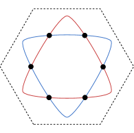
(a)

(b)

Figure 2: Schematics of the Fermi surface. Blue and red correspond to different valleys. Regardless of band structure details, these Fermi surfaces display two prominent features: the symmetry-imposed intersection points between the Fermi surfaces from the two valleys (the valley hot-spots, highlighted with black dots in panel (a)), and the proximity to a van Hove singularity for appropriate doping levels (the van Hove hot-spots, highlighted with grey dots in panel (b)). Valley hot-spots are located along the $\bar{\Gamma}-\bar{K}$ and $\bar{\Gamma}-\bar{K}^{\prime}$ lines, whereas the van Hove hot-spots are located along the $\bar{\Gamma}-\bar{M}$ lines of the moiré Brillouin zone.

At the same one-loop order, the mass of the spin-valley coupled fluctuations also gets enhanced by the same mechanism. These fluctuations couple to the same valley hot-spot via $\sum_{i}\phi_{sv}^{i,1}\Psi^{\dagger}\sigma_{i}\tau_{1}\Psi+\phi_{sv}^{i,2}\Psi^{\dagger}\sigma_{i}\tau_{2}\Psi$. Since the dispersion is spin-degenerate, the renormalization of the corresponding mass term $r_{sv}$ is the same as that for $r_{v}$. Thus, the fluctuations corresponding to $\phi_{sv}$ also get enhanced. At one-loop level, the inter-valley and spin-valley coupled fluctuations are therefore degenerate. But such a degeneracy is not protected by any symmetry, and can be lifted by other effects, such as small perturbations at high energies. For this reason, we will consider $\phi_{v}$ and $\phi_{sv}$ separately.

Aside from the generic considerations above, the proximity to van Hove singularities (and higher-order van Hove singularities) of the FS has been argued to play an important role, particularly for certain electronic concentrations in the TBG phase diagram LiangPRX2 ; Nandkishore19 ; Chichinadze19 ; DasSarma20 ; Chichinadze20 . The van Hove singularities considered in this work take place when the FSs cross the Brillouin zone boundaries. Near the van Hove singularity, thus, for a FS of a given valley, there are pairs of points separated by a small momentum $\delta\bm{q}$ with parallel velocities and enhanced density of states; right at the van Hove singularity, $\delta\bm{q}\to 0$. We denote these pairs of points van Hove hot-spots, as shown in Fig. 2(b). The components of the SU(4) bosonic field $\hat{\Phi}$ that couple to the van Hove hot-spots are the intra-valley ones, which form two three-component fields $\phi_{s}\equiv\phi_{0,i\neq 0}$ and $\phi_{sc}\equiv\phi_{3,i\neq 0}$, as well as a single component field $\phi_{vf}\equiv\phi_{30}$. Clearly, $\phi_{s}$ describes a ferromagnetic order parameter, and, due to the additional valley component, $\phi_{sc}$ describes a spin-current order parameter, breaking spin-rotation and $C_{2z}$ but not time-reversal symmetry. On the other hand, $\phi_{vp}$ corresponds to a valley-polarization order, breaking $C_{2z}$ and time-reversal.

In the case of $\phi_{s}$, the van Hove hot-spots primarily exchange (intra-valley) ferromagnetic spin fluctuations via the coupling term $g\phi_{s}^{i}\Psi^{\dagger}\sigma_{i}\Psi$. Within one-loop, both the mass term $r_{s}$ and the stiffness term $\beta_{s}\delta\bm{q}^{2}$ corresponding to $\phi_{s}$ are renormalized according to

$$r_{s}+\beta_{s}\delta\bm{q}^{2} =r+\beta\delta\bm{q}^{2}$$

$$+g^{2}\sum_{n,\omega_{m}}\int d\bm{k}\frac{1}{i\omega_{m}-{\epsilon}^{n}(\bm{k})}\frac{1}{i\omega_{m}-{\epsilon}^{n}(\bm{k}+\delta\bm{q})}$$ (6)

where ${\epsilon}^{n}(\bm{k})$ corresponds to the dispersion expanded around the $n$-th pair of van Hove hot-spots. Because the Fermi velocities are opposite within a pair of van Hove hot-spots, the mass term $r_{s}$ and the stiffness $\beta_{s}$ are suppressed by the one-loop contribution. At the van Hove singularity, $\delta\bm{q}\rightarrow 0$, the density of states diverges and the Fermi surface becomes non-analytic. The precise form of the $\phi_{s}$ propagator depends on details of the van Hove singularity, which we do not pursue here. In any case, due to the enhanced density of states, near a van Hove singularity, one expects that the enhancement of ferromagnetic fluctuations will be larger than the enhancement in the inter-valley and spin-valley coupled channels discussed above. We also note that the proximity to a van Hove singularity on its own may favor other weak-coupling instabilities that can break translational symmetries, as discussed e.g. in LiangPRX2 ; Chichinadze20 ; here, our focus is instead on how the van Hove singularity lifts the degeneracy of the SU(4) fluctuations that arise from strong-coupling physics.

In the cases of $\phi_{sc}$ and $\phi_{vp}$, i.e., the spin-current and valley-polarized orders, fermions interact with the bosons via the coupling $g\phi_{sc}^{i}\Psi^{\dagger}\tau_{3}\sigma_{i}\Psi$ and $g\phi_{vp}\Psi^{\dagger}\tau_{3}\Psi$. Their corresponding mass terms get renormalized downwards in the same way as in Eq. (6). As a result, $\phi_{sc}$ and $\phi_{vp}$ fluctuations get enhanced in the same manner as those of $\phi_{s}$, at least at one-loop order. However, because they are not related by any symmetry, effects beyond one-loop can lift their degeneracy. For this reason we treat them separately when analyzing the pairing instabilities.

IV Pairing states mediated by SU(4) fluctuations

Having established the dominant ferro-SU(4) fluctuation channels, we now analyze the pairing states favored by the exchange of such fluctuations between low-energy fermions. Fluctuations with small momentum transfer can typically favor multiple superconducting orders with different pairing symmetries; examples include the case of nematic fluctuations Lederer15 ; Kang16 ; Klein19 , ferroelectric fluctuations KoziiFu ; WangCho ; Gastiasoro20 , and charge-order fluctuations with small momentum WangChubukovCF . We will thus focus mainly on the internal structure of the pairing state and determine its spatial dependence based solely on symmetry and energetic argumens. Specifically, when multiple gap functions solve the same gap equation, we will focus only on those gap structures that are nodeless, since a fully gapped state is generally expected to be energetically favored over a nodal state by maximizing the condensation energy.

Generically, with spin and valley degrees of freedom, the SC order parameter couples to fermions via $\hat{\Delta}\Psi^{\dagger}(\bm{k})\Psi^{\dagger T}(-\bm{k})$. We can restrict the form of the possible SC orders by energetics and symmetry arguments. The $D_{6}$ symmetry group acts on both momentum space and valley space; due to the absence of spin-orbit coupling, it acts trivially on spin space. In particular, the two valleys $K$ and $K^{\prime}$ are exchanged under $C_{2x}$ and $C_{2z}$ (see Table 2). Since low-energy fermions at $\bm{k}$ and $-\bm{k}$ necessarily come from two different valleys, we consider Cooper pairing between the two valleys only. As a result, the SC terms are inter-valley ones, which can further be distinguished by “parity”, i.e. the eigenvalues of $C_{2z}$, which takes $\left(k_{x},k_{y}\right)$ to $\left(-k_{x},-k_{y}\right)$. For an even-parity (spin-singlet) order parameter, the pairing vertex is given by

$$\hat{\Delta}=\left[\Delta_{o}(\bm{k})i\tau_{2}+\Delta_{e}(\bm{k})\tau_{1}\right](i\sigma_{2}),$$ (7)

and for an odd-parity (spin-triplet) order parameter

$$\hat{\Delta}^{\prime}_{j}=\left[\Delta^{\prime}_{e}(\bm{k})i\tau_{2}+\Delta^{\prime}_{o}(\bm{k})\tau_{1}\right](\sigma_{j}\,i\sigma_{2}),$$ (8)

where $\Delta_{e}$ and $\Delta^{\prime}_{e}$ are even functions of momentum while $\Delta_{o}$ and $\Delta^{\prime}_{o}$ are odd. The $i\tau_{2}$ term, which is odd under $C_{2z}$, corresponds to valley-singlet pairing, whereas the $\tau_{1}$ term, which is even under $C_{2z}$, corresponds to valley-triplet. Since the SU(2) valley symmetry is broken by the FS, in general both terms appear.

Within the $D_{6}$ point group of TBG considered here, even-parity superconducting order parameters must transform according to the irreducible representations $A_{1},A_{2},E_{2}$, whereas odd-parity ones transform according to the irreps $B_{1},B_{2},E_{1}$. The $A_{1,2}$ and $B_{1,2}$ irreps are one-dimensional while the $E_{1,2}$ irreps are two-dimensional. It is common in the literature to associate a SC state transforming as an irrep of a point group to an orbital angular momentum $s$, $p$, $d$, etc. This is usually done by identifying the spherical harmonic corresponding to the lowest-order basis function of that irrep. Then, $A_{1}$ corresponds to $s$-wave, $A_{2}$ to $i$-wave, $B_{1}$ to $f_{x\left(x^{2}-3y^{2}\right)}$-wave (hereafter denoted $f^{\prime}$-wave for simplicity), $B_{2}$ to $f_{y\left(3x^{2}-y^{2}\right)}$-wave (hereafter denoted $f$-wave for simplicity), $E_{1}$ to $(p_{x},\,p_{y})$-wave, and $E_{2}$ to $(d_{x^{2}-y^{2}},\,d_{xy})$-wave.

The corresponding irrep of an order parameter of the form of Eqs. (7,8) is a product of its irreps in both $\bm{k}$-space and in valley space. In valley space, as shown in Table 2, valley-triplet order $\tau_{1}$ transforms as the $A_{1}$ irrep (i.e. the gap does not change sign upon either a $C_{2z}$ or $C_{2x}$ rotation), whereas valley-singlet order $i\tau_{2}$ transforms as the $B_{2}$ irrep (i.e. the gap changes sign upon either a $C_{2z}$ or $C_{2x}$ rotation).

To determine the leading SC instabilities, one needs to solve the linearized pairing gap equation

$$\hat{\Delta}(\omega,\bm{k})=\sum_{i,\omega^{\prime},\bm{k}^{\prime}} D(\omega-\omega^{\prime},\bm{k}-\bm{k}^{\prime})\Lambda^{i}\hat{G}(\omega^{\prime},\bm{k}^{\prime})$$

$$\times\hat{\Delta}(\omega^{\prime},\bm{k}^{\prime})\hat{G}^{T}(-\omega^{\prime},-\bm{k}^{\prime})\Lambda^{iT}$$ (9)

where $\{\Lambda^{i}\}$ are the pertinent boson-fermion couplings — e.g., for inter-valley fluctuations we have $\{\Lambda^{i}\}=\{\tau_{1},\tau_{2}\}$. Here, $D(\omega-\omega^{\prime},\bm{k}-\bm{k}^{\prime})$ is the bosonic propagator multiplied by $g^{2}$ and renormalized by the boson-fermion coupling, and $\hat{G}(\omega,\bm{k})=\left[i\omega-\hat{\epsilon}(\bm{k})\right]^{-1}$, in matrix form, is the fermionic Green’s function. Because here we are only interested in the momentum and spin/valley structure of the gap function, for simplicity we take the kernel of the gap equation to be diagonal in frequency and assume $\hat{\Delta}(\omega,\bm{k})=\hat{\Delta}(\bm{k})$.

IV.1 Inter-valley channel, $\phi_{v}$

First, we focus on the pairing problem when the dominant fluctuations are in the inter-valley channel, corresponding to either of the two scalar bosonic fields that form $\phi_{v}=\left(\phi_{10},\phi_{20}\right)$ introduced in Sec. III. In this case, we have $\{\Lambda^{i}\}=\{\tau_{1}\sigma_{0},\tau_{2}\sigma_{0}\}$ in Eq. (9). Before solving Eq. (9), it is instructive to convert the effective interaction $-D(k-p)\sum_{i=1,2}\left[\Psi^{\dagger}(k)\tau_{i}\Psi(p)\right]\left[\Psi^{\dagger}(-k)\tau_{i}\Psi(-p)\right]$ to the particle-particle channel to determine for which pairing symmetry the interaction is attractive. To this end, we use the following Fierz identity for the particle-hole channel Joern2018

$$\sum_{i=1,2}(\tau_{i})_{\alpha\beta}(\tau_{i})_{\mu\nu}=(\tau_{1})_{\alpha\mu}(\tau_{1}^{T})_{\nu\beta}-(i\tau_{2})_{\alpha\mu}(i\tau_{2}^{T})_{\nu\beta}.$$ (10)

Plugging it into the effective interaction, we find

$$-D(k-p)\sum_{i=1,2}\left[\Psi^{\dagger}(k)\tau_{i}\Psi(p)\left]\right[\Psi^{\dagger}(-k)\tau_{i}\Psi(-p)\right]$$

$$={-}D(k-p)\left[\Psi^{\dagger}(k)\tau_{1}\Psi^{\dagger T}(-k)\left]\right[\Psi^{T}(-p)\tau_{1}\Psi(p)\right]$$

$${+}D(k-p)\left[\Psi^{\dagger}(k)i\tau_{2}\Psi^{\dagger T}(-k)\left]\right[\Psi^{T}(-p)i\tau_{2}^{T}\Psi(p)\right].$$ (11)

Therefore, the pairing interaction mediated by inter-valley fluctuations is attractive in the valley-triplet channel and repulsive in the valley-singlet channel, analogous to the case of spin ferromagnetic fluctuations. However, as we mentioned above, from a symmetry point of view the valley singlet and triplet channels are always mixed.

To determine the composition of valley singlet and triplet components, we go back to Eq. (9) and inserting the Fierz identity (10), and obtain

$$\hat{\Delta}(\omega,\bm{k})=\frac{1}{2}\sum_{\omega,\bm{k}}D(\omega-\omega^{\prime},\bm{k}-\bm{k}^{\prime})$$

$$\times\left\{\tau_{1}\operatorname{Tr}\left[\tau_{1}\hat{G}(\omega^{\prime},\bm{k}^{\prime})\hat{\Delta}(\omega^{\prime},\bm{k}^{\prime})\hat{G}(-\omega^{\prime},-\bm{k}^{\prime})\right]\right.$$

$$\left.-i\tau_{2}\operatorname{Tr}\left[i\tau_{2}^{T}\hat{G}(\omega^{\prime},\bm{k}^{\prime})\hat{\Delta}(\omega^{\prime},\bm{k}^{\prime})\hat{G}(-\omega^{\prime},-\bm{k}^{\prime})\right]\right\}$$ (12)

If our system had valley SU(2) symmetry, $\hat{G}$ would be proportional to the identity matrix. In this case, the valley-triplet solution with $\hat{\Delta}\propto\tau_{1}$ would be the eigenvector corresponding to the leading pairing channel. The valley-singlet pairing channel, $\hat{\Delta}\propto i\tau_{2}$, would only have the trivial solution $\hat{\Delta}=0$ due to the minus sign in the second term inside the brackets.

Our band dispersion, however, does not have valley SU(2) symmetry. Thus, one needs to solve (12) as a matrix equation and find its eigenvectors, which in general will be a mixture of valley-singlet and valley-triplet. Nonetheless, since we expect $\hat{\Delta}(\bm{k})$ to be peaked around the valley hot-spots [see Fig. 2(a)], where the fermions from the two valleys are degenerate, the problem can be simplified. Let us focus on one valley hot spot, around which we assume the pairing gap has a very weak dependence on $\bm{k}$. From Eq. (4), the Green’s function can be written as

$$\hat{G}(\omega,\pm\bm{k})= \begin{pmatrix}{i\omega-\epsilon_{K}(\bm{k})}&0\\ 0&{i\omega-\epsilon_{K}^{\prime}(\bm{k})}\end{pmatrix}^{-1}=-\frac{i\omega+\epsilon_{+}\pm\epsilon_{-}\tau_{3}}{(i\omega-\epsilon_{+})^{2}-\epsilon_{-}^{2}}$$ (13)

where $\epsilon_{\pm}=\left[\epsilon_{K}(\bm{k})\pm\epsilon_{K^{\prime}}(\bm{k})\right]/2$. Near the hot-spots, we linearize the dispersion $\epsilon_{K}(\bm{k})=\bm{v}_{F}\cdot\bm{k}$, such that the momentum integral becomes $c\int d\epsilon_{+}d\epsilon_{-}$, where the constant $c$ is the Jacobian of the transformation. Within this approximation, one can verify that the valley-triplet pairing solution $\hat{\Delta}(\omega,\bm{k})=\Delta(\omega)\tau_{1}$ remains an eigenvector:

$$\Delta(\omega)\tau_{1}= {c}\sum_{\omega}\int d\epsilon_{+}d\epsilon_{-}\Delta(\omega^{\prime})D(\omega-\omega^{\prime},\bm{k}-\bm{k}^{\prime})\left\{\tau_{1}\operatorname{Tr}\left[\tau_{1}\frac{i\omega^{\prime}+\epsilon_{+}+\epsilon_{-}\tau_{3}}{(i\omega-\epsilon_{+})^{2}-\epsilon_{-}^{2}}\tau_{1}\frac{-i\omega^{\prime}+\epsilon_{+}-\epsilon_{-}\tau_{3}}{(-i\omega-\epsilon_{+})^{2}-\epsilon_{-}^{2}}\right]\right.$$

$$\left.-i\tau_{2}\operatorname{Tr}\left[i\tau_{2}^{T}\frac{i\omega^{\prime}+\epsilon_{+}+\epsilon_{-}\tau_{3}}{(i\omega-\epsilon_{+})^{2}-\epsilon_{-}^{2}}\tau_{1}\frac{-i\omega^{\prime}+\epsilon_{+}-\epsilon_{-}\tau_{3}}{(-i\omega-\epsilon_{+})^{2}-\epsilon_{-}^{2}}\right]\right\}$$

$$= {2c}\sum_{\omega}\int d\epsilon_{+}d\epsilon_{-}\Delta(\omega^{\prime})D(\omega-\omega^{\prime},\bm{k}-\bm{k}^{\prime})(\tau_{1})\left[\frac{\omega^{\prime 2}+\epsilon_{+}^{2}+\epsilon_{-}^{2}}{\left(\omega^{2}+(\epsilon_{+}+\epsilon_{-})^{2}\right)\left(\omega^{2}+(\epsilon_{+}+\epsilon_{-})^{2}\right)}\right]$$

$$= 2c\sum_{\omega^{\prime},\bm{k}^{\prime}}{\Delta}(\omega^{\prime})\tau_{1}\,D(\omega-\omega^{\prime},\bm{k}-\bm{k}^{\prime})\left[\frac{1}{\omega^{\prime 2}+\left(\epsilon_{\bm{K}}(\bm{k})\right)^{2}}+\frac{1}{\omega^{\prime 2}+\left(\epsilon_{\bm{K}^{\prime}}(\bm{k})\right)^{2}}\right]$$ (14)

Note that the $i\tau_{2}\operatorname{Tr}\left(\cdots\right)$ term in the first line, which would have given a mixture with valley-singlet, vanishes after the momentum integration, since the trace is odd in $\epsilon_{-}$ ; this is approximately true when linearizing the dispersion. The integration leads to the standard Cooper logarithmic instability in the valley-triplet channel. The same calculation in the valley-singlet channel yields only the trivial solution $\Delta=0$.

(a)

(b)

Figure 3: Illustration of the $E_{1}$ ($p\pm ip$) [panel (a)] and $E_{2}$ ($d\pm id$) [panel (b)] valley-triplet pairing states mediated by inter-valley flucutations.

Going back to Eqs. (7) and (8), the full symmetry of the pairing order parameter depends on its structure in the spin sector. If it is spin-singlet, restricting the analysis to fully gapped states only, it can be of $A_{1}$ ($s$-wave) or $E_{2}$ ($d$-wave) symmetry; if it is spin-triplet, the fully gapped state corresponds to a $E_{1}$ ($p$-wave) pairing. Because the valley-triplet component of the gap, $\tau_{1}$, transforms trivially under $D_{6}$ (i.e. as the $A_{1}$ irrep), the $\bm{k}$-space structure of the gap solely determines the irrep of the order parameter. Energetically, it is natural to expect that $\Delta_{o}\sim(\cos\theta,\pm i\sin\theta)$ for the $E_{1}$ state (yielding a $p\pm ip$ state) and $\Delta_{e}\sim(\cos 2\theta,\pm i\sin 2\theta)$ for the $E_{2}$ state (yielding a $d\pm id$ state) to ensure a fully gapped state, where $\theta$ is a polar angle parametrizing the FS (without loss of generality, in the ensuing discussion we will choose the plus sign). We illustrate the $p+ip$ and $d+id$ SC gaps corresponding to these $E_{1}$ and $E_{2}$ pairing states in Fig. 3; the arrows correspond to the direction of $\Delta_{o,e}$ in the two-dimensional space of their corresponding irrep $E_{1,2}$. Since the winding on the two valley FSs are the same, these are both chiral states that also break time-reversal symmetry. From the winding numbers of the gap functions on the FS, the Chern number of the $E_{2}$ state is $C=4$ (using the convention that a spinless $p+ip$ superconductor has Chern number $C=1/2$ due to the redundancy of the Bogoliubov-de-Gennes Hamiltonian liu-2018 ), whereas for the $E_{1}$ state it is $C=2$. On the other hand, the $A_{1}$ state has a Chern number $C=0$. Note that topological SC in TBG was previously proposed within different models Leon1 .

Note that the inter-valley fluctuations do not directly distinguish the strengths of spin-singlet and spin-triplet pairing tendencies. Moreover, the pairing interaction is peaked at small momentum transfer, which is known to favor multiple nearly degenerate pairing orders Kivelson ; Gastiasoro20 . We thus expect all three pairing instabilities to be close competitors. Which order is the true leading instability requires additional details beyond the scope of our model, such as the correlation length of the nematic fluctuations and the fermionic band dispersion. Extrinsic factors such as disorder also could also lift this near-degeneracy, likely favoring the time-reversal symmetric $A_{1}$ state.

IV.2 Spin-valley coupled channel, $\phi_{sv}$

We now consider spin-valley coupled fluctuations, which are associated with either of the two vector bosonic fields $\phi_{sv}=\left(\phi_{1i\neq 0},\phi_{2i\neq 0}\right)$ (see Sec. III). The pairing gap equation is still given by Eq. (9), but now with $\{\Lambda^{i}\}=\{\bm{\sigma}\tau_{1},\bm{\sigma}\tau_{2}\}$. Just like in the $\phi_{v}$ case, although the gap function is a mixture between valley-singlet and valley-triplet, near the valley hot-spots the valley singlet/triplet assignment remains approximately valid. To determine the leading attractive pairing, we start from the Fierz identities:

$$\sum_{i=1,2}(\tau_{i})_{\alpha\beta}(\tau_{i})_{\mu\nu}=(\tau_{1})_{\alpha\mu}(\tau_{1})_{\nu\beta}-(i\tau_{2})_{\alpha\mu}(i\tau_{2}^{T})_{\nu\beta}.$$

$$(\bm{\sigma})_{\gamma\delta}\cdot(\bm{\sigma})_{\rho\lambda}=\frac{1}{2}(\bm{\sigma}i\sigma_{2})_{\gamma\rho}\cdot(i\sigma_{2}^{T}\bm{\sigma}^{T})_{\lambda\delta}-\frac{3}{2}(i\sigma_{2})_{\gamma\rho}(i\sigma_{2}^{T})_{\lambda\delta}$$ (15)

Taking the direct product, we find:

$$-D(k-p)\sum_{i=1,2}\left[\Psi^{\dagger}(k)\tau_{i}\bm{\sigma}\Psi(p)\left]\cdot\right[\Psi^{\dagger}(-k)\tau_{i}\bm{\sigma}\Psi(-p)\right]$$

$$= -\frac{3}{2}D(k-p)\left[\Psi^{\dagger}(k)i\sigma_{2}i\tau_{2}\Psi^{\dagger T}(-k)\left]\right[\Psi(p)i\tau_{2}^{T}i\sigma_{2}^{T}\Psi^{T}(-p)\right]$$

$$-\frac{1}{2}D(k-p)\left[\Psi^{\dagger}(k)(i\bm{\sigma}\sigma_{2})(\tau_{1})\Psi^{\dagger T}(-k)\right]$$

$$~{}~{}~{}~{}~{}~{}~{}~{}\times\left[\Psi(p)(\tau_{1})(i\sigma_{2}^{T}\bm{\sigma}^{T})\Psi^{T}(-p)\right]$$

$$+\frac{3}{2}D(k-p)\left[\Psi^{\dagger}(k)i\sigma_{2}(\tau_{1})\Psi^{\dagger T}(-k)\right]$$

$$~{}~{}~{}~{}~{}~{}~{}~{}\times\left[\Psi(p)(\tau_{1})i\sigma_{2}^{T}\Psi^{T}(-p)\right]$$

$$+\frac{1}{2}D(k-p)\left[\Psi^{\dagger}(k)(i\bm{\sigma}\sigma_{2})\tau_{3}\Psi^{\dagger T}(-k)\right]$$

$$~{}~{}~{}~{}~{}~{}~{}~{}\times\left[\Psi(p)\tau_{3}(i\sigma_{2}^{T}\bm{\sigma}^{T})\Psi^{T}(-p)\right]$$ (16)

Therefore, the most attractive (i.e. negative in the above equation) interaction is in the spin-singlet, valley-singlet channel. Note that there is also sub-leading attraction in one spin-triplet valley-triplet channel, but repulsion in the spin-singlet valley-triplet channel and in another spin-triplet valley-triplet channel.

(a)

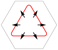
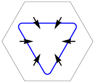
(b)

Figure 4: Illustration of the $A_{2}$ ($i$-wave) [panel (a)] and $E_{2}$ ($d\pm id$) [panel (b)] valley-singlet pairing states mediated by spin-valley flucutations.

By solving the gap equation with a valley-split Green’s function like we did in Eq. (14), we confirm that indeed the leading pairing instability is towards a spin-singlet, valley-singlet channel. From Eq. (7), we see that this is an even-parity superconducting gap with a dominant odd spatial function $\Delta_{o}(\bm{k})$. There are thus three choices, $\Delta_{o}\sim\cos\theta,\sin\theta,\cos 3\theta$; note that the gap function $\sin 3\theta$ vanishes on the valley hot spots, and thus can be discarded. The first two choices for $\Delta_{o}$ give rise to a gap function that transforms as the two-dimensional irrep $E_{2}$ (i.e. $d$-wave); the resulting superconducting state is fully gapped if the chiral “$d+id$” solution is realized, $\Delta_{o}\sim\left(\cos\theta,\,i\sin\theta\right)$. To see that the total gap function transforms as $E_{2}$, note that $\Delta_{o}\sim\left(\cos\theta,\,i\sin\theta\right)$ transforms as the $E_{1}$ irrep, and that the valley component $i\tau_{2}$ transforms as the $B_{2}$ irrep. The irrep associated with the full gap is thus obtained by combining the valley and spatial components using the product $E_{1}\otimes B_{2}=E_{2}$. If, on the other hand, $\Delta_{o}\sim\cos 3\theta$ is selected, the total gap function transforms as the irrep $A_{2}$ ($i$-wave). This follows from the fact that $\cos 3\theta$ transforms as the $B_{1}$ irrep and that $B_{1}\otimes B_{2}=A_{2}$. Note that a similar $i$-wave gap was previously proposed in another study on TBG Chichinadze19 . While a single-band $i$-wave order has 12 nodes, our $A_{2}$ order parameter has six nodes per valley FS, located between the valley hot-spots. We illustrate the pairing orders $A_{2}$ and $E_{2}$ in Fig. 4. Note that for $E_{2}$ in Fig. 4(b), the windings on the two FS’s are the same, thus breaking time-reversal symmetry. Although it has the same symmetry as a $d+id$ state, the winding number of $\Delta_{o}\sim\left(\cos\theta,\,i\sin\theta\right)$ is one, suggesting that the total Chern number is $C=2$ (including two valleys). The gapless $A_{2}$ pairing state does not have a well-defined Chern number due to the existence of nodes. As before, to further select between the two pairing instabilities, additional microscopic details must be considered. For example, disorder effects are expected to favor the fully gapped $E_{2}$ state over the nodal $A_{2}$ state.

IV.3 Ferromagnetic channel, $\phi_{s}$

In the case of enhanced ferromagnetic fluctuations $\phi_{s}$ near a van Hove singularity, the linearized gap equation is given by (9) with $\{\Lambda_{i}\}=\{\bm{\sigma}\}$. Using the second line of Eq. (15) we find that the leading instability is in the spin-triplet channel $\hat{\Delta}\propto\bm{\sigma}i\sigma_{2}$ and thus the favored pairing channel is of odd-parity. The relevant odd parity irreps of $D_{6}$ are $E_{1}$ ($p$-wave) and $B_{1,2}$ ($f$-wave).

The $E_{1}$ irrep is two-dimensional, and depending on the gap structure in the valley sector, there are two choices for the $\bm{k}$ dependence of the gap function that are fully gapped ($p\pm ip$ state): $\Delta_{o}^{\prime}\sim\left(\cos\theta,\,i\sin\theta\right)$, and $\Delta_{e}^{\prime}\sim\left(\cos 2\theta,\,i\sin 2\theta\right)$. To see this, we notice that $\Delta_{o}^{\prime}$ transforms as $E_{1}$, and the triplet valley component $\tau_{1}$ transforms as $A_{1}$; on the other hand, $\Delta^{\prime}_{e}$ transforms as $E_{2}$, and the valley-singlet component $i\tau_{2}$ transforms as $B_{2}$, resulting in a $E_{1}$ total gap since $E_{2}\otimes B_{2}=E_{1}$. Because $\Delta^{\prime}_{o}$ has opposite signs on the two van Hove hot-spots [see Fig. 5], this configuration is expected to be energetically disfavored and thus subleading to $\Delta^{\prime}_{e}$, which is shown in Fig. 6(a). However, because $\Delta_{e}^{\prime}$ and $\Delta_{o}^{\prime}$ result in a gap with the same $E_{1}$ symmetry, they are always mixed. Since their winding number on each FS is different, the Chern number of the resulting SC order depends on whether $\Delta^{\prime}_{o}$ or $\Delta^{\prime}_{e}$ dominates. For our case $|\Delta^{\prime}_{e}|>|\Delta^{\prime}_{o}|$, in each triangular FS the phase of the order parameter winds twice, like a $d+id$ order, despite the fact that the symmetry of the pairing state is identical to $p+ip$. As a result, the total Chern number should be $4$, coming from $C=2$ for two spin species.

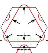
Figure 5: The structure of $\Delta^{\prime}_{o}$ for the case of valley-triplet, spin-triplet $p+ip$ pairing mediated by ferromagnetic fluctuations. Note the sign change between a pair of van Hove hot-spots.

As for the case of a gap transforming as either the $B_{1}$ or $B_{2}$ irrep, it is possible to construct a fully gapped valley-singlet $B_{2}$ state with $\Delta^{\prime}_{e}\sim\textrm{const}$, since $i\tau_{2}$ transforms as $B_{2}$. For energetic reasons, we expect this gap to be favored over the other possible combinations. The full gaps on the two valley FSs have opposite signs, since this is a valley-singlet state, as shown in Fig. (6)(b). Superimposing the two Fermi surfaces, the gap indeed has the $\sin 3\theta$ variation across the Brillouin zone characteristic of a $B_{2}$ $f$-wave gap, yet the state is fully gapped. This pairing state has a Chern number $C=0$.

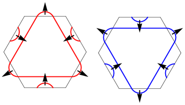
(a)

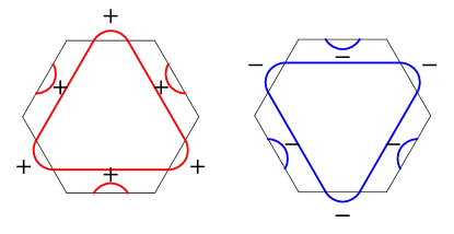
(b)

Figure 6: Illustration of the $E_{1}$ ($p\pm ip$) [panel (a)] and $B_{2}$ ($f$-wave) [panel (b)] spin-triplet pairing states mediated by the ferromagnetic flucutations.

It is interesting to consider how disorder effects distinguish the two pairing states. Assuming each graphene sheet is atomically clean, disorder in TBG occurs at the the moiré length scale, for example, from a variation of the twist angle. Scattering by impurities at the moiré length scale has small (atomic lattice) momentum transfer and preserves valley index. Since the $B_{2}$ pairing gap does not change sign within a valley, we expect it to be more robust than $E_{1}$ order against such long distance disorder.

IV.4 Spin-current channel, $\phi_{sc}$

We now consider the fluctuations associated with the spin-current state, described by the vector bosonic field $\phi_{sc}=\phi_{3i\neq 0}$. As we discussed, this bosonic field couples to the fermions via $\Lambda_{i}=\tau_{3}\sigma_{i}$. Performing a similar calculation to Eq. (18), we find that the leading pairing instability remains in the spin-singlet channel. This follows from the Fierz identities

$$(\tau_{3})_{\alpha\beta}(\tau_{3})_{\mu\nu}= \frac{1}{2}(\tau_{3})_{\alpha\mu}(\tau_{3})_{\nu\beta}+\frac{1}{2}(\tau_{0})_{\alpha\mu}(\tau_{0})_{\nu\beta}$$ (17)

$$-\frac{1}{2}(\tau_{1})_{\alpha\mu}(\tau_{1})_{\nu\beta}-\frac{1}{2}(i\tau_{2})_{\alpha\mu}(i\tau_{2}^{T})_{\nu\beta}$$

$$(\bm{\sigma})_{\gamma\delta}\cdot(\bm{\sigma})_{\rho\lambda}= \frac{1}{2}(\bm{\sigma}i\sigma_{2})_{\gamma\rho}\cdot(i\sigma_{2}^{T}\bm{\sigma}^{T})_{\lambda\delta}-\frac{3}{2}(i\sigma_{2})_{\gamma\rho}(i\sigma_{2}^{T})_{\lambda\delta}$$

Taking a direct product, the fermion interaction can be rewritten as

$$-D(k-p)\left[\Psi^{\dagger}(k)\tau_{3}\bm{\sigma}\Psi(p)\left]\cdot\right[\Psi^{\dagger}(-k)\tau_{3}\bm{\sigma}\Psi(-p)\right]=$$

$$-\frac{3}{4}D(k-p)\left[\Psi^{\dagger}(k)i\sigma_{2}\tau_{1}\Psi^{\dagger T}(-k)\left]\right[\Psi(p)\tau_{1}^{T}i\sigma_{2}^{T}\Psi^{T}(-p)\right]$$

$$-\frac{3}{4}D(k-p)\left[\Psi^{\dagger}(k)i\sigma_{2}i\tau_{2}\Psi^{\dagger T}(-k)\left]\right[\Psi(p)i\tau_{2}^{T}i\sigma_{2}^{T}\Psi^{T}(-p)\right]$$

$$+\cdots$$ (18)

where $\cdots$ stand for terms with less negative (including positive) coefficients corresponding to channels with weaker attraction or repulsion. It is clear that the leading attractive channel for pairing is the spin-singlet channel. From Eq. (7), this corresponds to an even-parity state. As before, the $\Delta_{e}\tau_{1}$ and $\Delta_{o}i\tau_{2}$ components are always mixed. Now, the valley-singlet pairing $i\tau_{2}$, which transforms as $B_{2}$, requires $\Delta_{o}\sim\left(\cos\theta,\,i\sin\theta\right)$, which transforms as $E_{1}$, resulting in the even-parity gap $E_{2}$. However, $\Delta_{o}$ changes sign within a pair of van Hove hot-spots (see Fig. 5). Since pairing is driven by the pairs of van Hove hot-spots, we conclude that the energetically dominant component is valley triplet and spin singlet ($\Delta_{e}\tau_{1}$), mixed with a small valley singlet component. Since $\tau_{1}$ transforms as $A_{1}$, $\Delta_{e}$ can either be a constant, resulting in an $s$-wave gap, or $\Delta_{o}\sim\left(\cos 2\theta,\,i\sin 2\theta\right)$, resulting in a $d$-wave gap. We illustrate these two pairing states on the FSs in Fig. 7. Compared with those promoted by ferromagnetic fluctuations, the pairing gaps driven by spin-current fluctuations have similar structures within an individual FS but differ by parity. From their windings on the FS, the Chern numbers for the $s$-wave state and $d$-wave state are $C=0$ and $C=4$, respectively. At the hot-spots level, the $s$-wave and $d$-wave orders are degenerate. However, when the full FS and/or disorder effects are taken into account, it is likely that the fully gapped $s$-wave order becomes the dominant one.

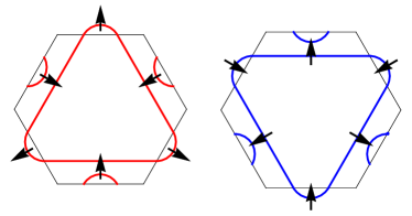
(a)

(b)

Figure 7: Illustration of $E_{2}$ ($d\pm id$) [panel (a)] and the $A_{1}$ ($s$-wave) [panel (b)] spin-singlet pairing states mediated by spin-current fluctuations.

IV.5 Valley-polarized channel, $\phi_{vp}$

Finally, we analyze the pairing instabilities driven by fluctuations in the valley-polarized channel. From the first line of Eq. (17), we see that the fluctuations of the $\phi_{vp}$ field yield attraction in two valley-triplet channels, with pairing orders $\sim\Delta\tau_{0}$ and $\sim\Delta\tau_{3}$. However, both of them correspond to intra-valley pairing. As we mentioned in the beginning of this Section, intra-valley pairing involves FSs that are not invariant under $C_{2z}$, i.e. the $\bm{k}$ and $\bm{-k}$ states are not at the same energy. As a result, the Cooper logarithm is cutoff and does not diverge at zero temperature. Hence, intra-valley pairing is energetically disfavored within the SU(4) spin-valley-fermion model. Therefore $\phi_{vp}$ fluctuations do not induce any superconducting phases, at least within weak-coupling.

V Nematic superconductivity

Recent experiments in TBG have reported that the SC dome near half-filling breaks the $C_{3z}$ rotational symmetry of the moiré superlattice, i.e., it is a nematic superconductor Cao20 ; SigristUeda91 . An interesting question is whether the pairing states that result from the exhange of ferro-SU(4) fluctuations can become nematic. From a symmetry standpoint, the nematic order parameter is a 3-state Potts order parameter that transforms as the $E_{2}$ irrep Fernandes2 . Thus, for a superconducting state to display subsidiary nematic order, a SC bilinear must transform according to $E_{2}$. For an isolated pairing instability, this is only possible for the $E_{1}$ ($p$-wave) and $E_{2}$ ($d$-wave) instabilities, since $E_{1,2}\otimes E_{1,2}=A_{1}\oplus A_{2}\oplus E_{2}$. However, as we discussed above, from energetic arguments one generally expects that the SC ground state associated with the $E_{1,2}$ instabilities will be the chiral one ($p\pm ip$ and $d\pm id$ states), since it fully gaps the Fermi surface. In contrast, the nematic solutions $p\pm p$ and $d\pm d$ generally generate nodes. This is consistent with microscopic calculations discussed elsewhere, which argued that the chiral solution is generally favored over the nematic one Kozii19 . Nevertheless, it has been pointed out that proximity to a separate normal-state nematic instability may tip the balance in favor of the nematic over the chiral state Kozii19 .

Another possibility, which we explore in more details in this section, is that superconducting nematic order can appear when two SC states with different symmetries coexist microscopically. This was previously discussed in the context of the iron pnictide superconductors, where coexistence of $s$-wave and $d$-wave superconductivity gives rise to a nematic SC state FernandesMillis , and also in the context of TBG, where nematic order was shown to arise from the coexistence of $i$-wave and $d$-wave Chichinadze19 . As we discussed in Sec. III, the exchange of ferro-SU(4) fluctuations generally leads to closely competing SC instabilities with different symmetries, which can potentially lead to coexistence between different pairing states. Symmetry restricts the possible combinations of gap functions that can result in a subsidiary nematic order parameter. Quite generally, one needs to combine a state that transforms as a one-dimensional irrep (i.e. $A_{1}$, $A_{2}$, $B_{1}$, $B_{2}$) with another state that transforms as a two-dimensional irrep (i.e. $E_{1}$, $E_{2}$), such that the product of these irreps transforms as $E_{2}$. There are then four possibilities: $A_{1}$ and $E_{2}$ (dubbed $s\pm d$ state), $A_{2}$ and $E_{2}$ ($i\pm d$ state, as in Ref. Chichinadze19 ), $B_{1}$ and $E_{1}$ ($f^{\prime}\pm p$ state), $B_{2}$ and $E_{1}$ ($f\pm p$ state). The fact that these states are nematic follows from the products of irreps of $D_{6}$: $A_{1}\otimes E_{2}=A_{2}\otimes E_{2}=B_{1}\otimes E_{1}=A_{2}\otimes E_{2}=E_{2}$. As shown in Table 1, we find that for each of the ferro-SU(4) channels considered here that induce superconductivity, there is at least one combination of closely competing SC states of different symmetries that can result in an accompanying nematic order. As we mentioned, when two SC order parameters $\Delta_{a,b}$ coexist, the energetically-favored coexisting order parameter is typically of the form $\Delta_{a}\pm i\Delta_{b}$, breaking time-reversal symmetry rather than spatial symmetries. However, as we show below, owing to the internal structure of one of the order parameters (e.g., the $d$-wave above is by itself $d\pm id$), the ground state can indeed be a nematic state in our case.

To illustrate the appearance of nematic order in the coexistence state, we write down the a Ginzburg-Landau theory that describes one the four cases discussed above. The analysis is similar to that done in Ref. Chichinadze19 for the case of coexisting SC orders that transform as the $A_{2}$ and $E$ irreps of the $D_{3}$ point group considered in that work. Here, let $\Delta_{0}$ be the SC order parameter that transforms as the one-dimensional irrep $A_{1}$ and $\boldsymbol{\Delta}_{E}\equiv\left(\Delta{}_{1},\Delta{}_{2}\right)$, the SC order parameter that transforms as the two-dimensional irrep $E_{2}$. Before writing down the SC free-energy expansion, we define the two subsidiary nematic order parameters $\boldsymbol{\varphi}_{0}$ and $\boldsymbol{\varphi}_{E}$ that arise from bilinear combinations of the SC order parameters that transform as the $E_{2}$ irrep:

$$\boldsymbol{\varphi}_{0} =\begin{pmatrix}\Delta_{0}^{*}\Delta_{1}+\Delta_{1}^{*}\Delta_{0}\\ \Delta_{0}^{*}\Delta_{2}+\Delta_{2}^{*}\Delta_{0}\end{pmatrix}$$ (19)

$$\boldsymbol{\varphi}_{E} =\begin{pmatrix}\left|\Delta_{1}\right|^{2}-\left|\Delta_{2}\right|^{2}\\ -\Delta_{1}^{*}\Delta_{2}-\Delta_{1}\Delta_{2}^{*}\end{pmatrix}$$ (20)

We consider the free energy up to the quartic terms of the SC order parameters. The free energy for $\Delta_{0}$ is given by the standard form

$$F_{0}=\frac{\alpha_{0}}{2}|\Delta_{0}|^{2}+\frac{\beta_{0}}{4}|\Delta_{0}|^{4}\ .$$ (21)

As for the free energy for $\boldsymbol{\Delta}_{E}$, invariance under $D_{6}$ and U(1) symmetries give:

$$F_{E} = \frac{\alpha_{E}}{2}\left(\left|\Delta_{1}\right|^{2}+\left|\Delta_{2}\right|^{2}\right)+\frac{\beta_{E}}{4}\left(\left|\Delta_{1}\right|^{2}+\left|\Delta_{2}\right|^{2}\right)^{2}$$ (22)

$$-\frac{\gamma_{EE}}{4}\left|\Delta_{1}^{*}\Delta_{2}-\Delta_{1}\Delta_{2}^{*}\right|^{2}\,.$$

As we discussed above, if only $\boldsymbol{\Delta}_{E}$ SC order is present, the SC order parameter is expected to be of the chiral form $\Delta_{1}\pm i\Delta_{2}$, which breaks time-reversal symmetry while maintaining the $C_{3z}$ rotational symmetry. This implies a positive coefficient $\gamma_{EE}>0$.

The coupling between the SC order parameters, $\Delta_{0}$ and $\boldsymbol{\Delta}_{E}$, up to the quartic order, consists of the following terms

$$F_{0E} = \frac{\lambda}{2}\,|\Delta_{0}|^{2}\left(\left|\Delta_{1}\right|^{2}+\left|\Delta_{2}\right|^{2}\right)$$ (23)

$$+\frac{\gamma_{0E}}{2}\left[\left(\Delta_{0}^{*}\Delta_{1}+\Delta_{0}\Delta_{1}^{*}\right)\left(\left|\Delta_{1}\right|^{2}-\left|\Delta_{2}\right|^{2}\right)\right.$$

$$\left.-\left(\Delta_{0}^{*}\Delta_{2}+\Delta_{2}^{*}\Delta_{0}\right)\left(\Delta_{1}^{*}\Delta_{2}+\Delta_{1}\Delta_{2}^{*}\right)\right]$$

$$+\frac{\gamma_{00}}{4}\left[\left(\Delta_{0}^{*}\right)^{2}\left(\Delta_{1}^{2}+\Delta_{2}^{2}\right)+\mathrm{c.c.}\right]$$

The total free energy $F\equiv F_{0}+F_{E}+F_{E0}$ can be cast in a more transparent form by noting that:

$$\left|\Delta_{1}^{*}\Delta_{2}-\Delta_{1}\Delta_{2}^{*}\right|^{2} =-\left(\left|\Delta_{1}\right|^{2}-\left|\Delta_{2}\right|^{2}\right)^{2}$$ (24)

$$-\left(\Delta_{1}^{*}\Delta_{2}+\Delta_{1}\Delta_{2}^{*}\right)^{2}+\left(\left|\Delta_{1}\right|^{2}+\left|\Delta_{2}\right|^{2}\right)^{2}$$

and that:

$$\left[\left(\Delta_{0}^{*}\right)^{2}\left(\Delta_{1}^{2}+\Delta_{2}^{2}\right)+\mathrm{c.c.}\right] =\left(\Delta_{0}^{*}\Delta_{1}+\Delta_{1}^{*}\Delta_{0}\right)^{2}$$

$$+\left(\Delta_{0}^{*}\Delta_{2}+\Delta_{2}^{*}\Delta_{0}\right)^{2}- 2|\Delta_{0}|^{2}\left(\left|\Delta_{1}\right|^{2}+\left|\Delta_{2}\right|^{2}\right)$$ (25)

Then, we have:

$$F=\left[\frac{\alpha_{0}}{2}|\Delta_{0}|^{2}+\frac{\beta_{0}}{4}|\Delta_{0}|^{4}\right]$$

$$+\left[\frac{\alpha_{E}}{2}\left(\left|\Delta_{1}\right|^{2}+\left|\Delta_{2}\right|^{2}\right)+\frac{\left(\beta_{E}-\gamma_{EE}\right)}{4}\left(\left|\Delta_{1}\right|^{2}+\left|\Delta_{2}\right|^{2}\right)^{2}\right]$$

$$+\frac{\left(\lambda-\gamma_{00}\right)}{2}\,|\Delta_{0}|^{2}\left(\left|\Delta_{1}\right|^{2}+\left|\Delta_{2}\right|^{2}\right)+\delta F$$ (26)

with:

$$\delta F=\frac{1}{4}\left(\begin{array}[]{cc}\boldsymbol{\varphi}_{0}^{T}&\boldsymbol{\varphi}_{E}^{T}\end{array}\right)\cdot\left(\begin{array}[]{cc}\gamma_{00}&\gamma_{0E}\\ \gamma_{0E}&\gamma_{EE}\end{array}\right)\left(\begin{array}[]{c}\boldsymbol{\varphi}_{0}\\ \boldsymbol{\varphi}_{E}\end{array}\right)$$ (27)

Note that $F-\delta F$ is insensitive on the relative phases between the three SC order parameters $\Delta_{0}$, $\Delta_{1}$, and $\Delta_{2}$. All it does is to determine whether there is a coexistence state in which both $\Delta_{0}$, $\boldsymbol{\Delta}_{E}$ are simultaneously non-zero. The symmetry of the coexistence state is determined solely by the minimization of $\delta F$. In this regard, note that $\gamma_{EE}>0$ favors a relative phase of $\pi/2$ between $\Delta_{1}$ and $\Delta_{2}$, which corresponds to $\boldsymbol{\varphi}_{E}=0$; $\gamma_{00}>0$ favors a relative phase of $\pi/2$ between $\Delta_{0}$ and $\Delta_{1},\,\Delta_{2}$, which corresponds to $\boldsymbol{\varphi}_{0}=0$. However, regardless of the sign of $\gamma_{0E}$, it always favors a state in which the two nematic order parameters $\boldsymbol{\varphi}_{E}$ and $\boldsymbol{\varphi}_{0}$ are both non-zero and either parallel ($\gamma_{0E}<0$) or anti-parallel ($\gamma_{0E}>0$).

To find out the nature of the coexistence phase, one needs to diagonalize the matrix in Eq. (27). The eigenvalues are given by:

$$\gamma_{\pm}=\left(\frac{\gamma_{00}+\gamma_{EE}}{2\gamma_{0E}}\right)\pm\sqrt{\left(\frac{\gamma_{00}-\gamma_{EE}}{2\gamma_{0E}}\right)^{2}+1}$$ (28)

and the eigenvectors are given by

$$\boldsymbol{\varphi}_{E}=\left[\left(\frac{\gamma_{00}-\gamma_{EE}}{2\gamma_{0E}}\right)\pm\sqrt{\left(\frac{\gamma_{00}-\gamma_{EE}}{2\gamma_{0E}}\right)^{2}+1}\right]\boldsymbol{\varphi}_{0}$$ (29)

Because $\gamma_{EE}>0$, the eigenvalue $\gamma_{+}$ is always positive. However, $\gamma_{-}$ can be negative if $\gamma_{0E}^{2}>\gamma_{00}\gamma_{EE}$. When this condition is satisfied, the energy is minimized by condensing the auxiliary nematic order parameter $\boldsymbol{\varphi}_{-}$, and the coexistence state becomes a nematic superconductor. Note that $\boldsymbol{\varphi}_{-}$ consists of the two original nematic “vectors” $\boldsymbol{\varphi}_{0}$ and $\boldsymbol{\varphi}_{E}$ aligned parallel to each other, if $\gamma_{0E}<0$, or anti-parallel to each other, if $\gamma_{0E}>0$. A similar condition for the coexistence state to be nematic was also found in Ref. Chichinadze19 for the case of an $A_{2}$ and an $E$ superconducting states. We emphasize that additional cubic term in $\boldsymbol{\varphi}_{0}$ and $\boldsymbol{\varphi}_{E}$, which are allowed by $D_{6}$ symmetry, lower the symmetry of the nematic order parameter from a two-dimensional vector (i.e. an “XY” order parameter) to a 3-state Potts order parameter Fernandes1 ; Fernandes2 .

It is interesting to discuss what happens if $\gamma_{0E}^{2}<\gamma_{00}\gamma_{EE}$. In that case, the $\delta F$ term in the free energy would be minimized by simultaneously vanishing the two auxiliary nematic order parameters $\boldsymbol{\varphi}_{0}$ and $\boldsymbol{\varphi}_{E}$. However, a quick inspection of Eq. (20) shows that this is not possible. On the one hand, for $\boldsymbol{\varphi}_{E}$ to vanish, one needs to impose $\Delta_{1}=\pm i\Delta_{2}$. On the other hand, $\boldsymbol{\varphi}_{0}$ will only vanish if the relative phase between $\Delta_{0}$ and $\Delta_{1}$ and the relative phase between $\Delta_{0}$ and $\Delta_{2}$ are $\pm\pi/2$. Thus, in order for $\boldsymbol{\varphi}_{E}=\boldsymbol{\varphi}_{0}=0$, the three complex fields $\Delta_{0}$, $\Delta_{1}$, and $\Delta_{2}$ must all have relative phases of $\pm\pi/2$ with respect to each other, which is impossible. This situation is analogous to geometrically frustrated antiferromagnetism on a triangular lattice. The outcome is that the relative phases between $\Delta_{0}$, $\Delta_{1}$, and $\Delta_{2}$ will be neither $0,\pi$ nor $\pm\pi/2$. As a result, nematic order will persist even if $\gamma_{0E}^{2}<\gamma_{00}\gamma_{EE}$, however it will generally be accompanied by time-reversal symmetry-breaking Chichinadze19 . In this sense, this order is more appropriately referred to as a chiral-nematic order.

The above analysis focused on the case where the two coexisting SC order parameters were $A_{1}$ and $E_{2}$. Similar expressions can be derived for the other cases discussed in Table 1. Let us denote the $E_{1}$ or $E_{2}$ SC order parameters generically as $\boldsymbol{\Delta}_{E}\equiv\left(\Delta{}_{1},\Delta{}_{2}\right)$, and the $A_{2}$, $B_{1}$, or $B_{2}$ SC order parameter, $\Delta_{0}$. The free energy acquires the same form as Eqs. (26) and (27), with $\boldsymbol{\varphi}_{E}$ still defined by Eq. (20), but $\boldsymbol{\varphi}_{0}$ acquiring different functional forms. In particular, we have

$$\boldsymbol{\varphi}_{0}^{(A_{1},E_{2})/(B_{1},E_{1})} =\begin{pmatrix}\Delta_{0}^{*}\Delta_{1}+\Delta_{1}^{*}\Delta_{0}\\ \Delta_{0}^{*}\Delta_{2}+\Delta_{2}^{*}\Delta_{0}\end{pmatrix}$$ (30)

$$\boldsymbol{\varphi}_{0}^{(A_{2},E_{2})/(B_{2},E_{1})} =\begin{pmatrix}-\Delta_{0}^{*}\Delta_{2}-\Delta_{2}^{*}\Delta_{0}\\ \Delta_{0}^{*}\Delta_{1}+\Delta_{1}^{*}\Delta_{0}\end{pmatrix}$$ (31)

Regardless of the definition of $\boldsymbol{\varphi}_{0}$, the condition for a nematic superconductor to take place in all these coexistence phases is the same as before, $\gamma_{0E}^{2}>\gamma_{00}\gamma_{EE}$.

Although in this section we studied the emergence of nematic order when the system has already developed long-range SC order, it is worth emphasizing that nematic order may be established close to but above the SC transition temperature, as long as the SC fluctuations are strong enough. In this case, the nematic order is understood as a vestigial SC order. A detailed analysis of the vestigial order requires one to go beyond mean-field theory and rewrite the free energy in terms of composite order parameters Vestigial , which we leave for future work.

VI Summary

In this work we analyzed an SU(4) spin-valley-fermion model, in which itinerant fermions in a hexagonal two-band system are coupled to soft fluctuations associated with a large SU(4) symmetry. Previous theoretical studies have largely focused on either weak-coupling approaches or strong-coupling approaches. In the latter, which neglects the kinetic energy, it has been shown that a SU(4) “ferromagnetic-like” order arises. In the former, it has been emphasized the importance of Fermi surface properties such as van Hove singularities, and various symemtry-breaking intertwined orders have been predicted.

While a self-consistent analysis bridging these two approaches is remarkably difficult, our phenomonelogical SU(4) spin-valley-fermion model provides an interesting first step towards this goal. More specifically, this model assumes that the ferro-SU(4) fluctuations arise from energy scales much larger than the bandwidth, and treat them as an input of the theory. The coupling between these ferro-SU(4) fluctuations and the low-energy fermions has two main effects: on the one hand, it partially lifts the huge degeneracy associated with the SU(4) manifold. On the other hand, it gives rise to a rich landscape of superconducting phases with non-trivial topology, nodes, and broken time-reversal symmetry. Superconducting nematicity, as signaled by the spontaneous breaking of the lattice rotational symmetry inside the superconducting state, emerges quite naturally due to the near degeneracy of the competing pairing states, despite the fact that none of the superconducting states are by themselves nematic.

Remarkably, these results are robust despite the lack of a detailed knowledge of the Fermi surface of twisted bilayer graphene, as they only depend on general features of the Fermi surface, namely, the valley hot-spots and the van Hove hot-spots. In this regard, the SU(4) spin-valley-fermion model is the TBG counterpart of the widely-studied SU(2) spin-fermion model usually applied to cuprate superconductors. The main differences are the existence of valley degrees of freedom and the condensation of the SU(4) order parameter in a “ferromagnetic-like” configuration, i.e. an ordered state with zero wave-vector. Theoretically, an interesting issue for future investigations is about the quantum critical properties of the ferro-SU(4) model, and how they may be manifested in thermodynamic and transport properties. Experimentally, the extent to which these results apply directly to TBG remains an open question that certainly deserves further studies. In particular, while ferromagnetic order has been observed in quarter-filling TBG, it is presently unclear whether the half-filled insulating state is accompanied by any broken symmetry.

- (1) Y. Cao, V. Fatemi, A. Demir, S. Fang, S. L. Tomarken, J. Y. Luo, J. D. Sanchez-Yamagishi, K. Watanabe, T. Taniguchi, E. Kaxiras, R. C. Ashoori, and P. Jarillo-Herrero, Nature 556, 43 (2018).
- (2) Y. Cao, V. Fatemi, S. Fang, K. Watanabe, T. Taniguchi, E. Kaxiras, and P. Jarillo-Herrero, Nature 556, 80 (2018).
- (3) A. L. Sharpe, E. J. Fox, A. W. Barnard, J. Finney, K. Watanabe, T. Taniguchi, M. A. Kastner, and D. Goldhaber-Gordon, Science 365, 605 (2019).
- (4) M. Serlin, C. L. Tschirhart, H. Polshyn, Y. Zhang, J. Zhu, K. Watanabe, T. Taniguchi, L. Balents, and A. F. Young, Science (2019), 10.1126/science.aay5533.
- (5) M. Yankowitz, S. Chen, H. Polshyn, Y. Zhang, K. Watanabe, T. Taniguchi, D. Graf, A. F. Young, and C. R. Dean, Science 363, 1059 (2019).
- (6) A. Kerelsky, L. J McGilly, D. M. Kennes, L. Xian, M. Yankowitz, S. Chen, K. Watanabe, T. Taniguchi, J. Hone, C. Dean, et al., Nature 572, 95 (2019).
- (7) X. Lu, P. Stepanov, W. Yang, M. Xie, M. A. Aamir, I. Das, C. Urgell, K. Watanabe, T. Taniguchi, G. Zhang, A. Bachtold, A. H. MacDonald, and D. K. Efetov, Nature 574, 653 (2019).
- (8) S. L. Tomarken, Y. Cao, A. Demir, K. Watanabe, T. Taniguchi, P. Jarillo-Herrero, and R. C. Ashoori, Phys. Rev. Lett. 123, 046601 (2019).
- (9) P. Stepanov, I. Das, X. Lu, A. Fahimniya, K. Watanabe, T. Taniguchi, F. H. L. Koppens, J. Lischner, L. Levitov, D. K. Efetov, Nature 583, 375 (2020).
- (10) Y. Xie, B. Lian, B. Jack, X. Liu, C.-L. Chiu, K. Watanabe, T. Taniguchi, B. A. Bernevig, and A. Yazdani, Nature 572, 101 (2019).
- (11) Y. Jiang, X. Lai, K. Watanabe, T. Taniguchi, K. Haule, J. Mao, and E. Y. Andrei, Nature 573, 91 (2019).
- (12) D. Wong, K. P. Nuckolls, M. Oh, B. Lian, Y. Xie, S. Jeon, K. Watanabe, T. Taniguchi, B. A. Bernevig, and A. Yazdani, Nature 582, 198 (2020).
- (13) U. Zondiner, A. Rozen, D. Rodan-Legrain, Y. Cao, R. Queiroz, T. Taniguchi, K. Watanabe, Y. Oreg, F. von Oppen, A. Stern, E. Berg, P. Jarillo-Herrero, and S. Ilani, Nature 582, 203 (2020).
- (14) Y. Saito, J. Ge, K. Watanabe, T. Taniguchi, and A. F. Young, arXiv:1911.13302.
- (15) Y. Cao, D. Rodan-Legrain, O. Rubies-Bigorda, J. M. Park, K. Watanabe, T. Taniguchi, and P. Jarillo-Herrero, Nature 583, 215 (2020).
- (16) C. Shen, N. Li, S. Wang, Y. Zhao, J. Tang, J. Liu, J. Tian, Y. Chu, K. Watanabe, T. Taniguchi, R. Yang, Z. Y. Meng, D. Shi, G. Zhang, Nat. Phys. 16, 520 (2020).
- (17) X. Liu, Z. Hao, E. Khalaf, J. Y. Lee, K. Watanabe, T. Taniguchi, A. Vishwanath, and P. Kim, Nature 583, 221 (2020).
- (18) G. Chen, A. L. Sharpe, E. J. Fox, Y.-H. Zhang, S. Wang, L. Jiang, B. Lyu, H. Li, K. Watanabe, T. Taniguchi, Z. Shi, T. Senthil, D. Goldhaber-Gordon, Y. Zhang, and F. Wang, Nature 579, 56 (2020).
- (19) G. Chen, L. Jiang, S. Wu, B. Lyu, H. Li, B. L. Chittari, K. Watanabe, T. Taniguchi, Z. Shi, J. Jung, Y. Zhang, and F. Wang, Nature Physics 15, 237 (2019).
- (20) G. Chen, A. L. Sharpe, P. Gallagher, I. T. Rosen, E. J. Fox, L. Jiang, B. Lyu, H. Li, K. Watanabe, T. Taniguchi, J. Jung, Z. Shi, D. Goldhaber-Gordon, Y. Zhang, and F. Wang, Nature 572, 215 (2019).
- (21) K.-T. Tsai, X. Zhang, Z. Zhu, Y. Luo, S. Carr, M. Luskin, E. Kaxiras, and K. Wang, arXiv:1912.03375.
- (22) Y. Xu, S. Liu, D. A Rhodes, K. Watanabe, T. Taniguchi, J. Hone, V. Elser, K. F. Mak, and J. Shan, arXiv:2007.11128.
- (23) Y. Choi, J. Kemmer, Y. Peng, A. Thomson, H. Arora, R. Polski, Y. Zhang, H. Ren, J. Alicea, G. Refael, F. v. Oppen, K. Watanabe, T. Taniguchi, and S. Nadj-Perge, Nat. Phys. 15, 1174 (2019).
- (24) Y. Cao, D. Rodan-Legrain, J. M. Park, F. N. Yuan, K. Watanabe, T. Taniguchi, R. M. Fernandes, L. Fu, and P. Jarillo-Herrero, arXiv:2004.04148.
- (25) C. L. Tschirhart, M. Serlin, H. Polshyn, A. Shragai, Z. Xia, J. Zhu, Y. Zhang, K. Watanabe, T. Taniguchi, M. E. Huber, and A. F. Young, arXiv:2006.08053.
- (26) C. Xu and L. Balents, Phys. Rev. Lett. 121, 087001 (2018).
- (27) M. Koshino, N. F. Q. Yuan, T. Koretsune, M. Ochi, K. Kuroki, and L. Fu, Phys. Rev. X 8, 031087 (2018).
- (28) J. Kang and O. Vafek, Phys. Rev. X 8, 031088 (2018).
- (29) H. C. Po, L. Zou, A. Vishwanath, and T. Senthil, Phys. Rev. X 8, 031089 (2018).
- (30) C.-C. Liu, L.-D. Zhang, W.-Q. Chen, and F. Yang, Phys. Rev. Lett. 121, 217001 (2018).
- (31) L. Rademaker and P. Mellado, Phys. Rev. B 98, 235158 (2018).
- (32) H. Isobe, N. F. Q. Yuan, and L. Fu, Phys. Rev. X 8, 041041 (2018).
- (33) F. Guinea and N. R. Walet, Proc. Natl. Acad. Sci. U.S.A. 115, 13174 (2018).
- (34) J. F. Dodaro, S. A. Kivelson, Y. Schattner, X. Q. Sun, and C. Wang, Phys. Rev. B 98, 075154 (2018).
- (35) J. W. F. Venderbos and R. M. Fernandes, Phys. Rev. B 98, 245103 (2018).
- (36) H. Guo, X. Zhu, S. Feng, and R. T. Scalettar, Phys. Rev. B 97, 235453 (2018).
- (37) M. Ochi, M. Koshino, K. Kuroki, Phys. Rev. B 98, 081102 (2018).
- (38) Q.-K. Tang, L. Yang, D. Wang, F.-C. Zhang, and Q.-H. Wang, Phys. Rev. B 99, 094521 (2019).
- (39) J. Gonzalez and T. Stauber, Phys. Rev. Lett. 122, 026801 (2019).
- (40) J. Kang and O. Vafek, Phys. Rev. Lett. 122, 246401 (2019).
- (41) K. Seo, V. N. Kotov, and B. Uchoa, Phys. Rev. Lett. 122, 246402 (2019).
- (42) Y.-H. Zhang, D. Mao, Y. Cao, P. Jarillo-Herrero, and T. Senthil, Phys. Rev. B 99, 075127 (2019).
- (43) J. Y. Lee, E. Khalaf, S. Liu, X. Liu, Z. Hao, P. Kim, and A. Vishwanath, Nat. Commun. 10, 5333 (2019).
- (44) X.-C. Wu, A. Keselman, C.-M. Jian, K. A. Pawlak, and C. Xu, Phys. Rev. B 100, 024421 (2019).
- (45) M. Xie, and A. H. MacDonald, Phys. Rev. Lett. 124, 097601 (2020).
- (46) A. Thomson, S. Chatterjee, S. Sachdev, and M. S. Scheurer, Phys. Rev. B 98, 075109 (2018).
- (47) N. Bultinck, S. Chatterjee, and M. P. Zaletel, Phys. Rev. Lett. 124, 166601 (2020).
- (48) S. Chatterjee, N. Bultinck, and M. P. Zaletel, Phys. Rev. B 101, 165141 (2020).
- (49) T. Cea and F. Guinea, Phys. Rev. B 102, 045107 (2020).
- (50) C. Repellin, Z. Dong, Y.-H. Zhang, and T. Senthil, Phys. Rev. Lett. 124, 187601 (2020).
- (51) Y. Alavirad and J. D. Sau, arXiv:1907.13633.
- (52) S. Liu, E. Khalaf, J. Y. Lee, and A. Vishwanath, arXiv:1905.07409.
- (53) N. Bultinck, E. Khalaf, S. Liu, S. Chatterjee, A. Vishwanath, and M. P. Zaletel, Phys. Rev. X 10, 031034 (2020)5.
- (54) J. Liu and X. Dai, arXiv: 1911.03760.
- (55) Y. Zhang, K. Jiang, Z. Wang, and F. C. Zhang, Phys. Rev. B 102, 035136 (2020).
- (56) J. Kang and O. Vafek, Phys. Rev. B 102, 035161 (2020).
- (57) D. V. Chichinadze, L. Classen, and A. V. Chubukov, arXiv:2007.00871.
- (58) Y. Da Liao, J. Kang, C. N. Breiø, X. Y. Xu, H.-Q. Wu, B. M. Andersen, R. M. Fernandes, and Z. Y. Meng, arXiv:2004.12536.
- (59) Y.-Z. You and A. Vishwanath, npj Quantum Materials 4, 16 (2019).
- (60) X. Hu, T. Hyart, D. I. Pikulin, and E. Rossi, Phys. Rev. Lett. 123, 237002 (2019).
- (61) F. Xie, Z. Song, B. Lian, and B. A. Bernevig, Phys. Rev. Lett. 124, 167002 (2020).
- (62) A. Julku, T. J. Peltonen, L. Liang, T. T. Heikkilä, and P. Törmä, Phys. Rev. B 101, 060505 (2020).
- (63) E. Khalaf, S. Chatterjee, N. Bultinck, M. P. Zaletel, and A. Vishwanath, arXiv:2004.00638.
- (64) F. Wu and S. Das Sarma, Phys. Rev. B 102, 165118 (2020).
- (65) V. Kozii, M. P. Zaletel, and N. Bultinck, arXiv:2005.12961.
- (66) C. Lewandowski, D. Chowdhury, and J. Ruhman, arXiv:2007.15002.
- (67) K. Hejazi, X. Chen, and L. Balents, arXiv:2007.00134.
- (68) M. Christos, S. Sachdev, and M. S. Scheurer, Proc. Natl. Acad. Sci. U.S.A. 117, 29543 (2020).
- (69) E. Y. Andrei and A. H. MacDonald, Nat. Mater. 19, 1265 (2020).
- (70) Y.-Z. Chou, Y.-P. Lin, S. Das Sarma, and R. M. Nandkishore, Phys. Rev. B 100, 115128 (2019).
- (71) G. Sharma, M. Trushin, O. P. Sushkov, G. Vignale, and S. Adam, Phys. Rev. Research 2, 022040 (2020).
- (72) R. Bistritzer and A. H. MacDonald, PNAS 108, 12233 (2011).
- (73) E. J. Mele, Phys. Rev. B 84, 235439 (2011).
- (74) Y.-P. Lin and R. M. Nandkishore, Phys. Rev. B 100, 085136 (2019).
- (75) Bitan Roy and Vladimir Jurčić, Phys. Rev. B 99, 121407(R)
- (76) Y.-T. Hsu, F. Wu, and S. Das Sarma, Phys. Rev. B 102, 085103 (2020).
- (77) Yu-Ping Lin and Rahul M. Nandkishore, arXiv:2008.05485 (2020).
- (78) D. J. Scalapino, Rev. Mod. Phys. 84, 1383 (2012).
- (79) F. Wu, A. H. MacDonald, and I. Martin, Phys. Rev. Lett. 121, 257001 (2018).
- (80) B. Lian, Z. Wang, and B. A. Bernevig, Phys. Rev. Lett. 122, 257002 (2019).
- (81) M. Angeli, E. Tosatti, and M. Fabrizio, Phys. Rev. X 9, 041010 (2019).
- (82) Harpreet Singh Arora, Robert Polski, Yiran Zhang, Alex Thomson, Youngjoon Choi, Hyunjin Kim, Zhong Lin, Ilham Zaky Wilson, Xiaodong Xu, Jiun-Haw Chu, Kenji Watanabe, Takashi Taniguchi, Jason Alicea, and Stevan Nadj-Perge, Nature 583, 379 (2020).
- (83) A. Abanov, A. V. Chubukov, and J. Schmalian, Adv. Phys. 52, 119 (2003).
- (84) R. Roussev and A. J. Millis, Phys. Rev. B 63, 140504(R) (2001).
- (85) M. A. Metlitski and S. Sachdev, Phys. Rev. B 82, 075128 (2010).
- (86) Y. Wang and A. V. Chubukov Phys. Rev. Lett. 110, 127001 (2013).
- (87) X. Wang, Y. Schattner, E. Berg, and R. M. Fernandes, Phys. Rev. B 95, 174520 (2017).
- (88) S. Lederer, Y. Schattner, E. Berg, and S. A. Kivelson, Phys. Rev. Lett. 114, 097001 (2015).
- (89) J. Kang and R. M. Fernandes, Phys. Rev. Lett. 117, 217003 (2016).
- (90) A. Klein, Y. Wu, and A. V. Chubukov, Npj Quantum Mater. 4, 55 (2019).
- (91) V. Kozii and L. Fu, Phys. Rev. Lett. 115, 207002 (2015).
- (92) Y. Wang, G. Y. Cho, T. Hughes, and E. Fradkin. Phys. Rev. B 93, 134512 (2016).
- (93) M. N. Gastiasoro, T. V. Trevisan, and R. M. Fernandes, Phys. Rev. B 101, 174501 (2020).
- (94) L. Classen, C. Honerkamp, and M. M. Scherer, Phys. Rev. B 99, 195120 (2019).
- (95) W. M. H. Natori, R. Nutakki, R. G. Pereira, and E. C. Andrade, Phys. Rev. B 100, 205131 (2019).
- (96) M. S. Scheurer and R. Samajdar, Phys. Rev. Res. 2, 033062 (2020).
- (97) M. Christos, S. Sachdev, and M. Scheurer, arXiv:2007.00007.
- (98) N. F. Q. Yuan, H. Isobe, and L. Fu, Nat. Comm. 10, 1 (2019).
- (99) D. V. Chichinadze, L. Classen, and A. V. Chubukov, Phys. Rev. B 101, 224513 (2020).
- (100) Y. Wang and A. V. Chubukov, Phys. Rev. B 92, 125108 (2015).
- (101) M. Sigrist and K. Ueda, Rev. Mod. Phys. 63, 239 (1991).
- (102) Jörn W. F. Venderbos, Lucile Savary, Jonathan Ruhman, Patrick A. Lee, and Liang Fu, Phys. Rev. X 8, 011029 (2018).
- (103) Gun Sang Jeon, J. K. Jain, and C.-X. Liu Phys. Rev. B 99, 094509 (2019).
- (104) R. M Fernandes and J. W. F. Venderbos, Science Advances 6, eaba8834 (2020).
- (105) V. Kozii, H. Isobe, J. W. F. Venderbos, and L. Fu, Phys. Rev. B 99, 144507 (2019).
- (106) R. M. Fernandes and A. J. Millis, Phys. Rev. Lett. 111, 127001 (2013).
- (107) R. M. Fernandes, P. P. Orth, and J. Schmalian, Annual Review of Condensed Matter Physics 10, 133 (2019).