Luigi Mustoluigi.musto@studenti.unipr.it1
\addauthorAndrea Zinelliandrea.zinelli1@studenti.unipr.it1
\addinstitution
University of Parma
Parma, IT
Semantically Adaptive Image-to-image Translation
Semantically Adaptive Image-to-image Translation for Domain Adaptation of Semantic Segmentation
Abstract
Domain shift is a very challenging problem for semantic segmentation. Any model can be easily trained on synthetic data, where images and labels are artificially generated, but it will perform poorly when deployed on real environments. In this paper, we address the problem of domain adaptation for semantic segmentation of street scenes. Many state-of-the-art approaches focus on translating the source image while imposing that the result should be semantically consistent with the input. However, we advocate that the image semantics can also be exploited to guide the translation algorithm. To this end, we rethink the generative model to enforce this assumption and strengthen the connection between pixel-level and feature-level domain alignment. We conduct extensive experiments by training common semantic segmentation models with our method and show that the results we obtain on the synthetic-to-real benchmarks surpass the state-of-the-art.
1 Introduction
Deep neural networks for the semantic segmentation of street scenes require to be trained on large and heterogeneous datasets to achieve good accuracy and generalize well. Nevertheless, they still might fail in unseen scenarios and environments (e.g. because of adverse weather). Collecting and manually annotating datasets which can cover all these scenarios requires a huge effort, since the cost of per-pixel labeling is too high.
Simulators, instead, allow to generate unlimited labeled data with low effort. Driving simulators, for example, only require to setup the needed scene and to drive in it to collect the required data. Despite the advances and the photorealism of modern computer graphics, simulators still fail at generating images visually similar to the real ones, which is why models trained naively on such kind of data perform poorly when deployed in the real world.
This setting falls in the more general problem of Domain Adaptation: we have access to two domains, source and target, and we want to exploit the source domain to maximize the accuracy in the target domain, for a given task. When we do not have access to the target labels, but only source ones, we call this Unsupervised Domain Adaptation (UDA). In our case we can formalize the source and target domains to be a synthetic and real dataset.
The most recent solutions to this problem adopt a two-steps approach. The first step is to perform image-to-image translation, where a generative model (e.g\bmvaOneDotCycleGAN [Zhu et al.(2017)Zhu, Park, Isola, and Efros]) or a stylization method [Dundar et al.(2018)Dundar, Liu, Wang, Zedlewski, and Kautz] is employed to translate the source images to the target domain. The second step involves training the segmentation network on the translated images, where various methods can be employed to align the features extracted in the two domains.
We focus on improving the first step, making the translation model aware of the task that has to be performed on the resulting images. Different loss functions have been introduced to impose that the task network gives the same result on the two domains [Hoffman et al.(2018)Hoffman, Tzeng, Park, Zhu, Isola, Saenko, Efros, and Darrell, Chen et al.(2019)Chen, Lin, Yang, and Huang, Li et al.(2019)Li, Yuan, and Vasconcelos]. Here, instead, we rethink the generator architecture itself and design it to condition the image translation according to the predicted classes. This not only enhances the capabilities of the generator, but also strengthens the connection between translation and segmentation, since the generated features are connected to the corresponding class by the network itself.
Similar to the related work [Hoffman et al.(2018)Hoffman, Tzeng, Park, Zhu, Isola, Saenko, Efros, and Darrell, Tsai et al.(2018)Tsai, Hung, Schulter, Sohn, Yang, and Chandraker, Luo et al.(2019)Luo, Zheng, Guan, Yu, and Yang, Chen et al.(2019)Chen, Lin, Yang, and Huang, Li et al.(2019)Li, Yuan, and Vasconcelos] we test our method by adapting both the GTA5 [Richter et al.(2016)Richter, Vineet, Roth, and Koltun] and SYNTHIA [Ros et al.(2016)Ros, Sellart, Materzynska, Vazquez, and Lopez] synthetic datasets to Cityscapes [Cordts et al.(2016)Cordts, Omran, Ramos, Rehfeld, Enzweiler, Benenson, Franke, Roth, and Schiele] and show that our results surpass the current state-of-the-art for the commonly used segmentation networks.

2 Related Work
Our work can be split into two cooperating parts: UDA for semantic segmentation and image-to-image translation. Here we separately review the most relevant approaches to these tasks, highlighting our contributions.
Unsupervised domain adaptation
We aim at using synthetic data to perform semantic segmentation on real images, where no labels are available. This can be framed as a problem of UDA, where the main idea is to align the source and target distributions at either feature level, pixel level, or both. This has been applied to image classification [Ganin and Lempitsky(2015), Tzeng et al.(2015)Tzeng, Hoffman, Darrell, and Saenko, Long et al.(2015b)Long, Cao, Wang, and Jordan, Ganin et al.(2016)Ganin, Ustinova, Ajakan, Germain, Larochelle, Laviolette, Marchand, and Lempitsky, Long et al.(2016)Long, Zhu, Wang, and Jordan, Tzeng et al.(2017)Tzeng, Hoffman, Saenko, and Darrell, Chen et al.(2018)Chen, Liu, Wang, Wassell, and Chetty] by minimizing the Maximum Mean Discrepancy [Geng et al.(2011)Geng, Tao, and Xu, Long et al.(2015b)Long, Cao, Wang, and Jordan], measuring the correlation distance [Sun and Saenko(2016)] or with adversarial learning [Tzeng et al.(2017)Tzeng, Hoffman, Saenko, and Darrell].

Semantic segmentation is a much more complex task and the first solution for domain adaptation has been proposed in [Hoffman et al.(2016)Hoffman, Wang, Yu, and Darrell] with global distribution alignment at feature level. Curriculum learning was used in [Zhang et al.(2017)Zhang, David, and Gong], where the authors proposed first to learn the global distribution of the image and the local distribution of superpixels, and then train the segmentation network according to these properties. Global feature alignment was also adopted in [Tsai et al.(2018)Tsai, Hung, Schulter, Sohn, Yang, and Chandraker], where different discriminators are employed for features at different levels. Other works introduced class-wise adversarial learning [Chen et al.(2017b)Chen, Chen, Chen, Tsai, Frank Wang, and Sun] and pseudo-labels [Chen et al.(2017b)Chen, Chen, Chen, Tsai, Frank Wang, and Sun, Zou et al.(2018)Zou, Yu, Vijaya Kumar, and Wang, Li et al.(2019)Li, Yuan, and Vasconcelos]. CLAN [Luo et al.(2019)Luo, Zheng, Guan, Yu, and Yang] improves feature level alignment by reweighting the adversarial loss with a discrepancy map based on categories. Feature level alignment, however, is not enough to adapt to different domains, which is why the most recent approaches [Dundar et al.(2018)Dundar, Liu, Wang, Zedlewski, and Kautz, Hoffman et al.(2018)Hoffman, Tzeng, Park, Zhu, Isola, Saenko, Efros, and Darrell, Wu et al.(2018)Wu, Han, Lin, Gokhan Uzunbas, Goldstein, Nam Lim, and Davis, Chen et al.(2019)Chen, Lin, Yang, and Huang, Li et al.(2019)Li, Yuan, and Vasconcelos] introduced also pixel-level alignment. CyCADA [Hoffman et al.(2018)Hoffman, Tzeng, Park, Zhu, Isola, Saenko, Efros, and Darrell] trains the segmentation network on images translated with CycleGAN [Zhu et al.(2017)Zhu, Park, Isola, and Efros] and a semantic consistency loss. DCAN [Wu et al.(2018)Wu, Han, Lin, Gokhan Uzunbas, Goldstein, Nam Lim, and Davis] adopts a custom image-to-image translation network and performs feature alignment both in the translation and in the segmentation step. CrDoCo [Chen et al.(2019)Chen, Lin, Yang, and Huang] uses a cross-domain consistency loss to improve the translation. Similarly BDL [Li et al.(2019)Li, Yuan, and Vasconcelos] links translation and segmentation with a perceptual loss, where the training is iterated to gradually improve both tasks.
Our work builds on top of these ideas, but we rethink the generator architecture to condition the image-to-image translation with the semantic guidance of the segmentation network.
Image-to-image translation
In order to translate synthetic images into real looking ones without using paired couples, the most common approach is to use Generative Adversarial Networks [Goodfellow et al.(2014)Goodfellow, Pouget-Abadie, Mirza, Xu, Warde-Farley, Ozair, Courville, and Bengio]. By learning how to trick the discriminator, the generator network becomes able to generate images aligned with the target distribution.
Nevertheless, only with the introduction of the cycle consistency [Zhu et al.(2017)Zhu, Park, Isola, and Efros] the generated images look realistic. UNIT [Liu et al.(2017)Liu, Breuel, and Kautz] develops a more complex assumption: by combining VAEs [Diederik et al.(2014)Diederik, Welling, et al., Rezende et al.(2014)Rezende, Mohamed, and Wierstra] with CoGANs [Liu and Tuzel(2016)], they enforce that two domains share a common latent space which can be used to move from one domain to the other and back. This approach evolves in MUNIT [Huang et al.(2018)Huang, Liu, Belongie, and Kautz], where the shared latent space is formalized as the content and combined with the target style to generate multimodal realistic outputs.
Normalization layers
The key insight for image-to-image translation is in the ability to disentangle style and content. In fact, in order to move from one domain to the other, one has to be able to change the style while preserving the image content.
It has been noted [Huang and Belongie(2017)] that the most effective way to swap styles is by using normalization layers. Batch Normalization [Ioffe and Szegedy(2015)] has been used in [Ulyanov et al.(2016a)Ulyanov, Lebedev, Vedaldi, and Lempitsky], but [Ulyanov et al.(2017)Ulyanov, Vedaldi, and Lempitsky] found that replacing it with Instance Normalization (IN) [Ulyanov et al.(2016b)Ulyanov, Vedaldi, and Lempitsky] leads to significant improvements. IN works in the feature space in the same way Contrast Normalization works in the pixel space, which makes it much more effective. A more general approach has been introduced by Adaptive IN (AdaIN), which computes the affine transformation from a style input. UNIT [Liu et al.(2017)Liu, Breuel, and Kautz] uses IN to swap the source and target style. Instead of performing a global translation with IN, we exploit the task network to translate each region of the image according to its semantic meaning. To this end, we choose to denormalize the generator activations with the SPADE layer [Park et al.(2019)Park, Liu, Wang, and Zhu], giving a result that naturally cooperates with the learning of the semantic segmentation task.
\bmvaHangBox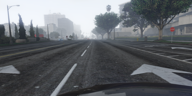
|
\bmvaHangBox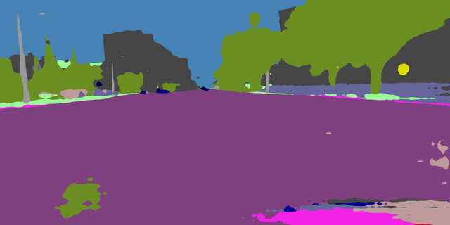
|
\bmvaHangBox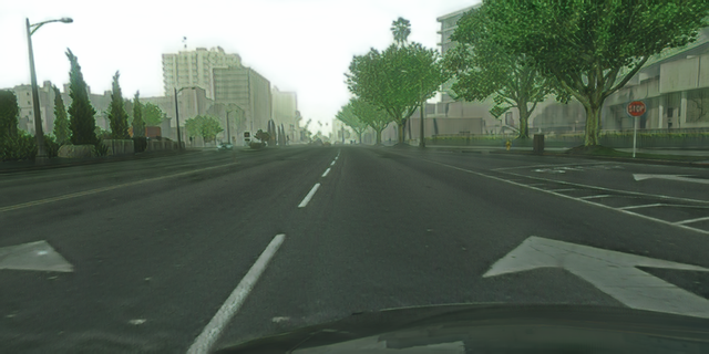
|
\bmvaHangBox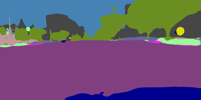
|
\bmvaHangBox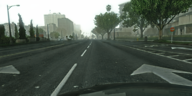
|
\bmvaHangBox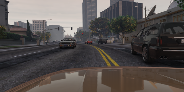
|
\bmvaHangBox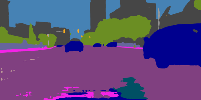
|
\bmvaHangBox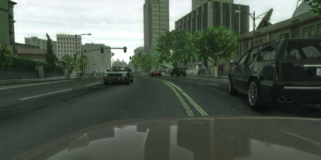
|
\bmvaHangBox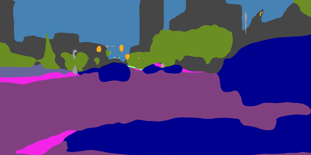
|
\bmvaHangBox
|
\bmvaHangBox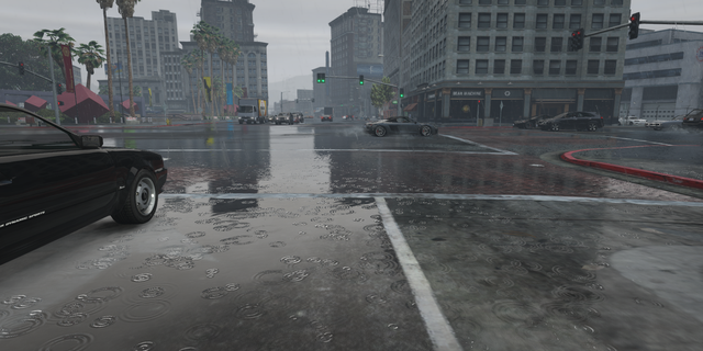
|
\bmvaHangBox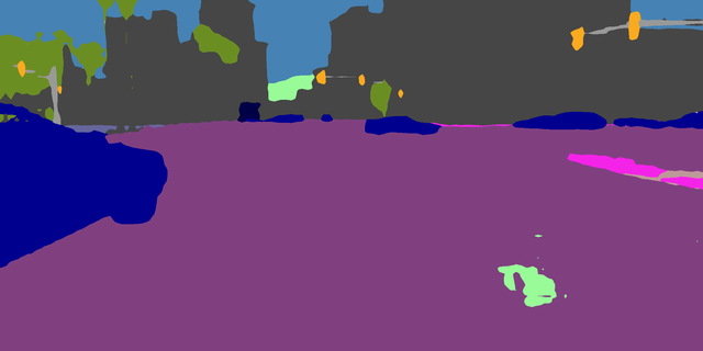
|
\bmvaHangBox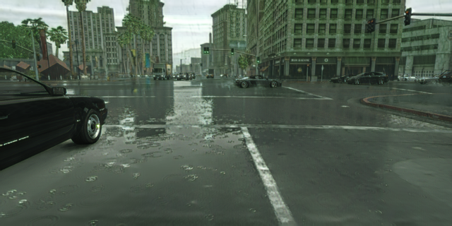
|
\bmvaHangBox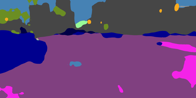
|
\bmvaHangBox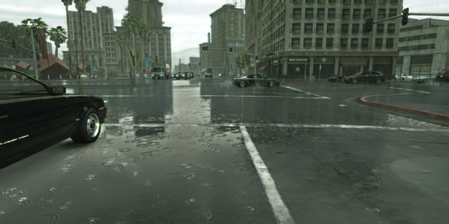
|
\bmvaHangBox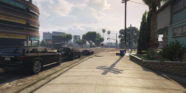
|
\bmvaHangBox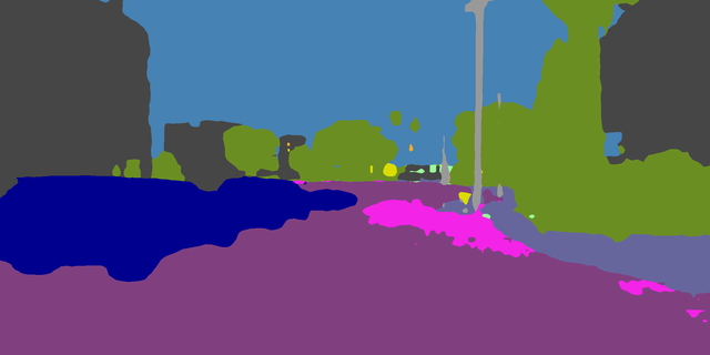
|
\bmvaHangBox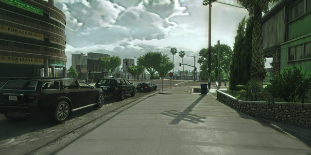
|
\bmvaHangBox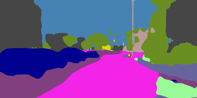
|
\bmvaHangBox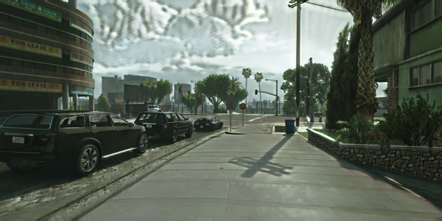
|
| GTA5 sample | GTA5 pred (D) | GTA5 CS (D) | GTA5 pred (F) | GTA5 CS (F) |
3 Method
Our objective is to train a deep neural network to perform semantic segmentation on a target (real) dataset . We assume we only have the target images without the target labels . In order to do this, we use synthetic data from a source (synthetic) dataset , where we have both the images and the labels .
This problem setting is UDA for semantic segmentation, which means that we want to reduce the domain shift caused by the difference in visual appearance of the two domains.
As depicted in Figure 2, we follow the recent work [Hoffman et al.(2018)Hoffman, Tzeng, Park, Zhu, Isola, Saenko, Efros, and Darrell, Chen et al.(2019)Chen, Lin, Yang, and Huang, Li et al.(2019)Li, Yuan, and Vasconcelos] and take advantage of both pixel-level and feature-level alignment to reduce the domain shift. We can see them as two separate subtasks, but we will also show how they actually need to cooperate to improve each other in the following sections.
3.1 Pixel-level alignment
 |
 |
 |
 |
 |
 |
 |
 |
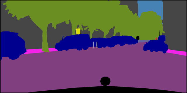
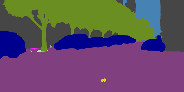
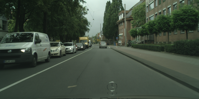
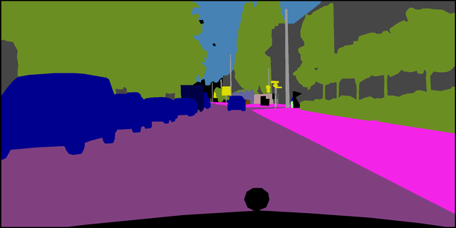
| Test sample | Ground truth | GTA5 CS w/ D | GTA5 CS w/ F |
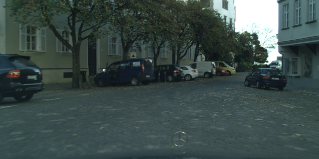
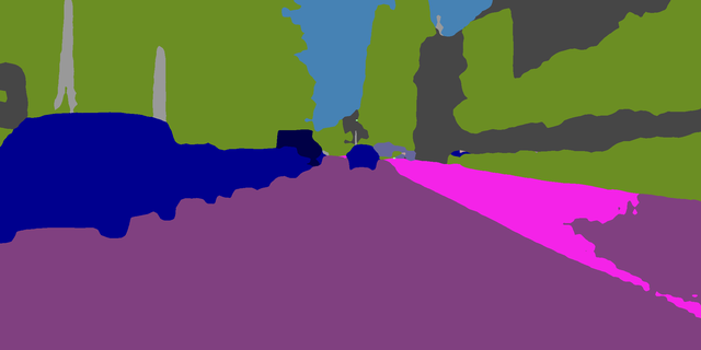
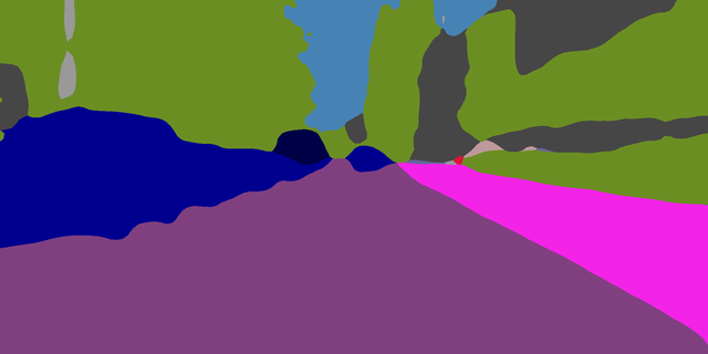
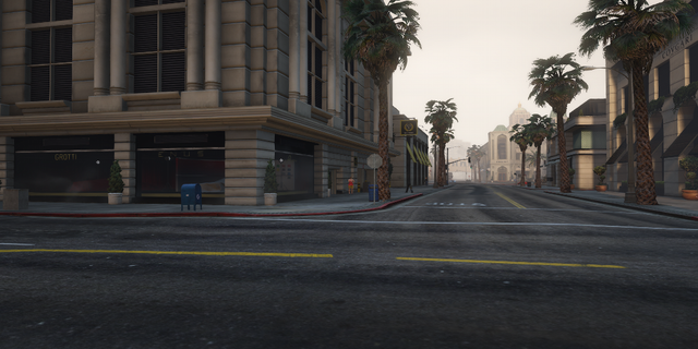
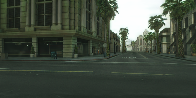
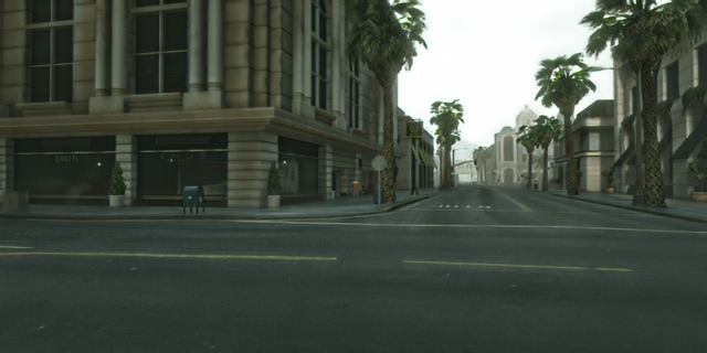
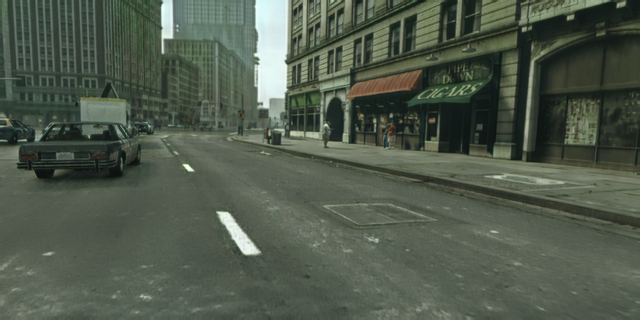
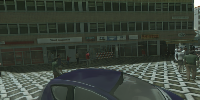
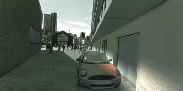
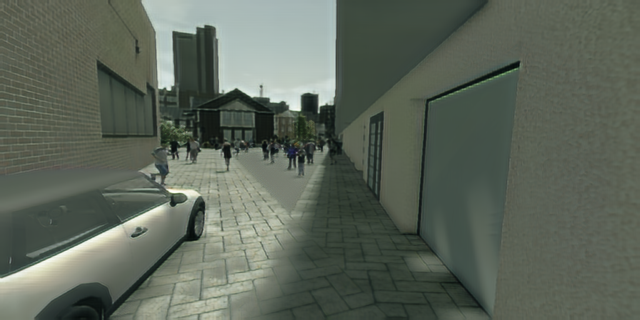
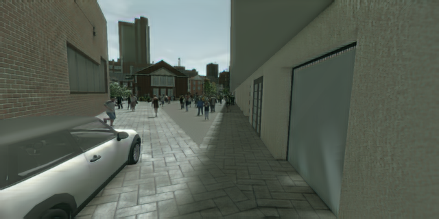
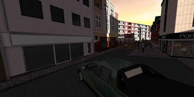
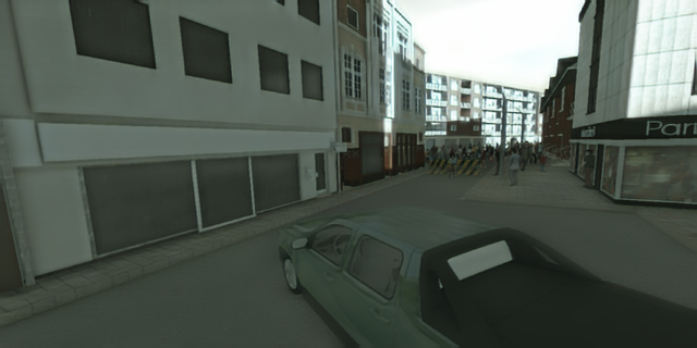
For pixel-level alignment, we make use of an image-to-image translation network , which learns through adversarial training to visually align to by generating . Some visual examples of the results of this pipeline are depicted in Figure 6. Inspired by [Liu et al.(2017)Liu, Breuel, and Kautz] [Huang et al.(2018)Huang, Liu, Belongie, and Kautz], we assume that and share a common latent space and design two coupled GANs to train the desired system.
The training objective for the image translation model is comprised of several loss functions computed as the sum of two components, one per domain. The final objective is then:
| (1) |
Image reconstruction
We have an encoder for each domain, and , coupled with a corresponding generator for each domain, and , to form two Autoencoders. The encoders extract the latent code , which is fed to the generators along with the semantic features predicted by . Therefore, a translated image is indicated as and the image reconstruction loss is:
| (2) |
Adversarial loss
By combining with and vice versa, we get the actual translation models and , which are trained in an adversarial fashion to trick the corresponding discriminators and :
| (3) | ||||
Cycle consistency
By combining with and viceversa we can now apply the cycle consistency loss to images and latent spaces:
| (4) | ||||
where refers to the latent space extracted by from and viceversa.
Symmetric cross-entropy
Finally, we impose that the segmentation predicted for the translated image has to be consistent with the one predicted for the original one through a symmetric cross-entropy loss, which is made of two contributions. For the case, the first contribution assumes that is the ground truth label and tries to align with it. The second contribution assumes that is the ground truth label and tries to align with it. The case is symmetrical to the first one.
| (5) | ||||
3.2 Semantically adaptive generator
Recent generator architectures [Huang et al.(2018)Huang, Liu, Belongie, and Kautz, Liu et al.(2019)Liu, Huang, Mallya, Karras, Aila, Lehtinen, and Kautz, Karras et al.(2019)Karras, Laine, and Aila] make use of AdaIN to remove the source style and inject the target one. However, we observe that the global denormalization performed by AdaIN might be suboptimal for the image translation task. This is why we redesigned our generator to adaptively denormalize each pixel based on its semantics.
We use to extract a segmentation map from the input image, where is the number of classes. When feeding it to the generator, we choose to represent this semantic guidance as the unnormalized output of . In the supplementary material we detail the reasons behind this choice and the other possibilities.
Given an input activation , is resized to and fed to the SPADE layer, which outputs . We then normalize by using Instance Normalization and use and to denormalize it:
| (6) |
3.3 Analysis
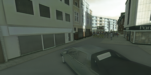
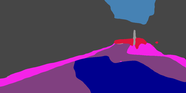
Pixel-level alignment has given a great boost to the research in UDA problems, but the gap with the performance achievable with full supervision is still huge. We believe that the image translation methods still need a lot of improvements and this is why we focused on redesigning the generator to include a semantic conditioning. Our claim is that adaptively denormalizing each pixel based on its class allows the translation model to produce results which are better for domain adaptation, since each region gets injected with features that are more consistent with its semantic. This connection strengthens the bridge with feature-level alignment (see Figure 1), which before our work was induced only by consistency losses.
3.4 Feature-level alignment
For feature-level alignment, we train on and by combining supervision on , self-supervision on and adversarial learning. The loss, in this case, is given by
| (7) |
We set , , for DeepLabV2, for FCN8s and use the same optimization hyperparameters of [Li et al.(2019)Li, Yuan, and Vasconcelos] to train both networks.
| GTA5 Cityscapes | |||||||||||||||||||||
| Method |
Arch. |
road |
sidewalk |
building |
wall |
fence |
pole |
light |
sign |
veget |
terrain |
sky |
person |
rider |
car |
truck |
bus |
train |
mbike |
bike |
mIoU |
| Cycada [Hoffman et al.(2018)Hoffman, Tzeng, Park, Zhu, Isola, Saenko, Efros, and Darrell] | D | 86.7 | 35.6 | 80.1 | 19.8 | 17.5 | 38.0 | 39.9 | 41.5 | 82.7 | 27.9 | 73.6 | 64.9 | 19 | 65.0 | 12.0 | 28.6 | 4.5 | 31.1 | 42.0 | 42.7 |
| AdaptSegNet [Tsai et al.(2018)Tsai, Hung, Schulter, Sohn, Yang, and Chandraker] | D | 86.5 | 25.9 | 79.8 | 22.1 | 20.0 | 23.6 | 33.1 | 21.8 | 81.8 | 25.9 | 75.9 | 57.3 | 26.2 | 76.3 | 29.8 | 32.1 | 7.2 | 29.5 | 32.5 | 41.4 |
| DCAN [Wu et al.(2018)Wu, Han, Lin, Gokhan Uzunbas, Goldstein, Nam Lim, and Davis] | D | 85.0 | 30.8 | 81.3 | 25.8 | 21.2 | 22.2 | 25.4 | 26.6 | 83.4 | 36.7 | 76.2 | 58.9 | 24.9 | 80.7 | 29.5 | 42.9 | 2.5 | 26.9 | 11.6 | 41.7 |
| CLAN [Luo et al.(2019)Luo, Zheng, Guan, Yu, and Yang] | D | 87.0 | 27.1 | 79.6 | 27.3 | 23.3 | 28.3 | 35.5 | 24.2 | 83.6 | 27.4 | 74.2 | 58.6 | 28.0 | 76.2 | 33.1 | 36.7 | 6.7 | 31.9 | 31.4 | 43.2 |
| BDL [Li et al.(2019)Li, Yuan, and Vasconcelos] | D | 91.0 | 44.7 | 84.2 | 34.6 | 27.6 | 30.2 | 36.0 | 36.0 | 85.0 | 43.6 | 83.0 | 58.6 | 31.6 | 83.3 | 35.3 | 49.7 | 3.3 | 28.8 | 35.6 | 48.5 |
| Ours | D | 91.2 | 43.3 | 85.2 | 38.6 | 25.9 | 34.7 | 41.3 | 41.0 | 85.5 | 46.0 | 86.5 | 61.7 | 33.8 | 85.5 | 34.4 | 48.7 | 0.0 | 36.1 | 37.8 | 50.4 |
| Curriculum [Zhang et al.(2017)Zhang, David, and Gong] | F | 74.9 | 22.0 | 71.7 | 6.0 | 11.9 | 8.4 | 16.3 | 11.1 | 75.7 | 13.3 | 66.5 | 38.0 | 9.3 | 55.2 | 18.8 | 18.9 | 0.0 | 16.8 | 16.6 | 28.9 |
| CBST [Zou et al.(2018)Zou, Yu, Vijaya Kumar, and Wang] | F | 66.7 | 26.8 | 73.7 | 14.8 | 9.5 | 28.3 | 25.9 | 10.1 | 75.5 | 15.7 | 51.6 | 47.2 | 6.2 | 71.9 | 3.7 | 2.2 | 5.4 | 18.9 | 32.4 | 30.9 |
| Cycada [Hoffman et al.(2018)Hoffman, Tzeng, Park, Zhu, Isola, Saenko, Efros, and Darrell] | F | 85.2 | 37.2 | 76.5 | 21.8 | 15.0 | 23.8 | 22.9 | 21.5 | 80.5 | 31.3 | 60.7 | 50.5 | 9.0 | 76.9 | 17.1 | 28.2 | 4.5 | 9.8 | 0.0 | 35.4 |
| DCAN [Wu et al.(2018)Wu, Han, Lin, Gokhan Uzunbas, Goldstein, Nam Lim, and Davis] | F | 82.3 | 26.7 | 77.4 | 23.7 | 20.5 | 20.4 | 30.3 | 15.9 | 80.9 | 25.4 | 69.5 | 52.6 | 11.1 | 79.6 | 24.9 | 21.2 | 1.3 | 17.0 | 6.7 | 36.2 |
| LSD [Sankaranarayanan et al.(2018)Sankaranarayanan, Balaji, Jain, Nam Lim, and Chellappa] | F | 88.0 | 30.5 | 78.6 | 25.2 | 23.5 | 16.7 | 23.5 | 11.6 | 78.7 | 27.2 | 71.9 | 51.3 | 19.5 | 80.4 | 19.8 | 18.3 | 0.9 | 20.8 | 18.4 | 37.1 |
| CLAN [Luo et al.(2019)Luo, Zheng, Guan, Yu, and Yang] | F | 88.0 | 30.6 | 79.2 | 23.4 | 20.5 | 26.1 | 23.0 | 14.8 | 81.6 | 34.5 | 72.0 | 45.8 | 7.9 | 80.5 | 26.6 | 29.9 | 0.0 | 10.7 | 0.0 | 36.6 |
| CrDoCo [Chen et al.(2019)Chen, Lin, Yang, and Huang] | F | 89.1 | 33.2 | 80.1 | 26.9 | 25.0 | 18.3 | 23.4 | 12.8 | 77.0 | 29.1 | 72.4 | 55.1 | 20.2 | 79.9 | 22.3 | 19.5 | 1.0 | 20.1 | 18.7 | 38.1 |
| BDL [Li et al.(2019)Li, Yuan, and Vasconcelos] | F | 89.2 | 40.9 | 81.2 | 29.1 | 19.2 | 14.2 | 29.0 | 19.6 | 83.7 | 35.9 | 80.7 | 54.7 | 23.3 | 82.7 | 25.8 | 28.0 | 2.3 | 25.7 | 19.9 | 41.3 |
| Ours | F | 91.1 | 46.4 | 82.9 | 33.2 | 27.9 | 20.6 | 29.0 | 28.2 | 84.5 | 40.9 | 82.3 | 52.4 | 24.4 | 81.2 | 21.8 | 44.8 | 31.5 | 26.5 | 33.7 | 46.5 |
Segmentation loss
The main supervision for the segmentation task is given by training the network on , where are images translated from the synthetic to the real domain. This is formulated as the common cross-entropy loss:
| (8) |
Self-supervised segmentation
Following [Li et al.(2019)Li, Yuan, and Vasconcelos], we also adopt self-supervision to improve the adaptation model. To this end, we compute and use as labels the high confidence predictions, creating :
| (9) |
where is the number of classes, is the index ignored and is the confidence threshold, which we use to filter the uncertain predictions. In our experiments we set .
This makes us able to compute a cross-entropy loss also on the target dataset:
| (10) |
Adversarial loss
Supervision on pixel-level aligned images and self-supervision on target images are not enough to learn a full model. This is why we also make use of adversarial training by feeding the semantic maps to a discriminator , which has to distinguish the maps predicted by for and , giving:
| (11) |
This loss enforces an output space alignment [Tsai et al.(2018)Tsai, Hung, Schulter, Sohn, Yang, and Chandraker], which means that has to learn how to predict semantic maps with distributions that are aligned regardless of the input domain.
4 Experiments
| SYNTHIA Cityscapes | ||||||||||||||||||
| Method |
Arch. |
road |
sidewalk |
building |
wall |
fence |
pole |
light |
sign |
veget |
sky |
person |
rider |
car |
bus |
mbike |
bike |
mIoU |
| AdaptSegNet [Tsai et al.(2018)Tsai, Hung, Schulter, Sohn, Yang, and Chandraker] | D | 79.2 | 37.2 | 78.8 | - | - | - | 9.9 | 10.5 | 78.2 | 80.5 | 53.5 | 19.6 | 67.0 | 29.5 | 21.6 | 31.3 | 45.9 |
| CLAN [Luo et al.(2019)Luo, Zheng, Guan, Yu, and Yang] | D | 81.3 | 37.0 | 80.1 | - | - | - | 16.1 | 13.7 | 78.2 | 81.5 | 53.4 | 21.2 | 73.0 | 32.9 | 22.6 | 30.7 | 47.8 |
| BDL [Li et al.(2019)Li, Yuan, and Vasconcelos] | D | 86.0 | 46.7 | 80.3 | - | - | - | 14.1 | 11.6 | 79.2 | 81.3 | 54.1 | 27.9 | 73.7 | 42.2 | 25.7 | 45.3 | 51.4 |
| Ours | D | 87.7 | 49.7 | 81.6 | - | - | - | 19.3 | 18.5 | 81.1 | 83.7 | 58.7 | 31.8 | 73.3 | 47.9 | 37.1 | 45.7 | 55.1 |
| FCNsITW [Hoffman et al.(2016)Hoffman, Wang, Yu, and Darrell] | F | 11.5 | 19.6 | 30.8 | 4.4 | 0.0 | 20.3 | 0.1 | 11.7 | 42.3 | 68.7 | 51.2 | 3.8 | 54.0 | 3.2 | 0.2 | 0.6 | 20.2 |
| Curriculum [Zhang et al.(2017)Zhang, David, and Gong] | F | 65.2 | 26.1 | 74.9 | 0.1 | 0.5 | 10.7 | 3.5 | 3.0 | 76.1 | 70.6 | 47.1 | 8.2 | 43.2 | 20.7 | 0.7 | 13.1 | 29.0 |
| CBST [Zou et al.(2018)Zou, Yu, Vijaya Kumar, and Wang] | F | 69.6 | 28.7 | 69.5 | 12.1 | 0.1 | 25.4 | 11.9 | 13.6 | 82.0 | 81.9 | 49.1 | 14.5 | 66.0 | 6.6 | 3.7 | 32.4 | 35.4 |
| DCAN [Wu et al.(2018)Wu, Han, Lin, Gokhan Uzunbas, Goldstein, Nam Lim, and Davis] | F | 79.9 | 30.4 | 70.8 | 1.6 | 0.6 | 22.3 | 6.7 | 23.0 | 76.9 | 73.9 | 41.9 | 16.7 | 61.7 | 11.5 | 10.3 | 38.6 | 35.4 |
| CLAN [Luo et al.(2019)Luo, Zheng, Guan, Yu, and Yang] | F | 80.4 | 30.7 | 74.7 | - | - | - | 1.4 | 8.0 | 77.1 | 79.0 | 46.5 | 8.9 | 73.8 | 18.2 | 2.2 | 9.9 | 39.3 |
| CrDoCo [Chen et al.(2019)Chen, Lin, Yang, and Huang] | F | 84.9 | 32.8 | 80.1 | 4.3 | 0.4 | 29.4 | 14.2 | 21.0 | 79.2 | 78.3 | 50.2 | 15.9 | 69.8 | 23.4 | 11.0 | 15.6 | 38.2 |
| BDL [Li et al.(2019)Li, Yuan, and Vasconcelos] | F | 72.0 | 30.3 | 74.5 | 0.1 | 0.3 | 24.6 | 10.2 | 25.2 | 80.5 | 80.0 | 54.7 | 23.2 | 72.7 | 24.0 | 7.5 | 44.9 | 39.0 |
| Ours | F | 79.1 | 34.0 | 78.3 | 0.3 | 0.6 | 26.7 | 15.9 | 29.5 | 81.0 | 81.1 | 55.5 | 21.9 | 77.2 | 23.5 | 11.8 | 47.5 | 41.5 |
We present our experimental results for the synthetic to real adaptation using two dataset settings: GTA5 [Richter et al.(2016)Richter, Vineet, Roth, and Koltun] to Cityscapes [Cordts et al.(2016)Cordts, Omran, Ramos, Rehfeld, Enzweiler, Benenson, Franke, Roth, and Schiele] and SYNTHIA [Ros et al.(2016)Ros, Sellart, Materzynska, Vazquez, and Lopez] to Cityscapes. We evaluate the mean intersection-over-union (IoU) on the Cityscapes validation set and show how our method outperforms the current state-of-the-art by adopting the same segmentation models. Finally, we conduct an ablation study to highlight the value of our contributions.
Segmentation network
We choose to adapt two segmentation networks: DeepLabV2 [Chen et al.(2017a)Chen, Papandreou, Kokkinos, Murphy, and Yuille] with ResNet101 [He et al.(2016)He, Zhang, Ren, and Sun] and FCN8s [Long et al.(2015a)Long, Shelhamer, and Darrell] with VGG16 [Simonyan and Zisserman(2014)]. Both networks are trained on images downsampled to 1024x512 with batch size 1.
We initialize the segmentation networks from [Li et al.(2019)Li, Yuan, and Vasconcelos] to speed up the training process. In order to show the independence from this initialization, we also conduct one experiment where we train DeepLabV2 from scratch for the GTACityscapes task, and we find this to be in line with the results that we get by initializing it with [Li et al.(2019)Li, Yuan, and Vasconcelos].
Translation network
For the translation part, we describe the architecture of the encoders, generators and discriminators.
The encoder is made by few downsampling blocks, followed by residual blocks for further processing of the latent code and they all use IN [Ulyanov et al.(2016b)Ulyanov, Vedaldi, and Lempitsky]. Symmetrically, the generators take in the latent code and process it with residual blocks, where IN and SPADE are combined to normalize the feature maps. These are followed by upsampling blocks with Layer Normalization [Ba et al.(2016)Ba, Kiros, and Hinton]. We found LN to better preserve the style in the generated activations.
In each domain we have discriminators for multiple scales [Wang et al.(2018)Wang, Liu, Zhu, Tao, Kautz, and Catanzaro], each being a Patch Discriminator [Isola et al.(2017)Isola, Zhu, Zhou, and Efros, Li and Wand(2016)]. The GAN [Goodfellow et al.(2014)Goodfellow, Pouget-Abadie, Mirza, Xu, Warde-Farley, Ozair, Courville, and Bengio] objective we choose is the one proposed in LSGAN [Mao et al.(2017)Mao, Li, Xie, Lau, Wang, and Paul Smolley]. We apply Spectral Normalization [Miyato et al.(2018)Miyato, Kataoka, Koyama, and Yoshida] to all the models described here.
When training the translation model we resize the input images to 1024x512 and take 512x512 random crops out of them. We use Adam [Kingma and Ba(2014)] as optimizer with and . We apply TTUR [Heusel et al.(2017)Heusel, Ramsauer, Unterthiner, Nessler, and Hochreiter] and set the initial learning rate to be . The learning rate is scheduled to decay to after 1000000 iterations with a ’poly’ scheduling where the power is . The batch size is 1 for all the experiments. The loss weights are set to , , , , .
Bidirectional learning
Pixel-level and feature-level alignment are not performed in an end-to-end fashion. Besides being highly expensive in terms of memory requirements, we found this approach to be very unstable and it did not lead to good results.
We adopt a policy similar to [Li et al.(2019)Li, Yuan, and Vasconcelos] and iteratively recreate when stops improving on the target dataset. Before each training of the segmentation network, we also generate new pseudo-labels . We found this procedure to significantly improve the final mIoU compared to a single iteration of pixel-level and feature-level alignment.
4.1 Comparison with State of the Art
GTA5 to Cityscapes
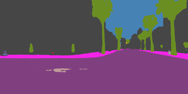
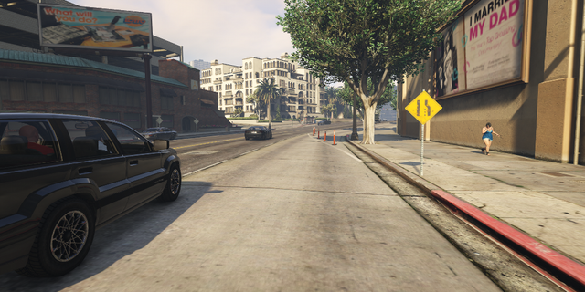
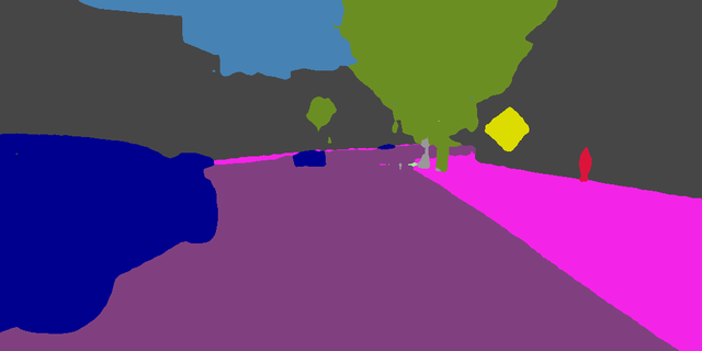
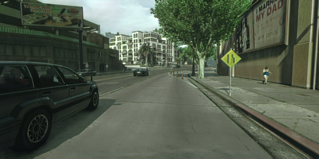
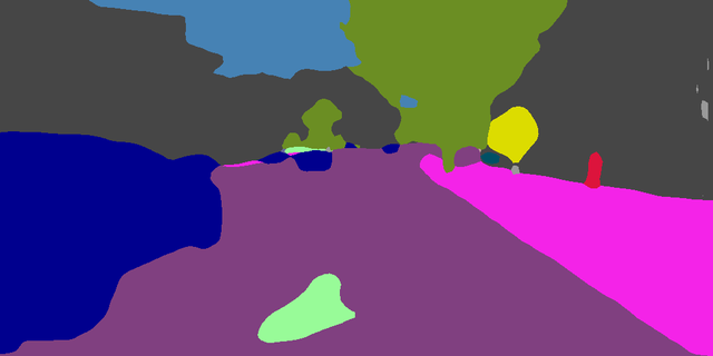
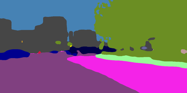
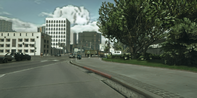
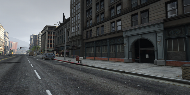
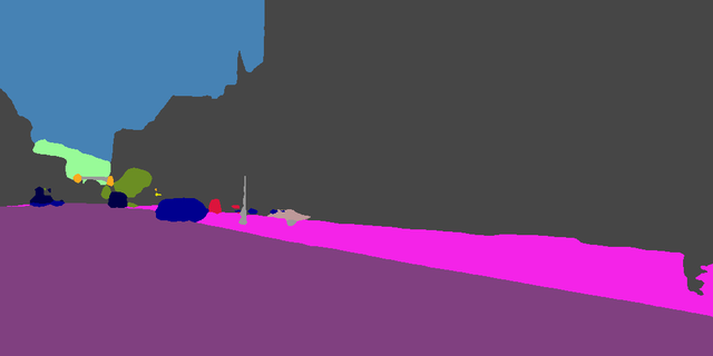
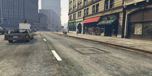
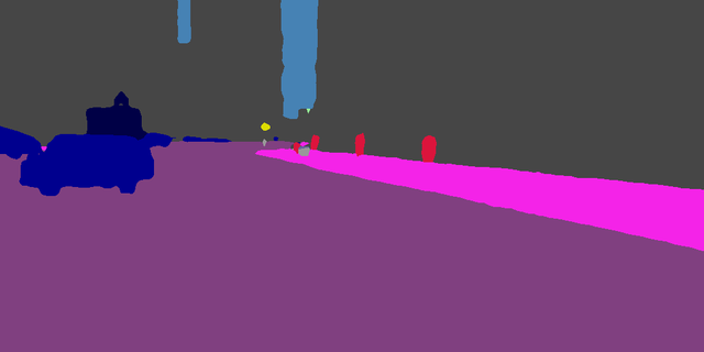
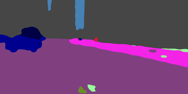
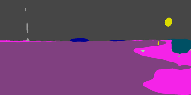
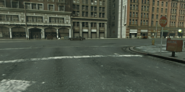
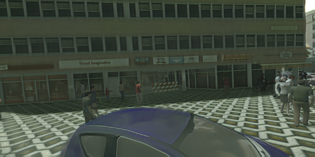
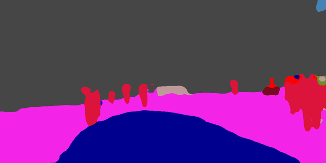
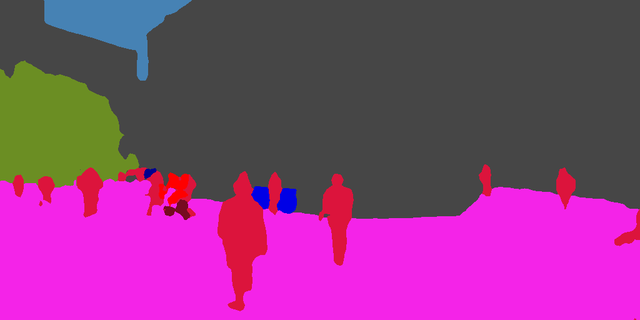
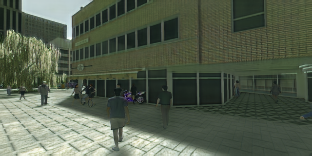
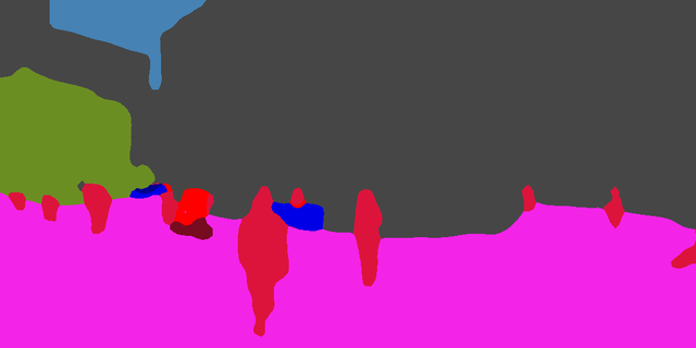
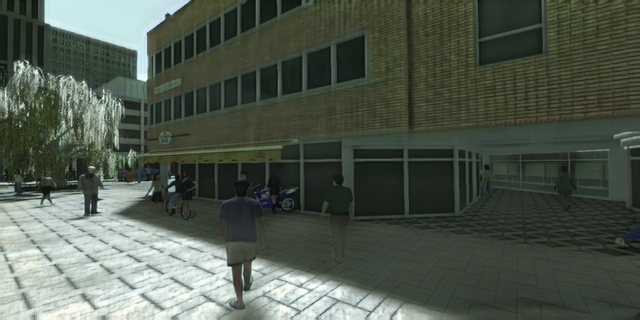
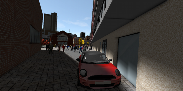
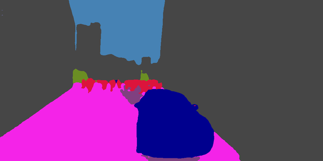
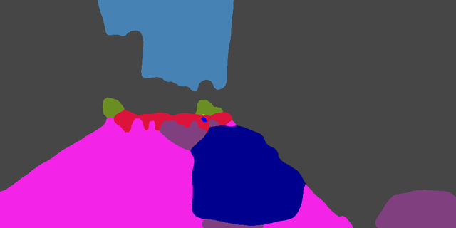
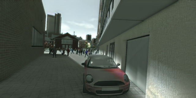
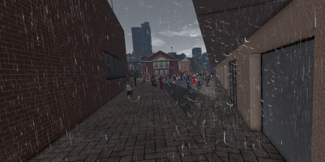
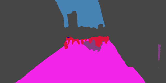
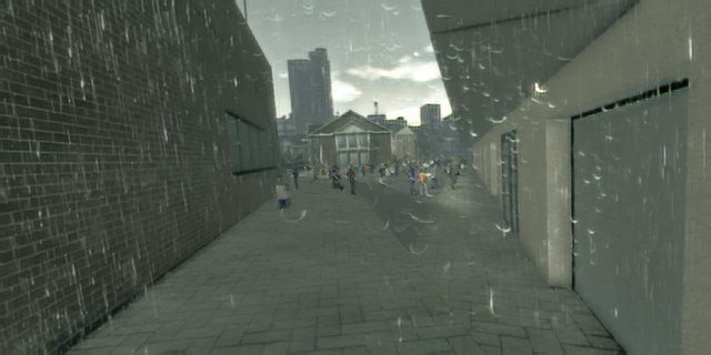
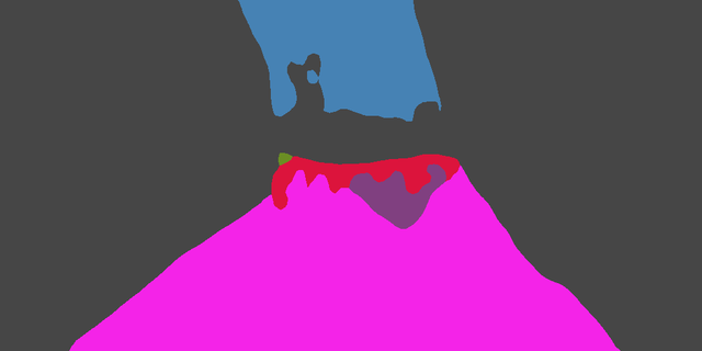
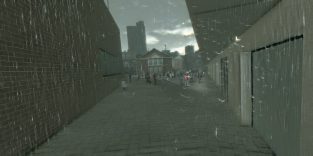
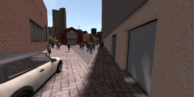
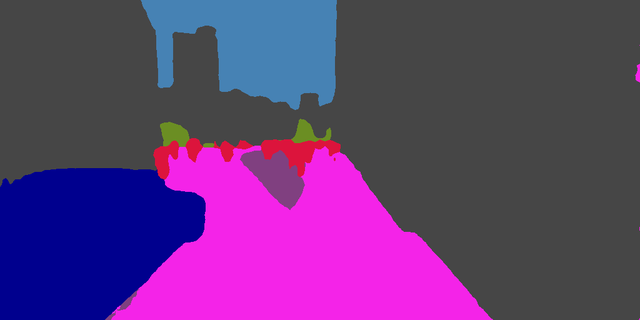
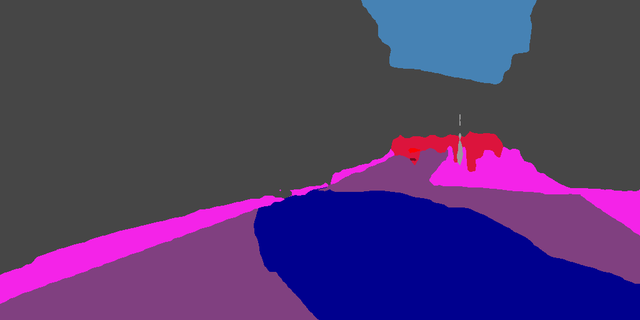
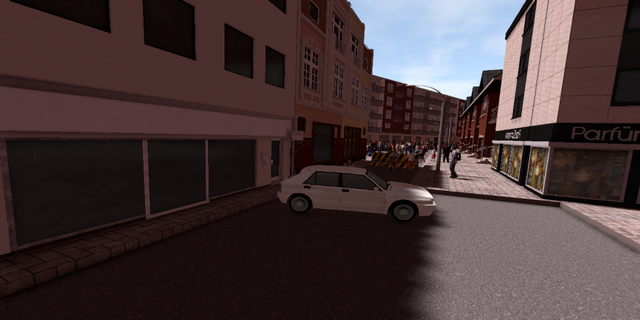
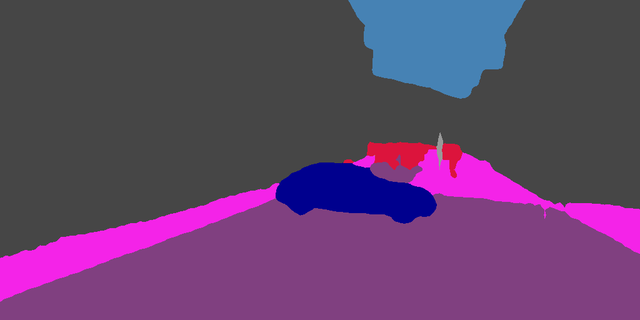
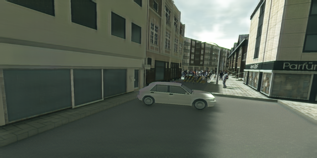
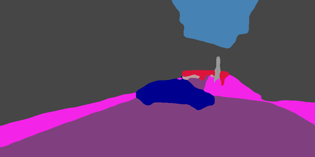
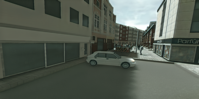
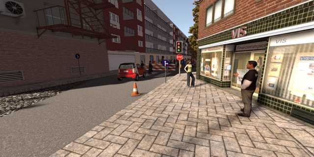
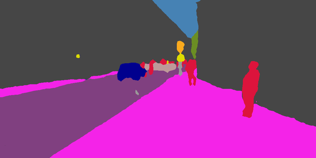
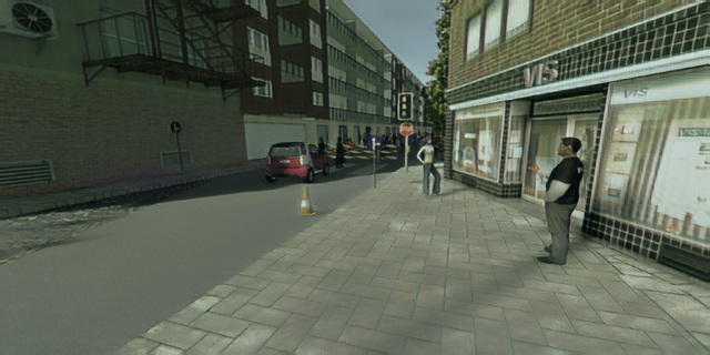
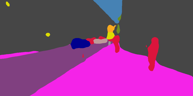
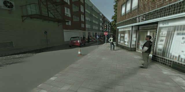
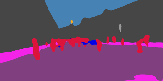
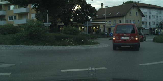
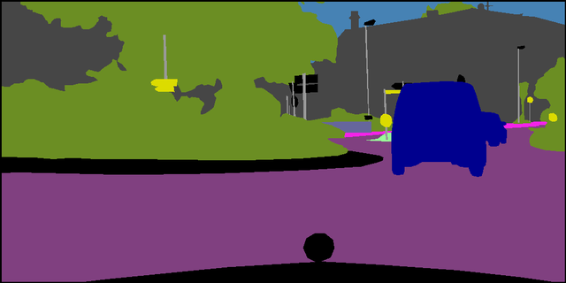
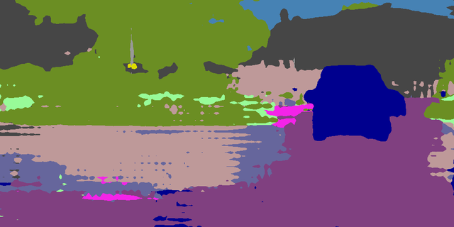
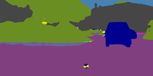
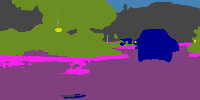
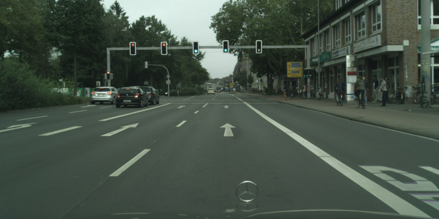
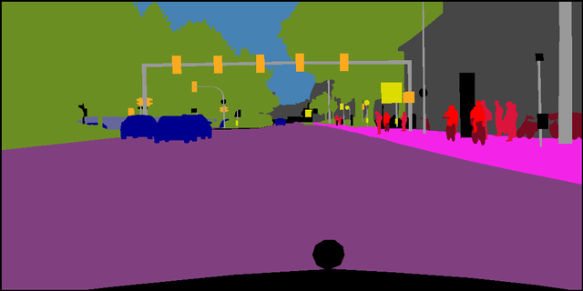
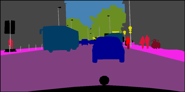
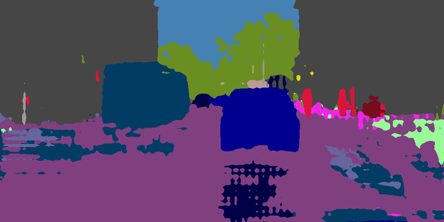
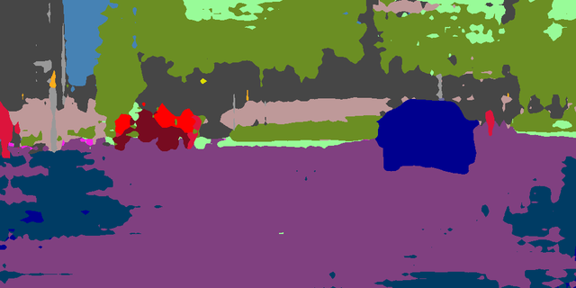
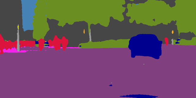
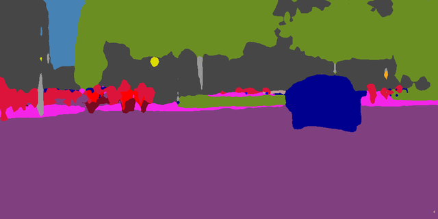
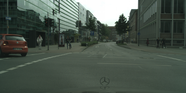
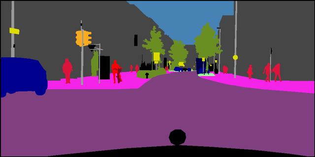
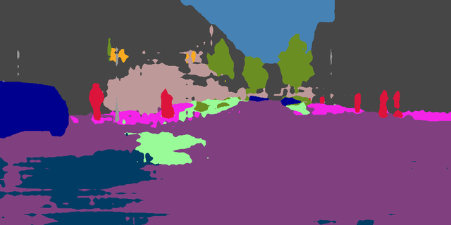
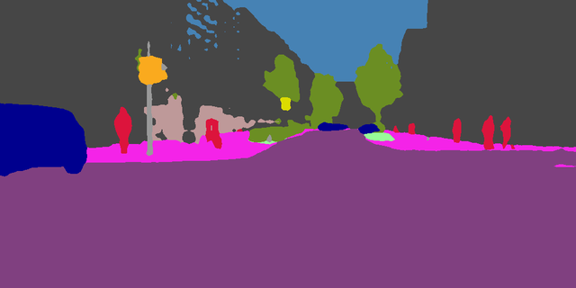
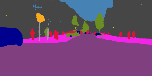
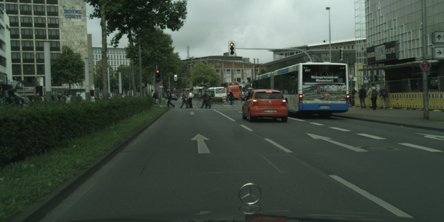
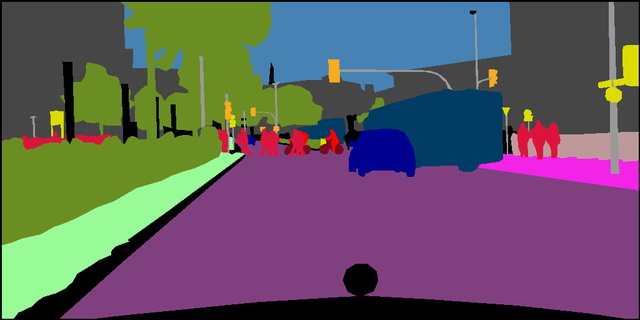
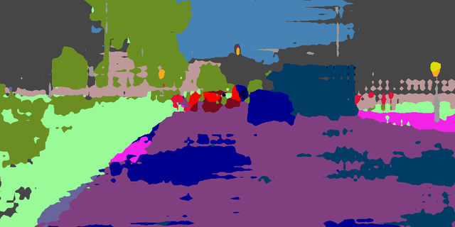
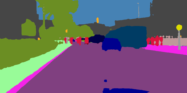
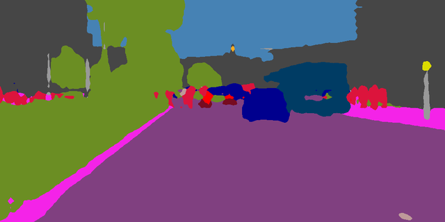
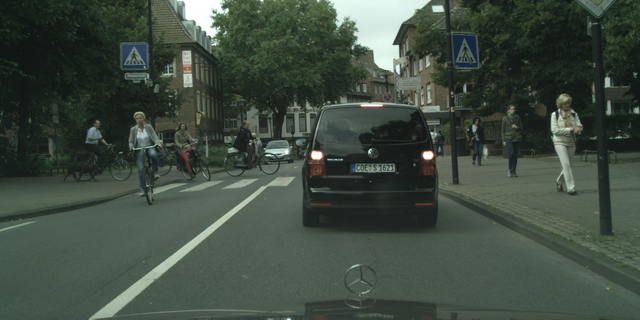
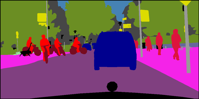
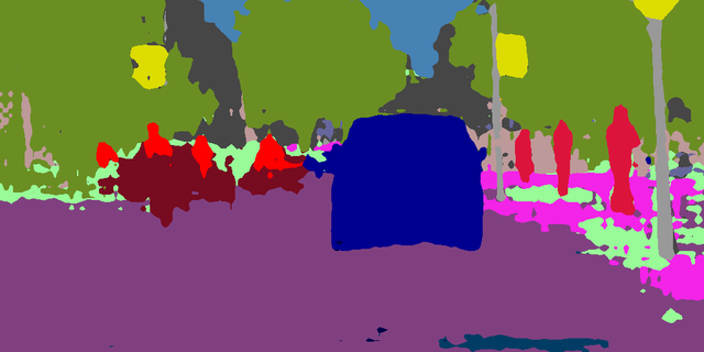
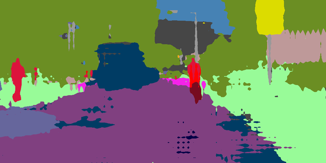
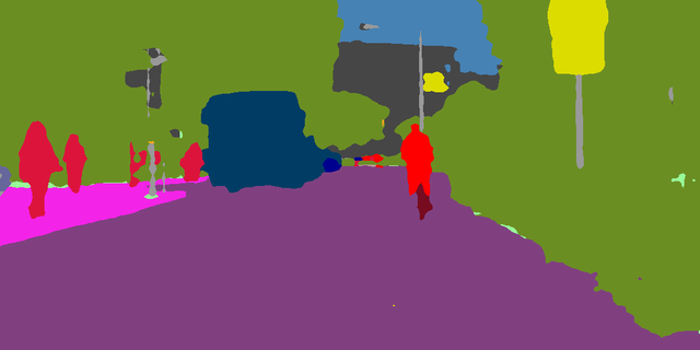
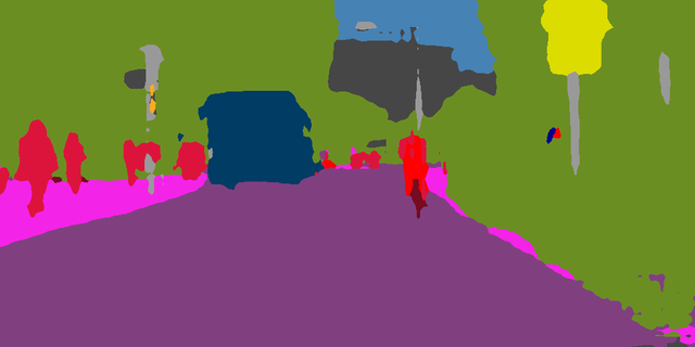
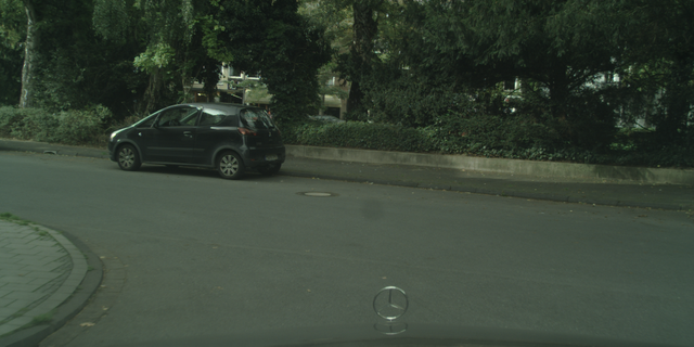
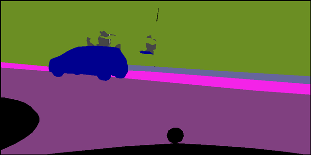
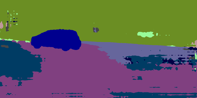
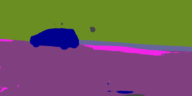
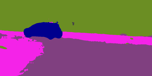
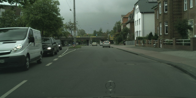
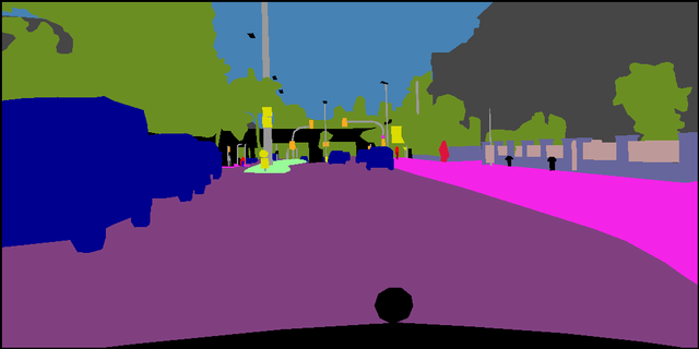
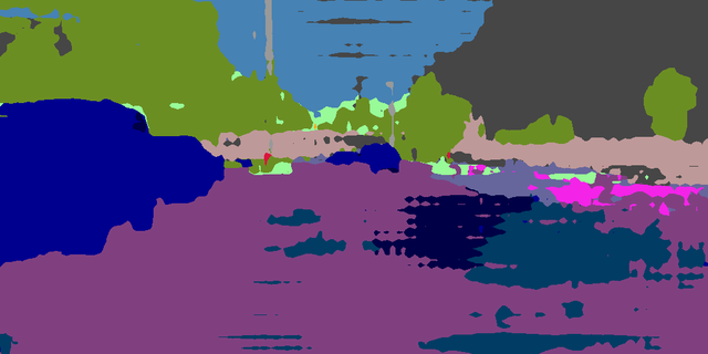
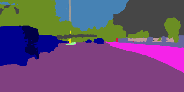
For the GTA5 [Richter et al.(2016)Richter, Vineet, Roth, and Koltun] to Cityscapes [Cordts et al.(2016)Cordts, Omran, Ramos, Rehfeld, Enzweiler, Benenson, Franke, Roth, and Schiele] task, we evaluate on all the 19 classes used in the Cityscapes benchmark since the datasets are fully compatible. Some visual results for this setting are presented in Figure 4. In this case, the upper bounds in terms of mIoU are 65.1 for DeepLabV2 [Chen et al.(2017a)Chen, Papandreou, Kokkinos, Murphy, and Yuille] and 60.3 for FCN8s [Long et al.(2015a)Long, Shelhamer, and Darrell], which are the results achievable by training with the target labels. In Table 1 we compare our results with the related work. In terms of mIoU, we get respectively +1.9% and +4.2% over the state-of-the-art with the two networks.
SYNTHIA to Cityscapes
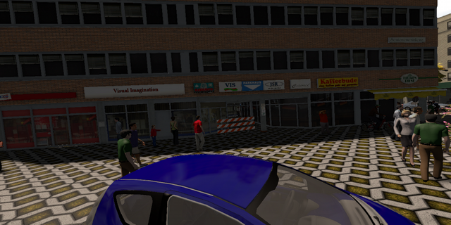
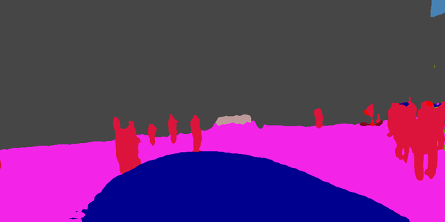
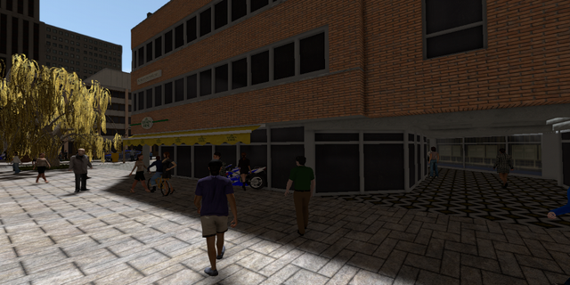
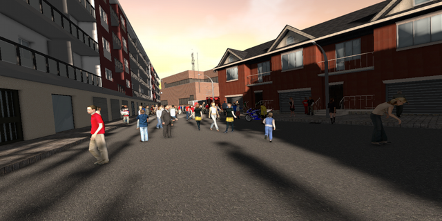
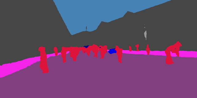
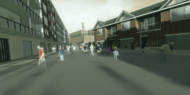
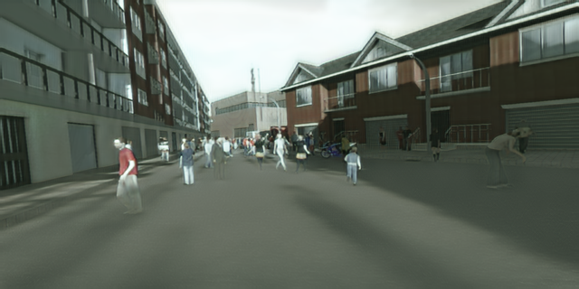
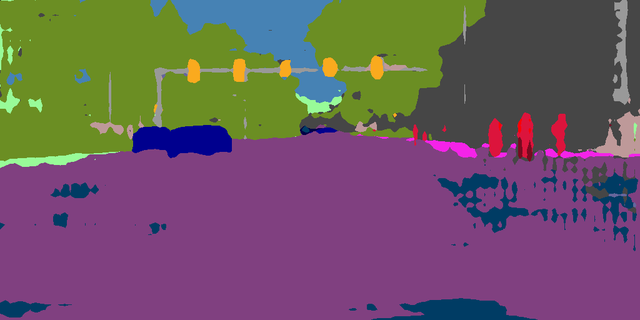
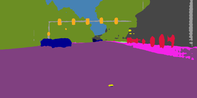
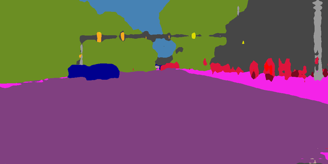
SYNTHIA [Ros et al.(2016)Ros, Sellart, Materzynska, Vazquez, and Lopez] has been adopted in the past by the other works for its overlapping with 16 of the Cityscapes classes. For the SYNTHIA to Cityscapes task we compare our results with the state-of-the-art in Table 2 and present some visual results in the supplementary material. For a fair comparison, the results of the DeepLabV2 architecture are limited to the 13 classes adopted by the other works [Tsai et al.(2018)Tsai, Hung, Schulter, Sohn, Yang, and Chandraker, Luo et al.(2019)Luo, Zheng, Guan, Yu, and Yang, Li et al.(2019)Li, Yuan, and Vasconcelos]. The upper bounds in terms of mIoU are 71.7 for DeepLabV2 and 59.5 for FCN8s. In the case of DeepLabV2 we surpass the current state-of-the-art in mIoU by +3.7%. For FCN8s, instead, we get +2.5% on the mIoU.
4.2 Ablation study
| SPADE | mIoU | Gain | Gap to UB | |
| 49.2 | 15.6 | 15.9 | ||
| ✓ | 49.5 | 15.9 | 15.6 | |
| ✓ | 49.5 | 15.9 | 15.6 | |
| ✓ | ✓ | 50.4 | 16.8 | 14.7 |
In order to weight our contribution, we perform an ablation study of the proposed method (see Table 3). For each experiment, we report 3 values: the mIoU; the gain wrt the lower bound, which is a naive training on the source dataset; the remaining gap wrt the upper bound, which is the result for training with target labels (called oracle prediction).
The experiments are conducted with DeepLabV2 [Chen et al.(2017a)Chen, Papandreou, Kokkinos, Murphy, and Yuille] for the GTA5 [Richter et al.(2016)Richter, Vineet, Roth, and Koltun] to Cityscapes [Cordts et al.(2016)Cordts, Omran, Ramos, Rehfeld, Enzweiler, Benenson, Franke, Roth, and Schiele] task, for which the lower bound is 33.6 and the upper bound is 65.1.
We first show the baseline results that we get by using the generator with no Symmetric Cross-Entropy and no semantic guidance. In this setting, the residual blocks of the generator use IN [Ulyanov et al.(2016b)Ulyanov, Vedaldi, and Lempitsky] layers and the image-to-image translation is completely unrelated to the semantic segmentation. Secondly, we add the semantic guidance with the SPADE [Park et al.(2019)Park, Liu, Wang, and Zhu] layer. This setting can still benefit from the semantic guidance in the translation, but loses the ability to enforce the cross-domain consistency for the segmentation task. Then we swap back the SPADE layer with IN and enable . This setting resembles the one used in [Chen et al.(2019)Chen, Lin, Yang, and Huang], where the architecture of CycleGAN [Zhu et al.(2017)Zhu, Park, Isola, and Efros] is replaced by ours. Finally, we show that the best results are achieved by the combination of the two elements, which completely bridges the translation and segmentation tasks and is the final setting of our work.
We can see that when we remove SPADE or the mIoU drops, suggesting that they both have an important contribution to get the best result.
4.3 Generated image quality
We also report the quality of the images generated by our image-to-image translation model. In Table 4 we report the Inception Score (IS) [Salimans et al.(2016)Salimans, Goodfellow, Zaremba, Cheung, Radford, and Chen] of the images and the Fréchet Inception Distance (FID) [Heusel et al.(2017)Heusel, Ramsauer, Unterthiner, Nessler, and Hochreiter] with the Cityscapes training set. Although the IS of the produced images is low in every setting, the FID results indicate that the semantic guidance induced by DeepLabV2 is the one that best visually aligns the synthetic domain to Cityscapes. The images translated from SYNTHIA, however, have a much greater distance from Cityscapes than the ones translated from GTA5, regardless of the network used as semantic guidance. We note that this is possibly due to the bigger initial gap in visual appearance between the two domains, since the FID between the original SYNTHIA and Cityscapes is 156.92, while the FID between the original GTA5 and Cityscapes is only 62.42.
| Setting | Network | IS | FID |
| GTA5 Cityscapes | DeepLabV2 | 4.9 | 27.9 |
| GTA5 Cityscapes | FCN8s | 4.8 | 40.3 |
| SYNTHIA Cityscapes | DeepLabV2 | 5.0 | 100.8 |
| SYNTHIA Cityscapes | FCN8s | 4.9 | 113.7 |
References
- [Ba et al.(2016)Ba, Kiros, and Hinton] Jimmy Lei Ba, Jamie Ryan Kiros, and Geoffrey E Hinton. Layer normalization. arXiv preprint arXiv:1607.06450, 2016.
- [Chen et al.(2017a)Chen, Papandreou, Kokkinos, Murphy, and Yuille] Liang-Chieh Chen, George Papandreou, Iasonas Kokkinos, Kevin Murphy, and Alan L Yuille. Deeplab: Semantic image segmentation with deep convolutional nets, atrous convolution, and fully connected crfs. IEEE transactions on pattern analysis and machine intelligence, 40(4):834–848, 2017a.
- [Chen et al.(2018)Chen, Liu, Wang, Wassell, and Chetty] Qingchao Chen, Yang Liu, Zhaowen Wang, Ian Wassell, and Kevin Chetty. Re-weighted adversarial adaptation network for unsupervised domain adaptation. In Proceedings of the IEEE Conference on Computer Vision and Pattern Recognition, pages 7976–7985, 2018.
- [Chen et al.(2017b)Chen, Chen, Chen, Tsai, Frank Wang, and Sun] Yi-Hsin Chen, Wei-Yu Chen, Yu-Ting Chen, Bo-Cheng Tsai, Yu-Chiang Frank Wang, and Min Sun. No more discrimination: Cross city adaptation of road scene segmenters. In Proceedings of the IEEE International Conference on Computer Vision, pages 1992–2001, 2017b.
- [Chen et al.(2019)Chen, Lin, Yang, and Huang] Yun-Chun Chen, Yen-Yu Lin, Ming-Hsuan Yang, and Jia-Bin Huang. Crdoco: Pixel-level domain transfer with cross-domain consistency. In Proceedings of the IEEE Conference on Computer Vision and Pattern Recognition, pages 1791–1800, 2019.
- [Cordts et al.(2016)Cordts, Omran, Ramos, Rehfeld, Enzweiler, Benenson, Franke, Roth, and Schiele] Marius Cordts, Mohamed Omran, Sebastian Ramos, Timo Rehfeld, Markus Enzweiler, Rodrigo Benenson, Uwe Franke, Stefan Roth, and Bernt Schiele. The cityscapes dataset for semantic urban scene understanding. In Proceedings of the IEEE conference on computer vision and pattern recognition, pages 3213–3223, 2016.
- [Diederik et al.(2014)Diederik, Welling, et al.] P Kingma Diederik, Max Welling, et al. Auto-encoding variational bayes. In Proceedings of the International Conference on Learning Representations (ICLR), 2014.
- [Dundar et al.(2018)Dundar, Liu, Wang, Zedlewski, and Kautz] Aysegul Dundar, Ming-Yu Liu, Ting-Chun Wang, John Zedlewski, and Jan Kautz. Domain stylization: A strong, simple baseline for synthetic to real image domain adaptation. arXiv preprint arXiv:1807.09384, 2018.
- [Ganin and Lempitsky(2015)] Yaroslav Ganin and Victor Lempitsky. Unsupervised domain adaptation by backpropagation. In Proceedings of the 32nd International Conference on International Conference on Machine Learning-Volume 37, pages 1180–1189. JMLR. org, 2015.
- [Ganin et al.(2016)Ganin, Ustinova, Ajakan, Germain, Larochelle, Laviolette, Marchand, and Lempitsky] Yaroslav Ganin, Evgeniya Ustinova, Hana Ajakan, Pascal Germain, Hugo Larochelle, François Laviolette, Mario Marchand, and Victor Lempitsky. Domain-adversarial training of neural networks. The Journal of Machine Learning Research, 17(1):2096–2030, 2016.
- [Geng et al.(2011)Geng, Tao, and Xu] Bo Geng, Dacheng Tao, and Chao Xu. Daml: Domain adaptation metric learning. IEEE Transactions on Image Processing, 20(10):2980–2989, 2011.
- [Goodfellow et al.(2014)Goodfellow, Pouget-Abadie, Mirza, Xu, Warde-Farley, Ozair, Courville, and Bengio] Ian Goodfellow, Jean Pouget-Abadie, Mehdi Mirza, Bing Xu, David Warde-Farley, Sherjil Ozair, Aaron Courville, and Yoshua Bengio. Generative adversarial nets. In Advances in neural information processing systems, pages 2672–2680, 2014.
- [He et al.(2016)He, Zhang, Ren, and Sun] Kaiming He, Xiangyu Zhang, Shaoqing Ren, and Jian Sun. Deep residual learning for image recognition. In Proceedings of the IEEE conference on computer vision and pattern recognition, pages 770–778, 2016.
- [Heusel et al.(2017)Heusel, Ramsauer, Unterthiner, Nessler, and Hochreiter] Martin Heusel, Hubert Ramsauer, Thomas Unterthiner, Bernhard Nessler, and Sepp Hochreiter. Gans trained by a two time-scale update rule converge to a local nash equilibrium. In Advances in Neural Information Processing Systems, pages 6626–6637, 2017.
- [Hoffman et al.(2016)Hoffman, Wang, Yu, and Darrell] Judy Hoffman, Dequan Wang, Fisher Yu, and Trevor Darrell. Fcns in the wild: Pixel-level adversarial and constraint-based adaptation. arXiv preprint arXiv:1612.02649, 2016.
- [Hoffman et al.(2018)Hoffman, Tzeng, Park, Zhu, Isola, Saenko, Efros, and Darrell] Judy Hoffman, Eric Tzeng, Taesung Park, Jun-Yan Zhu, Phillip Isola, Kate Saenko, Alexei Efros, and Trevor Darrell. Cycada: Cycle-consistent adversarial domain adaptation. In Proceedings of the 35th International Conference on Machine Learning, 2018.
- [Huang and Belongie(2017)] Xun Huang and Serge Belongie. Arbitrary style transfer in real-time with adaptive instance normalization. In Proceedings of the IEEE International Conference on Computer Vision, pages 1501–1510, 2017.
- [Huang et al.(2018)Huang, Liu, Belongie, and Kautz] Xun Huang, Ming-Yu Liu, Serge Belongie, and Jan Kautz. Multimodal unsupervised image-to-image translation. In Proceedings of the European Conference on Computer Vision (ECCV), pages 172–189, 2018.
- [Ioffe and Szegedy(2015)] Sergey Ioffe and Christian Szegedy. Batch normalization: Accelerating deep network training by reducing internal covariate shift. In International Conference on Machine Learning, pages 448–456, 2015.
- [Isola et al.(2017)Isola, Zhu, Zhou, and Efros] Phillip Isola, Jun-Yan Zhu, Tinghui Zhou, and Alexei A Efros. Image-to-image translation with conditional adversarial networks. In Proceedings of the IEEE conference on computer vision and pattern recognition, pages 1125–1134, 2017.
- [Karras et al.(2019)Karras, Laine, and Aila] Tero Karras, Samuli Laine, and Timo Aila. A style-based generator architecture for generative adversarial networks. In Proceedings of the IEEE Conference on Computer Vision and Pattern Recognition, pages 4401–4410, 2019.
- [Kingma and Ba(2014)] Diederik P Kingma and Jimmy Ba. Adam: A method for stochastic optimization. arXiv preprint arXiv:1412.6980, 2014.
- [Li and Wand(2016)] Chuan Li and Michael Wand. Precomputed real-time texture synthesis with markovian generative adversarial networks. In European Conference on Computer Vision, pages 702–716. Springer, 2016.
- [Li et al.(2019)Li, Yuan, and Vasconcelos] Yunsheng Li, Lu Yuan, and Nuno Vasconcelos. Bidirectional learning for domain adaptation of semantic segmentation. In Proceedings of the IEEE Conference on Computer Vision and Pattern Recognition, pages 6936–6945, 2019.
- [Liu and Tuzel(2016)] Ming-Yu Liu and Oncel Tuzel. Coupled generative adversarial networks. In Advances in neural information processing systems, pages 469–477, 2016.
- [Liu et al.(2017)Liu, Breuel, and Kautz] Ming-Yu Liu, Thomas Breuel, and Jan Kautz. Unsupervised image-to-image translation networks. In Advances in neural information processing systems, pages 700–708, 2017.
- [Liu et al.(2019)Liu, Huang, Mallya, Karras, Aila, Lehtinen, and Kautz] Ming-Yu Liu, Xun Huang, Arun Mallya, Tero Karras, Timo Aila, Jaakko Lehtinen, and Jan Kautz. Few-shot unsupervised image-to-image translation. In IEEE International Conference on Computer Vision (ICCV), 2019.
- [Long et al.(2015a)Long, Shelhamer, and Darrell] Jonathan Long, Evan Shelhamer, and Trevor Darrell. Fully convolutional networks for semantic segmentation. In Proceedings of the IEEE conference on computer vision and pattern recognition, pages 3431–3440, 2015a.
- [Long et al.(2015b)Long, Cao, Wang, and Jordan] Mingsheng Long, Yue Cao, Jianmin Wang, and Michael I Jordan. Learning transferable features with deep adaptation networks. In Proceedings of the 32nd International Conference on International Conference on Machine Learning-Volume 37, pages 97–105. JMLR. org, 2015b.
- [Long et al.(2016)Long, Zhu, Wang, and Jordan] Mingsheng Long, Han Zhu, Jianmin Wang, and Michael I Jordan. Unsupervised domain adaptation with residual transfer networks. In Advances in Neural Information Processing Systems, pages 136–144, 2016.
- [Luo et al.(2019)Luo, Zheng, Guan, Yu, and Yang] Yawei Luo, Liang Zheng, Tao Guan, Junqing Yu, and Yi Yang. Taking a closer look at domain shift: Category-level adversaries for semantics consistent domain adaptation. In Proceedings of the IEEE Conference on Computer Vision and Pattern Recognition, pages 2507–2516, 2019.
- [Mao et al.(2017)Mao, Li, Xie, Lau, Wang, and Paul Smolley] Xudong Mao, Qing Li, Haoran Xie, Raymond YK Lau, Zhen Wang, and Stephen Paul Smolley. Least squares generative adversarial networks. In Proceedings of the IEEE International Conference on Computer Vision, pages 2794–2802, 2017.
- [Miyato et al.(2018)Miyato, Kataoka, Koyama, and Yoshida] Takeru Miyato, Toshiki Kataoka, Masanori Koyama, and Yuichi Yoshida. Spectral normalization for generative adversarial networks. In International Conference on Learning Representations, 2018. URL https://openreview.net/forum?id=B1QRgziT-.
- [Park et al.(2019)Park, Liu, Wang, and Zhu] Taesung Park, Ming-Yu Liu, Ting-Chun Wang, and Jun-Yan Zhu. Semantic image synthesis with spatially-adaptive normalization. In Proceedings of the IEEE Conference on Computer Vision and Pattern Recognition, pages 2337–2346, 2019.
- [Rezende et al.(2014)Rezende, Mohamed, and Wierstra] Danilo Jimenez Rezende, Shakir Mohamed, and Daan Wierstra. Stochastic backpropagation and approximate inference in deep generative models. In International Conference on Machine Learning, pages 1278–1286, 2014.
- [Richter et al.(2016)Richter, Vineet, Roth, and Koltun] Stephan R Richter, Vibhav Vineet, Stefan Roth, and Vladlen Koltun. Playing for data: Ground truth from computer games. In European conference on computer vision, pages 102–118. Springer, 2016.
- [Ros et al.(2016)Ros, Sellart, Materzynska, Vazquez, and Lopez] German Ros, Laura Sellart, Joanna Materzynska, David Vazquez, and Antonio M Lopez. The synthia dataset: A large collection of synthetic images for semantic segmentation of urban scenes. In Proceedings of the IEEE conference on computer vision and pattern recognition, pages 3234–3243, 2016.
- [Salimans et al.(2016)Salimans, Goodfellow, Zaremba, Cheung, Radford, and Chen] Tim Salimans, Ian Goodfellow, Wojciech Zaremba, Vicki Cheung, Alec Radford, and Xi Chen. Improved techniques for training gans. In Advances in neural information processing systems, pages 2234–2242, 2016.
- [Sankaranarayanan et al.(2018)Sankaranarayanan, Balaji, Jain, Nam Lim, and Chellappa] Swami Sankaranarayanan, Yogesh Balaji, Arpit Jain, Ser Nam Lim, and Rama Chellappa. Learning from synthetic data: Addressing domain shift for semantic segmentation. In Proceedings of the IEEE Conference on Computer Vision and Pattern Recognition, pages 3752–3761, 2018.
- [Simonyan and Zisserman(2014)] Karen Simonyan and Andrew Zisserman. Very deep convolutional networks for large-scale image recognition. arXiv preprint arXiv:1409.1556, 2014.
- [Sun and Saenko(2016)] Baochen Sun and Kate Saenko. Deep coral: Correlation alignment for deep domain adaptation. In European Conference on Computer Vision, pages 443–450. Springer, 2016.
- [Tsai et al.(2018)Tsai, Hung, Schulter, Sohn, Yang, and Chandraker] Yi-Hsuan Tsai, Wei-Chih Hung, Samuel Schulter, Kihyuk Sohn, Ming-Hsuan Yang, and Manmohan Chandraker. Learning to adapt structured output space for semantic segmentation. In Proceedings of the IEEE Conference on Computer Vision and Pattern Recognition, pages 7472–7481, 2018.
- [Tzeng et al.(2015)Tzeng, Hoffman, Darrell, and Saenko] Eric Tzeng, Judy Hoffman, Trevor Darrell, and Kate Saenko. Simultaneous deep transfer across domains and tasks. In Proceedings of the IEEE International Conference on Computer Vision, pages 4068–4076, 2015.
- [Tzeng et al.(2017)Tzeng, Hoffman, Saenko, and Darrell] Eric Tzeng, Judy Hoffman, Kate Saenko, and Trevor Darrell. Adversarial discriminative domain adaptation. In Proceedings of the IEEE Conference on Computer Vision and Pattern Recognition, pages 7167–7176, 2017.
- [Ulyanov et al.(2016a)Ulyanov, Lebedev, Vedaldi, and Lempitsky] Dmitry Ulyanov, Vadim Lebedev, Andrea Vedaldi, and Victor S Lempitsky. Texture networks: Feed-forward synthesis of textures and stylized images. In ICML, volume 1, page 4, 2016a.
- [Ulyanov et al.(2016b)Ulyanov, Vedaldi, and Lempitsky] Dmitry Ulyanov, Andrea Vedaldi, and Victor Lempitsky. Instance normalization: The missing ingredient for fast stylization. arXiv preprint arXiv:1607.08022, 2016b.
- [Ulyanov et al.(2017)Ulyanov, Vedaldi, and Lempitsky] Dmitry Ulyanov, Andrea Vedaldi, and Victor Lempitsky. Improved texture networks: Maximizing quality and diversity in feed-forward stylization and texture synthesis. In Proceedings of the IEEE Conference on Computer Vision and Pattern Recognition, pages 6924–6932, 2017.
- [Wang et al.(2018)Wang, Liu, Zhu, Tao, Kautz, and Catanzaro] Ting-Chun Wang, Ming-Yu Liu, Jun-Yan Zhu, Andrew Tao, Jan Kautz, and Bryan Catanzaro. High-resolution image synthesis and semantic manipulation with conditional gans. In The IEEE Conference on Computer Vision and Pattern Recognition (CVPR), June 2018.
- [Wu et al.(2018)Wu, Han, Lin, Gokhan Uzunbas, Goldstein, Nam Lim, and Davis] Zuxuan Wu, Xintong Han, Yen-Liang Lin, Mustafa Gokhan Uzunbas, Tom Goldstein, Ser Nam Lim, and Larry S Davis. Dcan: Dual channel-wise alignment networks for unsupervised scene adaptation. In Proceedings of the European Conference on Computer Vision (ECCV), pages 518–534, 2018.
- [Zhang et al.(2017)Zhang, David, and Gong] Yang Zhang, Philip David, and Boqing Gong. Curriculum domain adaptation for semantic segmentation of urban scenes. In Proceedings of the IEEE International Conference on Computer Vision, pages 2020–2030, 2017.
- [Zhu et al.(2017)Zhu, Park, Isola, and Efros] Jun-Yan Zhu, Taesung Park, Phillip Isola, and Alexei A Efros. Unpaired image-to-image translation using cycle-consistent adversarial networks. In Proceedings of the IEEE international conference on computer vision, pages 2223–2232, 2017.
- [Zou et al.(2018)Zou, Yu, Vijaya Kumar, and Wang] Yang Zou, Zhiding Yu, BVK Vijaya Kumar, and Jinsong Wang. Unsupervised domain adaptation for semantic segmentation via class-balanced self-training. In Proceedings of the European Conference on Computer Vision (ECCV), pages 289–305, 2018.
Appendix A Representation of the semantic input
The image synthesis network of SPADE takes as input a one-hot encoding of the ground truth semantic segmentation. Here, instead, we use the unnormalized output of for every translation that we perform. This is a consequence of the cycle consistency constraints.
As explained in the main article, we have to perform both the and cycles, which is why we have to train both and by feeding them semantic maps aligned with the input images. In UDA problems, we do not have access to , which is why we use for the cycle.
However, we note that the refined output classes predicted by are far from the ground truth and cannot give an accurate conditioning, especially in the target domain when the segmentation is still in the initial training phases. Because of this, we choose to use as semantic guidance the unnormalized output of . This representation has the advantage of carrying the confidence of the prediction, which could potentially be used by the SPADE layers to avoid denormalizing a region with the incorrect class (e.g\bmvaOneDoton the borders of objects, where the segmentation tends to fail more easily).
In the cycle, we could use as semantic guidance, but this would lead to inconsistent input distributions for the SPADE layers, which is why we adopt as semantic guidance in this case too.
Appendix B Detailed architecture
| Encoder | ||||||||
| Kernel size | Stride | Input channels | Output channels | Output upsampling | Residual | Activation function | Normalization | Spectral normalization |
| 7 | 1 | 3 | 64 | - | - | ReLU | IN | ✓ |
| 4 | 2 | 64 | 128 | - | - | ReLU | IN | ✓ |
| 4 | 2 | 128 | 256 | - | - | ReLU | IN | ✓ |
| 3 | 1 | 256 | 256 | - | ✓ | ReLU | IN | ✓ |
| 3 | 1 | 256 | 256 | - | ✓ | ReLU | IN | ✓ |
| 3 | 1 | 256 | 256 | - | ✓ | ReLU | IN | ✓ |
| 3 | 1 | 256 | 256 | - | ✓ | ReLU | IN | ✓ |
| Generator | ||||||||
| Kernel size | Stride | Input channels | Output channels | Output upsampling | Residual | Activation function | Normalization | Spectral normalization |
| 3 | 1 | 256 | 256 | - | ✓ | ReLU | IN+SPADE | ✓ |
| 3 | 1 | 256 | 256 | - | ✓ | ReLU | IN+SPADE | ✓ |
| 3 | 1 | 256 | 256 | - | ✓ | ReLU | IN+SPADE | ✓ |
| 3 | 1 | 256 | 256 | ✓ | ✓ | ReLU | IN+SPADE | ✓ |
| 5 | 1 | 256 | 128 | ✓ | - | ReLU | LN | ✓ |
| 5 | 1 | 128 | 64 | - | - | ReLU | LN | ✓ |
| 7 | 1 | 64 | 3 | - | - | Tanh | - | ✓ |
| Discriminator (x3) | ||||||||
| Kernel size | Stride | Input channels | Output channels | Output upsampling | Residual | Activation function | Normalization | Spectral normalization |
| 4 | 2 | 3 | 64 | - | - | LReLU0.2 | - | ✓ |
| 4 | 2 | 64 | 128 | - | - | LReLU0.2 | - | ✓ |
| 4 | 2 | 128 | 256 | - | - | LReLU0.2 | - | ✓ |
| 4 | 2 | 256 | 512 | - | - | LReLU0.2 | - | ✓ |
| 1 | 1 | 512 | 1 | - | - | - | - | ✓ |
Appendix C Fake segmentation
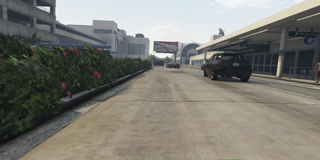
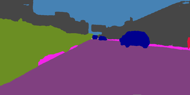
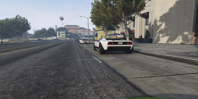
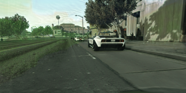
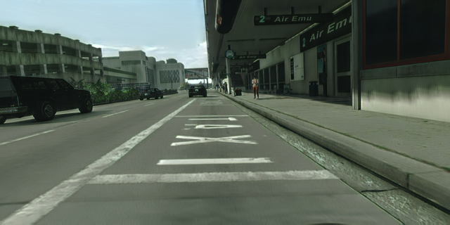
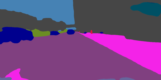
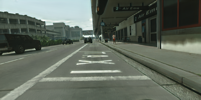
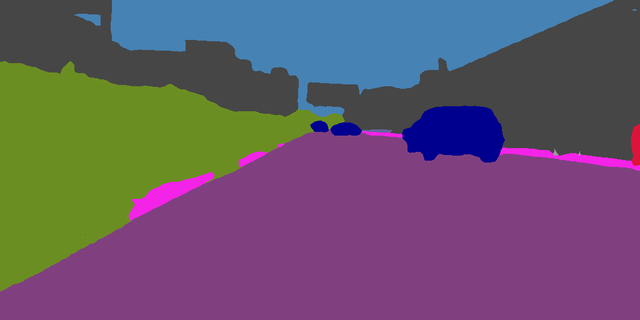
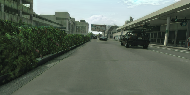
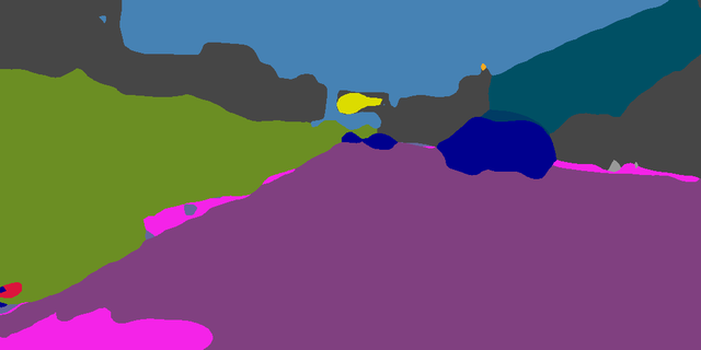
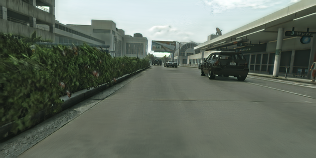
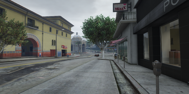
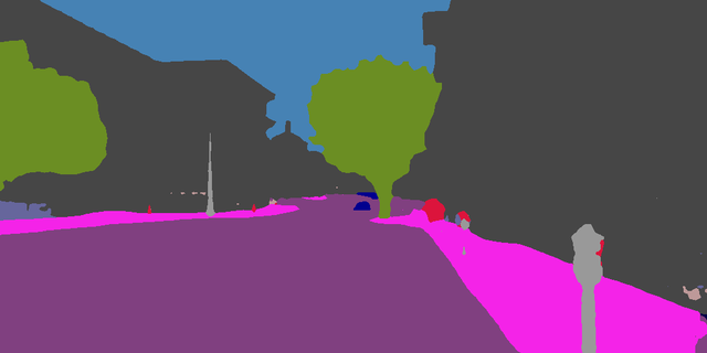
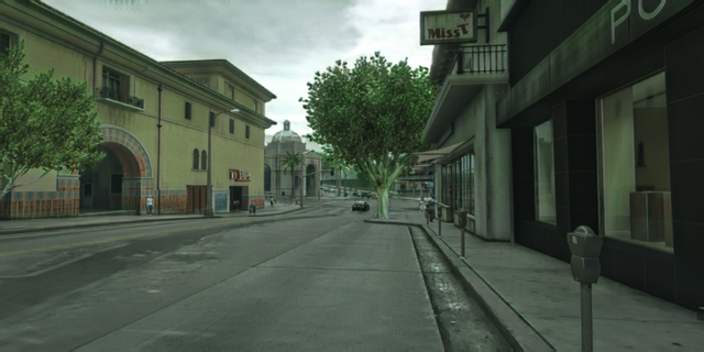
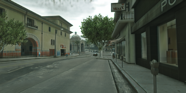
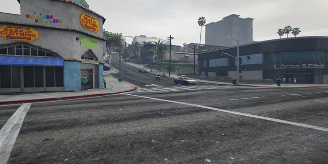
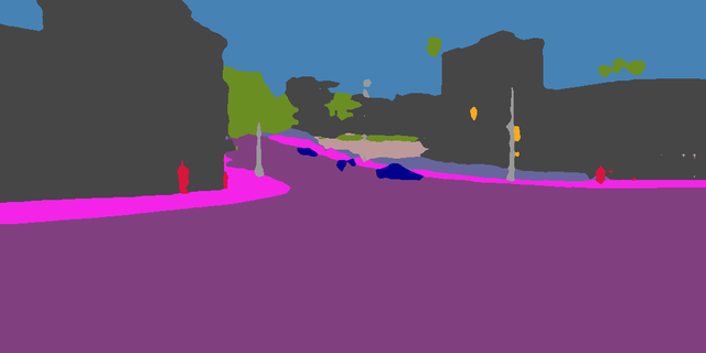
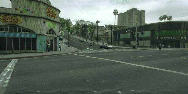
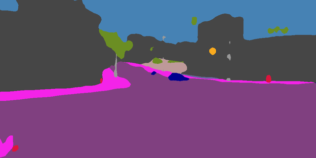
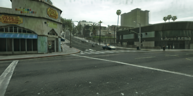
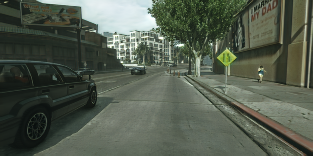
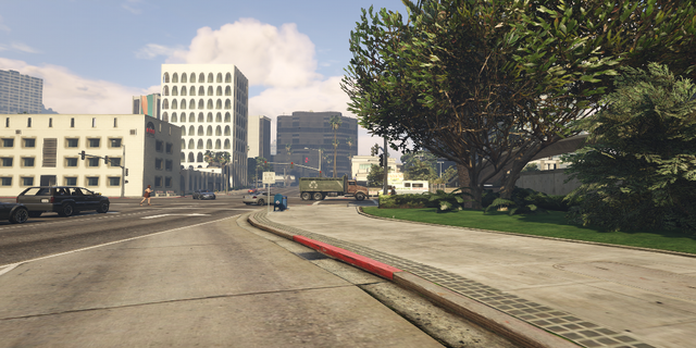
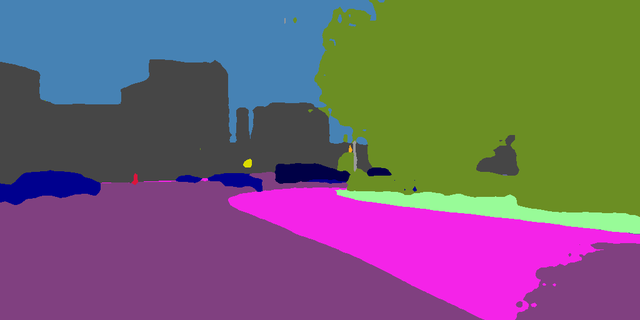
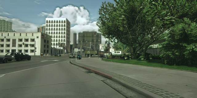
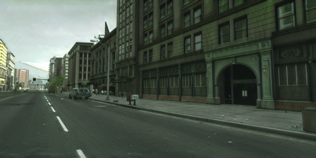
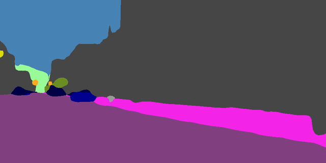
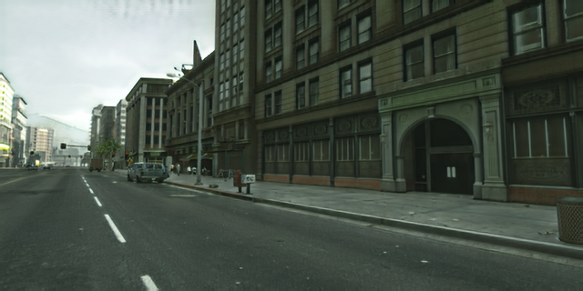
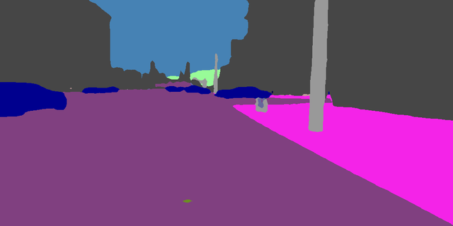
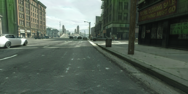
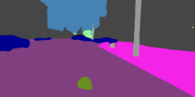
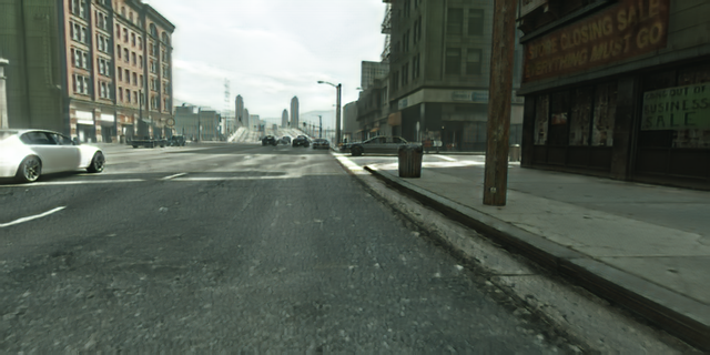
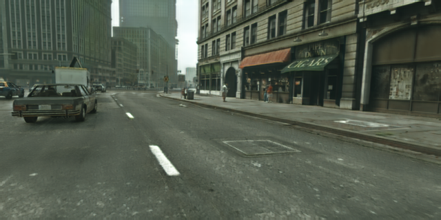
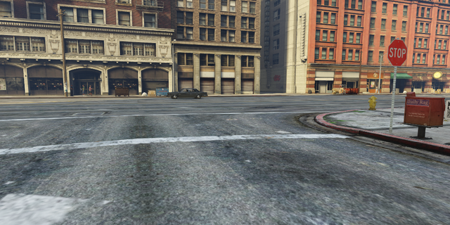
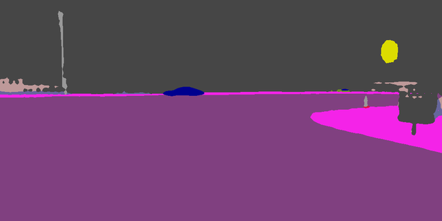
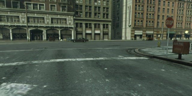
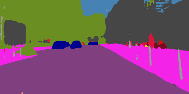
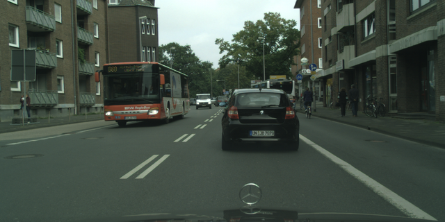
The effect of using the SPADE layers in the image-to-image translation model can be seen better when there is a mismatch between the source image and the semantic guidance. To show this effect, we feed the SPADE layers with a segmentation map extracted from an image that is different from the one being translated. In Figure 5, we can see how the denormalization wrongly creates some features in the region of the image they do not belong to (i.e. green on the road).
 |
 |
| Source for segmentation | Semantic segmentation |
 |
 |
| Source for translation | Translated image |
Appendix D Additional results
 |
 |
 |
 |
 |
 |
 |
 |
 |
 |
 |
 |
 |
 |
 |
 |
 |
 |
 |
 |
 |
 |
 |
 |
 |
 |
 |
 |
 |
 |
 |
 |
 |
 |
 |
 |
 |
 |
 |
 |
 |
 |
 |
 |
 |
 |
 |
 |
 |
 |
 |
 |
 |
 |
 |
| GTA5 sample | GTA5 pred (D) | GTA5CS (D) | GTA5 pred (F) | GTA5CS (F) |
 |
 |
 |
 |
 |
 |
 |
 |
 |
 |
 |
 |
 |
 |
 |
 |
 |
 |
 |
 |
 |
 |
 |
 |
 |
 |
 |
 |
 |
 |
 |
 |
 |
 |
 |
 |
 |
 |
 |
 |
 |
 |
 |
 |
 |
| SYNTHIA sample | SYNTHIA pred (D) | SYNTHIACS (D) | SYNTHIA pred (F) | SYNTHIACS (F) |
 |
 |
 |
 |
 |
 |
 |
 |
 |
 |
 |
 |
 |
 |
 |
 |
 |
 |
 |
 |
 |
 |
 |
 |
 |
 |
 |
 |
 |
 |
 |
 |
 |
 |
 |
 |
 |
 |
 |
 |
 |
 |
 |
 |
 |
 |
 |
 |
 |
 |
 |
 |
 |
 |
 |
 |
 |
 |
 |
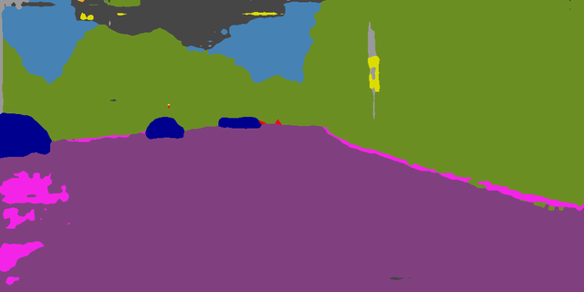 |
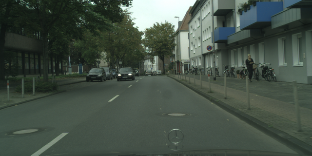
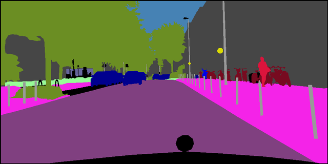
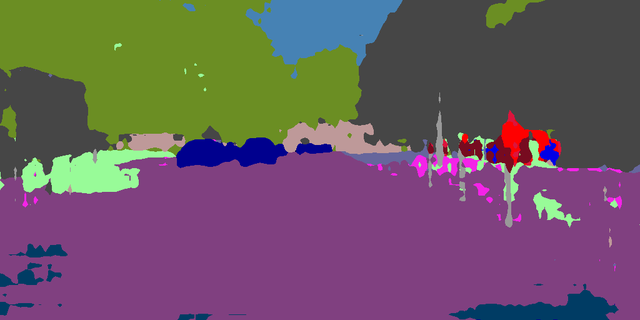
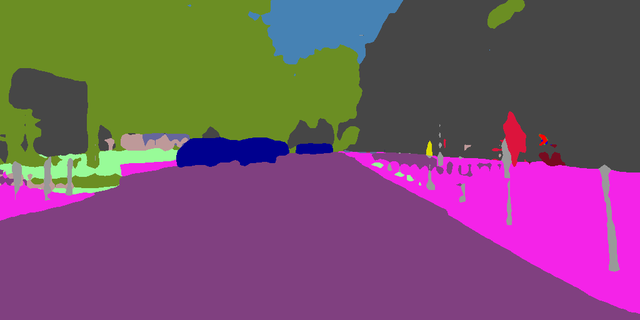
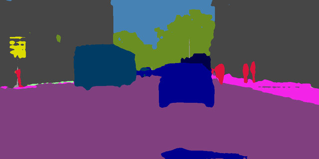
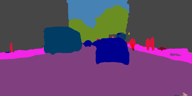
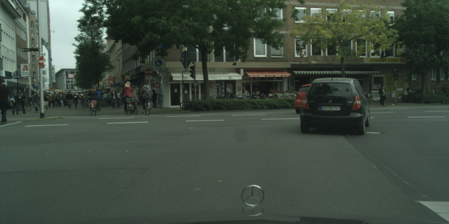
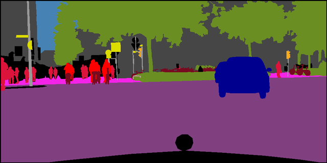
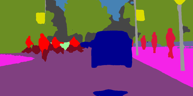
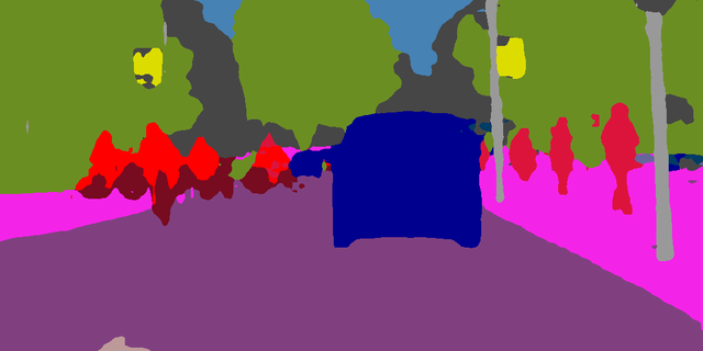
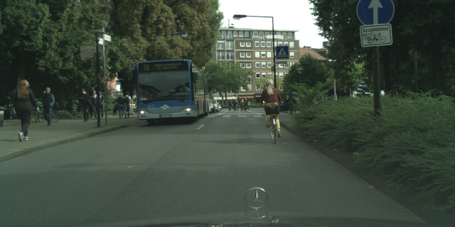
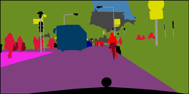
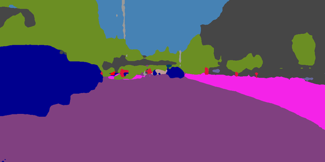
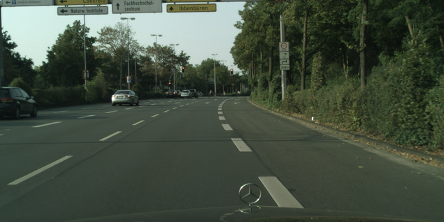
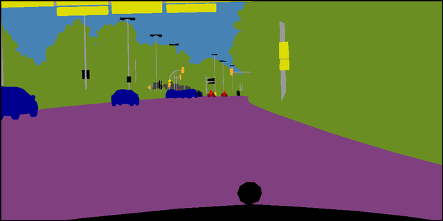
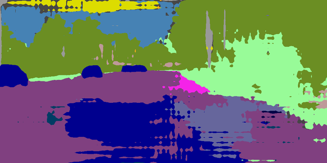
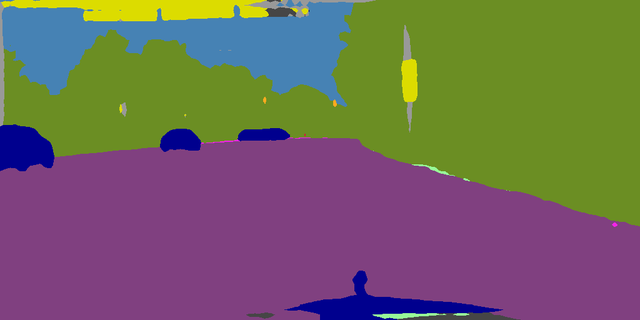
| CS sample | Ground truth | No adaptation (GTA) | GTA5CS | SYNTHIACS |