Structured eigenvalue problems in electronic structure methods from a unified perspective

Abstract

In (relativistic) electronic structure methods, the quaternion matrix eigenvalue problem and the linear response (Bethe-Salpeter) eigenvalue problem for excitation energies are two frequently encountered structured eigenvalue problems. While the former problem was thoroughly studied, the later problem in its most general form, namely, the complex case without assuming the positive definiteness of the electronic Hessian, is not fully understood. In view of their very similar mathematical structures, we examined these two problems from a unified point of view. We showed that the identification of Lie group structures for their eigenvectors provides a framework to design diagonalization algorithms as well as numerical optimizations techniques on the corresponding manifolds. By using the same reduction algorithm for the quaternion matrix eigenvalue problem, we provided a necessary and sufficient condition to characterize the different scenarios, where the eigenvalues of the original linear response eigenvalue problem are real, purely imaginary, or complex. The result can be viewed as a natural generalization of the well-known condition for the real matrix case.

I Introduction

There are two frequently appeared structured eigenvalue problems in (relativistic) electronic structure methods, which can be written into a unified way as

$$\mathbf{M}_{s}\mathbf{z} = \mathbf{z}\,\omega,\quad s=\pm 1,$$

$$\mathbf{M}_{s} = \left[\begin{array}[]{cc}\mathbf{A}&\mathbf{B}\\ -\mathbf{B}^{*}&s\mathbf{A}^{*}\\ \end{array}\right],\quad\mathbf{z}=\left[\begin{array}[]{cc}\mathbf{x}\\ \mathbf{y}\\ \end{array}\right],$$ (5)

$$\mathbf{A}^{\dagger} = \mathbf{A},\quad\mathbf{B}^{T}=-s\mathbf{B},$$ (6)

where $\mathbf{M}_{s}\in\mathbb{C}^{2n\times 2n}$, $\mathbf{z}\in\mathbb{C}^{2n}$, $\mathbf{A}\in\mathbb{C}^{n\times n}$ is Hermitian, and $\mathbf{B}\in\mathbb{C}^{n\times n}$ is antisymmetric for $s=+1$ or symmetric for $s=-1$.

The $s=+1$ case appears in matrix representations of Hermitian operators, such as the Fock operator of closed-shell systems, in a Kramers paired basis¹. Another example is the equation-of-motion method² for ionization and electron attachment from a closed-shell reference, where the excitation operator $O_{n}^{\dagger}$ is expanded in a paired basis $\{a_{p}^{\dagger},a_{p}\}$, viz., $O_{n}^{\dagger}=\sum_{p}(a_{p}^{\dagger}X_{p}-a_{q}Y_{p})$. The Hermitian matrix $\mathbf{M}_{+}$ is usually referred as quaternion matrix^{3, 4, 5}, since it can be rewritten as

$$\mathbf{M}_{+}=\mathbf{I}_{2}\otimes\mathbf{A}_{\mathrm{R}}+i\sigma_{z}\otimes\mathbf{A}_{\mathrm{I}}+i\sigma_{y}\otimes\mathbf{B}_{\mathrm{R}}+i\sigma_{x}\otimes\mathbf{B}_{\mathrm{I}}.$$ (7)

where $\{\mathbf{I}_{2},i\sigma_{z},i\sigma_{y},i\sigma_{x}\}$ is isomorphic to the set of quaternion units $\{1,\breve{i},\breve{j},\breve{k}\}$, where $\mathbf{A}_{\mathrm{R}}$ (or $\mathbf{A}_{\mathrm{I}}$) represents the real (or imaginary) part of $\mathbf{A}$. The corresponding eigenvalue problem is well-studied, and several efficient algorithms have been presented^{3, 6, 4, 5, 7}, based on the generalization of established algorithms for complex matrices to quaternion algebra or the use of unitary symplectic transformations.

The $s=-1$ case appears in the linear response problem^{8, 9, 10, 11, 12, 13, 14, 15, 16, 17} for excitation energies of Hartree-Fock (HF), density functional theory (DFT), multi-configurational self-consistent field (MCSCF), or the Bethe-Salpeter equation (BSE)¹⁸. Compared with the $s=1$ case, the linear response eigenvalue problem is more challenging since $\mathbf{M}_{-}$ is non-Hermitian. In practice, we are mostly interested in the real eigenvalues, which correspond to physical excitation energies. Unfortunately, the condition for the existence of all real eigenvalues is only partially understood. In the nonrelativistic¹⁹ and some relativistic cases¹⁶, where $\mathbf{M}_{-}$ becomes real, the eigenvalue problem (6) is equivalent to the reduced problem

$$(\mathbf{A}-\mathbf{B})(\mathbf{A}+\mathbf{B})(\mathbf{x}+\mathbf{y})=(\mathbf{x}+\mathbf{y})\omega^{2},$$ (8)

or

$$(\mathbf{A}+\mathbf{B})(\mathbf{A}-\mathbf{B})(\mathbf{x}-\mathbf{y})=(\mathbf{x}-\mathbf{y})\omega^{2}.$$ (9)

Thus, the eigenvalues of the original problem are all real if and only if the eigenvalues of the reduced matrix $(\mathbf{A}-\mathbf{B})(\mathbf{A}+\mathbf{B})$ (or its transpose $(\mathbf{A}+\mathbf{B})(\mathbf{A}-\mathbf{B})$) are all nonnegative, i.e., $\omega^{2}\geq 0$. Besides, the use of Eq. (8) or (9) also reduces the cost for diagonalization compared with that for Eq. (6). If $\mathbf{M}_{-}$ is complex as in the relativistic case in general, such reduction is not possible. Assuming the positive definiteness of the so-called electronic Hessian,

$$\left[\begin{array}[]{cc}\mathbf{A}&\mathbf{B}\\ \mathbf{B}^{*}&\mathbf{A}^{*}\\ \end{array}\right]\succ 0,$$ (12)

one can show that all eigenvalues of $\mathbf{M}_{-}$ are real^{20, 21, 22}. However, this condition is only a sufficient condition. In the real case, this implies $\mathbf{A}-\mathbf{B}\succ 0$ and $\mathbf{A}+\mathbf{B}\succ 0$. Another sufficient condition is $\mathbf{B}=0$, in which case $\mathbf{M}_{-}$ is block-diagonal and all its eigenvalues are real, even though there can be negative eigenvalues in $\mathbf{A}$. The situation, where the electronic Hessian is not positive definite but $\mathbf{M}_{-}$ still have all real eigenvalues, is also practically meaningful. It happens in using an excited state as reference, a trick that has been commonly used in time-dependent DFT to treat excited states of systems with a spatially degenerate ground state²³. Besides, it also happens in scanning the potential energy curves, where a curve crossing is encountered between the ground and an excited state with a different symmetry²⁴. In such cases, the negative eigenvalues correspond to de-excitations to a lower energy state.

Due to the similarity in mathematical structures for the $s=1$ and $s=-1$ cases, in this work we examine these two problems from a unified perspective. We first identify the Lie group structures for their eigenvectors (see Sec. II). Then, by using the same reduction algorithm for the $s=1$ case (see Sec. III), we provide a condition as a generalization of the real case based on the reduced problems (Eqs. (8) and (9)) to characterize the different scenarios, where the eigenvalues of the complex linear response problem are real, purely imaginary, or complex (see Sec. IV). Some typical examples are provided in Sec. V to illustrate the complexity of the eigenvalue problem (6) in the $s=-1$ case.

II Lie group structures of the eigensystems

The matrices in Eq. (6) with $s=1$ and $s=-1$ are closely related with the skew-Hamiltonian matrix $\mathbf{W}$ and Hamiltonian matrix $\mathbf{H}$ in real field²⁵, respectively,

$$\mathbf{W} = \left[\begin{array}[]{cc}\mathbf{W}_{11}&\mathbf{W}_{12}\\ \mathbf{W}_{21}&\mathbf{W}_{11}^{T}\\ \end{array}\right],\;\mathbf{W}_{12}=-\mathbf{W}_{12}^{T},\;\mathbf{W}_{21}=-\mathbf{W}_{21}^{T},$$ (15)

$$\mathbf{H} = \left[\begin{array}[]{cc}\mathbf{H}_{11}&\mathbf{H}_{12}\\ \mathbf{H}_{21}&-\mathbf{H}_{11}^{T}\\ \end{array}\right],\;\mathbf{H}_{12}=\mathbf{H}_{12}^{T},\;\mathbf{H}_{21}=\mathbf{H}_{21}^{T}.$$ (18)

The identification of the Hamiltonian structure for the linear response problem was presented in Ref. ²⁶ for the real matrix case. It can be shown that the eigenvalues of $\mathbf{W}$ appear in pairs $\{\omega,\omega\}$, while the eigenvalues of $\mathbf{H}$ appear in pairs $\{\omega,-\omega\}$²⁵. The same results also hold for complex matrices. Besides, the additional relations with complex conjugation in Eq. (6) compared with Eqs. (15) and (18), viz., $\mathbf{W}_{21}=-\mathbf{W}_{12}^{*}=-\mathbf{B}^{*}$, $\mathbf{W}_{11}^{T}=\mathbf{W}_{11}^{*}=\mathbf{A}^{*}$, $\mathbf{H}_{21}=-\mathbf{H}_{12}^{*}=-\mathbf{B}^{*}$, and $\mathbf{H}_{11}^{T}=\mathbf{H}_{11}^{*}=\mathbf{A}^{*}$, lead to further structures on eigenvalues and eigenvectors,

$$\mathbf{Z}_{s}=\left[\begin{array}[]{cc}\mathbf{X}&-s\mathbf{Y}^{*}\\ \mathbf{Y}&\mathbf{X}^{*}\\ \end{array}\right],\quad\bm{\omega}_{s}=\left[\begin{array}[]{cc}\bm{\omega}&\mathbf{0}\\ \mathbf{0}&s\bm{\omega}^{*}\\ \end{array}\right].$$ (23)

Thus, the symmetry relationships among eigenvalues of Eq. (6) can be deducted. For $s=1$, the eigenvalues are real doubly degenerate $\{\omega,\omega=\omega^{*}\}$, which is a reflection of the time reversal symmetry. For $s=-1$, the quadruple of eigenvalues $\{\omega,-\omega,\omega^{*},-\omega^{*}\}$ appears. If $\omega=\omega^{*}$ (or $-\omega^{*}$) is real (purely imaginary), then the quadruple reduces to the pair $\{\omega,-\omega\}$. Note that the pair structure (23) always holds for $s=1$, since $(\mathbf{X},\mathbf{Y})$ and $(-\mathbf{Y}^{*},\mathbf{X}^{*})$ are orthogonal. However, for $s=-1$, the situation becomes more complicated in the degenerate case $\omega=-\omega^{*}$, where the pair structure of eigenvectors does not necessarily hold. The following discussion in this section only works for the $s=-1$ case where all the eigenvectors have the pair structure (23), while the algorithm presented in Sec. IV does not have this assumption.

While most of the previous studies focused on the paired structure (23) for a given matrix $\mathbf{M}_{s}$, we note that if the set of matrices with the same form as the eigenvectors $\mathbf{Z}_{s}$ (23) is considered, along with the commonly applied normalization conditions,

$$\mathbf{Z}^{\dagger}_{s}\mathbf{N}_{s}\mathbf{Z}_{s}=\mathbf{N}_{s},\quad\mathbf{N}_{s}=\left[\begin{array}[]{cc}\mathbf{I}_{n}&\mathbf{0}\\ \mathbf{0}&s\mathbf{I}_{n}\end{array}\right],$$ (26)

these matrices actually form matrix groups, viz.,

$$\mathcal{G}_{s}=\{\mathbf{Z}_{s}:\,\mathbf{Z}_{s}=\left[\begin{array}[]{cc}\mathbf{X}&-s\mathbf{Y}^{*}\\ \mathbf{Y}&\mathbf{X}^{*}\\ \end{array}\right],\,\mathbf{Z}^{\dagger}_{s}\mathbf{N}_{s}\mathbf{Z}_{s}=\mathbf{N}_{s}\}.$$ (29)

This can be simply verified by following the definition of groups as follows:

(1) This set is closed under multiplication of two matrices, since

$$\mathbf{Z}_{s,1}\mathbf{Z}_{s,2} = \left[\begin{array}[]{cc}\mathbf{X}_{1}&-s\mathbf{Y}^{*}_{1}\\ \mathbf{Y}_{1}&\mathbf{X}^{*}_{1}\\ \end{array}\right]\left[\begin{array}[]{cc}\mathbf{X}_{2}&-s\mathbf{Y}^{*}_{2}\\ \mathbf{Y}_{2}&\mathbf{X}^{*}_{2}\\ \end{array}\right]$$ (34)

$$= \left[\begin{array}[]{cc}\mathbf{X}_{1}\mathbf{X}_{2}-s\mathbf{Y}^{*}_{1}\mathbf{Y}_{2}&-s(\mathbf{X}_{1}\mathbf{Y}^{*}_{2}+\mathbf{Y}^{*}_{1}\mathbf{X}^{*}_{2})\\ \mathbf{X}^{*}_{1}\mathbf{Y}_{2}+\mathbf{Y}_{1}\mathbf{X}_{2}&\mathbf{X}^{*}_{1}\mathbf{X}^{*}_{2}-s\mathbf{Y}_{1}\mathbf{Y}^{*}_{2}\\ \end{array}\right]$$ (37)

$$\triangleq \left[\begin{array}[]{cc}\mathcal{X}&-s\mathcal{Y}^{*}\\ \mathcal{Y}&\mathcal{X}^{*}\\ \end{array}\right],$$ (40)

and $(\mathbf{Z}_{s,1}\mathbf{Z}_{s,2})^{\dagger}\mathbf{N}_{s}(\mathbf{Z}_{s,1}\mathbf{Z}_{s,2})=\mathbf{N}_{s}$, that is $\mathbf{Z}_{s,1}\mathbf{Z}_{s,2}\in\mathcal{G}_{s}$.

(2) The identity element is just $\mathbf{I}_{2n}$.

(3) The inverse of any element $\mathbf{Z}_{s}$ exists, since $\mathbf{Z}_{s}$ satisfies the normalization condition (26),

$$\mathbf{Z}_{s}^{-1}=\mathbf{N}_{s}\mathbf{Z}_{s}^{\dagger}\mathbf{N}_{s}=\left[\begin{array}[]{cc}\mathbf{X}^{\dagger}&s\mathbf{Y}^{\dagger}\\ -\mathbf{Y}^{T}&\mathbf{X}^{T}\end{array}\right]\in\mathcal{G}_{s}.$$ (43)

In fact, the groups (29) are just the unitary symplectic Lie groups, viz., $\mathrm{USp}(2n)=\mathrm{U}(2n)\cap\mathrm{Sp}(2n,\mathbb{C})$ for $s=+1$, and $\mathrm{USp}(n,n)=\mathrm{U}(n,n)\cap\mathrm{Sp}(2n,\mathbb{C})$ for $s=-1$. Here, $\mathrm{U}(p,q)$ represents the unitary group with signature $(p,q)$, i.e.,

$$\mathbf{U}(p,q)=\{\mathbf{M}:\;\mathbf{M}^{\dagger}\mathbf{I}_{p,q}\mathbf{M}=\mathbf{I}_{p,q}\},\;\;\mathbf{I}_{p,q}=\left[\begin{array}[]{cc}\mathbf{I}_{p}&\mathbf{0}\\ \mathbf{0}&-\mathbf{I}_{q}\\ \end{array}\right],$$ (46)

and $\mathrm{Sp}(2n,\mathbb{C})$ represents the complex symplectic group,

$$\mathrm{Sp}(2n,\mathbb{C})=\{\mathbf{M}:\;\mathbf{M}^{T}\mathbf{J}\mathbf{M}=\mathbf{J}\},\;\;\mathbf{J}=\left[\begin{array}[]{cc}\mathbf{0}&\mathbf{I}_{n}\\ -\mathbf{I}_{n}&\mathbf{0}\\ \end{array}\right].$$ (49)

Such equivalence can be established by realizing that a combination of the conditions in Eqs. (46) and (49) leads to a condition

$$\mathbf{J}_{s}\mathbf{M}^{*}=\mathbf{M}\mathbf{J}_{s},\quad\mathbf{J}_{s}=\left[\begin{array}[]{cc}\mathbf{0}&\mathbf{I}_{n}\\ -s\mathbf{I}_{n}&\mathbf{0}\\ \end{array}\right],$$ (52)

which implies the block structures in Eq. (29) for the $2n$-by-$2n$ matrix $\mathbf{M}$. Note in passing that the case $s=1$ for Eq. (52) reveals the underlying commutation between an operator and the time reversal operator.

The identification of Lie group structures for $\mathcal{G}_{s}$ has important consequences. In particular, it simplifies the design of structure-preserving algorithms. For instance, for the case $s=1$, the Lie algebra $\mathfrak{usp}(2n)$ corresponding to the Lie group $\mathrm{USp}(2n)$ is

$$\mathfrak{usp}(2n)=\{\mathbf{K}:\;\mathbf{K}^{\dagger}=-\mathbf{K},\;\mathbf{J}\mathbf{K}^{*}=\mathbf{K}\mathbf{J}\},$$ (53)

where the matrix $\mathbf{K}$ can be written more explicitly as

$$\mathbf{K}=\left[\begin{array}[]{cc}\mathbf{K}_{11}&-\mathbf{K}_{21}^{*}\\ \mathbf{K}_{21}&\mathbf{K}_{11}^{*}\\ \end{array}\right],\;\mathbf{K}_{11}^{\dagger}=-\mathbf{K}_{11},\;\mathbf{K}_{21}^{T}=\mathbf{K}_{21}.$$ (56)

This applies to the construction of time reversal adapted basis operators²⁷. Furthermore, the exponential map $\exp(\mathbf{K})$ can be used to transform one Kramers paired basis into another Kramers paired basis, which was previously used in the Kramers-restricted MCSCF²⁸. More generally, such Lie group (29) and Lie algebra structures for the case $s=1$ also implies the possibility to apply the numerical techniques for the optimization on manifolds²⁹ to relativistic spinor optimizations while preserving the Kramers pair structure. Due to the unified framework presented here, one can expect that the similar techniques can also be applied to the $s=-1$ case.

III Reduction algorithm for the $s=1$ case

In this section, we will briefly recapitulate the reduction algorithm for the $s=1$ case, by adapting the techniques developed for the real skew Hamiltonian matrices^{30, 31} to the complex matrix $\mathbf{M}_{+}$ (6). Such techniques also form basis for developing diagonalization algorithms for the relativistic Fock matrix^{6, 7}. The essential idea is to realize that the unitary symplectic transformation

$$\mathbf{G}=\left[\begin{array}[]{cc}\mathbf{U}&-\mathbf{V}^{*}\\ \mathbf{V}&\mathbf{U}^{*}\\ \end{array}\right]\in\mathrm{USp}(2n),$$ (59)

when acting on a skew Hamiltonian (complex) matrix, such as $\mathbf{W}$ (15) via $\tilde{\mathbf{W}}=\mathbf{G}\mathbf{W}\mathbf{G}^{\dagger}$, will preserve the skew-Hamiltonian structure, viz.,

$$\tilde{\mathbf{W}}_{22}=\tilde{\mathbf{W}}_{11}^{T},\;\;\tilde{\mathbf{W}}_{12}^{T}=-\tilde{\mathbf{W}}_{12},\;\;\tilde{\mathbf{W}}_{21}^{T}=-\tilde{\mathbf{W}}_{21}.$$ (60)

Then, there is a constructive way³⁰ to eliminate the lower-left block of the matrix $\mathbf{W}$ (15) by a series of unitary symplectic Householder and Givens transformations, such that the transformed matrix $\tilde{\mathbf{W}}$ is in the following Paige/Van Loan (PVL) form²⁵,

$$\tilde{\mathbf{W}}=\mathbf{G}\mathbf{W}\mathbf{G}^{\dagger}=\left[\begin{array}[]{cc}\tilde{\mathbf{W}}_{11}&\tilde{\mathbf{W}}_{12}\\ \mathbf{0}&\tilde{\mathbf{W}}_{11}^{T}\\ \end{array}\right].$$ (63)

The crucial point for being able to transform $\mathbf{W}$ into the form (63) is $\mathbf{W}_{21}=-\mathbf{W}_{21}^{T}$, and such property can be preserved during the transformations, see Ref. ³⁰ for details of the transformations. The computational scaling of such transformation is cubic in the dimension of the matrix.

Applying this result to $\mathbf{M}_{+}$ and realizing that the transformed matrix $\tilde{\mathbf{M}}_{+}$ is still Hermitian, one can conclude that $(\tilde{\mathbf{M}}_{+})_{12}=0$ and $\tilde{\mathbf{M}}_{11}^{T}=\tilde{\mathbf{M}}_{11}^{*}$, viz., $\tilde{\mathbf{M}}_{+}$ becomes block-diagonal⁷. Then, the eigenvalues can be obtained by diagonalizing the Hermitian matrix $\tilde{\mathbf{M}}_{11}$ by a unitary matrix $\bar{\mathbf{U}}$, which reduces the computational cost compared with the original problem. The final solution to the original problem can be obtained as

$$\mathbf{Z}_{+}=\mathbf{G}\left[\begin{array}[]{cc}\bar{\mathbf{U}}&\mathbf{0}\\ \mathbf{0}&\bar{\mathbf{U}}^{*}\\ \end{array}\right]=\left[\begin{array}[]{cc}\mathbf{U}\bar{\mathbf{U}}&-\mathbf{V}^{*}\bar{\mathbf{U}}\\ \mathbf{V}\bar{\mathbf{U}}^{*}&\mathbf{U}^{*}\bar{\mathbf{U}}^{*}\\ \end{array}\right]\in\mathcal{G}_{+},$$ (68)

which still preserves the structure (29) due to the closeness of groups.

IV Reduction algorithm for the $s=-1$ case

Due to the non-Hermicity of $\mathbf{M}_{-}$, a straightforward generalization of the above reduction algorithm to $\mathbf{M}_{-}$ using the transformation in $\mathrm{USp}(n,n)$ does not seem to be possible. Because the validity of the form (23) depends on the properties of the eigensystem. In some cases, $\mathbf{M}_{-}$ cannot be diagonalizable, e.g., $\mathbf{M}_{-}=\left[\begin{array}[]{cc}1&1\\ -1&-1\\ \end{array}\right]$. To avoid such difficulty, following the observation for the Hamiltonian matrix by van Loan³¹, one can find the square matrix $\mathbf{M}_{-}^{2}$ is a skew Hamiltonian matrix,

$$\mathbf{M}^{2}_{-} = \left[\begin{array}[]{cc}\mathbf{A}^{2}-\mathbf{B}\mathbf{B}^{*}&\mathbf{A}\mathbf{B}-\mathbf{B}\mathbf{A}^{*}\\ -\mathbf{B}^{*}\mathbf{A}+\mathbf{A}^{*}\mathbf{B}^{*}&(\mathbf{A}^{*})^{2}-\mathbf{B}^{*}\mathbf{B}\\ \end{array}\right]$$ (71)

$$\triangleq \left[\begin{array}[]{cc}\mathcal{A}&\mathcal{B}\\ \mathcal{B}^{*}&\mathcal{A}^{*}\\ \end{array}\right],$$ (74)

where

$$\mathcal{A} = \mathbf{A}^{2}-\mathbf{B}\mathbf{B}^{*},$$

$$\mathcal{B} = \mathbf{A}\mathbf{B}-\mathbf{B}\mathbf{A}^{*},$$

$$\mathcal{A}^{\dagger} = (\mathbf{A}^{\dagger})^{2}-\mathbf{B}^{T}\mathbf{B}^{\dagger}=\mathbf{A}^{2}-\mathbf{B}\mathbf{B}^{*}=\mathcal{A},$$

$$\mathcal{B}^{T} = \mathbf{B}^{T}\mathbf{A}^{T}-\mathbf{A}^{\dagger}\mathbf{B}^{T}=\mathbf{B}\mathbf{A}^{*}-\mathbf{A}\mathbf{B}=-\mathcal{B}.$$ (75)

Thus, it can be brought into the PVL form (63) using unitary symplectic transformations as for $\mathbf{M}_{+}$. However, it deserves to be pointed out that unlike for the Hermitian matrix $\mathbf{M}_{+}$, such transformations will not preserve the relation between the lower-left and upper-right blocks of $\mathbf{M}_{-}^{2}$, such that while $(\tilde{\mathbf{M}}^{2}_{-})_{21}$ is made zero in the transformed matrix, $(\tilde{\mathbf{M}}^{2}_{-})_{12}$ is nonzero. But the upper-left block $(\tilde{\mathbf{M}}^{2}_{-})_{11}$ can still be used to compute $\omega^{2}$ with reduced cost for diagonalization.

This basically gives a criterion for the different scenarios of eigenvalues of the linear response problem. However, to make better connection to the conditions (8) and (9) for the real case. We use the following transformation²¹,

$$\mathbf{Q}=\frac{1}{\sqrt{2}}\left[\begin{array}[]{cc}\mathbf{I}_{n}&\mathbf{I}_{n}\\ i\mathbf{I}_{n}&-i\mathbf{I}_{n}\\ \end{array}\right]$$ (78)

which transforms $\mathbf{M}_{-}$ into a purely imaginary matrix

$$\mathbf{Q}\mathbf{M}_{-}\mathbf{Q}^{\dagger}=i\left[\begin{array}[]{cc}(\mathbf{A}+\mathbf{B})_{\mathrm{I}}&-(\mathbf{A}-\mathbf{B})_{\mathrm{R}}\\ (\mathbf{A}+\mathbf{B})_{\mathrm{R}}&(\mathbf{A}-\mathbf{B})_{\mathrm{I}}\\ \end{array}\right].$$ (81)

Then, the square matrix is transformed into a real skew-Hamiltonian matrix,

$$\mathbf{\Pi}\triangleq\mathbf{Q}\mathbf{M}_{-}^{2}\mathbf{Q}^{\dagger}=\left[\begin{array}[]{cc}(\mathbf{A}-\mathbf{B})_{\mathrm{R}}(\mathbf{A}+\mathbf{B})_{\mathrm{R}}-(\mathbf{A}+\mathbf{B})_{\mathrm{I}}(\mathbf{A}+\mathbf{B})_{\mathrm{I}}&(\mathbf{A}-\mathbf{B})_{\mathrm{R}}(\mathbf{A}-\mathbf{B})_{\mathrm{I}}+(\mathbf{A}+\mathbf{B})_{\mathrm{I}}(\mathbf{A}-\mathbf{B})_{\mathrm{R}}\\ -(\mathbf{A}+\mathbf{B})_{\mathrm{R}}(\mathbf{A}+\mathbf{B})_{\mathrm{I}}-(\mathbf{A}-\mathbf{B})_{\mathrm{I}}(\mathbf{A}+\mathbf{B})_{\mathrm{R}}&(\mathbf{A}+\mathbf{B})_{\mathrm{R}}(\mathbf{A}-\mathbf{B})_{\mathrm{R}}-(\mathbf{A}-\mathbf{B})_{\mathrm{I}}(\mathbf{A}-\mathbf{B})_{\mathrm{I}}\\ \end{array}\right].$$ (84)

It is clear that if $\mathbf{M}_{-}$ is real, then $\mathbf{\Pi}$ becomes diagonal, with the diagonal blocks being simply $(\mathbf{A}-\mathbf{B})(\mathbf{A}+\mathbf{B})$ and $(\mathbf{A}+\mathbf{B})(\mathbf{A}-\mathbf{B})$, and the transformed eigenvalue problem becomes equivalent to Eqs. (8) and (9), since

$$\mathbf{Q}\mathbf{z}=\mathbf{Q}\left[\begin{array}[]{cc}\mathbf{x}\\ \mathbf{y}\\ \end{array}\right]=\frac{1}{\sqrt{2}}\left[\begin{array}[]{cc}\mathbf{x}+\mathbf{y}\\ i(\mathbf{x}-\mathbf{y})\\ \end{array}\right].$$ (89)

By applying unitary symplectic transformations to reduce $\tilde{\mathbf{\Pi}}=\mathbf{G}\mathbf{\Pi}\mathbf{G}^{\dagger}$ into the PVL form (63), the real non-Hermitian matrix $\tilde{\mathbf{\Pi}}_{11}$ can be used to compute eigenvalues of $\mathbf{M}_{-}^{2}$. Suppose the eigenvalues of $\tilde{\mathbf{\Pi}}_{11}$ are denoted by $\lambda$, then we have the following three cases:

(1) $\lambda=\lambda_{\mathrm{R}}\geq 0$: the pair of real eigenvalues of $\mathbf{M}_{-}$ is $\{\sqrt{\lambda_{\mathrm{R}}},-\sqrt{\lambda_{\mathrm{R}}}\}$.

(2) $\lambda=\lambda_{\mathrm{R}}<0$: the pair of purely imaginary eigenvalues of $\mathbf{M}_{-}$ is $\{i\sqrt{-\lambda_{\mathrm{R}}},-i\sqrt{-\lambda_{\mathrm{R}}}\}$.

(3) $\lambda=\lambda_{\mathrm{R}}+i\lambda_{\mathrm{I}}$ is complex: $\lambda^{*}=\lambda_{\mathrm{R}}-i\lambda_{\mathrm{I}}$ will also be an eigenvalue of $\tilde{\mathbf{\Pi}}_{11}$, and the quadruple of complex eigenvalues of $\mathbf{M}_{-}$ is $\{\omega,-\omega,\omega^{*},-\omega^{*}\}$ with $\omega$ given by

$$\omega=\frac{\zeta}{\sqrt{2}}+i\frac{\lambda_{\mathrm{I}}}{\sqrt{2}\zeta},\quad\zeta=\sqrt{\lambda_{\mathrm{R}}+\sqrt{\lambda_{\mathrm{R}}^{2}+\lambda_{\mathrm{I}}^{2}}}.$$ (90)

Thus, the goal to characterize the eigenvalues of the complex linear response problem in a way similar way as the real case is accomplished based on the eigenvalues of the reduced matrix $\tilde{\mathbf{\Pi}}_{11}$. In the next section, we will examine some concrete examples.

V Illustrative examples

We first illustrate the simplification due to using the square matrix $\mathbf{M}_{-}^{2}$ by considering a 2-by-2 example,

$$\mathbf{M}_{-}=\left[\begin{array}[]{cc}x&3i\\ 3i&-x\\ \end{array}\right],\;\;\mathbf{M}_{-}^{2}=\left[\begin{array}[]{cc}x^{2}-9&0\\ 0&x^{2}-9\\ \end{array}\right],$$ (95)

where $x\in\mathbb{R}$ is a parameter to mimic the effect of changing physical parameters in the linear response problem, such as the change of bond length of diatomic molecules in scanning potential energy curves. It is seen that the matrix $\mathbf{M}_{-}^{2}$ is already diagonal, which gives two identical eigenvalues $\lambda=x^{2}-9$. Consequently, the original problem have two eigenvalues $\omega=\pm\sqrt{x^{2}-9}$. The eigenvalues as a function of $x$ are shown in Fig. 1. The graphs can be classified into three regions:

(1) $x\leq-3$: $\lambda\geq 0$ and a pair of real eigenvalues $\omega=\pm\sqrt{x^{2}-9}$ appears, although the electronic Hessian is not positive definite.

(2) $-3<x<3$: $\lambda<0$ and a pair of purely imaginary eigenvalue $\omega=\pm i\sqrt{9-x^{2}}$ appear.

(3) $x\geq 3$: $\lambda\geq 0$ and the electronic Hessian is positive definite.

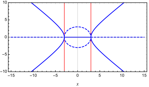
(a) $\omega$ as a function of $x$

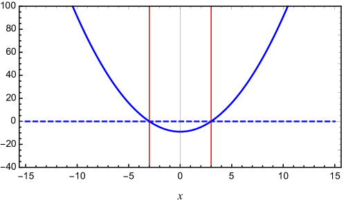
(b) $\lambda$ as a function of $x$

Figure 1: A 2-by-2 example for $\mathbf{M}_{-}$ (95): (a) eigenvalues of $\mathbf{M}_{-}$ (denoted by $\omega$) as a function of $x$; (b) eigenvalues of $\mathbf{M}_{-}^{2}$ (denoted by $\lambda$) as a function of $x$. The blue solid (dashed) lines represent the real (imaginary) parts of eigenvalues. The two red vertical lines represent critical values of $x=\pm 3$.

Next, we examine a more complex example, which covers all the scenarios for eigenvalues of $\mathbf{M}_{-}$. The matrices $\mathbf{A}$ and $\mathbf{B}$ are chosen as

$$\mathbf{A}=\left[\begin{array}[]{cc}x&3+i\\ 3-i&5\\ \end{array}\right],\quad\mathbf{B}=\left[\begin{array}[]{cc}4&4\\ 4&4\\ \end{array}\right].$$ (100)

The eigenvalues of $\mathbf{M}_{-}$ can be found analytically as

$$\omega = \pm\sqrt{\frac{-19+x^{2}\pm\sqrt{\Delta}}{2}},$$

$$\Delta = 25+272x-74x^{2}+x^{4}.$$ (101)

Following the procedure described in the previous section, one can find the corresponding skew-Hamiltonian $\mathbf{\Pi}$ (84) as

$$\mathbf{\Pi}=\left[\begin{array}[]{cccc}-22+x^{2}&-37+7x&0&-3+x\\ 3-x&3&3-x&0\\ 0&-13-x&-22+x^{2}&3-x\\ 13+x&0&-37+7x&3\\ \end{array}\right]$$ (106)

Applying the following Givens rotation $\mathbf{G}$ with an appropriate angle $\theta$ to eliminate $\Pi_{41}$,

$$\mathbf{G}=\left[\begin{array}[]{cccc}1&0&0&0\\ 0&\cos\theta&0&-\sin\theta\\ 0&0&1&0\\ 0&\sin\theta&0&\cos\theta\\ \end{array}\right],$$ (111)

we can find the upper-left block of $\tilde{\mathbf{\Pi}}=\mathbf{G}\mathbf{\Pi}\mathbf{G}^{\dagger}$ as

$$\tilde{\mathbf{\Pi}}_{11}=\left[\begin{array}[]{cc}-22+x^{2}&\frac{\sqrt{2}(-3+x)(-25+3x)}{\sqrt{89+10x+x^{2}}}\\ -\sqrt{2(89+10x+x^{2})}&3\\ \end{array}\right].$$ (114)

It can be verified that its two eigenvalues are given by $\lambda_{\pm}=\frac{-19+x^{2}\pm\sqrt{\Delta}}{2}$, which is consistent with Eq. (101). As shown in Fig. 2, the eigenvalues $\omega$ and $\lambda$ as a function of $x$ are much more complicated in this example. The conditions $\Delta=0$ and $\lambda_{\pm}=0$ determine four real critical values of $x$ in total, viz.,

$$x_{1}\approx-10.04,\quad x_{2}\approx-0.09,$$

$$x_{3}=\frac{14}{9}\approx 1.56,\quad x_{4}=6.$$ (115)

Consequently, the graphs can be classified into five regions:

(1) $x\leq x_{1}$: $\lambda_{+}\geq\lambda_{-}>0$ and $\mathbf{M}_{-}$ has two pairs of real eigenvalues.

(2) $x_{1}<x<x_{2}$: $\lambda_{+}=\lambda_{-}^{*}$ become complex, such that $\mathbf{M}_{-}$ has a quadruple of eigenvalues.

(3) $x_{2}\leq x<x_{3}$: $0>\lambda_{+}\geq\lambda_{-}$ and $\mathbf{M}_{-}$ has two pairs of purely imaginary eigenvalues.

(4) $x_{3}\leq x<x_{4}$: $\lambda_{+}\geq 0>\lambda_{-}$ and $\mathbf{M}_{-}$ has a pair of real eigenvalues and a pair of purely imaginary eigenvalues.

(5) $x\geq x_{4}$: $\lambda_{+}>\lambda_{-}\geq 0$ and $\mathbf{M}_{-}$ has two pairs of real eigenvalues.

This example covers all the three different scenarios of eigenvalues of $\mathbf{M}_{-}$ discussed in the previous section. All of them can be easily characterized by eigenvalues of a simpler matrix $\tilde{\mathbf{\Pi}}_{11}$ with halved dimension, which is a natural generalization of $(\mathbf{A}-\mathbf{B})(\mathbf{A}+\mathbf{B})$ or $(\mathbf{A}+\mathbf{B})(\mathbf{A}-\mathbf{B})$ in the real case. Finally, we mention that for larger matrices, the eigenvalues cannot be computed analytically, but it is straightforward to implement the reduction procedure numerically. The behaviors of eigenvalues can be understood in the same way following the examples presented here.

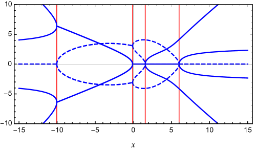
(a) $\omega$ as a function of $x$

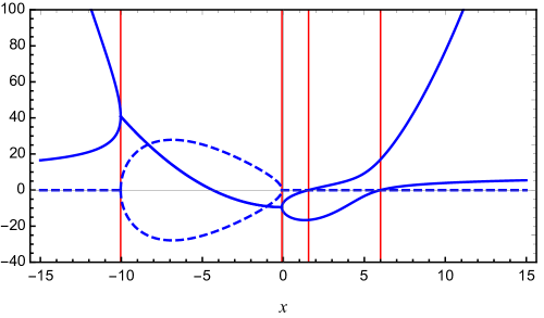
(b) $\lambda$ as a function of $x$

Figure 2: A 4-by-4 example for $\mathbf{M}_{-}$ (100): (a) eigenvalues of $\mathbf{M}_{-}$ (denoted by $\omega$) as a function of $x$; (b) eigenvalues of $\mathbf{M}_{-}^{2}$ (denoted by $\lambda$) as a function of $x$. The blue solid (dashed) lines represent the real (imaginary) parts of eigenvalues. The four red vertical lines represent critical values of $x$ given in Eq. (115).

VI Conclusion

In this work, we provided a unified view for the two commonly appeared structured eigenvalue problems in (relativistic) electronic structure methods - the quaternion matrix eigenvalue problem and the linear response eigenvalue problem for excitation energies. Using the same reduction algorithm, we derived a generalized condition to characterize the different scenarios for eigenvalues of the complex linear response problem. Such understandings may allow to design more efficient and robust diagonalization algorithms in future.

References

- Dyall and Fægri Jr 2007 K. G. Dyall and K. Fægri Jr, Introduction to relativistic quantum chemistry (Oxford University Press, 2007).
- Rowe 1968 D. J. Rowe, Reviews of Modern Physics 40, 153 (1968).
- Rösch 1983 N. Rösch, Chemical Physics 80, 1 (1983).
- Bunse-Gerstner et al. 1989 A. Bunse-Gerstner, R. Byers, and V. Mehrmann, Numerische Mathematik 55, 83 (1989).
- Saue and Jensen 1999 T. Saue and H. A. Jensen, The Journal of Chemical Physics 111, 6211 (1999).
- Dongarra et al. 1984 J. Dongarra, J. Gabriel, D. Koelling, and J. Wilkinson, Linear Algebra and its Applications 60, 27 (1984).
- Shiozaki 2017 T. Shiozaki, Molecular Physics 115, 5 (2017).
- 8 J. Olsen and P. Jørgensen, The Journal of Chemical Physics 82.
- Olsen et al. 1988 J. Olsen, H. J. A. Jensen, and P. Jørgensen, Journal of Computational Physics 74, 265 (1988).
- Sasagane et al. 1993 K. Sasagane, F. Aiga, and R. Itoh, The Journal of Chemical Physics 99, 3738 (1993).
- Christiansen et al. 1998 O. Christiansen, P. Jørgensen, and C. Hättig, International Journal of Quantum Chemistry 68, 1 (1998).
- Casida 1995 M. E. Casida, Recent Advances in Density Functional Methods, edited by D. P. Chang, Vol. 1 (World Scientific, Singapore, 1995) p. 155.
- Gao et al. 2004 J. Gao, W. Liu, B. Song, and C. Liu, The Journal of Chemical Physics 121, 6658 (2004).
- Bast et al. 2009 R. Bast, H. J. A. Jensen, and T. Saue, International Journal of Quantum Chemistry 109, 2091 (2009).
- Egidi et al. 2016 F. Egidi, J. J. Goings, M. J. Frisch, and X. Li, Journal of Chemical Theory and Computation 12, 3711 (2016).
- Liu and Xiao 2018 W. Liu and Y. Xiao, Chemical Society Reviews 47, 4481 (2018).
- Komorovsky et al. 2019 S. Komorovsky, P. J. Cherry, and M. Repisky, The Journal of Chemical Physics 151, 184111 (2019).
- Salpeter and Bethe 1951 E. E. Salpeter and H. A. Bethe, Physical Review 84, 1232 (1951).
- Stratmann et al. 1998 R. E. Stratmann, G. E. Scuseria, and M. J. Frisch, The Journal of Chemical Physics 109, 8218 (1998).
- Shao and Yang 2015 M. Shao and C. Yang, in International Workshop on Eigenvalue Problems: Algorithms, Software and Applications in Petascale Computing (Springer, 2015) pp. 91–105.
- Shao et al. 2016 M. Shao, H. Felipe, C. Yang, J. Deslippe, and S. G. Louie, Linear Algebra and its Applications 488, 148 (2016).
- Benner et al. 2018 P. Benner, H. Faßbender, and C. Yang, Linear Algebra and its Applications 544, 407 (2018).
- Seth and Ziegler 2005 M. Seth and T. Ziegler, The Journal of Chemical Physics 123, 144105 (2005).
- Li et al. 2011 Z. Li, W. Liu, Y. Zhang, and B. Suo, The Journal of Chemical Physics 134, 134101 (2011).
- Kressner 2005 D. Kressner, Numerical Methods for General and Structured Eigenvalue Problems, Vol. 46 (Springer-Verlag, Berlin, 2005).
- List et al. 2014 N. H. List, S. Coriani, O. Christiansen, and J. Kongsted, The Journal of Chemical Physics 140, 224103 (2014).
- Aucar et al. 1995 G. Aucar, H. A. Jensen, and J. Oddershede, Chemical Physics letters 232, 47 (1995).
- Fleig et al. 1997 T. Fleig, C. M. Marian, and J. Olsen, Theoretical Chemistry Accounts 97, 125 (1997).
- Absil et al. 2009 P.-A. Absil, R. Mahony, and R. Sepulchre, Optimization algorithms on matrix manifolds (Princeton University Press, 2009).
- Paige and Van Loan 1981 C. Paige and C. Van Loan, Linear Algebra and its Applications 41, 11 (1981).
- Van Loan 1984 C. Van Loan, Linear algebra and its applications 61, 233 (1984).