Receiver Design for OTFS with
Fractionally Spaced Sampling Approach

Abstract

The recent emergence of orthogonal time frequency space (OTFS) modulation as a novel PHY-layer mechanism is more suitable in high-mobility wireless communication scenarios than traditional orthogonal frequency division multiplexing (OFDM). Although multiple studies have analyzed OTFS performance using theoretical and ideal baseband pulseshapes, a challenging and open problem is the development of effective receivers for practical OTFS systems that must rely on non-ideal pulseshapes for transmission. This work focuses on the design of practical receivers for OTFS. We consider a fractionally spaced sampling (FSS) receiver in which the sampling rate is an integer multiple of the symbol rate. For rectangular pulses used in OTFS transmission, we derive a general channel input-output relationship of OTFS in delay-Doppler domain without the common reliance on impractical assumptions such as ideal bi-orthogonal pulses and on-the-grid delay/Doppler shifts. We propose two equalization algorithms: iterative combining message passing (ICMP) and turbo message passing (TMP) for symbol detection by exploiting delay-Doppler channel sparsity and the channel diversity gain via FSS. We analyze the convergence performance of TMP receiver and propose simplified message passing (MP) receivers to further reduce complexity. Our FSS receivers demonstrate stronger performance than traditional receivers and robustness to the imperfect channel state information knowledge.

I Introduction

In widespread development of wireless networks, high-mobility applications such as high-speed trains and autonomous vehicles pose new challenges due to the well-known obstacle of time-varying channels with high Doppler spread. Even though orthogonal frequency division multiplexing (OFDM) modulation has achieved high spectral efficiency and throughput for slow fading frequency selective channels, its performance degrades significantly against faster time-varying channels because of the loss of orthogonality or inter-carrier-interference (ICI) among OFDM subcarriers. One solution is to shorten OFDM symbol duration so that the channel appears quasi-stationary over each OFDM symbol [1], but at the cost of lower spectral efficiency caused by the more significant cyclic prefix (CP). Another approach is to mitigate ICI [2, 3, 4], which, however, is only effective for low or medium Doppler shifts and may incur some performance loss. In addition, [5] proposes a frequency-domain multiplexing with frequency-domain cyclic prefix (FDM-FDCP) scheme, which can efficiently tackle the Doppler spread but cannot handle the multipath delay effect resulting in inter-symbol interference (ISI).

Recently, orthogonal time frequency space (OTFS) has emerged [6] as a promising PHY-layer modulation for high-mobility scenarios. OTFS can exploit the degrees of freedom in both the delay and Doppler dimensions of a mobile wireless channel, resulting in superior performance compared with OFDM. A number of studies on OTFS have been published for multiple-input multiple-output (MIMO) system [7], multiple access system [8, 9] and for radar [10, 11]. Works by [12] and [13][14] analyzed the diversity gain of OTFS system in static multipath channels and doubly dispersive channels, respectively. Furthermore, the authors of [15] analyzed the peak-to-average power ratio (PAPR) of OTFS whereas the authors of [16] studied the pulse shaping effect of OTFS.

Unlike OFDM, OTFS multiplexes information symbols in the 2-dimensional (2D) delay-Doppler domain instead of the time-frequency domain. Thus, a channel that rapidly varies in time-frequency domain is transformed into a near stationary channel in the delay-Doppler domain. This near stationary channel simplifies not only the receiver design [17, 13, 18] but also the process of channel estimation [19, 20, 18] for OTFS systems in high-mobility scenarios. However, most existing works [18, 6, 13, 7, 17, 8, 9] only consider the use of the ideal bi-orthogonal pulses that admit a simple input-output channel relationship in the delay-Doppler domain for efficient receiver design. Unfortunately, such ideal pulses are not realizable in practice due to the Heisenberg uncertainty principle [21]. Alternatively, an OFDM-based OTFS system [22, 23, 24, 25] may utilize the practical rectangular pulses. However, this OFDM-based OTFS system will result in low spectral efficiency by inserting a CP in every OFDM symbol of each OTFS frame.

For better spectral efficiency, the works in [26] and [27] considered the use of rectangular pulses by inserting only one CP for the whole OTFS frame. To this end, low-complexity receivers designed in [26] and [27] can effectively eliminate self-interference and improve receiver performance. The assumptions of [26] and [27] require that delay and/or Doppler shifts land on the delay-Doppler sampling grid which is determined a priori, however, are still impractical in real OTFS deployment.

In this paper, we investigate more effective receiver algorithms for OTFS modulation based on rectangular pulses with a single CP for the entire OTFS frame as described in[26][27]. We note that existing receiver designs do not fully utilize the spectral information by applying restriction to symbol spaced sampling (SSS) for baseband signal processing. To preserve sufficient statistic of the OTFS channel output, we shall apply fractionally spaced sampling (FSS) by sampling at a rate that is multiple integer of the symbol rate. Previous results [28] have shown that FSS of signals with sufficient bandwidth can generate a single-input multiple-output (SIMO) channel model and exploit the underlying channel diversity gain. Our work is motivated by the fact that OFDM systems under FSS [29, 30] have already demonstrated superior performance over their SSS counterparts.

We propose to use FSS receiver architecture for OTFS system to achieve high diversity gain under high-mobility time-varying channels in our study. We consider the practical rectangular pulses and efficiently apply only one CP for each OTFS frame. In addition, we drop the impractical assumption that delay or Doppler shifts are on the grid and design two efficient receivers to mitigate ISI in OTFS modulation. Our contributions in this paper are as follows:

1. By utilizing the simple and practical rectangular pulses at the transmitter and receiver, we derive a general channel input-output relationship for OTFS in the delay-Doppler domain without relying on the assumptions such as ideal bi-orthogonal pulses which may not even exist, or on-the-grid delay/Doppler shifts. For such practical cases, ISI and extraneous phase shifts become inevitable at the receiver. We develop novel effective receiver algorithms to overcome these practical challenges.

2. We design an OTFS receiver structure based on FSS and develop two efficient receivers of moderate complexity for symbol detection. Specifically, we propose an iterative combining message passing (ICMP) receiver and turbo message passing (TMP) receiver to exploit the delay-Doppler channel sparsity and the channel diversity gain via FSS.

3. We analyze the performance and convergence of the proposed TMP receiver by using extrinsic information transfer (EXIT) chart. More importantly, we propose a simplified message passing (MP) algorithm to further reduce the complexity by truncating weak connection edges in a factor graph without significant performance loss.

4. Our proposed FSS receivers for OTFS can achieve stronger performance than the existing solutions. Both ICMP and TMP receivers exhibit robustness to uncertainty in channel state information (CSI).

We organize the remainder of this paper as follows: Section II introduces the fundamentals of OTFS. Section III characterizes the channel input-output relationship of OTFS in the delay-Doppler domain for non-ideal baseband pulseshaping. In Section IV, we first describe the proposed OTFS receiver structure based on FSS and propose two efficient receivers for OTFS symbol detection. We further analyze the performance of the proposed TMP receiver. Section V proposes a simplified MP algorithm to achieve good complexity and performance trade-off. Section VI provides simulation results of the proposed receivers under the use of practical baseband pulseshapes. Finally, Section VII concludes our work. Some detailed proofs appear in the Appendix of the paper.

II Fundamentals of OTFS

This section briefly outlines basic OTFS concepts and system model. We present the mathematical description of conventional OTFS formulation.

II-A Basic Concepts of OTFS

The discrete time-frequency signal plane consists of time and frequency axes with respective sampling interval of $T$ (seconds) and $\Delta f{\rm{=}}{1\mathord{\left/{\vphantom{1T}}\right.\kern-1.2pt}T}$ (Hz), i.e.,

$$\Lambda=\left\{{(nT,m\Delta f),n=0,\cdots,N-1;m=0,\cdots,M-1}\right\},\;N\in{\cal Z},\;M\in{\cal Z}.$$

Signals placed on time-frequency grids denoted by $X[n,m]$, $n=0,\cdots,N-1,m=0,\cdots,M-1$ are transmitted over one OTFS frame with time duration ${T_{f}}=NT$ and occupies a bandwidth $B=M\Delta f$.

The corresponding delay-Doppler plane consists of the message-bearing grids

$$\Gamma=\left\{{\left(\frac{k}{{NT}},\frac{\ell}{{M\Delta f}}\right),k=0,\cdots,N-1;\ell=0,\cdots,M-1}\right\},$$

where ${1\mathord{\left/{\vphantom{1{M\Delta f}}}\right.\kern-1.2pt}{M\Delta f}}$ and ${1\mathord{\left/{\vphantom{1{NT}}}\right.\kern-1.2pt}{NT}}$ represent the quantization steps of the delay and Doppler frequency, respectively. The choices for $T$ and ${\Delta f}$ are determined by the channel characteristics, i.e., $T$ is not smaller than the maximal delay spread, and ${\Delta f}$ is not smaller than the largest Doppler shift.

At baseband, we can select transmit and receive pulses ${g_{tx}}(t)$ and ${g_{rx}}(t)$, respectively. Let ${A_{{g_{rx}},{g_{tx}}}}(t,f)$ denotes the cross-ambiguity function between ${g_{tx}}(t)$ and ${g_{rx}}(t)$, i.e.,

$${A_{{g_{rx}},{g_{tx}}}}(t,f)\buildrel\Delta\over{=}\int{g_{rx}^{*}(t^{\prime}-t){g_{tx}}(t^{\prime}){e^{-j2\pi f(t^{\prime}-t)}}dt^{\prime}}.$$ (1)

In order to fully eliminate the cross-symbol interference at the receiver, ${g_{tx}}(t)$ and ${g_{rx}}(t)$ should satisfy the following bi-orthogonal condition,

$${\left.{{A_{{g_{rx}},{g_{tx}}}}(t,f)}\right|_{t=nT,f=m\Delta f}}=\int{{e^{-j2\pi m\Delta f(t-nT)}}g_{rx}^{*}(t-nT){g_{tx}}(t)dt}=\delta[m]\delta[n].$$ (2)

II-B OTFS System Model

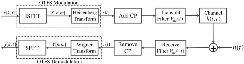
Figure 1: Block diagram of OTFS transmitter (top) and receiver (bottom).

The baseband diagram of OTFS system is given in Fig. 1. Specifically, OTFS modulation starts with a cascade of a pair of 2D transforms at the transmitter. The modulator first maps the information symbols $x[k,\ell]$ in the delay-Doppler domain to $X[n,m]$ in time-frequency plane by using the inverse symplectic finite Fourier transform (ISFFT). Consider the $NM$ data symbols $\left\{{x[k,\ell],k=0,\cdots,N-1;\ell=0,\cdots,M-1}\right\}$ from a modulation alphabet $\mathbb{A}=\left\{{{a_{1}},{a_{2}},\cdots,{a_{Q}}}\right\}$ (e.g., QAM symbols), which are placed on the delay-Doppler plane $\Gamma$. By using the ISFFT, the $NM$ symbols are converted into the time-frequency plane $\Lambda$:

$$X[n,m]=\frac{1}{{\sqrt{NM}}}\sum\limits_{k=0}^{N-1}{\sum\limits_{\ell=0}^{M-1}{x[k,\ell]{e^{j2\pi\left({\frac{{nk}}{N}-\frac{{m\ell}}{M}}\right)}}}},\;n=0,\cdots,N-1;\;m=0,\cdots,M-1.$$ (3)

Next, time-frequency signals $X[n,m]$ are transformed into a time domain signal $s(t)$ through Heisenberg transform utilizing transmit pulse ${g_{tx}}(t)$:

$$s(t)=\sum\limits_{n=0}^{N-1}{\sum\limits_{m=0}^{M-1}{X[n,m]{g_{tx}}(t-nT){e^{j2\pi\left({m{\rm{-}}\frac{{M{\rm{-1}}}}{{\rm{2}}}}\right)\Delta f(t-nT)}}}}.$$ (4)

We apply a CP of length at least equal to the maximum baseband channel delay spread. After inserting a CP in $s(t)$ to tackle inter-frame interference, the time domain signal passes through the transmit filter before entering the (baseband) channel with baseband impulse response

$$h(t,p{T_{s}})=\sum\limits_{i=1}^{L}{{h_{i}}{e^{j2\pi{\nu_{i}}\left({t-p{T_{s}}}\right)}}{{\mathop{\rm P}\nolimits}_{\text{{rc}}}}(p{T_{s}}-{\tau_{i}})},\;p=0,\cdots,P-1,$$ (5)

where $L$ is the number of multipaths and ${T_{s}}={1\mathord{\left/{\vphantom{1{M\Delta f}}}\right.\kern-1.2pt}{M\Delta f}}$ is the SSS interval; ${{h_{i}}}$, ${{\tau_{i}}}$ and ${{\nu_{i}}}$ represent the gain, delay and Doppler shift associated with the $i$-th path, respectively.

Note that ${{{\mathop{\rm P}\nolimits}_{\text{{rc}}}}(p{T_{s}}-{\tau_{i}})}$ represents the sampled equivalent filter response that includes bandlimiting pulse-shaping filters used by both transmitter and receiver to control signal bandwidth and to reject out-of-band interferences. Generally speaking, ${{{\mathop{\rm P}\nolimits}_{\text{{rc}}}}(\tau)}$ is a raised-cosine (RC) rolloff pulse if the transmit filter response is a root raised-cosine (RRC) rolloff pulse and the receive filter is its corresponding matched filter. In addition, we denote the Doppler tap for the $i$-th path as ${\nu_{i}}=({{k_{{\nu_{i}}}}+{\beta_{{\nu_{i}}}}})/NT$, where integer ${{k_{{\nu_{i}}}}}$ represents the index of Doppler frequency ${\nu_{i}}$ and ${\beta_{{\nu_{i}}}}\in\left({-0.5,0.5}\right]$ is the fractional shift of the nearest Doppler tap ${{k_{{\nu_{i}}}}}$. The channel order $P$ is chosen according to the duration of the filter response and the maximum channel delay spread.

At the receiver, the received signal enters a user-defined receive filter before CP removal. The received signal $r(t)$ is given by

$$r(t)=\sum\limits_{p=0}^{P-1}{\sum\limits_{i=1}^{L}{{h_{i}}{e^{j2\pi{\nu_{i}}\left({t-p{T_{s}}}\right)}}{{\mathop{\rm P}\nolimits}_{\text{{rc}}}}(p{T_{s}}-{\tau_{i}})}s(t-p{T_{s}})}+N(t),$$ (6)

where the filtered noise is $N(t)=\int_{\mu}{n(t+\mu){{\mathop{\rm P}\nolimits}_{\text{{rrc}}}}(\mu)d\mu}$. Note that ${{{\mathop{\rm P}\nolimits}_{\text{{rrc}}}}(\mu)}$ is typically an RRC rolloff receive filter and ${n(t)}$ represents the additive white Gaussian noise (AWGN) at the receiver.

The resulting time domain signal $r(t)$ is transformed back to the time-frequency domain through Wigner transform (i.e., inverse of Heisenberg transform). The Wigner transform computes the cross-ambiguity function ${A_{{g_{rx}},r}}(t,f)$ given by

$$Y(t,f)={A_{{g_{rx}},r}}(t,f)\buildrel\Delta\over{=}\int{g_{rx}^{*}(t^{\prime}-t)r(t^{\prime}){e^{-j2\pi f(t^{\prime}-t)}}dt^{\prime}},$$ (7)

and the SSS baseband received signal output is obtained by sampling $Y(t,f)$ as

$$Y[n,m]={\left.{Y(t,f)}\right|_{t=nT,f=\left({m{\rm{-}}\frac{{M{\rm{-1}}}}{{\rm{2}}}}\right)\Delta f}},\;{n=0,\cdots,N-1};\;{m=0,\cdots,M-1}.$$ (8)

Finally, the symplectic finite Fourier transform (SFFT) recovers the delay-Doppler domain data symbol

$$y[k,\ell]=\frac{1}{{\sqrt{NM}}}\sum\limits_{n=0}^{N-1}{\sum\limits_{m=0}^{M-1}{Y[n,m]{e^{-j2\pi\left({\frac{{nk}}{N}-\frac{{m\ell}}{M}}\right)}}}},\;{k=0,\cdots,N-1;\;\ell=0,\cdots,M-1}.$$ (9)

These operations provide the basis of OTFS model with SSS approach in a general case. They are very useful to further study OTFS system when the specific pulses are employed.

For analytical convenience, we capture the relationship between $X[n,m]$ and output $Y[n,m]$ in the following theorem.

Theorem 1.

The input-output relationship of OTFS in time-frequency domain is given by

$$Y[n,m]=\sum\limits_{n^{\prime}=0}^{N-1}{\sum\limits_{m^{\prime}=0}^{M-1}{{H_{n,m}}[n^{\prime},m^{\prime}]X[n^{\prime},m^{\prime}]}}+V[n,m],$$ (10)

where $V[n,m]$ is the noise at the output of the Wigner transform and

$${H_{n,m}}[n^{\prime},m^{\prime}] =\sum\limits_{p=0}^{P-1}{\sum\limits_{i=1}^{L}{{h_{i}}{{\mathop{\rm P}\nolimits}_{\text{{rc}}}}(p{T_{s}}-{\tau_{i}}){A_{{g_{rx}},{g_{tx}}}}\left({(n-n^{\prime})T-p{T_{s}},(m-m^{\prime})\Delta f-{\nu_{i}}}\right)}}$$

$$\quad\times{e^{j\pi\left({M-1}\right)\Delta f(p{T_{s}}-(n-n^{\prime})T)}}{e^{j2\pi m^{\prime}\Delta f((n-n^{\prime})T-p{T_{s}})}}{e^{j2\pi{\nu_{i}}\left({nT-p{T_{s}}}\right)}}.$$ (11)

Proof.

See Appendix A. ∎

We can also characterize the relationship between channel output $y[k,\ell]$ and input $x[k,\ell]$ in the following theorem.

Theorem 2.

The input-output relationship of OTFS in delay-Doppler domain is given by

$$y[k,\ell]=\frac{1}{{NM}}\sum\limits_{k^{\prime}=0}^{N-1}{\sum\limits_{\ell^{\prime}=0}^{M-1}{{h_{k,\ell}}[k^{\prime},\ell^{\prime}]x[k^{\prime},\ell^{\prime}]}}+\upsilon[k,\ell],$$ (12)

where $\upsilon[k,\ell]=\frac{1}{{\sqrt{NM}}}\sum\limits_{n=0}^{N-1}{\sum\limits_{m=0}^{M-1}{V[n,m]{e^{-j2\pi\left({\frac{{nk}}{N}-\frac{{m\ell}}{M}}\right)}}}}$ and

$${h_{k,\ell}}[k^{\prime},\ell^{\prime}]=\sum\limits_{n=0}^{N-1}{\sum\limits_{m=0}^{M-1}{\sum\limits_{n^{\prime}=0}^{N-1}{\sum\limits_{m^{\prime}=0}^{M-1}{{H_{n,m}}[n^{\prime},m^{\prime}]}}{e^{-j2\pi\left({\frac{{nk}}{N}-\frac{{m\ell}}{M}}\right)}}{e^{j2\pi\left({\frac{{n^{\prime}k^{\prime}}}{N}-\frac{{m^{\prime}\ell^{\prime}}}{M}}\right)}}}}.$$ (13)

Proof.

See Appendix B. ∎

In the next section, we will consider a practical communication system, where the rectangular pulses are adopted by both the transmitter and receiver.

III OTFS Model Based on SSS for Rectangular Pulses

Recall that many existing works on OTFS [6, 7, 8, 9, 10, 11, 12, 13, 14, 16, 17, 18, 19, 26, 27] relied on certain impractical assumptions such as ideal bi-orthogonal pulses and on-the-grid delay and/or Doppler shifts. In this section, we first prove that OTFS with rectangular pulses at both transmitter and receiver, the bi-orthogonal condition in (2), can be satisfied. However, for time-varying channels, the ideal bi-orthogonal condition in (17) does not hold. We then derive a general input-output relationship of OTFS system in delay-Doppler domain for SSS.

Let ${\bar{u}}(t)$ denote the unit step function. Without loss of generality, we consider rectangular pulses $\mbox{rect}(t)=T^{-1/2}\cdot[{\bar{u}}(t)-{\bar{u}}(t-T)]$. Given rectangular transmitter and receiver OTFS pulses ${g_{tx}}(t)=g_{rx}(t)=\mbox{rect}(t)$, we have the following result:

Proposition 1.

The rectangular pulses used by both the transmitter and receiver can satisfy the bi-orthogonal condition in (2), i.e.,

$$\int{{e^{-j2\pi m\Delta f(t-nT)}}g_{rx}^{*}(t-nT){g_{tx}}(t)dt}=\delta[m]\delta[n].$$ (14)

Proof.

For $n\neq 0$, we clearly have $\int{{e^{-j2\pi m\Delta f(t-nT)}}g_{rx}^{*}(t-nT){g_{tx}}(t)dt}=0$ due to the finite time duration $T$ of the rectangular pulses $\mbox{rect}(t)$. For $n=0$, we have

$$\int{{e^{-j2\pi m\Delta f(t-nT)}}g_{rx}^{*}(t-nT){g_{tx}}(t)dt}=\frac{1}{T}\int_{0}^{T}{{e^{-j2\pi m\Delta ft}}dt}=\delta[m].$$

The proof is complete by combining both cases. ∎

However, when incorporating time-varying channel (5), rectangular pulses cannot guarantee the following ideal bi-orthogonal condition

$$A_{g_{rx},g_{tx}}(t,f) =\delta[m]\delta[n]q_{(-(P-1){T_{s}},0)}(t)q_{(-\nu_{\max},\nu_{\max})}(f),\begin{array}[]{l}t=\left(nT-(P-1){T_{s}},nT\right),\\ f=(-\nu_{\max}+m\Delta f,\nu_{\max}+m\Delta f),\end{array}$$ (17)

where ${q_{(a,b)}}(x)=1$ for $x\in(a,b)$ and $0$ otherwise. This ideal bi-orthogonal condition in (17) ensures that the ISI is eliminated at the receiver in a practical communication system. However, an ideal pulses which satisfy the above ideal bi-orthogonal condition cannot be realized in practice due to Heisenberg uncertainty principle [21]. Thus, the ISI is inevitable at receiver input such that receiver equalization is necessary for satisfactory reception performance.

Considering the rectangular pulses and the CP effect, we can rewrite ${{H_{n,m}}[n^{\prime},m^{\prime}]}$ in (1) as

$${H_{n,m}}[n^{\prime},m^{\prime}] =\sum\limits_{p=0}^{P-1}{\sum\limits_{i=1}^{L}{{h_{i}}{{\mathop{\rm P}\nolimits}_{\text{{rc}}}}(p{T_{s}}-{\tau_{i}}){A_{{g_{rx}},{g_{tx}}}}\left({{{\left[{n-n^{\prime}}\right]}_{N}}T-p{T_{s}},(m-m^{\prime})\Delta f-{\nu_{i}}}\right)}}$$

$$\quad\times{e^{j\pi\left({M-1}\right)\Delta f\left({p{T_{s}}-{{\left[{n-n^{\prime}}\right]}_{N}}T}\right)}}{e^{j2\pi m^{\prime}\Delta f\left({{{\left[{n-n^{\prime}}\right]}_{N}}T-p{T_{s}}}\right)}}{e^{j2\pi{\nu_{i}}\left({nT-p{T_{s}}}\right)}},$$ (18)

where the cross-ambiguity function ${{A_{{g_{rx}},{g_{tx}}}}\left({{{\left[{n-n^{\prime}}\right]}_{N}}T-p{T_{s}},(m-m^{\prime})\Delta f-{\nu_{i}}}\right)}$ is non-zero for $p=0,\cdots,P-1$ and $\left|{{\nu_{i}}}\right|<{\nu_{\max}}$ only when ${\left[{n-n^{\prime}}\right]_{N}}\leq 1$, i.e., $n^{\prime}=n$ and $n^{\prime}={\left[{n-1}\right]_{N}}$. Hence, the time-frequency relationship in (10) reduces to

$$Y[n,m] ={H_{n,m}}[n,m]X[n,m]+\sum\limits_{m^{\prime}=0,m^{\prime}\neq m}^{M-1}{{H_{n,m}}[n,m^{\prime}]X[n,m^{\prime}]}$$

$$\quad+\sum\limits_{m^{\prime}=0}^{M-1}{{H_{n,m}}\left[{{{\left[{n-1}\right]}_{N}},m^{\prime}}\right]X\left[{{{\left[{n-1}\right]}_{N}},m^{\prime}}\right]}+V[n,m],$$ (19)

in which the first term contains the desired signal, the second and third terms represent ICI and ISI, respectively. The following theorem summarizes the findings:

Theorem 3.

The OTFS input-output relationship in delay-Doppler domain with rectangular pulses is given by

$$y[k,\ell]=\sum\limits_{p=0}^{P-1}{\sum\limits_{i=1}^{L}{\sum\limits_{q=0}^{N-1}{{h_{i}}{{\mathop{\rm P}\nolimits}_{\text{{rc}}}}(p{T_{s}}-{\tau_{i}})\gamma(k,\ell,p,q,{k_{{\nu_{i}}}},{\beta_{{\nu_{i}}}})x\left[{{{\left[{k-{k_{{\nu_{i}}}}+q}\right]}_{N}},{{\left[{\ell-p}\right]}_{M}}}\right]}}}+\upsilon[k,\ell],$$ (20)

where

$$\gamma(k,\ell,p,q,{k_{{\nu_{i}}}},{\beta_{{\nu_{i}}}})=\begin{cases}\frac{1}{N}\xi(\ell,p,{k_{{\nu_{i}}}},{\beta_{{\nu_{i}}}})\theta(q,{\beta_{{\nu_{i}}}}),&p\leq\ell<M,\\ \frac{1}{N}\xi(\ell,p,{k_{{\nu_{i}}}},{\beta_{{\nu_{i}}}})\theta(q,{\beta_{{\nu_{i}}}})\phi(k,q,{k_{{\nu_{i}}}}),&0\leq\ell<p,\end{cases}$$ (21a)

$$\xi(\ell,p,{k_{{\nu_{i}}}},{\beta_{{\nu_{i}}}})={e^{j\pi\frac{{M-1}}{M}p}}{e^{j2\pi\left({\frac{{\ell-p}}{M}}\right)\left({\frac{{{k_{{\nu_{i}}}}+{\beta_{{\nu_{i}}}}}}{N}}\right)}},$$ (21b)

$$\theta(q,{\beta_{{\nu_{i}}}})=\frac{{{e^{-j2\pi(-q-{\beta_{{\nu_{i}}}})}}-1}}{{{e^{-j\frac{{2\pi}}{N}(-q-{\beta_{{\nu_{i}}}})}}-1}},$$ (21c)

$$\phi(k,q,{k_{{\nu_{i}}}})={e^{-j\pi\left({M-1}\right)}}{e^{-j2\pi\frac{{{{\left[{k-{k_{{\nu_{i}}}}+q}\right]}_{N}}}}{N}}}.$$ (21d)

Proof.

See Appendix C. ∎

Note that the magnitude of $\theta(q,{\beta_{{\nu_{i}}}})$ in (21c) peaks at $q=0$ and decreases rapidly as $|q|$ grows. Hence, we can only consider a small number $2{E_{i}}+1$ (${E_{i}}\geq 0$) of significant values $\theta(q,{\beta_{{\nu_{i}}}})$ in (21c), i.e., $-{E_{i}}\leq q\leq{E_{i}}$. By using this approximation, we can conveniently rewrite the received signal $y[k,\ell]$ in (20):

$$y[k,\ell]\approx\sum\limits_{p=0}^{P-1}{\sum\limits_{i=1}^{L}{\sum\limits_{q=-{E_{i}}}^{{E_{i}}}{{h_{i}}{{\mathop{\rm P}\nolimits}_{\text{{rc}}}}(p{T_{s}}-{\tau_{i}})\gamma(k,\ell,p,q,{k_{{\nu_{i}}}},{\beta_{{\nu_{i}}}})x\left[{{{\left[{k-{k_{{\nu_{i}}}}+q}\right]}_{N}},{{\left[{\ell-p}\right]}_{M}}}\right]}}}+\upsilon[k,\ell].$$ (22)

In addition, the relationship of (20) can be simplified as follows if Doppler shifts are exactly on the grid such that ${\beta_{{\nu_{i}}}}{\rm{=0,}}\;\forall i$ without fractional Doppler shift:

Proposition 2.

For Doppler shifts exactly on the grid, the relationship of (20) reduces to

$$y[k,\ell]=\sum\limits_{p=0}^{P-1}{\sum\limits_{i=1}^{L}{{h_{i}}{{\mathop{\rm P}\nolimits}_{rc}}(p{T_{s}}-{\tau_{i}})\gamma(k,\ell,p,{k_{{\nu_{i}}}})x\left[{{{\left[{k-{k_{{\nu_{i}}}}}\right]}_{N}},{{\left[{\ell-p}\right]}_{M}}}\right]}}+\upsilon[k,\ell],$$ (23)

where

$$\gamma(k,\ell,p,{k_{{\nu_{i}}}})=\begin{cases}\xi(\ell,p,{k_{{\nu_{i}}}},0),&p\leq\ell<M,\\ \xi(\ell,p,{k_{{\nu_{i}}}},0){e^{-j\pi\left({M-1}\right)}}{e^{-j2\pi\frac{{{{\left[{k-{k_{{\nu_{i}}}}}\right]}_{N}}}}{N}}},&0\leq\ell<p.\end{cases}$$ (24)

Proof.

The proof follows directly by noting from (21c) that

$$\theta(q,0)=\sum_{n=0}^{N-1}e^{j\frac{2\pi}{N}nq}=\begin{cases}N,&[q]_{N}=0,\\ 0,&\text{otherwise}.\end{cases}=N\delta\left[[q]_{N}\right].$$ (25)

Here we defined $[q]_{N}$ as the remainder of $q$ dividing $N$. Accordingly, the result in (23) follows from (20). ∎

From Theorem 3, we observe that the ISI and extra phase shifts at the receiver can affect the symbol detection when OTFS uses the practical rectangular pulses in Heisenberg and Wigner transforms. Even the simplified model for on-the-grid Doppler shifts in Proposition 2, the ISI is still present. Therefore, simple and effective receiver must be designed to recover the signal in such practical and non-ideal OTFS setups.

IV Receiver Design for OTFS with FSS

Recalling from the literature such as [31, 28] that the use of RRC filter at the transmitter and the matched receive filter would widen the bandwidth beyond the minimum required bandwidth of $1/2T_{s}$. Thus, symbol spaced sampling (SSS), typically, would not preserve sufficient statistic for signal recovery since it falls below Nyquist sampling rate and could also lead to performance sensitivity at the sampling instants [31, 28].

To develop more effective and robust receiver algorithms, we attempted to design a fractionally spaced sampling (FSS) receiver for OTFS with rectangular pulses and RRC filters, which is expected to be able to generate weakly-correlated noises, admit sufficient statistic [31, 28] and further improve the equalization performance. Note that our proposed receivers can be generalized to the non-rectangular pulses in a straightforward manner following the steps from Appendices A, B and C.

IV-A Receiver Structure

When sampling at a rate that is an integer multiple $G$ of the symbol rate, FSS receiver is equivalent to a SIMO linear system in which $G$ multiple parallel channels have correlated noise [28]. The SIMO channel responses depend on the time-varying channel as well as transmit and receive filters. For the receive filter output to be sampled at rate $G/{{T_{s}}}$, we first write its polyphase representation after the removal of the CP as

$${r_{g}}[u]=\sum\limits_{p=0}^{P-1}{\sum\limits_{i=1}^{L}{{h_{i}}{e^{j2\pi{\nu_{i}}\left({uT_{s}-p{T_{s}}}\right)}}{{\mathop{\rm P}\nolimits}_{\text{{rc}}}}[g]}s(uT_{s}-p{T_{s}})}+{N_{g}}[u],\begin{array}[]{l}u=0,\cdots,NM-1,\\ g=0,\cdots,G-1,\end{array}$$ (28)

where the $g$-th channel output sequence is ${r_{g}}[u]\stackrel{{\scriptstyle\triangle}}{{=}}r(uT_{s}+{{g{T_{s}}}\mathord{\left/{\vphantom{{g{T_{s}}}G}}\right.\kern-1.2pt}G})$ with additive noise ${N_{g}}[u]\stackrel{{\scriptstyle\triangle}}{{=}}N(uT_{s}+{{g{T_{s}}}\mathord{\left/{\vphantom{{g{T_{s}}}G}}\right.\kern-1.2pt}G})$, and ${{\rm{P}}_{\text{{rc}}}}[g]\buildrel\Delta\over{=}{{\rm{P}}_{\text{{rc}}}}(p{T_{s}}+{{g{T_{s}}}\mathord{\left/{\vphantom{{g{T_{s}}}G}}\right.\kern-1.2pt}G}-{\tau_{i}})$ for simplicity. The resulting SIMO receiver structure diagram for OTFS system is given in Fig. 2.

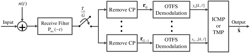
Figure 2: Receiver structure of FSS approach for OTFS system.

To utilize the multiple receptions for diversity combining, we proceed with our FSS-OTFS system model. By performing an OTFS demodulation at the receiver for each $g$, we obtain the following relationship:

$${y_{g}}[k,\ell] =\sum\limits_{p=0}^{P-1}{\sum\limits_{i=1}^{L}{\sum\limits_{q=0}^{N-1}{{h_{i}}{{\mathop{\rm P}\nolimits}_{\text{{rc}}}}[g]\gamma(k,\ell,p,q,{k_{{\nu_{i}}}},{\beta_{{\nu_{i}}}})x\left[{{{\left[{k-{k_{{\nu_{i}}}}+q}\right]}_{N}},{{\left[{\ell-p}\right]}_{M}}}\right]}}}+{\upsilon_{g}}[k,\ell]$$ (29a)

$$\approx\sum\limits_{p=0}^{P-1}{\sum\limits_{i=1}^{L}{\sum\limits_{q=-{E_{i}}}^{{E_{i}}}{{h_{i}}{{\mathop{\rm P}\nolimits}_{\text{{rc}}}}[g]\gamma(k,\ell,p,q,{k_{{\nu_{i}}}},{\beta_{{\nu_{i}}}})x\left[{{{\left[{k-{k_{{\nu_{i}}}}+q}\right]}_{N}},{{\left[{\ell-p}\right]}_{M}}}\right]}}}+{\upsilon_{g}}[k,\ell],$$ (29b)

where ${\upsilon_{g}}[k,\ell]=\frac{1}{{\sqrt{NM}}}\sum\limits_{n=0}^{N-1}{\sum\limits_{m=0}^{M-1}{{V_{g}}[n,m]}}{e^{-j2\pi\left({\frac{{nk}}{N}-\frac{{m\ell}}{M}}\right)}}$ with ${V_{g}}[n,m]=\int g_{rx}^{*}(t^{\prime}-nT){N_{g}}(t^{\prime})$ $\times{e^{-j2\pi\left({m{\rm{-}}\frac{{M{\rm{-1}}}}{{\rm{2}}}}\right)\Delta f(t^{\prime}-nT)}}dt^{\prime}$.

The input-output relationship in (29) can be vectorized as

$${{\bf{y}}_{g}}\simeq{{\bf{H}}_{g}}{\bf{x}}+{{\bf{z}}_{g}},\;g=0,\cdots,G-1,$$ (30)

where ${\bf{x}},{{\bf{y}}_{g}},{{\bf{z}}_{g}}\in{\mathbb{C}^{NM\times 1}}$ and ${{\bf{H}}_{g}}\in{\mathbb{C}^{NM\times NM}}$. Because of the modulo-$N$ and modulo-$M$ operations in (29), the number of non-zero elements in each row and column of ${{\bf{H}}_{g}}$ is identically $D$. Typically, $D$ is much smaller than $NM$, leading to a sparse matrix ${{\bf{H}}_{g}}$.

For the special case of SSS, the receiver is simplified with $G=1$. One can derive an efficient MP algorithm for symbol detection by rounding the delay and/or Doppler shifts to integers on receiver sampling grid [7, 26].

Because the RRC transmit and receive bandlimiting filter has bandwidth between $1/2T_{s}$ and $1/T_{s}$. Therefore, selecting $G=2$ as FSS interval suffices to preserve the sufficient signal statistic. Thus, we shall focus on the use of $G=2$ henceforth. Unlike in [7] and [26], our proposed receivers can potentially exploit channel spectrum diversity gain to substantially improve the performance without relying on multiple antennas and multiple radio frequency (RF) chains. We also drop the impractical assumption that delay/Doppler shifts must be on the grid. Note that extension to larger $G$, when broader bandwidth becomes available, is straightforward since we can always separate $G$ channels into two groups for receiver equalization.

IV-B ICMP Receiver Equalization

In this part, we will introduce the ICMP receiver to take advantage of the SIMO receptions. To this end, we combine the equations from the receptions in (30) as

$${\bf{y}}={\bf{Hx}}+{\bf{z}},$$ (31)

where ${\bf{y}}={[{\bf{y}}_{0}^{T},{\bf{y}}_{1}^{T}]^{T}}$, ${\bf{H}}={[{\bf{H}}_{0}^{T},{\bf{H}}_{1}^{T}]^{T}}$ and ${\bf{z}}={[{\bf{z}}_{0}^{T},{\bf{z}}_{1}^{T}]^{T}}$. The basic problem now is to detect the transmitted symbol vector ${\bf{x}}$ from the received signals with channel knowledge at the receiver. Direct solution of (31) could be computationally demanding as it involves inversion of a large matrix as $NM$ can typically be in the order of thousands.

Let $\mathcal{I}(d)$ and $\mathcal{J}(c)$ denote the sets of indexes with non-zero elements in the $d$-th row and $c$-th column of ${\bf{H}}$, where $d=1,\cdots,2NM$ and $c=1,\cdots,NM$, respectively. Here, we can interpret the system model in (31) as a sparsely-connected factor graph. Thus, we can apply the concept of low-complexity MP algorithm for symbol detection. Specifically, each entry of the observation vector ${\bf{y}}$ denotes an observation node, whereas each transmitted symbol is viewed as a variable node. In this factor graph, each observation node $y[d]$ is connected to the set of $D$ variable nodes $\{x[c],c\in\mathcal{I}(d)\}$ whereas each variable node $x[c]$ is connected to the set of $2D$ observation nodes $\{y[d],d\in\mathcal{J}(c)\}$.

The optimal way of detecting the transmitted symbols is joint maximum a posterior probability (MAP) detection, i.e.,

$$\mathbf{\hat{x}}=\operatorname*{arg\,max}_{\mathbf{x}\in\mathbb{A}^{NM\times 1}}\Pr\bigl{(}\mathbf{x|y,H}\bigr{)},$$

which has a complexity exponential in $NM$. This can be intractable when the product $NM$ is in the order of several thousands. As a result, we derive a suboptimal symbol-by-symbol MAP detection through following approximation:

$$\hat{x}[c] =\operatorname*{arg\,max}_{a_{j}\in\mathbb{A}}\Pr\bigl{(}x[c]=a_{j}|\mathbf{y,H}\bigr{)}$$

$$=\operatorname*{arg\,max}_{a_{j}\in\mathbb{A}}\Pr(x[c]={a_{j}})\Pr\bigl{(}\mathbf{y}|x[c]=a_{j},\mathbf{H}\bigr{)}$$

$$\approx\operatorname*{arg\,max}_{a_{j}\in\mathbb{A}}{\omega_{c}}({a_{j}})\prod_{d\in\mathcal{J}(c)}{\Pr(y[d]\left|{x[c]={a_{j}},{\bf{H}}}\right.)}$$ (32)

In (32), we denote a priori probability when $x[c]=a_{j}$ as ${\omega_{c}}({a_{j}})$ and assume the components of $\mathbf{y}$ are approximately independent for a given $x[c]$ due to the sparsity of $\mathbf{H}$. To further reduce complexity, we employ the Gaussian approximation of the interference components within the proposed ICMP receiver. Similar to [7, 26], this algorithm performs message passing iteratively among observation nodes and variable nodes according to the factor graph. The ICMP receiver is summarized in Algorithm 1. Below are its detailed steps in iteration $\kappa$:

Algorithm 1 ICMP Receiver

  Input: ${\bf{y}}$, ${\bf{H}}$, ${\omega_{c}}({a_{j}})={1\mathord{\left/{\vphantom{1Q}}\right.\kern-1.2pt}Q}$, $c=1,\cdots NM$, $j=1,\cdots Q$ and $n_{iter}$.

  Initialization: ${\bf{p}}_{c,d}^{(0)}={{\bm{\omega}}_{c}}$, $c=1,\cdots NM$, $d\in\mathcal{J}(c)$, $\eta^{(0)}=0$ and iteration count $\kappa=1$.

  repeat

     

1. Each observation node $y[d]$ computes the mean $\mu_{d,c}^{(\kappa)}$ and variance ${{(\sigma_{d,c}^{(\kappa)})}^{2}}$ in (34) and (35), then passes them to the connected variable nodes $x[c],c\in\mathcal{I}(d)$;

2. Each variable node $x[c]$ generates ${\bf{p}}_{c,d}^{(\kappa)}$ in (36) and passes them to the connected observation nodes $y[d],d\in\mathcal{J}(c)$;

3. Compute the convergence indicator $\eta^{(\kappa)}$ and symbol probabilities ${\bf{p}}_{c}^{(\kappa)}$ in (37);

4. Update decision symbol probabilities ${\bf{\bar{p}}}_{c}={\bf{p}}_{c}^{(\kappa)}$ if $\eta^{(\kappa)}>\eta^{(\kappa-1)}$;

5. $\kappa:=\kappa+1$;

  until $\eta^{(\kappa)}=1$ or $\kappa=n_{iter}$.

  Output: The decisions of the transmitted symbols in (39).

From observation node $y[d]$ to variable nodes $x[c],c\in\mathcal{I}(d)$: At each observation node, extrinsic messages to each connected variable node is computed according to the channel model, noisy channel observations, and a priori information from other connected variable nodes. The received signal $y[d]$ can be written as

$$y[d]=H[d,c]x[c]+\underbrace{\sum\limits_{e\in{\cal I}(d),e\neq c}H[d,e]x[e]+z[d]}_{\zeta_{d,c}^{(\kappa)}},$$ (33)

where sum of interference and noise $\zeta_{d,c}^{(\kappa)}$ is approximately modeled as $\mathcal{CN}\left({\mu_{d,c}^{(\kappa)},{{(\sigma_{d,c}^{(\kappa)})}^{2}}}\right)$ according to Central Limit Theorem [32], with

$$\mu_{d,c}^{(\kappa)}=\sum_{e\in\mathcal{I}(d),e\neq c}\sum_{j=1}^{Q}p_{e,d}^{(\kappa-1)}(a_{j})a_{j}H[d,e],$$ (34)

$${(\sigma_{d,c}^{(\kappa)})^{2}}=\sum\limits_{e\in{\cal I}(d),e\neq c}{\left({\sum\limits_{j=1}^{Q}{p_{e,d}^{(\kappa-1)}}({a_{j}}){{\left|{{a_{j}}}\right|}^{\rm{2}}}{{\left|{H[d,e]}\right|}^{\rm{2}}}-{{\left|{\sum\limits_{j=1}^{Q}{p_{e,d}^{(\kappa-1)}}({a_{j}}){a_{j}}H[d,e]}\right|}^{\rm{2}}}}\right)}+\sigma_{N}^{2}.$$ (35)

In (35), $\sigma_{N}^{2}=\sigma_{n}^{2}\int_{\mu}{{\mathop{\rm P}\nolimits}_{\text{{rrc}}}^{2}(\mu)d\mu}$ is the variance of the colored Gaussian noise after the receive filter and $\sigma_{n}^{2}$ is the variance of the AWGN $\bf{n}$ at the receiver input. The mean $\mu_{d,c}^{(\kappa)}$ and variance ${{(\sigma_{d,c}^{(\kappa)})}^{2}}$ are used as messages passed from observation nodes to variable nodes.

From variable node $x[c]$ to observation nodes $y[d],d\in\mathcal{J}(c)$: At each variable node, the extrinsic information for each connected observation node is generated from prior messages collected from other observation nodes. A posteriori log-likelihood ratio (LLR) is given by

$$\alpha_{c}^{(\kappa)}({a_{j}}) =\log\frac{{{\omega_{c}}({a_{j}})\prod\limits_{e\in{\cal J}(c)}{\Pr(y[e]\left|{x[c]={a_{j}},{\bf{H}}}\right.)}}}{{{\omega_{c}}({a_{Q}})\prod\limits_{e\in{\cal J}(c)}{\Pr(y[e]\left|{x[c]={a_{Q}},{\bf{H}}}\right.)}}}$$

$$=\underbrace{\log\frac{{{\omega_{c}}({a_{j}})\prod\limits_{e\in{\cal J}(c),e\neq d}{\Pr(y[e]\left|{x[c]={a_{j}},{\bf{H}}}\right.)}}}{{{\omega_{c}}({a_{Q}})\prod\limits_{e\in{\cal J}(c),e\neq d}{\Pr(y[e]\left|{x[c]={a_{Q}},{\bf{H}}}\right.)}}}}_{\alpha_{c,d}^{(\kappa)}({a_{j}})}+\underbrace{\log\frac{{\Pr(y[d]\left|{x[c]={a_{j}},{\bf{H}}}\right.)}}{{\Pr(y[d]\left|{x[c]={a_{Q}},{\bf{H}}}\right.)}}}_{\Lambda_{c,d}^{(\kappa)}({a_{j}})},$$

where $\Lambda_{c,d}^{(\kappa)}({a_{j}})=\log\frac{{\varepsilon_{d,c}^{(\kappa)}({a_{j}})}}{{\varepsilon_{d,c}^{(\kappa)}({a_{Q}})}}$, the extrinsic LLR $\alpha_{c,d}^{(\kappa)}({a_{j}})=\log\frac{{{\omega_{c}}({a_{j}})}}{{{\omega_{c}}({a_{Q}})}}+\sum\limits_{e\in{\cal J}(c),e\neq d}{\log\frac{{\varepsilon_{e,c}^{(\kappa)}({a_{j}})}}{{\varepsilon_{e,c}^{(\kappa)}({a_{Q}})}}}$ and $\varepsilon_{e,c}^{(\kappa)}({a_{j}})=\exp\left({-\frac{{{{\left|{y[e]-\mu_{e,c}^{(\kappa)}-{H_{e,c}}{a_{j}}}\right|}^{2}}}}{{{{(\sigma_{e,c}^{(\kappa)})}^{2}}}}}\right)$. The message passed from a variable node $x[c]$ to observation nodes $y[d],d\in\mathcal{J}(c)$ is the probability mass function of the alphabet

$$p_{c,d}^{(\kappa)}(a_{j})=\Delta\cdot\tilde{P}_{c,d}^{(\kappa)}(a_{j})+(1-\Delta)\cdot p_{c,d}^{(\kappa-1)}(a_{j}),\ a_{j}\in\mathbb{A},$$ (36)

where $\tilde{P}_{c,d}^{(\kappa)}({a_{j}}){\rm{}}=\left[\sum\limits_{k=1}^{Q}{\exp\left({\alpha_{c,d}^{(\kappa)}({a_{k}})}\right)}\right]^{-1}{\exp\left({\alpha_{c,d}^{(\kappa)}({a_{j}})}\right)}$ and $\Delta\in(0,1]$ is a message damping factor used to improve performance by controlling convergence speed [33, 7, 26].

Convergence indicator: The convergence indicator $\eta^{(\kappa)}$ can be computed as

$$\eta^{(\kappa)}=\frac{1}{NM}\sum_{c=1}^{NM}\mathbb{I}\Biggl{(}\max_{a_{j}\in\mathbb{A}}\ p_{c}^{(\kappa)}(a_{j})\geq 1-\varrho\Biggr{)}$$ (37)

for some small $\varrho>0$ and where $p_{c}^{(\kappa)}({a_{j}})=\left[{\sum\limits_{k=1}^{Q}{\exp\left({\alpha_{c}^{(\kappa)}({a_{k}})}\right)}}\right]^{-1}{{\exp\left({\alpha_{c}^{(\kappa)}({a_{j}})}\right)}}$. $\mathbb{I}(\cdot)$ denotes the indicator function.

Update criteria: If $\eta^{(\kappa)}>\eta^{(\kappa-1)}$, then we update the probabilities of transmitted symbols as

$${\bf{\bar{p}}}_{c}={\bf{p}}_{c}^{(\kappa)},\ c=1,\dots,NM.$$ (38)

Note that we only update the probabilities if the current iteration is better than the previous one.

Stopping criteria: The MP algorithm stops if either $\eta^{(\kappa)}=1$ or the maximum number of iterations $n_{iter}$ is reached.

Once the stopping criteria is satisfied, we make the decisions of the transmitted symbols as

$$\hat{x}[c]=\operatorname*{arg\,max}_{a_{j}\in\mathbb{A}}\bar{p}_{c}({a_{j}}),\ c=1,\dots,NM.$$ (39)

Even though ICMP receiver can exploit the SIMO channel diversity gain, the performance may degenerate when the corresponding jointly factor graph of the parallel correlated channels is densely connected to form short cycles [34]. Unfortunately, OTFS often exhibits a high density graph due to off-grid channel delays and Doppler shifts. In addition, the performance can also suffer when Gaussian approximation of the interference terms becomes less accurate. To overcome these shortcomings, we propose a more efficient TMP receiver in the next subsection.

IV-C TMP Receiver Equalization

Since there are two receive channels from (30), an MP equalizer can be applied for each reception typically. Given two MP equalizers, we propose a turbo receiver to enable cooperation between these two MP equalizers for better performance. In the TMP receiver, two individual MP equalizers exchange information in the form of LLRs for each symbol. The extrinsic LLRs generated by one MP equalizer are treated as a priori information by the other. As soft information is circulated via this algorithmic loop, more reliable soft information produced in one equalizer helps the other to improve. Improved bit error rate (BER) performance can be achieved as iterations continues and are terminated after a certain number $n_{t}$ of iterations.

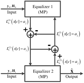
Figure 3: TMP receiver structure.

The TMP receiver structure is shown in Fig. 3. A similar MP algorithm as in Algorithm 1 can be employed for each equalizer with only modest modifications of input ${{\bm{\omega}}_{c}}$ by a priori information and output the a posteriori information.

Specifically, the first equalizer produces output a posteriori LLR on each symbol as

$$L_{o}^{(1)}\left({x[c]={a_{j}}}\right)=\underbrace{\log\frac{{\Pr({\bf{y}}|x[c]={a_{j}},{\bf{H}})}}{{\Pr({\bf{y}}|x[c]={a_{Q}},{\bf{H}})}}}_{L_{e}^{(1)}\left({x[c]={a_{j}}}\right)}+\underbrace{\log\frac{{\Pr(x[c]={a_{j}})}}{{\Pr(x[c]={a_{Q}})}}}_{L_{i}^{(1)}\left({x[c]={a_{j}}}\right)},$$ (40)

where $c=1,\cdots,NM$ and $j=1,\cdots,Q$. The extrinsic LLR ${L_{e}^{(1)}\left({x[c]={a_{j}}}\right)}$ is then passed to the second equalizer as a priori LLR, i.e., $L_{i}^{(2)}\left({x[c]={a_{j}}}\right)=L_{e}^{(1)}\left({x[c]={a_{j}}}\right)$. Similarly, the second equalizer generate extrinsic LLR $L_{e}^{(2)}\left({x[c]={a_{j}}}\right)=L_{o}^{(2)}\left({x[c]={a_{j}}}\right)-L_{i}^{(2)}\left({x[c]={a_{j}}}\right)$, which is passed back to the first equalizer as a priori information to form the iterative loop. Note that we only pass extrinsic information. Otherwise, messages become more and more correlated over the iterations and the efficiency of the iterative algorithm would be reduced, which results in performance loss [35].

IV-D Performance Analysis of TMP Receiver

Since our proposed FSS receiver can typically generate weakly-correlated channel outputs, the EXIT chart [36, 37] still offers substantially clear insight into the convergence behavior of our proposed TMP receiver. It has been successfully used for analyzing and predicting convergence behavior of iteratively decoded systems [36, 37]. In this subsection, we analyze the performance of the proposed TMP receiver by using the tool of EXIT chart [36, 37], which tracks the evolution of mutual information (MI) between transmitted symbols and their LLRs through iterations. For the EXIT chart of TMP receiver analysis, the two MP equalizers are modeled as the MI transfer devices, i.e., given a priori MI $I_{i}$ at the input, each equalizer generates a new extrinsic MI $I_{e}$ at the output, where ${I_{i}}\buildrel\Delta\over{=}I({{\bf{L}}_{i}};x)$ and ${I_{e}}\buildrel\Delta\over{=}I({{\bf{L}}_{e}};x)$, respectively.

We consider quadrature phase shift keying (QPSK) with Gray mapping as an example, i.e., $\mathbb{A}=\left[{\frac{{1+j}}{{\sqrt{2}}},\frac{{1-j}}{{\sqrt{2}}},\frac{{-1+j}}{{\sqrt{2}}},\frac{{-1-j}}{{\sqrt{2}}}}\right]$ and similar analysis could be done with other modulations. A Gray-mapped QPSK can be regarded as a superposition of the BPSK modulated in-phase and quadrature components, so the MI ${I_{i}}=I_{i}^{(\text{I})}+I_{i}^{(\text{Q})}$ with

$$I_{i}^{(\text{S})}=\frac{1}{2}\sum\limits_{{x^{(\text{S})}}\in\left\{{{1\mathord{\left/{\vphantom{1{\sqrt{2}}}}\right.\kern-1.2pt}{\sqrt{2}}},-{1\mathord{\left/{\vphantom{1{\sqrt{2}}}}\right.\kern-1.2pt}{\sqrt{2}}}}\right\}}{\int_{-\infty}^{\infty}{{f_{L_{i}^{(\text{S})}}}({l^{(\text{S})}}\left|{{x^{(\text{S})}}}\right.){{\log}_{2}}\frac{{2{f_{L_{i}^{(\text{S})}}}({l^{(\text{S})}}\left|{{x^{(\text{S})}}}\right.)}}{{{f_{L_{i}^{(\text{S})}}}({l^{(\text{S})}}\left|{{1\mathord{\left/{\vphantom{1{\sqrt{2}}}}\right.\kern-1.2pt}{\sqrt{2}}}}\right.)+{f_{L_{i}^{(\text{S})}}}({l^{(\text{S})}}\left|{-{1\mathord{\left/{\vphantom{1{\sqrt{2}}}}\right.\kern-1.2pt}{\sqrt{2}}}}\right.)}}d{l^{(\text{S})}}}},$$ (41)

where $\text{S}\in\{\text{I},\text{Q}\}$ and ${{f_{L_{i}^{(\text{S})}}}({l^{(\text{S})}}\left|{{x^{(\text{S})}}}\right.)}$ is the conditional distribution of a priori LLR ${L_{i}^{(\text{S})}}$ given ${x^{(\text{S})}}\in\left\{{\frac{1}{{\sqrt{2}}},-\frac{1}{{\sqrt{2}}}}\right\}$. When the Gaussian approximation is applied to ${{f_{L_{i}^{(\text{S})}}}({l^{(\text{S})}}\left|{{x^{(\text{S})}}}\right.)}$, i.e.,

$${f_{L_{i}^{(\text{S})}}}({l^{(\text{S})}}\left|{{x^{(\text{S})}}}\right.)=\frac{1}{{\sqrt{2\pi}{\sigma_{L_{i}^{(\text{S})}}}}}\exp\left({-\frac{{{{\left({l^{(\text{S})}}-\sqrt{2}\sigma_{L_{i}^{(\text{S})}}^{2}{x^{(\text{S})}}\right)}^{2}}}}{{2\sigma_{L_{i}^{(\text{S})}}^{2}}}}\right),$$ (42)

where ${\sigma_{L_{i}^{(\text{S})}}^{2}}$ is the variance of the LLR random variables $L_{i}^{(\text{S})}$. The MI ${I_{i}}$ can be expressed as

$${I_{i}}({\sigma_{L_{i}^{(\text{S})}}}) =2-2\int_{-\infty}^{\infty}{{f_{L_{i}^{(\text{S})}}}\left({l^{(\text{S})}}\left|{{1\mathord{\left/{\vphantom{1{\sqrt{2}}}}\right.\kern-1.2pt}{\sqrt{2}}}}\right.\right){{\log}_{2}}\left(1+{e^{-2{l^{(\text{S})}}}}\right)d{l^{(\text{S})}}}$$

$$=2-2{E_{{x^{(\text{S})}}={1\mathord{\left/{\vphantom{1{\sqrt{2}}}}\right.\kern-1.2pt}{\sqrt{2}}}}}\left[{\log_{2}}\left(1+{e^{-2L_{i}^{(\text{S})}}}\right)\right],$$ (43)

where ${E_{x}}[\bullet]$ is the expectation value of $x$. Note that the function ${I_{i}}({\sigma_{L_{i}^{(\text{S})}}})$ is monotonically increasing and has an inverse. Additionally, ${\lim_{{\sigma_{L_{i}^{(\text{S})}}}\to 0}}{I_{i}}({\sigma_{L_{i}^{(\text{S})}}})=0$ and ${\lim_{{\sigma_{L_{i}^{(\text{S})}}}\to\infty}}{I_{i}}({\sigma_{L_{i}^{(\text{S})}}})=2$, which correspond to zero and perfect a priori information, respectively.

After passing samples of ${{\bf{L}}_{i}}$ through the MP equalizer, the output of extrinsic MI $I_{e}$ is obtained by applying the same expression in (41) with the distribution of ${{\bf{L}}_{e}}$. This can be achieved by first estimating the conditional distribution of ${{f_{L_{e}^{(\text{S})}}}({l^{(\text{S})}}\left|{{x^{(\text{S})}}}\right.)}$ using the histogram method [36, 37] before computing ${I_{e}}=I_{e}^{(\text{I})}+I_{e}^{(\text{Q})}$ numerically based on (41). The EXIT chart is depicted by repeating the procedure above for several values of ${\sigma_{L_{i}^{(\text{S})}}}$ to yield pairs of $({I_{i}},{I_{e}})$.

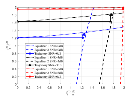
Figure 4: EXIT charts and simulated traces of TMP receiver for QPSK with SNR = 0dB, 3dB and 6dB.

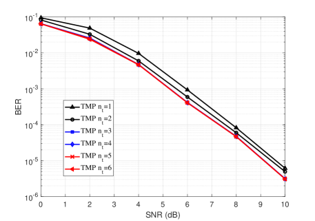
Figure 5: BER performance of TMP receiver with different number of iterations for OTFS system.

Fig. 5 shows an example of the proposed TMP receiver’s EXIT charts for QPSK at different signal-to-noise ratio (SNR) levels. Here we select a typical urban channel model [38] and generate the Doppler shift for each delay by using the Jakes formulation [8, 17, 26] with maximum Doppler frequency shift ${{\nu_{max}}}=1111$ Hz. We observe that the MI ${I_{e}}$ increases with ${I_{i}}$, which means that the output ${{\bf{L}}_{e}}$ becomes more reliable as the input ${{\bf{L}}_{i}}$ becomes better. We also show the trajectories of iterative process of the TMP receiver in Fig. 5. Note that the system trajectories closely follow the transfer curves of the two MP equalizers and eventually reach the corresponding convergence point (where the transfer curves inter-set) for different SNRs. The convergence point becomes more reliable as SNR grows, even approaching the ideal mutual information of 2 bits per QPSK symbol.

The slight discrepancy between trajectories and transfer curves can be attributed to the Gaussian model approximation of the conditional distribution ${{f_{L_{i}^{(\text{S})}}}({l^{(\text{S})}}\left|{{x^{(\text{S})}}}\right.)}$. In addition, we can estimate the number of required iterations for the proposed TMP receiver to converge by counting the number of staircase steps that follow the trajectory curves of Fig. 5. As we can see, three iterations are typically sufficient to achieve the desired performance. This analysis is also verified in Fig. 5, where the performance improvement becomes negligible beyond three iterations.

V Reduced Complexity Receivers

From the algorithm discussion, the complexity of the proposed receivers can be attributed to the MP algorithm. Clearly, for each main loop iteration of the MP algorithm, the number of complex multiplications (CMs) required in steps (34), (35) and (36) are $2MNGDQ$, $MNGD(4Q+1)$ and $5MNGDQ$, respectively. Therefore, the overall computational complexity required respectively for ICMP and TMP receivers are $n_{iter}MNGD(11Q+1)$ and $n_{t}n_{iter}MNGD(11Q+1)$.

We note that the proposed receiver complexity depends critically on the number of non-zero channel ISI terms (i.e., $D$) which represent channel sparsity. However, $D$ can sometimes remain relatively large, e.g. over 150 in our experiments because of many off-grid delays and Doppler shifts. Thus, to further reduce receiver complexity, we propose a simplified MP algorithm by trimming of some graph edges from participating in message passing and update. Although such approximation may lead to some performance loss, edge trimming can also reduce the number of short cycles in the corresponding factor graph, which may in fact improve the performance.

The basic idea is to apply Gaussian approximation to part of the channel interferers (i.e., part of the connections), such that the factor graph can be simplified by trimming these edges. Specifically, for each observation node $y[d]$, we would sort the corresponding $D$ channel coefficients based on their sizes. We choose $R$ largest terms and the corresponding edges to remain in the graph while removing the rest.

Through this process, the received signal $y[d]$ in (33) can be rewritten as

$$y[d]=\sum\limits_{e\in\Phi(d)}H[d,e]x[e]+\underbrace{\sum\limits_{e\in\bar{\Phi}(d)}H[d,e]x[e]+z[d]}_{z^{\prime}[d]},$$ (44)

where ${\Phi(d)}$ represents the set of indices with $R$ largest terms in ${{\cal I}(d)}$ and ${\bar{\Phi}(d)}$ denotes the set containing the indices for the remaining $(D-R)$ terms. We use ${z^{\prime}[d]}$ to denote the new noise term to be approximated as a Gaussian random variable with mean and variance:

$${\mu_{z^{\prime}}}[d]=\sum\limits_{e\in\bar{\Phi}(d)}{\sum\limits_{j=1}^{Q}{{\omega_{e}}}}({a_{j}}){a_{j}}H[d,e],$$ (45)

$${({\sigma_{z^{\prime}}}[d])^{2}}=\sum\limits_{e\in\bar{\Phi}(d)}{\left({\sum\limits_{j=1}^{Q}{{\omega_{e}}}({a_{j}}){{\left|{{a_{j}}}\right|}^{\rm{2}}}{{\left|{H[d,e]}\right|}^{\rm{2}}}-{{\left|{\sum\limits_{j=1}^{Q}{{\omega_{e}}}({a_{j}}){a_{j}}H[d,e]}\right|}^{\rm{2}}}}\right)}+\sigma_{N}^{2}.$$ (46)

Therefore, the messages $\mu_{d,c}^{(\kappa)}$ and ${{(\sigma_{d,c}^{(\kappa)})}^{2}}$ passed from observation node $y[d]$ to variable nodes $x[c],c\in{\Phi(d)}$ in the $\kappa$-th iteration can be expressed as

$$\mu_{d,c}^{(\kappa)}=\sum\limits_{e\in\Phi(d),e\neq c}{\sum\limits_{j=1}^{Q}{p_{e,d}^{(\kappa-1)}}}({a_{j}}){a_{j}}H[d,e]+{\mu_{z^{\prime}}}[d],$$ (47)

$${(\sigma_{d,c}^{(\kappa)})^{2}}=\sum\limits_{e\in\Phi(d),e\neq c}{\left({\sum\limits_{j=1}^{Q}{p_{e,d}^{(\kappa-1)}}({a_{j}}){{\left|{{a_{j}}}\right|}^{\rm{2}}}{{\left|{H[d,e]}\right|}^{\rm{2}}}-{{\left|{\sum\limits_{j=1}^{Q}{p_{e,d}^{(\kappa-1)}}({a_{j}}){a_{j}}H[d,e]}\right|}^{\rm{2}}}}\right)}+{({\sigma_{z^{\prime}}}[d])^{2}}.$$ (48)

Similarly, the message passed from variable node $x[c]$ to observation nodes $y[d],d\in\Psi(c)$ in the $\kappa$-th iteration can still be given in (36) with only modification of $\alpha_{c,d}^{(\kappa)}({a_{j}})$ as

$$\alpha_{c,d}^{(\kappa)}({a_{j}})=\log\frac{{{\omega_{c}}({a_{j}})}}{{{\omega_{c}}({a_{Q}})}}+\sum\limits_{e\in\Psi(c),e\neq d}{\log\frac{{\varepsilon_{e,c}^{(\kappa)}({a_{j}})}}{{\varepsilon_{e,c}^{(\kappa)}({a_{Q}})}}},$$ (49)

where $\Psi(c)$ includes the indices of all the observation nodes that are connected to the variable node $x[c]$ in the simplified factor graph.

As we can see, all the edges participate in message updates in the original MP algorithm whereas the proposed algorithm of simplified MP only retains a subset of edges. Consequently, the overall complexity is reduced to $n_{iter}MNGR(11Q+1)$ and $n_{t}n_{iter}MNGR(11Q+1)$ for simplified ICMP (S-ICMP) receiver and simplified TMP (S-TMP) receiver, respectively.

VI Simulation Results

In this section, we test the performance of our proposed FSS receivers for OTFS systems in high-mobility time-varying channels. For simplicity, we consider that the carrier frequency is $4$ GHz with typical subcarrier spacing ${\Delta f}=15$ kHz. Unless otherwise stated, Gray-mapped QPSK is the modulation and the RRC rolloff factor in transmitter and receiver is set to $0.4$. In addition, we consider $N=32$ time slots and $M=128$ subcarriers in the time-frequency domain. The speed of the mobile user is set to $\lambda=300$ km/h, leading to a maximum Doppler frequency shift ${{\nu_{max}}}=1111$ Hz. We adopt a typical urban channel model [38] with exponentially decaying power delay profile $p(\tau)={e^{-\tau}}$ ($\tau$ is in $\mu$s) and generate the Doppler shift for each delay by using the Jakes formulation [8, 17, 26], i.e., ${\nu_{i}}={\nu_{max}}\cos({\rho_{i}})$, where ${\rho_{i}}$ is uniformly distributed over $[-\pi,\pi]$.

We first assume that the CSI is known at the receiver. We then investigate the effect of imperfect CSI on OTFS performance. Without loss of generality, we choose $\Delta=0.7$, $\varrho=0.1$ and $n_{iter}=20$ for Algorithm 1 and set $G=2$, $n_{t}=3$. All simulation results are from averaging results over 500 realizations.

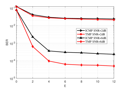
Figure 6: BER performance of OTFS for different numbers of $E$.

We first study the effects of approximation $E_{i}$ on OTFS performance. For simplicity, we consider the same $E_{i}$ for all paths, i.e., ${E_{i}}=E,\forall i$. Fig. 6 illustrates the BER performance of OTFS system versus different numbers of $E$ for different receivers under various levels of SNR (signal quality). We can see significant performance improvement when $E$ increases from $0$ to $6$ at the expense of higher complexity. We also notice a performance saturation thereafter for both receivers, indicating that, because of many small ISI channel taps for off-grid delays and Doppler shifts, very large choices of $E$ do not noticeably improve receiver performance. In the rest of our experiments, we shall use $E=6$ unless otherwise noted.

Fig. 7 compares the BER performance of OTFS system for different receiver designs. To highlight the superiority of the proposed FSS architecture, we also provide the benchmark performance of traditional SSS receiver by limiting on-the-grid delay/Doppler shifts in Fig. 7. The results reveal that every receiver benefits from higher SNR. However, our proposed FSS receivers outperform SSS receivers significantly owing to the utilization of channel diversity gain through fractionally spaced sampling. We also note that the modest BER performance difference between on-the-grid and off-grid delay/Doppler shifts. This strongly support the robustness and the practicality of our proposed receivers given their ability to tackle any values of delay and Doppler shift.

In general, our proposed TMP receiver achieves superior performance to ICMP receiver through turbo iterations. This performance advantage stems from the fact that ICMP receiver suffers from a large number of short cycles in the channel factor graph and is more prone to convergence to local optimum.

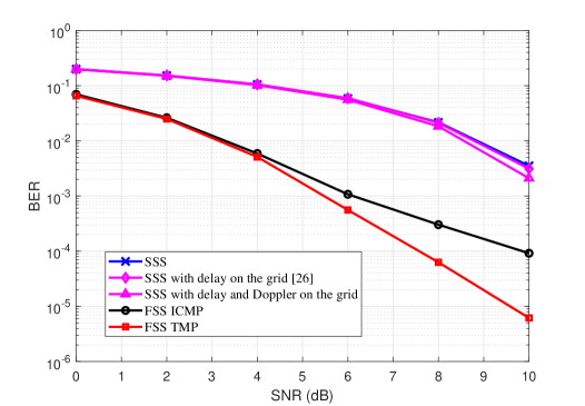
Figure 7: BER performance comparison of OTFS with different receiver designs.

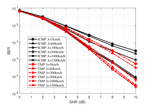
Figure 8: BER performance of OTFS with different user mobile velocities.

Fig. 8 shows the BER performance of OTFS system under various user mobile velocities (i.e., various maximum Doppler shifts). The results show that the performance improves gradually as the user velocity increases from 5 km/h to 500 km/h and saturates beyond 500 km/h. This result would have been surprising to traditional modulation schemes and equalizers that require quasi-static channels. In OTFS, however, the modulation in the delay-Doppler domain in fact can benefit from larger Doppler shift as a larger number of multiple paths becomes more distinct. Our OTFS receiver can resolve a larger number of paths in the Doppler dimension with the help of higher user velocity. As a result, better diversity gain becomes possible.

We again notice that the proposed TMP receiver outperforms ICMP receiver for different velocities, which further exhibits the advantage of TMP receiver over the ICMP receiver for high mobility users.

Fig. 9 shows the BER performance of OTFS transmission with different system parameters. We can observe that the performance of ICMP and TMP receivers degrades as $M$ and $N$ decrease due to the lower resolution of delay-Doppler grid. This leads to the diversity loss since the receiver resolves a smaller number of paths in the channel. We also notice that our FSS receiver can exhibit a certain level of gains even for the high order of modulation (e.g., 16QAM). These analyses strongly support the consistency of our proposed receivers across different system parameters.

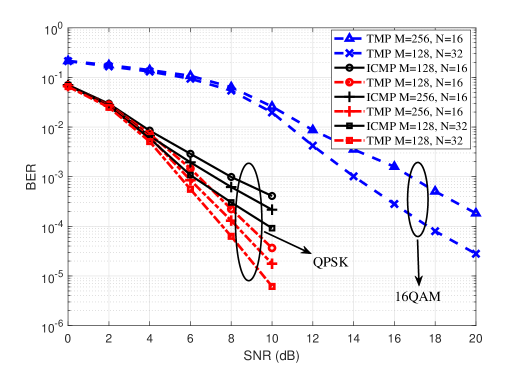
Figure 9: BER performance of OTFS with different system parameters.

For low complexity, Fig. 11 shows the BER performance of OTFS system with the proposed simplified MP receivers. The results clearly show that as $R$ increases, the performance of S-ICMP receiver and S-TMP receiver would approach the performance of ICMP receiver and TMP receiver, respectively. It is worth noting that even with $R=50$, we already achieve a complexity reduction by the factor of around 3 since $D$ is around 150 in our simulation. We further note that the performance loss for the simplified receivers are rather insignificant even if we select smaller $R$. Therefore, our proposed simplified MP receivers can provide the desirable trade-off between complexity and performance.

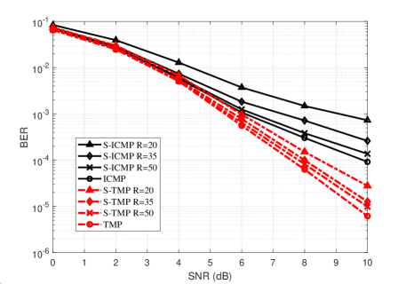
Figure 10: BER performance of OTFS with simplified MP receivers.

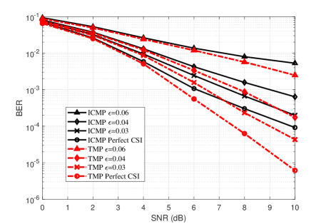
Figure 11: BER performance of OTFS with imperfect CSI.

Finally, we test the effect of CSI uncertainty on the BER performance of OTFS system in Fig. 11. In practice, the receiver can only acquire CSI based on pilots and training which consume power and spectrum resources. It is therefore common that receivers must function under CSI uncertainty. We characterize the CSI error by adopting the following model [39]:

$${h_{i}} ={{\hat{h}}_{i}}+\Delta{h_{i}},\ \left\|{\Delta{h_{i}}}\right\|\leq{\epsilon_{{h_{i}}}},$$

$${\tau_{i}} ={{\hat{\tau}}_{i}}+\Delta{\tau_{i}},\ \left\|{\Delta{\tau_{i}}}\right\|\leq{\epsilon_{{\tau_{i}}}},$$

$${\nu_{i}} ={{\hat{\nu}}_{i}}+\Delta{\nu_{i}},\ \left\|{\Delta{\nu_{i}}}\right\|\leq{\epsilon_{{\nu_{i}}}},$$

where ${{\hat{h}}_{i}}$, ${{\hat{\tau}}_{i}}$ and ${{\hat{\nu}}_{i}}$ are the estimated versions of ${h_{i}}$, ${\tau_{i}}$ and ${\nu_{i}}$. $\Delta{h_{i}}$, $\Delta{\tau_{i}}$ and $\Delta{\nu_{i}}$ represent the corresponding channel estimation errors, whose norms are bounded with the given radius ${\epsilon_{{h_{i}}}}$, ${\epsilon_{{\tau_{i}}}}$ and ${\epsilon_{{\nu_{i}}}}$, respectively. For simplicity, we assume that ${\epsilon_{{h_{i}}}}=\epsilon\left\|{{{\hat{h}}_{i}}}\right\|$, ${\epsilon_{{\tau_{i}}}}=\epsilon\left\|{{{\hat{\tau}}_{i}}}\right\|$ and ${\epsilon_{{\nu_{i}}}}=\epsilon\left\|{{{\hat{\nu}}_{i}}}\right\|,\forall i$. From Fig. 11, we can observe mild performance loss for modest levels of channel uncertainty $\epsilon$. Without sudden and large drop of receiver performance as channel uncertainty grows, our proposed new receiver architecture is robust and can handle typical CSI errors.

VII Conclusion

In this paper, we investigated the design of practical OTFS receivers to address several practical considerations. First, when the practical non-ideal rectangular pulses are used in OTFS transmissions, we derived the OTFS input-output signal relationship in the delay-Doppler domain. Utilizing a compact vectorized form, we illustrated a simple sparse representation of the channel model. We further recognized that the use of rectangular OTFS pulses require bandlimiting pulse shaping filter at the transmitter and matched filter at the receiver. Using the traditional RRC pulseshaping, we developed a fractionally spaced sampling (FSS) framework for receiver design and proposed two effective receivers for symbol detection in the delay-Doppler domain. Our FSS receivers can exploit channel diversity gain and our EXIT chart analysis demonstrate their rapid convergence. Furthermore, we proposed simplified MP method to further reduce the complexity for both the proposed receivers. Our results demonstrated stronger performance over conventional receivers and robustness against channel uncertainty and modeling errors.

Appendix A

Define $V(t,f)=\int{g_{rx}^{*}(t^{\prime}-t)N(t^{\prime}){e^{-j2\pi f(t^{\prime}-t)}}dt^{\prime}}$. Combining (4), (6) and (7), we can rewrite ${Y(t,f)}$

$$= \int{g_{rx}^{*}(t^{\prime}-t)\left[{\sum\limits_{p=0}^{P-1}{\sum\limits_{i=1}^{L}{{h_{i}}{e^{j2\pi{\nu_{i}}\left({t^{\prime}-p{T_{s}}}\right)}}{{\mathop{\rm P}\nolimits}_{\text{{rc}}}}(p{T_{s}}-{\tau_{i}})}s(t^{\prime}-p{T_{s}})}}\right]{e^{-j2\pi f(t^{\prime}-t)}}dt^{\prime}}+V(t,f)$$ (50)

$$= \sum\limits_{n^{\prime}=0}^{N-1}{\sum\limits_{m^{\prime}=0}^{M-1}{X[n^{\prime},m^{\prime}]\sum\limits_{p=0}^{P-1}{\sum\limits_{i=1}^{L}{{h_{i}}{{\mathop{\rm P}\nolimits}_{\text{{rc}}}}(p{T_{s}}-{\tau_{i}})}\left[{\int{g_{rx}^{*}(t^{\prime}-t){g_{tx}}(t^{\prime}-p{T_{s}}-n^{\prime}T){e^{j2\pi{\nu_{i}}\left({t^{\prime}-p{T_{s}}}\right)}}}}\right.}}}$$

$$\;\left.{\times{e^{j2\pi\left({m^{\prime}{\rm{-}}\frac{{M{\rm{-1}}}}{{\rm{2}}}}\right)\Delta f(t^{\prime}-p{T_{s}}-n^{\prime}T)}}{e^{-j2\pi f(t^{\prime}-t)}}dt^{\prime}}\right]+V(t,f).$$ (51)

After sampling, we have

$$Y[n,m]=\sum\limits_{n^{\prime}=0}^{N-1}{\sum\limits_{m^{\prime}=0}^{M-1}{{H_{n,m}}[n^{\prime},m^{\prime}]X[n^{\prime},m^{\prime}]}}+V[n,m],$$ (52)

where $V[n,m]=\int{g_{rx}^{*}(t^{\prime}-nT)N(t^{\prime}){e^{-j2\pi\left({m{\rm{-}}\frac{{M{\rm{-1}}}}{{\rm{2}}}}\right)\Delta f(t^{\prime}-nT)}}dt^{\prime}}$ and

$${H_{n,m}}[n^{\prime},m^{\prime}] =\sum\limits_{p=0}^{P-1}{\sum\limits_{i=1}^{L}{{h_{i}}{{\mathop{\rm P}\nolimits}_{\text{{rc}}}}(p{T_{s}}-{\tau_{i}})\left[{\int{g_{rx}^{*}(t^{\prime}-nT){g_{tx}}(t^{\prime}-p{T_{s}}-n^{\prime}T){e^{j2\pi{\nu_{i}}\left({t^{\prime}-p{T_{s}}}\right)}}}}\right.}}$$

$$\quad\left.{\times{e^{j2\pi\left({m^{\prime}{\rm{-}}\frac{{M{\rm{-1}}}}{{\rm{2}}}}\right)\Delta f(t^{\prime}-p{T_{s}}-n^{\prime}T)}}{e^{-j2\pi\left({m{\rm{-}}\frac{{M{\rm{-1}}}}{{\rm{2}}}}\right)\Delta f(t^{\prime}-nT)}}dt^{\prime}}\right].$$ (53)

Changing variable $t^{\prime\prime}=t^{\prime}-p{T_{s}}-n^{\prime}T$, we complete the proof by rewriting (A) as

$${H_{n,m}}[n^{\prime},m^{\prime}] =\sum\limits_{p=0}^{P-1}{\sum\limits_{i=1}^{L}{{h_{i}}{{\mathop{\rm P}\nolimits}_{\text{{rc}}}}(p{T_{s}}-{\tau_{i}})\left[{\int{g_{rx}^{*}(t^{\prime\prime}-(n-n^{\prime})T+p{T_{s}}){g_{tx}}(t^{\prime\prime}){e^{j2\pi{\nu_{i}}\left({t^{\prime\prime}+n^{\prime}T}\right)}}}}\right.}}$$

$$\quad\left.{\times{e^{j2\pi\left({m^{\prime}{\rm{-}}\frac{{M{\rm{-1}}}}{{\rm{2}}}}\right)\Delta ft^{\prime\prime}}}{e^{-j2\pi\left({m{\rm{-}}\frac{{M{\rm{-1}}}}{{\rm{2}}}}\right)\Delta f(t^{\prime\prime}-(n-n^{\prime})T+p{T_{s}})}}dt^{\prime\prime}}\right]$$ (54)

$$=\sum\limits_{p=0}^{P-1}{\sum\limits_{i=1}^{L}{{h_{i}}{{\mathop{\rm P}\nolimits}_{\text{{rc}}}}(p{T_{s}}-{\tau_{i}}){A_{{g_{rx}},{g_{tx}}}}\left({(n-n^{\prime})T-p{T_{s}},(m-m^{\prime})\Delta f-{\nu_{i}}}\right)}}$$

$$\quad\times{e^{j\pi\left({M-1}\right)\Delta f(p{T_{s}}-(n-n^{\prime})T)}}{e^{j2\pi m^{\prime}\Delta f((n-n^{\prime})T-p{T_{s}})}}{e^{j2\pi{\nu_{i}}\left({nT-p{T_{s}}}\right)}}.$$ (55)

Appendix B

Combining (3), (9) and (10), we have

$$\frac{1}{{\sqrt{NM}}}\sum\limits_{n=0}^{N-1}{\sum\limits_{m=0}^{M-1}{\left[{\sum\limits_{n^{\prime}=0}^{N-1}{\sum\limits_{m^{\prime}=0}^{M-1}{X[n^{\prime},m^{\prime}]{H_{n,m}}[n^{\prime},m^{\prime}]}}}\right]{e^{-j2\pi\left({\frac{{nk}}{N}-\frac{{m\ell}}{M}}\right)}}}}$$ (56)

$$= \frac{1}{{NM}}\sum\limits_{n=0}^{N-1}{\sum\limits_{m=0}^{M-1}{\left\{{\sum\limits_{n^{\prime}=0}^{N-1}{\sum\limits_{m^{\prime}=0}^{M-1}{\left[{\sum\limits_{k^{\prime}=0}^{N-1}{\sum\limits_{\ell^{\prime}=0}^{M-1}{x[k^{\prime},\ell^{\prime}]{e^{j2\pi\left({\frac{{n^{\prime}k^{\prime}}}{N}-\frac{{m^{\prime}\ell^{\prime}}}{M}}\right)}}}}}\right]{H_{n,m}}[n^{\prime},m^{\prime}]}}}\right\}{e^{-j2\pi\left({\frac{{nk}}{N}-\frac{{m\ell}}{M}}\right)}}}}$$ (57)

$$= \frac{1}{{NM}}\sum\limits_{k^{\prime}=0}^{N-1}{\sum\limits_{\ell^{\prime}=0}^{M-1}{{h_{k,\ell}}[k^{\prime},\ell^{\prime}]x[k^{\prime},\ell^{\prime}]}}$$ (58)

by defining ${h_{k,\ell}}[k^{\prime},\ell^{\prime}]=\sum\limits_{n=0}^{N-1}{\sum\limits_{m=0}^{M-1}{\sum\limits_{n^{\prime}=0}^{N-1}{\sum\limits_{m^{\prime}=0}^{M-1}{{H_{n,m}}[n^{\prime},m^{\prime}]}}{e^{-j2\pi\left({\frac{{nk}}{N}-\frac{{m\ell}}{M}}\right)}}{e^{j2\pi\left({\frac{{n^{\prime}k^{\prime}}}{N}-\frac{{m^{\prime}\ell^{\prime}}}{M}}\right)}}}}$. Hence, we can write $y[k,\ell]=\frac{1}{{NM}}\sum\limits_{k^{\prime}=0}^{N-1}{\sum\limits_{\ell^{\prime}=0}^{M-1}{{h_{k,\ell}}[k^{\prime},\ell^{\prime}]x[k^{\prime},\ell^{\prime}]}}+\upsilon[k,\ell]$, which completes the proof.

Appendix C

Combining (12), (13) and (III), we derive the OTFS input-output relationship in delay-Doppler domain separately for $n^{\prime}=n$ and $n^{\prime}={\left[{n-1}\right]_{N}}$.

We first define

$${G_{c}}({\nu_{i}})={G_{s}}({\nu_{i}})=\sum\limits_{n=0}^{N-1}{{e^{-j2\pi n\left({\frac{{k-k^{\prime}}}{N}-{\nu_{i}}T}\right)}}}=\frac{{{e^{-j2\pi({k-k^{\prime}-{k_{{\nu_{i}}}}-{\beta_{{\nu_{i}}}}})}}-1}}{{{e^{-j\frac{{2\pi}}{N}({k-k^{\prime}-{k_{{\nu_{i}}}}-{\beta_{{\nu_{i}}}}})}}-1}},$$ (59)

$${F_{c}}({\nu_{i}}) =\frac{1}{M}\sum\limits_{c=0}^{M-1-p}{{e^{j2\pi{\nu_{i}}\left({\frac{c}{{M\Delta f}}+p{T_{s}}}\right)}}\sum\limits_{m=0}^{M-1}{{e^{-j2\pi m\left({\frac{c}{M}+\Delta fp{T_{s}}-\frac{\ell}{M}}\right)}}}\sum\limits_{m^{\prime}=0}^{M-1}{{e^{j2\pi m^{\prime}\left({\frac{c}{M}-\frac{{\ell^{\prime}}}{M}}\right)}}}}$$

$$=M\sum\limits_{c=0}^{M-1-p}{{e^{j2\pi\frac{{{k_{{\nu_{i}}}}+{\beta_{{\nu_{i}}}}}}{{NM}}\left({c+p}\right)}}\delta\left({{{\left[{c+p-\ell}\right]}_{M}}}\right)\delta\left({{{\left[{c-\ell^{\prime}}\right]}_{M}}}\right)},$$ (60)

and

$${F_{s}}({\nu_{i}}) =\frac{1}{M}\sum\limits_{s=M-p}^{M-1}{{e^{j2\pi{\nu_{i}}\left({\frac{s}{{M\Delta f}}+p{T_{s}}-T}\right)}}\sum\limits_{m=0}^{M-1}{{e^{-j2\pi m\left({\frac{s}{M}+\Delta fp{T_{s}}-\Delta fT-\frac{\ell}{M}}\right)}}}\sum\limits_{m^{\prime}=0}^{M-1}{{e^{j2\pi m^{\prime}\left({\frac{s}{M}-\frac{{\ell^{\prime}}}{M}}\right)}}}}$$

$$=M\sum\limits_{s=M-p}^{M-1}{{e^{j2\pi\frac{{{k_{{\nu_{i}}}}+{\beta_{{\nu_{i}}}}}}{{NM}}\left({s+p-M}\right)}}\delta\left({{{\left[{s+p-\ell}\right]}_{M}}}\right)\delta\left({{{\left[{s-\ell^{\prime}}\right]}_{M}}}\right)}.$$ (61)

We also denote

$${\gamma_{c}}(\ell,p,q,{k_{{\nu_{i}}}},{\beta_{{\nu_{i}}}})=\frac{1}{N}\xi(\ell,p,{k_{{\nu_{i}}}},{\beta_{{\nu_{i}}}})\theta(q,{\beta_{{\nu_{i}}}}),$$ (62)

$${\gamma_{s}}(k,\ell,p,q,{k_{{\nu_{i}}}},{\beta_{{\nu_{i}}}})=\frac{1}{N}\xi(\ell,p,{k_{{\nu_{i}}}},{\beta_{{\nu_{i}}}})\theta(q,{\beta_{{\nu_{i}}}})\phi(k,q,{k_{{\nu_{i}}}}),$$ (63)

where $\xi(\ell,p,{k_{{\nu_{i}}}},{\beta_{{\nu_{i}}}})$, $\theta(q,{\beta_{{\nu_{i}}}})$ and $\phi(k,q,{k_{{\nu_{i}}}})$ are defined in (21b), (21c) and (21d), respectively.

When $n^{\prime}=n$, we have

$${y_{c}}[k,\ell]=\frac{1}{{NM}}\sum\limits_{k^{\prime}=0}^{N-1}{\sum\limits_{\ell^{\prime}=0}^{M-1}{h_{k,\ell}^{c}[k^{\prime},\ell^{\prime}]x[k^{\prime},\ell^{\prime}]}},$$ (64)

where

$$h_{k,\ell}^{c}[k^{\prime},\ell^{\prime}] =\sum\limits_{n=0}^{N-1}{\sum\limits_{m=0}^{M-1}{\sum\limits_{m^{\prime}=0}^{M-1}{{H_{n,m}}[n,m^{\prime}]{e^{-j2\pi n\left({\frac{{k-k^{\prime}}}{N}}\right)}}{e^{j2\pi\left({\frac{{m\ell-m^{\prime}\ell^{\prime}}}{M}}\right)}}}}}$$ (65)

$$=\sum\limits_{n=0}^{N-1}{\sum\limits_{m=0}^{M-1}{\sum\limits_{m^{\prime}=0}^{M-1}{\left[{\sum\limits_{p=0}^{P-1}{\sum\limits_{i=1}^{L}{{h_{i}}{{\mathop{\rm P}\nolimits}_{\text{{rc}}}}(p{T_{s}}-{\tau_{i}}){A_{{g_{rx}},{g_{tx}}}}\left({-p{T_{s}},(m-m^{\prime})\Delta f-{\nu_{i}}}\right)}}}\right.}}}$$

$$\quad\left.{\times{e^{j\pi\left({M-1}\right)\Delta fp{T_{s}}}}{e^{-j2\pi m^{\prime}\Delta fp{T_{s}}}}{e^{j2\pi{\nu_{i}}\left({nT-p{T_{s}}}\right)}}}\right]{e^{-j2\pi n\left({\frac{{k-k^{\prime}}}{N}}\right)}}{e^{j2\pi\left({\frac{{m\ell-m^{\prime}\ell^{\prime}}}{M}}\right)}}$$ (66)

$$=\sum\limits_{n=0}^{N-1}{\sum\limits_{m=0}^{M-1}{\sum\limits_{m^{\prime}=0}^{M-1}{\left[{\sum\limits_{p=0}^{P-1}{\sum\limits_{i=1}^{L}{{h_{i}}{{\mathop{\rm P}\nolimits}_{\text{{rc}}}}(p{T_{s}}-{\tau_{i}})\frac{1}{M}\sum\limits_{c=0}^{M-1-p}{{e^{-j2\pi\left({(m-m^{\prime})\Delta f-{\nu_{i}}}\right)\left({\frac{c}{{M\Delta f}}+p{T_{s}}}\right)}}}}}}\right.}}}$$

$$\quad\left.{\times{e^{j\pi\left({M-1}\right)\Delta fp{T_{s}}}}{e^{-j2\pi m^{\prime}\Delta fp{T_{s}}}}{e^{j2\pi{\nu_{i}}\left({nT-p{T_{s}}}\right)}}}\right]{e^{-j2\pi n\left({\frac{{k-k^{\prime}}}{N}}\right)}}{e^{j2\pi\left({\frac{{m\ell-m^{\prime}\ell^{\prime}}}{M}}\right)}}$$ (67)

$$=\sum\limits_{p=0}^{P-1}{\sum\limits_{i=1}^{L}{{h_{i}}{{\mathop{\rm P}\nolimits}_{\text{{rc}}}}(p{T_{s}}-{\tau_{i}}){e^{j\pi\frac{{M-1}}{M}p}}{e^{-j2\pi{\nu_{i}}p{T_{s}}}}{G_{c}}({\nu_{i}}){F_{c}}({\nu_{i}})}},$$ (68)

By substituting (III) in (65), $h_{k,\ell}^{c}[k^{\prime},\ell^{\prime}]$ can be written as in (66), which can be further written as in (67) by replacing the cross-ambiguity function ${{A_{{g_{rx}},{g_{tx}}}}\left({-p{T_{s}},(m-m^{\prime})\Delta f-{\nu_{i}}}\right)}$ in (66) with its sampled version. Finally, we obtain $h_{k,\ell}^{c}[k^{\prime},\ell^{\prime}]$ in (68) by separating the terms related to $n$, $m$, $m^{\prime}$ and $c$, respectively. As a result, we have

$${y_{c}}[k,\ell]=\frac{1}{N}\sum\limits_{p=0}^{P-1}{\sum\limits_{i=1}^{L}{{h_{i}}{{\mathop{\rm P}\nolimits}_{\text{{rc}}}}(p{T_{s}}-{\tau_{i}}){e^{j\pi\frac{{M-1}}{M}p}}{e^{-j2\pi{\nu_{i}}p{T_{s}}}}}}\left[{\sum\limits_{\ell^{\prime}=0}^{M-1}{\sum\limits_{c=0}^{M-1-p}{{e^{j2\pi\frac{{{k_{{\nu_{i}}}}+{\beta_{{\nu_{i}}}}}}{{NM}}\left({c+p}\right)}}}}}\right.$$

$$\qquad\qquad\left.{\times\delta\left({{{\left[{c+p-\ell}\right]}_{M}}}\right)\delta\left({{{\left[{c-\ell^{\prime}}\right]}_{M}}}\right)\sum\limits_{k^{\prime}=0}^{N-1}{{G_{c}}({\nu_{i}})x[k^{\prime},\ell^{\prime}]}}\right]$$ (69)

$$=\begin{cases}\sum\limits_{p=0}^{P-1}{\sum\limits_{i=1}^{L}{\sum\limits_{q=0}^{N-1}{{h_{i}}{{\mathop{\rm P}\nolimits}_{\text{{rc}}}}(p{T_{s}}-{\tau_{i}}){\gamma_{c}}(\ell,p,q,{k_{{\nu_{i}}}},{\beta_{{\nu_{i}}}})x\left[{{{\left[{k-{k_{{\nu_{i}}}}+q}\right]}_{N}},{{\left[{\ell-p}\right]}_{M}}}\right]}}},&p\leq\ell<M,\\ 0,&\text{otherwise},\end{cases}$$ (70)

where the last equality follows from the change of variable ${k^{\prime}{\rm{=}}{{\left[{k-{k_{{\nu_{i}}}}+q}\right]}_{N}}}$.

In a similar fashion, for $n^{\prime}={\left[{n-1}\right]_{N}}$, we have

$${y_{s}}[k,\ell]=\frac{1}{{NM}}\sum\limits_{k^{\prime}=0}^{N-1}{\sum\limits_{\ell^{\prime}=0}^{M-1}{{e^{-j2\pi\frac{{k^{\prime}}}{N}}}h_{k,\ell}^{s}[k^{\prime},\ell^{\prime}]x[k^{\prime},\ell^{\prime}]}},$$ (71)

where

$$h_{k,\ell}^{s}[k^{\prime},\ell^{\prime}] =\sum\limits_{n=0}^{N-1}{\sum\limits_{m=0}^{M-1}{\sum\limits_{m^{\prime}=0}^{M-1}{{H_{n,m}}\left[{{{\left[{n-1}\right]}_{N}},m^{\prime}}\right]{e^{-j2\pi n\left({\frac{{k-k^{\prime}}}{N}}\right)}}{e^{j2\pi\left({\frac{{m\ell-m^{\prime}\ell^{\prime}}}{M}}\right)}}}}}$$ (72)

$$=\sum\limits_{n=0}^{N-1}{\sum\limits_{m=0}^{M-1}{\sum\limits_{m^{\prime}=0}^{M-1}{\left[{\sum\limits_{p=0}^{P-1}{\sum\limits_{i=1}^{L}{{h_{i}}{{\mathop{\rm P}\nolimits}_{\text{{rc}}}}(p{T_{s}}-{\tau_{i}})\frac{1}{M}\sum\limits_{s=M-p}^{M-1}{{e^{-j2\pi\left({(m-m^{\prime})\Delta f-{\nu_{i}}}\right)\left({\frac{s}{{M\Delta f}}+p{T_{s}}-T}\right)}}}}}}\right.}}}$$

$$\quad\left.{\times{e^{j\pi\left({M-1}\right)\Delta f(p{T_{s}}-T)}}{e^{j2\pi m^{\prime}\Delta f(T-p{T_{s}})}}{e^{j2\pi{\nu_{i}}\left({nT-p{T_{s}}}\right)}}}\right]{e^{-j2\pi n\left({\frac{{k-k^{\prime}}}{N}}\right)}}{e^{j2\pi\left({\frac{{m\ell-m^{\prime}\ell^{\prime}}}{M}}\right)}}$$ (73)

$$=\sum\limits_{p=0}^{P-1}{\sum\limits_{i=1}^{L}{{h_{i}}{{\mathop{\rm P}\nolimits}_{\text{{rc}}}}(p{T_{s}}-{\tau_{i}}){e^{j\pi\frac{{M-1}}{M}p}}{e^{-j\pi\left({M-1}\right)}}{e^{-j2\pi{\nu_{i}}p{T_{s}}}}{G_{s}}({\nu_{i}}){F_{s}}({\nu_{i}})}}.$$ (74)

Thus, ${y_{s}}[k,\ell]$ can be obtained as

$${y_{s}}[k,\ell]=\frac{1}{N}\sum\limits_{p=0}^{P-1}{\sum\limits_{i=1}^{L}{{h_{i}}{{\mathop{\rm P}\nolimits}_{\text{{rc}}}}(p{T_{s}}-{\tau_{i}}){e^{j\pi\frac{{M-1}}{M}p}}{e^{-j2\pi{\nu_{i}}p{T_{s}}}}{e^{-j\pi\left({M-1}\right)}}\left[{\sum\limits_{\ell^{\prime}=0}^{M-1}{\sum\limits_{s=M-p}^{M-1}{{e^{j2\pi\frac{{{k_{{\nu_{i}}}}+{\beta_{{\nu_{i}}}}}}{{NM}}\left({s+p-M}\right)}}}}}\right.}}$$

$$\qquad\qquad\left.{\times\delta\left({{{\left[{s+p-\ell}\right]}_{M}}}\right)\delta\left({{{\left[{s-\ell^{\prime}}\right]}_{M}}}\right)\sum\limits_{k^{\prime}=0}^{N-1}{{G_{s}}({\nu_{i}}){e^{-j2\pi\frac{{k^{\prime}}}{N}}}x[k^{\prime},\ell^{\prime}]}}\right]$$ (75)

$$=\begin{cases}\sum\limits_{p=0}^{P-1}{\sum\limits_{i=1}^{L}{\sum\limits_{q=0}^{N-1}{{h_{i}}{{\mathop{\rm P}\nolimits}_{\text{{rc}}}}(p{T_{s}}-{\tau_{i}}){\gamma_{s}}(k,\ell,p,q,{k_{{\nu_{i}}}},{\beta_{{\nu_{i}}}})x\left[{{{\left[{k-{k_{{\nu_{i}}}}+q}\right]}_{N}},{{\left[{\ell-p}\right]}_{M}}}\right]}}},&0\leq\ell<p,\\ 0,&\text{otherwise}.\end{cases}$$ (76)

Finally, by combining (70) and (76), the input-output relationship of OTFS in delay-Doppler domain can be obtained as in (20), which completes the proof.

References

- [1] T. Wang, J. G. Proakis, E. Masry, and J. R. Zeidler, “Performance degradation of OFDM systems due to Doppler spreading,” IEEE Trans. Wireless Commun., vol. 5, no. 6, pp. 1422–1432, Jun. 2006.
- [2] X. Cai and G. B. Giannakis, “Bounding performance and suppressing intercarrier interference in wireless mobile OFDM,” IEEE Trans. Commun., vol. 51, no. 12, pp. 2047–2056, Dec. 2003.
- [3] S. Das and P. Schniter, “Max-SINR ISI/ICI-shaping multicarrier communication over the doubly dispersive channel,” IEEE Trans. Signal Process., vol. 55, no. 12, pp. 5782–5795, Dec. 2007.
- [4] Y. Zhao and S.-G. Haggman, “Intercarrier interference self-cancellation scheme for OFDM mobile communication systems,” IEEE Trans. Commun., vol. 49, no. 7, pp. 1185–1191, Jul. 2001.
- [5] T. Dean, M. Chowdhury, and A. Goldsmith, “A new modulation technique for Doppler compensation in frequency-dispersive channels,” in Proc. IEEE PIMRC, Montreal, QC, Canada, Oct. 2017, pp. 1–7.
- [6] R. Hadani, S. Rakib, M. Tsatsanis, A. Monk, A. J. Goldsmith, A. F. Molisch, and R. Calderbank, “Orthogonal time frequency space modulation,” in Proc. IEEE WCNC, San Francisco, CA, USA, Mar. 2017, pp. 1–6.
- [7] M. K. Ramachandran and A. Chockalingam, “MIMO-OTFS in high-Doppler fading channels: Signal detection and channel estimation,” in Proc. IEEE Global Commun. Conf. (GLOBECOM), Abu Dhabi, United Arab Emirates, Dec. 2018, pp. 206–212.
- [8] V. Khammammetti and S. K. Mohammed, “OTFS-based multiple-access in high Doppler and delay spread wireless channels,” IEEE Wireless Commun. Lett., vol. 8, no. 2, pp. 528–531, Apr. 2018.
- [9] Z. Ding, R. Schober, P. Fan, and H. V. Poor, “OTFS-NOMA: An efficient approach for exploiting heterogenous user mobility profiles,” IEEE Trans. Commun., vol. 67, no. 11, pp. 7950–7965, Nov. 2019.
- [10] P. Raviteja, K. T. Phan, Y. Hong, and E. Viterbo, “Orthogonal time frequency space (OTFS) modulation based radar system,” in Proc. IEEE Radar Conf. (RadarConf), 2019, pp. 1–6.
- [11] L. Gaudio, M. Kobayashi, B. Bissinger, and G. Caire, “Performance analysis of joint radar and communication using OFDM and OTFS,” in Proc. IEEE Int. Conf. Commun. Workshops (ICC Workshops), May 2019, pp. 1–6.
- [12] P. Raviteja, E. Viterbo, and Y. Hong, “OTFS performance on static multipath channels,” IEEE Wireless Commun. Lett., vol. 8, no. 3, pp. 745–748, Jun. 2019.
- [13] G. Surabhi, R. M. Augustine, and A. Chockalingam, “On the diversity of uncoded OTFS modulation in doubly-dispersive channels,” IEEE Trans. Wireless Commun., vol. 18, no. 6, pp. 3049–3063, Jun. 2019.
- [14] P. Raviteja, Y. Hong, E. Viterbo, and E. Biglieri, “Effective diversity of OTFS modulation,” IEEE Wireless Commun. Lett., vol. 9, no. 2, pp. 249–253, Feb. 2020.
- [15] G. Surabhi, R. M. Augustine, and A. Chockalingam, “Peak-to-average power ratio of OTFS modulation,” IEEE Commun. Lett., vol. 23, no. 6, pp. 999–1002, Jun. 2019.
- [16] P. Raviteja, Y. Hong, E. Viterbo, and E. Biglieri, “Practical pulse-shaping waveforms for reduced-cyclic-prefix OTFS,” IEEE Trans. Veh. Tech., vol. 68, no. 1, pp. 957–961, Jan. 2019.
- [17] G. Surabhi and A. Chockalingam, “Low-complexity linear equalization for OTFS modulation,” IEEE Commun. Lett., vol. 24, no. 2, pp. 330–334, Feb. 2020.
- [18] K. Murali and A. Chockalingam, “On OTFS modulation for high-Doppler fading channels,” in Proc. Inform. Theory and Applications Workshop (ITA), Feb. 2018, pp. 1–10.
- [19] P. Raviteja, K. T. Phan, and Y. Hong, “Embedded pilot-aided channel estimation for OTFS in delay–Doppler channels,” IEEE Trans. Veh. Tech., vol. 68, no. 5, pp. 4906–4917, May 2019.
- [20] W. Shen, L. Dai, J. An, P. Fan, and R. W. Heath, “Channel estimation for orthogonal time frequency space (OTFS) massive MIMO,” IEEE Trans. Signal Process., vol. 67, no. 16, pp. 4204–4217, Aug. 2019.
- [21] G. Matz, H. Bolcskei, and F. Hlawatsch, “Time-frequency foundations of communications: Concepts and tools,” IEEE Signal Process. Mag., vol. 30, no. 6, pp. 87–96, Nov. 2013.
- [22] A. Farhang, A. RezazadehReyhani, L. E. Doyle, and B. Farhang-Boroujeny, “Low complexity modem structure for OFDM-based orthogonal time frequency space modulation,” IEEE Wireless Commun. Lett., vol. 7, no. 3, pp. 344–347, Jun. 2018.
- [23] A. RezazadehReyhani, A. Farhang, M. Ji, R. R. Chen, and B. Farhang-Boroujeny, “Analysis of discrete-time MIMO OFDM-based orthogonal time frequency space modulation,” in Proc. IEEE Int. Conf. Commun. (ICC), May 2018, pp. 1–6.
- [24] L. Li, Y. Liang, P. Fan, and Y. Guan, “Low complexity detection algorithms for OTFS under rapidly time-varying channel,” in Proc. IEEE 89th Veh. Tech. Conf. (VTC-Spring), Apr. 2019, pp. 1–5.
- [25] F. Long, K. Niu, C. Dong, and J. Lin, “Low complexity iterative LMMSE-PIC equalizer for OTFS,” in Proc. IEEE Int. Conf. Commun. (ICC), May 2019, pp. 1–6.
- [26] P. Raviteja, K. T. Phan, Y. Hong, and E. Viterbo, “Interference cancellation and iterative detection for orthogonal time frequency space modulation,” IEEE Trans. Wireless Commun., vol. 17, no. 10, pp. 6501–6515, Oct. 2018.
- [27] S. Tiwari, S. S. Das, and V. Rangamgari, “Low complexity LMMSE receiver for OTFS,” IEEE Commun. Lett., vol. 23, no. 12, pp. 2205–2209, Dec. 2019.
- [28] Z. Ding and Y. Li, Blind equalization and identification. CRC press, 2001.
- [29] C. Tepedelenlioglu and R. Challagulla, “Low-complexity multipath diversity through fractional sampling in OFDM,” IEEE Trans. Signal Process., vol. 52, no. 11, pp. 3104–3116, Nov. 2004.
- [30] J. Wu and Y. R. Zheng, “Oversampled orthogonal frequency division multiplexing in doubly selective fading channels,” IEEE Trans. Commun., vol. 59, no. 3, pp. 815–822, Mar. 2011.
- [31] G. Forney, “Maximum-likelihood sequence estimation of digital sequences in the presence of intersymbol interference,” IEEE Trans. Inform. Theory, vol. 18, no. 3, pp. 363–378, May 1972.
- [32] G. A. Brosamler, “An almost everywhere central limit theorem,” in Math. Proc. Cambridge Philos. Soc., vol. 104, no. 3. Cambridge University Press, 1988, pp. 561–574.
- [33] P. Som, T. Datta, N. Srinidhi, A. Chockalingam, and B. S. Rajan, “Low-complexity detection in large-dimension MIMO-ISI channels using graphical models,” IEEE J. Sel. Topics Signal Process., vol. 5, no. 8, pp. 1497–1511, Dec. 2011.
- [34] F. R. Kschischang, B. J. Frey, and H.-A. Loeliger, “Factor graphs and the sum-product algorithm,” IEEE Trans. Inform. Theory, vol. 47, no. 2, pp. 498–519, Feb. 2001.
- [35] C. Douillard et al., “Iterative correction of intersymbol interference: Turbo-equalization,” Eur. Trans. Telecommun., vol. 6, no. 5, pp. 507–511, Sep. 1995.
- [36] M. El-Hajjar and L. Hanzo, “EXIT charts for system design and analysis,” IEEE Commun. Surveys Tuts., vol. 16, no. 1, pp. 127–153, 1st Quart. 2014.
- [37] S. Ten Brink, “Convergence behavior of iteratively decoded parallel concatenated codes,” IEEE Trans. Commun., vol. 49, no. 10, pp. 1727–1737, Oct. 2001.
- [38] M. Failli, Digital Land Mobile Radio Communications. COST 207. European Communities, Luxembourg, 1989.
- [39] Y. Sun, D. W. K. Ng, J. Zhu, and R. Schober, “Multi-objective optimization for robust power efficient and secure full-duplex wireless communication systems,” IEEE Trans. Wireless Commun., vol. 15, no. 8, pp. 5511–5526, Aug. 2016.