Reanalyses for 42-51Ca scattering on a 12C target at MeV/nucleon
based on chiral folding mode with Gogny-D1S Hartree-Fock-Bogoliubov densities
Abstract
- Background
-
In the previous paper, we predicted reaction cross sections for 40-60,62,64Ca+12C scattering at MeV/nucleon, using the chiral -matrix folding model with the densities calculated with the Gogny-D1S Hartree-Fock-Bogoliubov (GHFB) with and without the angular momentum projection (AMP), since Tanaka el al. measured interaction cross sections for 42-51Ca in RIKEN and determined neutron skin using the optical limit of the Glauber model with the Woos-Saxon densities.
- Purpose
-
Our purpose is to reanalyze the from the using the chiral -matrix folding model. Our analysis is superior to theirs, since the chiral -matrix folding model (the GHFB and GHFB+AMP densities) is much better than the optical limit of the Glauber model (the Woos-Saxon densities).
- Methods
-
Our model is the chiral -matrix folding model with the densities scaled from the GHFB and GHFB+AMP densities.
- Results
-
We scale the GHFB and GHFB+AMP densities so that the of the scaled densities can agree with the central values of under the condition that the proton radius of the scaled proton density equals the data determined from the isotope shift based on the electron scattering. The thus determined are close to their results , except for 48Ca. For 48Ca, our value is 0.105 0.06 fm, while their value is fm. We then take the weighted mean and its error of our result fm and the result fm of the high-resolution polarizability experiment (E1pE). Our final result is fm.
- Conclusion
-
Our conclusion is fm for 48Ca. For 42-47,49-51Ca, our results on are similar to theirs. Our result for 48Ca is related to CREX.
I Introduction
Very lately, Tanaka el al. measured interaction cross sections in RIKEN for 42-51Ca+ 12C scattering at 280 MeV per nucleon, and determined neutron skins for 42-51Ca from the , using the optical limit of the Glauber model with the Woos-Saxon densities Tanaka:2019pdo . The data have high accuracy, since the average error is 1.1%. Their numerical values on matter radii , skin values , neutron radii , determined from are not presented in Ref. Tanaka:2019pdo ; see Table 1 for their numerical values.
| A | ||||
|---|---|---|---|---|
| 42 | ||||
| 43 | 3.397 0.003 | 3.453 0.029 | 3.50 0.05 | 0.103 0.05 |
| 44 | 3.424 0.003 | 3.492 0.030 | 3.55 0.05 | 0.125 0.05 |
| 45 | 3.401 0.003 | 3.452 0.026 | 3.49 0.05 | 0.092 0.05 |
| 46 | 3.401 0.003 | 3.487 0.026 | 3.55 0.05 | 0.151 0.05 |
| 47 | 3.384 0.003 | 3.491 0.034 | 3.57 0.06 | 0.184 0.06 |
| 48 | 3.385 0.003 | 3.471 0.035 | 3.53 0.06 | 0.146 0.06 |
| 49 | 3.400 0.003 | 3.565 0.028 | 3.68 0.05 | 0.275 0.05 |
| 50 | 3.429 0.003 | 3.645 0.031 | 3.78 0.05 | 0.353 0.05 |
| 51 | 3.445 0.003 | 3.692 0.066 | 3.84 0.10 | 0.399 0.10 |
The -matrix folding model Brieva-Rook ; Amos ; CEG07 ; Minomo:2011bb ; Sumi:2012fr ; Egashira:2014zda ; Watanabe:2014zea ; Toyokawa:2013uua ; Toyokawa:2014yma ; Toyokawa:2015zxa ; Toyokawa:2017pdd is a standard way of determining matter radii from measured reaction cross sections . In the model, the potential is obtained by folding the -matrix with projectile and target densities.
Applying the Melbourne -matrix folding model Amos for interaction cross sections of Ne isotopes and reaction cross sections of Mg isotopes, we deduced the for Ne isotopes Sumi:2012fr and Mg isotopes Watanabe:2014zea , and discovered that 31Ne is a halo nucleus with large deformation Minomo:2011bb .
Kohno calculated the matrix for the symmetric nuclear matter, using the Brueckner-Hartree-Fock method with chiral N3LO 2NFs and NNLO 3NFs Koh13 . He set and so that the energy per nucleon can become minimum at Toyokawa:2017pdd .
Toyokawa et al. localized the non-local chiral matrix into three-range Gaussian forms by using the localization method proposed by the Melbourne group von-Geramb-1991 ; Amos-1994 ; Amos . The resulting local matrix is called “Kyushu -matrix”; see the hompage http://www.nt.phys.kyushu-u.ac.jp/english/gmatrix.html for Kyushu -matrix.
The Kyushu -matrix folding model is successful in reproducing and for polarized proton scattering on various targets at MeV Toyokawa:2014yma and for 4He scattering at MeV per nucleon Toyokawa:2015zxa . This is true for of 4He scattering in MeV per nucleon Toyokawa:2017pdd .
In the previous paper of Ref. Tagami:2019svt , we predicted reaction cross section for 40-60,62,64Ca scattering on a 12C target at MeV/nucleon, using the Kyushu -matrix folding model with the reliable densities calculated with the Gogny-D1S Hartree-Fock-Bogoliubov (GHFB) with and without the angular momentum projection (AMP), since Tanaka el al. measured interaction cross sections for 42-51Ca in RIKEN. As a review article on dynamical mean field approach, it is useful to see Ref. Simenel:2012zc .
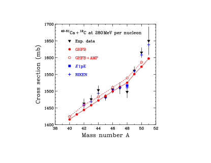
As shown in Fig. 1, the predicted results reproduce the data Tanaka:2019pdo in a level. This indicates that the Kyushu -matrix folding model with the GHFB and GHFB+AMP densities is good.
Our purpose is to redetermine the from the with the Kyushu (chiral) -matrix folding model. The Kyushu -matrix folding model (the GHFB and GHFB+AMP densities) is much better than the optical limit of the Glauber model (the Woos-Saxon densities).
We scale the GHFB and GHFB+AMP densities so that the of the scaled densities can agree with the central values of under the condition that the proton radius of the scaled proton density equals the data Angeli:2013epw determined from the isotope shift based on the electron scattering.
II Model
II.1 Folding model
In the -matrix folding model, the potential consists of the direct and the exchange part defined in Ref. Sumi:2012fr :
| (1) | |||||
| (2) | |||||
where for the coordinate between a projectile (P) and a target (T). The coordinate () denotes the location for the interacting nucleon measured from the center-of-mass of P (T). Each of and stands for the -component of isospin; 1/2 means neutron and 1/2 does proton. The original form of is a non-local function of , but it has been localized in Eq. (2) with the local semi-classical approximation Brieva-Rook in which P is assumed to propagate as a plane wave with the local momentum within a short range of the nucleon-nucleon interaction, where for the mass number () of P (T). The validity of this localization is shown in Ref. Minomo:2009ds .
The direct and exchange parts, and , of the matrix are described by
| (3) | |||
| (4) |
where the are the spin-isospin (-) components of the -matrix interaction and . As a way of the center-of-mass (cm) corrections in the proton and neutron densities, we take the method of Ref. Sumi:2012fr , since it is very simple. As for 12C, we use a phenomenological density of Ref. C12-density . As for Ca isotopes, we take the densities scaled from the GHFB and GHFB+AMP densities.
II.2 GHFB and GHFB+AMP
In GHFB+AMP, the total wave function with the AMP is defined by
| (5) |
where is the angular-momentum-projector and the for are mean-field (GHFB) states, where is the number of the states. The coefficients are determined by solving the following Hill-Wheeler equation,
| (6) |
with the Hamiltonian and norm kernels defined by
| (7) |
For odd nuclei, we have to put a quasi-particle in a level, but the number of the blocking states are quite large. It is difficult to solve the Hill-Wheeler equation with large . Furthermore, we have to confirm that the resulting converges with respect to increasing for any set of two deformations and . This procedure is quite time-consuming. For this reason, it is not feasible to perform the AMP for odd nuclei. As for GHFB, we consider the one-quasiparticle state that yields the lowest energy, so that we do not have to solve the Hill-Wheeler equation. However, it is not easy to find the values of and at which the energy becomes minimum in the - plane.
For even nuclei, there is no blocking state in the Hill-Wheeler equation. We can thus consider GHFB+AMP. However, we have to find the value of at which the ground-state energy becomes minimum. In this step, the AMP has to be performed for any , so that the Hill-Wheeler calculation is still heavy. In fact, the AMP is not taken for most of mean field calculations; see for example Ref. HP:AMEDEE . The reason why we do not take into account deformation is that the deformation does not affect Sumi:2012fr .
II.3 The scaling of the GHFB and GHFB+AMP densities
We explain the scaling of original density . We can obtain the scaled density from the original one as
| (8) |
with a scaling factor
| (9) |
For later convenience, we refer to the proton (neutron) radius of the scaled density as ( ).
III Results
III.1 42-51Ca
Table 2 show theoretical radii determined with GHFB and GFHB+AMP for 39-64Ca. Effects of the AMP are small for radii.
| 39 | 3.320 | 3.381 | 3.351 | -0.061 | ||||
|---|---|---|---|---|---|---|---|---|
| 40 | 3.366 | 3.412 | 3.389 | -0.046 | 3.349 | 3.393 | 3.371 | -0.044 |
| 41 | 3.387 | 3.397 | 3.392 | -0.010 | ||||
| 42 | 3.451 | 3.424 | 3.438 | 0.026 | 3.417 | 3.401 | 3.409 | -0.010 |
| 43 | 3.448 | 3.405 | 3.428 | 0.043 | ||||
| 44 | 3.501 | 3.426 | 3.467 | 0.075 | 3.477 | 3.410 | 3.447 | 0.067 |
| 45 | 3.504 | 3.414 | 3.465 | 0.090 | ||||
| 46 | 3.555 | 3.436 | 3.504 | 0.118 | 3.530 | 3.420 | 3.483 | 0.110 |
| 47 | 3.554 | 3.424 | 3.499 | 0.130 | ||||
| 48 | 3.604 | 3.445 | 3.539 | 0.159 | 3.576 | 3.428 | 3.515 | 0.148 |
| 49 | 3.621 | 3.440 | 3.548 | 0.181 | ||||
| 50 | 3.687 | 3.469 | 3.601 | 0.218 | 3.658 | 3.452 | 3.577 | 0.206 |
| 51 | 3.698 | 3.462 | 3.607 | 0.236 | ||||
| 52 | 3.760 | 3.490 | 3.659 | 0.270 | 3.734 | 3.475 | 3.659 | 0.270 |
| 53 | 3.779 | 3.486 | 3.671 | 0.293 | ||||
| 54 | 3.840 | 3.524 | 3.726 | 0.316 | 3.817 | 3.507 | 3.705 | 0.310 |
| 55 | 3.856 | 3.524 | 3.739 | 0.332 | ||||
| 56 | 3.913 | 3.557 | 3.790 | 0.357 | 3.891 | 3.541 | 3.770 | 0.350 |
| 57 | 3.928 | 3.557 | 3.802 | 0.370 | ||||
| 58 | 3.977 | 3.588 | 3.847 | 0.389 | 3.958 | 3.575 | 3.830 | 0.383 |
| 59 | 3.995 | 3.593 | 3.863 | 0.402 | ||||
| 60 | 4.043 | 3.611 | 3.904 | 0.432 | 4.020 | 3.608 | 3.888 | 0.412 |
| 62 | 4.106 | 3.637 | 3.961 | 0.469 | 4.067 | 3.628 | 3.931 | 0.439 |
| 64 | 4.153 | 3.658 | 4.005 | 0.494 | 4.113 | 3.648 | 3.974 | 0.465 |
As proton and neutron densities, we use GHFB for odd nuclei and GHFB+AMP for even nuclei, and scale the GHFB and GHFB+AMP densities so that the scaled proton and neutron radii may agree with Angeli:2013epw of electron scattering and , respectively; namely and .
Figure 1 shows mass-number () dependence of for 42-51Ca scattering on a 12C target at 280 MeV per nucleon. The folding model with GHFB and GHFB+AMP densities (open and closed circles) reproduce the data Tanaka:2019pdo in a 2 level, indicating that the folding model is reliable. This allows us to scale the proton and neutron densities calculated with GHFB and GHFB+AMP so as to and . The folding-model results () with the scaled densities mentioned above slightly deviate the central values of . The small deviation comes from the method taken.
Now we redetermine , and from the data Tanaka:2019pdo on , using Angeli:2013epw of electron scattering. For this purpose, we scale the proton and neutron densities of GHFB and GHFB+AMP so that the calculated with the scaled densities may agree with the central values of under the condition that . The resulting values and the yield and . Our results are tabulated in Table 3.
| A | fm | fm | fm | fm |
|---|---|---|---|---|
| 42 | ||||
| 43 | 3.397 0.003 | 3.468 0.029 | 3.529 0.05 | 0.132 0.05 |
| 44 | 3.424 0.003 | 3.511 0.030 | 3.582 0.05 | 0.158 0.05 |
| 45 | 3.401 0.003 | 3.452 0.026 | 3.493 0.05 | 0.092 0.05 |
| 46 | 3.401 0.003 | 3.489 0.026 | 3.555 0.05 | 0.154 0.05 |
| 47 | 3.384 0.003 | 3.488 0.034 | 3.563 0.06 | 0.179 0.06 |
| 48 | 3.385 0.003 | 3.447 0.035 | 3.490 0.06 | 0.105 0.06 |
| 49 | 3.400 0.003 | 3.568 0.028 | 3.679 0.05 | 0.279 0.05 |
| 50 | 3.429 0.003 | 3.658 0.031 | 3.803 0.05 | 0.374 0.05 |
| 51 | 3.445 0.003 | 3.713 0.066 | 3.877 0.10 | 0.432 0.10 |
III.2 48Ca
We consider , since is related to the slope parameter in neutron matter Tagami:2020shn . As a measurement on skin , the high-resolution polarizability experiment (pE) was made for 48Ca Birkhan:2016qkr in RCNP. The result is
| (10) |
For , the measurement is most reliable in the present stage. The central value 0.17 fm of Eq. (10) yields matter radius fm and neutron radius fm from proton radius fm evaluated with the isotope shift method based on the electron scattering Angeli:2013epw . We then scale the proton and neutron densities calculated with GHFB+AMP so as to reproduce and . In Fig. 1, the calculated with the scaled densities is near the upper bound of .
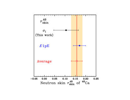
We take the weighted mean and its error for fm and our result fm. The final result is
| (11) |
Our final result is shown in Fig. 2, together with fm and our result fm.
As an ab initio method for Ca isotopes, we should consider the coupled-cluster method Hagen:2013nca ; Hagen:2015yea with chiral interaction. Chiral interactions were constructed by two groups Weinberg:1991um ; Epelbaum:2008ga ; Machleidt:2011zz . The coupled-cluster result Hagen:2015yea
| (12) |
is consistent with our final result of Eq. (11).
IV Discussions
Mass-number dependence of has a kink at . The data on hardly depend on , as shown in Table 4; note that is the binding energy of a nucleus. Here, the central values of data on and are taken from Refs. Tanaka:2019pdo ; HP:NuDat 2.8 . In fact, the deviation of is much smaller than the average value; namely,
| (13) |
for 42-51Ca. This indicates that is in inverse proportion to as an experimental result.
| A | fm | MeV | |
|---|---|---|---|
| 42 | 3.437 | 8.616563 | 0.1501 |
| 43 | 3.453 | 8.600663 | 0.1505 |
| 44 | 3.492 | 8.658175 | 0.1532 |
| 45 | 3.452 | 8.630545 | 0.1510 |
| 46 | 3.487 | 8.66898 | 0.1532 |
| 47 | 3.491 | 8.63935 | 0.1528 |
| 48 | 3.471 | 8.666686 | 0.1524 |
| 49 | 3.565 | 8.594844 | 0.1553 |
| 50 | 3.645 | 8.55016 | 0.1579 |
| 51 | 3.692 | 8.476913 | 0.1586 |
For , the difference between and the central value of may come from that between reaction cross section and interaction cross section, i.e., mb. We assume that the difference mb for 48Ca is the same as for 42-51Ca. The estimated is +18.5 mb in which the error on the estimated is % larger than the error % on ; as a good experiment on , we can consider 9Be, 12C, 27Al+12C scattering of Ref. Takechi:2009zz and the error is %. The figure 3 is shown below.
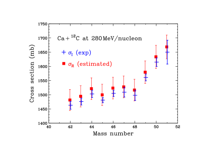
Now we assume that +18.5 mb as the data for 42-51Ca. Using the estimated instead of , we take the same procedure in order to obtain . As shown in Table 5, the resulting is almost the same as the of Ref. Tanaka:2019pdo , except for 48Ca. As for 48Ca, our estimates value 0.170 0.06 fm agrees with of Ref. Birkhan:2016qkr .
| A | ||
|---|---|---|
| 42 | ||
| 43 | 0.104 0.05 | 0.103 0.05 |
| 44 | 0.124 0.05 | 0.125 0.05 |
| 45 | 0.091 0.05 | 0.092 0.05 |
| 46 | 0.151 0.05 | 0.151 0.05 |
| 47 | 0.184 0.06 | 0.184 0.06 |
| 48 | 0.170 0.06 | 0.146 0.06 |
| 49 | 0.275 0.05 | 0.275 0.05 |
| 50 | 0.353 0.05 | 0.353 0.05 |
| 51 | 0.398 0.10 | 0.399 0.10 |
V Summary
Recently, Tanaka el al. measured in RIKEN for 42-51Ca+ 12C scattering at 280 MeV per nucleon, and determined neutron skins for 42-51Ca from the , using the optical limit of the Glauber model with the Woos-Saxon densities Tanaka:2019pdo . We redetermine , , for 42-51Ca, using the Kyushu folding model with the proton and neutron densities scaled from the GHFB and GHFB+AMP densities.
The calculated with the GHFB and GHFB+AMP densities almost reproduce the data Tanaka:2019pdo on . This allows us to determine from the central values of by scaling the proton and neutron densities. The thus determined are close to the original ones of Ref. Tanaka:2019pdo , except for ; see Table 1 for the original values and Table 3 for ours. The thus determined are close to the original results , except for 48Ca. Our experimental values on , , for 42-51Ca are summarized in Table 3.
For 48Ca, our value is fm, while Birkhan et. al. determined fm Birkhan:2016qkr from the high-resolution polarizability experiment (E1pE). We then take the weighted mean and its error for the two values. The resulting value fm is our final value for 48Ca. The value is related to CREX that is ongoing.
Acknowledgements
We thank Dr. Tanaka and Prof. Fukuda for providing the data and helpful comments. M. Y. thanks Dr. M. Toyokawa heartily.
References
- (1) M. Tanaka et al., Phys. Rev. Lett. 124, 102501 (2020). [arXiv:1911.05262 [nucl-ex]].
- (2) F. A. Brieva and J. R. Rook, Nucl. Phys. A 291, 299 (1977); ibid. 291, 317 (1977); ibid. 297, 206 (1978).
- (3) K. Amos, P. J. Dortmans, H. V. von Geramb, S. Karataglidis, and J. Raynal, in Advances in Nuclear Physics, edited by J. W. Negele and E. Vogt(Plenum, New York, 2000) Vol. 25, p. 275.
- (4) T. Furumoto, Y. Sakuragi, and Y. Yamamoto, Phys. Rev. C 78, 044610 (2008).
- (5) K. Minomo, T. Sumi, M. Kimura, K. Ogata, Y. R. Shimizu and M. Yahiro, Phys. Rev. Lett. 108, 052503 (2012), [arXiv:1110.3867 [nucl-th]].
- (6) M. Toyokawa, K. Minomo and M. Yahiro, Phys. Rev. C 88, no. 5, 054602 (2013), [arXiv:1304.7884 [nucl-th]].
- (7) M. Toyokawa, K. Minomo, M. Kohno and M. Yahiro, J. Phys. G 42, no. 2, 025104 (2015), Erratum: [J. Phys. G 44, no. 7, 079502 (2017)] [arXiv:1404.6895 [nucl-th]].
- (8) M. Toyokawa, M. Yahiro, T. Matsumoto, K. Minomo, K. Ogata and M. Kohno, Phys. Rev. C 92, no. 2, 024618 (2015), Erratum: [Phys. Rev. C 96, no. 5, 059905 (2017)], [arXiv:1507.02807 [nucl-th]].
- (9) M. Toyokawa, M. Yahiro, T. Matsumoto and M. Kohno, PTEP 2018, 023D03 (2018), [arXiv:1712.07033 [nucl-th]]. See http://www.nt.phys.kyushu-u.ac.jp/english/gmatrix.html for Kyushu -matrix.
- (10) T. Sumi, K. Minomo, S. Tagami, M. Kimura, T. Matsumoto, K. Ogata, Y. R. Shimizu and M. Yahiro, Phys. Rev. C 85, 064613 (2012), [arXiv:1201.2497 [nucl-th]].
- (11) K. Egashira, K. Minomo, M. Toyokawa, T. Matsumoto and M. Yahiro, Phys. Rev. C 89, 064611 (2014). [arXiv:1404.2735 [nucl-th]].
- (12) S. Watanabe et al., Phys. Rev. C 89, no. 4, 044610 (2014), [arXiv:1404.2373 [nucl-th]].
-
(13)
M. Kohno,
Phys. Rev. C 88, 064005 (2013).
M. Kohno, Phys. Rev. C 96, 059903(E) (2017). - (14) H. V. von Geramb, K. Amos, L. Berge, S. Bräutigam, H. Kohlhoff and A. Ingemarsson, Phys. Rev. C 44, 73 (1991).
- (15) P. J. Dortmans and K. Amos, Phys. Rev. C 49, 1309 (1994).
- (16) S. Tagami, M. Tanaka, M. Takechi, M. Fukuda and M. Yahiro, Phys. Rev. C 101, no. 1, 014620 (2020), [arXiv:1911.05417 [nucl-th]].
- (17) C. Simenel, Lect. Notes Phys. 875, 95-145 (2014) doi:10.1007/978-3-319-01077-9_4 [arXiv:1211.2387 [nucl-th]].
- (18) I. Angeli and K. P. Marinova, Atom. Data Nucl. Data Tabel. 99, 69 (2013).
- (19) K. Minomo, K. Ogata, M. Kohno, Y. R. Shimizu, and M. Yahiro, J. Phys. G 37, 085011 (2010) [arXiv:0911.1184 [nucl-th]].
- (20) H. de Vries, C. W. de Jager, and C. de Vries, At. Data Nucl. Data Tables 36, 495 (1987).
- (21) S. Hilaire and M. Girod, Hartree-Fock-Bogoliubov results based on the Gogny force; http://www-phynu.cea.fr/science-en-ligne/carte-potentiels-microscopiques/carte-potentiel-nucleaire-eng.htm.
- (22) S. Tagami, N. Yasutake, M. Fukuda and M. Yahiro, [arXiv:2003.06168 [nucl-th]].
- (23) J. Birkhan et al., Phys. Rev. Lett. 118, no. 25, 252501 (2017), [arXiv:1611.07072 [nucl-ex]].
- (24) G. Hagen et al., Nature Phys. 12, 186 (2015), [arXiv:1509.07169 [nucl-th]].
- (25) G. Hagen, T. Papenbrock, M. Hjorth-Jensen and D. J. Dean, Rept. Prog. Phys. 77, 096302 (2014), [arXiv:1312.7872 [nucl-th]].
- (26) S. Weinberg, Nucl. Phys. B 363, 3 (1991).
- (27) E. Epelbaum, H. W. Hammer and U. G. Meissner, Rev. Mod. Phys. 81, 1773 (2009). [arXiv:0811.1338 [nucl-th]].
- (28) R. Machleidt and D. R. Entem, Phys. Rept. 503, 1 (2011), [arXiv:1105.2919 [nucl-th]].
- (29) the National Nuclear Data Center, NuDat 2.8; https://www.nndc.bnl.gov/nudat2/.
- (30) M. Takechi, M. Fukuda, M. Mihara, K. Tanaka, T. Chinda, T. Matsumasa, M. Nishimoto, R. Matsumiya, Y. Nakashima and H. Matsubara, et al. Phys. Rev. C 79 (2009), 061601 doi:10.1103/PhysRevC.79.061601