An Approximation Scheme for Multivariate Information
based on Partial Information Decomposition

Abstract

We consider an approximation scheme for multivariate information assuming that synergistic information only appearing in higher order joint distributions is suppressed, which may hold in large classes of systems. Our approximation scheme gives a practical way to evaluate information among random variables and is expected to be applied to feature selection in machine learning. The truncation order of our approximation scheme is given by the order of synergy. In the classification of information, we use the partial information decomposition of the original one. The resulting multivariate information is expected to be reasonable if higher order synergy is suppressed in the system. In addition, it is calculable in relatively easy way if the truncation order is not so large. We also perform numerical experiments to check the validity of our approximation scheme.

I Introduction

Mutual information doi:10.1002/j.1538-7305.1948.tb01338.x is one of the fundamental measures which captures information between two sectors. Even when each sector contains a lot of random variables, the mutual information can give total amount of information between two sectors. One natural question would be how such information is distributed among variables. The framework called the partial information decomposition DBLP:journals/corr/abs-1004-2515 provides a way to decompose mutual information into combinations of partial information in the form of unique, redundant and synergistic information.

In practical point of view, the mutual information may have some difficulties in multivariate and small sample cases. For example, when the number of samples is much smaller than that of possible realizations, it is hard to estimate the mutual information precisely. This is because the mutual information depends on joint probability with a lot of arguments and such a probability is hard to estimate in small sample cases. Thus, it might be good to have an approximation scheme for mutual information that overcome some difficulties.

When we construct an approximation scheme, we need to identify a kind of small quantities in the system. In the multivariate information, one natural assumption would be that information only appearing in higher order synergies is suppressed. Though this assumption would be expected to hold in large classes of systems, we have to specify what is information in higher order synergy. The framework of partial information decomposition gives one solution of this specification.

In this paper, we consider an approximation scheme for mutual information with a lot of variables. We rely on the assumption of suppression of information in higher order parts and construct an approximation scheme based on the partial information decomposition. The resulting approximation scheme is expected to be reasonable if information in higher order synergies is suppressed. In addition, it is calculable in practice when truncation order is not so large.

This paper is organized as follows. In sec. II, we show an overview of the partial information decomposition. In sec. III, we derive our approximation scheme for mutual information. In sec. IV, we perform some numerical experiments to see the validity of our scheme. Sec. V is devoted to discussions.

II Overview of Partial Information Decomposition

Let $X_{1},..,X_{N},Y$ be random variables. For simplicity, we assume all random variables take discrete values and have finite state spaces. Throughout this paper, we regard $X_{1},..,X_{N}$ as feature variables and $Y$ as a target variable. For a given set of feature variables $\{X_{i_{1}},..,X_{i_{m}}\}$, the mutual information on the target variable $Y$ is defined to be

$$MI (X_{i_{1}},..,X_{i_{m}}:Y)$$

$$=\sum_{x_{i_{1}},..,x_{i_{m}},y}p(x_{i_{1}},..,x_{i_{m}},y)\log\frac{p(x_{i_{1}},..,x_{i_{m}},y)}{p(x_{i_{1}},..,x_{i_{m}})p(y)},$$ (1)

where $p$ denotes probability and small letters indicate values of corresponding random variables. The mutual information measures the amount of information about the target variable $Y$ contained in selected features. Though the mutual information can give us the total amount of information in features, it might not be clear how the information is distributed among features $X_{i_{1}},..,X_{i_{m}}$.

The framework of partial information decomposition (PID) can decompose the total amount of information and gives how the information is distributed. Here, we briefly show an overview of this framework and refer to DBLP:journals/corr/abs-1004-2515 for more details. In PID framework, the total amount of information is decomposed into unique, redundant and synergistic information that are associated with combinations of feature variables. Fig. 1 shows decomposition for two feature variable case $X_{1},X_{2}$ and this kind of diagram is denoted as partial information diagram. The region $\{12\}$ is corresponding to synergistic information between $X_{1}$ and $X_{2}$. The region $\{1\}$ or $\{2\}$ is corresponding to unique information of $X_{1}$ or $X_{2}$ respectively. The region $\{1\}\{2\}$ is redundant information between $X_{1}$ and $X_{2}$. Similarly, fig. 2 indicates the information decomposition of three feature variable case $X_{1},X_{2},X_{3}$. In this figure, the mutual information is also decomposed into combinations of feature variables. For example, the region $\{3\}\{12\}$ is corresponding to the unique part of the redundant information between $X_{3}$ and joint variable $(X_{1},X_{2})$.

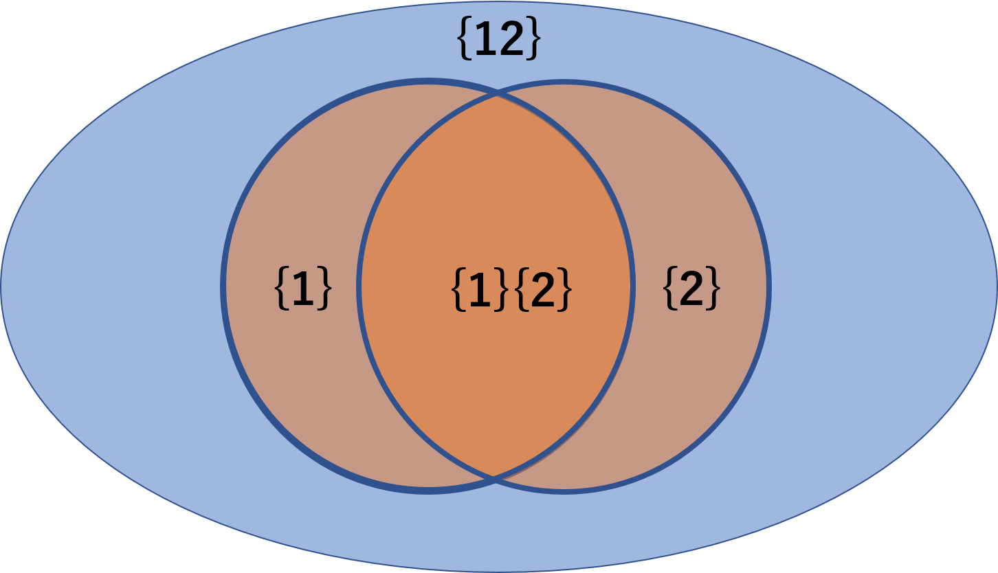
Figure 1: A partial information diagram for two feature variable case.

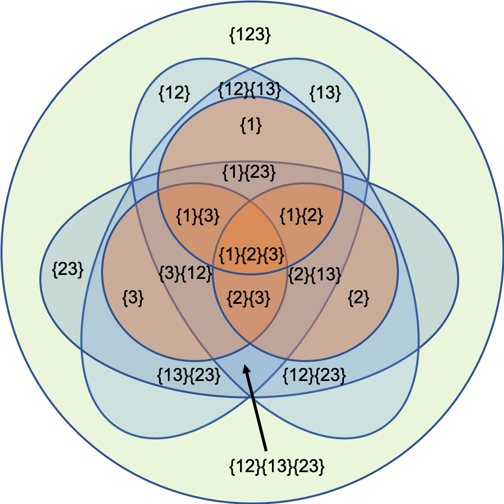
Figure 2: A partial information diagram for three feature variable case.

The key function to determine this kind of information decomposition is the redundancy information $I_{\cap}(Y:A_{1},..,A_{k})$ that measures information about $Y$ contained in all $A_{1},..,A_{k}$, where each $A_{i}$ is a subset of $\{X_{1},..,X_{N}\}$. Once $I_{\cap}$ is defined, every piece of partial information is determined. In the original paper DBLP:journals/corr/abs-1004-2515 , the redundancy information is denoted as $I_{\rm min}$ and defined to be

$$I_{\rm min}(Y:A_{1},..,A_{k})=\sum_{y}p(y)\min_{A_{i}}I(Y=y:A_{i}),$$ (2)

where $I(Y=y,A_{i})$ measures the information associated with a given outcome $y$ of $Y$:

$$I(Y=y:A_{i})=\sum_{a_{i}}p(a_{i}|y)\left[\log\frac{1}{p(y)}-\log\frac{1}{p(y|a_{i})}\right].$$ (3)

This redundancy information $I_{\min}$ satisfies some basic axioms and has good features. For example, each part of partial information is ensured to be non-negative. However, it is known that $I_{\min}$ sometimes gives unintuitive results and several alternatives have been discussed and proposed in the literature in order to overcome drawbacks DBLP:journals/corr/abs-1303-3440 ; DBLP:journals/corr/abs-1210-5902 ; DBLP:journals/corr/abs-1207-2080 ; DBLP:journals/corr/abs-1205-4265 ; DBLP:journals/corr/BertschingerROJA13 ; DBLP:journals/corr/RauhBOJ14 ; jisaku1 ; DBLP:journals/corr/PerroneA15 ; DBLP:journals/corr/RosasNEPV15 ; DBLP:journals/corr/GriffithCJEC13 ; DBLP:journals/corr/GriffithH14 ; DBLP:journals/corr/QuaxHS16 ; DBLP:journals/corr/Barrett14 ; Chicharro2017QuantifyingMR ; Finn2018PointwisePI ; Kolchinsky2019ANA ; Ay2019InformationDB ; Sigtermans2020API . Nevertheless, in practical point of view, $I_{\rm min}$ would be still attractive because the structure is relatively simple and it requires relatively small computational costs. In this paper, we use $I_{\rm min}$ to define an approximation scheme for multivariate information.

For later convenience, we consider union information $I_{\cup}(Y:A_{1},..,A_{k})$, that measures information contained in any of $A_{i}$. For simplicity, we use a shorthand notation $I_{\cup}(Y,\{A_{i}\})\equiv I_{\cup}(Y:A_{1},..,A_{k})$. The principle of inclusion and exclusion gives

$$I_{\cup}(Y:\{A_{i}\}) =\sum_{i}I_{\rm min}(Y:A_{i})-\sum_{i<j}I_{\rm min}(Y:A_{i},A_{j})$$

$$+\sum_{i<j<k}I_{\rm min}(Y:A_{i},A_{j},A_{k})\cdots.$$ (4)

For further computations, the maximum-minimum identity is useful. The identity states that for a given set of numbers $B=\{b_{1},b_{2},..\}$, we have

$${\rm max}~{}B =\sum_{i}{\rm min}(b_{i})-\sum_{i<j}{\rm min}(b_{i},b_{j})$$

$$+\sum_{i<j<k}{\rm min}(b_{i},b_{j},b_{k})+\cdots.$$ (5)

With this identity, we obtain a simple expression of $I_{\cup}$:

$$I_{\cup}(Y:\{A_{i}\}) =\sum_{y}p(y)\max_{A_{i}}I(Y=y:A_{i}).$$ (6)

III An Approximation scheme in terms of synergistic order

In practical point of view, a mutual information with a lot of feature variables would have some disadvantages. For example, it would require a lot of computational costs. In addition, if sample size is not so large, it would be hard to estimate mutual information precisely. Thus, it might be good to have a reasonable approximation which overcomes some of these disadvantages.

In order to construct an approximation scheme, we have to specify a kind of small quantities in the system based on some reasonable assumption. In our case, one natural assumption might be that information only appearing in higher order synergistic part is assumed to be small. This assumption leads us to an approximation scheme whose accuracy is verified by smallness of higher order synergies. Here, we denote the order of synergy as a number of joint features involved. For example, the order of synergy for the element $\{23\}$ in fig. 2 is two.

Next, let us relate the order of synergy to an approximation scheme. We denote a set of set of feature variables that contains just $n$ types of features as $C^{(n)}$. For example, we have $C^{(1)}=\{\{X_{1}\},\{X_{2}\},...\}$ and $C^{(2)}=\{\{X_{1},X_{2}\},\{X_{1},X_{3}\},..\}$. We define $I^{(k)}\equiv I_{\cup}(Y:C^{(k)})$ as the total amount of information that takes synergistic information up to $k$ joint features into account. For example, $I_{\cup}(Y:C^{(1)})$ could be interpreted as the total amount of information without any synergy between feature variables. $I_{\cup}(Y:C^{(2)})$ could be regarded as the total amount of information that takes any pairs of synergistic information into account. $I^{(N)}$ is corresponding to the multivariate information of whole feature variables $X_{1},..,X_{N}$. The difference

$$\Delta^{(k+1)}=I^{(N)}-I^{(k)},$$ (7)

would be interpreted as the total amount of information that only appears in the synergistic information involved by more than $k$ features. Fig. 3 and fig. 4 are corresponding to information contained in $I^{(1)}$ and $I^{(2)}$ respectively for three variable case. By using Eq. (6), the quantity $I^{(k)}$ can be written as

$$I^{(k)}=\sum_{y}p(y)\max_{C_{i}^{(k)}\in C^{(k)}}I(Y=y:C_{i}^{(k)}),$$ (8)

where $C_{i}^{(k)}$ denotes an element in the set $C^{(k)}$.

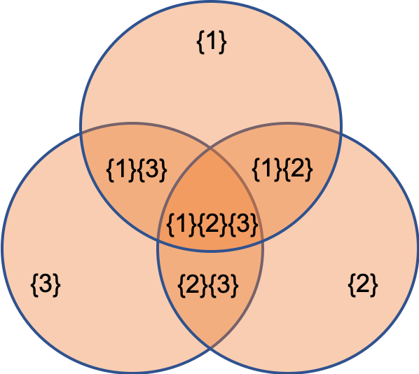
Figure 3: Information contained in $I^{(1)}$ for three feature variable case.

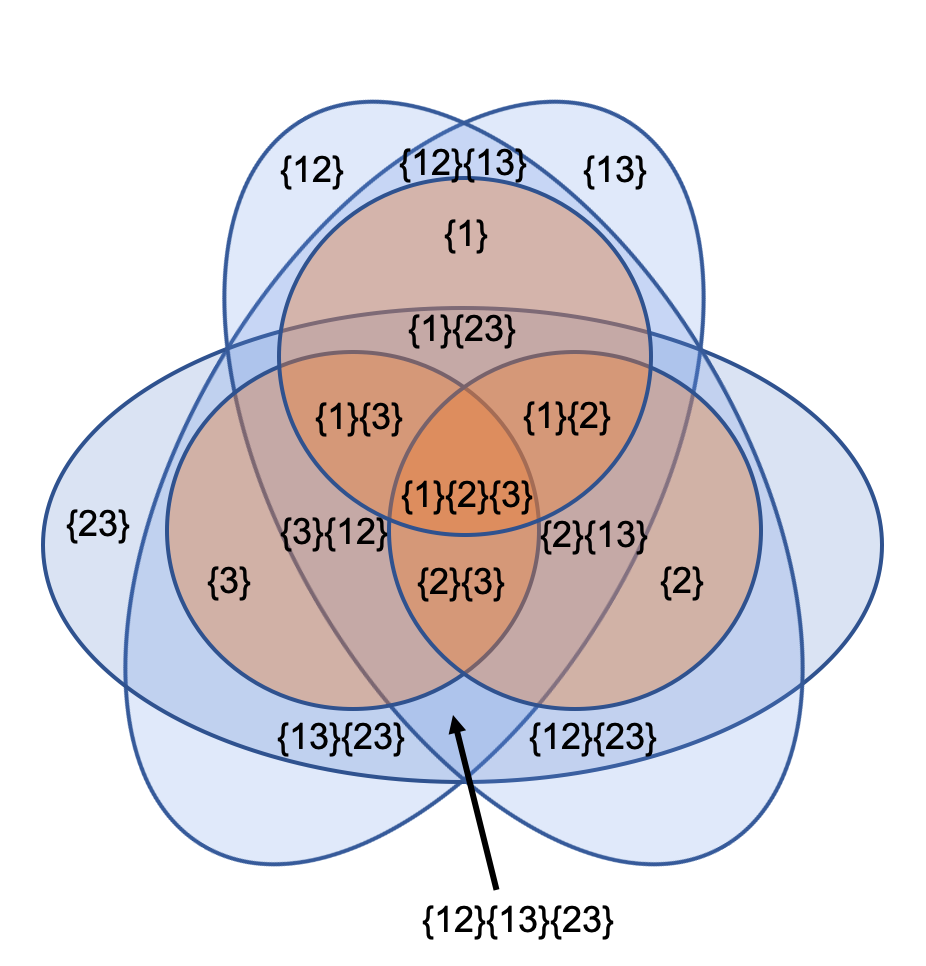
Figure 4: Information contained in $I^{(2)}$ for three feature variable case.

The quantity $I^{(k)}$ has following features:

• Each $I^{(k)}$ has a corresponding region in the partial information diagram.

• $I^{(k)}$ is increasing function in terms of $k$

• $I^{(k)}$ only depends on joint probability functions whose number of arguments are $k+1$: ($p(y,x_{i_{1}},..,x_{i_{k}})$).

• Lower order $I^{(k)}$ is expected to be stable against small sample size because it does not depend on joint probabilities with large number of arguments.

• If higher order synergistic information is small, low order $I^{(k)}$ is expected to give a reasonable approximation of the total mutual information.

Considering these features, collection of $I^{(k)}$ might be regarded as an approximation scheme for the total mutual information.

Finally, let us comment on the feature selection using $I^{(k)}$. The feature selection based on mutual information seems promising and a lot of methods has been derived in the literature (see for example DBLP:journals/corr/VergaraE15 ; jisaku3 ; DBLP:journals/corr/abs-1907-07384 ). The feature selection based on $I^{(k)}$ would become a new one. One simple way to determine important features based on $I^{(k)}$ may be as follows. For a given order $k$ that is not so large, we can estimate $I^{(k)}$ for all features. Then, Some of features may not contribute to $I^{(k)}$. This is because number of features that is chosen in max operation in Eq. (8) is limited. We delete such irrelevant features and obtain a set of features that is relevant in $I^{(k)}$. If number of features is still large, we may delete additional features by referring to $I^{(k)}$ with lower number of features.

IV Numerical Results

In this section, we perform two numerical experiments in a simple setup. The first experiment is intended to see behavior of exact $I^{(k)}$. The second one is to see effects of finite sample size.

Let $s_{1},s_{2}..,s_{M}$ be bit type random variables whose values are $0$ or $1$. We set the joint probability $p(s_{1},..,s_{M})$ as follows.

$$p(s_{1},..,s_{M}) =\frac{e^{A(s_{1},..,s_{M})}}{Z},$$ (9)

$$Z =\sum_{s_{1},..,s_{M}}e^{A(s_{1},..,s_{M})},$$ (10)

$$A(s_{1},..,s_{M}) =\epsilon_{0}\sum_{i}a_{i}\cdot s_{i}+\epsilon_{1}\sum_{i<j}b_{ij}\cdot(s_{i}\oplus s_{j})$$

$$+\epsilon_{2}\sum_{i<j<k}c_{ijk}\cdot(s_{i}\oplus s_{j}\oplus s_{k}),$$ (11)

where $\oplus$ denotes XOR operation, $\epsilon_{0},\epsilon_{1},\epsilon_{2},a_{i},b_{ij},c_{ijk}$ are real number coefficients. In the experiments, we set $M=8$ and each number $a_{i}$, $b_{ij}$ or $c_{ijk}$ is picked up from an uniform random variable whose range is from $-1$ to $1$. We regard last three components as the target variable $Y=(s_{6},s_{7},s_{8})$ and the others as the feature variables $X_{i}=s_{i},(i=1,..,5)$.

In the first experiment, we calculate exact $I^{(k)}$. We set $\epsilon_{0}=1,\epsilon_{1}=1/2,\epsilon_{2}=1/10$ in order to suppress higher order interactions. By resampling coefficients $a_{i},b_{ij},c_{ijk}$ from an uniform random variable from $-1$ to $1$, we calculate $I^{(k)}$ for each setup. Fig. 5 shows results of $I^{(k)}$ normalized by $I^{(5)}$. Note that $I^{(5)}$ is equal to the total mutual information and typically take values around $0.1-0.2$. We take 10 different coefficient sets and plot them. We can see that $I^{(k)}$ is actually increasing function. In addition, upward convex curves of each result indicate the suppression of information in higher order synergistic part.

We also check the behavior of $I^{(k)}$ under the situation where higher order interactions dominate over lower order ones. In such a case, our approximation scheme is not expected to work well. We set $\epsilon_{0}=1/10$, $\epsilon_{1}=1/100$ and $\epsilon_{2}=2$. We take $a_{i},b_{ij},c_{ijk}$ from an uniform random variable from $-1$ to $1$. Then, we set $b_{ij}$ and $c_{ijk}$ that are not involved by just one target variable to zero. We calculate $I^{(k)}$ for 10 setups. Fig. 6 shows results of $I^{(k)}$ normalized by $I^{(5)}$. Since the dominant interaction terms are ones with $\epsilon_{2}$ involved by one target variable, $I^{(2)}$ becomes much larger than $I^{(1)}$. In this case, the leading order approximation $I^{(1)}$ does not work well.

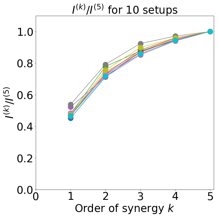
Figure 5: $I^{(k)}$ normalized by the total mutual information $I^{(5)}$ for 10 different setups.

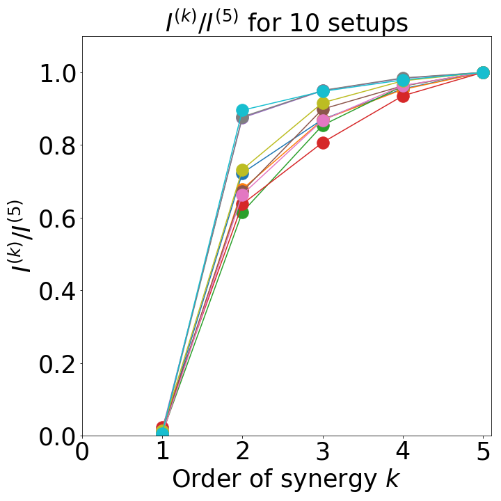
Figure 6: The strong coupling case of $I^{(k)}$ normalized by the total mutual information $I^{(5)}$ for 10 different setups.

The second experiment is intended to see effects of finite sample size. we set $\epsilon_{0}=1,\epsilon_{1}=1/2,\epsilon_{2}=1/10$ again. We first fix the coefficients $a_{i},b_{ij},c_{ijk}$ and calculate exact $I^{(k)}$. Then, we pick up $N_{s}$ samples by using $p(s_{1},..,p_{M})$ and calculate the empirical probability $\hat{p}$. In order to obtain $I^{(k)}$, we have to estimate $I(Y=y:c_{i}^{(k)})$ in Eq. (8). We denote $\hat{I}(Y=y:C_{i}^{(k)})$ as one estimated by the empirical probability. This $\hat{I}(Y=y:C_{i}^{(k)})$ is supposed to have relatively large bias especially for small sample cases . At the leading order in asymptotic expansion, the bias $\delta(y,C_{i}^{(k)})$ would be given by

$$\hat{p}(y)\delta(y,C_{i}^{(k)}) =\sum_{c_{v}}\frac{1}{2N_{s}}[1-\hat{p}(y,c_{v})]$$

$$+\sum_{c_{v}}\frac{\hat{p}(y,c_{v})}{2N_{s}\hat{p}(y)}[1-\hat{p}(y)]$$

$$+\sum_{c_{v}}\frac{\hat{p}(y,c_{v})}{2N_{s}\hat{p}(c_{v})}[1-\hat{p}(c_{v})],$$ (12)

where $c_{v}$ denotes one of the possible values of $C_{i}^{(k)}$. In App. A, we derive this bias correction term. We use bias corrected quantities

$$\hat{I}(Y=y,C_{i}^{(k)})\rightarrow\hat{I}(Y=y,C_{i}^{(k)})-\delta(y,C_{i}^{(k)})$$ (13)

in the estimation of $I^{(k)}$ and the result is denoted by $\hat{I}^{(k)}$. We define a normalized variable as follows.

$$\hat{i}^{(k)}=\frac{\hat{I}^{(k)}}{I^{(k)}}-1.$$ (14)

$\hat{i}^{(k)}$ can be regarded as a random variable against resamplings. For a fixed sample size $N_{s}$, we estimate the mean and standard deviation of $\hat{i}^{(k)}$ that are functions of $N_{s}$. In the estimation of mean and standard deviation, we take 100 time resamplings. Fig. 7 shows mean and standard deviation of $\hat{i}^{(k)}$ as a function of sample size $N_{s}$. The mean value can be regarded as a bias from the true value. In this setup with relatively small sample size, we observe that the bias dominates over standard deviation. We can see that lower order $I^{(k)}$ has less bias and stable when sample size is relatively small.

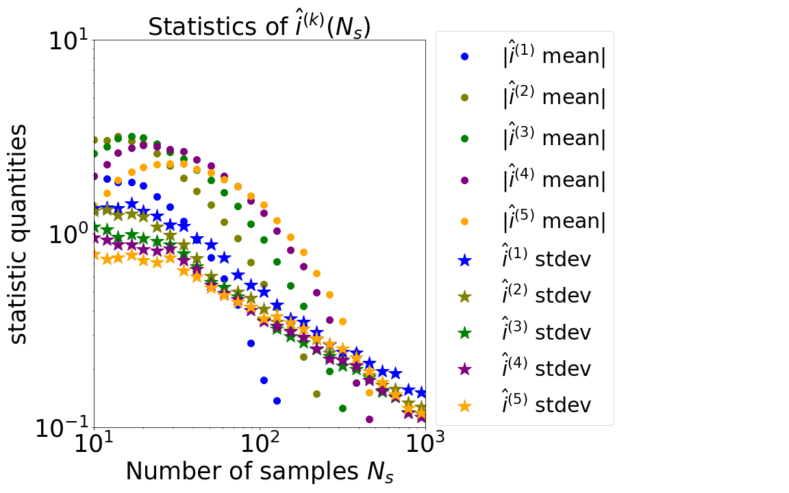
Figure 7: The mean and standard deviation of $\hat{i}^{(k)}$ as a function of sample size $N_{s}$. The term “stdev” is a shorthand notation of standard deviation.

V Discussion

In this paper, we have derived an approximation scheme for multivariate information based on partial information decomposition. The key assumption is that information only appearing in higher order synergy is small and we have constructed truncation scheme for multivariate information in terms of synergistic order. The resulting approximation scheme is expected to be reasonable when the higher order information in the system is suppressed. In addition, it is calculable in practice when the truncation order is not so high. We have also checked properties of our approximation scheme by numerical experiments.

The truncated mutual information $I^{(k)}$ has relatively simple structure. This simplicity is originated from the simple structure of the redundant information $I_{\rm min}(A_{1},..,A_{k})$. Though the quantity $I_{\rm min}$ itself is well defined, $I_{\rm min}$ does not take joint properties between $A_{i}$ into account and it would overestimate the redundant information in some sense. Due to this overestimation, $I^{(k)}$ might underestimate the corresponding information and lead to unintuitive results in some cases. Thus, it might be interesting to define an approximation scheme based on another kind of redundant information $I_{\cap}$.

One direction of application of our approximation scheme would be feature selection in machine learning. Given a truncation order, we can see important features in the system based on $I^{(k)}$. Some of features may not contribute to $I^{(k)}$ and we obtain a minimal set of features that contribute to $I^{(k)}$. As is mentioned above, $I^{(k)}$ potentially underestimate the information, which could cause underestimation of the number of relevant features. In this point of view, the feature selection based on $I^{(k)}$ can be regarded as a conservative one. In any case, it would be interesting to see validity of feature selection based on $I^{(k)}$ in realistic setups and future research will be focused on it.

Appendix A Derivation of bias term

Here, we derive a bias correction term in Eq. (IV). We consider a bias correction for the quantity $\hat{p}(y)\hat{I}(Y=y,C_{i}^{(k)})$. This quantity can be rewritten as follows.

$$\hat{p}(y)\hat{I}(Y=y,C_{i}^{(k)})=\sum_{c_{v}\in C_{i}^{(k)}}\hat{p}(y,c_{v})\log\left(\frac{\hat{p}(y,c_{v})}{\hat{p}(y)\hat{p}(c_{v})}\right),$$ (15)

where $\hat{p}(\cdot)$ denotes empirical probability. For each probability $\hat{p}(\cdot)$, we define deviation term $\Delta(\cdot)$ as follows.

$$\Delta(\cdot)\equiv\frac{\hat{p}(\cdot)-p(\cdot)}{p(\cdot)},$$ (16)

where $p(\cdot)$ denotes the true probability. We expand Eq. (15) up to second order in terms of $\Delta$ and calculate the average of it. In the average calculation, we use properties of the multinomial distribution. Then, the result is given by Eq. (IV).

References

- [1] C. E. Shannon. A mathematical theory of communication. Bell System Technical Journal, 27(3):379–423.
- [2] Paul L. Williams and Randall D. Beer. Nonnegative decomposition of multivariate information. CoRR, abs/1004.2515, 2010.
- [3] Joseph T. Lizier, Benjamin Flecker, and Paul L. Williams. Towards a synergy-based approach to measuring information modification. CoRR, abs/1303.3440, 2013.
- [4] Nils Bertschinger, Johannes Rauh, Eckehard Olbrich, and Jürgen Jost. Shared information – new insights and problems in decomposing information in complex systems. CoRR, abs/1210.5902, 2012.
- [5] Malte Harder, Christoph Salge, and Daniel Polani. A bivariate measure of redundant information. CoRR, abs/1207.2080, 2012.
- [6] Virgil Griffith and Christof Koch. Quantifying synergistic mutual information. CoRR, abs/1205.4265, 2012.
- [7] Nils Bertschinger, Johannes Rauh, Eckehard Olbrich, Jürgen Jost, and Nihat Ay. Quantifying unique information. CoRR, abs/1311.2852, 2013.
- [8] Johannes Rauh, Nils Bertschinger, Eckehard Olbrich, and Jürgen Jost. Reconsidering unique information: Towards a multivariate information decomposition. CoRR, abs/1404.3146, 2014.
- [9] Olbrich Eckehard, Bertschinger Nils, and Rauh Johannes. Information decomposition and synergy. Entropy 17, no. 5. 3501-3517, 2015.
- [10] Paolo Perrone and Nihat Ay. Hierarchical quantification of synergy in channels. CoRR, abs/1512.03614, 2015.
- [11] Fernando Rosas, Vasilis Ntranos, Christopher J. Ellison, Sofie Pollin, and Marian Verhelst. Understanding interdependency through complex information sharing. CoRR, abs/1509.04555, 2015.
- [12] Virgil Griffith, Edwin K. P. Chong, Ryan G. James, Christopher J. Ellison, and James P. Crutchfield. Intersection information based on common randomness. CoRR, abs/1310.1538, 2013.
- [13] Virgil Griffith and Tracey Ho. Quantifying redundant information in predicting a target random variable. CoRR, abs/1411.4732, 2014.
- [14] Rick Quax, Omri Har-Shemesh, and Peter M. A. Sloot. Quantifying synergistic information using intermediate stochastic variables. CoRR, abs/1602.01265, 2016.
- [15] Adam B. Barrett. An exploration of synergistic and redundant information sharing in static and dynamical gaussian systems. CoRR, abs/1411.2832, 2014.
- [16] Daniel Chicharro. Quantifying multivariate redundancy with maximum entropy decompositions of mutual information. arXiv: Data Analysis, Statistics and Probability, 2017.
- [17] Conor Finn and Joseph T. Lizier. Pointwise partial information decomposition using the specificity and ambiguity lattices. Entropy, 20:297, 2018.
- [18] Artemy Kolchinsky. A novel approach to multivariate redundancy and synergy. ArXiv, abs/1908.08642, 2019.
- [19] Nihat Ay, Daniel Polani, and Nathaniel Virgo. Information decomposition based on cooperative game theory. ArXiv, abs/1910.05979, 2019.
- [20] David Sigtermans. A partial information decomposition based on causal tensors. ArXiv, abs/2001.10481, 2020.
- [21] Jorge R. Vergara and Pablo A. Estévez. A review of feature selection methods based on mutual information. CoRR, abs/1509.07577, 2015.
- [22] Mohamed Bennasar, Yulia Hicks, and Rossitza Setchi. Feature selection using joint mutual information maximisation. Expert Syst. Appl., 42, 22 (December 2015), 8520–8532, 2015.
- [23] Mario Beraha, Alberto Maria Metelli, Matteo Papini, Andrea Tirinzoni, and Marcello Restelli. Feature selection via mutual information: New theoretical insights. CoRR, abs/1907.07384, 2019.
- [24] Liam Paninski. Estimation of entropy and mutual information. Neural Comput, 15, 6 (June 2003), 1191-1253, 2003.