Variational Mixture of Normalizing Flows

Abstract

In the past few years, deep generative models, such as generative adversarial networks [6], variational autoencoders [13], and their variants, have seen wide adoption for the task of modelling complex data distributions. In spite of the outstanding sample quality achieved by those early methods, they model the target distributions implicitly, in the sense that the probability density functions induced by them are not explicitly accessible. This fact renders those methods unfit for tasks that require, for example, scoring new instances of data with the learned distributions. Normalizing flows have overcome this limitation by leveraging the change-of-variables formula for probability density functions, and by using transformations designed to have tractable and cheaply computable Jacobians. Although flexible, this framework lacked (until recently semisuplearning_nflows, RAD) a way to introduce discrete structure (such as the one found in mixtures) in the models it allows to construct, in an unsupervised scenario. The present work overcomes this by using normalizing flows as components in a mixture model and devising an end-to-end training procedure for such a model. This procedure is based on variational inference, and uses a variational posterior parameterized by a neural network. As will become clear, this model naturally lends itself to (multimodal) density estimation, semi-supervised learning, and clustering. The proposed model is illustrated on two synthetic datasets, as well as on a real-world dataset.

Keywords: Deep generative models, normalizing flows, variational inference, probabilistic modelling, mixture models.

1 Introduction

1.1 Motivation and Related Work

Generative models based on neural networks – variational autoencoders (VAEs), generative adversarial networks (GANs), normalizing flows, and their variations – have experienced increased interest and progress in their capabilities. VAEs [13] work by leveraging the reparameterization trick to optimize a variational posterior parameterized by a neural network, jointly with the generative model per se - it too a neural network, which takes samples from a latent distribution at its input space and decodes them into the observation space. GANs also work by jointly optimizing two neural networks: a generator, which learns to produce realistic samples in order to “fool” the second network – the discriminator – which learns to distinguish samples produced by the generator from samples taken from real data. GANs [6] learn by having the generator and discriminator “compete”, in a game-theoretic sense. Both VAEs and GANs learn implicit distributions of the data, in the sense that - if training is successful - it is possible to sample from the learned model, but there is no direct access to the likelihood function of the learned distribution.

Normalizing flows [18] differ from VAEs and GANs, among other aspects, in the fact that they allow learning explicit distributions from data. Thus, normalizing flows lend themselves to the task of density estimation.

Less (although some) attention has been given to the extension of these types of models with discrete structure, such as the one found in finite mixtures. Exploiting such structure, while still being able to benefit from the expressiveness of neural generative models – specifically, normalizing flows – is the goal of this work. Specifically, this works explores a framework to learn a mixture of normalizing flows, wherein a neural network classifier is learned jointly with the mixture components. Doing so will naturally produce an approach which performs, not only density estimation, but also clustering, since the classifier can be used to assign points to clusters. Naturally, this approach also allows doing semi-supervised learning, where available labels can be used to refine the classifier and selectively train the mixture components.

The work herein presented intersects several active directions of research. In the sense of combining deep neural networks with probabilistic modelling, particularly with the goal of endowing simple probabilistic graphical models with more expressiveness, [10] and [15] proposed a framework to use neural-network-parameterized likelihoods, composed with latent probabilistic graphical models. Still in line with this topic, but with an approach more focused towards clustering and semi-supervised learning, [2] proposed a VAE-inspired model, where the prior is a Gaussian mixture. Finally, [19] described an unsupervised method for clustering using deep neural networks, which is a task that can also be fulfilled by the model presented in this work.

The two prior publications that are most related to the present work are those by [4] and [9]. As in this paper, [4] tries to reconcile normalizing flows with a multimodal (or discrete) structure. They do so by partitioning the latent space into disjoint subsets, and using a mixture model where each component has non-zero weight exclusively within its respective subset. Then, using a set-identification function and a piece-wise invertible function, a variation of the change-of-variable formula is devised. [9] also exploit a multimodal structure, while using normalizing flows for expressiveness. However, while the present work relies on a variational posterior parameterized by a neural network and learns $K$ flows (one for each mixture component), the method proposed by [9] resorts to a latent mixture of Gaussians as the base distribution for its flow model, and learns a single normalizing flow.

1.2 Contributions

The main contribution of the present work can be summarized as follows: we propose a finite mixture of normalizing flows with a tractable end-to-end learning procedure. We also provide a proof-of-concept implementation to demonstrate the capabilities of such model, and illustrate its working in three different types of leaning tasks: density estimation, clustering, and semi-supervised learning.

We have achieved these goals by proposing a method to learn a mixture of $K$ normalizing flows, through the optimization of a variational inference objective, where the variational posterior is parameterized by a neural network with a softmax output, and its parameters are optimized jointly with those of the mixture components.

1.3 Notation

The main notation used throughout this work is as follows. Scalars and vectors are lower-case letters, with vectors in bold (e.g., $x$ is a scalar, $\mathbf{z}$ is a vector). Upper-case letters represent matrices. Vector $\bm{x}_{a:b}$ contains the $a$-th to the $b$-th elements of vector $\bm{x}$. For distributions, subscript notation will only be used when the distribution is not clear from context. The operator $\odot$ denotes the element-wise product. The letter $x$ is preferred for observations. The letter $z$ is preferred for latent variables. The letter $\bm{\theta}$ is preferred for parameter vectors. A function $g$ of $\bm{x}\in\bm{\mathcal{X}}$, parameterized by $\bm{\theta}$ is written as $g(\bm{x};\bm{\theta})$, when the dependence on $\bm{\theta}$ is to be made explicit.

1.4 Summary

The remaining sections of the paper are organized as follows. Section 2 reviews normalizing flows, which are the central building block of the work herein presented. Section 3 introduces the proposed approach, variational mixtures of normalizing flows (VMoNF), and the corresponding learning algorithm. Finally, experiments are presented in Section 4, and Section 5 concludes the paper with a brief discussion and some pointers for future work.

2 Normalizing Flows

2.1 Introduction

The best-known and most studied probability distributions, which are analitically manageable, are rarely expressive enough for real-world complex datasets, such as images or signals. However, they have properties that make them amenable to work with, for instance, they allow for tractable parameter estimation, they have closed-form likelihood functions, and sampling from them is simple.

One way to obtain more expressive models is to assume the existence of latent variables, leverage certain factorization structures, and use well-known distributions for the individual factors of the product that constitutes the model’s joint distribution. By using these structures and specific, well-chosen combinations of distributions (namely, conjugate prior-likelihood pairs), these models are able to remain tractable - normally via bespoke estimation/inference/learning algorithms.

Another approach to obtaining expressive probabilistic models is to apply transformations to a simple distribution, and use the change of variables formula to compute probabilities in the transformed space. This is the basis of normalizing flows, an approach proposed by [18], and which has since evolved and developed into the basis of multiple state-of-the-art techniques for density modelling and estimation [12], [3], [1], [16].

2.2 Change of Variables

Given a random variable $\bm{z}\in\mathbb{R}^{D}$, with probability density function $f_{Z}$, and a bijective and continuous function $g(\>.\>;\bm{\theta})\ :\ \mathbb{R}^{D}\rightarrow\mathbb{R}^{D}$, the probability density function $f_{X}$ of the random variable $\bm{x}=g(\bm{z})$ is given by

$$f_{X}(\bm{x}) =f_{Z}(g^{-1}(\bm{x};\bm{\theta}))\Big{|}\det\Big{(}\frac{d}{d\bm{x}}g^{-1}(\bm{x};\bm{\theta})\Big{)}\Big{|}$$ (1)

$$=f_{Z}(g^{-1}(\bm{x};\bm{\theta}))\Big{|}\det\Big{(}\frac{d}{d\bm{z}}g(\bm{z};\bm{\theta})\bigg{|}_{\bm{z}=g^{-1}(\bm{x};\bm{\theta})}\Big{)}\Big{|}^{-1},$$ (2)

where $\det\Big{(}\frac{d}{d\bm{x}}g^{-1}(\bm{x};\bm{\theta})\Big{)}$ is the determinant of the Jacobian matrix of $g^{-1}(\>.\>;\bm{\theta})$, computed at $\bm{x}$. Since $g(\>.\>;\bm{\theta})$ is a transformation parameterized by a parameter vector $\bm{\theta}$, this expression can be optimized w.r.t. $\bm{\theta}$, with the goal of making it approximate some arbitrary distribution. For this to be feasible, the following have to be easily computable:

• $f_{Z}$ - the starting probability density function (also called base density). It is assumed that it has a closed-form expression. In practice, this is typically one of the basic distributions (Gaussian, Uniform, etc.)

• $\det\Big{(}\frac{d}{d\bm{x}}g^{-1}(\bm{x};\bm{\theta})\Big{)}$ - the determinant of the Jacobian matrix of $g^{-1}$; for most transformations, this is not “cheap” to compute.

• The gradient of $\det\Big{(}\frac{d}{d\bm{x}}g^{-1}(\bm{x};\bm{\theta})\Big{)}$ w.r.t. $\bm{\theta}$; this is crucial for gradient-based optimization of $\bm{\theta}$ to be feasible. For most cases, this is not easily computable.

As will become clear, the crux of the normalizing flows framework is to find transformations that are expressive enough, and for which the determinants of their Jacobian matrices, as well as the gradients of those determinants are both “cheap” to compute.

2.3 Normalizing Flows

Consider $L$ transformations $h_{\ell}$, for $\ell=0,1,...,L-1$ that fulfill the three requirements listed above. Let each of those transformations be parameterizable by a parameter vector $\bm{\theta}_{\ell}$, for $\ell=0,1,...,L-1$. The dependence on the parameter vectors will be implicit from here on. Let $\bm{z_{\ell}}=h_{\ell-1}\circ h_{\ell-2}\circ...\circ h_{0}(\bm{z_{0}})$, where $\bm{z_{0}}$ is sampled from $f_{Z}$, the base density. Notice that, with this notation, $\bm{z_{L}}=\bm{x}$. Furthermore, let $g$ be the composition of the $L$ transformations. Applying the change of variables formula to

$$\bm{z_{0}} \sim f_{Z}$$ (3)

$$\bm{x} =h_{L-1}\circ h_{L-2}\circ...\circ h_{0}(\bm{z_{0}}),$$ (4)

noting that $g^{-1}=h^{-1}_{0}\circ h^{-1}_{1}\circ...\circ h^{-1}_{L-1}$ and using the chain rule for derivatives, leads to

$$f_{X}(\bm{x}) =f_{Z}(g^{-1}(\bm{x}))\Big{|}\det\Big{(}\frac{d}{d\bm{x}}g^{-1}(\bm{x})\Big{)}\Big{|}$$ (5)

$$=f_{Z}(g^{-1}(\bm{x}))\prod_{\ell=0}^{L-1}\Big{|}\det\Big{(}\frac{d}{d\bm{z_{\ell+1}}}h_{\ell}^{-1}(\bm{z_{\ell+1}})\Big{)}\Big{|}$$ (6)

$$=f_{Z}(g^{-1}(\bm{x}))\prod_{\ell=0}^{L-1}\Big{|}\det\Big{(}\frac{d}{d\bm{x_{\ell}}}h_{\ell}(\bm{x_{\ell}})\bigg{|}_{\bm{x_{\ell}}=h_{\ell}^{-1}(\bm{z_{\ell+1}})}\Big{)}\Big{|}^{-1}$$ (7)

Replacing $h_{\ell}^{-1}(\bm{z_{\ell+1}})=\bm{z_{\ell}}$ in (7) leads to

$$f_{X}(\bm{x})=f_{Z}(g^{-1}(\bm{x}))\prod_{\ell=0}^{L-1}\Big{|}\det\Big{(}\frac{d}{d\bm{z_{\ell}}}h_{\ell}(\bm{z_{\ell}})\Big{)}\Big{|}^{-1};$$ (8)

taking the logarithm,

$$\log f_{X}(\bm{x})=\log f_{Z}(g^{-1}(\bm{x}))-\sum_{\ell=0}^{L-1}\log\Big{|}\det\Big{(}\frac{d}{d\bm{z_{\ell}}}h_{\ell}(\bm{z_{\ell}})\Big{)}\Big{|}.$$ (9)

Depending on the task, one might prefer to replace the second term in (9) with a sum of log-absolute-determinants of the Jacobians of the inverse transformations. This choice would imply replacing the minus sign before the sum with a plus sign:

$$\log f_{X}(\bm{x})=$$

$$=\log f_{Z}(g^{-1}(\bm{x}))+\sum_{\ell=0}^{L-1}\log\Big{|}\det\Big{(}\frac{d}{d\bm{z_{\ell+1}}}h_{\ell}^{-1}(\bm{z_{\ell+1}})\Big{)}\Big{|}.$$ (10)

We started by assuming that the transformations $h_{\ell}$ fulfill the requirements listed in Section 2.2. For that reason, it is clear that the above expression is a feasible objective for gradient-based optimization. In practice, this is carried out by leveraging modern automatic differentiation and optimization frameworks flowpp, Glow, real-nvp. Sampling from the resulting distribution is simply achieved by sampling from the base distribution and applying the chain of transformations. Because of this, normalizing flows can be used as flexible variational posteriors, in variational inference settings, as well as density estimators.

2.4 Examples of transformations

2.4.1 Affine Transformation

An affine transformation is arguably the simplest choice; it can stretch, sheer, shrink, rotate, and translate the space. It is simply achieved by the multiplication by a matrix $A$ and summation of a bias vector $\bm{b}$:

$$\bm{z} \sim p(\bm{z})$$ (11)

$$\bm{x} =A\bm{z}+\bm{b}.$$ (12)

The determinant of the Jacobian of this transformation is simply the determinant of $A$. However, in general, computing the determinant of a $D\times D$ matrix has $\mathcal{O}(D^{3})$ computational complexity. For that reason, it is common to use matrices with a certain structure that makes their determinants easier to compute. For instance, if $A$ is triangular, its determinant is the product of its diagonal’s elements. The downside of using matrices that are constrained to a certain structure is that they correspond to less flexible transformations.

It is possible, however, to design affine transformations whose Jacobian determinants are of $\mathcal{O}(D)$ complexity and that are more expressive than simple triangular matrices. [12] propose one such transformation. It constrains the matrix $A$ to be decomposable as ${A=PL\big{(}U+\mbox{diag}(\bm{s})\big{)}}$, where $\mbox{diag}(\bm{s})$ is a diagonal matrix whose diagonal’s elements are the components of vector $\bm{s}$. The following additional constrains are in place:

• $P$ is a permutation matrix

• $L$ is a lower triangular matrix, with ones in the diagonal

• $U$ is an upper triangular matrix, with zeros in the diagonal

Given these constraints, the determinant of matrix $A$ is simply the product of the elements of $\bm{s}$.

2

Figure 1: (a) Density of a Gaussian distribution with $\mu=[0,0]$ and $\Sigma=I$ (b) Density of the distribution that results from applying some affine transformation to the Gaussian distribution in (a)

2.4.2 PReLU Transformation

Intuitively, introducing non-linearities endows normalizing flows with more flexibility to represent complex distributions. This can be done in a similar fashion to the activation functions used in neural networks. One example of that is the parameterized rectified linear unit (PReLU) transformation. It is defined in the following manner, for a $D$-dimensional input:

$$f(\bm{z})=[f_{1}(z_{1}),f_{2}(z_{2}),...,f_{D}(z_{D})],$$ (13)

where

$$f_{i}(z_{i})=\begin{cases}z_{i},&\text{if }z_{i}\geq 0,\\ \alpha z_{i},&\text{otherwise}.\end{cases}$$ (14)

In order for the transformation to be invertible, it is necessary that $\alpha>0$. Let us define a function $j(.)$ as

$$j(z_{i})=\begin{cases}1,&\text{if }z_{i}\geq 0,\\ \alpha,&\text{otherwise};\end{cases}$$ (15)

it is trivial to see that the Jacobian of the transformation is a diagonal matrix, whose diagonal elements are $j(z_{i})$:

$$J(f(z))=\begin{bmatrix}j(z_{1})&&&\\ &j(z_{2})&&\\ &&\ddots&\\ &&&j(z_{D})\end{bmatrix}.$$ (16)

With that in hand, it is easy to arrive at the log-absolute-determinant of this transformation’s Jacobian, which is given by $\sum_{i=1}^{D}\log\big{|}j(z_{i})\big{|}$

2

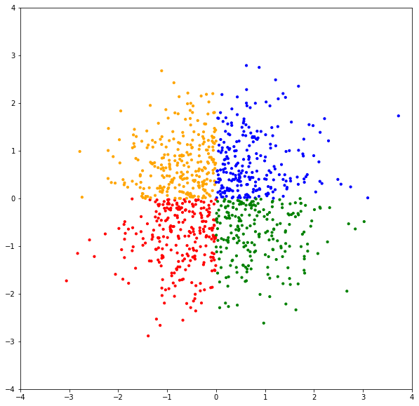
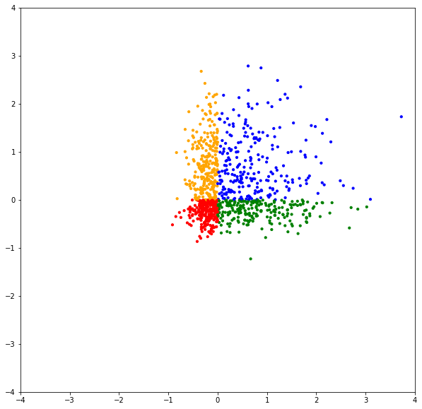
Figure 2: (a) Samples from of a Gaussian distribution with $\mu=[0,0]$ and $\Sigma=I$. The samples are colored according to the quadrant they belong to. (b) Samples from the distribuion in a) transformed by a PReLU transformation.

3

Figure 3: Samples from a Gaussian with $\mu=[0,0]$ and $\Sigma=I$, transformed by PReLU transformations with different $\alpha$ parameters. (a) $\alpha=0.1$ (b) $\alpha=0.5$ (c) $\alpha=5$

2.4.3 Batch-Normalization Transformation

[3] propose a batch-normalization transformation, similar to the well-known batch-normalization layer normally used in neural networks. This transform simply applies a rescaling, given the batch mean $\tilde{\mu}$ and variance ${\tilde{\sigma}}^{2}$:

$$f(z)=\frac{z-\tilde{\mu}}{\sqrt{{\tilde{\sigma}}^{2}+\epsilon}},$$ (17)

where $\epsilon\ll 1$ is a term used to ensure that there never is a division by zero. This transformation’s Jacobian is trivial:

$$\prod_{i=1}^{D}\frac{1}{\sqrt{{\tilde{\sigma}}_{i}^{2}+\epsilon}}.$$ (18)

2.4.4 Affine Coupling Transformation

As mentioned previously, one of the active research challenges within the normalizing flows framework is the search and design of transformations that are sufficiently expressive and whose Jacobians are not computationally heavy. One brilliant example of such transformations, proposed by [3], is called affine coupling layer.

This transformation is characterized by two arbitrary functions $s(.)$ and $t(.)$, as well as a mask that splits an input $\bm{z}$ of dimension $D$ into two parts, $\bm{z_{1}}$ and $\bm{z_{2}}$. In practice, $s(.)$ and $t(.)$ are neural networks, whose parameters are to be optimized so as to make the transformation approximate the desired output distribution. The outputs of $s(.)$ and $t(.)$ need to have the same dimension as $\bm{z_{1}}$. This should be taken into account when designing the mask and the functions $s(.)$ and $t(.)$. The transformation is defined as:

$$\begin{cases}\bm{x_{1}}&=\bm{z_{1}}\odot\exp\big{(}s(\bm{z_{2}})\big{)}+t(\bm{z_{2}})\\ \bm{x_{2}}&=\bm{z_{2}}.\end{cases}$$ (19)

To see why this transformation is suitable to being used within the framework of normalizing flows, let us derive its Jacobian.

• $\frac{\partial\bm{x_{2}}}{\partial\bm{z_{2}}}=I$, because $\bm{x_{2}}=\bm{z_{2}}$.

• $\frac{\partial\bm{x_{2}}}{\partial\bm{z_{1}}}$ is a matrix of zeros, because $\bm{x_{2}}$ does not depend on $\bm{z_{1}}$.

• $\frac{\partial\bm{x_{1}}}{\partial\bm{z_{1}}}$ is a diagonal matrix, whose diagonal is simply given by $\exp\big{(}s(\bm{z_{2}})\big{)}$, since those values are constant w.r.t $\bm{z_{1}}$ and they are multiplying each element of $\bm{z_{1}}$.

• $\frac{\partial\bm{x_{1}}}{\partial\bm{z_{2}}}$ is not needed, as will become clear ahead.

Writing the above in matrix form:

shows that the Jacobian matrix is (upper) triangular. Its determinant - the only thing we need, in fact - is therefore easy to compute: it is simply the product of the diagonal elements. Moreover, part of the diagonal is simply composed of ones. The determinant, and the log-absolute-determinant become

$$\det\big{(}J_{f(z)}\big{)} =\prod_{i}\exp\big{(}s(\bm{z_{2}}^{(i)})\big{)}$$ (24)

$$\log\Big{|}\det\big{(}J_{f(z)}\big{)}\Big{|} =\sum_{i}s(\bm{z_{2}}^{(i)}),$$ (25)

where $\bm{z_{2}^{(i)}}$ is the $i$-th element of $\bm{z_{2}}$. Since a single affine coupling layer does not transform all of the elements in $\bm{z}$, in practice several layers are composed, and each layer’s mask is changed so as to make all dimensions affect each other. This can be done, for instance, with a checkerboard pattern, which alternates for each layer. In the case of image inputs, the masks can operate at the channel level.

2.4.5 Masked Autoregressive Flows

Another ingenious architecture for normalizing flows has been proposed by [16]. It is called masked autoregressive flow (MAF). Let $\bm{z}$ be a sample from some base distribution, with dimension $D$. MAF transforms $\bm{z}$ into an observation $\bm{x}$, of the same dimension, in the following manner:

$$x_{i}=z_{i}\exp(\alpha_{i})+\mu_{i}$$ (26)

$$(\mu_{i},\alpha_{i})=g(\bm{x_{1:i-1}}).$$ (27)

In the above expression $g$ is some arbitrary function. The inverse transform of MAF is trivial, because, like the affine coupling layer, MAF uses $g$ to parameterize a shift, $\mu$, and a log-scale, $\alpha$, which translates to the fact that the function $g$ itself does not need to be inverted:

$$z_{i}=(x_{i}-\mu_{i})\exp(-\alpha_{i}).$$ (28)

Moreover, the autoregressive structure of the transformation constrains the Jacobian to be triangular, which renders the determinant effortless to compute:

$$\det\big{(}J_{f(\bm{z})}\big{)} =\prod_{i=1}^{D}\exp(\alpha_{i}),$$ (29)

$$\log\Big{|}\det\big{(}J_{f(\bm{z})}\big{)}\Big{|} =\sum_{i=1}^{D}\alpha_{i}.$$ (30)

As stated above, the function $g$ used to obtain $\mu_{i}$ and $\alpha_{i}$ can be arbitrary. However, in the original paper, the function proposed a masked autoencoder for distribution estimation (MADE), as described by [5].

Much like the partitioning in the affine coupling layer, the assumption of autoregressiveness (and the ordering of the elements of $\bm{x}$ for which that assumption is held) carries an inductive bias with it. Again, like with the affine coupling layer, this effect is minimized in practice by stacking layers with different element orderings.

2.5 Fitting Normalizing Flows

Generally speaking, normalizing flows can be used in one of two scenarios: (direct) density estimation, where the goal is to optimize the parameters so as to make the model approximate the distribution of some observed set of data; in a variational inference scenario, as way of having a flexible variational posterior. The second scenario is out of the scope of this work.

The task of density estimation with normalizing flows reduces to finding the optimal parameters of a parametric model. In general, there are two ways to go about estimating the parameters of a parametric model, given data: MLE and MAP. In the case of normalizing flows, MLE is the usual approach. To fit a normalizing flow via MLE, a gradient based optimizer is used to minimize $\hat{\mathcal{L}}(\bm{\theta})=-\mathbb{E}[\log p(\bm{x}|\bm{\theta})]$. However, this expectation is generally not accesible, since we have only finite samples of $\bm{x}$. Because of that, the parameters are estimated by optimizing an approximation of that expectation: $-\frac{1}{N}\sum_{i=1}^{N}\log p(\bm{x_{i}}|\bm{\theta})$.

To perform optimization on this objective, stochastic gradient descent (SGD) - and its variants - is the most commonly used algorithm. In general terms, SGD is an approximation of gradient descent, which rather than using the actual gradient, at time step $t$, to update the variables under optimization, works by computing several estimates of that gradient and using those estimates instead. This is done by partitioning the data in mini-batches, and computing the loss function and respective gradients over those mini-batches. This way, one pass through data - an epoch - results in several parameter updates.

3 Variational Mixture of Normalizing Flows

3.1 Introduction

The ability of leveraging domain knowledge to endow a probabilistic model with structure is often useful. The goal of this work is to devise a model that combines the flexibility of normalizing flows with the ability to exploit class-membership structure. This is achieved by learning a mixture of normalizing flows, via optimization of a variational objective, for which the variational posterior over the class-indexing latent variables is parameterized by a neural network. Intuitively, this neural network should learn to place similar instances of data in the same class, allowing each component of the mixture to be fitted to a cluster of data.

3.2 Model Definition

Let us define a mixture model, where each of the $K$ components is a density parameterized by a normalizing flow. For simplicity, consider that all of the $K$ normalizing flows have the same architecture, i.e., they are all composed of the same stack of transformations, but they each have their own parameters.

Additionally, let $q(z|\bm{x};\gamma)$ be a neural network with a $K$-class softmax output, with parameters $\bm{\gamma}$. This network will receive as input an instance from the data, and produce the probability of that instance belonging to each of the $K$ classes.

Recall the evidence lower bound (the dependence of $q$ on $x$ is made explicit):

$$\text{ELBO}=\mathbb{E}_{q}[\log p(\bm{x},z)]-\mathbb{E}_{q}[\log q(z|\bm{x})].$$

Let us rearrange it:

ELBO $$=\mathbb{E}_{q}[\log p(\bm{x}|z)]+\mathbb{E}_{q}[\log p(z)]-\mathbb{E}_{q}[\log q(z|\bm{x})]$$ (31)

$$=\mathbb{E}_{q}[\log p(\bm{x}|z)+\log p(z)-\log q(z|\bm{x})]$$ (32)

Since $q(z|\bm{x})$ is given by the forward-pass of a neural network, and is therefore straightforward to obtain, the expectation in (32) is given by computing the expression inside the expectation for each possible value of $z$, and summing the obtained values, weighed by the probabilities given by the variational posterior:

$$\text{ELBO}=\sum_{z=1}^{K}q(z|\bm{x})\big{(}\log p(\bm{x}|z)+\log p(z)-\log q(z|\bm{x})\big{)}.$$ (33)

Thus, the whole ELBO is easy to compute, provided that each of the terms inside the expectation is itself easy to compute. Let us consider each of those terms:

• $\log p(\bm{x}|z)$ is the log-likelihood of $\bm{x}$ under the normalizing flow indexed by $z$. It was shown in the previous section how to compute this.

• $\log p(z)$ is the log-prior of the component weights. For simplicity, let us assume this is set by the modeller. When nothing is known about the component weights, the best assumption is that they are uniform.

• $-\log q(z|\bm{x})$ is the negative logarithm of the output of the encoder.

Let us call this model variational mixture of normalizing flows (VMoNF). For an overview of the model, consider Figures 4 and 5

Figure 4: Plate diagram of a mixture of $K$ normalizing flows. $\bm{\theta}_{k}$ is the parameter vector of component $k$.

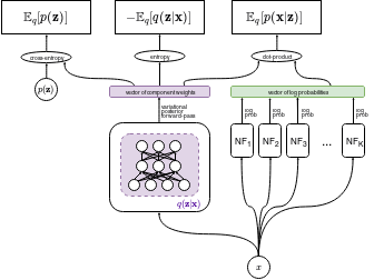
Figure 5: Overview of the training procedure of the VMoNF.

In a similar fashion to the variational auto-encoder, proposed by [13], a VMoNF is fitted by jointly optimizing the parameters of the variational posterior $q(z|\bm{x};\bm{\gamma})$ and the parameters of the generative process $p(\bm{x}|z;\bm{\theta})$. After training, the variational posterior naturally induces a clustering on the data, and can be directly used to assign new data points to the discovered clusters. Moreover, each of the fitted components can be used to generate samples from the cluster it “specialized” in.

3.3 Implementation

To implement and test the proposed model, Python was the chosen language. More specifically, this work heavily relies on the PyTorch [17] package and framework for automatic differentiation. Moreover, the parameter optimization is done via stochastic optimization, namely using the Adam optimizer, proposed by [11].

Figure 5 gives an overview of the training procedure:

1. The log-probabilities given by each component of the mixture are computed.

2. The values of the variational posterior probabilities for each component are computed.

3. With the results of the previous steps, all three terms of the ELBO are computable.

4. The ELBO and its gradients w.r.t the model parameters are computed and the parameters are updated.

5. Steps 1 to 4 are repeated until some stopping criterion is met.

4 Experiments

In this section, the proposed model is applied to two benchmark synthetic datasets (Pinwheel and Two-circles) and one real-world dataset (MNIST). On one of the synthetic datasets, one shortcoming of the model is brought to attention, but is overcome in a semi-supervised setting. On the real-world dataset, the model’s clustering capabilities are evaluted, as well as its capacity to model complex distributions.

A technique inspired in the work of [20] was employed to improve training speed and quality of results. This consists in dividing the inputs of the softmax layer in the variational posterior by a “temperature” value, $T$, which follows an exponential decay schedule during training. Intuitively, this makes the variational posterior “more certain” as training proceeds, while allowing all components to be generally exposed to the whole data, during the initial epochs. This discourages components from being “subtrained” during the initial epochs and, subsequently, from being prematurely discarded by the variational posterior.

4.1 Toy datasets

4.1.1 Pinwheel dataset

This dataset is constituted by five non-linear “wings”. See Figure 6 for the results of running the model on this dataset. As expected, the variational posterior has learned to partition the space so as to attribute each “wing” to a component of the mixture. This partitioning is imperfect in regions of space that have low probability for every component.

2

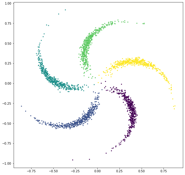
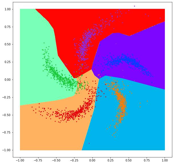
Figure 6: (a) Original dataset. (b) Samples from the learned model. Each dot is colored according to the component it was sampled from. The background colors denote the regions where each component has maximum probability assigned by the variational posterior. (Note that the background colors were chosen so as to not match the dot colors, otherwise the dots would not be visible)

This experiment consisted of training on 2560 data points (512 per class) using the Adam optimizer, with a learning rate of 0.001, a mini-batch size of 512, during 400 epochs. The variational posterior was parameterized by a multi-layer perceptron, with 1 hidden layer of dimension 3, and a softmax output. Each component of the mixture was a RealNVP with 8 blocks, each block with multi-layer perceptrons, with 1 hidden layer of dimension 8 as the $s(.)$ and $t(.)$ functions of the affine coupling layers.

4.1.2 Two-circles dataset

This dataset consists of two concentric circles. The experiment on this dataset, shown on Figure 7, makes evident one shortcoming of this model: the way in which the variational posterior partitions the space is not necessarily guided by the intrisic structure in the data. In the case of the two-circles dataset, it was found that the most common space partitioning induced by the model consisted simply of splitting into two half-spaces. However, in a semi-supervised setting, this behaviour can be corrected and the model successfully learns to separate the two circles, as shown in Figure 8. In this setting, the model was pretrained on the labeled instances for some epochs and then trained with the normal procedure. In the semi-supervised setting, the model has the chance to refine both the variational posterior and each of the components, thus making better use of the unlabeled data in the unsupervised phase of the training. As is clearly visible in Figure 8, the model struggles with learning full, closed, circles; this is because it is unable to “pierce a hole” in the base distribution, due to the nature of the transformations that are applicable. Thus, to model a circle, the model has to learn to stretch the blob formed by the base distribution, and “bend it over itself”. This difficulty is also what keeps the model from learning a structurally interesting solution in the fully unsupervised case: it is easier to learn to distort space so as to learn a multimodal distribution that models half of the two circles. Moreover, the points in diametrically opposed regions of the same circle are more dissimilar (in the geometrical sense) than points in the same region of the two circles. Therefore, when completely uninformed by labels, the variational posterior’s layers will tend to have similar activations for points in the latter case, and thus tend to place them in the same class.

The unsupervised learning experiment consisted of training on 1024 datapoints, 512 per class; using the Adam optimizer, with a learning rate of 0.001, a mini-batch size of 128, during 500 epochs. The semi-supervised learning experiment consisted of training on 1024 unlabeled datapoints, 512 per class and 64 labeled data points, 32 per class. The model was first pretrained during 300 epochs solely on the 32 labeled data points, using the labels to selectively optimize each component of the mixture, as well as to optimize the variational posterior by minimizing a binary cross-entropy loss. After pretraining, the model was trained by interweaving supervised epochs - like in pretraining - with unsupervised epochs. Optimization was carried out using the Adam optimizer, with a learning rate of 0.001, a mini-batch size of 128, during 500 epochs. For both the unsupervised and the semi-supervised experiments, the neural network used to parameterize the variational posterior was a multi-layer perceptron, with 2 hidden layers of dimension 16, and with a softmax output. Each component of the mixture was a RealNVP with 10 blocks, each block with multi-layer perceptrons, with 1 hidden layer of dimension 8, as the $s(.)$ and $t(.)$ functions of the affine coupling layers.

2

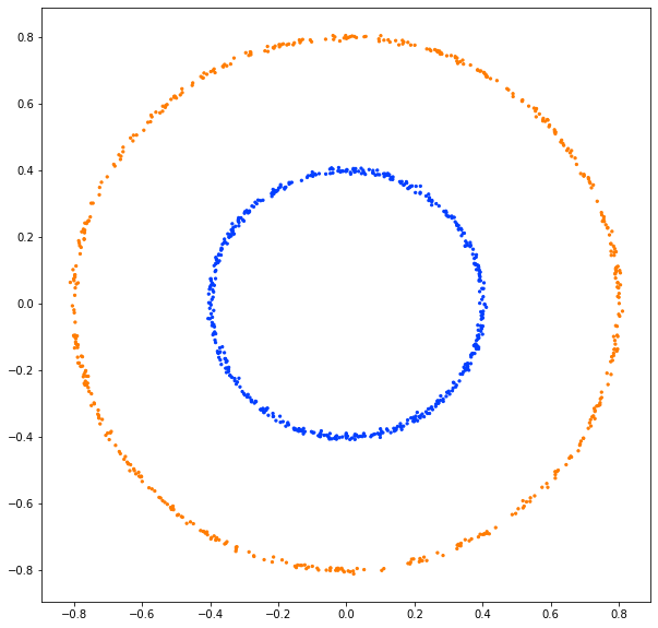
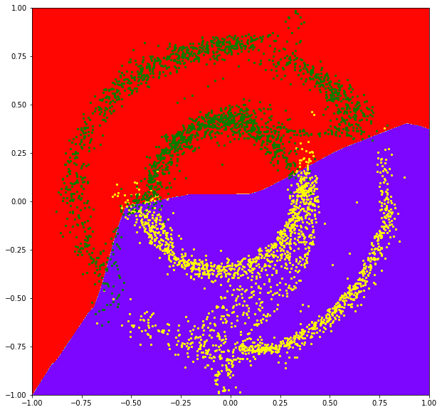
Figure 7: (a) Original dataset. (b) Samples from the learned model, without any labels. Coloring logic is the same as in 6.

2

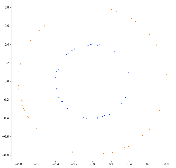
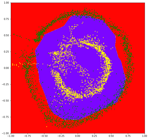
Figure 8: (a) Labeled points used in semi-supervised scenario. (b) Samples from the model trained in the semi-supervised scenario.

4.2 Real-world dataset

In this subsection, the proposed model is evaluated on the well-known MNIST dataset [14]. This dataset consists of images of handwritten digits. The grids are of dimension 28 x 28 and were flattened to vectors of dimension 784 for training. For this experiment, only the images corresponding to the digits from 0 to 4 were considered. The normalizing flow model used for the components was a MAF, with 5 blocks, whose internal MADE layers had 1 hidden layer of dimension 200. The variational posterior was parameterized by a multi-layer perceptron, with 1 hidden layer of dimension 512. The model was trained for 100 epochs, with a mini-batch size of 100. The Adam optimizer was used, with a learning rate of 0.0001, and with a weight decay parameter of 0.000001. In Figure 9, samples from the components obtained after training can be seen. Moreover, a normalized contingency table is presented, where the performance of the variational posterior as a clustering function can be assessed. Note that the cluster indices induced by the model have no semantic meaning.

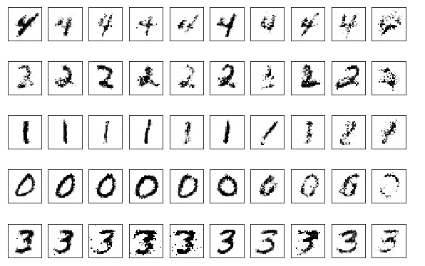
Figure 9: Samples from the fitted mixture components. Each row is sampled from the same component

	0	1	2	3	4
0	0.000602	0.012432	0.002807	0.982555	0.001604
1	0.002139	0.020146	0.977001	0.000178	0.000535
2	0.000802	0.952276	0.011630	0.007219	0.028073
3	0.001558	0.479455	0.300682	0.004284	0.214021
4	0.646166	0.347273	0.005125	0.001435	0.000000

Table 1: Normalized contingency table for the clustering induced by the model

From Table 1 and Figure 9 it is possible to see that although there is some confusion, the model successfully clusters the MNIST digits.

5 Conclusions

5.1 Conclusions

Deep generative modelling is an active research avenue that will keep being developed and improved, since it lends itself to extremely useful applications, like anomaly detection, synthetic data generation, and, generally speaking, uncovering patterns in data. Overall, the initial idea of the present work stands validated by the experiments - it is possible to learn mixtures of normalizing flows via the proposed procedure - as well as by recently published similar work RADsemisuplearning_nflows. The proposed method was tested on two synthetic datasets, succeeding with ease on one of them, and struggling with the other one. However, when allowed to learn from just a few labels, it was able to successfully fit the data it previously failed on. On the real-world dataset, the model’s clustering capability was tested, as well as its ability to generate realistic samples, with some success. During the experiments, it became evident that, similarly to what happens with the majority of neural-network-based models, in order to successfully fit the proposed model to complex data, some fine tuning is required, both in terms of the training procedure, as well as in terms of the architecture of the blocks that constitute the model. In the following subsection, some proposals and ideas for future work and for tackling some of the observed shortcomings are proposed.

5.2 Discussion and Future Work

After the work presented here, some observations and future research questions and ideas arise:

• The main shortcoming of the proposed model, specially in its fully unsupervised variant, is that there is no way to incentivize the variational posterior to partition the space in the intuitively correct manner. Moreover, the variational posterior generally performs poorly in regions of space where there are few or no training points. This suggests that the model could benefit from a consistency loss regularization term. In fact, this idea has been pursued by [9].

• Some form of weight-sharing strategy between components is also an interesting point for future research. It is plausible that, this way, components could share “concepts” and latent representations of data, and use their non-shared weights to “specialize” in their particular cluster of data. Take, for instance, the Pinwheel dataset: in principle, the five normalizing flows could share a stack of layers that learned to model the concept of wing, each component then having a non-shared stack of blocks that would only need to model the correct rotation of its respective wing.

• During the experimentation phase, it was found that a balance between the complexity of the variational posterior and that of the components of the mixture, is crucial for the convergence to interesting solutions. This is intuitive: if the components are too complex, the variational posterior tends to ignore most of them and assigns most points to a single or few components.

• The fact that in some cases the variational posterior ignores components and “chooses” not to use them can hypothetically be exploited in the scenarios where the number of clusters is unknown. If the dynamics of what drives the variational posterior to ignore components can be understood, perhaps they can be actively tweaked (via architectural choices, training procedure and hyperparameters, for example) to benefit the modelling task in such a scenario.

• Related to the previous point, one first experiment could be to update the prior ($p(z)$) (for example, every epoch), based on the responsabilities given by the variational posterior.

• The effect of using different architectures for the neural networks used was not evaluated. It is likely, for instance, that convolutional architectures would produce better results in the real world dataset.

References

- [1] Nicola De Cao, Ivan Titov and Wilker Aziz “Block Neural Autoregressive Flow” In 35th Conference on Uncertainty in Artificial Intelligence (UAI19), 2019
- [2] Nat Dilokthanakul et al. “Deep Unsupervised Clustering with Gaussian Mixture Variational Autoencoders”, 2016 eprint: arXiv:1611.02648
- [3] Laurent Dinh, Jascha Sohl-Dickstein and Samy Bengio “Density estimation using Real NVP” In 5th International Conference on Learning Representations, ICLR 2017, Toulon, France, April 24-26, 2017, Conference Track Proceedings, 2017
- [4] Laurent Dinh, Jascha Sohl-Dickstein, Razvan Pascanu and Hugo Larochelle “A RAD approach to deep mixture models”, 2019 eprint: arXiv:1903.07714
- [5] Mathieu Germain, Karol Gregor, Iain Murray and Hugo Larochelle “MADE: Masked Autoencoder for Distribution Estimation” In Proceedings of the 32nd International Conference on Machine Learning 37, Proceedings of Machine Learning Research Lille, France: PMLR, 2015, pp. 881–889 URL: http://proceedings.mlr.press/v37/germain15.html
- [6] Ian Goodfellow et al. “Generative Adversarial Nets” In Advances in Neural Information Processing Systems 27 Curran Associates, Inc., 2014, pp. 2672–2680
- [7] Aditya Grover, Manik Dhar and Stefano Ermon “Flow-GAN: Combining Maximum Likelihood and Adversarial Learning in Generative Models” In AAAI Conference on Artificial Intelligence, 2018
- [8] Jonathan Ho et al. “Flow++: Improving Flow-Based Generative Models with Variational Dequantization and Architecture Design” In Proceedings of the 36th International Conference on Machine Learning 97, Proceedings of Machine Learning Research Long Beach, California, USA: PMLR, 2019, pp. 2722–2730 URL: http://proceedings.mlr.press/v97/ho19a.html
- [9] Pavel Izmailov, Polina Kirichenko, Marc Finzi and Andrew Gordon Wilson “Semi-Supervised Learning with Normalizing Flows” In Workshop on Invertible Neural Networks and Normalizing Flows, 2019
- [10] M. Johnson et al. “Composing graphical models with neural networks for structured representations and fast inference” In Advances in Neural Information Processing Systems 29 Curran Associates, Inc., 2016, pp. 2946–2954
- [11] Diederik P Kingma and Jimmy Ba “Adam: A method for stochastic optimization” In International Conference on Learning Representations (ICLR), 2015
- [12] Diederik P Kingma and Prafulla Dhariwal “Glow: Generative Flow with Invertible 1x1 Convolutions” In Advances in Neural Information Processing Systems 31 Curran Associates, Inc., 2018, pp. 10215–10224
- [13] Diederik P Kingma and Max Welling “Auto-encoding variational Bayes” In International Conference on Learning Representations (ICLR), 2014
- [14] Yann LeCun and Corinna Cortes “MNIST handwritten digit database”, http://yann.lecun.com/exdb/mnist/, 2010 URL: http://yann.lecun.com/exdb/mnist/
- [15] Wu Lin, Mohammad Emtiyaz Khan and Nicolas Hubacher “Variational Message Passing with Structured Inference Networks” In International Conference on Learning Representations, 2018
- [16] George Papamakarios, Theo Pavlakou and Iain Murray “Masked Autoregressive Flow for Density Estimation” In Advances in Neural Information Processing Systems 30 Curran Associates, Inc., 2017, pp. 2338–2347 URL: http://papers.nips.cc/paper/6828-masked-autoregressive-flow-for-density-estimation.pdf
- [17] Adam Paszke et al. “Automatic Differentiation in PyTorch” In NIPS Autodiff Workshop, 2017
- [18] Danilo Rezende and Shakir Mohamed “Variational Inference with Normalizing Flows” In Proceedings of the 32nd International Conference on Machine Learning 37, Proceedings of Machine Learning Research Lille, France: PMLR, 2015, pp. 1530–1538
- [19] Junyuan Xie, Ross Girshick and Ali Farhadi “Unsupervised Deep Embedding for Clustering Analysis” In Proceedings of The 33rd International Conference on Machine Learning 48, Proceedings of Machine Learning Research New York, New York, USA: PMLR, 2016, pp. 478–487
- [20] Dejiao Zhang, Yifan Sun, Brian Eriksson and Laura Balzano “Deep Unsupervised Clustering Using Mixture of Autoencoders”, 2017 eprint: arXiv:1712.07788