Conjectures on spectral properties of ALIF algorithm

Abstract

A new decomposition method for nonstationary signals, named Adaptive Local Iterative Filtering (ALIF), has been recently proposed in the literature. Given its similarity with the Empirical Mode Decomposition (EMD) and its more rigorous mathematical structure, which makes feasible to study its convergence compared to EMD, ALIF has really good potentiality to become a reference method in the analysis of signals containing strong nonstationary components, like chirps, multipaths and whistles, in many applications, like Physics, Engineering, Medicine and Finance, to name a few.

In [11], the authors analyzed the spectral properties of the matrices produced by the ALIF method, in order to study its stability. Various results are achieved in that work through the use of Generalized Locally Toeplitz (GLT) sequences theory, a powerful tool originally designed to extract information on the asymptotic behavior of the spectra for PDE discretization matrices. In this manuscript we focus on answering some of the open questions contained in [11], and in doing so, we also develop new theory and results for the GLT sequences.

Mathematics Subject Classification: 94A12, 68W40, 15A18, 47B06, 15B05

Index terms— iterative filtering, adaptive local iterative filtering, empirical mode decomposition, convergence analysis, eigenvalue distribution, generalized locally Toeplitz sequences, nonostationary signals, signal decomposition

1 Introduction

The decomposition and subsequent time–frequency analysis of nonstationary signals is an important topic of research which received a significant acceleration from the publication of the seminal work on the Empirical Mode Decomposition (EMD) method by Huang et al. [27] in 1998. In particular, Huang and his collegues at NASA proposed to iteratively decompose a given signal into a finite number of “simple components” called Intrinsic Mode Functions (IMFs) which fulfil the following two properties:

• the number of zero crossings and the number of extrema must be either equal or differ at most by one;

• at any point, the mean value of the envelope connecting the local maxima and the envelope connecting the local minima must be zero.

The decompositions produced using the EMD algorithm attracted the interest of a high number of researchers and it proved to be successful for a wide range of applications, as testified by the number of citations, more than 14600, that the paper [27] by itself has received so far. Nevertheless, the EMD algorithm is based on the iterative calculation of envelopes which are taylored on the specific signal under study. This makes really hard to analyze the EMD mathematically. Furthermore, this approach has also stability problems in the presence of noise, as illustrated in [46]. Several variants of the EMD have been recently proposed to address this last problem, e.g. the Ensemble Empirical Mode Decomposition (EEMD) [46], the complementary EEMD [48], the complete EEMD [44], the partly EEMD [51], the noise assisted multivariate EMD (NA-MEMD) [45]. They all allow to address the EMD stability issue as well as to reduce the so called mode mixing problem [51]. But their mathematical understanding, like the EMD one, is far from be complete. Furthermore, from the prospective of nonstationarities handling, they pose new challenges since they worsen the mode–splitting problem present in the EMD algorithm [48]. Over the years many alternative approaches to the EMD have been proposed, like, for instance, the sparse TF representation [24, 25], the Geometric mode decomposition [49], the Empirical wavelet transform [23], the Variational mode decomposition [19], and similar techniques [38, 32, 37]. All these methods are based on optimization with respect to an a priori chosen basis. The only alternative method proposed so far in the literature which is based on iterations, and hence does not require any a priori assumption on the signal under analysis, is named Iterative Filtering [30, 7, 12]. This alternative iterative method, although published only recently, has already been used effectively in a wide variety of applied fields, like, for instance, in [50, 2, 3, 5, 13, 1, 4, 28, 47, 14, 36, 40, 33, 29, 31, 39, 41, 42, 34, 35, 22, 21]. The IF algorithm structure resembles the EMD one. Its key difference is in the way the signal moving average is computed, i.e., via correlation of the signal with an a priori chosen filter function, whereas, in the EMD–based methods, it is computed as average between two envelopes. This apparently simple difference opens the doors to a complete mathematical analysis of the IF method [26, 12, 16, 9, 8, 10, 17, 18, 43]. The only problem in the IF method is its limitation in the variability of the instantaneous frequency of each single IMF component. This becomes an issue when we are dealing with signals which contain strong nonstationarities, like the so called chirps and whistles. This is the mode–splitting problem which effects also EMD and derived algorithms [48]. To solve this problem, the Adaptive Local Iterative Filtering (ALIF) algorithm has been recently proposed in [12]. ALIF is a flexible generalization of IF which completely overcome the limitations of the IF method by computing wisely chosen local and adaptive signal averages. This makes ALIF algorithm an extremely promising and unique technique for the extraction of chirps from nonstationary signals. However, the ALIF convergence cannot be guaranteed a priori yet. Some advances have been recently achieved in the literature [11, 15], but the main questions are still open. In particular in [11] the authors propose two conjectures which we discuss thoroughly in this work.

The rest of this work is organized as follows. In Section 2 we recall all the basic mathematical tools required to analyze the ALIF iteration matrix asymptotic spectral properties. In Section 3 we recall the ALIF methods and the conjectures originally proposed in [11]. Sections 4 and 5 are devoted to the analysis of the two conjectures, for which we need some technical and auxiliary results reported and proved in the appendix. In particular, Appendix A contains some novel contributions to the theory of GLT sequences and spectral symbols.

2 Spectral analysis tools

We present in this section the tools for analyzing the asymptotic spectral properties of the ALIF iteration matrix. Throughout this paper, a matrix-sequence is any sequence of the form $\{A_{n}\}_{n}$, where $A_{n}$ is a square matrix of size $n$.

If $A$ is an $n\times n$ matrix and $1\leq p\leq\infty$, we denote by $\|A\|_{p}$ the Schatten $p$-norm of $A$, i.e., the $p$-norm of the vector $(\sigma_{1}(A),\ldots,\sigma_{n}(A))$ formed by the singular values of $A$. The Schatten $\infty$-norm $\|A\|_{\infty}$ is the largest singular value of $A$ and coincides with the spectral norm $\|A\|$. The Schatten 2-norm $\|A\|_{2}$ coincides with the Frobenius norm, i.e., $\|A\|_{2}=(\sum_{i,j=1}^{n}|a_{ij}|^{2})^{1/2}$.

2.1 Singular value and eigenvalue distribution of a matrix-sequence

Let $C_{c}(\mathbb{C})$ be the space of continuous complex-valued functions with bounded support defined on $\mathbb{C}$ and let $\mu_{p}$ be the Lebesgue measure in $\mathbb{R}^{p}$. If $A$ is a square matrix of size $n$, the singular values and the eigenvalues of $A$ are denoted by $\sigma_{1}(A),\ldots,\sigma_{n}(A)$ and $\lambda_{1}(A),\ldots,\lambda_{n}(A)$, respectively.

Definition 1

Let $\{A_{n}\}_{n}$ be a matrix-sequence and let $f:D\subset\mathbb{R}^{p}\to\mathbb{C}$ be a measurable function defined on a set $D$ with $0<\mu_{p}(D)<\infty$.

• We say that $\{A_{n}\}_{n}$ has a singular value distribution described by $f$, and we write $\{A_{n}\}_{n}\sim_{\sigma}f$, if for all $F\in C_{c}(\mathbb{C})$ we have

  $$\lim_{n\to\infty}\frac{1}{n}\sum_{i=1}^{n}F(\sigma_{i}(A_{n}))=\frac{1}{\mu_{p}(D)}\int_{D}F(|f(y_{1},\ldots,y_{p})|){\rm d}y_{1}\ldots{\rm d}y_{p}.$$

• We say that $\{A_{n}\}_{n}$ has an eigenvalue distribution described by $f$, and we write $\{A_{n}\}_{n}\sim_{\lambda}f$, if for all $F\in C_{c}(\mathbb{C})$ we have

  $$\lim_{n\to\infty}\frac{1}{n}\sum_{i=1}^{n}F(\lambda_{i}(A_{n}))=\frac{1}{\mu_{p}(D)}\int_{D}F(f(y_{1},\ldots,y_{p})){\rm d}y_{1}\ldots{\rm d}y_{p}.$$

If $\{A_{n}\}_{n}$ has both a singular value and an eigenvalue distribution described by $f$, we write $\{A_{n}\}_{n}\sim_{\sigma,\lambda}f$.

2.2 Informal meaning of the singular value and eigenvalue distribution

Assuming $f$ is Riemann-integrable, the eigenvalue distribution $\{A_{n}\}_{n}\sim_{\lambda}f$ has the following informal meaning [20, Section 3.1]: all the eigenvalues of $A_{n}$, except possibly for $o(n)$ outliers, are approximately equal to the samples of $f$ over a uniform grid in $D$ (for $n$ large enough). For instance, if $p=1$ and $D=[a,b]$, then, assuming we have no outliers, the eigenvalues of $A_{n}$ are approximately equal to

$$f\Bigl{(}a+i\,\frac{b-a}{n}\Bigr{)},\quad i=1,\ldots,n,$$

for $n$ large enough. Similarly, if $p=2$, $n=m^{2}$ and $D=[a_{1},b_{1}]\times[a_{2},b_{2}]$, then, assuming we have no outliers, the eigenvalues of $A_{n}$ are approximately equal to

$$f\Bigl{(}a_{1}+i\,\frac{b_{1}-a_{1}}{m},\,\,a_{2}+j\,\frac{b_{2}-a_{2}}{m}\Bigr{)},\quad i,j=1,\ldots,m,$$

for $n$ large enough. A completely analogous meaning can also be given for the singular value distribution $\{A_{n}\}_{n}\sim_{\sigma}f$.

2.3 Zero-distributed sequences

A matrix-sequence $\{Z_{n}\}_{n}$ such that $\{Z_{n}\}_{n}\sim_{\sigma}0$ is referred to as a zero-distributed sequence. In other words, $\{Z_{n}\}_{n}$ is zero-distributed if and only if $\lim_{n\to\infty}\frac{1}{n}\sum_{i=1}^{n}F(\sigma_{i}(Z_{n}))=F(0)$ for all $F\in C_{c}(\mathbb{C})$. Proposition 1 is proved in [20, Section 3.4] and provides an important characterization of zero-distributed sequences together with a useful sufficient condition for detecting such sequences. For convenience, throughout this paper we use the natural convention $1/\infty=0$.

Proposition 1

Let $\{Z_{n}\}_{n}$ be a matrix-sequence.

• $\{Z_{n}\}_{n}$ is zero-distributed if and only if $Z_{n}=R_{n}+N_{n}$ with

  $$\lim_{n\to\infty}n^{-1}{\rm rank}(R_{n})=\lim_{n\to\infty}\|N_{n}\|=0.$$

• $\{Z_{n}\}_{n}$ is zero-distributed if there is a $p\in[1,\infty]$ such that

  $$\lim_{n\to\infty}n^{-1/p}\|Z_{n}\|_{p}=0.$$

2.4 Sequences of diagonal sampling matrices

If $n\in\mathbb{N}$ and $a:[0,1]\to\mathbb{C}$, the $n$th diagonal sampling matrix generated by $a$ is the $n\times n$ diagonal matrix given by

$$D_{n}(a)=\mathop{\rm diag}_{i=1,\ldots,n}a\Bigl{(}\frac{i}{n}\Bigr{)}.$$

$\{D_{n}(a)\}_{n}$ is called the sequence of diagonal sampling matrices generated by $a$.

2.5 Toeplitz sequences

If $n\in\mathbb{N}$ and $f:[-\pi,\pi]\to\mathbb{C}$ is a function in $L^{1}([-\pi,\pi])$, the $n$th Toeplitz matrix generated by $f$ is the $n\times n$ matrix

$$T_{n}(f)=[\hat{f}_{i-j}]_{i,j=1}^{n}=\begin{bmatrix}\hat{f}_{0}&\hat{f}_{-1}&\ \hat{f}_{-2}&\ \cdots&\ \ \cdots&\hat{f}_{-(n-1)}\\ \hat{f}_{1}&\ddots&\ \ddots&\ \ddots&\ \ &\vdots\\ \hat{f}_{2}&\ddots&\ \ddots&\ \ddots&\ \ \ddots&\vdots\\ \vdots&\ddots&\ \ddots&\ \ddots&\ \ \ddots&\hat{f}_{-2}\\ \vdots&&\ \ddots&\ \ddots&\ \ \ddots&\hat{f}_{-1}\\ \hat{f}_{n-1}&\cdots&\ \cdots&\ \hat{f}_{2}&\ \ \hat{f}_{1}&\hat{f}_{0}\end{bmatrix},$$

where the numbers $\hat{f}_{k}$ are the Fourier coefficients of $f$,

$$\hat{f}_{k}=\frac{1}{2\pi}\int_{-\pi}^{\pi}f(\theta){\rm e}^{-{\rm i}k\theta}{\rm d}\theta,\quad k\in\mathbb{Z}.$$

$\{T_{n}(f)\}_{n}$ is called the Toeplitz sequence generated by $f$.

2.6 Approximating classes of sequences

The notion of approximating classes of sequences (a.c.s.) is fundamental to the theory of Generalized Locally Toeplitz (GLT) sequences and it is deeply studied in [20, Chapter 5].

Definition 2

Let $\{A_{n}\}_{n}$ be a matrix-sequence and let $\{\{B_{n,m}\}_{n}\}_{m}$ be a sequence of matrix-sequences. We say that $\{\{B_{n,m}\}_{n}\}_{m}$ is an approximating class of sequences (a.c.s.) for $\{A_{n}\}_{n}$ if the following condition is met: for every $m$ there exists $n_{m}$ such that, for $n\geq n_{m}$,

$$A_{n}=B_{n,m}+R_{n,m}+N_{n,m},\quad{\rm rank}(R_{n,m})\leq c(m)n,\quad\|N_{n,m}\|\leq\omega(m),$$

where $n_{m},\,c(m),\,\omega(m)$ depend only on $m$, and $\displaystyle\lim_{m\to\infty}c(m)=\lim_{m\to\infty}\omega(m)=0$.

Roughly speaking, $\{\{B_{n,m}\}_{n}\}_{m}$ is an a.c.s. for $\{A_{n}\}_{n}$ if, for large $m$, the sequence $\{B_{n,m}\}_{n}$ approximates $\{A_{n}\}_{n}$ in the sense that $A_{n}$ is eventually equal to $B_{n,m}$ plus a small-rank matrix (with respect to the matrix size $n$) plus a small-norm matrix. We will use the convergence notation $\{B_{n,m}\}_{n}\stackrel{{\scriptstyle\rm a.c.s.}}{{\longrightarrow}}\{A_{n}\}_{n}$ to indicate that $\{\{B_{n,m}\}_{n}\}_{m}$ is an a.c.s. for $\{A_{n}\}_{n}$. A useful criterion to test the a.c.s. convergence is provided in the next theorem [20, Corollary 5.3].

Theorem 2.1

Let $\{A_{n}\}_{n},\{B_{n,m}\}_{n}$ be sequences of matrices, with $A_{n},B_{n,m}$ of size $n$, and let $1\leq p<\infty$. Suppose that for every $m$ there exists $n_{m}$ such that, for $n\geq n_{m}$,

$$\|A_{n}-B_{n,m}\|_{p}^{p}\leq\varepsilon(m,n)n,$$

where $\displaystyle\lim_{m\to\infty}\limsup_{n\to\infty}\varepsilon(m,n)=0$. Then $\{B_{n,m}\}_{n}\stackrel{{\scriptstyle\rm a.c.s.}}{{\longrightarrow}}\{A_{n}\}_{n}.$

2.7 GLT sequences

A GLT sequence $\{A_{n}\}_{n}$ is a special matrix-sequence equipped with a measurable function $\kappa:[0,1]\times[-\pi,\pi]\to\mathbb{C}$, the so-called symbol (or kernel). We use the notation $\{A_{n}\}_{n}\sim_{\rm GLT}\kappa$ to indicate that $\{A_{n}\}_{n}$ is a GLT sequence with symbol $\kappa$. The properties of GLT sequences that we shall need in this paper are listed below; the corresponding proofs can be found in [6, 20].

1. If $\{A_{n}\}_{n}\sim_{\rm GLT}\kappa$ then $\{A_{n}\}_{n}\sim_{\sigma}\kappa$. If $\{A_{n}\}_{n}\sim_{\rm GLT}\kappa$ and the matrices $A_{n}$ are Hermitian then $\{A_{n}\}_{n}\sim_{\lambda}\kappa$.

2. If $\{A_{n}\}_{n}\sim_{\rm GLT}\kappa$ and $A_{n}=X_{n}+Y_{n}$, where

   • every $X_{n}$ is Hermitian,

   • $n^{-1/2}\|Y_{n}\|_{2}\to 0$,

   then $\{A_{n}\}_{n}\sim_{\lambda}\kappa$.

3. We have

   • $\{T_{n}(f)\}_{n}\sim_{\rm GLT}\kappa(x,\theta)=f(\theta)$ if $f\in L^{1}([-\pi,\pi])$,

   • $\{D_{n}(a)\}_{n}\sim_{\rm GLT}\kappa(x,\theta)=a(x)$ if $a:[0,1]\to\mathbb{C}$ is Riemann-integrable,

   • $\{Z_{n}\}_{n}\sim_{\rm GLT}\kappa(x,\theta)=0$ if and only if $\{Z_{n}\}_{n}\sim_{\sigma}0$.

4. If $\{A_{n}\}_{n}\sim_{\rm GLT}\kappa$ and $\{B_{n}\}_{n}\sim_{\rm GLT}\xi$ then

   • $\{A_{n}^{*}\}_{n}\sim_{\rm GLT}\overline{\kappa}$,

   • $\{\alpha A_{n}+\beta B_{n}\}_{n}\sim_{\rm GLT}\alpha\kappa+\beta\xi$ for all $\alpha,\beta\in\mathbb{C}$,

   • $\{A_{n}B_{n}\}_{n}\sim_{\rm GLT}\kappa\xi$.

5. $\{A_{n}\}_{n}\sim_{\rm GLT}\kappa$ if and only if there exist GLT sequences $\{B_{n,m}\}_{n}\sim_{\rm GLT}\kappa_{m}$ such that $\{B_{n,m}\}_{n}\stackrel{{\scriptstyle\rm a.c.s.}}{{\longrightarrow}}\{A_{n}\}_{n}$ and $\kappa_{m}\to\kappa$ in measure over $[0,1]\times[-\pi,\pi]$.

If $\{A_{n}\}_{n}$ has singular value, eigenvalue distribution and GLT symbol described by a single function $\kappa$, we write $\{A_{n}\}_{n}\sim_{GLT,\sigma,\lambda}\kappa$.

3 The ALIF method

3.1 Terminology

Throughout this paper, any real function $g:\mathbb{R}\to\mathbb{R}$ is also referred to as a signal. Without loss of generality, we assume that the domain on which every signal $g$ is studied is the reference interval $[0,1]$. Outside the reference interval, the signal is usually not known and so, whenever necessary, we have to make assumptions, that is, we have to impose boundary conditions. The extrema of a signal $g$ are the points belonging to $(0,1)$ where $g$ attains its local maxima and minima. If $\mathbf{g}=[\mathbf{g}_{0},\ldots,\mathbf{g}_{n-1}]$ is a vector in $\mathbb{R}^{n}$, the extrema of $\mathbf{g}$ are the indices belonging to $\{1,\ldots,n-2\}$ where $\mathbf{g}$ attains its local maxima and minima, i.e., the indices $j\in\{1,\ldots,n-2\}$ such that $\mathbf{g}_{j}>\max(\mathbf{g}_{j-1},\mathbf{g}_{j+1})$ or $\mathbf{g}_{j}<\min(\mathbf{g}_{j-1},\mathbf{g}_{j+1})$. A filter $k$ is an even, nonnegative, bounded, measurable, and compactly supported function from $\mathbb{R}$ to $\mathbb{R}$ satisfying the normalization condition $\int_{\mathbb{R}}k(y){\rm d}y=1$. We refer to $\ell=\sup\{y>0:\,k(y)>0\}$ as the length of the filter $k$. Note that $0<\ell<\infty$ and the support of $k$ is contained in $[-\ell,\ell]$.

3.2 The ALIF method

Algorithm 1 (ALIF Algorithm) ${\rm IMFs=ALIF}(g)$

  IMFs = $\left\{\right\}$

  initialize the remaining signal $r=g$

  while the number of extrema of $r$ is $\geq 2$ do

     for each $x\in[0,1]$ compute the filter $k_{x}$, whose length $\ell(x)$ changes from $x$ to $x$ based on $r$ itself

     $g_{1}=r$

     $m=1$

     while the stopping criterion is not satisfied do

        compute the moving average $f_{m}$ of the signal $g_{m}$ as$f_{m}(x)=\int_{\mathbb{R}}g_{m}(y)k_{x}(x-y){\rm d}y$

        $g_{m+1}=g_{m}-f_{m}$

        $m=m+1$

     end while

     ${\rm IMFs}={\rm IMFs}\cup\{g_{m}\}$

     $r=r-g_{m}$

  end while

As mentioned in Section 1, the ALIF method is an iterative procedure whose purpose is to decompose a signal $g$ into a finite number of “simple components”, the so-called IMFs of $g$. Algorithm 1 shows the pseudocode of the ALIF method, in which the input is a signal $g$ and the output is the set of the IMFs of $g$. The ALIF algorithm contains two loops. The inner loop captures a single IMF, while the outer loop produces all the IMFs embedded in $g$. Considering the first iteration of the ALIF outer loop in which $g_{1}=g$, we see that the key idea to extract the first IMF consists in computing the moving average of $g_{m}$ and subtract it from $g_{m}$ itself so as to capture the fluctuation part $\mathcal{S}_{m}(g_{m})=g_{m}-f_{m}=g_{m+1}$. This is repeated iteratively and, assuming convergence, the first IMF is obtained as ${\rm IMF}_{1}=\lim_{m\to\infty}\mathcal{S}(g_{m})$. In practice, however, we cannot let $m$ go to $\infty$ and we have to use a stopping criterion, as indicated in Algorithm 1. Assuming convergence, one can stop the inner loop at the first index $m$ such that the difference $g_{m+1}-g_{m}$ is small in some norm (possibly, a norm for which the convergence is known). A safer stopping criterion also imposes a limit on the maximum number of iterations. This method of IMF extraction is shared with the EMD and IF algorithms and the only difference consists in the computation of the moving average. In the ALIF method, it is computed through the convolution with a filter $k_{x}$, that can depend on the point $x$. In practical applications of the ALIF method, first a length function $\ell(x)$ is computed based on the signal $g_{1}$, and then $k_{x}$ is chosen as 

$$k_{x}(y)=\frac{k\bigl{(}\frac{y}{\ell(x)}\bigr{)}}{\ell(x)},$$ (1)

where $k$ is an a priori fixed filter with length $1$, so that the length of $k_{x}$ is $\ell(x)$. Once the first IMF is obtained, to produce the second IMF we apply the previous process to the remaining signal $r=g-{\rm IMF}_{1}$. We then iterate this procedure to obtain all the IMFs of $g$, and we stop as soon as the remaining signal becomes a trend signal, meaning that it possesses at most one extremum. Clearly, the sum of all the IMFs of $g$ produced by the ALIF method with the final trend signal $r$ is equal to $g$.

Remark 1

In the case where $\ell(x)$ is chosen at each iteration of the outer loop as a constant $\ell$, depending on the remaining signal $r$ but not on $x$, the ALIF method reduces to the IF method, whose convergence has been studied in [11, 26].

3.3 The Discrete ALIF method

In practice, we usually do not know a signal $g$ on the whole reference interval $[0,1]$. What we actually know are the samples of $g$ over a fine grid in $[0,1]$. We therefore need a discrete version of the ALIF algorithm, which is able to (approximately) capture the IMFs of $g$ by exploiting this sole information. From now on, we make the following assumptions.

• For any signal $g$, no other information about $g$ is available except for its samples at the $n$ points $x_{i}=\frac{i}{n-1}$, $i=0,\ldots,n-1$. Moreover, $g=0$ outside $[0,1]$ (so we are imposing homogeneous Dirichlet boundary conditions).

• The filter $k_{x}$ is defined as in (1) in terms of an a priori fixed filter $k$ with length 1.

Under these hypotheses, what we may ask to a discrete version of the ALIF algorithm is to compute the (approximated) samples of the IMFs of $g$ at the sampling points $x_{i}$, $i=0,\ldots,n-1$. This is done by approximating the moving average at the points $x_{i}$ through the rectangle formula or any other quadrature rule. Setting for convenience $x_{j}=\frac{j}{n-1}$ for all $j\in\mathbb{Z}$, the rectangle formula yields the approximation

$$f_{m}(x_{i})=\int_{\mathbb{R}}g_{m}(y)k_{x_{i}}(x_{i}-y){\rm d}y\approx\frac{1}{n-1}\sum_{j\in\mathbb{Z}}g_{m}(x_{j})k_{x_{i}}(x_{i}-x_{j}),\quad i=0,\ldots,n-1,$$

where we note that the sum is finite because $k_{x_{i}}$ is compactly supported. Assuming that, at each iteration of the ALIF inner loop, the signal $g_{m}$ is set to zero outside the reference interval $[0,1]$, the previous equation becomes

$$f_{m}(x_{i})\approx\frac{1}{n-1}\sum_{j=0}^{n-1}g_{m}(x_{j})k_{x_{i}}(x_{i}-x_{j}),\quad i=0,\ldots,n-1.$$

We then obtain

$$g_{m+1}(x_{i}) =g_{m}(x_{i})-f_{m}(x_{i})$$

$$\approx g_{m}(x_{i})-\frac{1}{n-1}\sum_{j=0}^{n-1}g_{m}(x_{j})k_{x_{i}}(x_{i}-x_{j}),\quad i=0,\ldots,n-1.$$ (2)

Denoting by $\mathbf{g}=[g(x_{0}),\ldots,g(x_{n-1})]^{T}$ the vector containing the samples of the signal $g$ at the sampling points $x_{i}$, we can rewrite (3.3) in matrix form as follows:

$$\mathbf{g}_{m+1}\approx(I_{n}-K_{n})\mathbf{g}_{m},$$ (3)

where $I_{n}$ is the $n\times n$ identity matrix and

$$K_{n}=\left[\frac{1}{n-1}\,k_{x_{i}}(x_{i}-x_{j})\right]_{i,j=0}^{n-1}=\left[\frac{k\bigl{(}\frac{x_{i}-x_{j_{\vphantom{1}}}}{\ell(x_{i})}\bigr{)}}{(n-1)\ell(x_{i})}\right]_{i,j=0}^{n-1}=\left[\frac{k\bigl{(}\frac{i-j}{(n-1)\ell(x_{i})}\bigr{)}}{(n-1)\ell(x_{i})}\right]_{i,j=0}^{n-1}.$$ (4)

Algorithm 2 (Discrete ALIF Algorithm) $\mathbf{IMFs}={\rm ALIF}(\mathbf{g})$

  $\mathbf{IMFs}=\left\{\right\}$

  initialize the remaining signal $\mathbf{r}=\mathbf{g}$

  while the number of extrema of $\mathbf{r}$ is $\geq 2$ do

     for each $x_{i}=x_{0},\ldots,x_{n-1}$ compute the filter $k_{x_{i}}$, whose length $\ell(x_{i})$ changes from $x_{i}$ to $x_{i}$ based on $\mathbf{r}$ itself

     $\mathbf{g}_{1}=\mathbf{r}$

     $m=1$

     while the stopping criterion is not satisfied do

        extend $\mathbf{g}_{m}$ to $\mathbb{Z}$ by setting $(\mathbf{g}_{m})_{j}=0$ for $j\not\in\{0,\ldots,n-1\}$

        compute the moving average $\mathbf{f}_{m}$ of $\mathbf{g}_{m}$ as$(\mathbf{f}_{m})_{i}=\frac{1}{n-1}\sum_{j\in\mathbb{Z}}(\mathbf{g}_{m})_{j}k_{x_{i}}(x_{i}-x_{j}),\ i=0,\ldots,n-1$

        $\mathbf{g}_{m+1}=\mathbf{g}_{m}-\mathbf{f}_{m}$

        $m=m+1$

     end while

     $\mathbf{IMFs}=\mathbf{IMFs}\cup\{\mathbf{g}_{m}\}$

     $\mathbf{r}=\mathbf{r}-\mathbf{g}_{m}$

  end while

The pseudocode for the Discrete ALIF method  is reported in Algorithm 2. The input is a vector $\mathbf{g}=[\mathbf{g}_{0},\ldots,\mathbf{g}_{n-1}]^{T}=[g(x_{0}),\ldots,g(x_{n-1})]^{T}$ containing the samples of a signal $g$ at the sampling points $x_{i}=\frac{i}{n-1}$, $i=0,\ldots,n-1$, while the output is the set of vectors containing the (approximated) samples of the IMFs of $g$ at the same points $x_{i}$. Note that the first four lines inside the inner loop of Algorithm 2 can be replaced by the sole equation $\mathbf{g}_{m+1}=(I_{n}-K_{n})\mathbf{g}_{m}$, which is obtained from (3) by turning “ $\approx$ ” into “ $=$ ”. Assuming convergence, the vector $\mathbf{IMF}_{1}$ containing the (approximated) samples of the first IMF is obtained as $\mathbf{IMF}_{1}=(I_{n}-K_{n})^{m}\mathbf{r}$ with $\mathbf{r}=\mathbf{g}$ and $m$ large enough so that the stopping criterion is met. Similarly, $\mathbf{IMF}_{2}=(I_{n}-K_{n})^{m}\mathbf{r}$ with $\mathbf{r}=\mathbf{g}-\mathbf{IMF}_{1}$ and $m$ large enough, $\mathbf{IMF}_{3}=(I_{n}-K_{n})^{m}\mathbf{r}$ with $\mathbf{r}=\mathbf{g}-\mathbf{IMF}_{1}-\mathbf{IMF}_{2}$ and $m$ large enough, etc. Note that the matrix $K_{n}$ used to compute $\mathbf{IMF}_{i}$ is different in general from the matrix $K_{n}$ used to compute $\mathbf{IMF}_{j}$ if $i\neq j$. Indeed, the matrix $K_{n}$ changes at every iteration of the outer loop because, although the filter $k$ is fixed, the length $\ell(x_{i})$ depends on the remaining signal $\mathbf{r}$ and changes with it.

Remark 2

A necessary condition for the convergence of the Discrete ALIF method is that

$$|1-\lambda_{i}(K_{n})|\leq 1,\quad i=1,\ldots,n.$$ (5)

Indeed, if (5) is violated then $\rho(I_{n}-K_{n})>1$ and $(I_{n}-K_{n})^{m}\mathbf{r}$ diverges to $\infty$ (with respect to any norm of $\mathbb{R}^{n}$) for almost every vector $\mathbf{r}\in\mathbb{R}^{n}$.

3.4 Conjectures

The ALIF iteration matrix $K_{n}$ is thus described by

$$K_{n}=\frac{1}{n-1}\left[\frac{k((x_{i}-x_{j})/l_{n}(x_{i}))}{l_{n}(x_{i})}\right]_{i,j=0}^{n-1}$$

where $x_{i}=\frac{i}{n-1}$ and $k,l_{n}$ are real-valued functions. Moreover $k$ is an even, non-negative, bounded, compactly supported measurable function with $\|k\|_{1}=1$. We always consider $k$ of length 1, meaning that it is supported on $[-1,1]$, and we take $l_{n}(x)$ strictly positive on $[0,1]$. From now on, we always suppose that $L(x):=(n-1)l_{n}(x)$ is independent of $n$, so that we can rewrite $K_{n}$ as

$$K_{n}=\left[\frac{k((i-j)/L(x_{i}))}{L(x_{i})}\right]_{i,j=0}^{n-1}.$$

In this case, it is possible to analyze the asymptotic spectral properties of the sequence $\{K_{n}\}_{n}$ through the use of GLT theory introduced in Section 2. If we denote

$$\kappa(x,\theta):=\frac{1}{L(x)}\sum_{j\in\mathbb{Z}}k\left(\frac{j}{L(x)}\right)e^{\textnormal{i}j\theta},$$

then it is possible to come up with the following result.

Lemma 1 ([11])

Suppose that one of the following hypotheses is satisfied:

• $L(x)$ is a step function,

• $k(x),L(x)$ are continuous functions with $L(x)\geq L_{*}>0$.

In this case,

$$\{K_{n}\}_{n}\sim_{GLT,\sigma,\lambda}\kappa(x,\theta).$$

Notice that $\kappa(x,\theta)$ is a real valued function, since $k$ is an even function. From Remark 2, the necessary condition for the convergence of the Discrete ALIF method can be written as follows:

$$0\leq\kappa(x,\theta)\leq 2,\quad(x,\theta)\in[0,1]\times[-\pi,\pi].$$ (6)

Here we report the two conjectures from [11] that suggest how to generalize Lemma 1 and that (6) may be actually a sufficient condition for the convergence of the ALIF method.

Conjecture 1

Suppose that

$$f_{j}(x):=\frac{k(j/L(x))}{L(x)}\text{ is Riemann-integrable over }[0,1]\quad\forall\,j\in\mathbb{Z}.$$

Then, for the sequence of ALIF iteration matrices $\{K_{n}\}_{n}$,

$$\{K_{n}\}_{n}\sim_{GLT,\sigma,\lambda}\kappa(x,\theta).$$

Conjecture 2

Assuming the hypotheses of Lemma 1, and (6), the Discrete ALIF converges.

In the next sections we discuss both the conjectures, developing new tools to answer and analyze the questions.

4 Conjecture 1

In Section 2.4 and 2.5, we have introduced the fundamental GLT sequences $\{D_{n}(a)\}_{n}$ referred to a Riemann-integrable function $a$, and $T_{n}(f)$ referred to an $L^{1}$ function $f$. From

$$K_{n}=\left[\frac{k((i-j)/L(x_{i}))}{L(x_{i})}\right]_{i,j=0}^{n-1},\qquad f_{p}(x):=\frac{k(p/L(x))}{L(x)},\qquad D^{\prime}_{n}(f_{p}):=\operatorname{diag}([f_{p}(x_{i})]_{i=0,\dots,n-1})$$ (7)

one can easily verify that the ALIF iteration matrix $K_{n}$ can be rewritten as

$$K_{n}=\sum_{p\in\mathbb{Z}}D^{\prime}_{n}(f_{p})T_{n}(e^{\textnormal{i}p\theta}).$$

The diagonal matrix $D_{n}^{\prime}(f_{p})$ differs from $D_{n}(f_{p})$ only because we are considering a different regular grid of points where to evaluate the function $f_{p}$. Anyway, it is possible to prove that the sequence $\{D_{n}(f_{p})-D_{n}^{\prime}(f_{p})\}_{n}$ is zero-distributed whenever $f_{p}$ is Riemann-Integrable, so, thanks to GLT 3 and GLT 4, we can say that $\{D_{n}^{\prime}(f_{p})\}_{n}\sim_{GLT}f_{p}$ and

$$K_{n,m}:=\sum_{p=-m}^{m}D_{n}^{\prime}(f_{p})T_{n}(e^{\textnormal{i}p\theta})\implies\{K_{n,m}\}_{n}\sim_{GLT}\kappa_{m}:=\sum_{p=-m}^{m}f_{p}(x)e^{\textnormal{i}p\theta}.$$

An argument similar to the one used for Lemma 1 tells us that $\kappa_{m}$ is also a spectral symbol for $\{K_{n,m}\}_{n}$. Since $\kappa_{m}\to\kappa$ almost everywhere, and $K_{n,m}$ is a truncation of $K_{n}$, it is natural to wonder whether a result like GLT 5 is applicable in this situation to conclude that $\{K_{n}\}_{n}\sim_{GLT,\sigma,\lambda}\kappa$, as reported in Conjecture 1.

It turns out that the result actually holds. The proof relies on several technical lemmata on a.c.s. convergence of certain matrix sequences, and some new results on spectral symbols: in order to improve the readability of the paper, these are collected in Appendix A.

Theorem 4.1

Let

$$K_{n}=\left[\frac{k((i-j)/L(x_{i}))}{L(x_{i})}\right]_{i,j=0}^{n-1},$$

where $x_{i}=\frac{i}{n-1}$ and

• $k:\mathbb{R}\to\mathbb{R}$ is an even, non-negative, bounded measurable function, supported on $[-1,1]$,

• $L:[0,1]\to\mathbb{R}$ is a non-negative function.

Suppose that

$$f_{p}(x):=\frac{k(p/L(x))}{L(x)}$$

is Riemann-Integrable for every $p\in\mathbb{Z}$. Then,

$$\{K_{n}\}_{n}\sim_{GLT,\sigma,\lambda}\kappa(x,\theta):=\frac{1}{L(x)}\sum_{p\in\mathbb{Z}}k\left(\frac{p}{L(x)}\right)e^{\textnormal{i}p\theta}=\sum_{p\in\mathbb{Z}}f_{p}(x)e^{\textnormal{i}p\theta}.$$

Proof. Observe that the matrix $K_{n}$ can be rewritten as

$$K_{n}=\sum_{p\in\mathbb{Z}}D^{\prime}_{n}(f_{p})T_{n}(e^{\textnormal{i}p\theta}),$$

where

$$D^{\prime}_{n}(f_{p}):=\operatorname{diag}([f_{p}(x_{i})]_{i=0,\dots,n-1}).$$ (8)

From Lemma 3 and GLT 3,4 we know that

$$K_{n,m}:=\sum_{p=-m}^{m}D_{n}^{\prime}(f_{p})T_{n}(e^{\textnormal{i}p\theta})\implies\{K_{n,m}\}_{n}\sim_{GLT}\kappa_{m}:=\sum_{p=-m}^{m}f_{p}(x)e^{\textnormal{i}p\theta}.$$

Notice that $\kappa_{m}\to\kappa$ in measure, since it converges pointwise. As a consequence, if we prove that

$$\lim_{m\to\infty}\limsup_{n\to\infty}\frac{1}{n}\|K_{n}-K_{n,m}\|_{2}^{2}=0,$$

then Theorem 2.1 guarantees us that $\{K_{n,m}\}\xrightarrow{a.c.s.}\{K_{n}\}_{n}$ and GLT 5 says that $\{K_{n}\}_{n}\sim_{GLT}\kappa$. Eventually, since $f_{j}=f_{-j}$ are real valued functions, $K_{n,m}$ can be written as

$$K_{n,m}=D_{n}^{\prime}(f_{0})+\sum_{p=1}^{m}\left[D_{n}^{\prime}(f_{p})T_{n}(e^{\textnormal{i}p\theta})+D_{n}^{\prime}(f_{p})^{*}T_{n}(e^{\textnormal{i}p\theta})^{*}\right].$$

so we can use, in order, Theorem A.1, Lemma 6 and Lemma 4 to conclude that

$$\{K_{n}\}_{n}\sim_{GLT,\sigma,\lambda}\kappa(x,\theta).$$

Let us then estimate $\|K_{n}-K_{n,m}\|_{2}^{2}$. Notice that if $p\neq 0$, then $k(p/L(x))\neq 0\implies L(x)\geq p$, so

$$\|K_{n}-K_{n,m}\|_{2}^{2} =\sum_{i,j}(f_{i-j}(x_{i-1})-f_{i-j}(x_{i-1})\chi_{|i-j|\leq m})^{2}$$

$$=\sum_{i,j}\frac{k((i-j)/L(x_{i-1}))^{2}}{L(x_{i-1})^{2}}\chi_{|i-j|>m}$$

$$\leq\|k\|_{\infty}^{2}\sum_{i,j}\frac{\chi_{|i-j|>m}}{(i-j)^{2}}$$

$$\leq 2\|k\|_{\infty}^{2}n\sum_{p=m+1}^{\infty}\frac{1}{p^{2}}$$

As a consequence, we conclude that

$$\lim_{m\to\infty}\limsup_{n\to\infty}\frac{1}{n}\|K_{n}-K_{n,m}\|_{2}^{2} \leq\lim_{m\to\infty}\limsup_{n\to\infty}2\|k\|_{\infty}^{2}\sum_{p=m+1}^{\infty}\frac{1}{p^{2}}=2\|k\|_{\infty}^{2}\lim_{m\to\infty}\sum_{p=m+1}^{\infty}\frac{1}{p^{2}}=0.$$

     

With an analogous proof one can see that conjecture is true even if $f_{p}$ are just continuous a.e.

5 Conjecture 2

The statement of Conjecture 2 in itself is ambiguous, since in the ALIF method it has never been specified a way to choose the length function $\ell(x)$ that is needed to build the filter and the iteration matrix $K_{n}$. This step is fundamental for the convergence of the method, and it is easy to build examples where a poor choice of $\ell(x)$ lead to an infinite loop, for almost any initial input $\bm{r}$ (in particular, for any $\bm{r}$ with more than two extrema).

Example 1

If we require that $k(0)=1$, $k(\pm 1)=0$ (for example, $k(x)=\chi_{[-1/2,1/2]}$ or $k(x)=1-|x|$), and take $L(x)\equiv 1$, then it is evident that $K_{n}=I_{n}$ and $\kappa(x,\theta)\equiv 1$, so the conditions of Conjecture 5.4 are met. In this case, the Discrete ALIF iteration yields $\bm{g}_{2}=(I_{n}-K_{n})\bm{r}=0$ for every initial signal $\bm{r}$, so it can’t converge, since the number of extrema of $\bm{r}$ never changes.

The example shows that the knowledge of $\kappa(x,\theta)$ is not enough to conclude whether the method converges. Nonetheless, as shown in Theorem 4.1, it provides some information on the convergence of the inner loop, since it begets an approximation of the eigenvalues of $K_{n}$. In fact, we can observe that in Example 1, the inner loop always converges. As a consequence, we can reinterpret the Conjecture as follows:

Conjecture 2’

Assuming the hypotheses of Lemma 1, and (6), the inner loop of Discrete ALIF converges.

Sadly, it is possible to build a counterexample where $\rho(I_{n}-K_{n})>1$, that leads to a diverging inner loop. Consider the matrix

$$K_{n}=\begin{pmatrix}0.7&0.48&0.15\\ 0.34&0.38&0.34\\ 0.24&0.41&0.49\end{pmatrix},$$ (9)

that has negative determinant $-0.00081$, and thus it has a negative eigenvalue $\lambda\sim-0.0018$ and $\rho(I_{n}-K_{n})\sim 1.0018>1$. Every row can be seen as the coefficients of a nonnegative trigonometric polynomial, bounded by $2$. In particular,

• $f_{1}(\theta)=0.7+0.96\cos(\theta)+0.3\cos(2\theta)$

• $f_{2}(\theta)=0.38+0.68\cos(\theta)+0.496\cos(2\theta)+0.288\cos(3\theta)+0.124\cos(4\theta)+0.032\cos(5\theta)$

• $f_{3}(\theta)=0.49+0.82\cos(\theta)+0.48\cos(2\theta)+0.18\cos(3\theta)+0.03\cos(4\theta)$

In fact, the maximum of each function is attained at $\theta=0$, where

$$f_{1}(0)=1.96,\qquad f_{2}(0)=2,\qquad f_{3}(0)=2.$$

Moreover, if we substitute $y=\cos(\theta)$, then

$$f_{1}(\theta) =0.7+0.96\cos(\theta)+0.3\cos(2\theta)$$

$$=(225y^{2}+360y+150)/375$$

$$=(15y+12)^{2}/375+6/375\geq 6/375>0,$$

$$f_{2}(\theta) =0.38+0.68\cos(\theta)+0.496\cos(2\theta)+0.288\cos(3\theta)+0.124\cos(4\theta)+0.032\cos(5\theta)$$

$$=(64y^{5}+124y^{4}+64y^{3}-3y+1)/125$$

$$=(y+1)(64y^{4}+60y^{3}+4y^{2}-4y+1)/125$$

$$=(y+1)((32y^{2}+15y-3)^{2}+(31y^{2}+26y+7))/2000\geq 0,$$

$$f_{3}(\theta) =0.49+0.82\cos(\theta)+0.48\cos(2\theta)+0.18\cos(3\theta)+0.03\cos(4\theta)$$

$$=(6y^{4}+18y^{3}+18y^{2}+7y+1)/25$$

$$=(y+1)((y+1/3)^{2}(6y+8)+1/9)/25\geq 0,$$

where $31y^{2}+26y+7>0$ for every $y$, and $-1\leq y\leq 1$ implies that $y+1\geq 0$ and $6y+8\geq 2>0$.

We want to find $k(x)$ and $L(x)$ that induce the matrix $K_{n}$. Recall that $k(x)$ must be an even, non-negative, bounded, measurable function with $\|k\|_{1}=1$, and compactly supported on $[-1,1]$ and the function $L(x)$ must be strictly positive on $[0,1]$.

In this case, $n=3$ and $x_{0}=0$, $x_{1}=1/2$, $x_{2}=1$, so if we impose $L(x)$ to be a step function that takes only three values $L(x_{0}),L(x_{1}),L(x_{2})$, then for every $x\in[0,1]$, the symbol

$$\kappa(x,\theta):=\frac{1}{L(x)}\sum_{j\in\mathbb{Z}}k\left(\frac{j}{L(x)}\right)e^{\textnormal{i}j\theta}.$$

is equal to $\kappa(x_{i},\theta)$ for some $i=0,1,2$. Notice that, from the definition of $K_{n}$

$$K_{n}=\left[\frac{k((i-j)/L(x_{i}))}{L(x_{i})}\right]_{i,j=0}^{n-1},$$

if we impose

$$\kappa(x_{i},\theta)=f_{i+1}(\theta),\qquad i=0,1,2,$$ (10)

then automatically

$$\kappa(x,\theta)=\kappa(x_{i},\theta)=f_{i+1}(\theta)\implies 0\leq\kappa(x,\theta)\leq 2,\quad(x,\theta)\in[0,1]\times[-\pi,\pi]$$

and $K_{n}$ takes the form in (9). Moreover, since $L(x)$ is a step function, the hypotheses of Conjecture 2’ hold. From (10), we need to equate the Fourier coefficients in $\theta$, and since $k$ needs to be an even function, it is sufficient to impose

$$\frac{1}{L(x_{i})}k\left(\frac{j}{L(x_{i})}\right)=(f_{i+1})_{j},\qquad i=0,1,2,\qquad j\in\mathbb{N},$$

where $(f_{i+1})_{j}$ is the $j$-th Fourier coefficient of $f_{i+1}$. Taking the values

$$L(0)=3,\quad L(1/2)=\frac{105}{19},\quad L(1)=\frac{30}{7}$$

and $k(0)=21/10$, we have

$$\frac{1}{L(0)}k\left(\frac{j}{L(0)}\right) =(f_{1})_{j}=0,\qquad j>2,$$

$$\frac{1}{L(1/2)}k\left(\frac{j}{L(1/2)}\right) =(f_{2})_{j}=0,\qquad j>5,$$

$$\frac{1}{L(1)}k\left(\frac{j}{L(1)}\right) =(f_{3})_{j}=0,\qquad j>4,$$

since $k$ has support on $(-1,1)$, and

$$k(0)/L(0)=(f_{1})_{0}=7/10,\qquad k(0)/L(1/2)=(f_{2})_{0}=19/50,\qquad k(0)/L(1)=(f_{3})_{0}=49/100.$$

The remaining conditions are reported in the following table:

$x$	19/105	7/30	1/3	38/105	7/15	19/35	2/3	7/10	76/105	19/21	14/15
$k(x)$	357/190	123/70	36/25	651/475	36/35	378/475	9/20	27/70	651/1900	42/475	9/140

Table 1: Conditions on the filter $k(x)$.

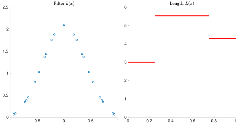
Figure 1: On the left, the conditions on the filter $k(x)$. On the right, the step-function $L(x)$.

Since all the points where $k$ is evaluated are distinct, we can find an even, non-negative, bounded and continuous measurable function $k$ supported on $(-1,1)$, that respects all conditions. The most simple example is a piecewise linear function connecting all the conditions shown in Figure 1. In this case, $\|k\|_{1}>1$, but notice that the filter $k^{\prime}(x):=k(x)/\|k\|_{1}$ and the same length function $L(x)$ produce the matrix $K^{\prime}_{n}=K_{n}/\|k\|_{1}$, that is still a counterexample to Conjecture 2’, since it has a negative eigenvalue, and $0\leq\kappa^{\prime}(x,\theta)=\kappa(x,\theta)/\|k\|_{1}\leq 2/\|k\|_{1}<2$.

6 Conclusions

In this work we tackle the open problems and conjectures left unsolved in [11], which regard the convergence of the ALIF method.

In particular, we first review basic and fundamental properties of sequences of matrices, with particular emphasis on the GLT sequences, approximating classes of sequences of matrices and their spectral properties. Then we recall the ALIF method, its known properties and the two conjectures proposed in [11]. In Theorem 4.1 we prove that Conjecture 1 actually holds true. To achieve this result, we rely on several new technical lemmata on approximating classes of sequences convergence of certain matrix sequences, namely the Almost-Hermitian Sequences and Almost-Hermitian GLT Sequences, and some new results on spectral symbols. On the other hand, we show by counterexample that Conjecture 2 cannot hold as it is. In particular we are able to show that the current formulation of the conjecture is too loose. We propose, then, a tighter formulation as Conjecture 2’. However, even in this case we are able to find a counterexample to the statement.

It remains an open problem if the ALIF algorithm can be proved to be convergent at all. We plan to study this problem in a future work.

Appendix A Appendix: Technical results

In this appendix, we provide the full details on some technical steps that are necessary for our analysis. For convenience, we have split the appendix into various subsections, according to the specific nature of the results contained therein. Note that in the following, if $A$ is any subset of $[0,1]$, then $A^{C}$ is its complement set in $[0,1]$.

A.1 Auxiliary Result

Lemma 2

Let $a:[0,1]\to\mathbb{C}$ be a bounded function and call $\alpha$-oscillation of $a$ the function

$$\omega_{\alpha}(x):=\sup_{z\in B_{\alpha}(x)\cap[0,1]}|a(z)|-\inf_{z\in B_{\alpha}(x)\cap[0,1]}|a(z)|,$$

where $B_{\alpha}(x)$ is the open ball with centre $x$ and radius $\alpha$. If $a$ is continuous a.e., then also $\omega_{\alpha}$ is continuous a.e.

Proof. Let $E$ be the set of discontinuity points for $a$, and define

$$Z:=\set{x\in[0,1]}{x-\alpha\in E\text{ or }x+\alpha\in E}.$$

Note that the measure of $Z$ is at most two times the measure of $E$, so it is zero. Let now $x\in Z^{C}$ and $a(x)=b$. We know that both $x-\alpha$ and $x+\alpha$ (when they are inside $[0,1]$) are continuity points for $a$, so given any $\varepsilon>0$, there exists $\delta>0$ such that

$$|a(x-\alpha)-a(x-\alpha+y)|\leq\varepsilon,\quad|a(x+\alpha)-a(x+\alpha+y)|\leq\varepsilon\qquad\forall|y|<\delta.$$

As a consequence, for every $0<y<\delta$ the following holds

$$\sup_{z\in B_{\alpha}(x+y)\cap[0,1]}|a(z)| =\max\left\{\sup_{z\in(x+y-\alpha,x+\alpha)\cap[0,1]}|a(z)|,\sup_{z\in[x+\alpha,x+\alpha+y)\cap[0,1]}|a(z)|\right\}$$

$$\implies\sup_{z\in B_{\alpha}(x+y)\cap[0,1]}|a(z)| \leq\max\left\{\sup_{z\in B_{\alpha}(x)\cap[0,1]}|a(z)|,|a(x+\alpha)|+\varepsilon\right\}\leq\sup_{z\in B_{\alpha}(x)\cap[0,1]}|a(z)|+\varepsilon,$$

$$\sup_{z\in B_{\alpha}(x+y)\cap[0,1]}|a(z)| \geq\sup_{z\in(x+y-\alpha,x+\alpha)\cap[0,1]}|a(z)|\geq\sup_{z\in B_{\alpha}(x)\cap[0,1]}|a(z)|-\varepsilon,$$

$$\inf_{z\in B_{\alpha}(x+y)\cap[0,1]}|a(z)| =\min\left\{\inf_{z\in(x+y-\alpha,x+\alpha)\cap[0,1]}|a(z)|,\inf_{z\in[x+\alpha,x+\alpha+y)\cap[0,1]}|a(z)|\right\}$$

$$\implies\inf_{z\in B_{\alpha}(x+y)\cap[0,1]}|a(z)| \geq\min\left\{\inf_{z\in B_{\alpha}(x)\cap[0,1]}|a(z)|,|a(x+\alpha)|-\varepsilon\right\}\geq\inf_{z\in B_{\alpha}(x)\cap[0,1]}|a(z)|-\varepsilon,$$

$$\inf_{z\in B_{\alpha}(x+y)\cap[0,1]}|a(z)| \leq\inf_{z\in(x+y-\alpha,x+\alpha)\cap[0,1]}|a(z)|\leq\inf_{z\in B_{\alpha}(x)\cap[0,1]}|a(z)|+\varepsilon.$$

$$\left|\sup_{z\in B_{\alpha}(x+y)\cap[0,1]}|a(z)|-\sup_{z\in B_{\alpha}(x)\cap[0,1]}|a(z)|\right|\leq\varepsilon,\qquad\left|\inf_{z\in B_{\alpha}(x+y)\cap[0,1]}|a(z)|-\inf_{z\in B_{\alpha}(x)\cap[0,1]}|a(z)|\right|\leq\varepsilon.$$ (11)

With an analogous argument we can show that (11) holds also for $-\delta<y<0$ and even if $x+\alpha$ or $x-\alpha$ are not inside $[0,1]$, so

$$|\omega_{\alpha}(x)-\omega_{\alpha}(x+y)|\leq\left|\sup_{z\in B_{\alpha}(x)\cap[0,1]}|a(z)|-\sup_{z\in B_{\alpha}(x+y)\cap[0,1]}|a(z)|\right|+\left|\inf_{z\in B_{\alpha}(x+y)\cap[0,1]}|a(z)|-\inf_{z\in B_{\alpha}(x)\cap[0,1]}|a(z)|\right|\leq 2\varepsilon.$$

This is enough to prove that $\omega_{\alpha}$ is continuous at every point of $Z^{C}$, meaning it is continuous a.e.      

Lemma 3

Let $x_{i}=\frac{i}{n-1}$ and

$$D^{\prime}_{n}(a):=\operatorname{diag}([a(x_{i})]_{i=0,\dots,n-1})$$

for any Riemann-Integrable function $a:[0,1]\to\mathbb{C}$. Then

$$\{D^{\prime}_{n}(a)\}_{n}\sim_{GLT}a(x).$$

Proof. First of all, let us prove it in the case $a(x)$ continuous. Notice that

$$\left|\left[D^{\prime}_{n}(a)-D_{n}(a)\right]_{i,i}\right|=|a(x_{i-1})-a(i/n)|\leq\omega_{a}\left(\left|\frac{i-1}{n-1}-\frac{i}{n}\right|\right)=\omega_{a}\left(\left|\frac{n-i}{n(n-1)}\right|\right)\leq\omega_{a}(1/n)$$

where $\omega_{a}$ is the continuity modulus of $a(x)$. Since $\omega_{a}(x)\xrightarrow{x\to 0}0$, we obtain that $\|D^{\prime}_{n}(a)-D_{n}(a)\|\xrightarrow{n\to\infty}0$ and in particular, from Proposition 1, we know that $\{D_{n}(a)-D_{n}^{\prime}(a)\}_{n}$ is zero-distributed. The thesis follows from GLT 3 and GLT 4.

Suppose now that $a(x)$ is Riemann-Integrable. From the density of the continuous function in $L^{1}([0,1])$, we know that there exists a sequence of continuous functions $a_{m}(x)$ converging in $L^{1}([0,1])$ to $a(x)$. Notice that $a-a_{m}$ is Riemann-Integrable for any $m$.

$$\lim_{m\to\infty}\limsup_{n\to\infty}\frac{1}{n}\|D_{n}^{\prime}(a_{m})-D^{\prime}_{n}(a)\|_{1} =\lim_{m\to\infty}\limsup_{n\to\infty}\frac{1}{n}\sum_{i=0}^{n-1}\left|a_{m}(x_{i})-a(x_{i})\right|$$

$$=\lim_{m\to\infty}\int_{0}^{1}|a_{m}(x)-a(x)|\,{{\rm d}}x=0,$$

and Theorem 2.1 shows that

$$\{D_{n}^{\prime}(a_{m})\}_{n}\xrightarrow{a.c.s.}\{D_{n}^{\prime}(a)\}_{n}.$$

The thesis follows from GLT 5.      

A.2 Almost-Hermitian Sequences

From now on, we say that a sequence $\{A_{n}\}_{n}$ is almost-Hermitian if there exists an Hermitian sequence $\{\widetilde{A}_{n}\}_{n}$ such that $\|A_{n}-\widetilde{A}_{n}\|_{2}=o(\sqrt{n})$.

Lemma 4

Suppose $\{A_{n}\}_{n}\sim_{GLT}k$ is an almost-Hermitian sequence. In this case, $k$ is real valued and

$$\{A_{n}\}_{n}\sim_{GLT,\sigma,\lambda}k.$$

Proof. Since $A_{n}=\widetilde{A}_{n}+(A_{n}-\widetilde{A}_{n})$ where $\widetilde{A}_{n}$ is Hermitian and $\|A_{n}-\widetilde{A}_{n}\|_{2}=o(\sqrt{n})$, from GLT 2 we conclude that $\{A_{n}\}_{n}\sim_{\lambda}k$.      

Lemma 5

The set of almost-Hermitian sequences is a real vectorial space.

Proof. If $\{A_{n}\}_{n}$ is an almost-Hermitian sequence and $c\in\mathbb{R}$, then

$$\|cA_{n}-c\widetilde{A}_{n}\|_{2}=|c|\|A_{n}-\widetilde{A}_{n}\|_{2}=o(\sqrt{n}).$$

If $\{B_{n}\}_{n}$ is also almost-Hermitian, then

$$\|A_{n}+B_{n}-\widetilde{A}_{n}-\widetilde{B}_{n}\|_{2}\leq\|A_{n}-\widetilde{A}_{n}\|_{2}+\|B_{n}-\widetilde{B}_{n}\|_{2}=o(\sqrt{n}).$$

     

Lemma 6

Given a sequence of almost-Hermitian sequences $\{B_{n,m}\}_{n}$ suppose that there exists a sequence $\{B_{n}\}_{n}$ with

$$\lim_{m\to\infty}\limsup_{n\to\infty}\frac{1}{n}\|B_{n,m}-B_{n}\|_{2}^{2}=0.$$

In this case, $\{B_{n}\}_{n}$ is almost-Hermitian.

Proof. From the definition of almost-Hermitian sequences, we can find $\widetilde{B}_{n,m}$ Hermitian matrices with $\|B_{n,m}-\widetilde{B}_{n,m}\|_{2}=o(\sqrt{n})$. Let us now estimate the norm of the imaginary part of $\{B_{n}\}_{n}$.

$$\|\Im(B_{n})\|_{2} =\frac{1}{2}\|B_{n}-B_{n}^{*}\|_{2}$$

$$\leq\frac{1}{2}\left(\|B_{n}-B_{n,m}\|_{2}+\|B_{n,m}-\widetilde{B}_{n,m}\|_{2}+\|\widetilde{B}_{n,m}-B_{n,m}^{*}\|_{2}+\|B_{n,m}^{*}-B_{n}^{*}\|_{2}\right)$$

$$=\|B_{n}-B_{n,m}\|_{2}+\|B_{n,m}-\widetilde{B}_{n,m}\|_{2}$$

$$\implies\limsup_{n\to\infty}\frac{1}{\sqrt{n}}\|\Im(B_{n})\|_{2} =\lim_{m\to\infty}\limsup_{n\to\infty}\frac{1}{\sqrt{n}}\|\Im(B_{n})\|_{2}$$

$$\leq\lim_{m\to\infty}\limsup_{n\to\infty}\frac{1}{\sqrt{n}}\|B_{n}-B_{n,m}\|_{2}+\frac{1}{\sqrt{n}}\|B_{n,m}-\widetilde{B}_{n,m}\|_{2}=0$$

$$\implies\|\Im(B_{n})\|_{2} =o(\sqrt{n}).$$

Since $B_{n}=\Re(B_{n})+\textnormal{i}\Im(B_{n})$, the sequence $\{B_{n}\}_{n}$ is an Hermitian sequence $\{\Re(B_{n})\}_{n}$ plus a $o(\sqrt{n})$ correction, thus it is an almost-Hermitian sequence.      

A.3 Almost-Hermitian GLT Sequences

The following result is formulated so that it can be applied to the problem at hand, but the same argument works also with $D_{n}(f_{p})$ instead of $D_{n}^{\prime}(f_{p})$.

Theorem A.1

Given any Riemann Integrable function $a:[0,1]\to\mathbb{C}$ and any natural number $m$, denote

$$A_{n}(a,m):=D_{n}^{\prime}(a)T_{n}(e^{\textnormal{i}m\theta})+D_{n}^{\prime}(a)^{*}T_{n}(e^{\textnormal{i}m\theta})^{*},$$

where

$$D^{\prime}_{n}(a):=\operatorname{diag}([a(x_{i})]_{i=0,\dots,n-1})$$

and $x_{i}=\frac{i}{n-1}$. In this case, if $a_{0},a_{1},\dots,a_{p-1}$ are Riemann Integrable functions, then

$$\left\{\frac{1}{2}A_{n}(a_{0},0)+\sum_{m=1}^{p-1}A_{n}(a_{m},m)\right\}_{n}$$

is an almost-Hermitian sequence for every positive number $p$.

Proof. First of all, from GLT 3,4 and Lemma 3, we know that

$$\{A_{n}(a,m)\}_{n}\sim_{GLT}2\Re(a(x)e^{\textnormal{i}m\theta}).$$

If $m=0$, then $A_{n}(a,m)$ is Hermitian for every $n$, so the thesis follows. Suppose now that $m>0$ and define the Hermitian matrix $\widetilde{A}_{n}(a,m)$ as

$$[\widetilde{A}_{n}(a,m)]_{i,j}=\begin{cases}a(x_{j-1}),&i-j=m,\\ \overline{a}(x_{i-1}),&i-j=-m,\\ 0,&\text{otherwise.}\end{cases}$$

Let $Z_{n}=A_{n}(a,m)-\widetilde{A}_{n}(a,m)$, and notice that

$$[Z_{n}]_{i,j}=\begin{cases}a(x_{i-1})-a(x_{j-1}),&i-j=m,\\ 0,&\text{otherwise.}\end{cases}$$

Notice that if $\omega_{\alpha}$ is the $\alpha$-oscillation relative to $a$, defined as

$$\omega_{\alpha}(x):=\sup_{z\in B_{\alpha}(x)\cap[0,1]}|a(z)|-\inf_{z\in B_{\alpha}(x)\cap[0,1]}|a(z)|,$$

then $\omega_{\alpha}\xrightarrow{\alpha\to 0}0$ a.e. since

$$a\text{ continuous on }x\implies\omega_{\alpha}(x)\xrightarrow{\alpha\to 0}0.$$

We can thus fix $\varepsilon>0$ and find $\alpha_{\varepsilon}$ (that we call $\alpha$ for simplicity) such that

$$E:=\set{x\in[0,1]:\omega_{\alpha}(x)\geq\varepsilon},\quad\mu(E)<\varepsilon/2.$$

Notice that $a$ is bounded and continuous a.e., so by Lemma 2, $\omega_{\alpha}$ is also continuous a.e. and thus $E^{C}$ is an open set up to a negligible set. Every open set can be approximated from the inside by a finite union of open intervals, so we can take $G\subseteq E^{C}$ a finite union of open intervals with measure $\mu(G)>\mu(E^{C})-\varepsilon/2>1-\varepsilon$. We can approximate the measure of $G$ as

$$\lim_{n\to\infty}\frac{1}{n}\#\set{i}{0\leq i\leq n-1,x_{i}\in G}=\mu(G)>1-\varepsilon.$$

Let $N$ be an index such that $m/N<\alpha$ and

$$\frac{1}{n}\#\set{i}{0\leq i\leq n-1,x_{i}\in G}>1-2\varepsilon\quad\forall n>N.$$

If $\|a\|_{\infty}=M$ and $n>N$, we have

$$\|Z_{n}\|_{2}^{2} =\sum_{j=1}^{n-m}|a(x_{j+m-1})-a(x_{j-1})|^{2}$$

$$=\sum_{j\leq n-m}^{x_{j-1}\not\in G}|a(x_{j+m-1})-a(x_{j-1})|^{2}+\sum_{j\leq n-m}^{x_{j-1}\in G}|a(x_{j+m-1})-a(x_{j-1})|^{2}$$

$$\leq\#\set{i}{0\leq i\leq n-1,x_{i}\in G^{C}}\cdot 4M^{2}+\sum_{j\leq n-m}^{x_{j-1}\in E^{C}}\omega_{\alpha}(x_{j-1})^{2}$$

$$\leq 8\varepsilon nM^{2}+n\varepsilon^{2}.$$

As a consequence

$$\limsup_{n\to\infty}\frac{1}{n}\|Z_{n}\|_{2}^{2}\leq 8\varepsilon M^{2}+\varepsilon^{2}$$

for every $\varepsilon>0$, so

$$\limsup_{n\to\infty}\frac{1}{n}\|Z_{n}\|_{2}^{2}=0.$$

We have thus shown that $\{A_{n}(a,m)\}_{n}$ is almost-Hermitian, and Lemma 5 let us conclude that

$$\left\{\frac{1}{2}A_{n}(a_{0},0)+\sum_{m=1}^{p-1}A_{n}(a_{m},m)\right\}_{n}$$

is also an almost-Hermitian sequence for every positive number $p$.

References

- [1] X. An. Local rub-impact fault diagnosis of a rotor system based on adaptive local iterative filtering. Transactions of the Institute of Measurement and Control, 39(5):748–753, 2017.
- [2] X. An, C. Li, and F. Zhang. Application of adaptive local iterative filtering and approximate entropy to vibration signal denoising of hydropower unit. Journal of Vibroengineering, 18(7):4299–4311, 2016.
- [3] X. An and L. Pan. Wind turbine bearing fault diagnosis based on adaptive local iterative filtering and approximate entropy. Proceedings of the Institution of Mechanical Engineers, Part C: Journal of Mechanical Engineering Science, 231(17):3228–3237, 2017.
- [4] X. An, W. Yang, and X. An. Vibration signal analysis of a hydropower unit based on adaptive local iterative filtering. Proceedings of the Institution of Mechanical Engineers, Part C: Journal of Mechanical Engineering Science, 231(7):1339–1353, 2017.
- [5] X. An, H. Zeng, and C. Li. Demodulation analysis based on adaptive local iterative filtering for bearing fault diagnosis. Measurement, 94:554–560, 2016.
- [6] G. Barbarino and S. Serra-Capizzano. Non-hermitian perturbations of hermitian matrix-sequences and applications to the spectral analysis of the numerical approximation of partial differential equations. Numerical Linear Algebra with Applications, 27(3):e2286, 2020.
- [7] A. Cicone. Nonstationary signal decomposition for dummies. In Advances in Mathematical Methods and High Performance Computing, pages 69–82. Springer, 2019.
- [8] A. Cicone. Iterative filtering as a direct method for the decomposition of nonstationary signals. Numerical Algorithms, pages 1–17, 2020.
- [9] A. Cicone. Multivariate fast iterative filtering for the decomposition of nonstationary signals. submitted, 2020.
- [10] A. Cicone and P. Dell’Acqua. Study of boundary conditions in the iterative filtering method for the decomposition of nonstationary signals. Journal of Computational and Applied Mathematics, 373:112248, 2020.
- [11] A. Cicone, C. Garoni, and S. Serra-Capizzano. Spectral and convergence analysis of the discrete alif method. Linear Algebra and its Applications, 580:62–95, 2019.
- [12] A. Cicone, J. Liu, and H. Zhou. Adaptive local iterative filtering for signal decomposition and instantaneous frequency analysis. Applied and Computational Harmonic Analysis, 41(2):384–411, 2016.
- [13] A. Cicone, J. Liu, and H. Zhou. Hyperspectral chemical plume detection algorithms based on multidimensional iterative filtering decomposition. Phil. Trans. R. Soc. A: Math. Phys. Eng. Sci., 374(2065):2015.0196, 2016.
- [14] A. Cicone and H.-T. Wu. How Nonlinear-Type Time-Frequency Analysis Can Help in Sensing Instantaneous Heart Rate and Instantaneous Respiratory Rate from Photoplethysmography in a Reliable Way. Front. Physiol., 8: 701, 2017.
- [15] A. Cicone and H.-T. Wu. Convergence analysis of adaptive locally iterative filtering and sift method. submitted, 2020.
- [16] A. Cicone and H. Zhou. Multidimensional iterative filtering method for the decomposition of high-dimensional non-stationary signals. Numer. Math. Theory Methods Appl., 10(2):278–298, 2017.
- [17] A. Cicone and H. Zhou. Numerical analysis for iterative filtering with new efficient implementations based on fft. submitted, 2020.
- [18] A. Cicone and H. Zhou. One or two frequencies? the iterative filtering answers. preprint, 2020.
- [19] K. Dragomiretskiy and D. Zosso. Variational mode decomposition. IEEE transactions on signal processing, 62(3):531–544, 2013.
- [20] C. Garoni and S. Serra-Capizzano. The theory of Generalized Locally Toeplitz sequences: theory and applications, volume I. Springer, 2017.
- [21] H. Ghobadi, C. Savas, L. Spogli, F. Dovis, A. Cicone, M. Cafaro. A Comparative Study of Different Phase Detrending Algorithms for Scintillation Monitoring. submitted, (2020).
- [22] H. Ghobadi, L. Spogli, L. Alfonsi, C. Cesaroni, A. Cicone, N. Linty, V. Romano, and M. Cafaro. Disentangling ionospheric refraction and diffraction effects in gnss raw phase through fast iterative filtering technique. GPS Solutions, 24(3):1–13, 2020.
- [23] J. Gilles. Empirical wavelet transform. IEEE transactions on signal processing, 61(16):3999–4010, 2013.
- [24] T. Y. Hou and Z. Shi. Adaptive data analysis via sparse time-frequency representation. Advances in Adaptive Data Analysis, 3(01n02):1–28, 2011.
- [25] T. Y. Hou, M. P. Yan, and Z. Wu. A variant of the emd method for multi-scale data. Advances in Adaptive Data Analysis, 1(04):483–516, 2009.
- [26] C. Huang, L. Yang, and Y. Wang. Convergence of a convolution-filtering-based algorithm for empirical mode decomposition. Advances in Adaptive Data Analysis, 1(04):561–571, 2009.
- [27] N. E. Huang, Z. Shen, S. R. Long, M. C. Wu, H. H. Shih, Q. Zheng, N.-C. Yen, C. C. Tung, and H. H. Liu. The empirical mode decomposition and the hilbert spectrum for nonlinear and non-stationary time series analysis. Proceedings of the Royal Society of London. Series A: mathematical, physical and engineering sciences, 454(1971):903–995, 1998.
- [28] S. J. Kim and H. Zhou. A multiscale computation for highly oscillatory dynamical systems using empirical mode decomposition (emd)–type methods. Multiscale Modeling & Simulation, 14(1):534–557, 2016.
- [29] Y. Li, X. Wang, Z. Liu, X. Liang, and S. Si. The entropy algorithm and its variants in the fault diagnosis of rotating machinery: A review. IEEE Access, 6:66723–66741, 2018.
- [30] L. Lin, Y. Wang, and H. Zhou. Iterative filtering as an alternative algorithm for empirical mode decomposition. Advances in Adaptive Data Analysis, 1(04):543–560, 2009.
- [31] M. Materassi, M. Piersanti, G. Consolini, P. Diego, G. D’Angelo, I. Bertello, and A. Cicone. Stepping into the equatorward boundary of the auroral oval: preliminary results of multi scale statistical analysis. Annals of Geophysics, 62(4):455, 2019.
- [32] S. Meignen and V. Perrier. A new formulation for empirical mode decomposition based on constrained optimization. IEEE Signal Processing Letters, 14(12):932–935, 2007.
- [33] I. Mitiche, G. Morison, A. Nesbitt, M. Hughes-Narborough, B. G. Stewart, and P. Boreham. Classification of partial discharge signals by combining adaptive local iterative filtering and entropy features. Sensors, 18(2):406, 2018.
- [34] E. Papini, A. Cicone, M. Piersanti, L. Franci, P. Hellinger, S. Landi, and A. Verdini. Multidimensional iterative filtering: a new approach for investigating plasma turbulence in numerical simulations. Journal of Plasma Physics, 2020.
- [35] G. Piersanti, M. Piersanti, A. Cicone, P. Canofari, and M. Di Domizio. An inquiry into the structure and dynamics of crude oil price using the fast iterative filtering algorithm. Energy Economics, 2020.
- [36] M. Piersanti, M. Materassi, A. Cicone, L. Spogli, H. Zhou, and R. G. Ezquer. Adaptive local iterative filtering: A promising technique for the analysis of nonstationary signals. Journal of Geophysical Research: Space Physics, 123(1):1031–1046, 2018.
- [37] N. Pustelnik, P. Borgnat, and P. Flandrin. A multicomponent proximal algorithm for empirical mode decomposition. In 2012 Proceedings of the 20th European Signal Processing Conference (EUSIPCO), pages 1880–1884. IEEE, 2012.
- [38] I. W. Selesnick. Resonance-based signal decomposition: A new sparsity-enabled signal analysis method. Signal Processing, 91(12):2793–2809, 2011.
- [39] S. Sfarra, A. Cicone, B. Yousefi, C. Ibarra-Castanedo, S. Perilli, and X. Maldague. Improving the detection of thermal bridges in buildings via on-site infrared thermography: The potentialities of innovative mathematical tools. Energy and Buildings, 182:159–171, 2019.
- [40] R. Sharma, R. B. Pachori, and A. Upadhyay. Automatic sleep stages classification based on iterative filtering of electroencephalogram signals. Neural Computing and Applications, 28(10):2959–2978, 2017.
- [41] L. Spogli, M. Piersanti, C. Cesaroni, M. Materassi, A. Cicone, L. Alfonsi, V. Romano, and R. G. Ezquer. Role of the external drivers in the occurrence of low-latitude ionospheric scintillation revealed by multi-scale analysis. Journal of Space Weather and Space Climate, 9:A35, 2019.
- [42] L. Spogli, M. Piersanti, C. Cesaroni, M. Materassi, A. Cicone, L. Alfonsi, V. Romano, and R. G. Ezquer. Role of the external drivers in the occurrence of low-latitude ionospheric scintillation revealed by multi-scale analysis. In 2019 URSI Asia-Pacific Radio Science Conference (AP-RASC), number 8738254, pages 1–1, 2019.
- [43] A. Stallone, A. Cicone, and M. Materassi. New insights and best practices for the successful use of Empirical Mode Decomposition, Iterative Filtering and derived algorithms. Scientific Reports, 2020.
- [44] M. E. Torres, M. A. Colominas, G. Schlotthauer, and P. Flandrin. A complete ensemble empirical mode decomposition with adaptive noise. In 2011 IEEE international conference on acoustics, speech and signal processing (ICASSP), pages 4144–4147. IEEE, 2011.
- [45] N. Ur Rehman and D. P. Mandic. Filter bank property of multivariate empirical mode decomposition. IEEE transactions on signal processing, 59(5):2421–2426, 2011.
- [46] Z. Wu and N. E. Huang. Ensemble empirical mode decomposition: a noise-assisted data analysis method. Advances in adaptive data analysis, 1(01):1–41, 2009.
- [47] D. Yang, B. Wang, G. Cai, and J. Wen. Oscillation mode analysis for power grids using adaptive local iterative filter decomposition. International Journal of Electrical Power & Energy Systems, 92:25–33, 2017.
- [48] J.-R. Yeh, J.-S. Shieh, and N. E. Huang. Complementary ensemble empirical mode decomposition: A novel noise enhanced data analysis method. Advances in adaptive data analysis, 2(02):135–156, 2010.
- [49] S. Yu, J. Ma, and S. Osher. Geometric mode decomposition. Inverse Problems & Imaging, 12(4):831–852, 2018.
- [50] Z.-G. Yu, V. Anh, Y. Wang, D. Mao, and J. Wanliss. Modeling and simulation of the horizontal component of the geomagnetic field by fractional stochastic differential equations in conjunction with empirical mode decomposition. Journal of Geophysical Research: Space Physics, 115(A10), 2010.
- [51] J. Zheng, J. Cheng, and Y. Yang. Partly ensemble empirical mode decomposition: An improved noise-assisted method for eliminating mode mixing. Signal Processing, 96:362–374, 2014.