Linear-Quadratic Zero-Sum Mean-Field Type Games:
Optimality Conditions and Policy Optimization

Abstract.

In this paper, zero-sum mean-field type games (ZSMFTG) with linear dynamics and quadratic cost are studied under infinite-horizon discounted utility function. ZSMFTG are a class of games in which two decision makers whose utilities sum to zero, compete to influence a large population of indistinguishable agents. In particular, the case in which the transition and utility functions depend on the state, the action of the controllers, and the mean of the state and the actions, is investigated. The optimality conditions of the game are analysed for both open-loop and closed-loop controls, and explicit expressions for the Nash equilibrium strategies are derived. Moreover, two policy optimization methods that rely on policy gradient are proposed for both model-based and sample-based frameworks. In the model-based case, the gradients are computed exactly using the model, whereas they are estimated using Monte-Carlo simulations in the sample-based case. Numerical experiments are conducted to show the convergence of the utility function as well as the two players’ controls.

1. Introduction

Decision making in multi-agent systems has recently received an increasing interest from both theoretical and empirical viewpoints. For instance, multi-agent reinforcement learning (MARL) has been applied successfully to problems ranging from self-driving cars and robotics to games, while game-theoretic models have been exploited to study several prominent decision-making problems in engineering, economics and finance.

In multi-agent systems, a large number of interacting agents either cooperate or compete to optimize a certain individual or common goal. MARL and stochastic games were shown to model well systems with a small number of agents. However, as the number of agents becomes large, analysing such systems becomes intractable due to the exponential growth of agent interactions and the prohibitive computational cost. To tackle this issue, mean-field approximations, borrowed from statistical physics, were considered to study the limit behaviour of systems in which the agents are indistinguishable and their decisions are influenced by the empirical distribution of the other agents.

Mean-field games (MFGs) [42, 39] and their variants mean-field type control (MFC) [14] and mean-field type games (MFTG) [10] consist of studying the global behaviour of systems composed of infinitely many agents which interact in a symmetric manner. In particular, the mean-field approximation captures all agent-to-agent interactions that, individually, have a negligible influence on the overall system’s evolution.

An MFG corresponds to the asymptotic limit of the situation in which all the agents compete to minimize their individual utility. In this case, the solution concept is a Nash equilibrium, in which a typical agent is worse-off if she deviates unilaterally. From the point of view of the global system, a better solution can be found by a central planner who tries to minimize the social utility by prescribing the control that each agent should use. This leads to the notion of MFC, which can be viewed as the optimal control of a McKean-Vlasov (MKV) dynamics, in which the evolution of the state process is influenced by its own distribution. Last, mean-field type games are a framework that models control problems involving several decision makers and mean-field interactions. Typical motivations are problems in which large coalitions compete or in which several agents try to influence a large population [32, 16]. These three types of models have found numerous applications [12], e.g. in finance [21], energy production [13, 8], crowd motion [3, 4], wireless communications [47, 40, 45], distributed robotics [43] and systemic risk [24, 34].

In the past decade, many contributions have contributed to develop the theory of such mean-field problems. In order to study their solutions, a key point is the derivation of optimality conditions, which are typically phrased either in terms of partial differential equations (PDEs) or in terms of forward-backward stochastic differential equations (FBSDEs). For a detailed account, see e.g. [20, 15, 23] and the references therein. As a cornerstone for applications, the development of numerical methods for these mean-field problems has also attracted a growing interest. Assuming full knowledge of the model, methods for which convergence guarantees have been established include finite difference schemes for partial differential equations [2, 1], semi-Lagrangian schemes [22], augmented Lagrangian or primal-dual methods [5, 18, 17], value iteration algorithm [9], or neural network based stochastic methods [26, 27]; see e.g. [6] for a recent overview. However, in many practical situations, the model is not fully known and these methods can not be employed. Hence model-free or sample-based methods, in which the optimization is performed while having only access to a simulator instead of knowing the model, have recently been investigated. For mean-field games, fixed-point [38] or fictitious play scheme  [35] have been combined with model-free methods to compute the best response, whereas for mean-field control problems, the solution has been approximated using policy gradient [28] or Q-learning [29, 37]. Despite recent progress, these methods remain restricted to mean-field problems with simple structures which have a common point: the decision makers are either infinitesimal and identical players or a single central planner. More complex models are often needed to tackle applications, such as settings in which a mean-field dynamics is influenced by several distinguishable decision makers. Such situations can typically be modeled by a MFTG.

An archetypal MFTG is the case of mean-field zero-sum games. Two-player zero-sum games in their standard stochastic form, with no mean-field interactions, have been extensively studied in the literature [49]. In this class of games, two decision makers compete to respectively maximize and minimize the same utility function. The large literature on this topic is motivated by many applications and by connections with robust control [11]. Recently, generalizations to the case where the state dynamics is of MKV type have been introduced in continuous time over a finite time horizon. Optimality conditions have been derived using the theory of backward stochastic differential equations (BSDEs) in [50], using the dynamic programming principle and partial differential equations (PDEs) in [30] or using a weak formulation in [31]. All these works assume that the controls take values in a compact space, and hence are not applicable to a general linear-quadratic setting. Along a different line, zero-sum games with mean-field interactions have also attracted interest for their connections with generative adversarial nets (GANs) [33, 19].

Although general stochastic problems with mean-field interactions can be studied from a theoretical perspective, explicit computation of the solution and numerical illustration of the Nash equilibrium are challenging. In standard optimal control, linear-quadratic (LQ) models, where the dynamics are linear and the cost is quadratic, usually have analytical or easily tractable solutions, which makes them very popular. These problems have also been considered in the optimization and machine learning communities, since algorithms with proof of convergence can be developed, see e.g. [36] where the authors prove convergence of model-based and sample-based policy gradient methods for a LQ optimal control problem. Sample-based methods have also been used to solve (standard) LQ zero-sum games. In [7], a discrete-time linear quadratic zero-sum game with infinite time horizon is studied and a Q-learning algorithm is proposed, which is proved to converge to the Nash equilibrium. In [51], the authors study LQ zero-sum games and propose three projected nested-gradient methods that are shown to converge to the Nash equilibrium of the game. However, none of these contributions tackle mean-field interactions in a zero-sum setting.

In the present work, under a discrete time, infinite-horizon and discounted utility function, we investigate zero-sum mean-field type games (ZSMFTG) of linear-quadratic type, which, to the best of our knowledge, had not been the focus of any work before. In particular, we address the case in which the transition and utility functions do not only depend on the state and the action of the controllers, but also the mean of the state and the actions. Moreover, the state is subject to a common noise. The structure of the problem and the infinite horizon regime allow us to identify the form of the equilibrium controls as linear combinations of the state and its mean conditioned on the common noise, both in the open-loop and the closed-loop settings. To learn the equilibrium, we extend the policy-gradient techniques developed in [28] for MFC, to the ZSMFTG framework. We design policy optimization methods in which the gradients are either computed exactly using the LQ model or estimated using Monte-Carlo samples when the model is not fully known.

The rest of the paper is organized as follows. In Section 2, the zero-sum mean-field type game is formulated, preceded by a $N$-agent control problem which motivates this setting. In Section 3, we present the rigorous probabilistic setup for the zero-sum mean-field type game under consideration. Open-loop controls are investigated in Section 4. After defining the set of admissible controls, we prove a Pontryagin maximum principle giving necessary and sufficient conditions of optimality, see Propositions 12 and 14. Section 5 considers closed-loop controls which are linear in the state and the mean. Focusing on the coefficients of the linear combination, we define a notion of admissible controls and prove sufficient conditions of optimality, see Proposition 36 and Corollary 39. The connection between equilibria in the open-loop and the closed-loop information structures are studied in Section 6, see Lemma 42 and Remark 43. Focusing on closed-loop controls, expressions for the gradient of the utility function and a necessary condition of optimality are derived in Section 7, and both model-based and model-free policy optimization methods are proposed. In Subsection 7.4, we report numerical experiments to show the convergence of the controls and the utility function. Section 8 concludes the paper.

2. Model and Problem Formulation

In this section, we first present a zero-sum game in which two controllers compete to influence a population of agents. The agents interact in a symmetric way, through the empirical distribution of their states and actions. We then present a mean-field version of the game (corresponding to the situation where $N\to+\infty$), in which the two controllers influence a state whose dynamics is of MKV type.

2.1. $N$-agent problem

Consider a system composed of a population $\{1,\dots,N\}$ with $N$ indistinguishable agents. We investigate the case in which these agents have symmetric interactions and are influenced by two decision makers, also called controllers or players, competing to optimize a criterion. In particular, we are interested in the linear-quadratic zero-sum case. Here, the state evolution of an agent $i\in\{1,\dots,N\}$ is given by

(1) $$x^{i}_{t+1}=Ax^{i}_{t}+\bar{A}\bar{x}_{t}+B_{1}u^{i}_{1,t}+\bar{B}_{1}\bar{u}_{1,t}+B_{2}u^{i}_{2,t}+\bar{B}_{2}\bar{u}_{2,t}+\epsilon^{i}_{t+1}+\epsilon^{0}_{t+1},$$

with initial condition $x^{i}_{0}=\epsilon^{i}_{0}+\epsilon^{0}_{0}$, where $x^{i}_{0}$ is the initial state of agent $i$ to which we introduce randomness with $\epsilon^{i}_{0}$ and $\epsilon^{0}_{0}$. At each time $t$, $x_{t}^{i}\in\mathbb{R}^{d}$ corresponds to the state of the $i$-th agent in the population, and $u^{i}_{1,t}\in\mathbb{R}^{\ell}$ and $u^{i}_{2,t}\in\mathbb{R}^{\ell}$ are the controls prescribed to this agent respectively by the first and the second decision maker. The noise terms $\epsilon^{0}_{t+1}$ and $\epsilon^{i}_{t+1}$ are independent of each other and of $\epsilon^{0}_{0}$ and $\epsilon^{i}_{0}$. Moreover, the noise terms $\epsilon^{0}_{t+1}$ for $t\geq 0$ are assumed to be identically distributed with mean $0$, and similarly for $\epsilon^{i}_{t+1}$ for $t\geq 0$. The interpretation of the noise terms is that $\epsilon^{0}_{t}$ is a common noise affecting the position of all the agents, whereas $\epsilon^{i}_{t}$ is an indiosyncratic noise affecting only the position of the $i$-th agent. $A,\bar{A},B_{i},\bar{B}_{i}$ are fixed matrices with suitable dimensions. Here, $\bar{x}_{t}=\frac{1}{N}\sum_{i=1}^{N}x_{t}^{i}$, is the sample average of the individual states, and similarly for $\mathrm{u}_{1}$ and $\mathrm{u}_{2}$: $\bar{u}_{j,t}=\frac{1}{N}\sum_{i=1}^{N}u_{j,t}^{i}$. The instantaneous utility is defined by

(2) $$c(x,\bar{x},\mathrm{u}_{1},\bar{\mathrm{u}}_{1},\mathrm{u}_{2},\bar{\mathrm{u}}_{2}) =(x-\bar{x})^{\top}Q(x-\bar{x})+\bar{x}^{\top}(Q+\bar{Q})\bar{x}$$

$$\qquad+(\mathrm{u}_{1}-\bar{\mathrm{u}}_{1})^{\top}R_{1}(\mathrm{u}_{1}-\bar{\mathrm{\bf\mathrm{u}}}_{1})+\bar{\mathrm{u}}^{\top}_{1}+(R_{1}+\bar{R}_{1})\bar{\mathrm{u}}_{1}$$

$$\qquad-(\mathrm{u}_{2}-\bar{\mathrm{u}}_{2})^{\top}R_{2}(\mathrm{u}_{2}-\bar{\mathrm{u}}_{2})-\bar{\mathrm{u}}^{\top}_{2}(R_{2}+\bar{R}_{2})\bar{\mathrm{u}}_{2},$$

where $Q,\bar{Q},R_{i},\bar{R}_{i}$ are deterministic symmetric matrices of suitable sizes such that $R_{i},R_{i}+\bar{R}_{i}$ for $i=1,2$ are positive definite.

The objective of each controller in this zero-sum problem is to minimize (resp. maximize) the $N$-agent utility functional

$$J^{N}(\mathrm{\bf{\underline{u}}}_{1},\mathrm{\bf{\underline{u}}}_{2})=\mathbb{E}\left[\sum_{t=0}^{+\infty}\gamma^{t}\bar{c}^{N}({\underline{x}}_{t},{\underline{u}}_{1,t},{\underline{u}}_{2,t})\right],$$

where ${\underline{x}}_{t}=(x_{t}^{1},\dots,x_{t}^{N})$, and ${\bf{\underline{u}}}_{i}=({\underline{u}}_{i,t})_{t}$ with ${\underline{u}}_{i,t}=(u^{1}_{i,t},\dots,u^{N}_{i,t})$ (we use a boldface to denote a function of time and an underline to denote a vector of size $N$), and $\bar{c}^{N}$ is the average utility, defined by

$$\bar{c}^{N}({\underline{x}}_{t},{\underline{u}}_{1,t},{\underline{u}}_{2,t})=\frac{1}{N}\sum_{i=1}^{N}c(x^{i}_{t},\bar{x}_{t},u^{i}_{1,t},\bar{u}_{1,t},u^{i}_{2,t},\bar{u}_{2,t}).$$

The minimax problem is defined as follows,

(3) $$\inf_{\mathrm{\bf\underline{u}}_{1}}\sup_{\mathrm{\bf\underline{u}}_{2}}J^{N}(\mathrm{\bf\underline{u}}_{1},\mathrm{\bf\underline{u}}_{2}).$$

This problem is a generalization of the mean-field control setup, in which there is a single decision maker. It can also be viewed as a variant of Nash mean-field control setup studied in [16] or mean-field type games [32] in which several mean-field decision makers compete in a general-sum game.

Remark 1.

An interesting special case is the situation in which each decision maker controls a different population. This corresponds to a zero-sum game between two large coalitions. This setting can be covered in the following way. Assume that $d=2d^{\prime}$ for some integer $d^{\prime}$. Consider, for the dynamics, block matrices of the form:

$$A=\begin{pmatrix}A_{1}&0\\ 0&A_{2}\end{pmatrix},\,\,\,B_{1}=\begin{pmatrix}B_{1}^{1}\\ 0\end{pmatrix},\,\,\,B_{2}=\begin{pmatrix}0\\ B_{2}^{2}\end{pmatrix},$$

and

$$\bar{A}=\begin{pmatrix}\bar{A}_{11}&\bar{A}_{12}\\ \bar{A}_{21}&\bar{A}_{22}\end{pmatrix},\,\,\,\bar{B}_{1}=\begin{pmatrix}\bar{B}_{1}^{1}\\ \bar{B}_{1}^{2}\end{pmatrix},\,\,\,\bar{B}_{2}=\begin{pmatrix}\bar{B}_{2}^{1}\\ \bar{B}_{2}^{2}\end{pmatrix}.$$

Then the dynamics (1) rewrites, with the notation $x=(x_{1},x_{2})$ where $x_{i}\in\mathbb{R}^{d^{\prime}}$ and similarly for $\epsilon^{0},\epsilon^{i}$,

$$dx^{i}_{1,t} =\left[A_{1}x^{i}_{1,t}+\bar{A}_{11}\bar{x}_{1,t}+\bar{A}_{12}\bar{x}_{2,t}+B_{1}^{1}u^{i}_{1,t}+\bar{B}_{1}^{1}\bar{u}_{1,t}+\bar{B}_{1}^{2}\bar{u}_{2,t}\right]+\epsilon^{i}_{1,t}+\epsilon^{0}_{1,t},$$

$$dx^{i}_{2,t} =\left[A_{2}x^{i}_{2,t}+\bar{A}_{21}\bar{x}_{1,t}+\bar{A}_{22}\bar{x}_{2,t}+B_{2}^{2}u^{i}_{2,t}+\bar{B}_{1}^{2}\bar{u}_{1,t}+\bar{B}_{2}^{2}\bar{u}_{2,t}\right]+\epsilon^{i}_{2,t}+\epsilon^{0}_{2,t}.$$

Note that the evolution of the two halves of vector $x$ are coupled only through their expectations and the expectation of the control used for the other half. We can thus interpret each half as the state of a player in a different population where each population has $N$ indistinguishable agents.

2.2. Mean-field problem

Here, we consider the limit of the $N$-agent case. The dynamics is given by

(4) $$x_{t+1}=Ax_{t}+\bar{A}\bar{x}_{t}+B_{1}u_{1,t}+\bar{B}_{1}\bar{u}_{1,t}+B_{2}u_{2,t}+\bar{B}_{2}\bar{u}_{2,t}+\epsilon^{0}_{t+1}+\epsilon^{1}_{t+1},$$

with initial condition

$$x_{0}=\epsilon^{0}_{0}+\epsilon^{1}_{0}.$$

Here and thereafter, when considering the mean-field problem, we use the notation $\bar{x}_{t}=\mathbb{E}[x_{t}|(\epsilon^{0}_{s})_{0\leq s\leq t}]$ for the expectation of the state conditional on the realization of the common noise, and likewise for $\mathrm{\bf u}_{1}$ and $\mathrm{\bf u}_{2}$. Note that (4) is a dynamics of MKV type since it is influenced by its own distribution and by the distribution of the actions. The utility function takes the form

(5) $$J(\mathrm{\bf u}_{1},\mathrm{\bf u}_{2})=\mathbb{E}\left[\sum_{t=0}^{+\infty}\gamma^{t}c_{t}\right],$$

where $\gamma\in[0,1]$ is a discount factor, and the instantaneous utility at time $t$ is defined as

(6) $$c_{t} =c(x_{t},\bar{x}_{t},u_{1,t},\bar{u}_{1,t},u_{2,t},\bar{u}_{2,t}),$$

where the function $c$ is as in the $N$-agent problem.

The goal is to find a Nash equilibrium, namely a pair of $(\mathrm{\bf u}^{*}_{1},\mathrm{\bf u}^{*}_{2})$ such that

(7) $$J(\mathrm{\bf u}^{*}_{1},\mathrm{\bf u}^{*}_{2})=\inf_{\mathrm{\bf u}_{1}}\sup_{\mathrm{\bf u}_{2}}J(\mathrm{\bf u}_{1},\mathrm{\bf u}_{2}).$$

Next, we study the existence of the Nash equilibrium and derive its closed-form expression for the formulated ZSMFTG.

3. Probabilistic setup

In this section we rigorously define the model of MKV dynamics with common noise. It is analogous to the one considered in [28], except for the fact that there are two decision makers instead of one. A convenient way to think about this model is to view the state $x_{t}$ of the system at time $t$ as a random variable defined on the probability space $(\Omega,\mathcal{F},\mathbb{P})$ where $\Omega=\Omega^{0}\times\Omega^{1}$, $\mathcal{F}=\mathcal{F}^{0}\times\mathcal{F}^{1}$ and $\mathbb{P}=\mathbb{P}^{0}\times\mathbb{P}^{1}$. In this set-up, if $\omega=(\omega^{0},\omega^{1})$, $\epsilon^{0}_{t}(\omega)=\tilde{\epsilon}^{0}_{t}(\omega^{0})$ and $\epsilon^{1}_{t}(\omega)=\tilde{\epsilon}^{1}_{t}(\omega^{1})$ where $(\tilde{\epsilon}^{0}_{t})_{t=1,2,\ldots}$ and $(\tilde{\epsilon}^{1}_{t})_{t=1,2,\ldots}$ are i.i.d. sequences of mean-zero random variables on $(\Omega^{0},\mathcal{F}^{0},\mathbb{P}^{0})$ and $(\Omega^{1},\mathcal{F}^{1},\mathbb{P}^{1})$ respectively, while the initial sources of randomness $\tilde{\epsilon}^{0}_{0}$ and $\tilde{\epsilon}^{1}_{0}$ are random variables on $(\Omega^{0},\mathcal{F}^{0},\mathbb{P}^{0})$ and $(\Omega^{1},\mathcal{F}^{1},\mathbb{P}^{1})$ with distributions $\mu^{0}_{0}$ and $\mu^{1}_{0}$ respectively, which are independent of each other and independent of $(\tilde{\epsilon}^{0}_{t})_{t=1,2,\ldots}$ and $(\tilde{\epsilon}^{1}_{t})_{t=1,2,\ldots}$. We denote by $\mathcal{F}_{t}$ the filtration generated by the noise up until time $t$, that is $\mathcal{F}_{t}=\sigma(\epsilon^{0}_{0},\epsilon^{1}_{0},\epsilon^{0}_{1},\epsilon^{1}_{1},\dots,\epsilon^{0}_{t},\epsilon^{1}_{t})$. We assume that the variance of random variables $\epsilon_{t}^{0}$ and $\epsilon_{t}^{1}$ are constant along time, and these variances are denoted by $\Sigma^{0}=\mathbb{E}[(\epsilon_{t}^{0})^{\top}\epsilon_{t}^{0}]$ and $\Sigma^{1}=\mathbb{E}[(\epsilon_{t}^{1})^{\top}\epsilon_{t}^{1}]$ for every $t\geq 1$.

At each time $t\geq 0$, $x_{t}$ and $u_{i,t}$ with $i=1,2$ are random elements defined on $(\Omega,\mathcal{F},\mathbb{P})$ representing the state of the system and the controls exerted by a pair of generic agents. Using the fact that the idiosyncratic noise and the common noise are independent, the quantities $\bar{x}_{t}$ and $\bar{u}_{i,t}$ with $i=1,2$ appearing in (4) are random variables on $(\Omega,\mathcal{F},\mathbb{P})$ defined by: for $\omega=(\omega^{0},\omega^{1})$,

$$\bar{x}_{t}(\omega^{0},\omega^{1})=\int_{\Omega^{1}}x_{t}(\omega^{0},\tilde{\omega}^{1})\mathbb{P}^{1}(d\tilde{\omega}^{1}),\quad\bar{u}_{i,t}(\omega^{0},\omega^{1})=\int_{\Omega^{1}}u_{i,t}(\omega^{0},\tilde{\omega}^{1})\mathbb{P}^{1}(d\tilde{\omega}^{1}),\ i=1,2.$$

Notice that $\bar{x}_{t}$, $\bar{u}_{1,t}$ and $\bar{u}_{2,t}$ depend only upon $\omega^{0}$. In fact, the best way to think of $\bar{x}_{t}$ and $\bar{u}_{i,t}$ with $i=1,2$ is to keep in mind the following fact:

$$\bar{x}_{t}=\mathbb{E}[x_{t}|\mathcal{F}^{0}],\qquad\text{and}\qquad\bar{u}_{i,t}=\mathbb{E}[u_{i,t}|\mathcal{F}^{0}].$$

These are the mean field terms appearing in the (stochastic) dynamics of the state (4):

$$x_{t+1}=Ax_{t}+\bar{A}\bar{x}_{t}+B_{1}u_{1,t}+\bar{B}_{1}\bar{u}_{1,t}+B_{2}u_{2,t}+\bar{B}_{2}\bar{u}_{2,t}+\epsilon_{t+1}^{0}+\epsilon_{t+1}^{1}.$$

4. Open-loop information structure

In this section, we consider open-loop controls, that is, controls available if the controllers can directly see the noise terms. We start with this class of controls because it is somehow “larger” than the class of closed-loop controls that will be considered in the next section (any closed-loop control gives rise to an open-loop control, but the converse is not always true). The main point of this section is to show that, under suitable conditions, the Nash equilibrium controls in the open-loop setting can in fact be written as linear combinations of the state and the conditional mean.

4.1. Admissible controls

We introduce the following sets: for $T\geq 0$,

$$\mathcal{U}_{T} :=\Big{\{}\mathbf{u}:\{0,\ldots,T\}\times\Omega\mapsto\mathbb{R}^{\ell}\ |\ u_{t}\text{ is }\mathcal{F}_{t}-\text{measurable},\ \mathbb{E}\left[\sup_{t=0,\ldots,T}\gamma^{t}\|u_{t}\|^{2}\right]<\infty\Big{\}},$$

$$\mathcal{U}_{loc} :=\bigcup_{T\geq 0}\mathcal{U}_{T},\qquad\mathcal{U}:=\left\{\mathbf{u}:\mathbb{N}\times\Omega\mapsto\mathbb{R}^{\ell}\ \left|\ \mathbf{u}\in\mathcal{U}_{loc},\ \mathbb{E}\left[\sum_{t=0}^{\infty}\gamma^{t}\|u_{t}\|^{2}\right]<\infty\right.\right\},$$

where we use the notation $u_{t}(\cdot)=\mathbf{u}(t,\cdot)$ for every $t\in\mathbb{N}$ and we identify $\mathbf{u}$ to an $\mathcal{F}$-adapted process $(u_{t})_{t\geq 0}$. A process $\mathbf{u}$ is called $L^{2}-$discounted globally integrable, or $L^{2}-$integrable for short, if $\mathbf{u}\in\mathcal{U}$. Also, for $T\geq 0$,

$$\mathcal{X}_{T} :=\Big{\{}\mathbf{x}:\{0,\ldots,T\}\times\Omega\mapsto\mathbb{R}^{d}\ |\ x_{t}\text{ is }\mathcal{F}_{t}-\text{measurable},\ \mathbb{E}\left[\sup_{t=0,\ldots,T}\gamma^{t}\|x_{t}\|^{2}\right]<\infty\Big{\}},$$

$$\mathcal{X}_{loc} :=\bigcup_{T\geq 0}\mathcal{X}_{T},\qquad\mathcal{X}:=\left\{\mathbf{x}\in\mathbb{N}\times\Omega\mapsto\mathbb{R}^{d}\ \left|\ \mathbf{u}\in\mathcal{X}_{loc},\ \mathbb{E}\left[\sum_{t=0}^{\infty}\gamma^{t}\|x_{t}\|^{2}\right]<\infty\right.\right\}.$$

Similarly, we identify $\mathbf{x}\in\mathcal{X}_{loc}$ or $\mathbf{x}\in\mathcal{X}$ to an $\mathcal{F}-$adapted process $(x_{t})_{t\geq 0}$ in $\mathbb{R}^{d}$. We also call a state process is $L^{2}-$discounted globally integrable, or simply $L^{2}-$integrable, if $\mathbf{x}\in\mathcal{X}$. Let $\mathcal{S}^{d}$ stand for the set of symmetric matrices in $\mathbb{R}^{d\times d}$.

In the open-loop information structure, we consider the following subset of $\mathcal{U}\times\mathcal{U}$:

$$\mathcal{U}_{ad}^{open}:=\left\{(\mathbf{u}_{1},\mathbf{u}_{2})\in\mathcal{U}\times\mathcal{U}\ |\ (x_{t}^{\mathbf{u},\mathbf{u}_{2}})_{t\geq 0}\in\mathcal{X}\right\}$$

where the state process $(x_{t}^{\mathbf{u}_{1},\mathbf{u}_{2}})_{x\geq 0}$ follows the dynamics (4). We call every element $(\mathbf{u}_{1},\mathbf{u}_{2})\in\mathcal{U}_{ad}^{open}$ an admissible (open-loop) control pair for the two players.

We collect here a few useful results, stated without proof for the sake of brevity.

The following proposition is about the $L^{2}$-integrability of the state processes.

Proposition 2.

We consider a state processes $\boldsymbol{X}=(X_{t})_{t\geq 0}$ following the dynamics

(8) $$X_{t+1}=AX_{t}+q_{t}+W_{t+1},\qquad X_{0}\sim\mu_{0}$$

where $A\in\mathbb{R}^{d\times d}$, $q=(q_{t})_{t\geq 0}\in\mathcal{U}$, and $\mu_{0}\in\mathcal{P}^{2}(\mathbb{R}^{d})$ such that $\mathbb{E}[X_{0}]=0$ and $\mathbb{E}[\|X_{0}\|^{2}]<\infty$. Assume the noise process $(W_{t})_{t\geq 1}$ satisfies $\mathbb{E}[W_{i}W_{j}]=0$ for $1\leq i<j<\infty$, $\mathbb{E}[W_{t}]=0$ for every $t\geq 1$, and also

$$\mathbb{E}\left[\sum_{t=1}^{\infty}\gamma^{t}\|W_{t}\|^{2}\right]<\infty.$$

Assume that the matrix $A$ satisfies $\gamma\|A\|^{2}<1.$ Then the state process $\boldsymbol{X}=(X_{t})_{t\geq 0}$ is in $\mathcal{X}$, i.e. $\mathbb{E}\left[\sum_{t=0}^{\infty}\gamma^{t}\|X_{t}\|^{2}\right]<\infty.$

The following result gives a link with $L^{2}-$asymptotical stability.

Lemma 3.

If $\mathbf{x}\in\mathcal{X}$, then we have $\lim_{t\to\infty}\mathbb{E}[\gamma^{t}\|x_{t}\|^{2}]=0$.

We have the following two lemmas related to the $L^{2}-$discounted globally integrability for processes $(x_{t}-\bar{x}_{t})_{t\geq 0}$ and $(\bar{x}_{t})_{t\geq 0}$.

Lemma 4.

A process $\mathbf{x}\in\mathcal{X}$ if and only if both processes $(x_{t}-\bar{x}_{t})_{t\geq 0}\in\mathcal{X}$ and $(\bar{x}_{t})_{t\geq 0}\in\mathcal{X}$. Similarly, a control process $\mathbf{u}\in\mathcal{U}$ if and only if both processes $(u_{t}-\bar{u}_{t})_{t\geq 0}\in\mathcal{U}$ and $(\bar{u}_{t})_{t\geq 0}\in\mathcal{U}$.

Using Proposition 2 and Lemma 4, we deduce the following result.

Lemma 5.

For any given $(\mathbf{u}_{1},\mathbf{u}_{2})\in\mathcal{U}\times\mathcal{U}$, let $(q_{t}^{(y)})_{t\geq 0}$ and $(q_{t}^{(z)})_{t\geq 0}$ be two processes in $\mathcal{U}$ given by: for every $t\geq 0$,

(9) $$\left\{\begin{aligned} q^{(y)}_{t}&=B_{1}(u_{1,t}-\bar{u}_{1,t})+B_{2}(u_{2,t}-\bar{u}_{2,t}),\\ q^{(z)}_{t}&=(B_{1}+\bar{B}_{1})\bar{u}_{1,t}+(B_{2}+\bar{B}_{2})\bar{u}_{2,t}.\end{aligned}\right.$$

We have:

• if $\gamma\|A\|^{2}<1$, then the state process $\mathbf{y}=(y_{t})_{t\geq 0}$ following the dynamics

  (10) $$y_{t+1}=Ay_{t}+q_{t}^{(y)}+\epsilon_{t+1}^{1},\qquad y_{0}\sim\mu_{0}^{1}$$

  is $L^{2}-$discounted globally integrable, i.e. $\mathbb{E}\left[\sum_{t=0}^{\infty}\gamma^{t}\|y_{t}\|^{2}\right]<\infty$;

• if $\gamma\|A+\bar{A}\|^{2}<1$, the state process $\mathbf{z}=(z_{t})_{t\geq 0}$ following the dynamics

  (11) $$z_{t+1}=(A+\bar{A})z_{t}+q_{t}^{(z)}+\epsilon_{t+1}^{0},\qquad z_{0}\sim\mu_{0}^{0}$$

  is $L^{2}-$discounted globally integrable, i.e. $\mathbb{E}\left[\sum_{t=0}^{\infty}\gamma^{t}\|z_{t}\|^{2}\right]<\infty$.

Now, we are ready to provide the $L^{2}-$discounted global integrability for the state process $\mathbf{x}^{\mathbf{u}_{1},\mathbf{u}_{2}}=(x_{t}^{\mathbf{u}_{1},\mathbf{u}_{2}})_{t\geq 0}$ following dynamics (4) controlled by two processes $\mathbf{u}_{1},\mathbf{u}_{2}\in\mathcal{U}$.

Assumption 1.

$\gamma\|A\|^{2}<1$ and $\gamma\|A+\bar{A}\|^{2}<1$.

Proposition 6.

Under Assumption 1, we have $\mathcal{U}_{ad}^{open}=\mathcal{U}\times\mathcal{U}$. In particular, the set of admissible controls $\mathcal{U}_{ad}^{open}$ is convex.

Proof.

By definition, $\mathcal{U}_{ad}^{open}\subseteq\mathcal{U}\times\mathcal{U}$. For the other inclusion, let us consider a pair of control processes $(\mathbf{u}_{1},\mathbf{u}_{2})\in\mathcal{U}\times\mathcal{U}$. We know that the corresponding state process $\mathbf{x}^{\mathbf{u}_{1},\mathbf{u}_{2}}\in\mathcal{X}_{loc}$. Taking the conditional expectation with respect to $\mathcal{F}^{0}$ and denoting $\bar{x}_{t}^{\mathbf{u}_{1},\mathbf{u}_{2}}=\mathbb{E}[x_{t}^{\mathbf{u}_{1},\mathbf{u}_{2}}|\mathcal{F}^{0}]$, we notice that, for every $t\geq 0$,

$$\left\{\begin{aligned} x^{\mathbf{u}_{1},\mathbf{u}_{2}}_{t}-\bar{x}_{t}^{\mathbf{u}_{1},\mathbf{u}_{2}}&=A(x^{\mathbf{u}_{1},\mathbf{u}_{2}}_{t}-\bar{x}_{t}^{\mathbf{u}_{1},\mathbf{u}_{2}})+q_{t}^{(y)}+\epsilon_{t+1}^{1}\\ \bar{x}_{t}^{\mathbf{u}_{1},\mathbf{u}_{2}}&=(A+\bar{A})\bar{x}_{t}^{\mathbf{u}_{1},\mathbf{u}_{2}}+q_{t}^{(z)}+\epsilon_{t+1}^{0}\end{aligned}\right.$$

where $q_{t}^{(y)}$ and $q_{t}^{(z)}$ are given by (9). Let us denote $y_{t}=x^{\mathbf{u}_{1},\mathbf{u}_{2}}_{t}-\bar{x}_{t}^{\mathbf{u}_{1},\mathbf{u}_{2}}$ and $z_{t}=\bar{x}_{t}^{\mathbf{u}_{1},\mathbf{u}_{2}}$ for every $t\geq 0$. Under Assumption 1, by Lemma 5, we obtain that the processes $(y_{t})_{t\geq 0}\in\mathcal{X}$ and $(z_{t})_{t\geq 0}\in\mathcal{X}$. which implies $\mathbf{x}^{\mathbf{u}_{1},\mathbf{u}_{2}}\in\mathcal{X}$. Thus, $\mathcal{U}\times\mathcal{U}\subseteq\mathcal{U}_{ad}^{open}$. The convexity of $\mathcal{U}_{ad}^{open}$ is a direct consequence of the convexity of $\mathcal{U}$. ∎

Remark 7.

In the closed-loop information structure (c.f. Section 5), we will see that the set of closed-loop admissible policy is not convex.

Definition 8.

A pair of admissible control processes $(\mathbf{u}_{1}^{*},\mathbf{u}_{2}^{*})\in\mathcal{U}_{ad}^{open}$ is an open-loop Nash equilibrium (or open-loop saddle point, OLSP for short) for the zero-sum game if for any process $\mathbf{u}_{1}^{\prime}\in\mathcal{U}$ and $\mathbf{u}_{2}^{\prime}\in\mathcal{U}$, we have

(12) $$J(\mathbf{u}_{1}^{*},\mathbf{u}_{2}^{\prime})\leq J(\mathbf{u}_{1}^{*},\mathbf{u}_{2}^{*})\leq J(\mathbf{u}_{1}^{\prime},\mathbf{u}_{2}^{*}),$$

where $(\mathbf{u}_{1},\mathbf{u}_{2})\mapsto J(\mathbf{u}_{1},\mathbf{u}_{2})$ is the utility function defined in equation (5).

4.2. Equilibrium condition

For the sake of convenience, we use the notation $\check{A}=A-I_{d}$ where $I_{d}$ denotes the $d\times d$ identity matrix, and $\zeta=(x,\bar{x},u_{1},\bar{u}_{1},u_{2},\bar{u}_{2})$, so that, if we define the function $b$ by:

(13) $$b(\zeta)=b(x,\bar{x},u_{1},\bar{u}_{1},u_{2},\bar{u}_{2})=\check{A}x+\bar{A}\bar{x}+B_{1}u_{1}+\bar{B}_{1}\bar{u}_{1}+B_{2}u_{2}+\bar{B}_{2}\bar{u}_{2}.$$

The state equation (4) can be rewritten as:

(14) $$x_{t+1}-x_{t}=b(x_{t},\bar{x}_{t},u_{1,t},\bar{u}_{1,t},u_{2,t},\bar{u}_{2,t})+\epsilon^{0}_{t+1}+\epsilon^{1}_{t+1}=b(\zeta_{t})+\epsilon^{0}_{t+1}+\epsilon^{1}_{t+1}.$$

We define the Hamiltonian function $h$ by:

(15) $$\begin{split}&h(\zeta,p)\\ &=h(x,\bar{x},u_{1},\bar{u}_{1},u_{2},\bar{u}_{2},\eta)\\ &=[\check{A}x+\bar{A}\bar{x}+B_{1}u_{1}+\bar{B}_{1}\bar{u}_{1}+B_{2}u_{2}+\bar{B}_{2}\bar{u}_{2}]\cdot p+c(x,\bar{x},u_{1},\bar{u}_{1},u_{2},\bar{u}_{2})-\delta x\cdot p\\ &=b(\zeta)\cdot p+c(\zeta)-\delta x\cdot p\end{split}$$

for $p\in\mathbb{R}^{d}$, where $\delta=(1-\gamma)/\gamma$ is a positive constant representing the discount rate, $\gamma\in[0,1]$ being the discount factor. Throughout, we use the notation $\cdot$ for the scalar product in Euclidean space. We will use the following property of the Hamiltonian, under the following assumption, where $\succeq 0$ (resp. $\succ$) means that the matrix is non-negative semi definite (resp. positive definite).

Lemma 9.

If $R_{1}\succeq 0,$ $R_{1}+\bar{R}_{1}\succeq 0$ (resp. $R_{2}\succeq 0,$ and $R_{2}+\bar{R}_{2}\succeq 0$), the function $h$ is convex w.r.t. $(u_{1},\bar{u}_{1})$ (resp. concave w.r.t. $(u_{2},\bar{u}_{2})$). It is strictly convex (resp. strictly concave) if $R_{1}\succ 0$ and $(R_{1}+\bar{R}_{1})\succ 0$ (resp. $R_{2}\succ 0$ and $(R_{2}+\bar{R}_{2})\succ 0$).

Proof.

For the purpose of computing gradients, Hessians and partial derivatives, we treat $\zeta$ as a $(2d+4\ell)\times 1$ column vector by specifying its definition as $\zeta=[x^{\top},\bar{x}^{\top},u_{1}^{\top},\bar{u}_{1}^{\top},u_{2}^{\top},\bar{u}_{2}^{\top}]^{\top}$. Now, for every fixed $p\in\mathbb{R}^{d}$, we have:

(16) $$\nabla_{\zeta}h(\zeta,p)=\begin{pmatrix}\partial_{x}h(\zeta,p)\\ \partial_{\bar{x}}h(\zeta,p)\\ \partial_{u_{1}}h(\zeta,p)\\ \partial_{\bar{u}_{1}}h(\zeta,p)\\ \partial_{u_{2}}h(\zeta,p)\\ \partial_{\bar{u}_{2}}h(\zeta,p)\end{pmatrix}=\begin{pmatrix}p^{\top}(\check{A}-\delta I_{d})+2(x-\bar{x})^{\top}Q\\ p^{\top}\bar{A}+2(\bar{x}-x)^{\top}Q+2\bar{x}^{\top}(Q+\bar{Q})\\ p^{\top}B_{1}+2(u_{1}-\bar{u}_{1})^{\top}R_{1}\\ p^{\top}\bar{B}_{1}+2(\bar{u}_{1}-u_{1})^{\top}R_{1}+2\bar{u}_{1}^{\top}(R_{1}+\bar{R}_{1})\\ p^{\top}B_{2}-2(u_{2}-\bar{u}_{2})^{\top}R_{2}\\ p^{\top}\bar{B}_{2}-2(\bar{u}_{2}-u_{2})^{\top}R_{2}-2\bar{u}_{2}^{\top}(R_{2}+\bar{R}_{2}).\end{pmatrix}$$

It can be seen that

$$\nabla^{2}_{(u_{1},\bar{u}_{1}),(u_{1},\bar{u}_{1})}h(\zeta,p)=\begin{pmatrix}2R_{1}&-2R_{1}\\ -2R_{1}&2(2R_{1}+\bar{R}_{1})\end{pmatrix},$$

is non-negative definite if the inequalities $R_{1}\succeq 0$ and $R_{1}+\bar{R}_{1}\succeq 0$ are satisfied, and positive definite if $R_{1}\succ 0$ and $(R_{1}+\bar{R}_{1})\succ 0$. Likewise for the second order derivatives w.r.t. $(u_{2},\bar{u}_{2})$. ∎

In the spirit of the analysis of the stochastic version of the Pontryagin maximum principle, we introduce the notion of adjoint process associated to a given admissible pair of control processes.

Definition 10.

If $\mathbf{u}_{i}=(u_{i,t})_{t=0,1,\ldots},i=1,2$ is a pair of admissible control processes and $\mathbf{x}=(x_{t})_{t=0,1,\ldots}$ is the corresponding state process, we say that an $\mathbb{R}^{d}$-valued $(\mathcal{F}_{t})_{t\geq 0}$-adapted process $\boldsymbol{p}=(p_{t})_{t=0,1,\ldots}$ is an adjoint process if it satisfies:

(17) $$p_{t}=\mathbb{E}\Bigl{[}p_{t+1}+\gamma\bigl{[}(\check{A}^{\top}-\delta I_{d})p_{t+1}+2Qx_{t+1}+\bar{A}^{\top}\bar{p}_{t+1}+2\bar{Q}\bar{x}_{t+1}\bigr{]}|\mathcal{F}_{t}\Bigr{]},\qquad t=0,1,\ldots.$$

It will be useful to note that the above expression can equivalently be written as:

(18) $$p_{t}=\gamma\mathbb{E}[A^{\top}p_{t+1}+2Qx_{t+1}+\bar{A}^{\top}\bar{p}_{t+1}+2\bar{Q}\bar{x}_{t+1}\ |\ \mathcal{F}_{t}].$$

Using this notion, we can express the derivative of the function $J$ as follows.

Lemma 11.

The Gateaux derivative of $J$ at $(\mathbf{u}_{1},\mathbf{u}_{2})$ in the direction $(\boldsymbol{\beta}_{1},\boldsymbol{\beta}_{2})\in\mathcal{U}\times\mathcal{U}$ exists and is given by

(19) $$\begin{split}DJ(\mathbf{u}_{1},\mathbf{u}_{2})(\boldsymbol{\beta}_{1},\boldsymbol{\beta}_{2})&=\mathbb{E}\left[\sum_{t=0}^{\infty}\gamma^{t}\bigl{(}p_{t}^{\top}B_{1}+2u_{1,t}^{\top}R_{1}+\bar{p}_{t}^{\top}\bar{B}_{1}+2\bar{u}_{1,t}^{\top}\bar{R}_{1}\bigr{)}\beta_{1,t}\right]\\ &\qquad+\mathbb{E}\left[\sum_{t=0}^{\infty}\gamma^{t}\bigl{(}p_{t}^{\top}B_{2}-2u_{2,t}^{\top}R_{2}+\bar{p}_{t}^{\top}\bar{B}_{2}-2\bar{u}_{2,t}^{\top}\bar{R}_{2}\bigr{)}\beta_{2,t}\right]\,.\end{split}$$

Proof.

We start by computing the difference between the values of $J$ evaluated on two pairs of controls. Let $\mathbf{u}_{i}=(u_{i,t})_{t=0,1,\ldots}$ and $\mathbf{u}^{\prime}_{i}=(u_{i,t}^{\prime})_{t=0,1,\ldots}$, $i=1,2$ be two pairs of admissible control processes and let us denote by $x_{t}$ and $x^{\prime}_{t}$ the corresponding states of the system at time $t$, as given by the state equation (4) with the same initial point and the same realizations of the noise sequences $(\epsilon^{0}_{t})_{t=0,1,\ldots}$ and $(\epsilon^{1}_{t})_{t=0,1,\ldots}$. Note that as a consequence:

$$x_{t+1}-x^{\prime}_{t+1} =x_{t}-x^{\prime}_{t}+\check{A}(x_{t}-x^{\prime}_{t})+\bar{A}(\bar{x}_{t}-\bar{x}^{\prime}_{t})+\sum_{i=1,2}\left[B_{i}(u_{i,t}-u^{\prime}_{i,t})+\bar{B}_{i}(\bar{u}_{i,t}-\bar{u}^{\prime}_{i,t})\right],$$

which shows that $x_{t+1}-x^{\prime}_{t+1}$ is in fact $\mathcal{F}_{t}$-measurable. As before, we use the convenient notations $\zeta_{t}=(x_{t},\bar{x}_{t},u_{1,t},\bar{u}_{1,t},u_{2,t},\bar{u}_{2,t})$ and $\zeta^{\prime}_{t}=(x^{\prime}_{t},\bar{x}^{\prime}_{t},u^{\prime}_{1,t},\bar{u}^{\prime}_{1,t},u^{\prime}_{2,t},\bar{u}^{\prime}_{2,t})$. In order to estimate $J(\mathbf{u}^{\prime}_{1},\mathbf{u}^{\prime}_{2})-J(\mathbf{u}_{1},\mathbf{u}_{2})$ we first notice that, if $\mathbf{p}=(p_{t})_{t=0,1,\ldots}$ is any sequence of real valued random variables, then:

(20) $$\begin{split}\sum_{t=0}^{\infty}\gamma^{t}[c(\zeta^{\prime}_{t})-c(\zeta_{t})]&=\sum_{t=0}^{\infty}\gamma^{t}\Bigl{[}c(\zeta^{\prime}_{t})-c(\zeta_{t})+[b(\zeta^{\prime}_{t})-b(\zeta_{t})]\cdot p_{t}-\delta(x^{\prime}_{t}-x_{t})\cdot p_{t}\\ &\hskip 125.0pt-[b(\zeta^{\prime}_{t})-b(\zeta_{t})]\cdot p_{t}+\delta(x^{\prime}_{t}-x_{t})\cdot p_{t}\Bigr{]}\\ &=\sum_{t=0}^{\infty}\gamma^{t}\bigl{[}h(\zeta^{\prime}_{t},p_{t})-h(\zeta_{t},p_{t})\bigr{]}-\sum_{t=0}^{\infty}\gamma^{t}[(x^{\prime}_{t+1}-x_{t+1})-(x^{\prime}_{t}-x_{t})]\cdot p_{t}\\ &\hskip 125.0pt+\delta\sum_{t=0}^{\infty}\gamma^{t}(x^{\prime}_{t}-x_{t})\cdot p_{t}\\ &=\sum_{t=0}^{\infty}\gamma^{t}\bigl{[}h(\zeta^{\prime}_{t},p_{t})-h(\zeta_{t},p_{t})\bigr{]}+\sum_{t=0}^{\infty}\gamma^{t}(x^{\prime}_{t+1}-x_{t+1})\cdot(p_{t+1}-p_{t})\\ \end{split}$$

where we used the fact that $\delta=(1-\gamma)/\gamma$.

We now turn to computing the Gateaux derivative of $J$. Let $\mathbf{u}_{i},\boldsymbol{\beta}_{i}$, $i=1,2$, as in the statement. To alleviate the notation, we denote

$$V_{t}=\lim_{\epsilon\to 0}\frac{1}{\epsilon}\left(x^{\mathbf{u}_{1}+\epsilon\boldsymbol{\beta}_{1},\mathbf{u}_{2}+\epsilon\boldsymbol{\beta}_{2}}_{t}-x^{\mathbf{u}_{1},\mathbf{u}_{2}}_{t}\right),$$

where $x^{\mathbf{u}_{1}+\epsilon\boldsymbol{\beta}_{1},\mathbf{u}_{2}+\epsilon\boldsymbol{\beta}_{2}}$ is the state process controlled by $(\mathbf{u}_{1}+\epsilon\boldsymbol{\beta}_{1},\mathbf{u}_{2}+\epsilon\boldsymbol{\beta}_{2})\in\mathcal{U}_{ad}^{open}$, and $x^{\mathbf{u}_{1},\mathbf{u}_{2}}$ is the state process controlled by $(\mathbf{u}_{1},\mathbf{u}_{2})\in\mathcal{U}_{ad}^{open}$. Let $(\mathbf{u}^{\prime}_{1},\mathbf{u}^{\prime}_{2})=(\mathbf{u}_{1}+\epsilon\boldsymbol{\beta}_{1},\mathbf{u}_{2}+\epsilon\boldsymbol{\beta}_{2})$.

We then compute, using the expressions of the partial derivatives of $h$ already computed in the proof of Lemma 9

(21) $$\begin{split}&DJ(\mathbf{u}_{1},\mathbf{u}_{2})(\boldsymbol{\beta}_{1},\boldsymbol{\beta}_{2})=\lim_{\epsilon\to 0}\frac{1}{\epsilon}\left[J(\mathbf{u}_{1}+\epsilon\boldsymbol{\beta}_{1},\mathbf{u}_{2}+\epsilon\boldsymbol{\beta}_{2})-J(\mathbf{u}_{1},\mathbf{u}_{2})\right]\\ &=\sum_{t=0}^{\infty}\mathbb{E}\left[\gamma^{t}V_{t+1}\cdot(p_{t+1}-p_{t})\right]+\sum_{t=0}^{\infty}\gamma^{t}\mathbb{E}\Bigl{[}\partial_{x}h(\zeta_{t},p_{t})V_{t}+\partial_{\bar{x}}h(\zeta_{t},p_{t})\bar{V}_{t}\\ &\qquad\qquad\qquad+\partial_{u_{1}}h(\zeta_{t},p_{t})\beta_{1,t}+\partial_{\bar{u}_{1}}h(\zeta_{t},p_{t})\bar{\beta}_{1,t}+\partial_{u_{2}}h(\zeta_{t},p_{t})\beta_{2,t}+\partial_{\bar{u}_{2}}h(\zeta_{t},p_{t})\bar{\beta}_{2,t}\Bigr{]}\\ &=\sum_{t=0}^{\infty}\gamma^{t}\mathbb{E}\Big{[}V_{t+1}\cdot(p_{t+1}-p_{t})\\ &\quad+\left(p_{t}^{\top}(\check{A}-\delta I_{d})+2(x_{t}-\bar{x}_{t})^{\top}Q\right)V_{t}+\left(p_{t}^{\top}\bar{A}+2(\bar{x}_{t}-x_{t})^{\top}Q+2\bar{x}_{t}^{\top}(Q+\bar{Q})\right)\bar{V}_{t}\\ &\quad+\left(p_{t}^{\top}B_{1}+2(u_{1,t}-\bar{u}_{1,t})^{\top}R_{1}\right)\beta_{1,t}+\left(p_{t}^{\top}\bar{B}_{1}+2(\bar{u}_{1,t}-u_{1,t})^{\top}R_{1}+2\bar{u}_{1,t}^{\top}(R_{1}+\bar{R}_{1})\right)\bar{\beta}_{1,t}\\ &\quad+\left(p_{t}^{\top}B_{2}-2(u_{2,t}-\bar{u}_{2,t})^{\top}R_{2}\right)\beta_{2,t}+\left(p_{t}^{\top}\bar{B}_{2}-2(\bar{u}_{2,t}-u_{2,t})^{\top}R_{2}-2\bar{u}_{2,t}^{\top}(R_{2}+\bar{R}_{2})\right)\bar{\beta}_{2,t}\Big{]}\\ &=\sum_{t=0}^{\infty}\gamma^{t}\mathbb{E}\bigl{[}(0)+(i)+(ii)+(iii)_{1}+(iv)_{1}+(iii)_{2}+(iv)_{2}\bigr{]}.\end{split}$$

We now use Fubini’s theorem to compute two of the six terms above. Recall that $\bar{V}_{t}=\mathbb{E}[V_{t}|\mathcal{F}^{0}],$ which we choose to express in the form

$$\bar{V}_{t}=\tilde{\mathbb{E}}[\tilde{V}_{t}|\mathcal{F}^{0}]=\int_{\tilde{\Omega}^{1}}\tilde{V}_{t}(\omega^{0},\tilde{\omega}^{1})\tilde{\mathbb{P}}^{1}(d{\tilde{\omega}^{1}}),$$

where $(\tilde{\Omega}^{1},\tilde{\mathcal{F}}^{1},\tilde{\mathbb{P}}^{1})$ is an identical copy of $(\Omega^{1},\mathcal{F}^{1},\mathbb{P}^{1})$ and the probability space $(\tilde{\Omega},\tilde{\mathcal{F}},\tilde{\mathbb{P}})$ is defined as $\tilde{\Omega}=\Omega^{0}\times\tilde{\Omega}^{1}$, $\tilde{\mathcal{F}}=\mathcal{F}^{0}\times\tilde{\mathcal{F}}^{1}$,and $\tilde{\mathbb{P}}=\mathbb{P}^{0}\times\tilde{\mathbb{P}}^{1}$. For the sake of ease of notation, we introduce still another notation for the conditional expectations: we shall denote by $\mathbb{E}_{\mathcal{F}^{0}}$ and $\tilde{\mathbb{E}}_{\mathcal{F}^{0}}$ the conditional expectations usually denoted by $\mathbb{E}[\,\cdot\,|\mathcal{F}^{0}]$ and $\tilde{\mathbb{E}}[\,\cdot\,|\mathcal{F}^{0}]$ respectively. With this new notation $\bar{x}_{t}=\mathbb{E}_{\mathcal{F}^{0}}[x_{t}]=\tilde{\mathbb{E}}_{\mathcal{F}^{0}}[\tilde{x}_{t}]=\overline{\tilde{x}}_{t}$ and similarly for the other random variables. Consequently:

$$\begin{split}\mathbb{E}\sum_{t=0}^{\infty}\gamma^{t}(ii)&=\mathbb{E}\mathbb{E}_{\mathcal{F}^{0}}\sum_{t=0}^{\infty}\gamma^{t}\bigl{(}p_{t}^{\top}\bar{A}+2(\bar{x}_{t}-x_{t})^{\top}Q+2\bar{x}_{t}^{\top}(Q+\bar{Q})\bigr{)}\bar{V}_{t}\\ &=\mathbb{E}\mathbb{E}_{\mathcal{F}^{0}}\tilde{\mathbb{E}}_{\mathcal{F}^{0}}\sum_{t=0}^{\infty}\gamma^{t}\bigl{(}p_{t}^{\top}\bar{A}+2(\bar{x}_{t}-x_{t})^{\top}Q+2\bar{x}_{t}^{\top}(Q+\bar{Q})\bigr{)}\tilde{V}_{t}\\ &=\mathbb{E}\sum_{t=0}^{\infty}\gamma^{t}\bigl{(}\bar{p}_{t}^{\top}\bar{A}+2\bar{x}_{t}^{\top}(Q+\bar{Q})\bigr{)}V_{t},\end{split}$$

where we used Fubini’s theorem for the last equality. So:

(22) $$\begin{split}\mathbb{E}\sum_{t=0}^{\infty}\gamma^{t}[(i)+(ii)]&=\mathbb{E}\sum_{t=0}^{\infty}\gamma^{t}\bigl{(}p_{t}^{\top}(\check{A}-\delta I_{d})+2(x_{t}-\bar{x}_{t})^{\top}Q+\bar{p}_{t}^{\top}\bar{A}+2\bar{x}_{t}^{\top}(Q+\bar{Q})\bigr{)}V_{t}\\ &=\mathbb{E}\sum_{t=0}^{\infty}\gamma^{t}\bigl{(}p_{t}^{\top}(\check{A}-\delta I_{d})+2x_{t}^{\top}Q+\bar{p}_{t}^{\top}\bar{A}+2\bar{x}_{t}^{\top}\bar{Q}\bigr{)}V_{t}.\end{split}$$

As a consequence,

$$\sum_{t=0}^{\infty}\gamma^{t}\mathbb{E}\bigl{[}(0)+(i)+(ii)\bigr{]}=0$$

because of (22) and the definition (17) of the adjoint process.

Furthermore, using Fubini’s theorem on an identical copy of $\mathbf{u}_{1}$ and $\boldsymbol{\beta}_{1}$ we get:

(23) $$\begin{split}\mathbb{E}\sum_{t=0}^{\infty}\gamma^{t}[(iii)_{1}+(iv)_{1}]&=\mathbb{E}\sum_{t=0}^{\infty}\gamma^{t}\bigl{(}p_{t}^{\top}B_{1}+2u_{1,t}^{\top}R_{1}+\bar{p}_{t}^{\top}\bar{B}_{1}+2\bar{u}_{1,t}^{\top}\bar{R}_{1}\bigr{)}\beta_{1,t},\end{split}$$

and likewise for $\mathbf{u}_{2},\boldsymbol{\beta}_{2}$.

∎

We are now in a position to prove the following condition for optimality:

Proposition 12 (Pontryagin’s maximum principle, necessary condition).

Assuming that Assumption 1 holds, if $\mathbf{u}_{i}=(u_{i,t})_{t=0,1,\ldots},$ $i=1,2$ is a pair of admissible control processes such that it is an open-loop Nash equilibrium for the zero-sum game and $\mathbf{p}=(p_{t})_{t=0,1,\ldots}$ is the corresponding adjoint process, then it holds

(24) $$\begin{cases}&B_{1}^{\top}p_{t}+2R_{1}u_{1,t}+\bar{B}_{1}^{\top}\bar{p}_{t}+2\bar{R}_{1}\bar{u}_{1,t}=0\\ &B_{2}^{\top}p_{t}-2R_{2}u_{2,t}+\bar{B}_{2}^{\top}\bar{p}_{t}-2\bar{R}_{2}\bar{u}_{2,t}=0\end{cases}$$

for all $t\geq 0$, $\mathbb{P}$-almost surely.

Proof.

By Lemma 11, for any pair of processes $(\boldsymbol{\beta}_{1},\boldsymbol{\beta}_{2})\in\mathcal{U}\times\mathcal{U}$ we have the

$$\begin{split}DJ(\mathbf{u}_{1},\mathbf{u}_{2})(\boldsymbol{\beta}_{1},\boldsymbol{\beta}_{2})&=\mathbb{E}\left[\sum_{t=0}^{\infty}\gamma^{t}\bigl{(}p_{t}^{\top}B_{1}+2u_{1,t}^{\top}R_{1}+\bar{p}_{t}^{\top}\bar{B}_{1}+2\bar{u}_{1,t}^{\top}\bar{R}_{1}\bigr{)}\beta_{1,t}\right]\\ &\qquad+\mathbb{E}\left[\sum_{t=0}^{\infty}\gamma^{t}\bigl{(}p_{t}^{\top}B_{2}-2u_{2,t}^{\top}R_{2}+\bar{p}_{t}^{\top}\bar{B}_{2}-2\bar{u}_{2,t}^{\top}\bar{R}_{2}\bigr{)}\beta_{2,t}\right]\,.\end{split}$$

Since $(\mathbf{u}_{1},\mathbf{u}_{2})\in\mathcal{U}_{ad}^{open}$ is an open-loop Nash equilibrium for the zero-sum game, then for every $\mathbf{u}_{1}^{\prime}\in\mathcal{U}$ and $\mathbf{u}_{2}^{\prime}\in\mathcal{U}$, we have

$$J(\mathbf{u}_{1},\mathbf{u}^{\prime}_{2})\leq J(\mathbf{u}_{1},\mathbf{u}_{2})\leq J(\mathbf{u}^{\prime}_{1},\mathbf{u}_{2}).$$

Let us denote the state processes in the above inequalities by $\boldsymbol{X}^{\mathbf{u}_{1},\mathbf{u}^{\prime}_{2}},\boldsymbol{X}^{\mathbf{u}_{1},\mathbf{u}_{2}},\boldsymbol{X}^{\mathbf{u}_{1}^{\prime},\mathbf{u}_{2}}$, which are all $L^{2}-$discounted globally integrable according to Proposition 2.

If we choose $\boldsymbol{\beta}_{2}=0$, then for every $\boldsymbol{\beta}_{1}\in\mathcal{U}$,

$$DJ(\mathbf{u}_{1},\mathbf{u}_{2})(\boldsymbol{\beta}_{1},0)=\lim_{\epsilon\to 0}\frac{1}{\epsilon}\left[J(\mathbf{u}_{1}+\epsilon\boldsymbol{\beta}_{1},\mathbf{u}_{2})-J(\mathbf{u}_{1},\mathbf{u}_{2})\right]\geq 0$$

which implies,

$$\mathbb{E}\left[\sum_{t=0}^{\infty}\gamma^{t}\bigl{(}p_{t}^{\top}B_{1}+2u_{1,t}^{\top}R_{1}+\bar{p}_{t}^{\top}\bar{B}_{1}+2\bar{u}_{1,t}^{\top}\bar{R}_{1}\bigr{)}\beta_{1,t}\right]\geq 0.$$

Thus, the corresponding adjoint process $\mathbf{p}$ satisfies: $\mathbb{P}-$almost surely, for every $t\geq 0$,

$$B_{1}^{\top}p_{t}+2R_{1}u_{1,t}+\bar{B}_{1}^{\top}\bar{p}_{t}+2\bar{R}_{1}\bar{u}_{1,t}=0.$$

Similarly, we have $B_{2}^{\top}p_{t}-2R_{2}u_{2,t}+\bar{B}_{2}^{\top}\bar{p}_{t}-2\bar{R}_{2}\bar{u}_{2,t}=0$ for every $t\geq 0$, $\mathbb{P}$-almost surely. ∎

4.3. Identification of the equilibrium

Let us introduce the notations

(25) $$\begin{cases}&\Gamma_{i}=(-1)^{i}\frac{1}{2}R_{i}^{-1}B_{i}^{\top},\qquad\Xi_{i}=(-1)^{i}\frac{1}{2}R_{i}^{-1}\bigl{[}\bar{B}_{i}^{\top}-\bar{R}_{i}(R_{i}+\bar{R}_{i})^{-1}(B_{i}+\bar{B}_{i})^{\top}\bigr{]},\\ &\Lambda_{i}=\Gamma_{i}+\Xi_{i}=(-1)^{i}\frac{1}{2}(R_{i}+\bar{R}_{i})^{-1}(B_{i}+\bar{B}_{i})^{\top},i=1,2.\end{cases}$$

We then consider the following Riccati equations:

(26) $$\gamma[A^{\top}P+2Q]\left(A+\big{(}B_{1}\Gamma_{1}+B_{2}\Gamma_{2}\big{)}P\right)=P,$$

and

(27) $$\gamma\bigl{[}(A^{\top}+\bar{A}^{\top})\bar{P}+2(Q+\bar{Q})\bigr{]}\left[(A+\bar{A})+\Big{(}(B_{1}+\bar{B}_{1})\Lambda_{1}+(B_{2}+\bar{B}_{2})\Lambda_{2}\Big{)}\bar{P}\right]=\bar{P}.$$

We shall assume that there exists solutions $P,\bar{P}\in\mathcal{S}^{d}$ to these equations, which can be proved under suitable conditions. (for example, by contraction arguments with “small coefficients" of the problem.) We also discuss in section 6 a way to construct $P$ and $\bar{P}$ with the help of other Algebraic Riccati equations.

Proposition 13.

Assume there exists $P,\bar{P}$ solving (26)–(27). The following pair of controls satisfies the equilibrium condition (24):

(28) $$u_{i,t}=\Gamma_{i}P(x_{t}-\bar{x}_{t})+\Lambda_{i}\bar{P}\bar{x}_{t},$$

where $x_{t}$ is controlled by $u_{i,t},i=1,2$ and $\bar{x}_{t}=\mathbb{E}_{\mathcal{F}^{0}}[x_{t}]$.

Moreover, the process $\mathbf{p}=(p_{t})_{t\geq 0}$ defined by:

(29) $$p_{t}=P(x_{t}-\bar{x}_{t})+\bar{P}\bar{x}_{t},\qquad t\geq 0,$$

is an adjoint process satisfying (17).

Proof.

Let $\boldsymbol{Z}^{0}$ and $\boldsymbol{Z}^{1}$ be the processes defined by

$$Z^{0}_{t}=\gamma[(A^{\top}+\bar{A}^{\top})\bar{P}+2(Q+\bar{Q})],\qquad Z^{1}_{t}=\gamma[A^{\top}P+2Q].$$

Notice that such processes are deterministic (hence predictable) and independent of time.

Let us consider a process $\mathbf{p}$ satisfying

(30) $$p_{t+1}-p_{t}=-\gamma\bigl{[}(\check{A}^{\top}-\delta I_{d})p_{t+1}+2Qx_{t+1}+\bar{A}^{\top}\bar{p}_{t+1}+2\bar{Q}\bar{x}_{t+1}\bigr{]}+Z^{0}_{t+1}\epsilon^{0}_{t+1}+Z^{1}_{t+1}\epsilon^{1}_{t+1}.$$

Then, $\mathbf{p}$ also satisfies (17) so it is an adjoint process.

We now rewrite the equilibrium condition (24). Taking conditional expectations $\mathbb{E}_{\mathcal{F}^{0}}$ in the first equation, we get:

$$(B_{1}+\bar{B}_{1})^{\top}\bar{p}_{t}+2(R_{1}+\bar{R}_{1})\bar{u}_{1,t}=0$$

from which we derive:

(31) $$\bar{u}_{1,t}=-\frac{1}{2}(R_{1}+\bar{R}_{1})^{-1}(B_{1}+\bar{B}_{1})^{\top}\bar{p}_{t}.$$

Plugging this expression back into the first equation of (24) we get:

$$B_{1}^{\top}p_{t}+2R_{1}u_{1,t}+\bar{B}_{1}^{\top}\bar{p}_{t}-\bar{R}_{1}(R_{1}+\bar{R}_{1})^{-1}(B_{1}+\bar{B}_{1})^{\top}\bar{p}_{t}=0$$

from which we deduce:

(32) $$u_{1,t}=\Gamma_{1}p_{t}+\Xi_{1}\bar{p}_{t},\qquad\text{and}\qquad\bar{u}_{1,t}=\Lambda_{1}\bar{p}_{t}$$

for $\Gamma_{1},\Xi_{1},\Lambda_{1}$ introduced in (25). Similarly, we find

(33) $$u_{2,t}=\Gamma_{2}p_{t}+\Xi_{2}\bar{p}_{t},\qquad\text{and}\qquad\bar{u}_{2,t}=\Lambda_{2}\bar{p}_{t}.$$

Plugging expressions (32), (33) for $u_{1,t},u_{2,t}$ and $\bar{u}_{1,t},\bar{u}_{2,t}$ into the state dynamics equation (4) and the definition (30) of the adjoint process we find that at the equilibrium, the system should satisfy, for $t=0,1,\ldots$,

(34) $$\begin{cases}&x_{t+1}-x_{t}=\check{A}x_{t}+\bar{A}\bar{x}_{t}+(B_{1}\Gamma_{1}+B_{2}\Gamma_{2})p_{t}\\ &\qquad\qquad\qquad\qquad\qquad+(\bar{B}_{1}\Lambda_{1}+B_{1}\Xi_{1}+\bar{B}_{2}\Lambda_{2}+B_{2}\Xi_{2})\bar{p}_{t}+\epsilon^{0}_{t+1}+\epsilon^{1}_{t+1},\\ &p_{t+1}-p_{t}=-\gamma\bigl{[}(\check{A}^{\top}-\delta I_{d})p_{t+1}+2Qx_{t+1}+\bar{A}^{\top}\bar{p}_{t+1}+2\bar{Q}\bar{x}_{t+1}\bigr{]}+Z^{0}_{t+1}\epsilon^{0}_{t+1}\\ &\qquad\qquad\qquad\qquad\qquad+Z^{1}_{t+1}\epsilon^{1}_{t+1}.\end{cases}$$

Taking conditional expectations $\mathbb{E}_{\mathcal{F}^{0}}$ on all sides we get: for $t=0,1,\ldots$

(35) $$\begin{cases}&\bar{x}_{t+1}-\bar{x}_{t}=(\check{A}+\bar{A})\bar{x}_{t}+\Big{[}(B_{1}+\bar{B}_{1})\Lambda_{1}+(B_{2}+\bar{B}_{2})\Lambda_{2}\Big{]}\bar{p}_{t}+\epsilon^{0}_{t+1},\\ &\bar{p}_{t+1}-\bar{p}_{t}=-\gamma[(\check{A}^{\top}+\bar{A}^{\top}-\delta I_{d})\bar{p}_{t+1}+2(Q+\bar{Q})\bar{x}_{t+1}]+Z^{0}_{t+1}\epsilon^{0}_{t+1},\end{cases}$$

which is a linear forward-backward stochastic difference equation in infinite horizon on the probability space $(\Omega^{0},\mathcal{F}^{0},\mathbb{P}^{0})$ of the common noise.

Using the solutions $P,\bar{P}$ solving (26)–(27), let us define

$$p_{t}=P(x_{t}-\bar{x}_{t})+\bar{P}\bar{x}_{t}.$$

We now check the pair of process $(x_{t},p_{t})_{t\geq 0}$ provides a solution to (34), so that $(p_{t})_{t\geq 0}$ given by equation (29) is an adjoint process.

First, from our choice of $\boldsymbol{Z}^{0}$ and using the fact that $\bar{P}$ solves (27), there holds: for $t=0,1,\ldots$

$$\begin{cases}&\bar{x}_{t+1}=\left[(A+\bar{A})+\Big{[}(B_{1}+\bar{B}_{1})\Lambda_{1}+(B_{2}+\bar{B}_{2})\Lambda_{2}\Big{]}\bar{P}\right]\bar{x}_{t}+\epsilon^{0}_{t+1},\\ &\gamma\bigl{[}(A^{\top}+\bar{A}^{\top})\bar{P}+2(Q+\bar{Q})\bigr{]}\bar{x}_{t+1}=\bar{P}\bar{x}_{t}+Z^{0}_{t+1}\epsilon^{0}_{t+1},\end{cases}$$

or equivalently

$$\begin{cases}&\bar{x}_{t+1}-\bar{x}_{t}=\left[(\check{A}+\bar{A})+\Big{[}(B_{1}+\bar{B}_{1})\Lambda_{1}+(B_{2}+\bar{B}_{2})\Lambda_{2}\Big{]}\bar{P}\right]\bar{x}_{t}+\epsilon^{0}_{t+1},\\ &\bar{P}(\bar{x}_{t+1}-\bar{x}_{t})=-\gamma\left[(\check{A}^{\top}+\bar{A}^{\top}-\delta I_{d})\bar{P}+2(Q+\bar{Q})\right]\bar{x}_{t+1}+Z^{0}_{t+1}\epsilon^{0}_{t+1}.\end{cases}$$

Combining with $\bar{p}_{t}=\bar{P}\bar{x}_{t}$, we deduce that (35) is satisfied.

We proceed similarly for the other equation.

∎

4.4. A Convexity-concavity sufficient condition

Consider two deterministic processes $\mathbf{V}_{1}=(V_{1,t})_{t\geq 0}$ and $\mathbf{V}_{2}=(V_{2,t})_{t\geq 0}$ following the dynamics

(36a) $$V_{1,t+1} =AV_{1,t}+\bar{A}\bar{V}_{1,t}+B_{1}\beta_{1,t}+\bar{B}_{1}\bar{\beta}_{1,t},\qquad V_{1,t=0}=0,$$

(36b) $$V_{2,t+1} =AV_{2,t}+\bar{A}\bar{V}_{2,t}+B_{2}\beta_{2,t}+\bar{B}_{2}\bar{\beta}_{2,t},\qquad V_{2,t=0}=0,$$

where $(\boldsymbol{\beta}_{1},\boldsymbol{\beta}_{2})\in\mathcal{U}\times\mathcal{U}$ are two $L^{2}-$integrable control processes. Under Assumption 1, by Lemma 4, we have $\mathbf{V}_{1}\in\mathcal{X}$ and $\mathbf{V}_{2}\in\mathcal{X}$.

Proposition 14 (Pontryagin’s maximum principle, sufficient condition).

We assume the following conditions:

1. There exists a state process $\mathbf{x}=(x_{t})_{t\geq 0}$ and its adjoint processes $(\mathbf{p},\boldsymbol{Z}^{0},\boldsymbol{Z}^{1})=(p_{t},Z^{0}_{t},Z^{1}_{t})_{t\geq 0}$ such that $\mathbf{x},\mathbf{p}$ are $(\mathcal{F}_{t})_{t\geq 0}$-adapted and $(Z^{0}_{t},Z^{1}_{t})_{t\geq 1}$ are $(\mathcal{F}_{t})_{t\geq 0}$-predictable processes, and they satisfy the forward-backward system of equations: for every $t\geq 0$,

   (37) $$\left\{\begin{array}[]{rl}x_{t+1}&=Ax_{t}+\bar{A}\bar{x}_{t}+(B_{1}\Gamma_{1}+B_{2}\Gamma_{2})p_{t}\\ &\qquad+\Big{(}(B_{1}+\bar{B}_{1})\Lambda_{1}+(B_{2}+\bar{B}_{2})\Lambda_{2}-B_{1}\Gamma_{1}-B_{2}\Gamma_{2}\Big{)}\bar{p}_{t}+\epsilon^{0}_{t+1}+\epsilon^{1}_{t+1},\\ p_{t}&=\gamma\left(A^{\top}p_{t+1}+2Qx_{t+1}+\bar{A}^{\top}\bar{p}_{t+1}+2\bar{Q}\bar{x}_{t+1}\right)+Z_{t+1}^{0}\epsilon_{t+1}^{0}+Z_{t+1}^{1}\epsilon^{1}_{t+1}\end{array}\right.$$

   with initial values $x_{0}=\epsilon_{0}^{0}+\epsilon_{0}^{1}$ and $Z_{0}^{0}=Z_{0}^{1}=0$.

2. For any control processes $(\boldsymbol{\beta}_{1},\boldsymbol{\beta}_{2})\in\mathcal{U}\times\mathcal{U}$, we have the following convexity-concavity condition for the zero-sum game:

   (38) $$\mathbb{E}\left[\sum_{t=0}^{\infty}\gamma^{t}\left(V_{1,t}^{\top}QV_{1,t}+\bar{V}_{1,t}^{\top}\bar{Q}\bar{V}_{1,t}+\beta_{1,t}^{\top}R_{1}\beta_{1,t}+\bar{\beta}_{1,t}^{\top}\bar{R}_{1}\bar{\beta}_{1,t}\right)\right]\geq 0$$

   (39) $$\mathbb{E}\left[\sum_{t=0}^{\infty}\gamma^{t}\left(V_{2,t}^{\top}QV_{2,t}+\bar{V}_{2,t}^{\top}\bar{Q}\bar{V}_{2,t}-\beta_{2,t}^{\top}R_{2}\beta_{2,t}-\bar{\beta}_{2,t}^{\top}\bar{R}_{2}\bar{\beta}_{2,t}\right)\right]\leq 0$$

   where the processes $(\mathbf{V}_{1},\mathbf{V}_{2})\in\mathcal{X}\times\mathcal{X}$ follows the dynamics defined in (36a) and (36b).

Then, the pair of control processes $(\mathbf{u}_{1},\mathbf{u}_{2})\in\mathcal{U}_{ad}^{open}$ given by:

(40) $$u_{i,t}=\Gamma_{i}p_{t}+(\Lambda_{i}-\Gamma_{i})\bar{p}_{t},\qquad i=1,2$$

is an open-loop Nash equilibrium for the zero-sum game. Moreover, $(\mathbf{u}_{1},\mathbf{u}_{2})$ satisfies the equilibrium condition (24) of the Pontryagin maximum principle.

Proof.

The backward equation for process $\mathbf{p}$ implies that it satisfies the conditional expectation condition (17). In the proof of Proposition 13, we show with equations (32)–(33) that the pair of control processes $(\mathbf{u}_{1},\mathbf{u}_{2})$ defined by equation (40) satisfies the equilibrium condition (24). By substituting the right hand side of (40) with $(u_{1,t},u_{2,t})$ in the forward equation for $(x_{t})_{t\geq 0}$ in (37), we get that the process $\mathbf{x}$ follows dynamics (4) which is controlled exactly by $(\mathbf{u}_{1},\mathbf{u}_{2})\in\mathcal{U}_{ad}^{open}$.

Based on the proof of Lemma 11 for the Gateaux derivative of $J$, we write a second-order expansion for the value function $J$ at a point $(\mathbf{u}_{1},\mathbf{u}_{2})\in\mathcal{U}_{ad}^{open}$ in the direction $(\boldsymbol{\beta}_{1},\boldsymbol{\beta}_{2})\in\mathcal{U}\times\mathcal{U}$. To alleviate the notation, we introduce a deterministic process $\mathbf{V}=(V_{t})_{t\geq 0}$ following a dynamics

$$V_{t+1}=AV_{t}+\bar{A}\bar{V}_{t}+B_{1}\beta_{1}+\bar{B}_{1}\bar{\beta}_{1}+B_{2}\beta_{2}+\bar{B}_{2}\beta_{2}$$

with initial value $V_{0}=0$. The linearity of the dynamics (4) shows that $V_{t}=(x^{\mathbf{u}_{1}+\epsilon\boldsymbol{\beta}_{1},\mathbf{u}_{2}+\epsilon\boldsymbol{\beta}_{2}}_{t}-x^{\mathbf{u}_{1},\mathbf{u}_{2}}_{t})/\epsilon$ for every $\epsilon>0$ and $t\geq 0$. According to equation (20), the difference between the values of $J$ at point $(\mathbf{u}_{1}+\epsilon\boldsymbol{\beta}_{1},\mathbf{u}_{2}+\epsilon\boldsymbol{\beta}_{2})$ and at point $(\mathbf{u}_{1},\mathbf{u}_{2})$ can be expressed by

(41) $$J(\mathbf{u}_{1}+\epsilon\boldsymbol{\beta}_{1},\mathbf{u}_{2}+\epsilon\boldsymbol{\beta}_{2})-J(\mathbf{u}_{1},\mathbf{u}_{2})$$

$$= \epsilon\left(\sum_{t=0}^{\infty}\mathbb{E}\left[\gamma^{t}V_{t+1}\cdot(p_{t+1}-p_{t})\right]+\sum_{t=0}^{\infty}\gamma^{t}\mathbb{E}\left[\nabla_{\zeta}h(\zeta_{t},p_{t})\cdot\check{\zeta}_{t}\right]\right)$$

$$\qquad\qquad\qquad\qquad+\frac{1}{2}\epsilon^{2}\sum_{t=0}^{\infty}\gamma^{t}\mathbb{E}\Big{[}\nabla^{2}_{\zeta\zeta}h(\eta_{t},p_{t})\check{\zeta}_{t}\cdot\check{\zeta}_{t}\Big{]}$$

$$= \epsilon(i)+\epsilon^{2}(ii)$$

where $\check{\zeta}_{t}=(\zeta^{\prime}_{t}-\zeta_{t})/\epsilon=\left[V_{t}^{\top},\bar{V}_{t}^{\top},\beta_{1,t}^{\top},\bar{\beta}_{1,t}^{\top},\beta_{2,t}^{\top},\bar{\beta}_{2,t}^{\top}\right]^{\top}\in\mathbb{R}^{2d\times 4\ell}$ and $\eta_{t}=(1-\lambda_{t})\zeta_{t}^{\prime}+\lambda_{t}\zeta_{t}\in\mathbb{R}^{2d+4\ell}$ for some $\lambda_{t}\in[0,1]$. Since we assume that the pair of admissible control processes $(\mathbf{u}_{1},\mathbf{u}_{2})$ satisfies the system of equations (24) at every time $t\geq 0$, then by applying Lemma 11, we have $(i)=0$. We also notice that the Hessian of the Hamiltonian function $h(\cdot)$ with respect to $\zeta$ is a constant matrix depending only on model parameters. Thus, we obtain

(42) $$(ii) =\sum_{t=0}^{\infty}\gamma^{t}\mathbb{E}\Big{[}V_{t}^{\top}QV_{t}+\bar{V}_{t}^{\top}\bar{(}2Q+\bar{Q})\bar{V}_{t}-V_{t}^{\top}Q\bar{V}_{t}-\bar{V}_{t}^{\top}QV_{t}+\beta_{1,t}^{\top}R_{1}\beta_{1,t}$$

$$\qquad+\bar{\beta}_{1,t}^{\top}(2R_{1}+\bar{R}_{1})\bar{\beta}_{1,t}-\beta_{1,t}^{\top}R_{1}\bar{\beta}_{1,t}-\bar{\beta}_{1,t}^{\top}R_{1}\beta_{1,t}-\beta_{2,t}^{\top}R_{2}\beta_{2,t}$$

$$\qquad-\bar{\beta}_{2,t}^{\top}(2R_{2}+\bar{R}_{2})\bar{\beta}_{2,t}+\beta_{2,t}^{\top}R_{2}\bar{\beta}_{2,t}+\bar{\beta}_{2,t}^{\top}R_{2}\beta_{2,t}\Big{]}$$

$$=\sum_{t=0}^{\infty}\gamma^{t}\mathbb{E}\Big{[}V_{t}^{\top}QV_{t}+\bar{V}_{t}^{\top}\bar{Q}\bar{V}_{t}+\beta_{1,t}^{\top}R_{1}\beta_{1,t}+\bar{\beta}_{1,t}^{\top}\bar{R}_{1}\bar{\beta}_{1,t}-\beta_{2,t}^{\top}R_{2}\beta_{2,t}-\bar{\beta}_{2,t}^{\top}\bar{R}_{2}\bar{\beta}_{2,t}\Big{]}.$$

Consider a fixed control process $\mathbf{u}_{2}$ for player 2. For every control process $\mathbf{u}^{\prime}_{1}\in\mathcal{U}$, we choose $\boldsymbol{\beta}_{1}=(\mathbf{u}_{1}^{\prime}-\mathbf{u}_{1})/\epsilon\in\mathcal{U}$ and $\boldsymbol{\beta}_{2}=0$. The convexity condition (38), together with equations (41) and (42), yield that

$$J(\mathbf{u}_{1}+\epsilon\boldsymbol{\beta}_{1},\mathbf{u}_{2})-J(\mathbf{u}_{1},\mathbf{u}_{2})$$

$$=\epsilon^{2}\mathbb{E}\left[\sum_{t=0}^{\infty}\gamma^{t}\Big{(}V_{1,t}^{\top}QV_{1,t}+\bar{V}_{1,t}^{\top}\bar{Q}\bar{V}_{1,t}+\beta_{1,t}^{\top}R_{1}\beta_{1,t}+\bar{\beta}_{1,t}^{\top}\bar{R}_{1}\bar{\beta}_{1,t}\Big{)}\right]\geq 0,$$

where the process $\mathbf{V}_{1}=(V_{1,t})_{t\geq 0}$ follows the dynamics (36a). Consequently, we have for every $\mathbf{u}^{\prime}_{1}\in\mathcal{U}$,

$$J(\mathbf{u}^{\prime}_{1},\mathbf{u}_{2})\geq J(\mathbf{u}_{1},\mathbf{u}_{2}).$$

Similarly, the concavity condition (39) implies that, for every $\boldsymbol{\beta}_{2}\in\mathcal{U}$,

$$J(\mathbf{u}_{1},\mathbf{u}_{2}+\epsilon\boldsymbol{\beta}_{2})-J(\mathbf{u}_{1},\mathbf{u}_{2})$$

$$=\epsilon^{2}\mathbb{E}\left[\sum_{t=0}^{\infty}\gamma^{t}\Big{(}V_{2,t}^{\top}QV_{2,t}+\bar{V}_{2,t}^{\top}\bar{Q}\bar{V}_{2,t}-\beta_{2,t}^{\top}R_{2}\beta_{2,t}-\bar{\beta}_{2,t}^{\top}\bar{R}_{2}\bar{\beta}_{2,t}\Big{)}\right]\leq 0,$$

where $\mathbf{V}_{2}=(V_{2,t})_{t\geq 0}$ follows the dynamics (36b). Thus, with the same argument, we have for every $\mathbf{u}_{2}^{\prime}\in\mathcal{U}$, $J(\mathbf{u}_{1},\mathbf{u}_{2}^{\prime})\leq J(\mathbf{u}_{1},\mathbf{u}_{2})$.

Therefore, we conclude that under the convexity-concavity condition for the two processes $(\mathbf{V}_{1},\mathbf{V}_{2})$, a pair of control processes $(\mathbf{u}_{1},\mathbf{u}_{2})$ satisfying the system of equations (24) with adjoint process $\mathbf{p}$ is an open-loop Nash equilibrium for the zero-sum game. ∎

Remark 15.

Assume that the convexity-concavity condition for the zero-sum game holds true under a suitable choice of model parameters. If there exists a unique solution $(\mathbf{x},\mathbf{p})$ to the forward-backward system of equations (37), then by the necessary condition of the Pontryagin maximum principle proven in Proposition 12, the open-loop Nash equilibrium given by (40) is the unique one. In this case, if we suppose in addition that the Riccati equations (26)–(27) admit unique solutions $P$ and $\bar{P}$, then by Proposition 13 the adjoint process $\mathbf{p}$ must be a linear function of $x_{t}$ and $\bar{x}_{t}$ defined by equation (29), namely $p_{t}=P(x_{t}-\bar{x}_{t})+\bar{P}\bar{x}_{t}$ for every $t\geq 0$.

Remark 16.

We can see from equations (41) and (42) that the convexity-concavity condition is also a necessary condition if $(\mathbf{u}_{1},\mathbf{u}_{2})\in\mathcal{U}_{ad}^{open}$ is an open-loop Nash equilibrium for the zero-sum game.

Taking a closer look at the convexity condition (38) (resp. the concavity condition (39)), it is indeed a quadratic function of the process $\mathbf{V}_{1}$ (resp. $\mathbf{V}_{2}$) and the control $\boldsymbol{\beta}_{1}\in\mathcal{U}$ (resp. $\boldsymbol{\beta}_{2}\in\mathcal{U}$). So, we can apply results from the deterministic Linear-Quadratic control problems to derive a sufficient condition for the convexity-concavity condition. Let us define some new value functions $C_{V_{i}}(\boldsymbol{\beta}_{i}-\bar{\boldsymbol{\beta}}_{i})$ and $\bar{C}_{V_{i}}(\bar{\boldsymbol{\beta}}_{i})$ for $i=1,2$:

$$C_{V_{i}}(\boldsymbol{\beta}_{i}-\bar{\boldsymbol{\beta}}_{i}) =\mathbb{E}\Big{[}\sum_{t=0}^{\infty}\gamma^{t}\Big{(}(V_{i,t}-\bar{V}_{i,t})^{\top}\Big{(}(-1)^{i-1}Q\Big{)}(V_{i,t}-\bar{V}_{i,t})$$

$$\qquad\qquad+(\beta_{i,t}-\bar{\beta}_{i,t})^{\top}R_{i}(\beta_{i,t}-\bar{\beta}_{i,t})\Big{)}\Big{]},$$

$$\bar{C}_{V_{i}}(\bar{\boldsymbol{\beta}}_{i}) =\mathbb{E}\left[\sum_{t=0}^{\infty}\gamma^{t}\left(\bar{V}_{i,t}^{\top}\Big{(}(-1)^{i-1}(Q+\bar{Q})\Big{)}\bar{V}_{i,t}+\bar{\beta}_{i,t}^{\top}(R_{i}+\bar{R}_{i})\bar{\beta}_{i,t}\right)\right]\ .$$

Then the convexity-concavity condition (38)–(39) is equivalent to

$$\min_{\boldsymbol{\beta}_{1}\in\mathcal{U}}C_{V_{1}}(\boldsymbol{\beta}_{1}-\bar{\boldsymbol{\beta}}_{1})+\bar{C}_{V_{1}}(\bar{\boldsymbol{\beta}}_{1})\geq 0,\qquad\text{and}\qquad\min_{\boldsymbol{\beta}_{2}\in\mathcal{U}}C_{V_{2}}(\boldsymbol{\beta}_{2}-\bar{\boldsymbol{\beta}}_{2})+\bar{C}_{V_{2}}(\bar{\boldsymbol{\beta}}_{2})\geq 0.$$

Here, we multiply $Q$ and $Q+\bar{Q}$ by $-1$ for player $i=2$ so that the concavity condition is connected to a minimization problem. Let us assume that the following discrete Algebraic Riccati equation (DARE-i):

(43) $$0=(-1)^{i-1}Q-P_{i}+\gamma A^{\top}P_{i}A-\gamma^{2}A^{\top}P_{i}B_{i}\Big{(}\gamma B_{i}^{\top}P_{i}B_{i}+R_{i}\Big{)}^{-1}B_{i}^{\top}P_{i}A,$$

admits a symmetric matrix $P_{i}\in\mathcal{S}^{d}$ as solution satisfying $\gamma B_{i}^{\top}P_{i}B_{i}+R_{i}\succ 0$ and $\gamma\|A-B_{i}K_{i}\|^{2}<1$ where $K_{i}=\gamma(\gamma B_{i}^{\top}P_{i}B_{i}+R_{i})^{-1}B_{i}^{\top}P_{i}A$. Then, by applying the Dynamically Programming principle and the expression of optimal value function [41] starting at time $t=1$ with an initial $V_{i,1}=B_{i}(\beta_{i,0}-\bar{\beta}_{i,0})$, the value $C_{V_{i}}(\boldsymbol{\beta}_{i}-\bar{\boldsymbol{\beta}}_{i})$ can be expressed as:

$$\min_{\boldsymbol{\beta}_{i}}C_{V_{i}}(\boldsymbol{\beta}_{i}-\bar{\boldsymbol{\beta}}_{i}) =\min_{\beta_{i,0}=\check{\beta}_{i}}\mathbb{E}\left[\min_{\boldsymbol{\beta}_{i}:\beta_{i,0}=\check{\beta}_{i}}C_{V_{i}}(\boldsymbol{\beta}_{i}-\bar{\boldsymbol{\beta}}_{i})\right]$$

$$=\min_{\check{\beta}_{i}}\mathbb{E}\left[(\check{\beta}_{i}-\bar{\check{\beta}}_{i})^{\top}\Big{(}R_{i}+\gamma B_{i}^{\top}P_{i}B_{i}\Big{)}(\check{\beta}_{i}-\bar{\check{\beta}}_{i})\right]\geq 0.$$

Existence of such a solution $P_{i}$ can be guaranteed under suitable conditions, see [46] or Lemma 19 below. Moreover, for every given random variable $\check{\beta}_{i}$, the value $\min_{\boldsymbol{\beta}_{i}:\beta_{i,0}=\check{\beta}_{i}}C_{V_{i}}(\boldsymbol{\beta}_{i}-\bar{\boldsymbol{\beta}}_{i})$ is attained at $\beta_{i,t}-\bar{\beta}_{i,t}=-K_{i}(V_{i,t}-\bar{V}_{i,t})$ for $t\geq 1$.

Similarly, if the discrete Algebraic Riccati equation for $i=1,2$ (DARE-MF-i):

(44) $$0 =(-1)^{i-1}(Q+\bar{Q})-\bar{P}_{i}+\gamma(A+\bar{A})^{\top}\bar{P}_{i}(A+\bar{A})$$

$$\qquad-\gamma^{2}(A+\bar{A})^{\top}\bar{P}_{i}(B_{i}+\bar{B}_{i})\Big{(}\gamma(B_{i}+\bar{B}_{i})^{\top}\bar{P}_{i}(B_{i}+\bar{B}_{i})$$

$$\qquad+(R_{i}+\bar{R}_{i})\Big{)}^{-1}(B_{i}+\bar{B}_{i})^{\top}\bar{P}_{i}(A+\bar{A}).$$

has a solution $\bar{P}_{i}$ such that $\gamma(B_{i}+\bar{B}_{i})^{\top}\bar{P}_{i}(B_{i}+\bar{B}_{i})+(R_{i}+\bar{R}_{i})\succ 0$ and $\gamma\|A+\bar{A}-(B_{i}+\bar{B}_{i})L_{i}\|^{2}<1$ where $L_{i}=\gamma\Big{(}\gamma(B_{i}+\bar{B}_{i})^{\top}\bar{P}_{i}(B_{i}+\bar{B}_{i})+(R_{i}+\bar{R}_{i})\Big{)}^{-1}(B_{i}+\bar{B}_{i})^{\top}\bar{P}_{i}(A+\bar{A})$, then the value function $\bar{C}_{V_{i}}(\bar{\boldsymbol{\beta}}_{i})$ can be expressed as

$$\min_{\bar{\boldsymbol{\beta}}_{i}}\bar{C}_{V_{i}}(\bar{\boldsymbol{\beta}}_{i})=\min_{\check{\bar{\beta}}_{i}}\mathbb{E}\left[(\check{\bar{\beta}}_{i})^{\top}\Big{(}(R_{i}+\bar{R}_{i})+\gamma(B_{i}+\bar{B}_{i})^{\top}\bar{P}_{i}(B_{i}+\bar{B}_{i})\Big{)}\check{\bar{\beta}}_{i}\right]\geq 0.$$

Furthermore, for every given random variable $\check{\bar{\beta}}_{i}$, the value $\min_{\bar{\boldsymbol{\beta}}_{i}:\bar{\beta}_{i,0}=\check{\bar{\beta}}_{i}}\bar{C}_{V_{i}}(\bar{\boldsymbol{\beta}}_{i})$ is attained at $\bar{\beta}_{i,t}=-L_{i}\bar{V}_{i,t}$ for $t\geq 1$.

We have directly the following sufficient condition for the convexity-concavity condition.

Lemma 17.

If the four discrete Algebraic Riccati equations (DARE-i) and (DARE-MF-i) for $i=1,2$, i.e., (43) and (44), have solutions $(P_{i},\bar{P}_{i})$ such that

(45) $$\gamma B_{i}^{\top}P_{i}B_{i}+R_{i}\succ 0,\qquad\gamma(B_{i}+\bar{B}_{i})^{\top}\bar{P}_{i}(B_{i}+\bar{B}_{i})+(R_{i}+\bar{R}_{i})\succ 0,$$

then the convexity-concavity condition (38)–(39) for the process $\mathbf{V}_{1}$ and $\mathbf{V}_{2}$ holds.

Together with the sufficient condition of the Pontryagin maximum principle (Proposition 14), we have

Corollary 18.

Let $(P_{1},P_{2},\bar{P}_{1},\bar{P}_{2})$ be solutions to the four discrete Algebraic Riccati equations in Lemma 17, and they satisfy conditions (45), then the pair of control processes $(\mathbf{u}_{1},\mathbf{u}_{2})\in\mathcal{U}_{ad}^{open}$ defined in Proposition 14 by (40) is an open-loop Nash equilibrium for the zero-sum game.

To conclude this section, we cite a result from [46], tailored to our setting, which provides a sufficient condition for the existence of solutions to discrete Algebraic Riccati equation. Based on this result, we propose a sufficient condition for the existence of $(P_{1},P_{2},\bar{P}_{1},\bar{P}_{2})$ in Corollary 18. We say that $(A,B_{i})$ is $\gamma-$stabilizable if there exists a matrix $K\in\mathbb{R}^{\ell\times d}$ such that all eigenvalues of $\gamma^{1/2}(A-B_{i}K)$ in the complex plan lie inside the unit circle, i.e. $\gamma\|A-B_{i}K\|^{2}<1$.

Lemma 19 (Theorem 3.1 in [46]).

Assume that $Q\in\mathcal{S}^{d}$, $R_{i}\succ 0$, and $(A,B_{i})$ is $\gamma-$stabilizable, for $i=1,2$. For a matrix $\eta\in\mathcal{S}^{d}$, let us denote by

(46) $$\mathcal{R}_{i}(\eta):=(-1)^{i-1}Q-\eta+\gamma A^{\top}\eta A-\gamma^{2}A^{\top}\eta B_{i}\Big{(}\gamma B_{i}^{\top}\eta B_{i}+R_{i}\Big{)}^{-1}B_{i}^{\top}\eta A.$$

Then the (DARE-i) has a symmetric solution $P_{i}\in\mathcal{S}^{d}$ satisfying

$$\mathcal{R}_{i}(P_{i})=0,\qquad\text{and}\qquad\gamma B_{i}^{\top}P_{i}B_{i}+R_{i}\succ 0$$

if and only if the set

(47) $$\mathcal{D}_{i}:=\left\{\eta\in\mathcal{S}^{d}\ |\ \gamma B_{i}^{\top}\eta B_{i}+R_{i}\succ 0,\ \mathcal{R}_{i}(\eta)\succeq 0\right\}$$

is not empty. Moreover, we have $P_{i}\succeq\eta$ for all $\eta\in\mathcal{D}_{i}$, and $\gamma\|A-B_{i}K_{i}\|^{2}<1$ with $K_{i}=(\gamma B_{i}^{\top}P_{i}B_{i}+R_{i})^{-1}(\gamma B_{i}^{\top}P_{i}A)$.

Similarly, for the existence of $\bar{P}_{i}$ to (DARE-MF-i) satisfying condition (45), we can define $\bar{\mathcal{R}}_{i}(\eta)$ as the right hand side of (44) and consider the set

$$\bar{\mathcal{D}}_{i}:=\left\{\bar{\eta}\in\mathcal{S}^{d}\ |\ \gamma(B_{i}+\bar{B}_{i})^{\top}\bar{\eta}(B_{i}+\bar{B}_{i})+(R_{i}+\bar{R}_{i})\succ 0,\ \bar{\mathcal{R}}_{i}(\bar{\eta})\succeq 0\right\}.$$

We notice that if $\gamma\|A\|^{2}<1$, the pair $(A,B_{i})$ will be $\gamma-$stabilizable, for $i=1,2$. So, under Assumption 1, we have $(A,B_{1}),(A,B_{2}),(\tilde{A},\tilde{B}_{1})$ and $(\tilde{A},\tilde{B}_{2})$ are all $\gamma-$stabilizable.

Corollary 20.

Under Assumption 1, and we assume that $Q,\bar{Q}\in\mathcal{S}^{d}$, $R_{i},R_{i}+\bar{R}_{i}\succ 0$ for $i=1,2$. If $\mathcal{D}_{1},\mathcal{D}_{2},\bar{\mathcal{D}}_{1},\bar{\mathcal{D}}_{2}\neq\emptyset$, and if the forward-backward system of equations (37) holds for $\mathbf{x}$ and $\mathbf{p}$, then there exists an open-loop Nash equilibrium for the zero-sum game.

5. Closed-loop information structure

In this section, we turn our attention to closed-loop controls, that is, controls which are functions of the state and the conditional mean. We will in fact focus on a specific class of such functions.

5.1. Admissible set of controls

We start by defining the class of functions we will consider in the rest of this section.

Definition 21.

For $i=1,2$, a closed-loop feedback strategy (or policy) for player $i$ is a function $v_{\theta_{i}}:\mathbb{R}^{d}\times\mathbb{R}^{d}\to\mathbb{R}^{\ell}$, $(x,\bar{x})\mapsto(-1)^{i}K_{i}(x-\bar{x})+(-1)^{i}L_{i}\bar{x}$ parameterized by a tuple $\theta_{i}=(K_{i},L_{i})$ where $K_{i}$ and $L_{i}$ are (deterministic) matrices in $\mathbb{R}^{\ell\times d}$. A pair of policies given by parameters $(\theta_{1},\theta_{2})\in(\mathbb{R}^{\ell\times d})^{2}\times(\mathbb{R}^{\ell\times d})^{2}$ for the two players is called a closed-loop feedback policy profile.

For simplicity, in the sequel, we will use interchangeably the terms strategy, policy and parameters. In other words, for any $\theta$, we identify the parameters $\theta$ with the induced closed-loop policy $v_{\theta}$.

We consider the set of admissible policy in the closed-loop information structure as follow:

(48) $$\Theta_{ad}^{close}=\Bigg{\{}(\theta_{1},\theta_{2})\in(\mathbb{R}^{\ell\times d})^{2}\times(\mathbb{R}^{\ell\times d})^{2}\ |\ \mathbf{x}^{\theta_{1},\theta_{2}}\in\mathcal{X}\Bigg{\}},$$

where the state process $\mathbf{x}^{\theta_{1},\theta_{2}}=(x_{t}^{\theta_{1},\theta_{2}})_{t\geq 0}$ is controlled by the pair of closed-loop feedback control processes $(\mathbf{u}_{1},\mathbf{u}_{2})\in\mathcal{U}_{loc}\times\mathcal{U}_{loc}$ defined by

(49) $$u_{i,t}=(-1)^{i}K_{i}(x_{t}^{\theta_{1},\theta_{2}}-\bar{x}_{t}^{\theta_{1},\theta_{2}})+(-1)^{i}L_{i}\bar{x}_{t}^{\theta_{1},\theta_{2}}.$$

When we plug in the above closed-loop feedback controls (49) into the state process dynamics (4), we obtain that, for every $t\geq 0$,

$$x_{t+1}^{\theta_{1},\theta_{2}}=(A-B_{1}K_{1}+B_{2}K_{2})\left(x_{t}^{\theta_{1},\theta_{2}}-\bar{x}_{t}^{\theta_{1},\theta_{2}}\right)+\left(\tilde{A}-\tilde{B}_{1}L_{1}+\tilde{B}_{2}L_{2}\right)\bar{x}_{t}^{\theta_{1},\theta_{2}}+\epsilon_{t+1}^{0}+\epsilon_{t+1}^{1},$$

where $\tilde{A}=A+\bar{A}$, $\tilde{B}_{1}=B_{1}+\bar{B}_{1}$, and $\tilde{B}_{2}=B_{2}+\bar{B}_{2}$. By Proposition 2, the process $\mathbf{x}^{\theta_{1},\theta_{2}}$ is $L^{2}-$discounted globally integrable under the assumption:

$$\gamma\|A-B_{1}K_{1}+B_{2}K_{2}\|^{2}<1,\qquad\text{and}\qquad\gamma\|\tilde{A}-\tilde{B}_{1}L_{1}+\tilde{B}_{2}L_{2}\|^{2}<1.$$

Thus, it is reasonable to consider the following subset of $\Theta_{ad}^{close}$:

(50) $$\Theta =\left\{(\theta_{1},\theta_{2})\in(\mathbb{R}^{\ell\times d})^{2}\times(\mathbb{R}^{\ell\times d})^{2}\ |\ \gamma\|A-B_{1}K_{1}+B_{2}K_{2}\|^{2}<1,\right.$$

$$\qquad\qquad\qquad\qquad\left.\ \gamma\|\tilde{A}-\tilde{B}_{1}L_{1}+\tilde{B}_{2}L_{2}\|^{2}<1\right\}.$$

Despite its simple definition, one can check that the set $\Theta$ is not convex (see e.g. the Appendix of [36]). Moreover, the set $\Theta_{ad}^{close}$ does not have a simple expression in terms of the model parameters. Without any additional assumptions, the two players need to decide together the set of admissible policy profiles $\Theta_{ad}^{close}$ before playing against each other in a zero-sum game. However, in some situations, we can consider a subset of $\Theta_{ad}^{close}$ of the form $\Theta_{1}\times\Theta_{2}$ where $\Theta_{1},\Theta_{2}$ are two independent closed subsets in $\mathcal{U}_{ad}^{close}$, so that a player is able to choose freely and independently her admissible strategy without being affected by the $L^{2}$-integrability issue of the state process caused by the choice of strategy of her opponent.

Under Assumption 1, namely $\gamma\|A\|^{2}<1$ and $\gamma\|\tilde{A}\|^{2}<1$, there exists two pairs of real numbers $(\eta_{1},\eta_{2})\in\mathbb{R}^{2}$ and $(\tilde{\eta}_{1},\tilde{\eta}_{2})\in\mathbb{R}^{2}$ such that

$$\kappa:=\gamma\|A\|^{2}+\gamma\left(\eta_{1}^{2}\|B_{1}\|^{2}+\eta_{2}^{2}\|B_{2}\|^{2}\right)<1,\tilde{\kappa}:=\gamma\|\tilde{A}\|^{2}+\gamma\left(\tilde{\eta}_{1}^{2}\|\tilde{B}_{1}\|^{2}+\tilde{\eta}_{2}^{2}\|\tilde{B}_{2}\|^{2}\right)<1.$$

For $i=1,2$, let us denote $r_{K}^{(i)}=\eta_{i}\sqrt{\frac{1}{2}\left(\frac{1}{\kappa}-1\right)},$ and $r_{L}^{(i)}=\tilde{\eta}_{i}\sqrt{\frac{1}{2}\left(\frac{1}{\tilde{\kappa}}-1\right)}.$

The following lemma, obtained by Cauchy-Schwarz inequality, provides an example in which the two players are able to choose their admissible strategies independently of each other.

Lemma 22.

Assuming the closed-loop feedback policies $\theta_{1}=(K_{1},L_{1})\in\mathbb{R}^{\ell\times d}\times\mathbb{R}^{\ell\times d}$ and $\theta_{2}=(K_{2},L_{2})\in\mathbb{R}^{\ell\times d}\times\mathbb{R}^{\ell\times d}$ satisfy $\|K_{i}\|\leq r_{K}^{(i)}$ and $\|L_{i}\|\leq r_{L}^{(i)}$ for $i=1,2$, then $(\theta_{1},\theta_{2})\in\Theta$.

If the context is clear, we omit in the following sections the superscript $(\theta_{1},\theta_{2})$ in state processes $(x_{t}^{\theta_{1},\theta_{2}})_{t\geq 0}$.

5.2. Auxiliary processes

We apply a re-parametrization on the state variable $x_{t}$ as follow: for every $t\geq 0$, let

$$y_{t}=x_{t}-\bar{x}_{t},\qquad z_{t}=\bar{x}_{t}.$$

We denote $\mathbf{y}=(y_{t})_{t\geq 0}$ and $\mathbf{z}=(z_{t})_{t\geq 0}$ the two auxiliary state processes derived from $\mathbf{x}$. For the sake of clarity, we introduce some new notations on the control processes using the sample re-parametrization method:

$$u_{1,t}^{(y)}:=u_{1,t}-\bar{u}_{1,t}=-K_{1}y_{t}, u_{2,t}^{(y)}:=u_{2,t}-\bar{u}_{2,t}=K_{2}y_{t}$$

$$u_{1,t}^{(z)}:=\bar{u}_{1,t}=-L_{1}z_{t}, u_{2,t}^{(z)}:=\bar{u}_{2,t}=L_{2}z_{t},$$

The processes $(y_{t})_{t\geq 0}$ and $(z_{t})_{t\geq 0}$ defined in this way follow the dynamics

(51) $$y_{t+1} =Ay_{t}+B_{1}u_{1,t}^{(y)}+B_{2}u_{2,t}^{(y)}+\epsilon_{t+1}^{1},\qquad y_{0}\sim\epsilon_{0}^{1},$$

(52) $$z_{t+1} =\tilde{A}z_{t}+\tilde{B}_{1}u_{1,t}^{(z)}+\tilde{B}_{2}u_{2,t}^{(z)}+\epsilon_{t+1}^{0},\qquad z_{0}\sim\epsilon_{0}^{0},$$

where $\epsilon_{0}^{0},\epsilon_{0}^{1}$ are random variables with distributions $\mu_{0}^{0}$ and $\mu_{0}^{1}$ respectively. We then observe that for every $t,t^{\prime}\geq 0$, the random variables $y_{t}$ and $z_{t}$ are respectively $\mathcal{F}^{1}-$measurable and $\mathcal{F}^{0}-$measurable, and they are independent.

The running cost at time $t$ defined by equation (2) can also expressed using the above notations:

$$c(x_{t},\bar{x}_{t},u_{1,t},\bar{u}_{1,t},u_{2,t},\bar{u}_{2,t})$$

$$= y_{t}^{\top}Qy_{t}+(u_{1,t}^{(y)})^{\top}R_{1}u_{1,t}^{(y)}-(u_{2,t}^{(y)})^{\top}R_{2}u_{2,t}^{(y)}+z_{t}^{\top}\tilde{Q}z_{t}+(u_{1,t}^{(z)})^{\top}\tilde{R}_{1}u_{1,t}^{(z)}-(u_{2,t}^{(z)})^{\top}\tilde{R}_{2}u_{2,t}^{(z)}$$

$$= c_{y}(y_{t},u_{1,t}^{(y)},u_{2,t}^{(y)})+c_{z}(z_{t},u_{1,t}^{(z)},u_{2,t}^{(z)}),$$

where $\tilde{Q}=Q+\bar{Q}$, $\tilde{R}_{1}=R_{1}+\bar{R}_{1}$, $\tilde{R}_{2}=R_{2}+\bar{R}_{2}$, and $c_{y}:\mathbb{R}^{d}\times\mathbb{R}^{\ell}\times\mathbb{R}^{\ell}\to\mathbb{R}$ and $c_{z}:\mathbb{R}^{d}\times\mathbb{R}^{\ell}\times\mathbb{R}^{\ell}\to\mathbb{R}$ are the running cost functions associated to $(y_{t})_{t\geq 0}$ and $(z_{t})_{t\geq 0}$ defined by

$$c_{y}(y_{t},u_{1,t}^{(y)},u_{2,t}^{(y)}) :=y_{t}^{\top}Qy_{t}+(u_{1,t}^{(y)})^{\top}R_{1}u_{1,t}^{(y)}-(u_{2,t}^{(y)})^{\top}R_{2}u_{2,t}^{(y)}$$

and

$$c_{z}(z_{t},u_{1,t}^{(z)},u_{2,t}^{(z)}) :=z_{t}^{\top}\tilde{Q}z_{t}+(u_{1,t}^{(z)})^{\top}\tilde{R}_{1}u_{1,t}^{(z)}-(u_{2,t}^{(z)})^{\top}\tilde{R}_{2}u_{2,t}^{(z)}.$$

We denote by $C(\theta_{1},\theta_{2})=J(\mathbf{u}_{1},\mathbf{u}_{2})$ the utility function associated to a closed-loop feedback policy profile $(\theta_{1},\theta_{2})\in\Theta$. As what has been presented in the proof of Proposition 46, we introduce two auxiliary utility functions $C_{y}(K_{1},K_{2},\tilde{y})$ and $C_{z}(L_{1},L_{2},\tilde{z})$ defined as

(53a) $$C_{y}(K_{1},K_{2},\tilde{y}) =\mathbb{E}\left[\sum_{t=0}^{\infty}\gamma^{t}c_{y}(y_{t},u_{1,t}^{(y)},u_{2,t}^{(y)})\ \Big{|}y_{0}=\tilde{y}\right],$$

(53b) $$C_{z}(L_{1},L_{2},\tilde{z}) =\mathbb{E}\left[\sum_{t=0}^{\infty}\gamma^{t}c_{z}(z_{t},u_{1,t}^{(z)},u_{2,t}^{(z)})\ \Big{|}z_{0}=\tilde{z}\right],$$

in which the control processes are $(u_{1,t}^{(y)},u_{1,t}^{(z)})=(-K_{1}y_{t},-L_{1}z_{t})$ and $(u_{2,t}^{(y)},u_{2,t}^{(z)})=(K_{2}y_{t},L_{2}z_{t})$. Lemma 4 shows that $\mathbf{x}_{t}^{\theta_{1},\theta_{2}}$ is $L^{2}-$integrable if and only if $\mathbf{y}$ and $\mathbf{z}$ are $L^{2}-$integrable. With the new notations, we let

(54) $$C(\theta_{1},\theta_{2})=\mathbb{E}_{\tilde{y}}[C_{y}(K_{1},K_{2},\tilde{y})]+\mathbb{E}_{\tilde{z}}[C_{z}(L_{1},L_{2},\tilde{z})].$$

Now we can define the closed-loop saddle point, also known as the Nash equilibrium in the closed-loop information structure, for the zero-sum game.

Definition 23.

A closed-loop feedback policy profile $(\theta_{1}^{*},\theta_{2}^{*})\in\Theta_{ad}^{close}$ with $\theta_{1}^{*}=(K_{1}^{*},L_{1}^{*})$ and $\theta_{2}^{*}=(K_{2}^{*},L_{2}^{*})$ is said to be a closed-loop saddle point for the zero-sum game (CLSP for short) if and only if

• for every $\theta_{1}=(K_{1},L_{1})\in\mathbb{R}^{\ell\times d}\times\mathbb{R}^{\ell\times d}$ such that $(\theta_{1},\theta_{2}^{*})\in\Theta_{ad}^{close}$, we have

  $$C(\theta_{1},\theta_{2}^{*})\geq C(\theta_{1}^{*},\theta_{2}^{*}),$$

• and for every $\theta_{2}=(K_{2},L_{2})\in\mathbb{R}^{\ell\times d}\times\mathbb{R}^{\ell\times d}$ such that $(\theta_{1}^{*},\theta_{2})\in\Theta_{ad}^{close}$, we have

  $$C(\theta_{1}^{*},\theta_{2})\leq C(\theta_{1}^{*},\theta_{2}^{*}).$$

Remark 24.

We notice that the state processes associated with $C(\theta_{1},\theta_{2}^{*})$, $C(\theta_{1}^{*},\theta_{2}^{*})$, and $C(\theta_{1}^{*},\theta_{2})$ are all different. For example, the state process $\mathbf{x}^{\theta_{1},\theta_{2}^{*}}$ appearing in $C(\theta_{1},\theta^{*}_{2})$ follows the dynamics

$$x_{t+1}^{\theta_{1},\theta_{2}^{*}} =Ax_{t}^{\theta_{1},\theta_{2}^{*}}+B_{1}u_{1,t}+\bar{B}_{1}\bar{u}_{1,t}+B_{2}u_{2,t}^{*}+\bar{B}_{2}\bar{u}_{2,t}^{*}+\epsilon_{t+1}^{1}+\epsilon_{t+1}^{0}$$

$$=\left(A-B_{1}K_{1}+B_{2}K_{2}^{*}\right)y_{t}^{\theta_{1},\theta_{2}^{*}}+\left(\tilde{A}-\tilde{B}_{1}L_{1}+\tilde{B}_{2}L_{2}^{*}\right)z_{t}^{\theta_{1},\theta_{2}^{*}}+\epsilon_{t+1}^{0}+\epsilon_{t+1}^{1}$$

with $x_{0}^{\theta_{1},\theta_{2}^{*}}\sim\epsilon_{0}^{0}+\epsilon_{0}^{1}$, whereas the state process $\mathbf{x}^{\theta_{1}^{*},\theta_{2}^{*}}$ is given by

$$x_{t+1}^{\theta_{1}^{*},\theta_{2}^{*}}=\left(A-B_{1}K_{1}^{*}+B_{2}K_{2}^{*}\right)y_{t}^{\theta_{1}^{*},\theta_{2}^{*}}+\left(\tilde{A}-\tilde{B}_{1}L_{1}^{*}+\tilde{B}_{2}L_{2}^{*}\right)z_{t}^{\theta_{1}^{*},\theta_{2}^{*}}+\epsilon_{t+1}^{0}+\epsilon_{t+1}^{1}.$$

Remark 25.

We can see that the process $(y_{t})_{t\geq 0}$ is completely controlled by $(K_{1},K_{2})$ or by $(\mathbf{u}_{1}^{(y)},\mathbf{u}_{2}^{(y)})$, and likewise for the process $(z_{t})_{t\geq 0}$ by $(L_{1},L_{2})$ or by $(\mathbf{u}_{1}^{(z)},\mathbf{u}_{2}^{(z)})$. Moreover, the noise processes associated with $(y_{t})_{t\geq 0}$ and $(z_{t})_{t\geq 0}$ are independent. So when the two players are at CLSP $(\theta_{1}^{*},\theta_{2}^{*})$, and one of them, say controller 1, perturbs her policy with a parameter set $\theta_{1}=(K_{1},L_{1})$ different from $\theta_{1}^{*}=(K_{1}^{*},L_{1}^{*})$, we can look at the difference between the costs $\mathbb{E}_{\tilde{y}}[C_{y}(K_{1},K_{2}^{*},\tilde{y})]$ and $\mathbb{E}_{\tilde{y}}[C_{y}(K_{1}^{*},K_{2}^{*},\tilde{y})]$, and separately at the difference between $\mathbb{E}_{\tilde{z}}[C_{z}(L_{1},L_{2}^{*},\tilde{z})]$ and $\mathbb{E}_{\tilde{z}}[C_{z}(L_{1}^{*},L_{2}^{*},\tilde{z})]$.

We introduce here two sets related to the admissible policies with respect to the processes $(y_{t})_{t\geq 0}$ and $(z_{t})_{t\geq 0}$. Let us denote by

(55a) $$\Theta_{y} =\big{\{}(K_{1},K_{2})\in\mathbb{R}^{\ell\times d}\times\mathbb{R}^{\ell\times d}\ |\ \mathbf{y}\in\mathcal{X}\big{\}},$$

(55b) $$\Theta_{z} =\big{\{}(L_{1},L_{2})\in\mathbb{R}^{\ell\times d}\times\mathbb{R}^{\ell\times d}\ |\ \mathbf{z}\in\mathcal{X}\big{\}},$$

where $\mathbf{y}$ and $\mathbf{z}$ are two processes following the dynamics (51) and (52). The processes $\mathbf{y}$ and $\mathbf{z}$ can be constructed without any prior knowledge from $\mathbf{x}$, and they are completely determined by the choice of matrix pairs $(K_{1},K_{2})$ and $(L_{1},L_{2})$. From Lemma 4, the set $\Theta_{y}$ (and similarly $\Theta_{z}$) can be understood as the collection of pair of matrices consisting of the first (or second) elements in policies $\theta_{1}$ and $\theta_{2}$.

Definition 26.

A pair of matrices $(K_{1}^{*},K_{2}^{*})\in\mathbb{R}^{\ell\times d}\times\mathbb{R}^{\ell\times d}$ is said to be a closed-loop feedback saddle point in $\Theta_{y}$ ($CLSP-y$ for short) if for every $\tilde{y}\in\mathbb{R}^{d}$, for every $K_{1},K_{2}\in\mathbb{R}^{\ell\times d}$ such that $(K_{1},K_{2}^{*})\in\Theta_{y}$ and $(K_{1}^{*},K_{2})\in\Theta_{y}$, we have

(56) $$C_{y}(K_{1}^{*},K_{2},\tilde{y})\leq C_{y}(K_{1}^{*},K_{2}^{*},\tilde{y})\leq C_{y}(K_{1},K_{2}^{*},\tilde{y}).$$

A pair of matrices $(L_{1}^{*},L_{2}^{*})\in\mathbb{R}^{\ell\times d}\times\mathbb{R}^{\ell\times d}$ is said to be a closed-loop feedback saddle point in $\Theta_{z}$ ($CLSP-z$ for short) if for every $\tilde{z}\in\mathbb{R}^{d}$, for every $L_{1},L_{2}\in\mathbb{R}^{\ell\times d}$ such that $(L_{1},L_{2}^{*})\in\Theta_{z}$ and $(L_{1}^{*},L_{2})\in\Theta_{z}$, we have

(57) $$C_{z}(L_{1}^{*},L_{2},\tilde{z})\leq C_{z}(L_{1}^{*},L_{2}^{*},\tilde{z})\leq C_{z}(L_{1},L_{2}^{*},\tilde{z}).$$

5.3. Notations and useful lemmas

In the sequel, we will use the following notations:

(58a) $$\mathcal{M}(P)=\gamma A^{\top}PA-P+Q$$

(58b) $$\mathcal{L}_{1}(P)=\gamma A^{\top}PB_{1},\qquad\mathcal{L}_{2}(P)=\gamma A^{\top}PB_{2},\qquad\mathcal{L}_{12}=\gamma B_{1}^{\top}PB_{2}$$

(58c) $$\mathcal{N}_{1}(P)=\gamma B_{1}^{\top}PB_{1}+R_{1},\qquad\mathcal{N}_{2}(P)=\gamma B_{2}^{\top}PB_{2}-R_{2}.$$

The following lemma is about the inverse of block matrix.

Lemma 27 (Inverse $2\times 2$ block matrix; Corollary 4.1 in [44]).

It holds:

• If $\mathcal{N}_{1}(P)$ and $S_{2}:=\mathcal{N}_{2}(P)-\mathcal{L}_{12}(P)^{\top}\mathcal{N}_{1}(P)^{-1}\mathcal{L}_{12}(P)$ are invertible, then

  $$\mathcal{N}(P)^{-1}=\left[\begin{array}[]{cc}\mathcal{N}_{1}(P)^{-1}+\mathcal{N}_{1}(P)^{-1}\mathcal{L}_{12}(P)S_{2}^{-1}\mathcal{L}_{12}(P)^{\top}\mathcal{N}_{1}(P)^{-1}&-\mathcal{N}_{1}(P)^{-1}\mathcal{L}_{12}(P)S_{2}^{-1}\\ \\ -(\mathcal{N}_{1}(P)^{-1}\mathcal{L}_{12}(P)S_{2}^{-1})^{\top}&S_{2}^{-1}\end{array}\right].$$

• If $\mathcal{N}_{2}(P)$ and $S_{1}:=\mathcal{N}_{1}(P)-\mathcal{L}_{12}(P)\mathcal{N}_{2}(P)^{-1}\mathcal{L}_{12}(P)^{\top}$ are invertible, then

  $$\mathcal{N}(P)^{-1}=\left[\begin{array}[]{cc}S_{1}^{-1}&-S_{1}^{-1}\mathcal{L}_{12}(P)\mathcal{N}_{2}(P)\\ \\ -(S_{1}^{-1}\mathcal{L}_{12}(P)\mathcal{N}_{2}(P))^{-1}&\mathcal{N}_{2}(P)+\mathcal{N}_{2}(P)^{-1}\mathcal{L}_{12}(P)^{\top}S_{2}^{-1}\mathcal{L}_{12}(P)\mathcal{N}_{2}(P)^{-1}\end{array}\right].$$

Lemma 28 (Schur’s lemma).

For every symmetric matrices $M\in\mathcal{S}^{d}$ and $N\in\mathcal{S}^{\ell}$, and for every matrix $L\in\mathbb{R}^{d\times\ell}$, if $N$ is invertible, then

$$\left[\begin{array}[]{c}x\\ u\end{array}\right]^{\top}\left[\begin{array}[]{cc}M&L\\ L^{\top}&N\end{array}\right]\left[\begin{array}[]{c}x\\ u\end{array}\right]=x^{\top}\left(M-LN^{-1}L^{\top}\right)x+\left(u+N^{-1}L^{\top}x\right)^{\top}N\left(u+N^{-1}L^{\top}x\right).$$

5.4. Algebraic Riccati equations

We present here a few lemmas and some notations that will be useful to understand the closed-loop saddle point in $\Theta_{y}$ ($CLSP-y$). Since the processes $\mathbf{y}$ and $\mathbf{z}$ follow similar linear dynamics but with different coefficients, we omit the proof for lemmas corresponding to $CLSP-z$. We use the notation $\langle u,v\rangle$ to represent the product $u^{\top}v$ for two vectors in $\mathbb{R}^{d}$. Using the dynamics (51) for $(y_{t})_{t\geq 0}$, we obtain the following result.

Lemma 29.

For every symmetric matrix $P\in\mathcal{S}^{d}$, we have

$$\gamma^{t+1}\mathbb{E}\left[\langle Py_{t+1},y_{t+1}\rangle\right]$$

$$= \gamma^{t}\mathbb{E}\left[\langle Py_{t},y_{t}\rangle\right]+\gamma^{t+1}\mathbb{E}\left[(\epsilon_{t+1}^{1})^{\top}P\epsilon_{t+1}^{1}\right]$$

$$+\gamma^{t}\mathbb{E}\left[\left[\begin{array}[]{c}y_{t}\\ u_{1,t}^{(y)}\\ u_{2,t}^{(y)}\end{array}\right]^{\top}\left[\begin{array}[]{lll}\mathcal{M}(P)-Q&\mathcal{L}_{1}(P)&\mathcal{L}_{2}(P)\\ \mathcal{L}_{1}(P)^{\top}&\mathcal{N}_{1}(P)-R_{1}&\mathcal{L}_{12}(P)\\ \mathcal{L}_{2}(P)^{\top}&\mathcal{L}_{12}(P)^{\top}&\mathcal{N}_{2}(P)+R_{2}\\ \end{array}\right]\left[\begin{array}[]{c}y_{t}\\ u_{1,t}^{(y)}\\ u_{2,t}^{(y)}\end{array}\right]\right]$$

where we recall the notation (58).

Let us denote

$$C_{y}^{*}(P;\tilde{y}):=\tilde{y}^{\top}P\tilde{y}+\frac{\gamma}{1-\gamma}\mathbb{E}\left[(\epsilon_{1}^{1})^{\top}P\epsilon_{1}^{1}\right].$$

Corollary 30.

For every $P\in\mathcal{S}^{d}$ and every $(K_{1},K_{2})\in\Theta_{y}$, we have

(59) $$C_{y}(K_{1},K_{2},\tilde{y})-C_{y}^{*}(P;\tilde{y})$$

(69) $$=\mathbb{E}\left[\left.\sum_{t=0}^{\infty}\gamma^{t}\left[\begin{array}[]{c}y_{t}\\ u_{1,t}^{(y)}\\ u_{2,t}^{(y)}\end{array}\right]^{\top}\left[\begin{array}[]{lll}\mathcal{M}(P)&\mathcal{L}_{1}(P)&\mathcal{L}_{2}(P)\\ \mathcal{L}_{1}(P)^{\top}&\mathcal{N}_{1}(P)&\mathcal{L}_{12}(P)\\ \mathcal{L}_{1}(P)^{\top}&\mathcal{L}_{12}(P)^{\top}&\mathcal{N}_{2}(P)\\ \end{array}\right]\left[\begin{array}[]{c}y_{t}\\ u_{1,t}^{(y)}\\ u_{2,t}^{(y)}\end{array}\right]\ \right|y_{0}=\tilde{y}\right].$$

Remark 31.

We notice that the difference between $C_{y}(K_{1},K_{2},\tilde{y})$ and $C_{y}^{*}(P;\tilde{y})$ depends on the cross product $\langle\mathcal{L}_{12}(P)^{\top}u_{1,t}^{(y)},u_{2,t}^{(y)}\rangle$. When we perturb only one policy parameter, say $K_{1}$ for example, the change involved in the cost $C_{y}(K_{1},K_{2},\tilde{y})$ is not only caused by the state process $(y_{t})_{t\geq 0}$ but also by the interactions between the two feedback control processes, even if no term in definition (53a) of $C_{y}(K_{1},K_{2},\tilde{y})$ is directly related to this cross interaction between strategies. The cross product $\mathcal{L}_{12}(P)$ in equation (59) makes our main result of this section, namely Proposition 36 for the CLSP, harder to prove, compared with a continuous-time result as discussed e.g. in [48].

Proof.

The process $\mathbf{y}=(y_{t})_{t\geq 0}$ following dynamics (51) with matrices $(K_{1},K_{2})\in\Theta_{y}$ satisfies

$$y_{t+1}=(A-B_{1}K_{1}+B_{2}K_{2})y_{t}+\epsilon_{t+1}^{1},\qquad y_{0}=\tilde{y}.$$

By definition of $\Theta_{y}$, see (55a), $\mathbf{y}$ is $L^{2}-$discounted globally integrable. By Lemma 3, we have $\lim_{t\to 0}\mathbb{E}[\gamma^{t}\|y_{t}\|^{2}]=0$. Thus, by Cauchy-Schwartz inequality and Jensen’s inequality, we obtain

$$\lim_{t\to\infty}\left|\mathbb{E}\left[\gamma^{t}\langle Py_{t},y_{t}\rangle|y_{0}=\tilde{y}\right]\right|\leq\lim_{t\to\infty}\|P\|\mathbb{E}\left[\gamma^{t}\|y_{t}\|^{2}|y_{0}=\tilde{y}\right]=0.$$

By applying recursively Lemma 29 from $t=T$ down to $0$, and then letting $T$ tends to infinity, we obtain equation (59).
∎

We introduce here another Discrete Algebraic Riccati equation in the set of symmetric matrices $\mathcal{S}^{d}$ for the discrete-time process $(y_{t})_{t}$ and the cost $C_{y}$:

$$P =\gamma A^{\top}PA+Q$$

$$\qquad-\gamma^{2}[A^{\top}PB_{1},A^{\top}PB_{2}]\left[\begin{array}[]{ll}\gamma B_{1}^{\top}PB_{1}+R_{1}&\gamma B_{1}^{\top}PB_{2}\\ \gamma B_{2}^{\top}PB_{1}&\gamma B_{2}^{\top}PB_{2}-R_{2}\end{array}\right]^{-1}\left[\begin{array}[]{l}B_{1}^{\top}PA\\ B_{2}^{\top}PA\end{array}\right].$$

The above equation can also be written in a compact form:

(70) $$0=\mathcal{M}(P)-\mathcal{L}(P)\mathcal{N}(P)^{-1}\mathcal{L}(P)^{\top}$$

with (using the notations introduced in (58))

(71) $$\mathcal{L}(P)=[\mathcal{L}_{1}(P),\mathcal{L}_{2}(P)]\in\mathbb{R}^{d\times(\ell+\ell)}$$

and a $2\times 2$ block matrix

(72) $$\mathcal{N}(P)=\left[\begin{array}[]{ll}\mathcal{N}_{1}(P)&\mathcal{L}{12}(P)\\ \mathcal{L}_{12}(P)^{\top}&\mathcal{N}_{2}(P)\\ \end{array}\right]\in\mathbb{R}^{(\ell+\ell)\times(\ell+\ell)}.$$

To distinguish with other Algebraic Riccati equations introduced earlier sections, we may refer (70) as (ARE-y).

In the spirit of Nash equilibrium, we discuss in the following a few results related to the situations when only one controller intends to change her strategy but her opponent keeps the original one.

Let us denote by $\mathbf{y}^{2*}=(y_{t}^{2*})_{t\geq 0}$ the state process associated to a pair of strategy $(K_{1},K_{2}^{*})\in\Theta_{y}$ where $K_{2}^{*}$ is a predetermined matrix in $\mathbb{R}^{\ell\times d}$. Then the process $\mathbf{y}^{2*}$ follows the dynamics

(73) $$y_{t+1}^{2*}=(A+B_{2}K_{2}^{*})y_{t}^{2*}+B_{1}u_{1,t}^{(y)}+\epsilon_{t+1}^{1}=(A+B_{2}K_{2}^{*}-B_{1}K_{1})y_{t}^{2*}+\epsilon_{t+1}^{1},\,y_{0}^{2*}=\tilde{y},$$

where $(u_{1,t}^{(y)})_{t\geq 0}$ is the control process adopted by player 1 (with parameter $K_{1}$).

Corollary 32.

There holds

$$C_{y}(K_{1},K_{2}^{*},\tilde{y})-C^{*}_{y}(P;\tilde{y})$$

$$=\mathbb{E}\left[\left.\sum_{t=0}^{\infty}\gamma^{t}\left[\begin{array}[]{c}y_{t}^{2*}\\ u_{1,t}^{(y)}\end{array}\right]^{\top}\left[\begin{array}[]{ll}\mathcal{M}^{2*}(P)&\mathcal{L}_{1}^{2*}(P)\\ \mathcal{L}_{1}^{2*}(P)^{\top}&\mathcal{N}_{1}^{2*}(P)\end{array}\right]\left[\begin{array}[]{c}y_{t}^{2*}\\ u_{1,t}^{(y)}\end{array}\right]\ \right|y_{0}=\tilde{y}\right]$$

where

$$\left\{\begin{aligned} \mathcal{M}^{2*}(P)&=\gamma(A+B_{2}K_{2}^{*})^{\top}P(A+B_{2}K_{2}^{*})-P+Q-K_{2}^{*}R_{2}K_{2}^{*}\\ &=\mathcal{M}(P)+\mathcal{L}_{2}(P)K_{2}^{*}+(\mathcal{L}_{2}(P)K_{2}^{*})^{\top}+(K_{2}^{*})^{\top}\mathcal{N}_{2}(P)K_{2}^{*}\\ \mathcal{L}_{1}^{2*}(P)&=\gamma(A+B_{2}K_{2}^{*})^{\top}PB_{1}=\mathcal{L}_{1}(P)+(\mathcal{L}_{12}(P)K_{2}^{*})^{\top}\\ \mathcal{N}_{1}^{2*}(P)&=\gamma B_{1}^{\top}PB_{1}+R_{1}=\mathcal{N}_{1}(P).\end{aligned}\right.$$

The ARE associated to the process $\mathbf{y}^{2*}$ and the value function $C_{y}(\cdot,K_{2}^{*},\tilde{y})$ is given by

(74) $$0=\mathcal{M}^{2*}(P)-\mathcal{L}_{1}^{2*}(P)(\mathcal{N}_{1}^{2*}(P))^{-1}(\mathcal{L}_{1}^{2*}(P))^{\top}.$$

With a proper choice of $K_{2}^{*}$, we can connect equation (74) to the (ARE-y).

Lemma 33.

For any symmetric matrix $P\in\mathcal{S}^{d}$ such that $\mathcal{N}_{1}(P)$ and $S_{2}=\mathcal{N}_{2}(P)-\mathcal{L}_{12}(P)^{\top}\mathcal{N}_{1}(P)^{-1}\mathcal{L}_{12}(P)$ are invertible, let us consider that player 2 fixes her strategy with parameter

(75) $$K_{2}^{*}=\Big{(}\mathcal{L}_{12}(P)^{\top}\mathcal{N}_{2}(P)^{-1}\mathcal{L}_{12}(P)-\mathcal{N}_{2}(P)\Big{)}^{-1}\Big{(}\mathcal{L}_{2}(P)^{\top}-\mathcal{L}_{12}(P)^{\top}\mathcal{N}_{1}(P)^{-1}\mathcal{L}_{1}(P)^{\top}\Big{)}.$$

Then $P$ is a solution to (74) if and only if it is a solution to the (ARE-y) (70).

Proof.

To alleviate the notations, we omit the matrix $P$ in this proof. The idea is based on algebraic matrix manipulations with the help of Lemma 27 to invert a $2\times 2$ block matrix $\mathcal{N}(P)$. First, we notice that

$$K_{2}^{*}=-S_{2}^{-1}\Big{(}\mathcal{L}_{2}^{\top}-\mathcal{L}_{12}^{\top}\mathcal{N}_{1}^{-1}\mathcal{L}_{1}^{\top}\Big{)}.$$

Then, the right hand side of ARE (74) becomes:

$$\mathcal{M}^{2*}-\mathcal{L}_{1}^{2*}(\mathcal{N}_{1}^{2*})^{-1}(\mathcal{L}_{1}^{2*})^{\top}$$

$$= \mathcal{M}+\mathcal{L}_{2}K_{2}^{*}+(K_{2}^{*})^{\top}\mathcal{L}_{2}^{\top}+(K_{2}^{*})^{\top}\mathcal{N}_{2}K_{2}^{*}$$

$$-\Big{(}\mathcal{L}_{1}\mathcal{N}_{1}^{-1}\mathcal{L}_{1}^{\top}+(K_{2}^{*})^{\top}\mathcal{L}_{12}^{\top}\mathcal{N}_{1}^{-1}\mathcal{L}_{1}^{\top}+\mathcal{L}_{1}\mathcal{N}_{1}^{-1}\mathcal{L}_{12}K_{2}^{*}+(K_{2}^{*})^{\top}\mathcal{L}_{12}^{\top}\mathcal{N}_{1}^{-1}\mathcal{L}_{12}K_{2}^{*}\Big{)}$$

$$= \mathcal{M}-\mathcal{L}_{1}\mathcal{N}_{1}^{-1}\mathcal{L}_{1}^{\top}+\Big{(}\mathcal{L}_{2}-\mathcal{L}_{1}\mathcal{N}_{1}^{-1}\mathcal{L}_{12}\Big{)}K_{2}^{*}$$

$$\qquad+(K_{2}^{*})^{\top}\Big{(}\mathcal{L}_{2}^{\top}-\mathcal{L}_{12}^{\top}\mathcal{N}_{1}^{-1}\mathcal{L}_{1}^{\top}\Big{)}+(K_{2}^{*})^{\top}\Big{(}\mathcal{N}_{2}-\mathcal{L}_{12}^{\top}\mathcal{N}_{1}^{-1}\mathcal{L}_{12}\Big{)}K_{2}^{*}.$$

Since $K_{2}^{*}=-S_{2}^{-1}\Big{(}\mathcal{L}_{2}^{\top}-\mathcal{L}_{12}^{\top}\mathcal{N}_{1}^{-1}\mathcal{L}_{1}^{\top}\Big{)}$ and $S_{2}=\mathcal{N}_{2}-\mathcal{L}_{12}^{\top}\mathcal{N}_{1}^{-1}\mathcal{L}_{12}$, we have

$$\mathcal{M}^{2*}-\mathcal{L}_{1}^{2*}(\mathcal{N}_{1}^{2*})^{-1}(\mathcal{L}_{1}^{2*})^{\top}=\mathcal{M}-\mathcal{L}_{1}\mathcal{N}_{1}^{-1}\mathcal{L}_{1}^{\top}-\Big{(}\mathcal{L}_{2}-\mathcal{L}_{1}\mathcal{N}_{1}^{-1}\mathcal{L}_{12}\Big{)}S_{2}^{-1}\Big{(}\mathcal{L}_{2}-\mathcal{L}_{1}\mathcal{N}_{1}^{-1}\mathcal{L}_{12}\Big{)}^{\top}.$$

Now, under the assumption that $\mathcal{N}_{1}$ and $S_{2}$ are invertible, we apply Lemma 27 to $\mathcal{N}$ and obtain

$$\mathcal{M}-\mathcal{L}\mathcal{N}^{-1}\mathcal{L}^{\top}= \mathcal{M}-[\mathcal{L}_{1},\mathcal{L}_{2}]\left[\begin{array}[]{ll}\mathcal{N}_{1}^{-1}+\mathcal{N}_{1}^{-1}\mathcal{L}_{12}S_{2}^{-1}\mathcal{L}_{12}^{\top}\mathcal{N}_{1}^{-1}&-\mathcal{N}_{1}^{-1}\mathcal{L}_{12}S_{2}^{-1}\\ -S_{2}^{-1}L_{12}^{\top}\mathcal{N}_{1}^{-1}&S_{2}^{-1}\end{array}\right]\left[\begin{array}[]{c}\mathcal{L}_{1}^{\top}\\ \mathcal{L}_{2}^{\top}\end{array}\right]$$

$$= \mathcal{M}-\Big{(}\mathcal{L}_{1}\mathcal{N}_{1}^{-1}\mathcal{L}_{1}+(\mathcal{L}_{1}\mathcal{N}_{1}^{-1}\mathcal{L}_{12})S_{2}^{-1}(\mathcal{L}_{12}^{\top}\mathcal{N}_{1}^{-1}\mathcal{L}_{1}^{\top})$$

$$\qquad-(\mathcal{L}_{1}\mathcal{N}_{1}^{-1}\mathcal{L}_{12})S_{2}^{-1}\mathcal{L}_{2}^{\top}-\mathcal{L}_{2}S_{2}^{-1}(\mathcal{L}_{12}^{\top}\mathcal{N}_{1}^{-1}\mathcal{L}_{1}^{\top})+\mathcal{L}_{2}S_{2}^{-1}\mathcal{L}_{2}^{\top}\Big{)}$$

$$= \mathcal{M}-\mathcal{L}_{1}\mathcal{N}_{1}^{-1}\mathcal{L}_{1}^{\top}-\Big{(}\mathcal{L}_{2}-\mathcal{L}_{1}\mathcal{N}_{1}^{-1}\mathcal{L}_{12}\Big{)}S_{2}^{-1}\Big{(}\mathcal{L}_{2}-\mathcal{L}_{1}\mathcal{N}_{1}^{-1}\mathcal{L}_{12}\Big{)}^{\top}.$$

Hence, $\mathcal{M}^{2*}-\mathcal{L}_{1}^{2*}(\mathcal{N}_{1}^{2*})^{-1}(\mathcal{L}_{1}^{2*})^{\top}=\mathcal{M}-\mathcal{L}\mathcal{N}^{-1}\mathcal{L}^{\top}.$ ∎

We state here briefly the counterparts of Corollary 32 and Lemma 33 for the situation when player 1 fixed her strategy to some predetermined matrix $K_{1}^{*}\in\mathbb{R}^{\ell\times d}$.

Corollary 34.

$$C_{y}(K_{1}^{*},K_{2},\tilde{y})-C^{*}_{y}(P;\tilde{y})$$

$$=\mathbb{E}\left[\left.\sum_{t=0}^{\infty}\gamma^{t}\left[\begin{array}[]{c}y_{t}^{1*}\\ u_{2,t}^{(y)}\end{array}\right]^{\top}\left[\begin{array}[]{ll}\mathcal{M}^{1*}(P)&\mathcal{L}_{2}^{1*}(P)\\ \mathcal{L}_{2}^{1*}(P)^{\top}&\mathcal{N}_{2}^{1*}(P)\end{array}\right]\left[\begin{array}[]{c}y_{t}^{1*}\\ u_{2,t}^{(y)}\end{array}\right]\ \right|y_{0}=\tilde{y}\right],$$

where

$$\left\{\begin{aligned} \mathcal{M}^{1*}(P)&=\gamma(A-B_{1}K_{1}^{*})^{\top}P(A-B_{1}K_{1}^{*})-P+Q+K_{1}^{*}R_{1}K_{1}^{*}\\ &=\mathcal{M}(P)-\mathcal{L}_{1}(P)K_{1}^{*}-(\mathcal{L}_{1}(P)K_{1}^{*})^{\top}+(K_{1}^{*})^{\top}\mathcal{N}_{1}(P)K_{1}^{*}\\ \mathcal{L}_{2}^{1*}(P)&=\gamma(A-B_{1}K_{1}^{*})^{\top}PB_{2}=\mathcal{L}_{2}(P)-(\mathcal{L}_{12}(P)^{\top}K_{1}^{*})^{\top}\\ \mathcal{N}_{2}^{1*}(P)&=\gamma B_{2}^{\top}PB_{2}-R_{2}=\mathcal{N}_{2}(P),\end{aligned}\right.$$

and the state process $(y_{t}^{1*})_{t\geq 0}$ follows the dynamics

(76) $$y_{t+1}^{1*}=(A-B_{1}K_{1}^{*})y_{t}^{1*}+B_{2}u_{2,t}^{(y)}+\epsilon_{t+1}^{1},\qquad y_{0}^{1*}=\tilde{y}.$$

Lemma 35.

If player 1 chooses her strategy with parameter

(77) $$K_{1}^{*} =-\Big{(}\mathcal{L}_{12}(P)\mathcal{N}_{2}(P)^{-1}\mathcal{L}_{12}(P)^{\top}-\mathcal{N}_{1}(P)\Big{)}^{-1}\Big{(}\mathcal{L}_{1}(P)^{\top}-\mathcal{L}_{12}(P)\mathcal{N}_{2}(P)^{-1}\mathcal{L}_{2}(P)^{\top}\Big{)},$$

where $P\in\mathcal{S}^{d}$ and the matrices $\mathcal{N}_{2}(P)$ and $S_{1}=\mathcal{N}_{1}(P)-\mathcal{L}_{12}(P)\mathcal{N}_{2}(P)^{-1}\mathcal{L}_{12}(P)^{\top}$ are invertible, then we have

(78) $$\mathcal{M}^{1*}(P)-\mathcal{L}_{2}^{1*}(P)(\mathcal{N}_{2}^{1*}(P))^{-1}(\mathcal{L}_{2}^{1*}(P))^{\top}=\mathcal{M}(P)-\mathcal{L}(P)\mathcal{N}(P)^{-1}\mathcal{L}(P)^{\top}.$$

5.5. Sufficient condition

We now phrase a sufficient condition of optimality. The necessary part will be discussed in Section 7, since it will serve as a basis for our numerical algorithms. For a symmetric matrix $P\in\mathcal{S}^{d}$, let us denote

(79) $$K_{i}^{*} =-\Big{(}\mathcal{L}_{12}(P)\mathcal{N}_{j}(P)^{-1}\mathcal{L}_{12}(P)^{\top}-\mathcal{N}_{i}(P)\Big{)}^{-1}\Big{(}\mathcal{L}_{i}(P)^{\top}-\mathcal{L}_{12}(P)\mathcal{N}_{j}(P)^{-1}\mathcal{L}_{j}(P)^{\top}\Big{)}$$

for $i\neq j$, $i,j\in\{1,2\}$, under the condition that the inverse of matrices involved above exist.

Proposition 36.

Assume that we have the following two conditions:

1. The (ARE-y) (70) $\mathcal{M}(P)-\mathcal{L}(P)\mathcal{N}(P)^{-1}\mathcal{L}(P)^{\top}=0$ admits a symmetric solution $P\in\mathcal{S}^{d}$ satisfying

   (80) $$\gamma B_{1}^{\top}PB_{1}+R_{1}\succ 0,\qquad\gamma B_{2}^{\top}PB_{2}-R_{2}\prec 0.$$

2. The pair of matrices $(K_{1}^{*},K_{2}^{*})\in\Theta_{y}$.

Then $(K_{1}^{*},K_{2}^{*})$ is a $CLSP-y$ in $\Theta_{y}$. Moreover, we have

$$C_{y}(K_{1}^{*},K_{2}^{*},\tilde{y})=C_{y}^{*}(P;y)=\tilde{y}^{\top}P\tilde{y}+\frac{\gamma}{1-\gamma}\mathbb{E}\left[(\epsilon_{1}^{1})^{\top}P\epsilon_{1}^{1}\right].$$

The control processes $(u_{1,t}^{(y),*})_{t\geq 0}$ and $(u_{1,t}^{(y),*})_{t\geq 0}$ corresponding to the $CLSP-y$ $(K_{1}^{*},K_{2}^{*})$ are given by, for every $t\geq 0$,

(81) $$u_{1,t}^{(y),*}=-K_{1}^{*}y_{t}^{*},\qquad u_{2,t}^{(y),*}=K_{2}^{*}y_{t}^{*}$$

where the process $(y_{t}^{*})_{t\geq 0}$ follows the dynamics

$$y_{t+1}^{*}=(A-B_{1}K_{1}^{*}+B_{2}K_{2}^{*})y_{t}^{*}+\epsilon_{t+1}^{1},\qquad y_{0}^{*}=\tilde{y}.$$

These two control processes satisfy the optimality condition: for every $t\geq 0$,

(82) $$\mathcal{N}(P)u_{t}^{(y),*}+\mathcal{L}(P)^{\top}y_{t}^{*}=0$$

where $u_{t}^{(y),*}=[(u_{1,t}^{(y),*})^{\top},(u_{2,t}^{(y),*})^{\top}]^{\top}\in\mathbb{R}^{2\ell},$ or equivalently

(83a) $$\mathcal{N}_{1}(P)u_{1,t}^{(y),*}+\mathcal{L}_{12}(P)u_{2,t}^{(y),*}=-\mathcal{L}_{1}(P)^{\top}y_{t}^{*}\,,$$

(83b) $$\mathcal{L}_{12}^{\top}(P)u_{1,t}^{(y),*}+\mathcal{N}_{2}(P)u_{2,t}^{(y),*}=-\mathcal{L}_{2}(P)^{\top}y_{t}^{*}\,.$$

Proof.

From condition (80), we have

$$\mathcal{N}_{1}(P)=\gamma B_{1}^{\top}PB_{1}+R_{1}\succ 0,\qquad\text{and}\qquad\mathcal{L}_{12}(P)^{\top}\mathcal{N}_{1}(P)^{-1}\mathcal{L}_{12}(P)-\mathcal{N}_{2}(P)\succ 0,$$

so that the matrix $K_{2}^{*}$ is well defined in $\mathbb{R}^{\ell\times d}$. Similarly, we have $\mathcal{N}_{2}(P)\prec 0$ and $\mathcal{L}_{12}(P)\mathcal{N}_{2}(P)^{-1}\mathcal{L}_{12}(P)^{\top}-\mathcal{N}_{1}(P)\prec 0$, so that $K_{1}^{*}$ is well-defined too. Moreover, Lemma 27 implies that the $2\times 2$ block matrix

$$\mathcal{N}(P)=\left[\begin{array}[]{cc}\mathcal{N}_{1}(P)&\mathcal{L}_{12}(P)\\ \mathcal{L}_{12}(P)^{\top}&\mathcal{N}_{2}(P)\end{array}\right]$$

is invertible. By applying Schur’s lemma (Lemma 28) to the block matrix shown in Corollary 30, we get, for every time $t\geq 0$:

$$\left[\begin{array}[]{c}y_{t}\\ u_{1,t}^{(y)}\\ u_{2,t}^{(y)}\end{array}\right]^{\top}\left[\begin{array}[]{lll}\mathcal{M}(P)&\mathcal{L}_{1}(P)&\mathcal{L}_{2}(P)\\ \mathcal{L}_{1}(P)^{\top}&\mathcal{N}_{1}(P)&\mathcal{L}_{12}(P)\\ \mathcal{L}_{1}(P)^{\top}&\mathcal{L}_{12}(P)^{\top}&\mathcal{N}_{2}(P)\\ \end{array}\right]\left[\begin{array}[]{c}y_{t}\\ u_{1,t}^{(y)}\\ u_{2,t}^{(y)}\end{array}\right]$$

$$= y_{t}^{\top}\Big{(}\mathcal{M}(P)-\mathcal{L}(P)\mathcal{N}(P)^{-1}\mathcal{L}(P)^{\top}\Big{)}y_{t}$$

$$\quad+\Big{(}u_{t}^{(y)}+\mathcal{N}(P)^{-1}\mathcal{L}(P)^{\top}y_{t}\Big{)}^{\top}\mathcal{N}(P)\Big{(}u_{t}^{(y)}+\mathcal{N}(P)^{-1}\mathcal{L}(P)^{\top}y_{t}\Big{)}$$

$$= (i)_{t}+(ii)_{t},$$

where $u_{t}^{(y)}=[(u_{1,t}^{(y)})^{\top},(u_{2,t}^{(y)})^{\top}]^{\top}\in\mathbb{R}^{2\ell}.$ Since $P$ satisfies (ARE-y) (70), so that the first term $(i)_{t}=0$ for every $t\geq 0$. Thus, by Corollary 30, for every $(K_{1},K_{2})\in\Theta_{y}$ and $\tilde{y}\in\mathbb{R}^{d}$,

$$C_{y}(K_{1},K_{2},\tilde{y})-C^{*}(P;\tilde{y})$$

$$=\mathbb{E}\left[\left.\sum_{t=0}^{\infty}\gamma^{t}\Big{(}u_{t}^{(y)}+\mathcal{N}(P)^{-1}\mathcal{L}(P)^{\top}y_{t}\Big{)}^{\top}\mathcal{N}(P)\Big{(}u_{t}^{(y)}+\mathcal{N}(P)^{-1}\mathcal{L}(P)^{\top}y_{t}\Big{)}\right|y_{0}=\tilde{y}\right].$$

If we choose $(K_{1}^{*},K_{2}^{*})\in\mathbb{R}^{\ell\times d}\times\mathbb{R}^{\ell\times d}$ satisfying equation (82), i.e. $\mathcal{N}(P)u_{t}^{(y),*}+\mathcal{L}(P)^{\top}y_{t}^{*}=0,$ then we obtain $(ii)_{t}=0$ for every $t\geq 0$. In this case, we have

$$C_{y}(K_{1}^{*},K_{2}^{*},\tilde{y})=C^{*}_{y}(P;\tilde{y})=\tilde{y}^{\top}P\tilde{y}+\frac{\gamma}{1-\gamma}\mathbb{E}\left[(\epsilon_{1}^{1})^{\top}P\epsilon_{1}^{1}\right]<\infty.$$

Let us move on to obtain expressions for $(K_{1}^{*},K_{2}^{*})$. Since the matrix $\mathcal{N}(P)$ is invertible, there exists a unique solution $u_{t}^{(y),*}$ to (82) for every $t\geq 0$. We plug-in the definition of $\mathcal{L}(P)$, $\mathcal{N}(P)$, and $u_{t}^{(y),*}=[(u_{1,t}^{(y),*})^{\top},(u_{2,t}^{(y),*})^{\top}]^{\top}$, equation (82) is equivalent to the system of equations (83a) and (83b). So, by multiplying $\mathcal{L}_{12}(P)\mathcal{N}_{2}(P)^{-1}$ on both sides of (83b), and subtract it to (83a), we obtain

$$\Big{(}\mathcal{L}_{12}(P)\mathcal{N}_{2}(P)^{-1}\mathcal{L}_{12}(P)^{\top}-\mathcal{N}_{1}(P)\Big{)}u_{1,t}^{(y),*}=\Big{(}\mathcal{L}_{1}(P)^{\top}-\mathcal{L}_{12}(P)\mathcal{N}_{2}(P)^{-1}\mathcal{L}_{2}(P)^{\top}\Big{)}y_{t}^{*}.$$

By the assumption on $\mathcal{N}_{1}(P)\succ 0$ and $\mathcal{N}_{2}(P)\prec 0$, we have $\mathcal{L}_{12}(P)\mathcal{N}_{2}(P)^{-1}\mathcal{L}_{12}(P)^{\top}-\mathcal{N}_{1}(P)\prec 0$ which is invertible. As a consequence, we obtain the optimal feedback control for player 1 by

$$u_{1,t}^{(y),*}=-K_{1}^{*}y_{t}^{*}$$

where $K_{1}^{*}$ is given by (79). Similarly, we can derive that $u_{2,t}^{(y),*}=K_{2}^{*}y_{t}^{*}$ with $K_{2}^{*}$ given by (79). Moreover, when we replace $u_{1,t=0}^{(y),*}$ and $u_{2,t=0}^{(y),*}$ with their expressions in (81) back into (82), and by noticing that it holds true for every $\tilde{y}\in\mathbb{R}^{d}$, we have

(84) $$\left\{\begin{array}[]{l}-\mathcal{N}_{1}(P)K_{1}^{*}+\mathcal{L}_{12}(P)K_{2}^{*}=-\mathcal{L}_{1}(P)^{\top}\\ -\mathcal{L}_{12}(P)^{\top}K_{1}^{*}+\mathcal{N}_{2}(P)K_{2}^{*}=-\mathcal{L}_{2}(P)^{\top}.\end{array}\right.$$

In the following, we will show that the pair $(K_{1}^{*},K_{2}^{*})$ is a $CLSP-y$, which means that it satisfies condition (56). First, under the assumption in the statement, we know that $(K_{1}^{*},K_{2}^{*})\in\Theta_{y}$. Then, we look at the case when player 2 fixes her strategy to $K_{2}^{*}$, but player 1 adopts an alternative strategy $K_{1}$ satisfying $(K_{1},K_{2}^{*})\in\Theta_{y}$. The corresponding control at time $t$ is given then by $u_{1,t}^{(y)}=-K_{1}y_{t}^{2*}$, where the state process $(y_{t}^{2*})_{t\geq 0}$ follows dynamics (73):

$$y_{t+1}^{2*}=(A-B_{1}K_{1}+B_{2}K_{2}^{*})y_{t}^{2*}+\epsilon_{t+1}^{1}=(A+BK^{*}_{2})y_{t}^{2*}+B_{1}u_{1,t}^{(y)}+\epsilon_{t+1}^{1}$$

with $y_{0}^{2*}=\tilde{y}$. By Corollary 32 and Schur’s lemma, we have

$$C_{y}(K_{1},K_{2}^{*},\tilde{y})-C^{*}_{y}(P;\tilde{y})$$

$$= \mathbb{E}\left[\left.\sum_{t=0}^{\infty}\gamma^{t}(y_{t}^{2*})^{\top}\Big{(}\mathcal{M}^{2*}(P)-\mathcal{L}_{1}^{2*}(P)(\mathcal{N}_{1}^{2*}(P))^{-1}\mathcal{L}_{1}^{2*}(P)^{\top}\Big{)}y_{t}^{2*}\right|y_{0}^{2*}=\tilde{y}\right]$$

$$+\mathbb{E}\left[\left.\sum_{t=0}^{\infty}\gamma^{t}\Big{(}u_{1,t}^{(y)}+(\mathcal{N}_{1}^{2*}(P))^{-1}\mathcal{L}_{1}^{2*}(P)^{\top}y_{t}^{2*}\Big{)}^{\top}\mathcal{N}_{1}^{2*}(P)\right.\right.$$

$$\qquad\left.\left.\Big{(}u_{1,t}^{(y)}+(\mathcal{N}_{1}^{2*}(P))^{-1}\mathcal{L}_{1}^{2*}(P)^{\top}y_{t}^{2*}\Big{)}\right|y_{0}^{2*}=\tilde{y}\right].$$

From Lemma 33, we know that a solution $P$ to (ARE-y) (70) is also a solution to (74):

$$0=\mathcal{M}^{2*}(P)-\mathcal{L}_{1}^{2*}(P)(\mathcal{N}_{1}^{2*}(P))^{-1}(\mathcal{L}_{1}^{2*}(P))^{\top}.$$

Moreover, we have $-\mathcal{N}_{1}(P)K_{1}^{*}+\mathcal{L}_{12}(P)K_{2}^{*}=-\mathcal{L}_{1}(P)^{\top}$ which implies, by definition of $\mathcal{N}_{1}^{2*}(P)$ and $\mathcal{L}_{1}^{2*}(P)$, that

$$-K_{1}^{*}=-(\mathcal{N}_{1}(P))^{-1}\Big{(}\mathcal{L}_{1}(P)^{\top}+\mathcal{L}_{12}(P)K_{2}^{*}\Big{)}=-(\mathcal{N}_{1}^{2*}(P))^{-1}\mathcal{L}_{1}^{2*}(P)^{\top}.$$

Thus, together with $u_{1,t}^{(y)}=-K_{1}y_{t}^{2*}$ for every $t\geq 0$, we have

$$C_{y}(K_{1},K_{2}^{*},\tilde{y})-C^{*}(P;\tilde{y})=\mathbb{E}\left[\left.\sum_{t=0}^{\infty}\gamma^{t}(y_{t}^{2*})^{\top}(K_{1}^{*}-K_{1})^{\top}\mathcal{N}_{1}(P)(K_{1}^{*}-K_{1})y_{t}^{2*}\right|y_{0}^{2*}=\tilde{y}\right].$$

Consequently, the condition $\mathcal{N}_{1}(P)=\gamma B_{1}^{\top}PB_{1}+R_{1}\succ 0$ implies

$$C_{y}(K_{1},K_{2}^{*},\tilde{y})-C_{y}(K_{1}^{*},K_{2}^{*},\tilde{y})\geq 0.$$

Similarly, we have $K_{2}^{*}=-(\mathcal{N}_{2}^{1*}(P))^{-1}\mathcal{L}_{2}^{1*}(P)^{\top}$, so

$$C_{y}(K_{1}^{*},K_{2},\tilde{y})-C^{*}_{y}(P;\tilde{y})=\mathbb{E}\left[\left.\sum_{t=0}^{\infty}\gamma^{t}(y_{t}^{1*})^{\top}(K_{2}^{*}-K_{2})^{\top}\mathcal{N}_{2}(P)(K_{2}^{*}-K_{2})y_{t}^{1*}\right|y_{0}^{1*}=\tilde{y}\right]$$

where the process $(y_{t}^{1*})_{t\geq 0}$ satisfies the dynamics (76) with intial $y_{0}^{1*}=\tilde{y}$. Thus, the condition $\mathcal{N}_{2}(P)=\gamma B_{2}^{\top}PB_{2}-R_{2}\prec 0$ implies

$$C_{y}(K_{1}^{*},K_{2},\tilde{y})-C_{y}(K_{1}^{*},K_{2}^{*},\tilde{y})\leq 0.$$

∎

Remark 37.

We have emphasized previously that one difficulty in Proposition 36 comes from the presence of a cross interaction between control processes $(u_{1,t}^{(y)})_{t\geq 0}$ and $(u_{2,t}^{(y)})_{t\geq 0}$ shown in Corollary 30, which disappears in the continuous-time setting. Moreover, the solution $P$ to (ARE-y) is not involved in $\mathcal{N}_{1}$ nor $\mathcal{N}_{2}$ in the continuous-time case. Consequently, with continuous-time closed-loop feedback controls, a sufficient condition based only on model parameters “$R_{1}\succ 0$ and $-R_{2}\prec 0$", which is similar to condition (80) in Proposition 36, turns out to be a necessary condition for a $CLSP-y$ in $\Theta_{y}$ (see [48]). This is not the case in our discrete-time setting.

We present here similar results corresponding to the $CLSP-z$. Let the matrices $(\tilde{N}_{1},\tilde{N}_{2},\tilde{L}_{1},\tilde{L}_{2},\tilde{L}_{12},\tilde{M},\tilde{N},\tilde{L})(\bar{P})$ be defined by using the same expressions in equations (58)(a), (b), (c), but by replacing $(A,B_{1},B_{2},Q)$ to $(\tilde{A},\tilde{B}_{1},\tilde{B}_{2},\tilde{Q})$.

For a symmetric matrix $\bar{P}\in\mathcal{S}^{d}$, let us denote

(85) $$L_{i}^{*} =-\Big{(}\tilde{\mathcal{L}}_{12}(\bar{P})\tilde{\mathcal{N}}_{j}(\bar{P})^{-1}\tilde{\mathcal{L}}_{12}(\bar{P})^{\top}-\tilde{\mathcal{N}}_{i}(\bar{P})\Big{)}^{-1}\Big{(}\tilde{\mathcal{L}}_{i}(\bar{P})^{\top}-\tilde{\mathcal{L}}_{12}(\bar{P})\tilde{\mathcal{N}}_{j}(\bar{P})^{-1}\tilde{\mathcal{L}}_{j}(\bar{P})^{\top}\Big{)}$$

for $i\neq j$, $i,j\in\{1,2\}$, under the condition that the inverse of matrices appearing above exist.

Lemma 38.

Assume the following Algebraic Riccati equation (ARE-z):

(86) $$0=\tilde{\mathcal{M}}(\bar{P})-\tilde{\mathcal{L}}(\bar{P})\tilde{\mathcal{N}}(\bar{P})\tilde{\mathcal{L}}(\bar{P})^{\top}$$

admits a solution $\bar{P}\in\mathcal{S}^{d}$ which is such that

(87) $$\gamma\tilde{B}_{1}^{\top}\bar{P}\tilde{B}_{1}+\tilde{R}_{1}\succ 0\qquad\text{ and }\qquad\gamma\tilde{B}_{2}^{\top}\bar{P}\tilde{B}_{2}-\tilde{R}_{2}\prec 0.$$

Assume in addition that the pair of matrices $(L_{1}^{*},L_{2}^{*})$ given by (85) is in $\Theta_{z}$. Then, $(L_{1}^{*},L_{2}^{*})$ is a $CLSP-z$ in $\Theta_{z}$.

Corollary 39.

If the two pair of matrices $(K_{1}^{*},K_{2}^{*})\in\Theta_{y}$ and $(L_{1}^{*},L_{2}^{*})\in\Theta_{z}$ defined in Lemmas 36 and 38 are $CLSP-y$ and $CLSP-z$ respectively, then the closed-loop feedback policy profile $(\theta_{1}^{*},\theta_{2}^{*})\in\Theta_{ad}^{close}$ defined by

$$\theta_{1}^{*}=(K_{1}^{*},L_{1}^{*}),\qquad\text{and}\qquad\theta_{2}^{*}=(K_{1}^{*},L_{2}^{*})$$

is a closed-loop saddle point for the zero-sum game. The optimal value of the utility function is given by

$$C(\theta_{1}^{*},\theta_{2}^{*})=\mathbb{E}\left[\tilde{y}^{\top}P\tilde{y}\right]+\mathbb{E}\left[\tilde{z}^{\top}\bar{P}\tilde{z}\right]+\frac{\gamma}{1-\gamma}\mathbb{E}\left[(\epsilon_{1}^{1})^{\top}P\epsilon_{1}^{1}+(\epsilon_{1}^{0})^{\top}\bar{P}\epsilon_{1}^{0}\right],$$

where $P$ and $\bar{P}$ are solutions to the (ARE-y) (70) and (ARE-z) (86) satisfying conditions (80) and (87) respectively.

6. Connection between closed-loop and open-loop Nash equilibria

In this section, we show that the open-loop and closed-loop equilibria are tightly related. To this end, we impose the following assumption on the model parameters.

Assumption 2.

We assume that $\ell=d$, and the matrices $B_{1},B_{2},R_{1},R_{2}$ and $\tilde{B}_{1},\tilde{B}_{2},\tilde{R}_{1},\tilde{R}_{2}$ are all invertible.

For an invertible matrix $S\in\mathbb{R}^{d\times d}$, we denote $S^{-\top}=(S^{\top})^{-1}=(S^{-1})^{\top}$. The following lemma relates the inverse of a 2-by-2 block matrix to its off-diagonal term [44].

Lemma 40 (Corollary 4.1 in [44]).

If the matrices $\mathcal{L}_{12}(P)=\gamma B_{1}^{\top}PB_{2}\in\mathbb{R}^{2\ell}$ and $S_{3}=\mathcal{L}_{12}(P)^{\top}-\mathcal{N}_{2}(P)\mathcal{L}_{12}(P)^{-1}\mathcal{N}_{1}(P)$ are invertible, then matrix $\mathcal{N}(P)$ has an inverse expressed by

(88) $$\mathcal{N}(P)^{-1}=\left[\begin{array}[]{cc}\mathcal{N}_{1}&\mathcal{L}_{12}\\ \mathcal{L}_{12}^{\top}&\mathcal{N}_{2}\end{array}\right]^{-1}(P)=\left[\begin{array}[]{cc}-S_{3}^{-1}\mathcal{N}_{2}\mathcal{L}_{12}^{-1}&S_{3}^{-1}\\ \mathcal{L}_{12}^{-1}+\mathcal{L}_{12}^{-1}\mathcal{N}_{1}S_{3}^{-1}\mathcal{N}_{2}\mathcal{L}_{12}^{-1}&-\mathcal{L}_{12}^{-1}\mathcal{N}_{1}S_{3}^{-1}\end{array}\right](P)\,.$$

If a solution $P^{c}\in\mathcal{S}^{d}$ to (ARE-y) is invertible, we have an alternative expression for (ARE-y).

Lemma 41.

We suppose that Assumption 2 holds. Let $P^{c}\in\mathcal{S}^{d}$ be a solution to the Algebraic Riccati equation (70)

$$0=\mathcal{M}(P^{c})-\mathcal{L}(P^{c})\mathcal{N}(P^{c})^{-1}\mathcal{L}(P^{c})^{\top}.$$

If $P^{c}$ and $(P^{c})^{-1}+\gamma B_{1}R_{1}^{-1}B_{1}^{\top}-\gamma B_{2}R_{2}^{-1}B_{2}^{\top}$ are invertible, then

$$\mathcal{M}(P^{c})-\mathcal{L}(P^{c})\mathcal{N}(P^{c})^{-1}\mathcal{L}(P^{c})^{\top}=$$

(89) $$\qquad\qquad=Q-P^{c}+A^{\top}\left(\frac{1}{\gamma}(P^{c})^{-1}+B_{1}R_{1}^{-1}B_{1}^{\top}-B_{2}R_{2}^{-1}B_{2}^{\top}\right)^{-1}A.$$

Proof.

First, under Assumption 2, we observe that

$$S_{3} =\mathcal{L}_{12}(P^{c})^{\top}-\mathcal{N}_{2}(P^{c})\mathcal{L}_{12}(P^{c})^{-1}\mathcal{N}_{1}(P^{c})$$

$$=\gamma B_{2}^{\top}P^{c}B_{1}-(\gamma B_{2}^{\top}P^{c}B_{2}-R_{2})\left(\frac{1}{\gamma}B_{2}^{-1}(P^{c})^{-1}B_{1}^{-\top}\right)(\gamma B_{1}^{\top}P^{c}B_{1}+R_{1})$$

$$=\gamma B_{2}^{\top}P^{c}B_{1}-\left(B_{2}^{\top}B_{1}^{-\top}R_{1}+\gamma B_{2}^{\top}P^{c}B_{1}-\frac{1}{\gamma}R_{2}B_{2}^{-1}(P^{c})^{-1}B_{1}^{-\top}R_{1}-R_{2}B_{2}^{-1}B_{1}\right)$$

$$=-B_{2}^{\top}B_{1}^{-\top}R_{1}+\frac{1}{\gamma}R_{2}B_{2}^{-1}(P^{c})^{-1}B_{1}^{-\top}R_{1}+R_{2}B_{2}^{-1}B_{1}$$

(90) $$=R_{2}^{\top}B_{2}^{-1}\left(-B_{2}R_{2}^{-1}B_{2}^{\top}+\frac{1}{\gamma}(P^{c})^{-1}+B_{1}R_{1}^{-1}B_{1}^{\top}\right)B_{1}^{-\top}R_{1}$$

and also

(91) $$\left\{\begin{array}[]{rcl}\mathcal{N}_{2}(P^{c})\mathcal{L}_{12}(P^{c})^{-1}&=&\displaystyle B_{2}^{\top}B_{1}^{-\top}-\frac{1}{\gamma}R_{2}B_{2}^{-1}(P^{c})^{-1}B_{1}^{-\top}\\ \mathcal{L}_{12}(P^{c})^{-1}\mathcal{N}_{1}(P^{c})&=&\displaystyle\frac{1}{\gamma}B_{2}^{-1}(P^{c})^{-1}B_{1}^{-T}R_{1}+B_{2}^{-1}B_{1}.\end{array}\right.$$

Since $\mathcal{L}_{12}(P^{c})$ and $S_{3}$ are invertible, by Lemma 40 we obtain

$$\frac{1}{\gamma^{2}}\mathcal{L}(P^{c})\mathcal{N}(P^{c})^{-1}\mathcal{L}(P^{c})^{\top}$$

(93) $$=\left[A^{\top}P^{c}B_{1},\ A^{\top}P^{c}B_{2}\right]\mathcal{N}(P^{c})^{-1}\left[\begin{array}[]{c}B_{1}^{\top}P^{c}A\\ B_{2}^{\top}P^{c}A\end{array}\right]$$

$$=-A^{\top}P^{c}B_{1}S_{3}^{-1}\mathcal{N}_{2}\mathcal{L}_{12}^{-1}B_{1}^{\top}P^{c}A+A^{\top}P^{c}B_{1}S_{3}^{-1}B_{2}^{\top}P^{c}A$$

$$\qquad+A^{\top}P^{c}B_{2}\left(\mathcal{L}_{12}^{-1}+\mathcal{L}_{12}^{-1}\mathcal{N}_{1}S_{3}^{-1}\mathcal{N}_{2}\mathcal{L}_{12}^{-1}\right)B_{1}^{\top}P^{c}A-A^{\top}P^{c}B_{2}\mathcal{L}_{12}^{-1}\mathcal{N}_{1}S_{3}^{-1}B_{2}^{\top}P^{c}A$$

(94) $$=(i)+(ii)+(iii)+(iv).$$

We then use equation (91) to simplify $(i)$ and $(iv)$:

$$(i) =-A^{\top}P^{c}B_{1}S_{3}^{-1}\left(\mathcal{N}_{2}\mathcal{L}_{12}^{-1}B_{1}^{\top}P^{c}A\right)=-A^{\top}P^{c}B_{1}S_{3}^{-1}\left(B_{2}^{\top}P^{c}A-\frac{1}{\gamma}R_{2}B_{2}^{-1}A\right)$$

$$=-(ii)+\frac{1}{\gamma}A^{\top}P^{c}B_{1}S_{3}^{-1}R_{2}B_{2}^{-1}A,$$

and

$$(iv) =\left(-A^{\top}P^{c}B_{2}\mathcal{L}_{12}\mathcal{N}_{1}\right)S_{3}^{-1}B_{2}^{\top}P^{c}A=\left(-\frac{1}{\gamma}A^{\top}B_{1}^{-\top}R_{1}+A^{\top}(P^{c})^{\top}B_{1}\right)S_{3}^{-1}B_{2}^{\top}P^{c}A$$

$$=-(ii)-\frac{1}{\gamma}A^{\top}B_{1}^{-T}R_{1}S_{3}^{-1}B_{2}^{\top}P^{c}A.$$

Moreover we have

$$(iii) =A^{\top}P^{c}B_{2}\mathcal{L}_{12}^{-1}B_{1}^{\top}P^{c}A+\left(A^{\top}P^{c}B_{2}\mathcal{L}_{12}^{-1}\mathcal{N}_{1}\right)S_{3}^{-1}\left(\mathcal{N}_{2}\mathcal{L}_{12}^{-1}B_{1}^{\top}P^{c}A\right)$$

$$=\frac{1}{\gamma}A^{\top}P^{c}A+\left(\frac{1}{\gamma}A^{\top}B_{1}^{-\top}R_{1}+A^{\top}(P^{c})^{\top}B_{1}\right)S_{3}^{-1}\left(B_{2}^{\top}P^{c}A-\frac{1}{\gamma}R_{2}B_{2}^{-1}A\right)$$

$$=\frac{1}{\gamma}A^{\top}P^{c}A+(ii)-\frac{1}{\gamma^{2}}A^{\top}B_{1}^{-\top}R_{1}S_{3}^{-1}R_{2}B_{2}^{-1}A+\frac{1}{\gamma}A^{\top}B_{1}^{-T}R_{1}S_{3}^{-1}B_{2}^{\top}P^{c}A$$

$$\qquad\qquad-\frac{1}{\gamma}A^{\top}P^{c}B_{1}S_{3}^{-1}R_{2}B_{2}^{-1}A.$$

Then, equation (94) becomes

$$\mathcal{L}(P^{c})\mathcal{N}(P^{c})^{-1}\mathcal{L}(P^{c})^{\top}=\gamma A^{\top}P^{c}A-A^{\top}B_{1}^{-\top}R_{1}S_{3}^{-1}R_{2}B_{2}^{-1}A.$$

Together with equation (90), we conclude that

$$0 =\mathcal{M}(P^{c})-\mathcal{L}(P^{c})\mathcal{N}(P^{c})^{-1}\mathcal{L}(P^{c})^{\top}$$

$$=Q-P^{c}+A^{\top}\left(\frac{1}{\gamma}(P^{c})^{-1}+B_{1}R_{1}^{-1}B_{1}^{\top}-B_{2}R_{2}^{-1}B_{2}^{\top}\right)^{-1}A.$$

∎

Lemma 42.

Assume that Assumption 2 holds. Let $P^{o}\in\mathbb{R}^{d\times d}$ be a solution to the Algebraic Riccati equation (26) derived from the open-loop information structure, namely:

(95) $$P^{o}=\gamma\left(A^{\top}P^{o}+2Q\right)\left(A+(B_{1}\Gamma_{1}+B_{2}\Gamma_{2})P^{o}\right)$$

where $\Gamma_{1}=-\frac{1}{2}R_{1}^{-1}B_{1}^{\top}$ and $\Gamma_{2}=\frac{1}{2}R_{2}^{-1}B_{2}^{\top}$. We consider a matrix given by

(96) $$P^{c}=\frac{1}{2}A^{\top}P^{o}+Q.$$

If $A^{\top}P^{o}=(P^{o})^{\top}A$, and the symmetric matrices $P^{c}$ and $(P^{c})^{-1}+\gamma\left(B_{1}R_{1}^{-1}B_{1}^{\top}-B_{2}R_{2}^{-1}B_{2}^{\top}\right)$ are invertible, then the matrix $P^{c}\in\mathcal{S}^{d}$ is a solution to (ARE-y) (70) derived from the closed-loop information structure:

$$0=\mathcal{M}(P^{c})-\mathcal{L}(P^{c})\mathcal{N}(P^{c})^{-1}\mathcal{L}(P^{c})^{\top}.$$

Proof.

By plugging the expression of $\gamma_{1}$ and $\gamma_{2}$ into equation (95), we obtain

$$P^{o}+\gamma(A^{\top}P^{o}+2Q)\left(\frac{1}{2}B_{1}R_{1}^{-1}B_{1}^{\top}-\frac{1}{2}B_{2}R_{2}^{-1}B_{2}^{\top}\right)P^{o}=\gamma(A^{\top}P^{o}+2Q)A.$$

Let $P^{c}=\frac{1}{2}A^{\top}P^{o}+Q$, the above equation is equivalent to

$$\left(\frac{1}{\gamma}I_{d}+P^{c}\left(B_{1}R_{1}^{-1}B_{1}^{\top}-B_{2}R_{2}^{-1}B_{2}^{\top}\right)\right)P^{o}=2P^{c}A,$$

Since we have assumed that $P^{c}$ and $(P^{c})^{-1}+\gamma\left(B_{1}R_{1}^{-1}B_{1}^{\top}-B_{2}R_{2}^{-1}B_{2}^{\top}\right)$ are invertible, we must have

$$\frac{1}{2}P^{o}=\left(\frac{1}{\gamma}(P^{c})^{-1}+B_{1}R_{1}^{-1}B_{1}^{\top}-B_{2}^{\top}R_{2}^{-1}B_{2}^{\top}\right)^{-1}A.$$

If we multiply on both sides by $A^{\top}$ and then add $Q$, by rearranging the terms, we obtain

$$0=Q-P^{c}+A^{\top}\left(\frac{1}{\gamma}(P^{c})^{-1}+B_{1}R_{1}^{-1}B_{1}^{\top}-B_{2}R_{2}^{-1}B_{2}^{\top}\right)^{-1}A.$$

∎

Remark 43.

In addition to Assumption 2, if $A$ is invertible, then from a positive definite solution $P^{c}$ to (ARE-y) (70), we can define a matrix $P^{o}=2A^{-\top}(P^{c}-Q)\in\mathbb{R}^{d\times d}$. By inverting the steps used in Lemma 42, we can show that $P^{o}$ is a solution to the equation (26).

The following corollary shows that both the pair of control processes associated to a closed-loop saddle point and the pair of processes for an open-loop Nash equilibrium will lead to the same state process, hence the same value function for the zero-sum game.

Corollary 44.

We assume that Assumption 2 holds and $A$, $\tilde{A}$ are invertible. Suppose that there exists unique invertible solutions $P^{o}$ (resp. $\bar{P}^{o}$) and $P^{c}$ (resp. $\bar{P}^{c}$) to the corresponding Algebraic Riccati equations in the open-loop information structure (26) (resp.(27)) and in the closed-loop information structure (70) (resp. (86)). Then, we have :

1. The following holds, where $((K_{1}^{*},L_{1}^{*}),(K_{2}^{*},L_{2}^{*}))$ are given in (79) and (85):

   (97) $$\left\{\begin{aligned} -B_{1}K_{1}^{*}+B_{2}K_{2}^{*}&=B_{1}\Gamma_{1}P^{o}+B_{2}\Gamma_{2}P^{o}\\ -\tilde{B}_{1}L_{1}^{*}+\tilde{B}_{2}L_{2}^{*}&=\tilde{B}_{1}\Lambda_{1}\bar{P}^{o}+\tilde{B}_{2}\Lambda_{2}\bar{P}^{o}.\end{aligned}\right.$$

2. For every time $t\geq 0$, the state variable $x_{t}^{\theta_{1}^{*},\theta_{2}^{*}}$ corresponding to a pair of closed-loop feedback control $(\mathbf{u}^{c,*}_{1},\mathbf{u}^{c,*}_{2})$ with policies $(\theta_{1}^{*},\theta_{2}^{*})=((K_{1}^{*},L_{1}^{*}),(K_{2}^{*},L_{2}^{*}))$ (49) has the same distribution as the state variable $x_{t}^{\mathbf{u}_{1}^{o,*},\mathbf{u}_{2}^{o,*}}$ controlled by an open-loop Nash equilibrium $(\mathbf{u}_{1}^{o,*},\mathbf{u}_{2}^{o,*})$ with parameters $(P^{o},\bar{P}^{o})$ (28).

Proof.

According to Lemma 42, the unique solutions $P^{o}$ (resp. $\bar{P}^{o}$) and $P^{c}$ (resp. $\bar{P}^{c}$) to the corresponding Algebraic Riccai equation satisfy:

$$P^{c}=\frac{1}{2}A^{\top}P^{o}+Q,\qquad\text{and}\qquad\bar{P}^{c}=\frac{1}{2}(A+\bar{A})^{\top}\bar{P}^{o}+(Q+\bar{Q}).$$

(i)     It is enough to show the connection between $(K_{1}^{*},K_{2}^{*})$ to the pair of matrices $(-\Gamma_{1}P^{o},-\Gamma_{2}P^{o})$, and the situation for $(L_{1}^{*},L_{2}^{*})$ can be proved with similar arguments. Let us denote by $\check{B}=[B_{1},B_{2}]\in\mathbb{R}^{d\times 2\ell}$ and $\check{R}=\left[\begin{array}[]{cc}R_{1}&0\\ 0&-R_{2}\end{array}\right].$ Then, by equation (84) and Lemma 41, since $A$ is invertible, we have:

$$-B_{1}K_{1}^{*}+B_{2}K_{2}^{*} =-\check{B}(\gamma\check{B}^{\top}P^{c}\check{B}+\check{R})^{-1}\left(\gamma\check{B}^{\top}P^{c}A\right)$$

$$=\left(I_{d}+\gamma\check{B}\check{R}^{-1}\check{B}^{\top}P^{c}\right)^{-1}A-A$$

$$=-\left(\check{B}\check{R}^{-1}\check{B}^{\top}\right)\left(A^{-\top}(P^{c}-Q)\right).$$

Together with $P^{o}=2A^{-\top}(P^{c}-Q)$ and the definition of $\Gamma_{1},\Gamma_{2}$, we obtain

$$-B_{1}K_{1}^{*}+B_{2}K_{2}^{*}=-\frac{1}{2}\check{B}\check{R}^{-1}\check{B}^{\top}P^{o}=B_{1}\Gamma_{1}P^{o}+B_{2}\Gamma_{2}P^{o}.$$

(ii) By comparing the state dynamics of $\left(x_{t}^{\mathbf{u}_{1}^{o,*},\mathbf{u}_{2}^{o,*}}-\bar{x}_{t}^{\mathbf{u}_{1}^{o,*},\mathbf{u}_{2}^{o,*}}\right)_{t\geq 0}$ in the open-loop case and that of $(y_{t}^{\theta_{1}^{*},\theta_{2}^{*}})_{t\geq 0}$ (51) in the closed-loop case, we have

$$y_{t}^{\theta_{1}^{*},\theta_{2}^{*}}\stackrel{{\scriptstyle d}}{{=}}x_{t}^{\mathbf{u}_{1}^{o,*},\mathbf{u}_{2}^{o,*}}-\bar{x}_{t}^{\mathbf{u}_{1}^{o,*},\mathbf{u}_{2}^{o,*}}$$

in the sense of distribution. Similar arguments shows $z_{t}^{\theta_{1}^{*},\theta_{2}^{*}}\stackrel{{\scriptstyle d}}{{=}}\bar{x}_{t}^{\theta_{1}^{*},\theta_{2}^{*}}$. Thus, the conclusion holds.

∎

Remark 45.

In the case with only one decision-maker, similar to equation (97), we can prove that $-B_{1}K_{1}^{*}=B_{1}\Gamma_{1}P^{o}$ and $-\tilde{B}_{1}L_{1}^{*}=\tilde{B}_{1}\Lambda_{1}\bar{P}^{o}$. Then the control process in a single population model for the open-loop and for the closed-loop information structures are identical at every time $t\geq 0$, namely

$$u_{1,t}^{c,*}=-B_{1}K_{1}^{*}(x_{t}^{\theta_{1}^{*}}-\bar{x}_{t}^{\theta_{1}^{*}})-\tilde{B}_{1}L_{1}^{*}\bar{x}_{t}^{\theta_{1}^{*}}=B_{1}\Gamma_{1}P^{o}(x_{t}^{\mathbf{u}_{1}^{*}}-\bar{x}_{t}^{\mathbf{u}_{1}^{*}})+\tilde{B}_{1}\Lambda_{1}\bar{P}^{o}\bar{x}^{\mathbf{u}_{1}^{*}}=u_{1,t}^{o,*}.$$

7. Algorithms

In this section, we propose policy-gradient based algorithms to find the Nash equilibrium of the zero-sum mean-field type game. We start with a convenient expression for the gradient of the utility function, which leads to a necessary condition of optimality (counterpart to the sufficient condition studied in § 5.5). Then, after introducing model-based methods, we explain how to extend them to sample-based algorithms in which the gradient is estimated using a simulator providing stochastic realizations of the utility. The results of this section have initially been presented in [25].

7.1. Gradient expression

We henceforth replace problem (7) by the following problem based on closed-loop controls, introduced in Section 5. Each player $i=1,2$ chooses parameter $\theta^{*}_{i}=(K^{*}_{i},L^{*}_{i})$ such that

$$J(\mathrm{\bf u}^{\theta^{*}_{1}}_{1},\mathrm{\bf u}^{\theta^{*}_{2}}_{2})=\inf_{\theta_{1}}\sup_{\theta_{2}}J(\mathrm{\bf u}^{\theta_{1}}_{1},\mathrm{\bf u}^{\theta_{2}}_{2}),$$

where for $\theta=(\theta_{1},\theta_{2})\in\Theta$ (recall the parameter set $\Theta$ defined in (50)),

$$u^{\theta_{1},\theta_{2}}_{i,t}=(-1)^{i}K_{i}(x^{\mathrm{\bf u}_{1}^{\theta_{1}},\mathrm{\bf u}_{2}^{\theta_{2}}}_{t}-\bar{x}^{\mathrm{\bf u}_{1}^{\theta_{1}},\mathrm{\bf u}_{2}^{\theta_{2}}}_{t})+(-1)^{i}L_{i}\bar{x}^{\mathrm{\bf u}_{1}^{\theta_{1}},\mathrm{\bf u}_{2}^{\theta_{2}}}_{t},\qquad i=1,2.$$

For simplicity, we introduce the following notation $x^{\mathrm{\bf u}_{1}^{\theta_{1}},\mathrm{\bf u}_{2}^{\theta_{2}}}=x^{\theta_{1},\theta_{2}},$ and since we focus on linear controls, using the notation $C$ introduced in (54), we have

$$C(\theta_{1},\theta_{2})=J(\mathrm{\bf u}^{\theta_{1}}_{1},\mathrm{\bf u}^{\theta_{2}}_{2}).$$

Moreover, we introduce $y^{K_{1},K_{2}}_{t}=x^{\theta_{1},\theta_{2}}_{t}-\bar{x}^{\theta_{1},\theta_{2}}_{t}$ and $z^{L_{1},L_{2}}_{t}=\bar{x}^{\theta_{1},\theta_{2}}_{t}$, which is justified by the fact that the dynamics of $\mathbf{y}$ and $\mathbf{z}$ depend respectively only on $(K_{1},K_{2})$ and $(L_{1},L_{2})$.

Let $P^{y}_{K_{1},K_{2}}$ be a solution to the linear equation

(98) $$P^{y}_{K_{1},K_{2}} =Q+K_{1}^{\top}R_{1}K_{1}-K_{2}^{\top}R_{2}K_{2}$$

$$\qquad+\gamma(A-B_{1}K_{1}+B_{2}K_{2})^{\top}P^{y}_{K_{1},K_{2}}(A-B_{1}K_{1}+B_{2}K_{2}),$$

and let $P^{z}_{L_{1},L_{2}}$ be a solution to the linear equation

(99) $$P^{z}_{L_{1},L_{2}} =\tilde{Q}+L_{1}^{\top}\tilde{R}_{1}L_{1}-L_{2}^{\top}\tilde{R}_{2}L_{2}$$

$$\qquad+\gamma(\tilde{A}-\tilde{B}_{1}L_{1}+\tilde{B}_{2}L_{2})^{\top}P^{z}_{L_{1},L_{2}}(\tilde{A}-\tilde{B}_{1}L_{1}+\tilde{B}_{2}L_{2}).$$

We now provide an explicit expression for the gradient of the utility function with respect to the control parameters in terms of the solution to the equations (98) and (99). Let us denote

$$\begin{bmatrix}E^{y,1}_{K_{1},K_{2}}\\ E^{y,2}_{K_{1},K_{2}}\end{bmatrix}=-\gamma\begin{bmatrix}B_{1}^{\top}P^{y}_{K_{1},K_{2}}A\\ -B_{2}^{\top}P^{y}_{K_{1},K_{2}}A\end{bmatrix}+\mathbf{R}\begin{bmatrix}K_{1}\\ K_{2}\end{bmatrix},\begin{bmatrix}E^{z,1}_{L_{1},L_{2}}\\ E^{z,2}_{L_{1},L_{2}}\end{bmatrix}=-\gamma\begin{bmatrix}\tilde{B}_{1}^{\top}P^{z}_{L_{1},L_{2}}\tilde{A}\\ -\tilde{B}_{2}^{\top}P^{z}_{L_{1},L_{2}}\tilde{A}\end{bmatrix}+\tilde{\mathbf{R}}\begin{bmatrix}L_{1}\\ L_{2}\end{bmatrix}$$

with

$$\mathbf{R}=\begin{bmatrix}R_{1}+\gamma B_{1}^{\top}P^{y}_{K_{1},K_{2}}B_{1}&-\gamma B_{1}^{\top}P^{y}_{K_{1},K_{2}}B_{2}\\ -\gamma B_{2}^{\top}P^{y}_{K_{1},K_{2}}B_{1}&-R_{2}+\gamma B_{2}^{\top}P^{y}_{K_{1},K_{2}}B_{2}\end{bmatrix},$$

$$\tilde{\mathbf{R}}=\begin{bmatrix}\tilde{R}_{1}+\gamma\tilde{B}_{1}^{\top}P^{z}_{L_{1},L_{2}}\tilde{B}_{1}&-\gamma\tilde{B}_{1}^{\top}P^{z}_{L_{1},L_{2}}\tilde{B}_{2}\\ -\gamma\tilde{B}_{2}^{\top}P^{z}_{L_{1},L_{2}}\tilde{B}_{1}&-\tilde{R}_{2}+\gamma\tilde{B}_{2}^{\top}P^{z}_{L_{1},L_{2}}\tilde{B}_{2}\end{bmatrix}$$

where

$$\Sigma^{y}_{K_{1},K_{2}}=\mathbb{E}\left[\sum_{t\geq 0}\gamma^{t}y^{K_{1},K_{2}}_{t}(y^{K_{1},K_{2}}_{t})^{\top}\right],\qquad\Sigma^{z}_{L_{1},L_{2}}=\mathbb{E}\left[\sum_{t\geq 0}\gamma^{t}z^{L_{1},L_{2}}_{t}(z^{L_{1},L_{2}}_{t})^{\top}\right].$$

Proposition 46 (Policy gradient expression).

For any $\theta=(\theta_{1},\theta_{2})\in\Theta$, we have for $j=1,2$,

(100) $$\nabla_{K_{j}}C(\theta_{1},\theta_{2}) =2E^{y,j}_{K_{1},K_{2}}\Sigma^{y}_{K_{1},K_{2}},\qquad\nabla_{L_{j}}C(\theta_{1},\theta_{2}) =2E^{z,j}_{L_{1},L_{2}}\Sigma^{z}_{L_{1},L_{2}}.$$

Proof.

We note that the utility can be split as

$$C(\theta_{1},\theta_{2})=\mathbb{E}_{\tilde{y},\tilde{z}}\Big{[}C_{y}(K_{1},K_{2},\tilde{y})+C_{z}(L_{1},L_{2},\tilde{z})\Big{]}$$

where $C_{y},C_{z}$ are defined by (53a)–(53b). Let us consider the first part. We have

$$C_{y}(K_{1},K_{2},\tilde{y}) =\mathbb{E}\sum_{t\geq 0}\gamma^{t}\Big{[}(y^{L_{1},L_{2}}_{t})^{\top}Qy^{K_{1},K_{2}}_{t}$$

$$\quad+(u_{1,t}-\bar{u}_{1,t})^{\top}R_{1}(u_{1,t}-\bar{u}_{1,t})-(u_{2,t}-\bar{u}_{2,t})^{\top}R_{2}(u_{2,t}-\bar{u}_{2,t})\,|\,y_{0}=\tilde{y}\Big{]}.$$

We note, using the above definition together with (98) and the dynamics satisfied by $y^{K_{1},K_{2}}_{t}=x^{\theta_{1},\theta_{2}}_{t}-\bar{x}^{\theta_{1},\theta_{2}}_{t}$, that

$$C_{y}(K_{1},K_{2},\tilde{y}) =\tilde{y}^{\top}P^{y}_{K_{1},K_{2}}\tilde{y}+\frac{\gamma}{1-\gamma}\mathbb{E}[(\epsilon^{1}_{1})^{\top}P^{y}_{K_{1},K_{2}}\epsilon^{1}_{1}],$$

from which we deduce that $\nabla_{\tilde{y}}C_{y}(K_{1},K_{2},\tilde{y})=2P^{y}_{K_{1},K_{2}}\tilde{y}.$ Moreover,

$$C_{y}(K_{1},K_{2},\tilde{y}) =\tilde{y}^{\top}(Q+K_{1}^{\top}R_{1}K_{1}-K_{2}^{\top}R_{2}K_{2})\tilde{y}$$

$$\quad+\gamma\mathbb{E}\Big{[}C_{y}\Big{(}K_{1},K_{2},(A-B_{1}K_{1}+B_{2}K_{2})\tilde{y}\Big{)}\,|\,y_{0}=\tilde{y}\Big{]}.$$

Using the two above equalities and the chain rule, we obtain (using the fact that $R_{1}$ is symmetric)

$$\nabla_{K_{1}}C_{y}(K_{1},K_{2},\tilde{y}) =2R_{1}K_{1}\tilde{y}\tilde{y}^{\top}-2\gamma B_{1}^{\top}P^{y}_{K_{1},K_{2}}(A-B_{1}K_{1}+B_{2}K_{2})\tilde{y}\tilde{y}^{\top}$$

$$\quad+\gamma\mathbb{E}\Big{[}\nabla_{K_{1}}C_{y}\Big{(}K_{1},K_{2},\tilde{y}^{\prime}\Big{)}_{\big{|}\tilde{y}^{\prime}=(A-B_{1}K_{1}+B_{2}K_{2})\tilde{y}+\epsilon^{1}_{1}}\Big{]}.$$

Using recursion and the equation satisfied by $P^{y}_{K_{1},K_{2}}$ leads to the expression (100) for $\nabla_{K_{1}}C(\theta_{1},\theta_{2})$. One can proceed similarly for the gradients with respect to $K_{2}$, $L_{1}$ and $L_{2}$. ∎

7.2. Model-based policy optimization

Let us assume that the model is known and both players can see the actions of one another at the end of each time step. To explain the intuition behind the iterative methods, we first express the optimal control of a player when the other player has a fixed control. For some given $\theta_{2}=(K_{2},L_{2})$, the inner minimization problem for player $1$ becomes an LQR problem with instantaneous utility at time $t$:

$$(x_{t}-\bar{x}_{t})^{\top}\mathbf{Q}_{K_{2}}(x_{t}-\bar{x}_{t})+\bar{x}^{\top}\mathbf{\tilde{Q}}_{K_{2}}\bar{x}$$

$$\qquad+(u_{1,t}-\bar{u}_{1,t})^{\top}R_{1}(u_{1,t}-\bar{u}_{1,t})+\bar{u}^{\top}_{1,t}(R_{1}+\bar{R}_{1})\bar{u}_{1,t},$$

when player $1$ uses control $u_{1}$, where $\mathbf{Q}_{K_{2}}=Q-K_{2}R_{2}K_{2}$ and $\mathbf{\tilde{Q}}_{L_{2}}=\tilde{Q}-L_{2}\tilde{R}_{2}L_{2}$, and state dynamics given by:

$$x_{t+1}=\mathbf{A}_{K_{2}}x_{t}+\mathbf{\bar{A}}_{K_{2},L_{2}}\bar{x}_{t}+B_{1}u_{1,t}+\bar{B}_{1}\bar{u}_{1,t}+\epsilon^{0}_{t+1}+\epsilon^{1}_{t+1},$$

where $\mathbf{A}_{K_{2}}=A+B_{2}K_{2}$ and $\mathbf{\bar{A}}_{K_{2},L_{2}}=\bar{A}+\bar{B}_{2}L_{2}+B_{2}(L_{2}-K_{2})$. Inspired by the results in [36], we propose to find the stationary point $\theta_{1}^{*}(\theta_{2})=(K_{1}^{*}(K_{2}),L_{1}^{*}(L_{2}))$ of the inner problem. By setting $\nabla_{\theta_{1}}C(\theta_{1},\theta_{2})=0$ and by Proposition 46, this yields

(101) $$K_{1}^{*}(K_{2})=\gamma(R_{1}+\gamma B_{1}^{\top}P^{y}_{K_{2}}B_{1})^{-1}B_{1}^{\top}P^{y}_{K_{2}}\left[A+B_{2}K_{2}\right],$$

where $P^{y}_{K_{2}}=P^{y}_{K_{1}^{*}(K_{2}),K_{2}}$ solves

$$P^{y}_{K_{2}}=\tilde{Q}_{K_{2}}+\gamma\tilde{A}_{K_{2}}^{\top}P^{y}_{K_{2}}\tilde{A}_{K_{2}}-\gamma^{2}\tilde{A}_{K_{2}}^{\top}P^{y}_{K_{2}}B_{1}(R_{1}+\gamma B_{1}^{\top}P^{y}_{K_{2}}B_{1})^{-1}B_{1}^{\top}P^{y}_{K_{2}}\tilde{A}_{K_{2}},$$

where $\tilde{Q}_{K_{2}}=Q-K_{2}^{\top}R_{2}K_{2}$ and $\tilde{A}_{K_{2}}=A+B_{2}K_{2}$. This equation is obtained by considering the equation (98) for $P^{y}_{K_{1},K_{2}}$ and replacing $K_{1}$ by the above expression (101) for $K_{1}^{*}(K_{2})$. One can similarly introduce $K_{2}^{*}(K_{1})$, which is the optimal $K_{2}$ for a given $K_{1}$, and likewise for $L_{1}^{*}(L_{2}),L_{2}^{*}(L_{1})$.

Based on this idea and inspired by the works of Fazel et al. [36] and Zhang et al. [51], we propose two iterative algorithms relying on policy-gradient methods, namely alternating-gradient and gradient-descent-ascent, to find the optimal values of $\theta_{1}$ and $\theta_{2}$. Starting from an initial guess of the control parameters, the players update either alternatively or simultaneously their parameters by following the gradients of the utility function. In the alternating-gradient (AG) method, the players take turn in updating their parameters. Between two updates of $\theta_{2}$, $\theta_{1}$ is updated $\mathcal{N}^{max}_{1}$ times. This procedure is summarized in Algorithm 1, which is based on nested loops. In the gradient-descent-ascent (GDA) method, all the control parameters are updated synchronously at each iteration, as presented in Algorithm 2.

At each step of these methods, the gradients can be computed directly using the formulas provided in Proposition 46. For instance, in the inner loop of the alternating-gradient method, based on (100), parameter $K_{1}$ can be updated as follows:

$$K_{1}^{\mathbf{n}_{1}+1,\mathbf{n}_{2}} =K_{1}^{\mathbf{n}_{1},\mathbf{n}_{2}}-\eta_{1}\nabla_{K_{1}}C(\theta_{1}^{\mathbf{n}_{1},\mathbf{n}_{2}},\theta_{2}^{\mathbf{n}_{2}-1})$$

$$=K^{\mathbf{n}_{1},\mathbf{n}_{2}}-2\eta_{1}\Big{[}(R_{1}+B_{1}^{\top}P^{y}_{K_{1}^{\mathbf{n}_{1},\mathbf{n}_{2}},K_{2}^{\mathbf{n}_{2}-1}}B_{1})K_{1}^{\mathbf{n}_{1},\mathbf{n}_{2}}$$

$$\qquad\qquad-B^{\top}_{1}P^{y}_{K_{1}^{\mathbf{n}_{1},\mathbf{n}_{2}},K_{2}^{\mathbf{n}_{2}-1}}\tilde{A}_{K_{2}^{\mathbf{n}_{2}-1}}\Big{]}\Sigma_{K_{1}^{\mathbf{n}_{1},\mathbf{n}_{2}},K_{2}^{\mathbf{n}_{2}-1}}.$$

Then, in the outer loop, one can compute $\nabla_{K_{2}}C$ at the point $(\theta_{1}^{\mathcal{N}^{max}_{1},\mathbf{n}_{2}},\theta_{2}^{\mathbf{n}_{2}-1})$ using again (100).

In order to have a benchmark, one can compute the equilibrium $(\theta_{1}^{*},\theta_{2}^{*})$ by solving the Riccati equations (70)–(86). Alternatively, the Nash equilibrium can be computed by finding $K_{2}$ such that $\nabla_{K_{2}}C_{y}(K_{1}^{*}(k_{2}),K_{2})_{\big{|}k_{2}=K_{2}}=0$. The left-hand side has an explicit expression obtained by combining (100) and (101).

Algorithm 1 Alternating-Gradient method

0:  Number of inner and outer iterations $\mathcal{N}^{max}_{1},\mathcal{N}^{max}_{2}$; initial guess $\theta_{1}^{0},\theta_{2}^{0}$; learning rates $\eta_{1},\eta_{2}$

0:  $(K^{*}_{1},K^{*}_{2})$

  $\theta_{1}^{0,1}\leftarrow\theta_{1}^{0}$ 

  for $\mathbf{n}_{2}=1,2,\dots,\mathcal{N}^{max}_{2}$  do

     for $\mathbf{n}_{1}=1,2,\dots,\mathcal{N}^{max}_{1}$  do

        $\theta_{1}^{\mathbf{n}_{1},\mathbf{n}_{2}}\leftarrow\theta_{1}^{\mathbf{n}_{1}-1,\mathbf{n}_{2}}-\eta_{1}\nabla_{\theta_{1}}C(\theta_{1}^{\mathbf{n}_{1}-1,\mathbf{n}_{2}},\theta_{2}^{\mathbf{n}_{2}-1})$ 

     end for

     $\theta_{2}^{\mathbf{n}_{2}}\leftarrow\theta_{2}^{\mathbf{n}_{2}-1}+\eta_{2}\nabla_{\theta_{2}}C(\theta_{1}^{\mathcal{N}^{max}_{1},\mathbf{n}_{2}},\theta_{2}^{\mathbf{n}_{2}-1})$ 

  end for

  return  $(\theta_{1}^{\mathcal{N}^{max}_{1},\mathcal{N}^{max}_{2}},\theta_{2}^{\mathcal{N}^{max}_{2}})$

Algorithm 2 Gradient-Descent-Ascent method

0:  Number of iterations $\mathcal{N}^{max}$; initial guess $\theta_{1}^{0},\theta_{2}^{0}$; learning rates $\eta_{1},\eta_{2}$

0:  $(K^{*}_{1},K^{*}_{2})$

  for $\mathbf{n}=1,2,\dots,\mathcal{N}^{max}$  do

     $\theta_{1}^{\mathbf{n}}\leftarrow\theta_{1}^{\mathbf{n}-1}-\eta_{1}\nabla_{\theta_{1}}C(\theta_{1}^{\mathbf{n}-1},\theta_{2}^{\mathbf{n}-1})$ 

     $\theta_{2}^{\mathbf{n}}\leftarrow\theta_{2}^{\mathbf{n}-1}+\eta_{2}\nabla_{\theta_{2}}C(\theta_{1}^{\mathbf{n}-1},\theta_{2}^{\mathbf{n}-1})$ 

  end for

  return  $(\theta_{1}^{\mathcal{N}^{max}},\theta_{2}^{\mathcal{N}^{max}})$

7.3. Sample-based policy optimization

The aforementioned methods use explicit expressions for the gradients, which rely on the knowledge of the model (the coefficients of the dynamics and the utility function). However, in many situations these coefficients are not known. Instead, let us assume that we have access to the following (stochastic) simulator, called MKV simulator and denoted by $\mathcal{S}^{\mathcal{T}}_{MKV}$: given a control parameter $\theta=(\theta_{1},\theta_{2})=(K_{1},L_{1},K_{2},L_{2})$, $\mathcal{S}^{\mathcal{T}}_{MKV}(\theta)$ returns a sample of the mean-field utility (i.e., the quantity inside the expectation in equation (5)) for the MKV dynamics (4) using the control $\theta$ and truncated at time horizon $\mathcal{T}$, which is similar to the one introduced in [28] (when there is a single controller). In other words, it returns a realization of the social utility $\sum_{t=0}^{\mathcal{T}-1}\gamma^{t}c_{t}$, where $c_{t}$ is the instantaneous mean-field utility at time $t$, see (6). This is used in Algorithm 3, which provides a way to estimate the gradient of the utility with respect to the control parameters of the first player. One can estimate the gradient with respect to the control parameters of the second player in an analogous way. The estimation algorithm uses the simulator to obtain realizations of the (truncated) utility when using perturbed versions of the controls. In order to estimate the gradient of $C_{y}$, we use $2M$ perturbations $v_{1,1,i},v_{1,2,i}$ which are i.i.d. with uniform distribution $\mu_{\mathbb{S}_{\tau}}$ over the sphere $\mathbb{S}_{\tau}$ of radius $\tau$. The first index corresponds to the player ($1$ or $2$), the second index corresponds to the part of the control being perturbed ($K$ or $L$) and the last index corresponds to the index of the perturbation (between $1$ and $M$). See e.g. [36] for more details. Notice that, although the simulator needs to know the model in order to sample the dynamics and compute the utilities, Algorithm 3 uses this simulator as a black-box (or an oracle), and hence uses only samples from the model and not the model itself.

Algorithm 3 Sample-Based Gradient Estimation for Player 1

  Data: Parameter $\theta=(\theta_{1},\theta_{2})=(K_{1},L_{1},K_{2},L_{2})$; number of perturbations $M$; length $\mathcal{T}$; radius $\tau$

  Result: An estimator for $\nabla_{\theta_{1}}C(\theta)$

  for $i=1,2,\dots,M$ do

     Sample $v_{1,1,i},v_{1,2,i}$ i.i.d. $\sim\mu_{\mathbb{S}_{\tau}}$ 

     Set $\check{\theta}_{1,i}:=(K_{1,i},L_{1,i}):=(K_{1}+v_{1,1,i},L_{1}+v_{1,2,i})$ 

     Set $\check{\theta}_{i}=(\check{\theta}_{1,i},\theta_{2})$ 

     Sample $\tilde{C}^{i}$ using MKV simulator $\mathcal{S}^{\mathcal{T}}_{MKV}(\check{\theta}_{i})$ 

  end for

  Set $\tilde{\nabla}_{K_{1}}C(\theta)=\frac{d}{\tau^{2}}\frac{1}{M}\sum_{i=1}^{M}\tilde{C}^{i}v_{1,1,i},$

  and $\tilde{\nabla}_{L_{1}}C(\theta)=\frac{d}{\tau^{2}}\frac{1}{M}\sum_{i=1}^{M}\tilde{C}^{i}v_{1,2,i}$  

  Return: $\tilde{\nabla}_{\theta_{1}}C(\theta):=\mathrm{diag}\left(\tilde{\nabla}_{K_{1}}C(\theta),\tilde{\nabla}_{L_{1}}C(\theta)\right)$

7.4. Numerical Results

We now provide numerical results both for model-based and sample-based versions of the two methods presented in the previous section.

Setting. The specification of the model used in the simulations is given in Table 1. This setting has been chosen so that it allows us to illustrate the convergence of the method when the equilibrium controls are not symmetric, i.e. $\theta_{1}\neq\theta_{2}$. To be able to visualize the convergence of the controls, we focus on a one-dimensional example, that is, $d=\ell=1$.

Model-based results. The parameters used are given in Table 1. This choice of parameters is based on the values used for a single controller in [28] and numerical experiments.

Fig. 1 displays the trajectory of $(K_{1},K_{2})\mapsto C_{y}(K_{1},K_{2})$ and $(L_{1},L_{2})\mapsto C_{z}(L_{1},L_{2})$ generated by the iterations of AG and DGA methods. Iterations are counted in the following way: in AG at iteration $k$, $(\theta_{1}^{k},\theta_{2}^{k})=(\theta_{1}^{k\,\textrm{mod}\,\mathcal{N}^{max}_{1},\lceil k/\mathcal{N}^{max}_{1}\rceil},\theta_{2}^{\lceil k/\mathcal{N}^{max}_{1}\rceil-1})$, while in DGA one step of for-loop corresponds to one iteration. The utility at the starting point and the utility at the Nash equilibrium are respectively given by a black star and a red dot. In the AG method, since $\theta_{1}$ is updated $\mathcal{N}^{max}_{1}$ times between two updates of $\theta_{2}$, the trajectory moves faster in the $\theta_{1}$-direction until it reaches an approximate best response against $\theta_{2}$, after which the trajectory moves towards the Nash equilibrium. This is also confirmed by the convergence of the parameters $\theta=(K_{1},L_{1},K_{2},L_{2})$ in Fig. 2(a). The relative error on the utility is shown in Fig. 2(b). We observe that the convergence is slower with AG because player $2$ updates her control only every $\mathcal{N}^{max}_{1}$ iterations.

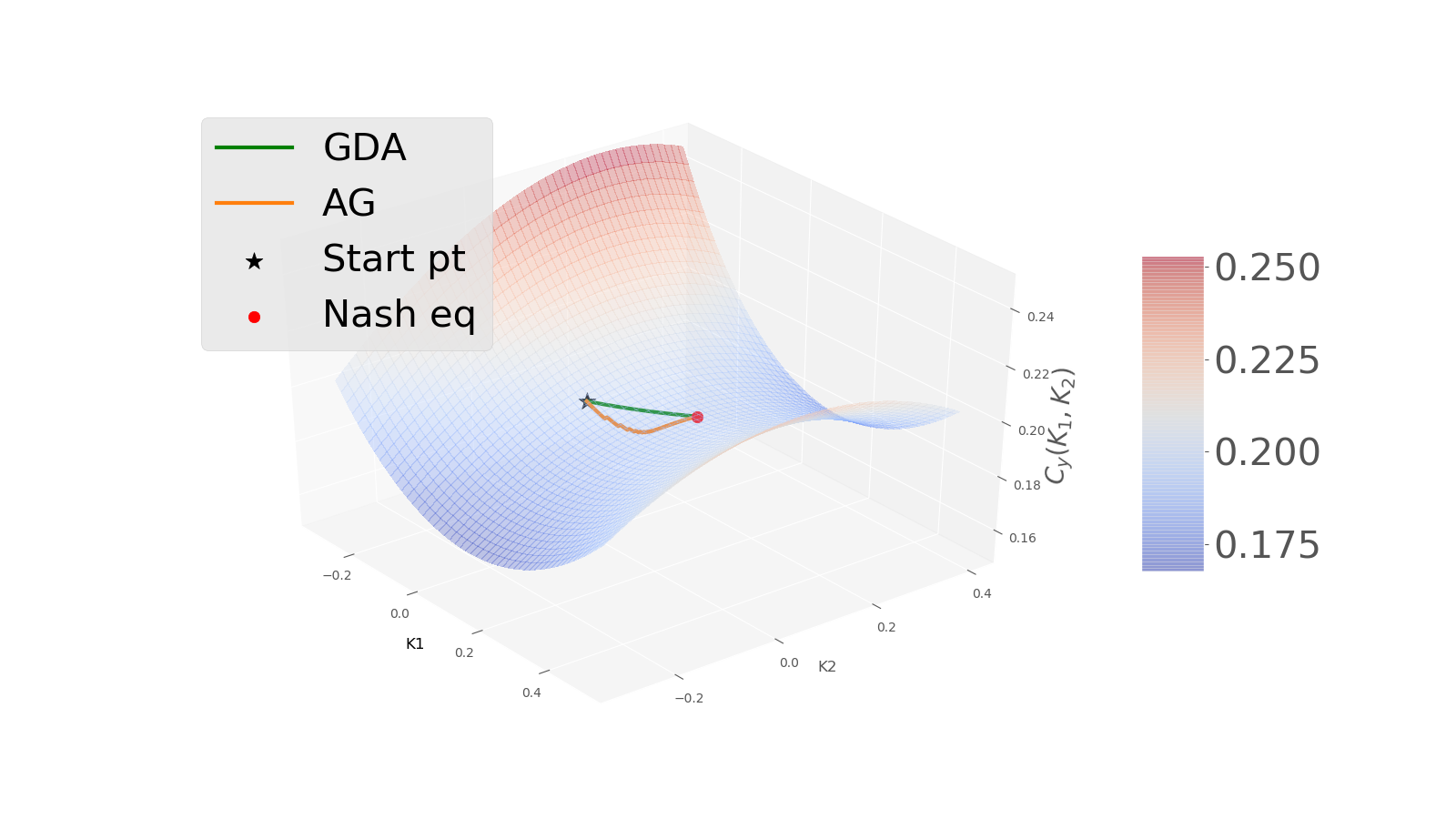
(a)  

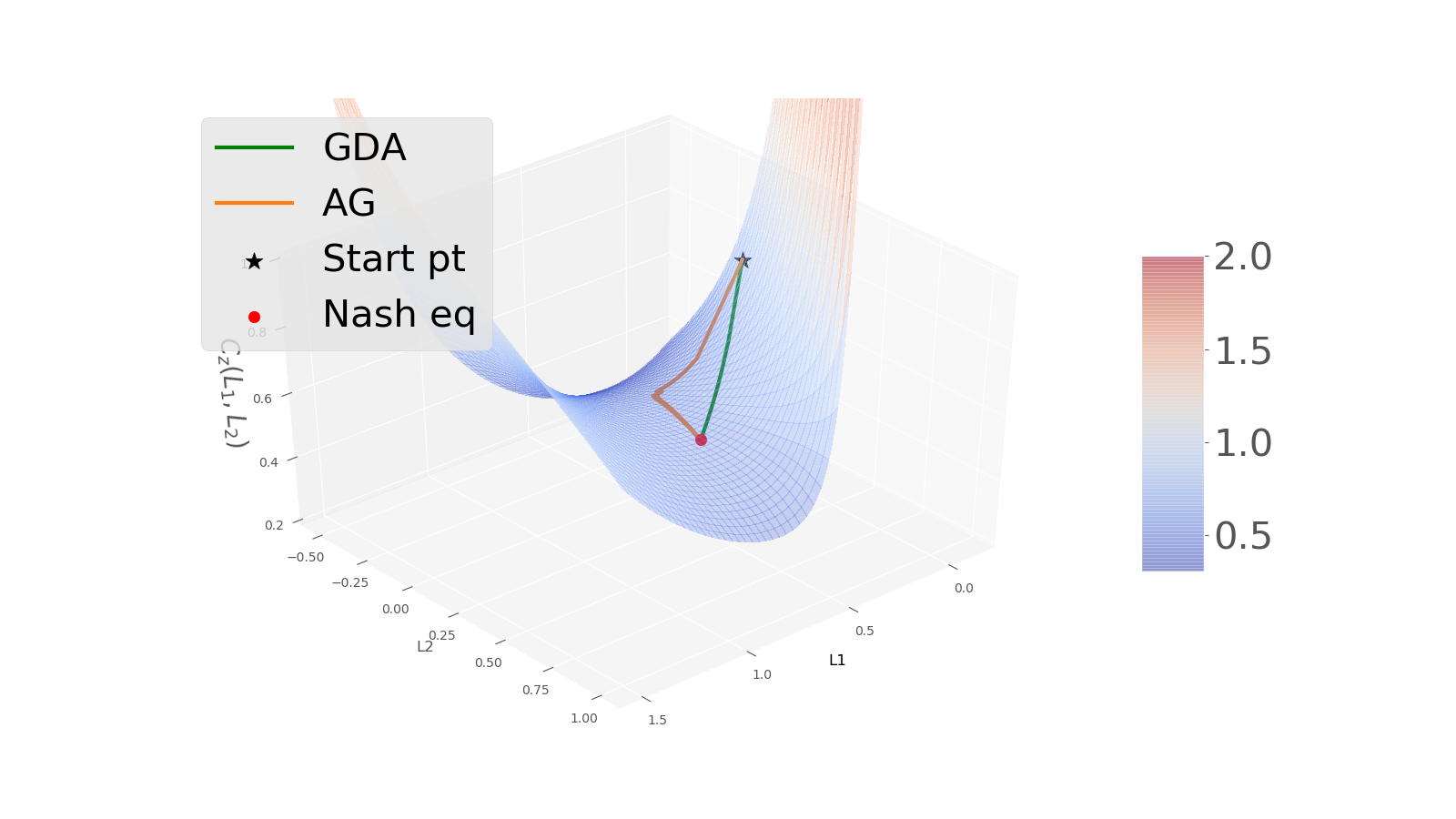
(b)  

Figure 1. Model-based policy optimization: Convergence of each part of the utility. (a) $C_{y}$ as a function of $(K_{1},K_{2})$. (b) $C_{z}$ as a function of $(L_{1},L_{2})$.

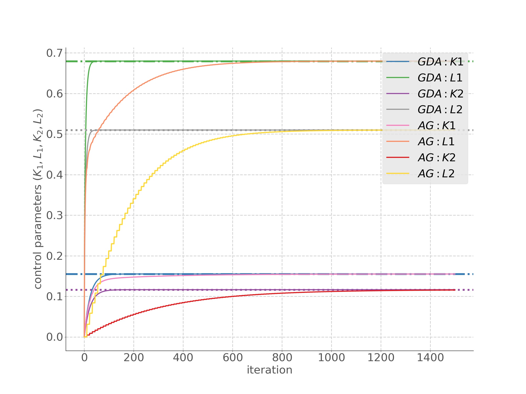
(a)  

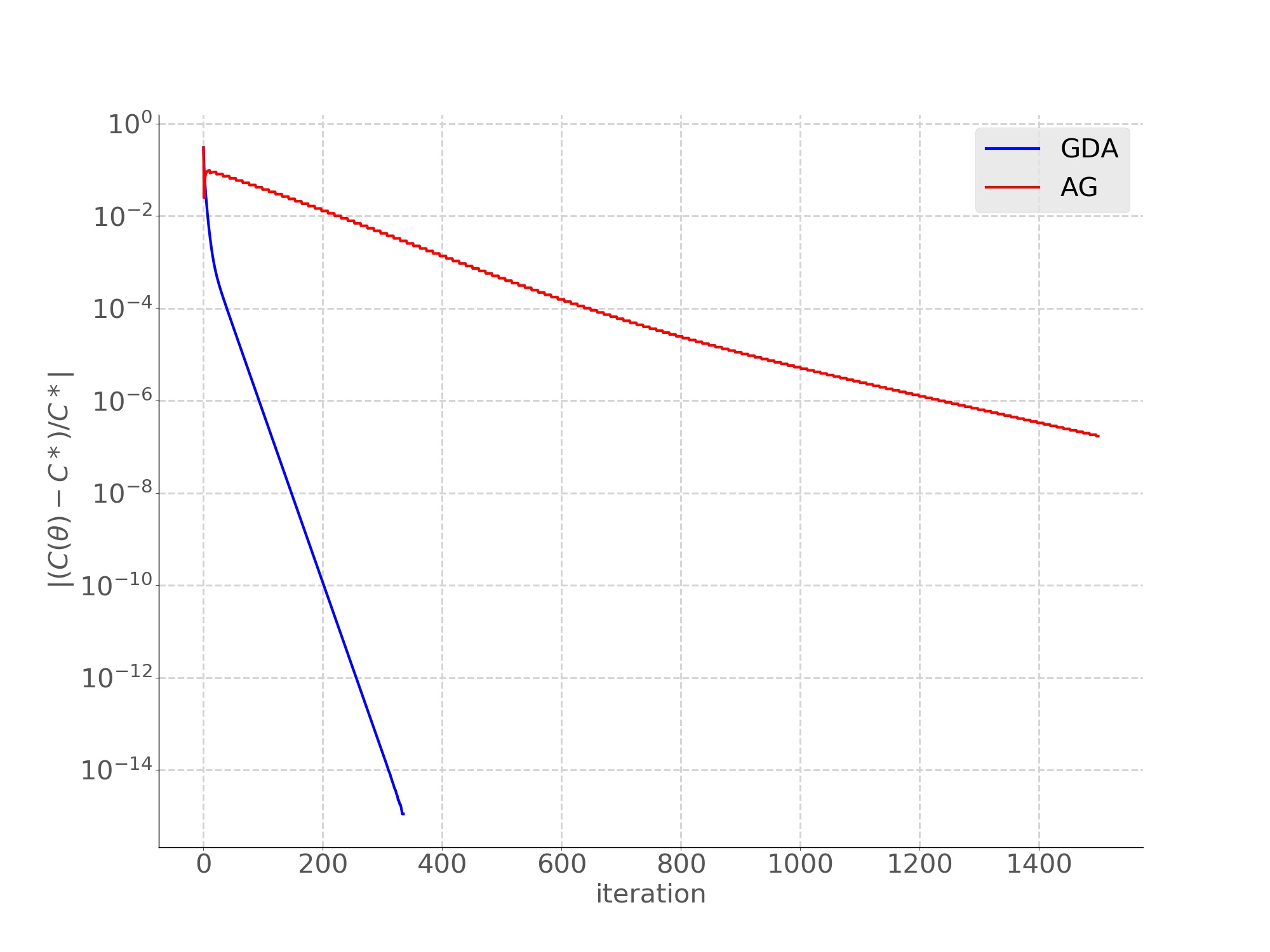
(b)  

Figure 2. Model-based policy optimization: Convergence of the control parameters in (a) and of the relative error on the utility in (b).

Sample-based results. The parameters used are given in Table 1 and were chosen based on the values in [28] as well as numerical experiments. The figures are obtained by averaging the results over 5 experiments, each based on a different realization of the randomness in the initial points, in the dynamics and in the gradient estimation.

Fig. 3 displays the trajectory of $(K_{1},K_{2})\mapsto C_{y}(K_{1},K_{2})$ and $(L_{1},L_{2})\mapsto C_{z}(L_{1},L_{2})$ generated by the iterations of AG and DGA methods. The convergence of the parameters $\theta=(K_{1},L_{1},K_{2},L_{2})$ is shown in Fig. 4(a). The evolution of the relative error on the utility is shown in Fig. 4(b).

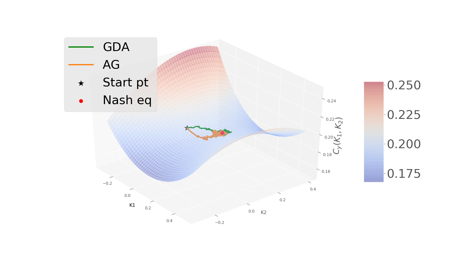
(a)  

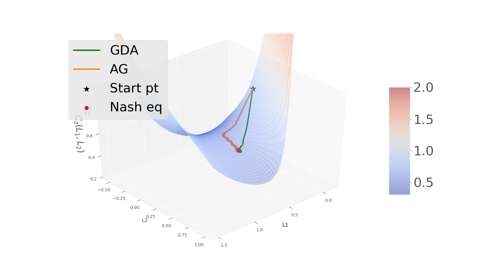
(b)  

Figure 3. Sample-based policy optimization: Convergence of each part of the utility. (a) $C_{y}$ as a function of $(K_{1},K_{2})$. (b) $C_{z}$ as a function of $(L_{1},L_{2})$.

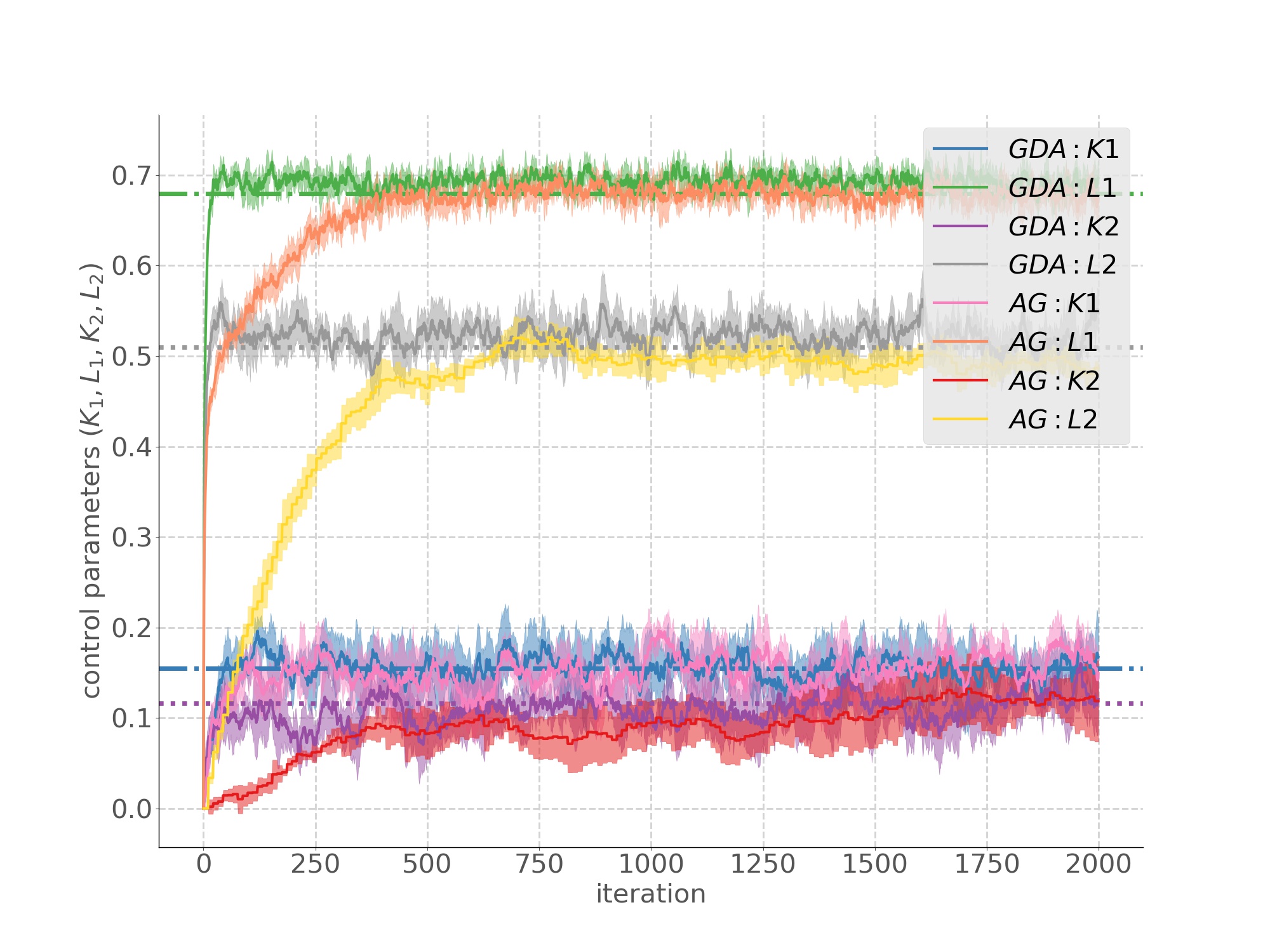
(a)  

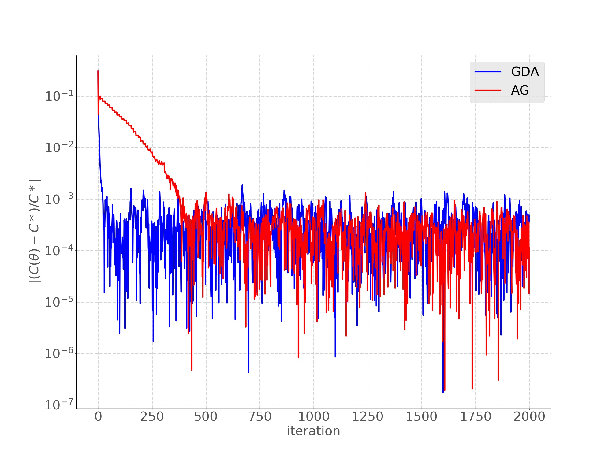
(b)  

Figure 4. Sample-based policy optimization: Convergence of the control parameters in (a) and of the relative error on the utility in (b).

Table 1. Simulation parameters

Model parameters $A$ $\overline{A}$ $B_{1}=\overline{B}_{1}$ $B_{2}=\overline{B}_{2}$ $Q$ $\overline{Q}$ $R_{1}=\overline{R}_{1}$ $R_{2}=\overline{R}_{2}$ $\gamma$ 0.4 0.4 0.4 0.3 0.4 0.4 0.4 0.4 0.9 Initial distribution and noise processes $\epsilon_{0}^{0}$ $\epsilon^{1}_{0}$ $\epsilon^{0}_{t}$ $\epsilon^{1}_{t}$ $\mathcal{U}([-1,1])$ $\mathcal{U}([-1,1])$ $\mathcal{N}(0,0.01)$ $\mathcal{N}(0,0.01)$ AG and DGA methods parameters $\mathcal{N}^{max}_{1}$ $\mathcal{N}^{max}_{2}$ $T$ $\eta_{1}$ $\eta_{2}$ $K_{1}^{0}$ $L_{1}^{0}$ $K_{2}^{0}$ $L_{2}^{0}$ 10 200 2000 0.1 0.1 0.0 0.0 0.0 0.0 Gradient estimation algorithm parameters $\mathcal{T}$ $M$ $\tau$ 50 10000 0.1

8. Conclusion

In this paper, we have studied zero-sum mean-field type games with linear quadratic model under infinite-horizon discounted utility function. We have identified the closed-form expression of the Nash equilibrium controls as linear combinations of the state and its mean. Moreover, we have proposed two policy optimization methods to learn the equilibrium. Numerical results have shown the convergence of the two methods in both model-based and sample-based settings. The question of convergence of the algorithms proposed here as well as model-free methods for non-LQ or general-sum MFTG will be studied in future works.

References

• [1] Yves Achdou, Fabio Camilli, and Italo Capuzzo-Dolcetta. Mean field games: numerical methods for the planning problem. SIAM Journal on Control and Optimization, 50(1):77–109, 2012.
• [2] Yves Achdou and Italo Capuzzo-Dolcetta. Mean field games: numerical methods. SIAM J. Numer. Anal., 48(3):1136–1162, 2010.
• [3] Yves Achdou and Jean-Michel Lasry. Mean field games for modeling crowd motion. In Contributions to partial differential equations and applications, pages 17–42. Springer, 2019.
• [4] Yves Achdou and Mathieu Laurière. On the system of partial differential equations arising in mean field type control. Discrete Contin. Dyn. Syst., 35(9):3879–3900, 2015.
• [5] Yves Achdou and Mathieu Laurière. Mean field type control with congestion (II): An augmented Lagrangian method. Appl. Math. Optim., 74(3):535–578, 2016.
• [6] Yves Achdou and Mathieu Laurière. Mean field games and applications: Numerical aspects. arXiv preprint arXiv:2003.04444, 2020.
• [7] Asma Al-Tamimi, Frank L Lewis, and Murad Abu-Khalaf. Model-free q-learning designs for linear discrete-time zero-sum games with application to h-infinity control. Automatica, 43(3):473–481, 2007.
• [8] Clémence Alasseur, Imen Ben Tahar, and Anis Matoussi. An extended mean field game for storage in smart grids. arXiv preprint arXiv:1710.08991, 2017.
• [9] Berkay Anahtarci, Can Deha Kariksiz, and Naci Saldi. Value iteration algorithm for mean-field games. arXiv preprint arXiv:1909.01758, 2019.
• [10] Julian Barreiro-Gomez, Tyrone E Duncan, and Hamidou Tembine. Discrete-time linear-quadratic mean-field-type repeated games: Perfect, incomplete, and imperfect information. Automatica, 112:108647, 2020.
• [11] Tamer Başar and Pierre Bernhard. H-infinity optimal control and related minimax design problems: a dynamic game approach. Springer Science & Business Media, 2008.
• [12] Dario Bauso. Game theory with engineering applications. SIAM, 2016.
• [13] Dario Bauso, Hamidou Tembine, and Tamer Başar. Robust mean field games with application to production of an exhaustible resource. IFAC Proceedings Volumes, 45(13):454–459, 2012.
• [14] Alain Bensoussan, Giuseppe Da Prato, Michel C Delfour, and Sanjoy K Mitter. Representation and control of infinite dimensional systems. Springer Science & Business Media, 2007.
• [15] Alain Bensoussan, Jens Frehse, and Sheung Chi Phillip Yam. Mean field games and mean field type control theory. Springer Briefs in Mathematics. Springer, New York, 2013.
• [16] Alain Bensoussan, Tao Huang, and Mathieu Laurière. Mean field control and mean field game models with several populations. arXiv preprint arXiv:1810.00783, 2018.
• [17] Luis M. Briceño Arias, Dante Kalise, Ziad Kobeissi, Mathieu Laurière, Álvaro Mateos González, and Francisco J. Silva. On the implementation of a primal-dual algorithm for second order time-dependent mean field games with local couplings. ESAIM: ProcS, 65:330–348, 2019.
• [18] Luis M. Briceño Arias, Dante Kalise, and Francisco J. Silva. Proximal methods for stationary mean field games with local couplings. SIAM J. Control Optim., 56(2):801–836, 2018.
• [19] Haoyang Cao, Xin Guo, and Mathieu Laurière. Connecting gans and mfgs. arXiv preprint arXiv:2002.04112, 2020.
• [20] Pierre Cardaliaguet. Notes on mean field games, 2013.
• [21] Pierre Cardaliaguet and Charles-Albert Lehalle. Mean field game of controls and an application to trade crowding. Mathematics and Financial Economics, 12(3):335–363, 2018.
• [22] E. Carlini and F. J. Silva. A fully discrete semi-Lagrangian scheme for a first order mean field game problem. SIAM J. Numer. Anal., 52(1):45–67, 2014.
• [23] René Carmona and François Delarue. Probabilistic Theory of Mean Field Games with Applications I-II. Springer, 2018.
• [24] René Carmona, Jean-Pierre Fouque, and Li-Hsien Sun. Mean field games and systemic risk. Commun. Math. Sci., 13(4):911–933, 2015.
• [25] René Carmona, Kenza Hamidouche, Mathieu Laurière, and Zongjun Tan. Policy Optimization for Linear-Quadratic Zero-Sum Mean-Field Type Games. Accepted to CDC’2020., 2020.
• [26] René Carmona and Mathieu Laurière. Convergence analysis of machine learning algorithms for the numerical solution of mean field control and games: I - the ergodic case, 2019.
• [27] René Carmona and Mathieu Laurière. Convergence analysis of machine learning algorithms for the numerical solution of mean field control and games: II - the finite horizon case. arXiv preprint arXiv:1908.01613, 2019.
• [28] René Carmona, Mathieu Laurière, and Zongjun Tan. Linear-quadratic mean-field reinforcement learning: convergence of policy gradient methods. arXiv preprint arXiv:1910.04295, 2019.
• [29] René Carmona, Mathieu Laurière, and Zongjun Tan. Model-free mean-field reinforcement learning: mean-field mdp and mean-field q-learning. arXiv preprint arXiv:1910.12802, 2019.
• [30] Andrea Cosso and Huyên Pham. Zero-sum stochastic differential games of generalized mckean–vlasov type. Journal de Mathématiques Pures et Appliquées, 129:180–212, 2019.
• [31] Boualem Djehiche and Said Hamadène. Optimal control and zero-sum stochastic differential game problems of mean-field type. Appl. Math. Optim., 81(3):933–960, 2020.
• [32] Boualem Djehiche, Alain Tcheukam, and Hamidou Tembine. Mean-field-type games in engineering. arXiv preprint arXiv:1605.03281, 2016.
• [33] Carles Domingo-Enrich, Samy Jelassi, Arthur Mensch, Grant Rotskoff, and Joan Bruna. A mean-field analysis of two-player zero-sum games. arXiv preprint arXiv:2002.06277, 2020.
• [34] Romuald Élie, Tomoyuki Ichiba, and Mathieu Laurière. Large banking systems with default and recovery: A mean field game model. arXiv preprint arXiv:2001.10206, 2020.
• [35] Romuald Elie, Julien Perolat, Mathieu Laurière, Matthieu Geist, and Olivier Pietquin. On the convergence of model free learning in mean field games. In AAAI Conference one Artificial Intelligence (AAAI 2020).
• [36] Maryam Fazel, Rong Ge, Sham M Kakade, and Mehran Mesbahi. Global convergence of policy gradient methods for the linear quadratic regulator. arXiv preprint arXiv:1801.05039, 2018.
• [37] Haotian Gu, Xin Guo, Xiaoli Wei, and Renyuan Xu. Q-learning for mean-field controls. arXiv preprint arXiv:2002.04131, 2020.
• [38] Xin Guo, Anran Hu, Renyuan Xu, and Junzi Zhang. Learning mean-field games. In Advances in Neural Information Processing Systems, pages 4967–4977, 2019.
• [39] Minyi Huang, Roland P. Malhamé, and Peter E. Caines. Large population stochastic dynamic games: closed-loop McKean-Vlasov systems and the Nash certainty equivalence principle. Commun. Inf. Syst., 6(3):221–251, 2006.
• [40] Hyesung Kim, Jihong Park, Mehdi Bennis, Seong-Lyun Kim, and Mérouane Debbah. Mean-field game theoretic edge caching in ultra-dense networks. IEEE Transactions on Vehicular Technology, 2019.
• [41] Vladimír Kučera. The discrete riccati equation of optimal control. Kybernetika, 8(5):430–447, 1972.
• [42] Jean-Michel Lasry and Pierre-Louis Lions. Mean field games. Japanese journal of mathematics, 2(1):229–260, 2007.
• [43] Zhiyu Liu, Bo Wu, and Hai Lin. A mean field game approach to swarming robots control. In 2018 Annual American Control Conference (ACC), pages 4293–4298, 2018.
• [44] Tzon-Tzer Lu and Sheng-Hua Shiou. Inverses of 2$\times$ 2 block matrices. Computers & Mathematics with Applications, 43(1-2):119–129, 2002.
• [45] François Mériaux, Vineeth Varma, and Samson Lasaulce. Mean field energy games in wireless networks. In 2012 conference record of the forty sixth Asilomar conference on signals, systems and computers (ASILOMAR), pages 671–675, 2012.
• [46] ACM Ran and R Vreugdenhil. Existence and comparison theorems for algebraic riccati equations for continuous-and discrete-time systems. Linear Algebra and its applications, 99:63–83, 1988.
• [47] Dian Shi, Hao Gao, Li Wang, Miao Pan, Zhu Han, and H Vincent Poor. Mean field game guided deep reinforcement learning for task placement in cooperative multi-access edge computing. IEEE Internet of Things Journal, 2020.
• [48] Jingrui Sun, Jiongmin Yong, and Shuguang Zhang. Linear quadratic stochastic two-person zero-sum differential games in an infinite horizon. ESAIM: Control, Optimisation and Calculus of Variations, 22(3):743–769, 2016.
• [49] John Von Neumann and Oskar Morgenstern. Theory of games and economic behavior (commemorative edition). Princeton university press, 2007.
• [50] Ruimin Xu. Zero-sum stochastic differential games of mean-field type and bsdes. In Proceedings of the 31st Chinese Control Conference, pages 1651–1654, 2012.
• [51] Kaiqing Zhang, Zhuoran Yang, and Tamer Basar. Policy optimization provably converges to nash equilibria in zero-sum linear quadratic games. In Advances in Neural Information Processing Systems, pages 11598–11610, 2019.